1

Simplified Swarm Optimisation for the Hyperparameters of a

Convolutional Neural Network

Wei-Chang Yeh1, Yi-Ping Lin1, Yun-Chia Liang2, Chyh-Ming Lai3, and Xiao-Zhi Gao4 1 Department of Industrial Engineering and Engineering Management, National Tsing Hua

University, Taiwan. 2 Industrial Engineering and Management, Yuan Ze University, Taiwan. 3 Management College, National Defense University, Taiwan. 4 School of Computing, University of Eastern Finland, Kuopio, Finland

Convolutional neural networks (CNNs) are widely used in image recognition. Numerous CNN

models, such as LeNet, AlexNet, VGG, ResNet, and GoogLeNet, have been proposed by

increasing the number of layers, to improve the performance of CNNs. However, performance

deteriorates beyond a certain number of layers. Hence, hyperparameter optimisation is a more

efficient way to improve CNNs. To validate this concept, a new algorithm based on simplified

swarm optimisation is proposed to optimise the hyperparameters of the simplest CNN model,

which is LeNet. The results of experiments conducted on the MNIST, Fashion MNIST, and

Cifar10 datasets showed that the accuracy of the proposed algorithm is higher than the original

LeNet model and PSO-LeNet and that it has a high potential to be extended to more complicated

models, such as AlexNet.

Keywords: Machine Learning; Image Recognition; Convolutional Neural Networks; Simplified

Swarm Optimization; Hyper-parameter Optimization.

Corresponding author: W.C. Yeh; email: yeh@ieee.org

1. INTRODUCTION

Deep learning, a special machine learning method based on an artificial neural network

(ANN), has recently gained popularity. Deep learning makes a machine intelligent such that a

computer can simulate the functions of the human brain to observe, analyse, learn human

behaviour, and make decisions.

2

Among deep learning applications, including image recognition [1], artistic creation [2],

semantic understanding [3], and poetry creation [4], image recognition has become the most

popular research field in recent years. In addition, image recognition is an important task that

can be applied to transportation, home, manufacturing, and medical applications, such as

autonomous driving [7], healthcare [8], product defect detection [9], and medical imaging [10,

11], making people's lives more convenient.

Convolutional neural networks (CNNs) are the most intensively researched [12] models

for image recognition because they are more accurate than human judgement [13]. With the

combination of three layers (that is, the convolution, pooling, and fully connected layers) and

one function, CNNs have considerable flexibility to allow users to make modifications

according to their needs.

The history of CNNs can be traced back to 1962 [14]; however, the model that is closest

to the present definition of a CNN is the LeNet proposed by Yann LeCun in 1989, and it has

been revised repeatedly since then [15]. After the proposal of AlexNet [1] in 2012, there have

been significant advancements in CNNs. Many CNN models, such as VGG, ResNet, and

GoogLeNet, have been developed successively [17-20].

Increasing the number of layers leads to less accurate results [21]. Hence, numerous

studies have investigated methods to improve CNN performance without changing the

architecture. Hyperparameters include the size of kernels, number of kernels, length of strides,

and pooling size, which directly affect the performance and training speed of CNNs. Moreover,

the impact of hyperparameters increases as the complexity of the network increases. Hence, the

most popular method of improving CNN performance is to optimise the hyperparameters [22,

23].

CNN hyperparameter optimisation is an integer programming problem. In the past, many

studies used manual designs for hyperparameters; that is, scholars or experts must adjust the

3

hyperparameters based on experience and expertise, which is not only unfounded but also time

consuming during testing. Several heuristic approaches, such as a grid search, randomised

search [27], Bayesian optimisation, and gradient-based optimisation, have been developed for

hyperparameter optimisation. The drawback of the above methods is that they are less efficient

in a high-dimensional space because the number of evaluations increases exponentially as the

number of hyperparameters increases [28-30].

Hence, artificial intelligence techniques, including the genetic algorithm [34-37], particle

swarm algorithm (PSO) [38-40], and artificial bee colony algorithm [41], have been proposed

for this problem. However, most of these methods change the CNN structure or combine

different algorithms to optimise the performance and are complicated and difficult for users to

understand. Thus, there is a need for a simple algorithm that does not change the CNN structure

for the hyperparameters.

The purpose of this study is to apply the simplified swarm optimisation (SSO) algorithm

proposed by Yeh to tune the CNN hyperparameters [6]. The SSO is not only simple and easy

to understand but also efficient. Many studies have demonstrated the excellent ability of SSO

in optimisation problems [42-46]; however, no research has applied SSOs to the

hyperparameter optimisation problem. Therefore, in this study, a new algorithm called the SSO-

LeNet is proposed to apply SSO to the original LeNet architecture without changing the layers

and validate it with different datasets for automated hyperparameter optimisation.

The remainder of this paper is organised as follows. Section 2 provides an overview of

CNNs, LeNet, and SSO, which are the basis of the proposed algorithm. Section 3 describes the

major parts of the proposed SSO-LeNet, including the special solution structure, fitness

function, sequential dynamic variable range (SDVR), and small-sample design matrix. Section

4 provides the pseudocode and flowchart for further details. Section 5 describes three

experiments: Ex1, Ex2, and Ex3, on three benchmark datasets, including NMIST, Fashion-

4

MNIST, and CIFAR10, to demonstrate ways to use the proposed SDVR and the small-sample

design matrix in Ex1, and then compares the proposed SSO-LeNet to the traditional LeNet [49]

and PSO-LeNet [39] in Ex2 and Ex3, respectively. Finally, Section 6 concludes the study and

provides possible future work.

2. OVERVIEW OF ANN, CNN, LENET, AND SSO

ANNs are the basis of CNNs and LeNet [49] is the simplest CNN that we propose an

SSO-based algorithm to optimise its hyperparameters. Hence, ANNs, CNNs, LeNets, and SSOs

are reviewed in this section before introducing the proposed SSO-LeNet.

2.1 Artificial Neural Network

An ANN, also known as a multi-layer perceptron, is a special network model comprising

many nodes and arcs, as shown in Fig. 1. These nodes mimic human nerve cells, called neurons,

and transmit information to the next layer by connecting neurons in different layers. Every

neuron in each layer is connected to all the neurons in the next layer; however, neurons in the

same layer are not connected.

As the depth of a neural network increases, a deeper ANN with more hidden layers, called

a deep neural network, can be used to solve problems that are more complex [5, 6].

Figure 1. ANN Structure

2.2 Convolutional Neural Network

A CNN is developed from an ANN, as shown in Fig. 2; therefore, it also has an input

layer, hidden layers, and an output layer. To extract features and classify images, four main

5

operations are used to build a CNN model. These operations are described in detail in Sections

2.2.1–2.2.4.

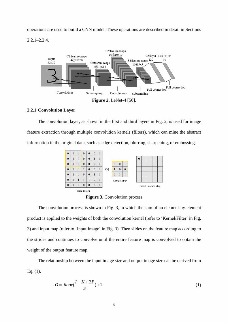
Figure 2. LeNet-4 [50].

2.2.1 Convolution Layer

The convolution layer, as shown in the first and third layers in Fig. 2, is used for image

feature extraction through multiple convolution kernels (filters), which can mine the abstract

information in the original data, such as edge detection, blurring, sharpening, or embossing.

Figure 3. Convolution process

The convolution process is shown in Fig. 3, in which the sum of an element-by-element

product is applied to the weights of both the convolution kernel (refer to ‘Kernel/Filter’ in Fig.

3) and input map (refer to ‘Input Image’ in Fig. 3). Then slides on the feature map according to

the strides and continues to convolve until the entire feature map is convolved to obtain the

weight of the output feature map.

The relationship between the input image size and output image size can be derived from

Eq. (1).

2( ) 1I K P

O floorS

− += + (1)

6

Here,

⚫ O and I denote the size of the output and input images, respectively;

⚫ K represents the size of the kernel;

⚫ P indicates the number of zero-padding that fills the boundary of the feature

image with zero weight; and

⚫ S is the symbol for the size of the stride, which is the number of pixel shifts

over the input image.

For example, in Fig. 2, let the size of the input image be 5 5, the size of the convolution

kernel be 3 3, the stride be 1, and the zero-padding be used. The size of the output feature

after convolution is 5 5.

2.2.2 Pooling Layer

Generally, the convolution layer outputs a feature map to the pooling layers, as depicted

in the second and fourth layers of Fig. 2, which is also known as the subsampling layer. Pooling

layers avoid overfitting by pooling the convolved feature map, decreasing the dimensionality

of the feature map, reducing sampling, and retaining important features.

Figure 4. Pooling process

There are two common pooling methods: average pooling and maximum pooling, which

operate similarly to convolution. The size and strides of the pooling window must first be

determined. The pooling process is shown in Fig. 4.

7

Pooling considers the average or maximum value of a local block; slight distortions in the

input image do not affect the output image, and the output can be obtained in almost the same

proportion as the input image.

In addition, the output size of the feature map after the pooling layer can be obtained

using Eq. (1).

2.2.3 Fully Connected Layer

As demonstrated in Fig. 2, the first half of the CNN comprises multiple convolution layers

(i.e., the first and the third layers) and pooling layers (i.e., the second and fourth layers)

alternately for extracting and learning features. The second half is created after flattening

(which is the input layer of the fully connected layer; refer to the first ‘Full connection’ in Fig.

2).

The second half comprises a fully connected layer and an output layer for image

classification. The fully connected layer is similar to the traditional ANN in which the neurons

in each layer are connected to all the neurons in the next layer, and the final output layer outputs

the final image classification based on the classifier. A common classifier is the softmax

function, which normalises the feature map vectors to values between [0, 1] for each category.

2.2.4 Activation Function

The activation functions transfer linear functions into nonlinear operations so that the

ANN can solve more complex problems, such as a nonlinear classification problem.

Common activation functions include the sigmoid, tanh, and rectified linear units (ReLU)

functions, as shown in Fig. 5. Among these functions, the most popular is the ReLU function,

which has been proven to have the same or better performance than the sigmoid and tanh

functions [47, 48]. Moreover, it not only avoids the vanishing gradient problem but also

improves the complexity of time and space with a lower computational cost.

8

Figure 5. Common activation functions

2.3 LeNet

Since Yann LeCun proposed LeNet-1 in 1989, he continued revising it and finally

proposed LeNet-5 to solve the problem of handwriting recognition in 1998; he also proposed

the MNIST dataset comprising handwritten digits, which was successfully applied to the U.S.

postal handwriting code recognition [49]. The LeNet-4 model is shown in Fig. 2 [50].

Table 1. LeNet-4 structure and hyperparameters

Layers Hyperparameters

Convolution Layer (C1) Number of kernels: 4

Size of kernels: 55

Strides: 11

Pooling Layer (P2) Size of pooling: 22

Strides: 22

Convolution Layer (C3) Number of kernels: 16

Size of kernels: 55

Strides: 11

Pooling Layer (P4) Size of pooling: 55

Strides: 11

Convolution Layer (C5) Number of kernels: 120

Size of kernels: 55

Strides: 11

Fully Connected Layer (FC6) 120 units

Output Layer 10 classifications

Sigmoid Tanh ReLU

𝑓ሺ𝑥ሻ =1

1 + 𝑒−𝑥 𝑡𝑎𝑛ℎሺ𝑥ሻ =

2

1 + 𝑒−2𝑥− 1 𝑓ሺ𝑥ሻ = ൜

0 𝑓𝑜𝑟 𝑥 ≤ 0𝑥 𝑓𝑜𝑟 𝑥 > 0

9

First, a handwritten digital image is input, which is then convolved three times via C1,

C3, and C5 and pooled twice (P2 and P4), followed by a fully connected layer (FC6). Finally,

the output layer outputs the digital category from 0 to 9. The LeNet-4 structure and

hyperparameters are presented in Table 1.

2.4 Simplified Swarm Optimisation

The SSO algorithm was proposed by Yeh in 2009 [51], and it is known to be the simplest

machine learning method. SSOs have been widely applied in many fields, such as redundancy

allocation problems [38], data mining [42], health care management [46], and disassembly

sequencing problems [43] [52].

Let Xi = (xi,1, xi,2, …, xi,Nvar) denote the solution i and xi,j be its jth variable, where Nvar is

the number of variables. Assign pBest Pi = (pi,1, pi,2, …, pi,Nvar), which is the personnel leader,

to be the best solution among its own evolutionary history, and gBest G = PgBest = (G1, G2, …,

GNvar), which is the global leader, to be the best solution among all others.

SSO is a population-based stochastic optimisation technique, a swarm intelligence

method, and an evolutionary computing technique. The swarm intelligence algorithm follows

the leaders, that is, G = (G1, G2, …, GNvar) and Pi = (pi,1, pi,2, …, pi,Nvar), to update the solutions;

the most important operation in evolutionary computing is the update mechanism, which

iterates continuously to obtain a solution that is close to the optimal solution.

The updating mechanism of SSO is the stepwise function listed in Eq. (2):

[0,1]

, [0,1]

,

[0,1],

[0,1]

if ρ [0, )

if ρ [ , ) if ρ [ , )

if ρ [ ,1]

j g g

i j g g p p

i j

g p g p w wi j

g p w

g c C

p c c c Cx

c c c c c Cx

c c cx

=

+ ==

+ + + = + +

(2)

The update of each xi depends on one random variable [0,1] generated uniformly between

0 and 1. cg = Cg cp = (Cp − Cg) cw = (Cw − Cp) cr = (1 − Cw) are the probabilities that the

10

newly updated xi,j is equal to gj, pi,j, xi,j (no change) and a random feasible value x, respectively.

Note that cg + cp + cw + cr = 1.

This four-term stepwise function update mechanism is efficient in balancing the

exploration and exploitation abilities.

3. MAJOR COMPONENTS OF THE SSO-LeNet

This section introduces the major components of the proposed SSO-LeNet, including the

solution structure to encode the CNN network structure, the fitness for SSO-LeNet to learn to

improve itself, SDVR to adjust feasible region self-adaptively, and small-sample design matrix

to tune the SSO parameters Cg, Cp, and Cw systematically and efficiently. The last two

components are novel to SSO-LeNet.

3.1 Solution Structure

The CNN structure consists of hyperparameters including the number and size of the

kernels in each convolution layer, the size of the stride, and the size of the kernels in the pooling

layer. Each solution in the proposed SSO-LeNet is the same as the hyperparameter settings of

the CNN. Hence, the solution encoding is based on the original structure of LeNet without the

need to add or delete a layer.

As shown in Figs. 2 and 6, there are 16 variables in LeNet. Thus, each solution, for

example, X = (x1, x2, …, x16), represents the 16 hyperparameters of LeNet. Their meanings and

their value ranges are provided in Table 2.

Figure 6. Hyperparameters encoding of the LeNet structure

11

Table 2. Meanings and range of values of hyperparameters

Variable Symbol Hyperparameter Range

x1 N1 The number of kernels of the first

convolution layer.

[16, 24, 32, 40, 48, 52, 64]

x2 K1,x The x-axis size, i.e., the number of

columns of kernels of the first

convolution layer.

[2 – min{11, Inputx}]

x3 K1,y The size of the y-axis, i.e., the

number of rows of kernels of the

first convolution layer.

[2 – min{11, Inputy}]

x4 S1,x The stride of the x-axis of the first

convolution layer.

[1 − 4]

x5 S1,y The stride of the y-axis of the first

convolution layer.

[1 − 4]

x6 P1,x The x-axis size of the first pooling

layer.

[1 − 𝑂1𝑥]

x7 P1,y The size of the y-axis of the first

pooling layer.

[1 – 𝑂1𝑦

]

x8 N2 The number of kernels of the second

convolution layer.

[16, 24, 32, 40, 48, 52, 64]

x9 K2,x The x-axis size of kernels of the

second convolution layer.

[1 – 𝑂2𝑥]

x10 K2,y The size of the y-axis of kernels of

the second convolution layer.

[1 – 𝑂2𝑦

]

x11 S2,x The stride of the x-axis of the

second convolution layer.

[1 – min(4, 𝑂2𝑥ሻ]

x12 S2,y The stride of the y-axis of the

second convolution layer.

[1 – min(4, 𝑂2𝑦ሻ]

x13 P2,x The x-axis size of the second

pooling layer.

[1 – 𝑂3𝑥]

x14 P2,y The size of the y-axis of the second

pooling layer.

[1 – 𝑂3𝑦

]

x15 𝑈 The units of a fully connected layer. [50 – 150]

x16 b The size of a training batch. [10 – 30]

In Table 2, Inputx and Inputy are the sizes of the x- and y-axes of the input images,

respectively. The notation Ni represents the number of kernels in the ith convolution layer.

The symbols K, P, and S denote the kernel, pooling, and stride, respectively. The first

subscript, say i, implies that it belongs to the ith convolution layer or pooling layer depending

12

on the capital letter. The second subscript, j, indicates that it is related to the x-axis or y-axis.

For example, Ki,x denote the x-axis sizes of the kernels in the ith convolution layer.

3.2 Fitness Function

According to Section 3.1, each solution represents a hyperparameter configuration that is

a CNN structure. These hyperparameters are trained by executing LeNet and learn to improve

from the fitness function, which denotes the accuracy of the testing data for each solution and

is formulated as follows:

Ftest = 1

testN

i

i test

a

N=

(3)

where

1 if the th sample predicted correctly

0 otherwisei

ia

=

(4)

Ntest represents the size of testing data.

3.3 Sequential Dynamic Variable Range

In a traditional SSO, each solution is initialised feasibly and randomly. Owing to the

operation of the CNN, the feature map becomes increasingly smaller. Hence, to ensure that the

output size of the previous layer does not equal the input size of the current layer, a novel

mechanism called the SDVR is proposed.

In each solution of the proposed algorithm, variables are updated one by one, as in most

SSOs. However, unlike most SSOs, the feasible range of the next variable, xi, is dependent on

the value of the current variable, xi-1, in the proposed algorithm.

For example, if the size of the input image is 28 28, and we have generated the first five

variables, which are 52-8-11-1-1, then the sixth variable representing the x-axis size of the first

pooling layer, as shown in Table 2, has to be larger than 1 and smaller than the output size of

13

the last convolution layer 𝑂1𝑥. Thus, we know that the sixth variable can only be randomly

generated within [1, 21] based on Eq. (1).

3.4 Small-sample Design Matrix

Not only do the hyperparameters in LeNet need to be tuned but also the SSO parameters

and variables in Eq. (2). To achieve the above two goals simultaneously, in this study, we

applied three different parameter settings, as listed in Table 3.

Table 3. Design matrix.

Row Cg Cp Cw

1 0.4 0.7 0.9

2 0.5 0.5 0.8

3 0.5 0.7 0.7

In row 1, three parameters are under normal settings such that Cg Cp Cw and cg = 0.4,

cp = 0.3, cw = 0.2, and cr = 0.1, without removing any item from Eq. (2). Note that cg and cr are

smaller than those in the other settings, for example, cg = 0.5 and cr = 0.2 in row 2. Row 2 sets

Cg = Cp = 0.5, with a medium probability of cr = 0.2. The goal of row 2 is to test whether the

result is better if the role of pBest and a medium value of cr are removed. Row 3 assigns Cp =

Cw = 0.7 to remove the third item from Eq. (2) with a larger value of cr = 0.3, which has a higher

chance of escaping local traps but a weak convergence to the optimum.

Deep learning requires a certain amount of time to train big data. In addition, SSO requires

at least 30 runs and a certain number of generations and solutions to update the solutions for a

better result. In the proposed SSO-LeNet, one solution update is to execute LeNet based on the

structure encoded in the solution. For example, if Nrun = 10, Ngen = 20, and Nsol = 4, we need to

run LeNet for 800 times (10 20 4).

Hence, to reduce the training time and to find a better set of parameters, in the small

sample, we only used five runs to train different SSO parameter settings and evaluated the

accuracy to obtain the best configuration for this model. Specifically, to evaluate the

14

performance of these three rows with a more robust result, a small sampling test and one-way

ANOVA test were performed. Each row corresponded to an SSO with the setting shown in the

design matrix. Each SSO was executed in five runs, that is, a small sampling test was conducted

on three benchmark datasets: MNIST, Fashion-MNIST, and Cifar10.

The details of the small sampling test and one-way ANOVA test are provided in Section

5.2.

4. PROPOSED SSO-LENET

This section describes the detailed procedure of SSO-LeNet and illustrates the process

through pseudocode and a flowchart.

4.1 Update Mechanism of the SSO-LeNet

In machine learning, parameters are the most important elements in both the update and

selection procedures. The tuning of the parameters significantly affects the results. In SSOs,

there are two possible methods to improve the quality of a solution: parameter-tuning and item-

tuning. The former changes the value of the parameter, while the latter adds or removes items,

such as Eqs. (5) and (6) removing the second and third items from Eq. (2), respectively. In this

study, we used both methods to improve the quality of the solution.

[0,1]

, , [0,1]

[0,1]

if ρ [0, )

if ρ [ , )

if ρ [ ,1]

jg g

i j i j g p g p w w

g p w

g c C

x x c c c c c C

c c cx

=

= + + + = + +

(5)

[0,1]

, , [0,1]

[0,1]

if ρ [0, )

if ρ [ , )

if ρ [ ,1]

j g g

i j i j g g p p

g p w

g c C

x p c c c C

c c cx

=

= + = + +

. (6)

15

4.2 Stopping Criteria of SSO-LeNet

All algorithms have different stopping criteria according to different conditions. As

mentioned in Section 3.4, a CNN always takes a long time to execute. To stop the execution of

the algorithm earlier, is the generation in which the accuracy obtained from the proposed

algorithm starts better than that of LeNet is considered as the stopping criterion.

4.3 Pseudocode and Flowchart

Let Ngen, Nsol, and Nvar be the number of generations, solutions, and variables, respectively.

We assume that Z is the solution obtained from LeNet. The pseudocode of the proposed SSO-

LeNet is as follows.

STEP 0. Generate a solution of hype-parameters Z and calculate its fitness F(Z) using LeNet.

STEP 1. Initialise solutions Pi = Xi, calculate F(Pi) = F(Xi) for i = 1, 2, …, Nsol, find G =

F(PgBest), and let t = i = 1.

STEP 2. Update Xi based on the best parameter setting obtained using the small sampling

discussed in Section 3.4 and calculate F(Xi).

STEP 3. If F(Xi) is better than F(Pi), then Pi = Xi. Otherwise, return to STEP 5.

STEP 4. If F(Xi) is better than F(G), let G = Xi.

STEP 5. If i < Nsol, then i = i + 1 and return to STEP 2.

STEP 6a. If F(G) is better than F(Z), then stop.

STEP 6. If t < Ngen, then t = t + 1, i = 1, and return to STEP 2. Otherwise, stop.

Note that STEP 6a is an optional step and an early stopping criterion. When we implement

STEP 6a, the algorithm ends earlier. A flowchart of the proposed algorithm is shown in Fig. 7.

16

Figure 7. The flowchart of the proposed algorithm.

Start

Run LeNet once to have Z and F(Z)

Initialize Pi = Xi randomly, calculate

F(Xi), and find G for all i

Let t = 1 and i = 1.

Update Xi and calculate F(Xi).

F(Pi) < F(Xi)?

Let Pi = Xi and F(Pi) = F(Xi).

Let G = Xi and F(G) = F(Xi).

F(Gi) < F(Xi)?

Let i = i + 1.

F(Gi) < F(Z)?

Let t = t + 1 and i = 1

Halt

i < Nsol

?

t < Ngen

?

Yes

No

Yes

Yes

Yes

Yes

No

No

No

No

17

5. EXPERIMENTS

Three experiments, Ex1, Ex2, and Ex3, were conducted on three benchmark datasets:

MNIST, Fashion-MNIST, and Cifar10. Ex1 mainly tuned the parameters of the SSO using the

small-sample design matrix listed in Table 4. Based on the best SSO parameters selected in Ex1,

Ex2 and Ex3 were conducted to demonstrate the performance of the proposed SSO-LeNet by

comparing it to the traditional LeNet [49] and PSO-LeNet [39], respectively.

5.1 Three Datasets and Experiment Environments

Three datasets, namely MNIST, Fashion-MNIST, and Cifar10 [49], were used in the

experiments, and they are summarised as follows.

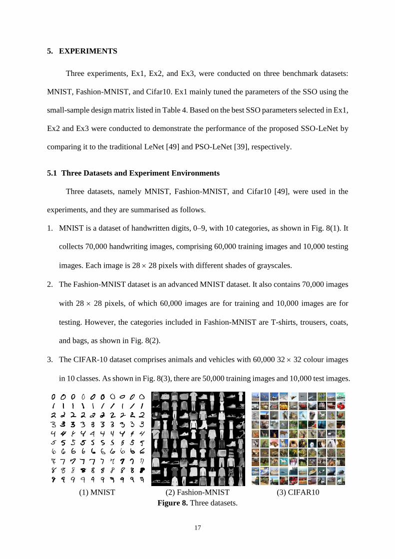
1. MNIST is a dataset of handwritten digits, 0–9, with 10 categories, as shown in Fig. 8(1). It

collects 70,000 handwriting images, comprising 60,000 training images and 10,000 testing

images. Each image is 28 28 pixels with different shades of grayscales.

2. The Fashion-MNIST dataset is an advanced MNIST dataset. It also contains 70,000 images

with 28 28 pixels, of which 60,000 images are for training and 10,000 images are for

testing. However, the categories included in Fashion-MNIST are T-shirts, trousers, coats,

and bags, as shown in Fig. 8(2).

3. The CIFAR-10 dataset comprises animals and vehicles with 60,000 32 32 colour images

in 10 classes. As shown in Fig. 8(3), there are 50,000 training images and 10,000 test images.

(1) MNIST (2) Fashion-MNIST (3) CIFAR10

Figure 8. Three datasets.

18

The proposed SSO-LeNet, original LeNet [49], and PSO-LeNet [39] were all coded using

Python3.7.9 and Tensorflow2.1 in the Spyder and run on Intel Core i9-9900K CPU @ 3.6 GHz,

48 GB of memory, and an NVIDIA GeForce RTX 2070 GPU on the above three datasets.

5.2 Ex1: Tune SSO Parameters and Items

In Ex1, the SSO parameters were tuned based on the design matrix listed in Table 4 using

the small-sample concept conducted on the three datasets [39, 49].

Table 4 shows the best and mean accuracy obtained by implementing SSO-LeNet for five

runs under 20 generations and 50 solutions, that is, Nrun = 5, Ngen = 20, and Nsol = 50, for three

different rows of Cg, Cp, and Cw, respectively, as shown in Table 3.

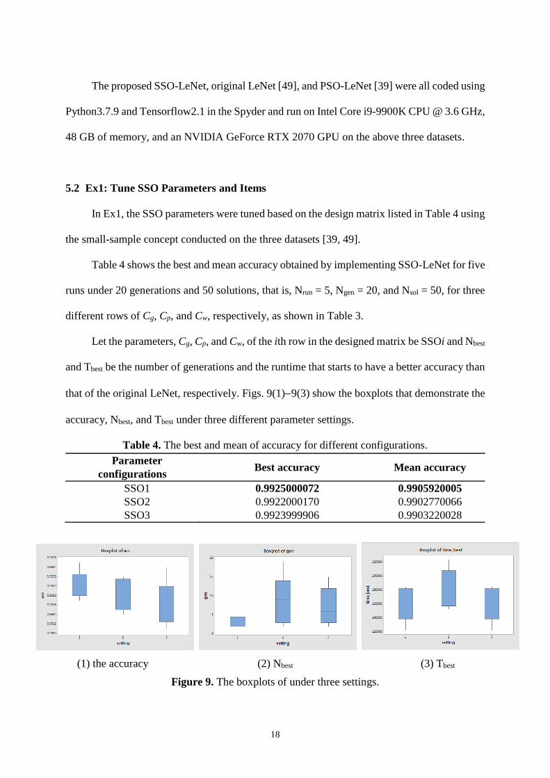
Let the parameters, Cg, Cp, and Cw, of the ith row in the designed matrix be SSOi and Nbest

and Tbest be the number of generations and the runtime that starts to have a better accuracy than

that of the original LeNet, respectively. Figs. 9(1)−9(3) show the boxplots that demonstrate the

accuracy, Nbest, and Tbest under three different parameter settings.

Table 4. The best and mean of accuracy for different configurations.

Parameter

configurations Best accuracy Mean accuracy

SSO1 0.9925000072 0.9905920005

SSO2 0.9922000170 0.9902770066

SSO3 0.9923999906 0.9903220028

(1) the accuracy (2) Nbest (3) Tbest

Figure 9. The boxplots of under three settings.

19

From Table 4 and Fig. 9, the first row, that is, (Cg, Cp, Cw) = (0.4, 0.7, 0.9), has the best

accuracy, mean accuracy, Nbest, and Tbest. In addition, the ranges of accuracy, Nbest, and Tbest are

more stable than the others, as shown in Fig. 9.

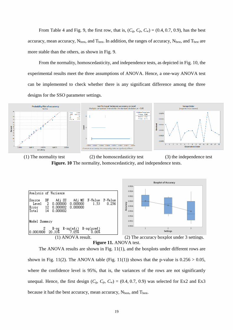
From the normality, homoscedasticity, and independence tests, as depicted in Fig. 10, the

experimental results meet the three assumptions of ANOVA. Hence, a one-way ANOVA test

can be implemented to check whether there is any significant difference among the three

designs for the SSO parameter settings.

(1) The normality test (2) the homoscedasticity test (3) the independence test

Figure. 10 The normality, homoscedasticity, and independence tests.

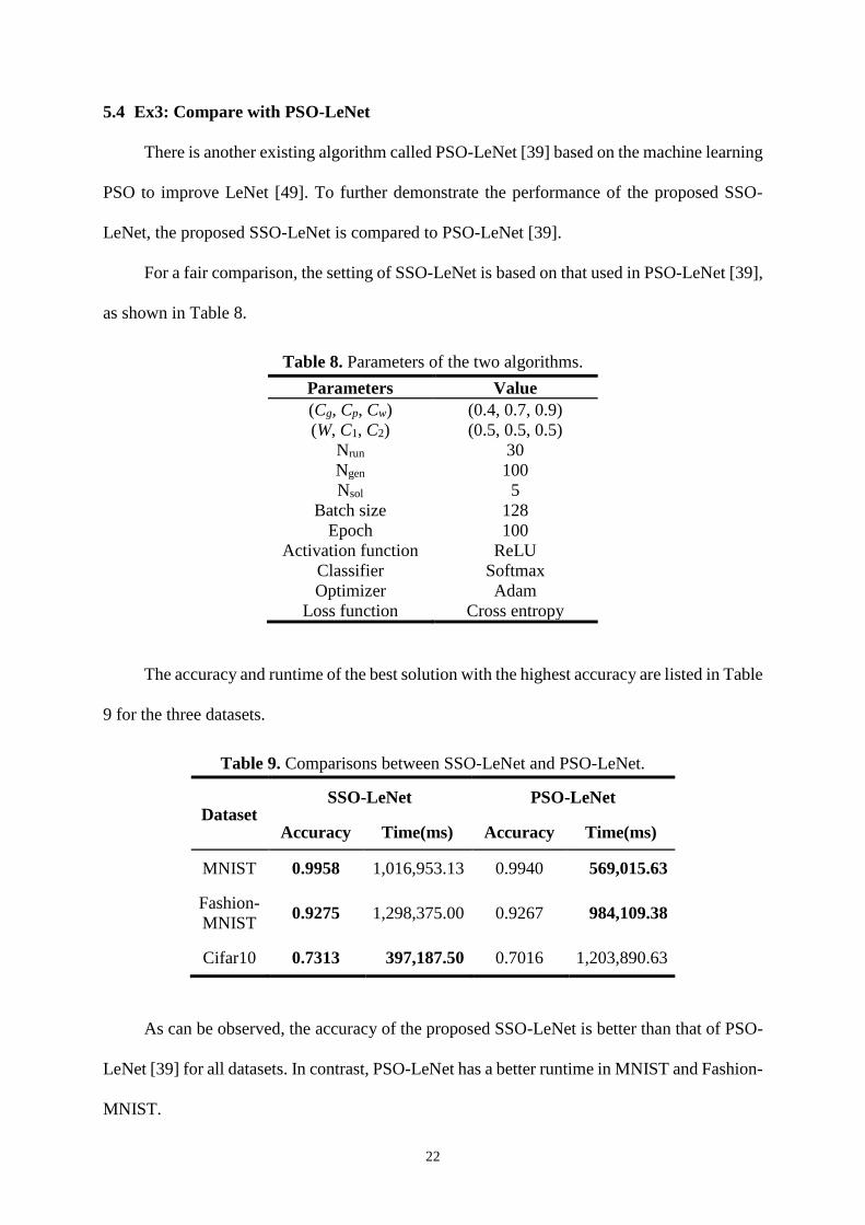
(1) ANOVA result. (2) The accuracy boxplot under 3 settings.

Figure 11. ANOVA test.

The ANOVA results are shown in Fig. 11(1), and the boxplots under different rows are

shown in Fig. 11(2). The ANOVA table (Fig. 11(1)) shows that the p-value is 0.256 > 0.05,

where the confidence level is 95%, that is, the variances of the rows are not significantly

unequal. Hence, the first design (Cg, Cp, Cw) = (0.4, 0.7, 0.9) was selected for Ex2 and Ex3

because it had the best accuracy, mean accuracy, Nbest, and Tbest.

321

0.9926

0.9924

0.9922

0.9920

0.9918

0.9916

0.9914

0.9912

0.9910

Settings

Accu

racy

Boxplot of Accuracy

20

5.3 Ex2: Compare to LeNet

Ex2 was conducted to validate whether there is an improvement in LeNet after using the

proposed SSO-LeNet. According to the results in Section 5.1, the best parameters (Cg, Cp, Cw)

= (0.4, 0.7, 0.9) were adopted in Ex2, and the other settings are summarised in Table 5.

Table 5. Summary of parameters

Parameter Value

(Cg, Cp, Cw) (0.4, 0.7, 0.9)

Nrun 30

Ngen 20 or the generation of which accuracy is larger

than that of LeNet

Nsol 30

Epoch 10

Activation function ReLU

Classifier Softmax

Optimizer the Stochastic Gradient Descent (SGD)

Loss function Cross entropy

The maximal accuracy Fmax, minimum accuracy Fmin, mean accuracy Fmean, standard

deviation of accuracy Fstd, mean testing runtime Ttest, and total training runtime Ttrain obtained

from the original LeNet and the proposed SSO-LeNet for the three datasets are listed in Table

6.

Table 6. The results of the dataset.

Dataset Method Fmax Fmin Fmean Fstd Ttest Ttrain

MNIST LeNet 0.9918 0.9876 0.9899 0.0009 203982.81 6119484.375

SSO-LeNet 0.9923 0.9891 0.9905 0.0008 172894.79 916772812.5

Fashion- LeNet 0.9005 0.8917 0.9001 0.0036 219691.15 6590734.38

MNIST SSO-LeNet 0.9113 0.8933 0.9021 0.0039 192489.50 1229022948

Cifar10 LeNet 0.6925 0.6596 0.6769 0.0092 2181456.25 65443687.5

SSO-LeNet 0.6951 0.6601 0.6807 0.0079 1899773.44 16671130781

From Table 6, it can be observed that all values obtained from SSO-LeNet are better than

those from LeNet except Ttrain for all datasets and Fstd for MNIST. However, the difference

between Fstd and MNIST was less than 0.003. In addition, it gives full play to the idea that fiscal

21

reserves should be used when the occasion calls for it, that is, the time taken for testing is more

important than that for training.

Hence, the proposed SSO-LeNet improves these two values in terms of accuracy and

runtime.

An interesting phenomenon is that the kernel in the best solution is not always a square

matrix. In general, each kernel (filter) is a square matrix in a CNN. However, Table 7 shows

that all input images have a square shape initially, that is, all runs have a square shape for the

three datasets. After performing more convolution and pooling layers for each generation in the

proposed SSO-LeNet, the size of the output feature map is close to a rectangle such that its

number of columns (i.e., the y-axis size of kernels) is less than that of rows (i.e., the x-axis size

of kernels), for example, 18 out of 30 runs with y < x for the MNIST. The above phenomenon

can be used to improve the convergence rate of the proposed SSO-LeNet in the future.

Table 7. Output size of the feature maps.

Dataset Size* Input Image C1# output P1

& output C2 output P2 output

MNIST x>y 0 11 20 18 18

x<y 0 16 10 12 11

x=y 30 3 0 0 1

Fashion- x>y 0 16 24 23 22

MNIST x<y 0 7 3 3 4

x=y 30 7 3 4 4

Cifar10 x>y 0 11 24 25 24

x<y 0 11 3 3 5

x=y 30 8 3 2 1 *: The x-axis and y-axis sizes of kernels denote by x and y, respectively. #: Ci is the ith convolution layer. #: Pi is the ith pooling layer.

22

5.4 Ex3: Compare with PSO-LeNet

There is another existing algorithm called PSO-LeNet [39] based on the machine learning

PSO to improve LeNet [49]. To further demonstrate the performance of the proposed SSO-

LeNet, the proposed SSO-LeNet is compared to PSO-LeNet [39].

For a fair comparison, the setting of SSO-LeNet is based on that used in PSO-LeNet [39],

as shown in Table 8.

Table 8. Parameters of the two algorithms.

Parameters Value

(Cg, Cp, Cw) (0.4, 0.7, 0.9)

(W, C1, C2) (0.5, 0.5, 0.5)

Nrun 30

Ngen 100

Nsol 5

Batch size 128

Epoch 100

Activation function ReLU

Classifier Softmax

Optimizer Adam

Loss function Cross entropy

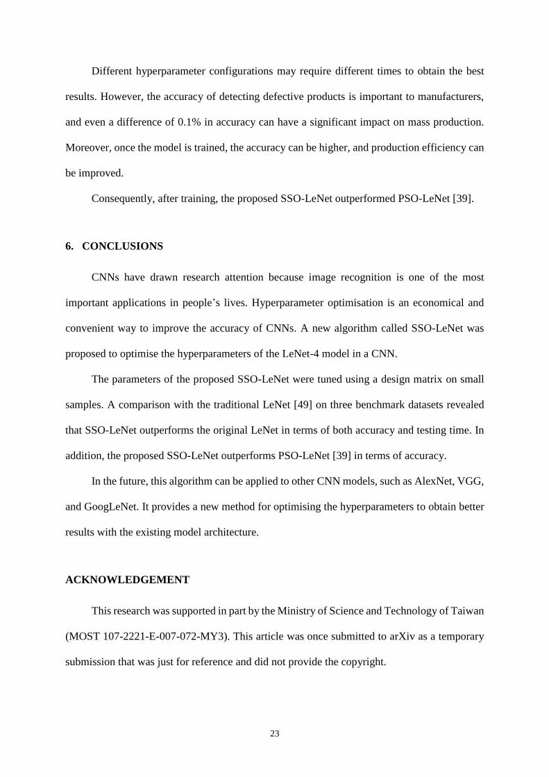
The accuracy and runtime of the best solution with the highest accuracy are listed in Table

9 for the three datasets.

Table 9. Comparisons between SSO-LeNet and PSO-LeNet.

Dataset SSO-LeNet PSO-LeNet

Accuracy Time(ms) Accuracy Time(ms)

MNIST 0.9958 1,016,953.13 0.9940 569,015.63

Fashion-

MNIST 0.9275 1,298,375.00 0.9267 984,109.38

Cifar10 0.7313 397,187.50 0.7016 1,203,890.63

As can be observed, the accuracy of the proposed SSO-LeNet is better than that of PSO-

LeNet [39] for all datasets. In contrast, PSO-LeNet has a better runtime in MNIST and Fashion-

MNIST.

23

Different hyperparameter configurations may require different times to obtain the best

results. However, the accuracy of detecting defective products is important to manufacturers,

and even a difference of 0.1% in accuracy can have a significant impact on mass production.

Moreover, once the model is trained, the accuracy can be higher, and production efficiency can

be improved.

Consequently, after training, the proposed SSO-LeNet outperformed PSO-LeNet [39].

6. CONCLUSIONS

CNNs have drawn research attention because image recognition is one of the most

important applications in people’s lives. Hyperparameter optimisation is an economical and

convenient way to improve the accuracy of CNNs. A new algorithm called SSO-LeNet was

proposed to optimise the hyperparameters of the LeNet-4 model in a CNN.

The parameters of the proposed SSO-LeNet were tuned using a design matrix on small

samples. A comparison with the traditional LeNet [49] on three benchmark datasets revealed

that SSO-LeNet outperforms the original LeNet in terms of both accuracy and testing time. In

addition, the proposed SSO-LeNet outperforms PSO-LeNet [39] in terms of accuracy.

In the future, this algorithm can be applied to other CNN models, such as AlexNet, VGG,

and GoogLeNet. It provides a new method for optimising the hyperparameters to obtain better

results with the existing model architecture.

ACKNOWLEDGEMENT

This research was supported in part by the Ministry of Science and Technology of Taiwan

(MOST 107-2221-E-007-072-MY3). This article was once submitted to arXiv as a temporary

submission that was just for reference and did not provide the copyright.

24

REFERENCES

[1] Krizhevsky, A.; Sutskever, I.; Hinton, G.E.: Imagenet classification with deep

convolutional neural networks. Advances in neural information processing systems

(2012), 1097-1105.

[2] Chen, K.; Huang, X.: Feature extraction method of 3D art creation based on deep learning.

Soft Computing (2019), 1-13.

[3] Chen, L.-C.; Papandreou, G.; Kokkinos, I.; Murphy, K.; Yuille, A.L.: Deeplab: Semantic

image segmentation with deep convolutional nets, atrous convolution, and fully

connected crfs. IEEE transactions on pattern analysis and machine intelligence, 40 (4)

(2017), 834-848.

[4] Loller-Andersen, M.; Gambäck, B.: ‘Deep Learning-based Poetry Generation Given

Visual Input, ICCC, 2018.

[5] LeCun, Y.; Bengio, Y.; Hinton, G.: Deep learning. Nature, 521 (7553) (2015), 436-444.

[6] Goodfellow, I.; Bengio, Y.; Courville, A.; Bengio, Y.: Deep learning, MIT Press

Cambridge, 2016.

[7] Al-Qizwini, M.; Barjasteh, I.; Al-Qassab, H.; Radha, H.: ‘Deep learning algorithm for

autonomous driving using googlenet, 2017 IEEE Intelligent Vehicles Symposium (IV),

2017.

[8] Miotto, R.; Wang, F.; Wang, S.; Jiang, X.; Dudley, J.T.: Deep learning for healthcare:

review, opportunities and challenges. Briefings in bioinformatics, 19 (6) (2018), 1236-

1246.

[9] Wang, T.; Chen, Y.; Qiao, M.; Snoussi, H.: A fast and robust convolutional neural

network-based defect detection model in product quality control. The International

Journal of Advanced Manufacturing Technology, 94 (9-12) (2018), 3465-3471.

[10] Lundervold, A.S.; Lundervold, A.: An overview of deep learning in medical imaging

focusing on MRI. Zeitschrift für Medizinische Physik, 29 (2) (2019), 102-127.

[11] Suzuki, K.: Overview of deep learning in medical imaging. Radiological physics and

technology, 10 (3) (2017), 257-273.

[12] Sultana, F.; Sufian, A.; Dutta, P.: ‘Advancements in image classification using

convolutional neural network, 2018 Fourth International Conference on Research in

Computational Intelligence and Communication Networks (ICRCICN), 2018.

[13] Bergstra, J.; Bardenet, R.; Bengio, Y.; Kégl, B.: Algorithms for hyper-parameter

optimization. Advances in neural information processing systems, 24 (2011), 2546-2554.

[14] Hubel, D.H.; Wiesel, T.N.: Receptive fields, binocular interaction and functional

architecture in the cat's visual cortex. The Journal of Physiology, 160 (1) (1962), 106.

[15] LeCun, Y.; Boser, B.; Denker, J.S.; Henderson, D.; Howard, R.E.; Hubbard, W.; Jackel,

L.D.: Backpropagation applied to handwritten zip code recognition. Neural computation,

1 (4) (1989), 541-551.

[16] Simonyan, K.; Zisserman, A.: Very deep convolutional networks for large-scale image

recognition. arXiv preprint arXiv:1409.1556 (2014)

[17] Szegedy, C.; Liu, W.; Jia, Y.; Sermanet, P.; Reed, S.; Anguelov, D.; Erhan, D.;

Vanhoucke, V.; Rabinovich, A.: ‘Going deeper with convolutions, Proceedings of the

IEEE conference on computer vision and pattern recognition, 2015.

[18] Ioffe, S.; Szegedy, C.: Batch normalization: Accelerating deep network training by

reducing internal covariate shift. arXiv preprint arXiv:1502.03167 (2015)

[19] Szegedy, C.; Vanhoucke, V.; Ioffe, S.; Shlens, J.; Wojna, Z.: ‘Rethinking the inception

architecture for computer vision, Proceedings of the IEEE conference on computer vision

and pattern recognition, 2016.

[20] Szegedy, C.; Ioffe, S.; Vanhoucke, V.; Alemi, A.: ‘Inception-v4, inception-resnet and the

impact of residual connections on learning, Proceedings of the AAAI Conference on

25

Artificial Intelligence, 2017.

[21] He, K.; Zhang, X.; Ren, S.; Sun, J.: ‘Deep residual learning for image recognition,

Proceedings of the IEEE conference on computer vision and pattern recognition, 2016.

[22] Hazan, E.; Klivans, A.; Yuan, Y.: Hyperparameter optimization: A spectral approach.

arXiv preprint arXiv:1706.00764 (2017)

[23] Zhang, X.; Chen, X.-C.; Yao, L.; Ge, C.; Dong, M.: ‘Deep neural network hyperparameter

optimization with orthogonal array tuning, International Conference on Neural

Information Processing, 2019.

[24] Salimans, T.; Kingma, D.P.: Weight normalization: A simple reparameterization to

accelerate training of deep neural networks. arXiv preprint arXiv:1602.07868 (2016)

[25] Cheng, D.; Gong, Y.; Zhou, S.; Wang, J.; Zheng, N.: ‘Person re-identification by multi-

channel parts-based cnn with improved triplet loss function, Proceedings of the iEEE

conference on computer vision and pattern recognition, 2016.

[26] Zhu, Q.-Y.; Zhang, P.-J.; Wang, Z.-Y.; Ye, X.: A New Loss Function for CNN Classifier

Based on Predefined Evenly-Distributed Class Centroids. IEEE Access, 8 (2019), 10888-

10895.

[27] Bergstra, J.; Bengio, Y.: Random search for hyper-parameter optimization. Journal of

machine learning research, 13 (2) (2012)

[28] Injadat, M.; Moubayed, A.; Nassif, A.B.; Shami, A.: Systematic ensemble model

selection approach for educational data mining. Knowledge-Based Systems, 200 (2020),

105992.

[29] Hinton, G.E.: A practical guide to training restricted Boltzmann machines, Neural

networks: Tricks of the trade, Springer, 2012, 599-619.

[30] Hsu, C.-W.; Chang, C.-C.; Lin, C.-J.: A practical guide to support vector classification.

(2003).

[31] Lemley, J.; Jagodzinski, F.; Andonie, R.: ‘Big holes in big data: A monte carlo algorithm

for detecting large hyper-rectangles in high dimensional data, 2016 IEEE 40th annual

computer software and applications conference (COMPSAC), 2016.

[32] Snoek, J.; Larochelle, H.; Adams, R.P.: Practical bayesian optimization of machine

learning algorithms. arXiv preprint arXiv:1206.2944 (2012)

[33] Shahriari, B.; Swersky, K.; Wang, Z.; Adams, R.P.; De Freitas, N.: Taking the human out

of the loop: A review of Bayesian optimization. Proceedings of the IEEE, 104 (1) (2015),

148-175.

[34] Aszemi, N.M.; Dominic, P.: Hyperparameter optimization in convolutional neural

network using genetic algorithms. Int. J. Adv. Comput. Sci. Appl., 10 (6) (2019), 269-

278.

[35] Johnson, F.; Valderrama, A.; Valle, C.; Crawford, B.; Soto, R.; Ñ anculef, R.: Automating

configuration of convolutional neural network hyperparameters using genetic algorithm.

IEEE Access, 8 (2020), 156139-156152.

[36] Loussaief, S.; Abdelkrim, A.: Convolutional neural network hyper-parameters

optimization based on genetic algorithms. International Journal of Advanced Computer

Science and Applications, 9 (10) (2018), 252-266.

[37] Xiao, X.; Yan, M.; Basodi, S.; Ji, C.; Pan, Y.: Efficient Hyperparameter Optimization in

Deep Learning Using a Variable Length Genetic Algorithm. arXiv preprint

arXiv:2006.12703 (2020)

[38] Huang, C.-L.: A particle-based simplified swarm optimization algorithm for reliability

redundancy allocation problems. Reliability Engineering & System Safety, 142 (2015),

221-230.

[39] Lorenzo, P.R.; Nalepa, J.; Kawulok, M.; Ramos, L.S.; Pastor, J.R.: ‘Particle swarm

optimization for hyper-parameter selection in deep neural networks, Proceedings of the

26

genetic and evolutionary computation conference, 2017.

[40] Yamasaki, T.; Honma, T.; Aizawa, K.: ‘Efficient optimization of convolutional neural

networks using particle swarm optimization, 2017 IEEE Third International Conference

on Multimedia Big Data (BigMM), 2017.

[41] Zhu, W.-B.; Yeh, W.-C.; Chen, J.-W.; Chen, D.-F.; Li, A.-Y.; Lin, Y.-Y.: ‘Evolutionary

convolutional neural networks using ABC, Proceedings of the 2019 11th International

Conference on Machine Learning and Computing, 2019.

[42] Yeh, W.-C.: Novel swarm optimization for mining classification rules on thyroid gland

data. Information Sciences, 197 (2012), 65-76.

[43] Yeh, W.-C.: Simplified swarm optimization in disassembly sequencing problems with

learning effects. Computers & Operations Research, 39 (9) (2012), 2168-2177.

[44] Yeh, W.-C.: Optimization of the disassembly sequencing problem on the basis of self-

adaptive simplified swarm optimization. IEEE transactions on systems, man, and

cybernetics-part A: systems and humans, 42 (1) (2011), 250-261.

[45] Yeh, W.-C.: Orthogonal simplified swarm optimization for the series–parallel

redundancy allocation problem with a mix of components. Knowledge-Based Systems,

64 (2014), 1-12.

[46] Yeh, W.-C.; Yeh, Y.-M.; Chou, C.-H.; Chung, Y.-Y.; He, X.: ‘A radio frequency

identification network design methodology for the decision problem in Mackay Memorial

Hospital based on swarm optimization, 2012 IEEE Congress on Evolutionary

Computation, 2012.

[47] Glorot, X.; Bordes, A.; Bengio, Y.: ‘Deep sparse rectifier neural networks, Proceedings

of the fourteenth international conference on artificial intelligence and statistics, 2011.

[48] Nair, V.; Hinton, G.E.: ‘Rectified linear units improve restricted boltzmann machines,

ICML, 2010.

[49] LeCun, Y.; Boser, B.E.; Denker, J.S.; Henderson, D.; Howard, R.E.; Hubbard, W.E.;

Jackel, L.D.: ‘Handwritten digit recognition with a back-propagation network, Advances

in neural information processing systems, 1990.

[50] LeCun, Y.; Bottou, L.; Bengio, Y.; Haffner, P.: Gradient-based learning applied to

document recognition. Proceedings of the IEEE, 86 (11) (1998), 2278-2324.

[51] Yeh, W.-C.: A two-stage discrete particle swarm optimization for the problem of multiple

multi-row redundancy allocation in series systems. Expert Systems with Applications, 36

(5) (2009), 9192-9200.

[52] Yeh, W.-C.; Chang, W.-W.; Chung, Y.Y.: A new hybrid approach for mining breast

cancer pattern using discrete particle swarm optimization and statistical method. Expert

Systems with Applications, 36 (4) (2009), 8204-8211.