convolutional neural networks analyzed via convolutional …€¦ · 2.1 deep learning -...
TRANSCRIPT
Journal of Machine Learning Research 18 (2017) 1-52 Submitted 10/16; Revised 6/17; Published 7/17
Convolutional Neural Networks Analyzed viaConvolutional Sparse Coding
Vardan Papyan* [email protected] of Computer ScienceTechnion - Israel Institute of TechnologyTechnion City, Haifa 32000, Israel
Yaniv Romano* [email protected] of Electrical EngineeringTechnion - Israel Institute of TechnologyTechnion City, Haifa 32000, Israel
Michael Elad [email protected]
Department of Computer Science
Technion - Israel Institute of Technology
Technion City, Haifa 32000, Israel
Editor: Kevin Murphy
Abstract
Convolutional neural networks (CNN) have led to many state-of-the-art results spanningthrough various fields. However, a clear and profound theoretical understanding of theforward pass, the core algorithm of CNN, is still lacking. In parallel, within the wide field ofsparse approximation, Convolutional Sparse Coding (CSC) has gained increasing attentionin recent years. A theoretical study of this model was recently conducted, establishing it asa reliable and stable alternative to the commonly practiced patch-based processing. Herein,we propose a novel multi-layer model, ML-CSC, in which signals are assumed to emergefrom a cascade of CSC layers. This is shown to be tightly connected to CNN, so much sothat the forward pass of the CNN is in fact the thresholding pursuit serving the ML-CSCmodel. This connection brings a fresh view to CNN, as we are able to attribute to thisarchitecture theoretical claims such as uniqueness of the representations throughout thenetwork, and their stable estimation, all guaranteed under simple local sparsity conditions.Lastly, identifying the weaknesses in the above pursuit scheme, we propose an alternativeto the forward pass, which is connected to deconvolutional and recurrent networks, andalso has better theoretical guarantees.
Keywords: Deep Learning, Convolutional Neural Networks, Forward Pass, Sparse Rep-resentation, Convolutional Sparse Coding, Thresholding Algorithm, Basis Pursuit
∗. The authors contributed equally to this work.
c©2017 Vardan Papyan, Yaniv Romano and Michael Elad.
License: CC-BY 4.0, see https://creativecommons.org/licenses/by/4.0/. Attribution requirements are providedat http://jmlr.org/papers/v18/16-505.html.
Papyan, Romano and Elad
1. Introduction
Deep learning (LeCun et al., 2015), and in particular CNN (LeCun et al., 1990, 1998;Krizhevsky et al., 2012), has gained a copious amount of attention in recent years as ithas led to many state-of-the-art results spanning through many fields – including speechrecognition (Bengio et al., 2003; Hinton et al., 2012; Mikolov et al., 2013), computer vision(Farabet et al., 2013; Simonyan and Zisserman, 2014; He et al., 2015), signal and imageprocessing (Gatys et al., 2015; Ulyanov et al., 2016; Johnson et al., 2016; Dong et al., 2016),to name a few. In the context of CNN, the forward pass is a multi-layer scheme that providesan end-to-end mapping, from an input signal to some desired output. Each layer of thisalgorithm consists of three steps. The first convolves the input with a set of learned filters,resulting in a set of feature (or kernel) maps. These then undergo a point wise non-linearfunction, in a second step, often resulting in a sparse outcome (Glorot et al., 2011). A third(and optional) down-sampling step, termed pooling, is then applied on the result in order toreduce its dimensions. The output of this layer is then fed into another one, thus formingthe multi-layer structure, often termed forward pass.
Despite its marvelous empirical success, a clear and profound theoretical understandingof this scheme is still lacking. A few preliminary theoretical results were recently sug-gested. In (Mallat, 2012; Bruna and Mallat, 2013) the Scattering Transform was proposed,suggesting to replace the learned filters in the CNN with predefined Wavelet functions. In-terestingly, the features obtained from this network were shown to be invariant to varioustransformations such as translations and rotations. Other works have studied the propertiesof deep and fully connected networks under the assumption of independent identically dis-tributed random weights (Giryes et al., 2015; Saxe et al., 2013; Arora et al., 2014; Dauphinet al., 2014; Choromanska et al., 2015). In particular, in (Giryes et al., 2015) deep neuralnetworks were proven to preserve the metric structure of the input data as it propagatesthrough the layers of the network. This, in turn, was shown to allow a stable recovery ofthe data from the features obtained from the network.
Another prominent paradigm in data processing is the sparse representation concept,being one of the most popular choices for a prior in the signal and image processing commu-nities, and leading to exceptional results in various applications (Elad and Aharon, 2006;Dong et al., 2011; Zhang and Li, 2010; Jiang et al., 2011; Mairal et al., 2014). In thisframework, one assumes that a signal can be represented as a linear combination of a fewcolumns (called atoms) from a matrix termed a dictionary. Put differently, the signal isequal to a multiplication of a dictionary by a sparse vector. The task of retrieving the spars-est representation of a signal over a dictionary is called sparse coding or pursuit. Over theyears, various algorithms were proposed to tackle this problem, among of which we mentionthe thresholding algorithm (Elad, 2010) and its iterative variant (Daubechies et al., 2004).When handling natural signals, this model has been commonly used for modeling localpatches extracted from the global data mainly due to the computational difficulties relatedto the task of learning the dictionary (Elad and Aharon, 2006; Dong et al., 2011; Mairalet al., 2014; Romano and Elad, 2015; Sulam and Elad, 2015). However, in recent yearsan alternative to this patch-based processing has emerged in the form of the ConvolutionalSparse Coding (CSC) model (Bristow et al., 2013; Kong and Fowlkes, 2014; Wohlberg, 2014;Gu et al., 2015; Heide et al., 2015; Papyan et al., 2016a,b). This circumvents the afore-
2
Convolutional Neural Networks Analyzed via Convolutional Sparse Coding
mentioned limitations by imposing a special structure – a union of banded and Circulantmatrices – on the dictionary involved. The traditional sparse model has been extensivelystudied over the past two decades (Elad, 2010; Foucart and Rauhut, 2013). More recently,the convolutional extension was extensively analyzed in (Papyan et al., 2016a,b), sheddinglight on its theoretical aspects and prospects of success.
In this work, by leveraging the recent study of CSC, we aim to provide a new perspec-tive on CNN, leading to a clear and profound theoretical understanding of this scheme,along with new insights. Embarking from the classic CSC, our approach builds upon theobservation that similar to the original signal, the representation vector itself also admits aconvolutional sparse representation. As such, it can be modeled as a superposition of atoms,taken from a different convolutional dictionary. This rationale can be extended to severallayers, leading to the definition of our proposed ML-CSC model. Building on the recentanalysis of the CSC, we provide a theoretical study of this novel model and its associatedpursuits, namely the layered thresholding algorithm and the layered basis pursuit (BP).
Our analysis reveals the relation between the CNN and the ML-CSC model, showingthat the forward pass of the CNN is in fact identical to our proposed pursuit – the layeredthresholding algorithm. This connection is of significant importance since it gives a clearmathematical meaning, objective and model to the CNN architecture, which in turn canbe accompanied by guarantees for the success of the forward pass, studied via the layeredthresholding algorithm. Specifically, we show that the forward pass is guaranteed to recoveran estimate of the underlying representations of an input signal, assuming these are sparsein a local sense. Moreover, considering a setting where a norm-bounded noise is addedto the signal, we show that such a mild corruption in the input results in a boundedperturbation in the output – indicating the stability of the CNN in recovering the underlyingrepresentations. Lastly, we exploit the answers to the above questions in order to proposean alternative to the commonly used forward pass algorithm, which is tightly connected toboth deconvolutional (Zeiler et al., 2010; Pu et al., 2016) and recurrent networks (Bengioet al., 1994). The proposed alternative scheme is accompanied by a thorough theoreticalstudy. Although this and the analysis presented throughout this work focus on CNN, wewill show that they also hold for fully connected networks.
This paper is organized as follows. In Section 2 we review the basics of both the CNN andthe Sparse-Land model. We then define the proposed ML-CSC model in Section 3, togetherwith its corresponding deep sparse coding problem. In Section 4, we aim to solve this usingthe layered thresholding algorithm, which is shown to be equivalent to the forward pass ofthe CNN. Next, having established the relevance of our model to CNN, we proceed to itsanalysis in Section 5. Standing on these theoretical grounds, we then propose in Section 6 aprovably improved pursuit, termed the layered BP, accompanied by its theoretical analysis.We revisit the assumptions of our model in Section 7. First, in Section 7.1 we link the doublesparsity model to ours by assuming the dictionaries throughout the layers are sparse. Then,in Section 7.2 we consider an idea typically employed in CNN, termed spatial-stride, showingits benefits from a simple theoretical perspective. Combining our insights from Section 7.1and 7.2, we move to an experimental phase by constructing a family of signals satisfyingthe assumptions of our model, which are then used in order to verify our theoretical results.Finally, in Section 9 we conclude the contributions of this paper and present several futuredirections.
3
Papyan, Romano and Elad
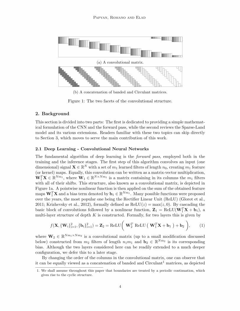
(a) A convolutional matrix.
(b) A concatenation of banded and Circulant matrices.
Figure 1: The two facets of the convolutional structure.
2. Background
This section is divided into two parts: The first is dedicated to providing a simple mathemat-ical formulation of the CNN and the forward pass, while the second reviews the Sparse-Landmodel and its various extensions. Readers familiar with these two topics can skip directlyto Section 3, which moves to serve the main contribution of this work.
2.1 Deep Learning - Convolutional Neural Networks
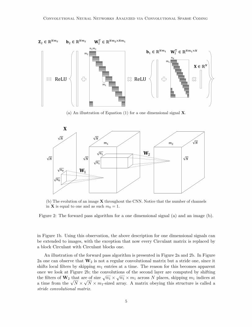
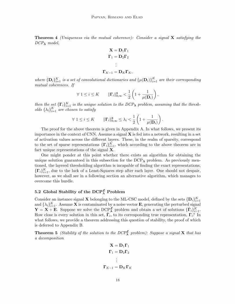
The fundamental algorithm of deep learning is the forward pass, employed both in thetraining and the inference stages. The first step of this algorithm convolves an input (onedimensional) signal X ∈ RN with a set of m1 learned filters of length n0, creating m1 feature(or kernel) maps. Equally, this convolution can be written as a matrix-vector multiplication,WT
1 X ∈ RNm1 , where W1 ∈ RN×Nm1 is a matrix containing in its columns the m1 filterswith all of their shifts. This structure, also known as a convolutional matrix, is depicted inFigure 1a. A pointwise nonlinear function is then applied on the sum of the obtained featuremaps WT
1 X and a bias term denoted by b1 ∈ RNm1 . Many possible functions were proposedover the years, the most popular one being the Rectifier Linear Unit (ReLU) (Glorot et al.,2011; Krizhevsky et al., 2012), formally defined as ReLU(z) = max(z, 0). By cascading thebasic block of convolutions followed by a nonlinear function, Z1 = ReLU(WT
1 X + b1), amulti-layer structure of depth K is constructed. Formally, for two layers this is given by
f(X, Wi2i=1, bi2i=1) = Z2 = ReLU
(WT
2 ReLU(
WT1 X + b1
)+ b2
), (1)
where W2 ∈ RNm1×Nm2 is a convolutional matrix (up to a small modification discussedbelow) constructed from m2 filters of length n1m1 and b2 ∈ RNm2 is its correspondingbias. Although the two layers considered here can be readily extended to a much deeperconfiguration, we defer this to a later stage.
By changing the order of the columns in the convolutional matrix, one can observe thatit can be equally viewed as a concatenation of banded and Circulant1 matrices, as depicted
1. We shall assume throughout this paper that boundaries are treated by a periodic continuation, whichgives rise to the cyclic structure.
4
Convolutional Neural Networks Analyzed via Convolutional Sparse Coding
𝑚1
𝐖2T ∈ ℝ𝑁𝑚2×𝑁𝑚1
𝐖1T ∈ ℝ𝑁𝑚1×𝑁
𝐗 ∈ ℝ𝑁
𝐛1 ∈ ℝ𝑁𝑚1
𝐛2 ∈ ℝ𝑁𝑚2𝐙2 ∈ ℝ
𝑁𝑚2
ReLU
𝑛1𝑚1
𝑚1
𝑛0
𝑚2
ReLU
(a) An illustration of Equation (1) for a one dimensional signal X.
𝑁
𝑁
𝐗
𝑚1
𝑁
𝑁
𝑛0
𝑛0 𝐖1
𝑚2 𝑁
𝑁
𝑛1
𝑛1
𝐖2
(b) The evolution of an image X throughout the CNN. Notice that the number of channelsin X is equal to one and as such m0 = 1.
Figure 2: The forward pass algorithm for a one dimensional signal (a) and an image (b).
in Figure 1b. Using this observation, the above description for one dimensional signals canbe extended to images, with the exception that now every Circulant matrix is replaced bya block Circulant with Circulant blocks one.
An illustration of the forward pass algorithm is presented in Figure 2a and 2b. In Figure2a one can observe that W2 is not a regular convolutional matrix but a stride one, since itshifts local filters by skipping m1 entries at a time. The reason for this becomes apparentonce we look at Figure 2b; the convolutions of the second layer are computed by shiftingthe filters of W2 that are of size
√n1 ×
√n1 ×m1 across N places, skipping m1 indices at
a time from the√N ×
√N ×m1-sized array. A matrix obeying this structure is called a
stride convolutional matrix.
5
Papyan, Romano and Elad
Thus far, we have presented the basic structure of CNN. However, oftentimes an ad-ditional non-linear function, termed pooling, is employed on the resulting feature map ob-tained from the ReLU operator. In essence, this step summarizes each wi-dimensionalspatial neighborhood from the i-th kernel map Zi by replacing it with a single value. Ifthe neighborhoods are non-overlapping, for example, this results in the down-sampling ofthe feature map by a factor of wi. The most widely used variant of the above is the maxpooling (Krizhevsky et al., 2012; Simonyan and Zisserman, 2014), which picks the maximalvalue of each neighborhood. In (Springenberg et al., 2014) it was shown that this operatorcan be replaced by a convolutional layer with increased stride without loss in performancein several image classification tasks. Moreover, the current state-of-the-art in image recog-nition is obtained by the residual network (He et al., 2015), which does not employ anypooling steps (except for a single layer). As such, we defer the analysis of this operator toa follow-up work.
In the context of classification, for example, the output of the last layer is fed into asimple classifier that attempts to predict the label of the input signal X, denoted by h(X).Given a set of signals Xjj , the task of learning the parameters of the CNN – includingthe filters WiKi=1, the biases biKi=1 and the parameters of the classifier U – can beformulated as the following minimization problem
minWiKi=1,biKi=1,U
∑j
`(h(Xj),U, f
(Xj , WiKi=1, biKi=1
) ). (2)
This optimization task seeks for the set of parameters that minimize the mean of the lossfunction `, representing the price incurred when classifying the signal X incorrectly. Theinput for ` is the true label h(X) and the one estimated by employing the classifier definedby U on the final layer of the CNN given by f
(X, WiKi=1, biKi=1
). Similarly one can
tackle various other problems, e.g. regression or prediction.
In the remainder of this work we shall focus on the feature extraction process and assumethat the parameters of the CNN model are pre-trained and fixed. These, for example, couldhave been obtained by minimizing the above objective via the backpropagation algorithmand the stochastic gradient descent, as in the VGG network (Simonyan and Zisserman,2014).
2.2 Sparse-Land
This section presents an overview of the Sparse-Land model and its many extensions. Westart with the traditional sparse representation and the core problem it aims to solve, andthen proceed to its nonnegative variant. Next, we continue to the dictionary learning taskboth in the unsupervised and supervised cases. Finally, we describe the recent CSC model,which will lead us in the next section to the proposal of the ML-CSC model. This, in turn,will naturally connect the realm of sparsity to that of the CNN.
2.2.1 Sparse Representation
In the sparse representation model one assumes a signal X ∈ RN can be described as amultiplication of a matrix D ∈ RN×M , also called a dictionary, by a sparse vector Γ ∈ RM .
6
Convolutional Neural Networks Analyzed via Convolutional Sparse Coding
Equally, the signal X can be seen as a linear combination of a few columns from thedictionary D, coined atoms.
For a fixed dictionary, given a signal X, the task of recovering its sparsest representationΓ is called sparse coding, or simply pursuit, and it attempts to solve the following problem(Donoho and Elad, 2003; Tropp, 2004; Elad, 2010):
(P0) : minΓ‖Γ‖0 s.t. DΓ = X, (3)
where we have denoted by ‖Γ‖0 the number of non-zeros in Γ. The above has a convexrelaxation in the form of the Basis-Pursuit (BP) problem (Chen et al., 2001; Donoho andElad, 2003; Tropp, 2006), formally defined as
(P1) : minΓ‖Γ‖1 s.t. DΓ = X. (4)
Many questions arise from the above two defined problems. For instance, given a signal X,is its sparsest representation unique? Assuming that such a unique solution exists, can itbe recovered using practical algorithms such as the Orthogonal Matching Pursuit (OMP)(Chen et al., 1989; Pati et al., 1993) and the BP (Chen et al., 2001; Daubechies et al., 2004)?The answers to these questions were shown to be positive under the assumption that thenumber of non-zeros in the underlying representation is not too high and in particular less
than 12
(1 + 1
µ(D)
)(Donoho and Elad, 2003; Tropp, 2004; Donoho et al., 2006). The quantity
µ(D) is the mutual coherence of the dictionary D, being the maximal inner product of twoatoms extracted from it2. Formally, we can write
µ(D) = maxi 6=j|dTi dj |.
Tighter conditions, relying on sharper characterizations of the dictionary, were also sug-gested in the literature (Candes et al., 2006; Schnass and Vandergheynst, 2007; Candeset al., 2006; Candes and Tao, 2007). However, at this point, we shall not dwell on these.
One of the simplest approaches for tackling the P0 and P1 problems is via the hard andsoft thresholding algorithms, respectively. These operate by computing the inner productsbetween the signal X and all the atoms in D and then choosing the atoms correspondingto the highest responses. This can be described as solving, for some scalar β, the followingproblems:
minΓ
1
2‖Γ−DTX‖22 + β‖Γ‖0
for the P0, or
minΓ
1
2‖Γ−DTX‖22 + β‖Γ‖1, (5)
for the P1. The above are simple projection problems that admit a closed-form solution inthe form3 of Hβ(DTX) or Sβ(DTX), where we have defined the hard thresholding operator
2. Hereafter, we assume that the atoms are normalized to a unit `2 norm.3. The curious reader may identify the relation between the notations used here and the ones in the
previous subsection, which starts to reveal the relation between CNN and sparsity-inspired models. Thisconnection will be made clearer as we proceed to CSC.
7
Papyan, Romano and Elad
Hβ(·) by
Hβ(z) =
z, z < −β0, −β ≤ z ≤ βz, β < z,
and the soft thresholding operator Sβ(·) by
Sβ(z) =
z + β, z < −β0, −β ≤ z ≤ βz − β, β < z.
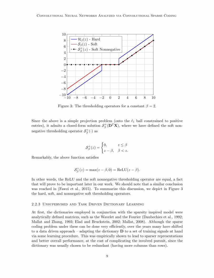
Both of the above, depicted in Figure 3, nullify small entries and thus promote a sparsesolution. However, while the hard thresholding operator does not modify large coefficients(in absolute value), the soft thresholding does, by contracting these to zero. This inherentlimitation of the soft version will appear later on in our theoretical analysis.
As for the theoretical guarantees for the success of the simple thresholding algorithms;these depend on the properties of D and on the ratio between the minimal and maximalcoefficients in absolute value in Γ, and thus are weaker when compared to those found forOMP and BP (Donoho and Elad, 2003; Tropp, 2004; Donoho et al., 2006). Still, undersome conditions, both algorithms are guaranteed to find the true support of Γ along withan approximation of its true coefficients. Moreover, a better estimation of these can beobtained by projecting the input signal onto the atoms corresponding to the found support(indices of the non-zero entries) by solving a Least-Squares problem. This step, termeddebiasing (Elad, 2010), results in a more accurate identification of the non-zero values.
2.2.2 Nonnegative Sparse Coding
The nonnegative sparse representation model assumes a signal can be decomposed into amultiplication of a dictionary and a nonnegative sparse vector. A natural question arisingfrom this is whether such a modification to the original Sparse-Land model affects its ex-pressiveness. To address this, we hereby provide a simple reduction from the original sparserepresentation to the nonnegative one.
Consider a signal X = DΓ, where the signs of the entries in Γ are unrestricted. Noticethat this can be equally written as
X = DΓP + (−D)(−ΓN ),
where we have split the vector Γ to its positive coefficients, ΓP , and its negative ones,ΓN . Since the coefficients in ΓP and −ΓN are all positive, one can thus assume the sig-nal X admits a non-negative sparse representation over the dictionary [D,−D] with thevector [ΓP ,−ΓN ]T . Thus, restricting the coefficients in the sparsity inspired model to benonnegative does not change its expressiveness.
Similar to the original model, in the nonnegative case, one could solve the associatedpursuit problem by employing a soft thresholding algorithm. However, in this case a con-straint must be added to the optimization problem in Equation (5), forcing the outcome tobe positive, i.e.,
minΓ
1
2‖Γ−DTX‖22 + β‖Γ‖1 s.t. Γ ≥ 0.
8
Convolutional Neural Networks Analyzed via Convolutional Sparse Coding
−10 −8 −6 −4 −2 0 2 4 6 8 10−10
−8
−6
−4
−2
0
2
4
6
8
10
Hβ(z) - Hard
Sβ(z) - Soft
S+β (z) - Soft Nonnegative
Figure 3: The thresholding operators for a constant β = 2.
Since the above is a simple projection problem (onto the `1 ball constrained to positiveentries), it admits a closed-form solution S+
β (DTX), where we have defined the soft non-
negative thresholding operator S+β (·) as
S+β (z) =
0, z ≤ βz − β, β < z.
Remarkably, the above function satisfies
S+β (z) = max(z − β, 0) = ReLU(z − β).
In other words, the ReLU and the soft nonnegative thresholding operator are equal, a factthat will prove to be important later in our work. We should note that a similar conclusionwas reached in (Fawzi et al., 2015). To summarize this discussion, we depict in Figure 3the hard, soft, and nonnegative soft thresholding operators.
2.2.3 Unsupervised and Task Driven Dictionary Learning
At first, the dictionaries employed in conjunction with the sparsity inspired model wereanalytically defined matrices, such as the Wavelet and the Fourier (Daubechies et al., 1992;Mallat and Zhang, 1993; Elad and Bruckstein, 2002; Mallat, 2008). Although the sparsecoding problem under these can be done very efficiently, over the years many have shiftedto a data driven approach – adapting the dictionary D to a set of training signals at handvia some learning procedure. This was empirically shown to lead to sparser representationsand better overall performance, at the cost of complicating the involved pursuit, since thedictionary was usually chosen to be redundant (having more columns than rows).
9
Papyan, Romano and Elad
The task of learning a dictionary for representing a set of signals Xjj can be formulatedas follows
minD,Γjj
∑j
‖Xj −DΓj‖22 + ξ‖Γj‖0.
The above formulation is an unsupervised learning procedure, and it was later extended toa supervised setting. In this context, given a set of signals Xjj , one attempts to predicttheir corresponding labels h(Xj)j . A common approach for tackling this is first solvinga pursuit problem for each signal Xj over a dictionary D, resulting in
Γ?(Xj ,D) = arg minΓ
‖Γ‖0 s.t. DΓ = Xj ,
and then feeding these sparse representations into a simple classifier, defined by the param-eters U. The task of learning jointly the dictionary D and the classifier U was addressedin (Mairal et al., 2012), where the following optimization problem was proposed
minD,U
∑j
`(h(Xj),U,Γ
?(Xj ,D)).
The loss function ` in the above objective penalizes the estimated label if it is differentfrom the true h(Xj), similar to what we have seen in Section 2.1. The above formulationcontains in it the unsupervised option as a special case, in which U is of no importance,and the loss function is the representation error
∑j ‖Xj −DΓ?j‖22.
Double sparsity – first proposed in (Rubinstein et al., 2010) and later employed in (Su-lam et al., 2016) – attempts to benefit from both the computational efficiency of analyticallydefined matrices, and the adaptability of data driven dictionaries. In this model, one as-sumes the dictionary D can be factorized into a multiplication of two matrices, D1 and D2,where D1 is an analytic dictionary with fast implementation, and D2 is a trained sparseone. As a result, the signal X can be represented as
X = DΓ2 = D1D2Γ2,
where Γ2 is sparse.
We propose a different interpretation for the above, which is unrelated to practicalaspects. Since both the matrix D2 and the vector Γ2 are sparse, one would expect theirmultiplication Γ1 = D2Γ2 to be sparse as well. As such, the double sparsity model implicitlyassumes that the signal X can be decomposed into a multiplication of a dictionary D1 andsparse vector Γ1, which in turn can also be decomposed similarly via Γ1 = D2Γ2.
2.2.4 Convolutional Sparse Coding Model
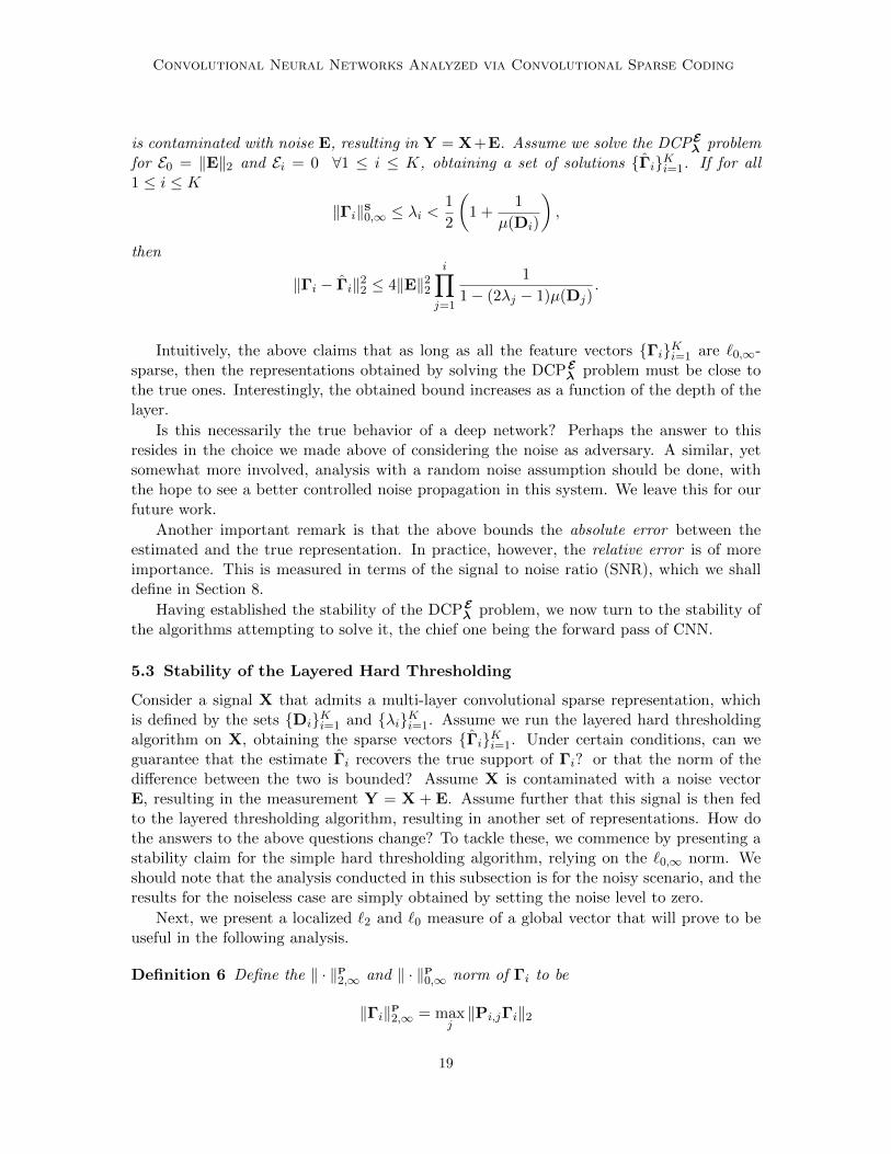
Due to the computational constraints entailed when deploying trained dictionaries, thisapproach seems valid only for treatment of low-dimensional signals. Indeed, the sparserepresentation model is traditionally used for modeling local patches extracted from a globalsignal. An alternative, which was recently proposed, is the CSC model that attempts torepresent the whole signal X ∈ RN as a multiplication of a global convolutional dictionaryD ∈ RN×Nm and a sparse vector Γ ∈ RNm. Interestingly, the former is constructed by
10
Convolutional Neural Networks Analyzed via Convolutional Sparse Coding
𝑚=
𝛀 ∈ ℝ𝑛× 2𝑛−1 𝑚
𝐱i ∈ ℝ𝑛 𝛄i ∈ ℝ
2𝑛−1 𝑚
𝑚
𝑛
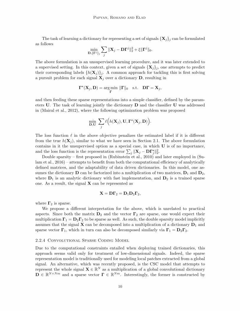
Figure 4: The i-th patch xi of the global system X = DΓ, given by xi = Ωγi.
shifting a local matrix of size n×m in all possible positions, resulting in the same structureas the one shown in Figure 1a.
In the convolutional model, the classical theoretical guarantees (we are referring toresults reported in (Chen et al., 2001; Donoho and Elad, 2003; Tropp, 2006)) for the P0
problem, defined in Equation (3), are very pessimistic. In particular, the condition for theuniqueness of the underlying solution and the requirement for the success of the sparse
coding algorithms depend on the global number of non-zeros being less than 12
(1 + 1
µ(D)
).
Following the Welch bound (Welch, 1974), this expression was shown in (Papyan et al.,2016a) to be impractical, allowing the global number of non-zeros in Γ to be extremely low.
In order to provide a better theoretical understanding of this model, which exploits theinherent structure of the convolutional dictionary, a recent work (Papyan et al., 2016a)suggested to measure the sparsity of Γ in a localized manner. More concretely, considerthe i-th n-dimensional patch of the global system X = DΓ, given by xi = Ωγi. The stripe-dictionary Ω, which is of size n× (2n− 1)m, is obtained by extracting the i-th patch fromthe global dictionary D and discarding all the zero columns from it. The stripe vector γiis the corresponding sparse representation of length (2n − 1)m, containing all coefficientsof atoms contributing to xi. This relation is illustrated in Figure 4. Notably, the choiceof a convolutional dictionary results in signals such that every patch of length n extractedfrom them can be sparsely represented using a single shift-invariant local dictionary Ω – acommon assumption usually employed in signal and image processing.
Following the above construction, the `0,∞ norm of the global sparse vector Γ is definedto be the maximal number of non-zeros in a stripe of length (2n − 1)m extracted from it.Formally,
‖Γ‖S0,∞ = maxi‖γi‖0,
where the letter s emphasizes that the `0,∞ norm is computed by sweeping over all stripes.Given a signal X, finding its sparest representation Γ in the `0,∞ sense is equal to thefollowing optimization problem:
(P0,∞) : minΓ
‖Γ‖S0,∞ s.t. DΓ = X. (6)
11
Papyan, Romano and Elad
Intuitively, this seeks for a global vector Γ that can represent sparsely every patch in thesignal X using the dictionary Ω. The advantage of the above problem over the traditionalP0 becomes apparent as we move to consider its theoretical aspects. Assuming that the
number of non-zeros per stripe (and not globally) in Γ is less than 12
(1 + 1
µ(D)
), in
(Papyan et al., 2016a) it was proven that the solution for the P0,∞ problem is unique.Furthermore, classical pursuit methods, originally tackling the P0 problem, are guaranteedto find this representation.
When modeling natural signals, due to measurement noise as well as model deviations,one can not impose a perfect reconstruction such as X = DΓ on the signal X. Instead, oneassumes Y = X + E = DΓ + E, where E is, for example, an `2-bounded error vector. Toaddress this, the work reported in (Papyan et al., 2016b) considered the extension of theP0,∞ problem to the PE
0,∞ one, formally defined as
(PE0,∞) : min
Γ‖Γ‖S0,∞ s.t. ‖Y −DΓ‖22 ≤ E2.
Similar to the P0,∞ problem, this was also analyzed theoretically, shedding light on thetheoretical aspects of the convolutional model in the presence of noise. In particular, astability claim for the PE
0,∞ problem and guarantees for the success of both the OMP andthe BP were provided. Similar to the noiseless case, these assumed that the number ofnon-zeros per stripe is low.
3. From Atoms to Molecules: Multi-Layer Convolutional Sparse Model
Convolutional sparsity assumes an inherent structure for natural signals. Similarly, therepresentations themselves could also be assumed to have such a structure. In what follows,we propose a novel layered model that relies on this rationale.
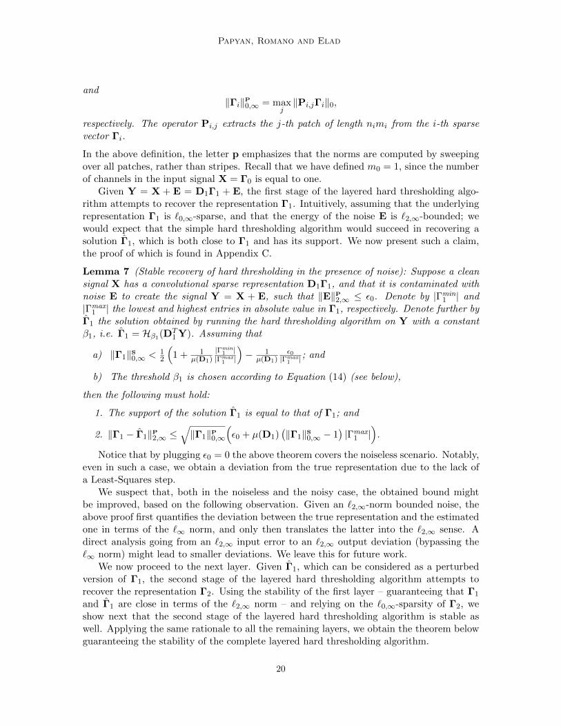
The convolutional sparse model assumes a global signal X ∈ RN can be decomposedinto a multiplication of a convolutional dictionary D1 ∈ RN×Nm1 , composed of m1 localfilters of length n0, and a sparse vector Γ1 ∈ RNm1 . Herein, we extend this by proposing asimilar factorization of the vector Γ1, which can be perceived as an N -dimensional globalsignal with m1 channels. In particular, we assume Γ1 = D2Γ2, where D2 ∈ RNm1×Nm2
is a stride convolutional dictionary (skipping m1 entries at a time) and Γ2 ∈ RNm2 is asparse representation. We denote the number of unique filters constructing D2 by m2 andtheir corresponding length by n1m1. Due to the multi-layer nature of this model and theimposed convolutional structure, we name this the ML-CSC model.
Intuitively, X = D1Γ1 assumes that the signal X is a superposition of atoms takenfrom D1. While equation X = D1D2Γ2 views the signal as a superposition of more complexentities taken from the dictionary D1D2, which we coin molecules.
While this proposal can be interpreted as a straightforward fusion between the doublesparsity model (Rubinstein et al., 2010) and the convolutional one, it is in fact substantiallydifferent. The double sparsity model assumes that D2 is sparse, and forces only the deepestrepresentation Γ2 to be sparse as well. Here, on the other hand, we replace this constraintby forcing D2 to have a stride convolution structure, putting emphasis on the sparsity ofboth the representations Γ1 and Γ2. In Section 7.1 we will revisit the double sparsity workand its ties to ours by showing the benefits of injecting the assumption on the sparsity ofD2 into our proposed model.
12
Convolutional Neural Networks Analyzed via Convolutional Sparse Coding
𝑚1
𝑛0
𝐃1 ∈ ℝ𝑁×𝑁𝑚1 𝚪1 ∈ ℝ
𝑁𝑚1𝐗 ∈ ℝ𝑁
𝚪1 ∈ ℝ𝑁𝑚1
𝑛1𝑚1
𝑚2
𝐒1,𝑗𝚪1 ∈ ℝ2𝑛0−1 𝑚1
𝐏1,𝑗𝚪1 ∈ ℝ𝑛1𝑚1
𝐃2 ∈ ℝ𝑁𝑚1×𝑁𝑚2 𝚪2 ∈ ℝ
𝑁𝑚2
𝑚1
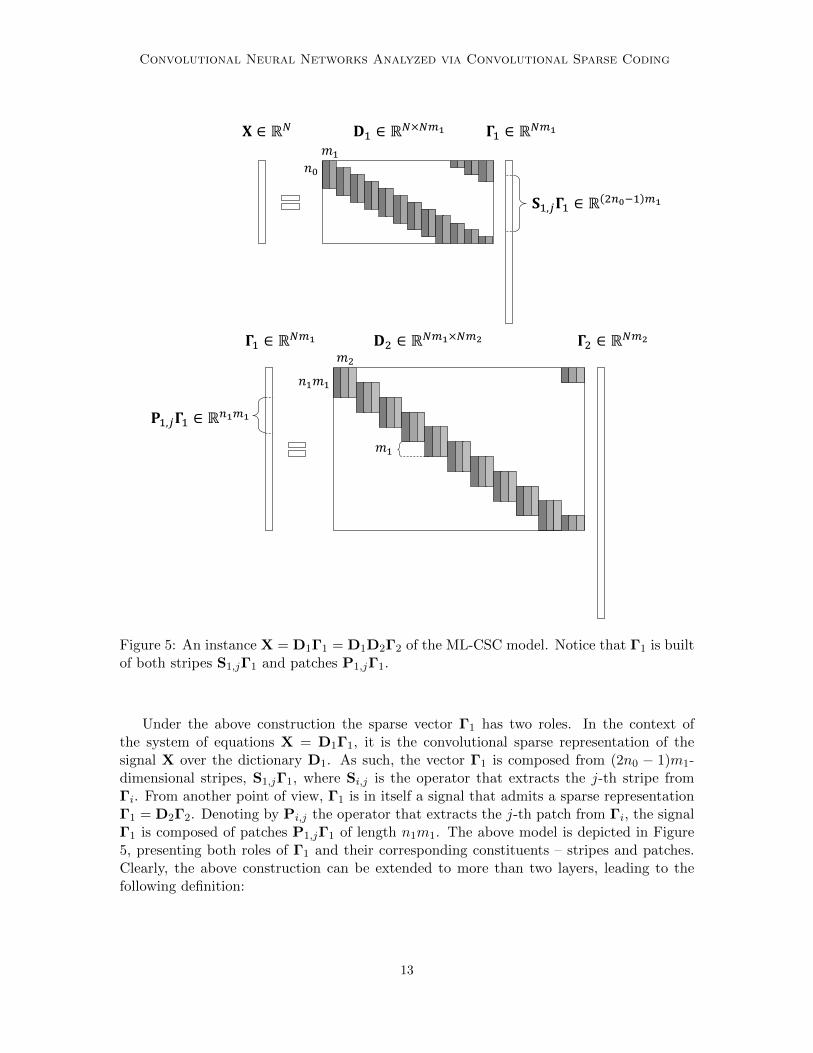
Figure 5: An instance X = D1Γ1 = D1D2Γ2 of the ML-CSC model. Notice that Γ1 is builtof both stripes S1,jΓ1 and patches P1,jΓ1.
Under the above construction the sparse vector Γ1 has two roles. In the context ofthe system of equations X = D1Γ1, it is the convolutional sparse representation of thesignal X over the dictionary D1. As such, the vector Γ1 is composed from (2n0 − 1)m1-dimensional stripes, S1,jΓ1, where Si,j is the operator that extracts the j-th stripe fromΓi. From another point of view, Γ1 is in itself a signal that admits a sparse representationΓ1 = D2Γ2. Denoting by Pi,j the operator that extracts the j-th patch from Γi, the signalΓ1 is composed of patches P1,jΓ1 of length n1m1. The above model is depicted in Figure5, presenting both roles of Γ1 and their corresponding constituents – stripes and patches.Clearly, the above construction can be extended to more than two layers, leading to thefollowing definition:
13
Papyan, Romano and Elad
Definition 1 For a global signal X, a set of convolutional dictionaries DiKi=1, and avector λ, define the deep coding problem DCPλ as:
(DCPλ) : find ΓiKi=1 s.t. X = D1Γ1, ‖Γ1‖S0,∞ ≤ λ1
Γ1 = D2Γ2, ‖Γ2‖S0,∞ ≤ λ2
......
ΓK−1 = DKΓK , ‖ΓK‖S0,∞ ≤ λK ,
where the scalar λi is the i-th entry of λ.
Denoting Γ0 to be the signal X, the DCPλ can be rewritten compactly as
(DCPλ) : find ΓiKi=1 s.t. Γi−1 = DiΓi, ‖Γi‖S0,∞ ≤ λi, ∀1 ≤ i ≤ K.
Intuitively, given a signal X, this problem seeks for a set of representations, ΓiKi=1, suchthat each one is locally sparse. As we shall see next, the above can be easily solved usingsimple algorithms that also enjoy from theoretical justifications. Next, we extend the DCPλ
problem to a noisy regime.
Definition 2 For a global signal Y, a set of convolutional dictionaries DiKi=1, and vectorsλ and E, define the deep coding problem DCPE
λ as:
(DCPEλ ) : find ΓiKi=1 s.t. ‖Y −D1Γ1‖2 ≤ E0, ‖Γ1‖S0,∞ ≤ λ1
‖Γ1 −D2Γ2‖2 ≤ E1, ‖Γ2‖S0,∞ ≤ λ2
......
‖ΓK−1 −DKΓK‖2 ≤ EK−1, ‖ΓK‖S0,∞ ≤ λK ,
where the scalars λi and Ei are the i-th entry of λ and E, respectively.
We now move to the task of learning the model parameters. Denote by DCP?λ(X, DiKi=1)
the representation ΓK obtained by solving the DCP problem (Definition 1, i.e., noiseless)for the signal X and the set of dictionaries DiKi=1. Relying on this, we now extend thedictionary learning problem, as presented in Section 2.2.3, to the multi-layer convolutionalsparse representation setting.
Definition 3 For a set of global signals Xjj, their corresponding labels h(Xj)j, a lossfunction `, and a vector λ, define the deep learning problem DLPλ as:
(DLPλ) : minDiKi=1,U
∑j
`(h(Xj),U,DCP?
λ(Xj , DiKi=1)).
A clarification for the chosen name, deep learning problem, will be provided shortly. Thesolution for the above results in an end-to-end mapping, from a set of input signals to theircorresponding labels. Similarly, we can define the DLPE
λ problem. However, this is omittedfor the sake of brevity. We conclude this section by summarizing, for the convenience of thereader, all notations used throughout this work in Table 1.
14
Convolutional Neural Networks Analyzed via Convolutional Sparse Coding
X = Γ0 : a global signal of length N .
E, Y = Γ0 : a global error vector and its corresponding noisy signal, where generallyY = X + E.
K : the number of layers.
mi : the number of local filters in Di, and also the number of channels in Γi.Notice that m0 = 1.
n0 : the size of a local patch in X = Γ0.
ni, i ≥ 1 : the size of a local patch (not including channels) in Γi.
nimi : the size of a local patch (including channels) in Γi.
D1 : a (full) convolutional dictionary of size N ×Nm1 with filters of length n0.
Di, i ≥ 2 : a convolutional dictionary of size Nmi−1 × Nmi with filters of lengthni−1mi−1 and a stride equal to mi−1.
Γi : a sparse vector of length Nmi that is the representation of Γi−1 over thedictionary Di, i.e. Γi−1 = DiΓi.
Si,j : an operator that extracts the j-th stripe of length (2ni−1 − 1)mi from Γi.
‖Γi‖S0,∞ : the maximal number of non-zeros in a stripe from Γi.
Pi,j : an operator that extracts the j-th nimi-dimensional patch from Γi.
‖Γi‖P0,∞ : the maximal number of non-zeros in a patch from Γi (Definition 6).
Ri,j : an operator that extracts the filter of length ni−1mi−1 from the j-th atomin Di.
‖V‖P2,∞ : the maximal `2 norm of a patch extracted from a vector V (Definition 6).
Table 1: Summary of notations used throughout the paper.
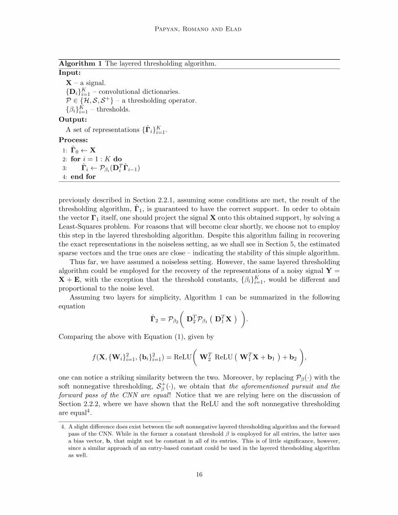
4. Layered Thresholding: The Crux of the Matter
Consider the ML-CSC model defined by the set of dictionaries DiKi=1. Assume we aregiven a signal
X = D1Γ1
Γ1 = D2Γ2
...
ΓK−1 = DKΓK ,
and our goal is to find its underlying representations, ΓiKi=1. Tackling this problem byrecovering all the vectors at once might be computationally and conceptually challenging;therefore, we propose the layered thresholding algorithm that gradually computes the sparsevectors one at a time across the different layers. Denoting by Pβ(·) a sparsifying operatorthat is equal to Hβ(·) in the hard thresholding case and Sβ(·) in the soft one; we commence
by computing Γ1 = Pβ1(DT1 X), which is an approximation of Γ1. Next, by applying another
thresholding algorithm, however this time on Γ1, an approximation of Γ2 is obtained, Γ2 =Pβ2(DT
2 Γ1). This process, which is iterated until the last representation ΓK is acquired, issummarized in Algorithm 1.
One might ponder as to why does the application of the thresholding algorithm on thesignal X not result in the true representation Γ1, but instead an approximation of it. As
15
Papyan, Romano and Elad
Algorithm 1 The layered thresholding algorithm.
Input:
X – a signal.DiKi=1 – convolutional dictionaries.P ∈ H,S,S+ – a thresholding operator.βiKi=1 – thresholds.
Output:
A set of representations ΓiKi=1.
Process:
1: Γ0 ← X2: for i = 1 : K do3: Γi ← Pβi(DT
i Γi−1)4: end for
previously described in Section 2.2.1, assuming some conditions are met, the result of thethresholding algorithm, Γ1, is guaranteed to have the correct support. In order to obtainthe vector Γ1 itself, one should project the signal X onto this obtained support, by solving aLeast-Squares problem. For reasons that will become clear shortly, we choose not to employthis step in the layered thresholding algorithm. Despite this algorithm failing in recoveringthe exact representations in the noiseless setting, as we shall see in Section 5, the estimatedsparse vectors and the true ones are close – indicating the stability of this simple algorithm.
Thus far, we have assumed a noiseless setting. However, the same layered thresholdingalgorithm could be employed for the recovery of the representations of a noisy signal Y =X + E, with the exception that the threshold constants, βiKi=1, would be different andproportional to the noise level.
Assuming two layers for simplicity, Algorithm 1 can be summarized in the followingequation
Γ2 = Pβ2(
DT2 Pβ1
(DT
1 X) )
.
Comparing the above with Equation (1), given by
f(X, Wi2i=1, bi2i=1) = ReLU
(WT
2 ReLU(
WT1 X + b1
)+ b2
),
one can notice a striking similarity between the two. Moreover, by replacing Pβ(·) with thesoft nonnegative thresholding, S+
β (·), we obtain that the aforementioned pursuit and theforward pass of the CNN are equal ! Notice that we are relying here on the discussion ofSection 2.2.2, where we have shown that the ReLU and the soft nonnegative thresholdingare equal4.
4. A slight difference does exist between the soft nonnegative layered thresholding algorithm and the forwardpass of the CNN. While in the former a constant threshold β is employed for all entries, the latter usesa bias vector, b, that might not be constant in all of its entries. This is of little significance, however,since a similar approach of an entry-based constant could be used in the layered thresholding algorithmas well.
16
Convolutional Neural Networks Analyzed via Convolutional Sparse Coding
Recall the optimization problem of the training stage of the CNN as shown in Equation(2), given by
minWiKi=1,biKi=1,U
∑j
`(h(Xj),U, f
(Xj , WiKi=1, biKi=1
) ),
and its parallel in the ML-CSC model, the DLPλ problem, defined by
minDiKi=1,U
∑j
`(h(Xj),U,DCP?
λ(Xj , DiKi=1)).
Notice the remarkable similarity between both objectives, the only difference being in thefeature vector on which the classification is done; in the CNN this is the output of theforward pass algorithm, given by f
(Xj , WiKi=1, biKi=1
), while in the sparsity case this is
the result of the DCPλ problem. In light of the discussion above, the solution for the DCPλ
problem can be approximated using the layered thresholding algorithm, which is in turnequal to the forward pass of the CNN. We can therefore conclude that the problems solvedby the training stage of the CNN and the DLPλ are tightly connected, and in fact are equalonce the solution for the DLPλ is approximated via the layered thresholding algorithm(hence the name DLPλ).
5. Theoretical Study
Thus far, we have defined the ML-CSC model and its corresponding pursuits – the DCPλ
and DCPEλ problems. We have proposed a method to tackle them, coined the layered thresh-
olding algorithm, which was shown to be equivalent to the forward pass of the CNN. Relyingon this, we conclude that the proposed ML-CSC is the global Bayesian model implicitlyimposed on the signal X when deploying the forward pass algorithm. Put differently, theML-CSC answers the question of who are the signals belonging to the model behind theCNN. Having established the importance of our model, we now proceed to its theoreticalanalysis.
We should emphasize that the following study does not assume any specific form on thenetwork’s parameters, apart from a broad coherence property (as will be shown hereafter).This is in contrast to the work of (Bruna and Mallat, 2013) that assumes that the filtersare Wavelets, or the analysis in (Giryes et al., 2015) that considers random weights.
5.1 Uniqueness of the DCPλ Problem
Consider a signal X admitting a multi-layer convolutional sparse representation defined bythe sets DiKi=1 and λiKi=1. Can another set of sparse vectors represent the signal X?In other words, can we guarantee that, under some conditions, the set ΓiKi=1 is a uniquesolution to the DCPλ problem? In the following theorem we provide an answer to thisquestion.
17
Papyan, Romano and Elad
Theorem 4 (Uniqueness via the mutual coherence): Consider a signal X satisfying theDCPλ model,
X = D1Γ1
Γ1 = D2Γ2
...
ΓK−1 = DKΓK ,
where DiKi=1 is a set of convolutional dictionaries and µ(Di)Ki=1 are their correspondingmutual coherences. If
∀ 1 ≤ i ≤ K ‖Γi‖S0,∞ <1
2
(1 +
1
µ(Di)
),
then the set ΓiKi=1 is the unique solution to the DCPλ problem, assuming that the thresh-olds λiKi=1 are chosen to satisfy
∀ 1 ≤ i ≤ K ‖Γi‖S0,∞ ≤ λi <1
2
(1 +
1
µ(Di)
).
The proof for the above theorem is given in Appendix A. In what follows, we present itsimportance in the context of CNN. Assume a signal X is fed into a network, resulting in a setof activation values across the different layers. These, in the realm of sparsity, correspondto the set of sparse representations ΓiKi=1, which according to the above theorem are infact unique representations of the signal X.
One might ponder at this point whether there exists an algorithm for obtaining theunique solution guaranteed in this subsection for the DCPλ problem. As previously men-tioned, the layered thresholding algorithm is incapable of finding the exact representations,ΓiKi=1, due to the lack of a Least-Squares step after each layer. One should not despair,however, as we shall see in a following section an alternative algorithm, which manages toovercome this hurdle.
5.2 Global Stability of the DCPEλ Problem
Consider an instance signal X belonging to the ML-CSC model, defined by the sets DiKi=1
and λiKi=1. Assume X is contaminated by a noise vector E, generating the perturbed signalY = X + E. Suppose we solve the DCPE
λ problem and obtain a set of solutions ΓiKi=1.How close is every solution in this set, Γi, to its corresponding true representation, Γi? Inwhat follows, we provide a theorem addressing this question of stability, the proof of whichis deferred to Appendix B.
Theorem 5 (Stability of the solution to the DCPEλ problem): Suppose a signal X that has
a decomposition
X = D1Γ1
Γ1 = D2Γ2
...
ΓK−1 = DKΓK
18
Convolutional Neural Networks Analyzed via Convolutional Sparse Coding
is contaminated with noise E, resulting in Y = X+E. Assume we solve the DCPEλ problem
for E0 = ‖E‖2 and Ei = 0 ∀1 ≤ i ≤ K, obtaining a set of solutions ΓiKi=1. If for all1 ≤ i ≤ K
‖Γi‖S0,∞ ≤ λi <1
2
(1 +
1
µ(Di)
),
then
‖Γi − Γi‖22 ≤ 4‖E‖22i∏
j=1
1
1− (2λj − 1)µ(Dj).
Intuitively, the above claims that as long as all the feature vectors ΓiKi=1 are `0,∞-sparse, then the representations obtained by solving the DCPE
λ problem must be close tothe true ones. Interestingly, the obtained bound increases as a function of the depth of thelayer.
Is this necessarily the true behavior of a deep network? Perhaps the answer to thisresides in the choice we made above of considering the noise as adversary. A similar, yetsomewhat more involved, analysis with a random noise assumption should be done, withthe hope to see a better controlled noise propagation in this system. We leave this for ourfuture work.
Another important remark is that the above bounds the absolute error between theestimated and the true representation. In practice, however, the relative error is of moreimportance. This is measured in terms of the signal to noise ratio (SNR), which we shalldefine in Section 8.
Having established the stability of the DCPEλ problem, we now turn to the stability of
the algorithms attempting to solve it, the chief one being the forward pass of CNN.
5.3 Stability of the Layered Hard Thresholding
Consider a signal X that admits a multi-layer convolutional sparse representation, whichis defined by the sets DiKi=1 and λiKi=1. Assume we run the layered hard thresholdingalgorithm on X, obtaining the sparse vectors ΓiKi=1. Under certain conditions, can weguarantee that the estimate Γi recovers the true support of Γi? or that the norm of thedifference between the two is bounded? Assume X is contaminated with a noise vectorE, resulting in the measurement Y = X + E. Assume further that this signal is then fedto the layered thresholding algorithm, resulting in another set of representations. How dothe answers to the above questions change? To tackle these, we commence by presenting astability claim for the simple hard thresholding algorithm, relying on the `0,∞ norm. Weshould note that the analysis conducted in this subsection is for the noisy scenario, and theresults for the noiseless case are simply obtained by setting the noise level to zero.
Next, we present a localized `2 and `0 measure of a global vector that will prove to beuseful in the following analysis.
Definition 6 Define the ‖ · ‖P2,∞ and ‖ · ‖P0,∞ norm of Γi to be
‖Γi‖P2,∞ = maxj‖Pi,jΓi‖2
19
Papyan, Romano and Elad
and‖Γi‖P0,∞ = max
j‖Pi,jΓi‖0,
respectively. The operator Pi,j extracts the j-th patch of length nimi from the i-th sparsevector Γi.
In the above definition, the letter p emphasizes that the norms are computed by sweepingover all patches, rather than stripes. Recall that we have defined m0 = 1, since the numberof channels in the input signal X = Γ0 is equal to one.
Given Y = X + E = D1Γ1 + E, the first stage of the layered hard thresholding algo-rithm attempts to recover the representation Γ1. Intuitively, assuming that the underlyingrepresentation Γ1 is `0,∞-sparse, and that the energy of the noise E is `2,∞-bounded; wewould expect that the simple hard thresholding algorithm would succeed in recovering asolution Γ1, which is both close to Γ1 and has its support. We now present such a claim,the proof of which is found in Appendix C.
Lemma 7 (Stable recovery of hard thresholding in the presence of noise): Suppose a cleansignal X has a convolutional sparse representation D1Γ1, and that it is contaminated withnoise E to create the signal Y = X + E, such that ‖E‖P2,∞ ≤ ε0. Denote by |Γmin
1 | and|Γmax
1 | the lowest and highest entries in absolute value in Γ1, respectively. Denote further byΓ1 the solution obtained by running the hard thresholding algorithm on Y with a constantβ1, i.e. Γ1 = Hβ1(DT
1 Y). Assuming that
a) ‖Γ1‖S0,∞ < 12
(1 + 1
µ(D1)|Γmin
1 ||Γmax
1 |
)− 1
µ(D1)ε0|Γmax
1 | ; and
b) The threshold β1 is chosen according to Equation (14) (see below),
then the following must hold:
1. The support of the solution Γ1 is equal to that of Γ1; and
2. ‖Γ1 − Γ1‖P2,∞ ≤√‖Γ1‖P0,∞
(ε0 + µ(D1)
(‖Γ1‖S0,∞ − 1
)|Γmax
1 |)
.
Notice that by plugging ε0 = 0 the above theorem covers the noiseless scenario. Notably,even in such a case, we obtain a deviation from the true representation due to the lack ofa Least-Squares step.
We suspect that, both in the noiseless and the noisy case, the obtained bound mightbe improved, based on the following observation. Given an `2,∞-norm bounded noise, theabove proof first quantifies the deviation between the true representation and the estimatedone in terms of the `∞ norm, and only then translates the latter into the `2,∞ sense. Adirect analysis going from an `2,∞ input error to an `2,∞ output deviation (bypassing the`∞ norm) might lead to smaller deviations. We leave this for future work.
We now proceed to the next layer. Given Γ1, which can be considered as a perturbedversion of Γ1, the second stage of the layered hard thresholding algorithm attempts torecover the representation Γ2. Using the stability of the first layer – guaranteeing that Γ1
and Γ1 are close in terms of the `2,∞ norm – and relying on the `0,∞-sparsity of Γ2, weshow next that the second stage of the layered hard thresholding algorithm is stable aswell. Applying the same rationale to all the remaining layers, we obtain the theorem belowguaranteeing the stability of the complete layered hard thresholding algorithm.
20
Convolutional Neural Networks Analyzed via Convolutional Sparse Coding
Theorem 8 (Stability of layered hard thresholding in the presence of noise): Suppose aclean signal X has a decomposition
X = D1Γ1
Γ1 = D2Γ2
...
ΓK−1 = DKΓK ,
and that it is contaminated with noise E to create the signal Y = X+E, such that ‖E‖P2,∞ ≤ε0. Denote by |Γmin
i | and |Γmaxi | the lowest and highest entries in absolute value in the vector
Γi, respectively. Let ΓiKi=1 be the set of solutions obtained by running the layered hardthresholding algorithm with thresholds βiKi=1, i.e. Γi = Hβi(DT
i Γi−1) where Γ0 = Y.Assuming that ∀ 1 ≤ i ≤ K
a) ‖Γi‖S0,∞ < 12
(1 + 1
µ(Di)|Γmin
i ||Γmax
i |
)− 1
µ(Di)εi−1
|Γmaxi | ; and
b) The threshold βi is chosen according to Equation (19),
then5
1. The support of the solution Γi is equal to that of Γi; and
2. ‖Γi − Γi‖P2,∞ ≤ εi,
where εi =√‖Γi‖P0,∞
(εi−1 + µ(Di)
(‖Γi‖S0,∞ − 1
)|Γmaxi |
).
The proof for the above is given in Appendix D. We now turn to an analogous theoremfor the forward pass of the CNN, prior to discussing the surprising implications of thesetheorems.
5.4 Stability of the Forward Pass (Layered Soft Thresholding)
In light of the discussion in Section 4, the equivalence between the layered thresholdingalgorithm and the forward pass of the CNN is achieved assuming that the operator em-ployed is the nonnegative soft thresholding S+
β (·). However, thus far, we have analyzedthe closely related hard version Hβ(·) instead. In what follows, we show how the stabilitytheorem presented in the previous subsection can be modified to the soft version, Sβ(·). Forsimplicity, and in order to stay in line with the vast sparse representation theory, herein wechoose not to assume the nonnegative assumption. This implies that we are proposing aslightly different CNN architecture in which the ReLU function is two sided (Kavukcuogluet al., 2010). We now move to the stable recovery of the soft thresholding algorithm.
5. Recall that ‖Γi‖P2,∞ is defined to be the maximal `2 norm of a patch extract from Γi. The size of thispatch is defined according to the dictionary Di+1. However, the last sparse vector ΓK does not have acorresponding dictionary DK+1. As such, the size of a patch in ΓK can be chosen arbitrarily. Where
the choice of the size directly affects the bound on the difference, εi, due to the term√‖Γi‖P0,∞.
21
Papyan, Romano and Elad
Lemma 9 (Stable recovery of soft thresholding in the presence of noise): Suppose a cleansignal X has a convolutional sparse representation D1Γ1, and that it is contaminated withnoise E to create the signal Y = X + E, such that ‖E‖P2,∞ ≤ ε0. Denote by |Γmin
1 | and|Γmax
1 | the lowest and highest entries in absolute value in Γ1, respectively. Denote furtherby Γ1 the solution obtained by running the soft thresholding algorithm on Y with a constantβ1, i.e. Γ1 = Sβ1(DT
1 Y). Assuming that
a) ‖Γ1‖S0,∞ < 12
(1 + 1
µ(D1)|Γmin
1 ||Γmax
1 |
)− 1
µ(D1)ε0|Γmax
1 | ; and
b) The threshold β1 is chosen according to Equation (14),
then the following must hold:
1. The support of the solution Γ1 is equal to that of Γ1; and
2. ‖Γ1 − Γ1‖P2,∞ ≤√‖Γ1‖P0,∞
(ε0 + µ(D1)
(‖Γ1‖S0,∞ − 1
)|Γmax
1 |+ β1
).
Armed with the above lemma, which is proven in Appendix E, we now proceed to thestability of the forward pass of the CNN.
Theorem 10 (Stability of the forward pass (layered soft thresholding algorithm) in thepresence of noise): Suppose a clean signal X has a decomposition
X = D1Γ1
Γ1 = D2Γ2
...
ΓK−1 = DKΓK ,
and that it is contaminated with noise E to create the signal Y = X+E, such that ‖E‖P2,∞ ≤ε0. Denote by |Γmin
i | and |Γmaxi | the lowest and highest entries in absolute value in the
vector Γi, respectively. Let ΓiKi=1 be the set of solutions obtained by running the layeredsoft thresholding algorithm with thresholds βiKi=1, i.e. Γi = Sβi(DT
i Γi−1) where Γ0 = Y.Assuming that ∀ 1 ≤ i ≤ K
a) ‖Γi‖S0,∞ < 12
(1 + 1
µ(Di)|Γmin
i ||Γmax
i |
)− 1
µ(Di)εi−1
|Γmaxi | ; and
b) The threshold βi is chosen according to Equation (19) (with the εi defined below),
then
1. The support of the solution Γi is equal to that of Γi; and
2. ‖Γi − Γi‖P2,∞ ≤ εi,
where εi =√‖Γi‖P0,∞
(εi−1 + µ(Di)
(‖Γi‖S0,∞ − 1
)|Γmaxi |+ βi
).
22
Convolutional Neural Networks Analyzed via Convolutional Sparse Coding
The proof for the above is omitted since it is tantamount to that of Theorem 8. Asone can see, the layered soft thresholding algorithm is in fact inferior to its hard variantdue to the added constant of βi in the local error level, εi. This results in a more strictassumption on the `0,∞ norm of the various representations and also augments the boundon the distance between the true sparse vector and the one recovered. Following thisobservation, a natural question arises; why does the deep learning community employ theReLU, which corresponds to a soft nonnegative thresholding operator instead of anothernonlinearity that is more similar to its hard counterpart? One possible explanation couldbe that the filter training stage of the CNN becomes harder when the ReLU is replacedwith a non-convex alternative, which also has discontinuities, such as the hard thresholdingoperator.
The above theorem guarantees that the distances between the original representationsand the ones obtained from the CNN are bounded. Even if we set ε0 = 0, the recoveredactivations deviate from the true ones, simply because the layered thresholding algorithmdoes not do a perfect job, even on a noiseless signal. When the signal is noisy, thesedeviations are strengthened, but still in a controlled way.
This, by itself, might not be surprising. After all, the CNN is a deterministic system oflinear operations (convolutions), followed by simple non-linearities that are non-expanding.If we feed a slightly perturbed signal to such a system, it is clear that the activations allalong the network will be perturbed as well with a bounded effect. However, the abovetheorem shows far more than that. There are, in fact, two types of stabilities, the trivialone that considers the sensitivity of the whole feed-forward network to perturbations in itsinput, and the more intricate one that shows that this system enables a rather accuraterecovery of the generating representations. The second option is the stability we provehere.
5.5 Guarantees for Fully Connected Networks
One should note that the convolutional structure imposed on the dictionaries in our modelcould be removed, and the theoretical guarantees we have provided above would still hold.The reason being is that the unconstrained dictionary can be regarded as a convolutionalone, constructed from a single shift of a local matrix with no circular boundary. In thecontext of CNN, this is analogous to a fully connected layer. As such, the theoreticalanalysis provided here sheds light on both convolutional and fully connected networks. Adifferent point of view on the same matter can also be proposed; fully connected layers canbe viewed as convolutional ones with filters that cover their entire input (Long et al., 2015).
5.6 Worst-Case Analysis
The proposed analysis takes a worst-case point of view, where the noise is adversary (ratherthan random), the number of nonzeros in each stripe is maximal and the characteristicsof the dictionaries are simple. Specifically, the success and stability guarantees are givenin terms of the mutual coherences of the dictionaries. In classic sparse theory it is knownthat this measure is pessimistic. Still, it is widely used in proving guarantees for sparserepresentations, perhaps because it is simple and intuitive to grasp.
23
Papyan, Romano and Elad
Sharper bounds, relying on stronger characterizations of the dictionary, result in signif-icantly harder analysis. One example for a different characterization is that of the averagemutual coherence – defined to be the average correlation in absolute value between twodistinct atoms taken from the dictionary (instead of the highest correlation, as measured bythe original mutual coherence). From a theoretical point of view, this measure was shownto lead to better theoretical guarantees in classic sparse theory (Bajwa et al., 2012). In ad-dition, from a practical point of view, it was proven beneficial penalizing over this quantityin compressed sensing applications (Elad, 2007).
Our analysis did not rely on the average mutual coherence, but rather on the maximalcoherence. Still, the two are closely related, and following the discussion above we believethat this might predict better the performance of CNN in practice. Interestingly, the workof (Shang, 2015) measured the average mutual coherences of the different layers in the “all-conv” network, which was trained on the ImageNet dataset (Springenberg et al., 2014). Theauthors found that most layers have a low average mutual coherence.
6. Layered Basis Pursuit
The stability analysis presented above unveils two significant limitations of the forwardpass of the CNN. First, this algorithm is incapable of recovering the unique solution for theDCPλ problem, the existence of which is guaranteed from Theorem 4. This acts againstour expectations, since in the traditional sparsity inspired model it is a well known fact thatsuch a unique representation can be retrieved, assuming certain conditions are met.
The second issue is with the condition for the successful recovery of the true support.The `0,∞ norm of the true solution, Γi, is required to be less than an expression thatdepends on the term |Γmin
i |/|Γmaxi |. The dependence on this ratio is a direct consequence of
the forward pass algorithm relying on the simple thresholding operator that is known forhaving such a theoretical limitation6. However, alternative pursuits whose success wouldnot depend on this ratio could be proposed, as indeed was done in the Sparse-Land model;resulting in both theoretical and practical benefits.
A solution for the first problem, already presented throughout this work, is a two-stageapproach. First, run the thresholding operator in order to recover the correct support. Then,once the atoms are chosen, their corresponding coefficients can be obtained by solving alinear system of equations. In addition to retrieving the true representation in the noiselesscase, this step can also be beneficial in the noisy scenario, resulting in a solution closer tothe underlying one. However, since no such step exists in current CNN architectures, werefrain from further analyzing its theoretical implications.
Next, we present an alternative to the layered soft thresholding algorithm, which willtackle both of the aforementioned problems. Recall that the result of the soft thresholdingis a simple approximation of the solution for the P1 problem, previously defined in Equation(4). In every layer, instead of applying a simple thresholding operator that estimates thesparse vector by computing Γi = Sβi(DT
i Γi−1); we propose to tackle the full pursuit, i.e. to
6. The dependence on the ratio is also a direct consequence of assuming a worst-case analysis. Perhaps inreality this ratio does not play such a critical role.
24
Convolutional Neural Networks Analyzed via Convolutional Sparse Coding
minimize
Γi = arg minΓi
‖Γi‖1 s.t. Γi−1 = DiΓi. (7)
Notice that one could readily obtain the nonnegative sparse coding problem by simplyadding an extra constraint in the above equation, forcing the coefficients in Γi to be non-negative. More generally, Equation (7) can be written in its Lagrangian formulation
Γi = arg minΓi
ξi‖Γi‖1 +1
2‖DiΓi − Γi−1‖22, (8)
where the constant ξi is proportional to the noise level and should tend to zero in thenoiseless scenario. We name the above the layered basis pursuit (BP) algorithm. In practice,one possible method for solving it is the iterative soft thresholding (IST). Formally, thisobtains the minimizer of Equation (8) by repeating the following recursive formula
Γti = Sξi/ci
(Γt−1i +
1
ciDTi
(Γi−1 −DiΓ
t−1i
)), (9)
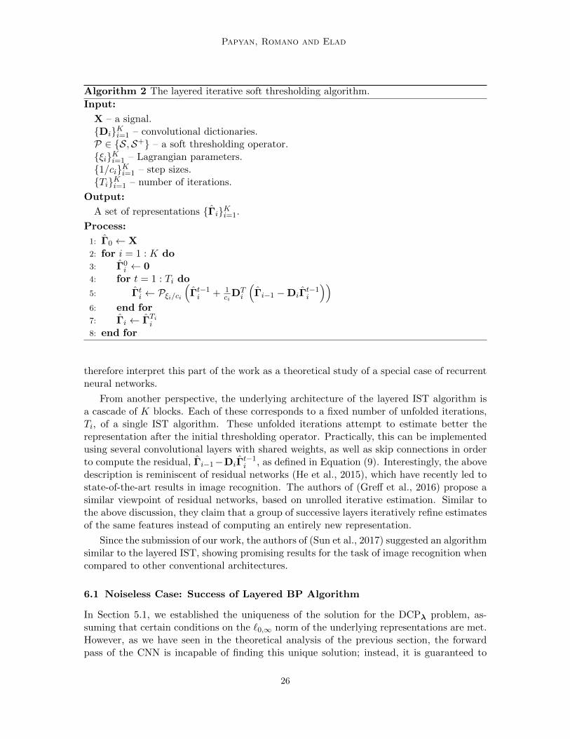
where Γti is the estimate of Γi at iteration t. The above can be interpreted as a simpleprojected gradient descent algorithm, where the constant ci is inversely proportional toits step size. As a result, if ci is chosen to be large enough7, the above algorithm isguaranteed to converge to its global minimum that is the solution of (8), as was shown in(Daubechies et al., 2004). The method obtained by gradually computing the set of sparserepresentations, ΓiKi=1, via the IST is summarized in Algorithm 2 and named layerediterative soft thresholding. Notice that this algorithm coincides with the simple layered softthresholding if it is run for a single iteration with ci = 1 and initialized with Γ0
i = 0. Thisimplies that the above algorithm is a natural extension to the forward pass of the CNN.Moreover, the above is similar to the approach taken in the work of deconvolutional networks(Zeiler et al., 2010), where the authors suggested to solve a sequence of BP problems acrossdifferent layers of abstraction.
With respect to the computational aspects of the IST algorithm, the work of (Gregorand LeCun, 2010) proposed the LISTA method, showing how the number of iterationsrequired by the IST to convergence can be reduced using neural networks. Later, (Giryeset al., 2016) proved the theoretical justification for this algorithm, and (Sprechmann et al.,2015) extended LISTA to other sparse and low-rank problems. Analogously, the work of(Xin et al., 2016) presented a generalization for the iterative hard thresholding (IHT), whichwas shown to be both theoretically and empirically superior to the original IHT.
The original motivation for the layered IST was its theoretical superiority over theforward pass algorithm – one that will be explored in detail in the next subsection. Yetmore can be said about this algorithm and the CNN architecture it induces. In (Gregor andLeCun, 2010) it was shown that the IST algorithm can be formulated as a simple recurrentneural network. As such, the same can be said regarding the layered IST algorithm proposedhere, with the exception that the induced recurrent network is much deeper. The reader can
7. The constant ci should satisfy ci > 0.5λmax
(DT
i Di
), where λmax
(DT
i Di
)is the maximal eigenvalue of
the gram matrix DTi Di (Combettes and Wajs, 2005).
25
Papyan, Romano and Elad
Algorithm 2 The layered iterative soft thresholding algorithm.
Input:
X – a signal.DiKi=1 – convolutional dictionaries.P ∈ S,S+ – a soft thresholding operator.ξiKi=1 – Lagrangian parameters.1/ciKi=1 – step sizes.TiKi=1 – number of iterations.
Output:
A set of representations ΓiKi=1.
Process:
1: Γ0 ← X2: for i = 1 : K do3: Γ0
i ← 04: for t = 1 : Ti do
5: Γti ← Pξi/ci(Γt−1i + 1
ciDTi
(Γi−1 −DiΓ
t−1i
))6: end for7: Γi ← ΓTii8: end for
therefore interpret this part of the work as a theoretical study of a special case of recurrentneural networks.
From another perspective, the underlying architecture of the layered IST algorithm isa cascade of K blocks. Each of these corresponds to a fixed number of unfolded iterations,Ti, of a single IST algorithm. These unfolded iterations attempt to estimate better therepresentation after the initial thresholding operator. Practically, this can be implementedusing several convolutional layers with shared weights, as well as skip connections in orderto compute the residual, Γi−1−DiΓ
t−1i , as defined in Equation (9). Interestingly, the above
description is reminiscent of residual networks (He et al., 2015), which have recently led tostate-of-the-art results in image recognition. The authors of (Greff et al., 2016) propose asimilar viewpoint of residual networks, based on unrolled iterative estimation. Similar tothe above discussion, they claim that a group of successive layers iteratively refine estimatesof the same features instead of computing an entirely new representation.
Since the submission of our work, the authors of (Sun et al., 2017) suggested an algorithmsimilar to the layered IST, showing promising results for the task of image recognition whencompared to other conventional architectures.
6.1 Noiseless Case: Success of Layered BP Algorithm
In Section 5.1, we established the uniqueness of the solution for the DCPλ problem, as-suming that certain conditions on the `0,∞ norm of the underlying representations are met.However, as we have seen in the theoretical analysis of the previous section, the forwardpass of the CNN is incapable of finding this unique solution; instead, it is guaranteed to
26
Convolutional Neural Networks Analyzed via Convolutional Sparse Coding
be close to it in terms of the `2,∞ norm. Herein, we address the question of whether thelayered BP algorithm can prevail in a task where the forward pass did not.
Theorem 11 (Layered BP recovery guarantee using the `0,∞ norm): Consider a signal X,
X = D1Γ1
Γ1 = D2Γ2
...
ΓK−1 = DKΓK ,
where DiKi=1 is a set of convolutional dictionaries and µ(Di)Ki=1 are their correspondingmutual coherences. Assuming that ∀ 1 ≤ i ≤ K
‖Γi‖S0,∞ <1
2
(1 +
1
µ(Di)
)then the layered BP algorithm is guaranteed to recover the set ΓiKi=1.
The proof for the above can be directly derived from the recovery condition of theBP using the `0,∞ norm, as presented in (Papyan et al., 2016a). The implications of thistheorem are that the layered BP algorithm can indeed recover the unique solution to theDCPλ problem.
6.2 Noisy Case: Stability of Layered BP Algorithm
Having established the guarantee for the success of the layered BP algorithm, we nowmove to its stability analysis. In particular, in a noisy scenario where obtaining the trueunderlying representations is impossible, does this algorithm remain stable? If so, howdo its guarantees compare to those of the layered thresholding algorithm? The followingtheorem, which we prove in Appendix F, aims to answer these questions.
Theorem 12 (Stability of the layered BP algorithm in the presence of noise): Suppose aclean signal X has a decomposition
X = D1Γ1
Γ1 = D2Γ2
...
ΓK−1 = DKΓK ,
and that it is contaminated with noise E to create the signal Y = X+E, such that ‖E‖P2,∞ ≤ε0. Let ΓiKi=1 be the set of solutions obtained by running the layered BP algorithm withparameters ξiKi=1. Assuming that ∀ 1 ≤ i ≤ K
a) ‖Γi‖S0,∞ ≤ 13
(1 + 1
µ(Di)
); and
b) ξi = 4εi−1,
27
Papyan, Romano and Elad
then
1. The support of the solution Γi is contained in that of Γi;
2. ‖Γi − Γi‖P2,∞ ≤ εi;
3. In particular, every entry of Γi greater in absolute value than εi√‖Γi‖P0,∞
is guaranteed
to be recovered; and
4. The solution Γi is the unique minimizer of the Lagrangian BP problem (Equation (8)),
where εi = ‖E‖P2,∞ 7.5i∏ij=1
√‖Γj‖P0,∞.
Several remarks are due at this point. The condition for the stability of the layeredthresholding algorithm, given by
‖Γi‖S0,∞ <1
2
(1 +
1
µ(Di)
|Γmini ||Γmaxi |
)− 1
µ(Di)
εi−1
|Γmaxi |
,
is expected to be more strict than that of the theorem presented above, which is
‖Γi‖S0,∞ <1
3
(1 +
1
µ(Di)
).
In the case of the layered BP algorithm, the bound on the `0,∞ norm of the underlyingsparse vectors does no longer depend on the ratio |Γmin
i |/|Γmaxi | – a term present in all
the theoretical results of the thresholding algorithm. Moreover, the `0,∞ norm becomesindependent of the local noise level of the previous layers, thus allowing more non-zeros perstripe.
In addition, similar to the stability analysis presented in Section 5.2, the above shows thegrowth (as a function of the depth) of the distance between the recovered representationsand the true ones.
7. A Closer Look at the Proposed Model
In this section, we revisit the assumptions of our model by imposing additional constraintson the dictionaries involved and showing their theoretical benefits. These additional as-sumptions originate from the current common practice of both CNN and sparsity.
7.1 When a Patch Becomes a Stripe
Throughout the analysis presented in this work, we have assumed that the representationsin the different layers, ΓiKi=1, are `0,∞-sparse. Herein, we study the propagation of the `0,∞norm throughout the layers of the network, showing how an assumption on the sparsity ofthe deepest representation ΓK reflects on that of the remaining layers. The exact connectionbetween the sparsities will be given in terms of a simple characterization of the dictionariesDiKi=1.
28
Convolutional Neural Networks Analyzed via Convolutional Sparse Coding
Consider the representation ΓK−1, given by
ΓK−1 = DKΓK ,
where ΓK is `0,∞-sparse. Following Figure 4, the i-th patch in ΓK−1 can be expressed as
PK−1,iΓK−1 = ΩK γK,i,
where ΩK is the stripe-dictionary of DK , the vector PK−1,iΓK−1 is the i-th patch in ΓK−1
and γK,i is its corresponding stripe. Recalling the definition of the ‖ · ‖P0,∞ norm (Definition6 in Section 5.3), we have that
‖ΓK−1‖P0,∞ = maxi‖ΩK γK,i‖0.
Consider the following definition.
Definition 13 Define the induced `0 pseudo-norm of a dictionary D, denoted by ‖D‖0, tobe the maximal number of non-zeros in any of its atoms8.
The multiplication ΩK γK,i can be seen as a linear combination of at most ‖γK,i‖0 atoms,each contributing no more than ‖ΩK‖0 non-zeros. As such
‖ΓK−1‖P0,∞ ≤ maxi‖ΩK‖0 ‖γK,i‖0.
Noticing that ‖ΩK‖0 = ‖DK‖0 (as can be seen in Figure 4), and using the definition of the‖ · ‖S0,∞ norm, we conclude that
‖ΓK−1‖P0,∞ ≤ ‖DK‖0 ‖ΓK‖S0,∞. (10)
In other words, given ‖ΓK‖S0,∞ and ‖DK‖0, we can bound the maximal number of non-zerosin a patch from ΓK−1.
The claims in Section 5 and 6 are given in terms of not only ‖ΓK−1‖P0,∞, but also‖ΓK−1‖S0,∞. According to Table 1, the length of a patch in ΓK−1 is nK−1mK−1, while thesize of a stripe is (2nK−2 − 1)mK−1. As such, we can fit (2nK−2 − 1)/nK−1 patches in astripe. Assume for simplicity that this ratio is equal to one. As a result, we obtain that apatch in the signal ΓK−1 extracted from the system
ΓK−1 = DKΓK ,
is also a stripe in the representation ΓK−1 when considering
ΓK−2 = DK−1ΓK−1,
hence the name of this subsection. Leveraging this assumption, we return to Equation (10)and obtain that
‖ΓK−1‖S0,∞ = ‖ΓK−1‖P0,∞ ≤ ‖DK‖0 ‖ΓK‖S0,∞.
8. According to the definition of the induced norm ‖D‖0 = maxv ‖Dv‖0 s.t. ‖v‖0 = 1. Since ‖v‖0 = 1,the multiplication Dv is simply equal to one of the atoms in D times a scalar, and ‖Dv‖0 counts thenumber of non-zeros in this atom. As a result, ‖D‖0 is equal to the maximal number of non-zeros in anyatom from D.
29
Papyan, Romano and Elad
Using the same rationale for the remaining layers, and assuming that once again the patchesbecome stripes, we conclude that
‖Γi‖S0,∞ = ‖Γi‖P0,∞ ≤ ‖ΓK‖S0,∞K∏
j=i+1
‖Dj‖0. (11)
We note that our assumption here of having sparse dictionaries is reasonable, since at thetraining stage of the CNN an `1 penalty is often imposed on the filters as a regularization,promoting their sparsity. The conclusion thus is that the `0,∞ norm is expected to decreaseas a function of the depth of the representation. This aligns with the intuition that thehigher the depth, the more abstraction one obtains in the filters, and thus the less non-zerosare required to represent the data. Taking this to the extreme, if every input signal couldbe represented via a single coefficient at the deepest layer, we would obtain that its `0,∞norm is equal to one.
7.2 On the Role of the Spatial-Stride
A common step among practitioners of CNN (Krizhevsky et al., 2012; Simonyan and Zisser-man, 2014; He et al., 2015) is to convolve the input to each layer with a set of filters, skippinga fixed number of spatial locations in a regular pattern. One of the primary motivationsfor this is to reduce the dimensions of the kernel maps throughout the layers, leading tocomputational benefits. In this subsection we unveil some theoretical benefits of thiscommon practice, which we coin spatial-stride.
Following Figure 5, recall that Di is a stride convolutional dictionary that skips mi−1
shifts at a time, which correspond to the number of channels in Γi−1. Translating thespatial-stride to our language, the above mentioned works do not consider all spatial shiftsof the filters in Di. Instead, a stride of mi−1si−1 is employed, where mi−1 correspondsto the channel-stride, while si−1 is due to the spatial-stride. The addition of the latterimplies that instead of assuming that the i-th sparse vector satisfies Γi−1 = DiΓi, we havethat Qi−1Γi−1 = DiQ
Ti QiΓi. We denote QT
i ∈ RNmi×Nmi/si−1 as a columns’ selectionoperator that chooses the atoms from Di that align with the spatial-stride. The coefficientscorresponding to these atoms are extracted from Γi (resulting in its subsampled version) viathe Qi matrix. In light of the above discussion, we modify the DCPλ problem, as definedin Definition 1, into the following
find ΓiKi=1 s.t. X = D1QT1 Q1Γ1, ‖Q1Γ1‖S0,∞ ≤ λ1
Q1Γ1 = D2QT2 Q2Γ2, ‖Q2Γ2‖S0,∞ ≤ λ2
......
QK−1ΓK−1 = DKQTKQKΓK , ‖QKΓK‖S0,∞ ≤ λK .
Note that while the original ‖Γi‖S0,∞ is equal to the maximal number of non-zeros in a stripeof length (2ni−1 − 1)mi in Γi, the term ‖QiΓi‖S0,∞ counts the same quantity but for stripesof length (2 dni−1/si−1e − 1)mi in QiΓi.
According to the study in Section 5 and 6, the theoretical advantage of the spatial-strideis twofold. First, consider the mutual coherence of the stride convolutional dictionary Di.
30
Convolutional Neural Networks Analyzed via Convolutional Sparse Coding
Due to the locality of the filters and their restriction to certain spatial shifts, the mutualcoherence of DiQ
Ti is expected to be lower than that of Di, thus leading to more non-zeros
allowed per stripe. Second, the length of a stripe in QiΓi is equal to (2 dni−1/si−1e− 1)mi,while that of Γi is (2ni−1− 1)mi. As such, our analysis allows a larger number of non-zerosper a smaller-sized stripe. From another perspective, notice that imposing a spatial-strideon the dictionary Di is equivalent to forcing a portion of the entries in Γi to be zero. Assuch, the spatial-stride encourages sparser solutions.
8. Experiments: The Generator Behind the CNN
Consider the following question: can we synthesize signals obeying the ML-CSC model?Throughout this work we have posited that the answer to this question is positive; we haveassumed the existence of a set of signals X, which satisfy ∀i Γi = Di+1Γi+1 where ΓiKi=1
are all `0,∞ bounded. However, a natural question arises as to whether we can give a simpleexample of set of dictionaries DiKi=1 and their corresponding signals X that indeed satisfyour model assumptions.
A naıve attempt would be to choose an arbitrary set of dictionaries, DiKi=1, and arandom deepest representation, ΓK , and compute the remaining sparse vectors (and thesignal itself) using the set of relations Γi = Di+1Γi+1. However, without further restrictions,this would lead to a set of representations ΓiKi=1 with growing `0,∞ norm as we propagatetowards Γ0. A somewhat better approach would be to impose sparsity on the dictionariesinvolved, as suggested in Section 7.1, thus leading to sparser representations. However,besides the obvious drawback of forcing a limiting structure on the dictionaries, as can beseen in Equation (11), in the worst case this would also lead to growth in the density of therepresentations, even if it is more controlled. The spatial-stride – at first glance unrelatedto this discussion – is another solution that addresses the same problem. In particular, inSection 7.2 this idea was shown to encourage sparser vectors by forcing zeros in a regularpattern in the set of representations ΓiKi=1.
In this section we combine the above notions in order to achieve our goal – generate a setof signals that will satisfy the ML-CSC assumptions. These will then serve as a playgroundfor several experiments, which will compare both theoretically and practically the differentpursuits presented in this paper.
8.1 Designing the Dictionaries
We commence by describing the design of the dictionaries, and in the next subsectioncontinue to the actual generation of the signals. In our experiments, the signal is onedimensional and therefore m0 = 1. Moreover, for simplicity, the dictionary in every layercontains a single atom with its shifts and thus mi = 1 ∀1 ≤ i ≤ K. We should note thatthe choice of a single atom simplifies the involved pursuit problem, but as we will see, evenin such a case the suggested layered pursuits (including the forward pass) may fail. This isbecause the mutual coherence and the amount of non-zeros are still non-trivial.
In the first layer we choose this filter to be the analytically defined discrete MeyerWavelet of length n0 = 29. In order to obtain sparser representations and improve thecoherence of the global dictionary D1, we employ a stride of s0 = 6, resulting in µ(D1) =2.44 × 10⁻⁴. As a consequence of our choice of D1, the signals resulting from our model
31
Papyan, Romano and Elad
are a superposition of shifted versions of discrete Meyer Wavelets, multiplied by differentcoefficients.
Recall that in the context of the layered thresholding algorithm, our theoretical studyhas shown that the stability of the pursuit depends on the ratio |Γmin
i |/|Γmaxi |. As such, in
addition to requiring µ(Di) to be small, we would also like the ratio |Γmini |/|Γmax
i | to be asclose as possible to one. Since the sparse vectors satisfy Γi = Di+1Γi+1 ∀1 ≤ i ≤ K−1, onecan control this ratio by forcing the entries in the dictionaries DiKi=2 to be9 discrete10.Following this observation, and motivated by the benefits of a sparse dictionary, we generatea filter of length 20 with 7 non-zero entries belonging to the set −8,−7, ..., 7, 8 (these arethe entries before the atom is normalized to a unit `2 norm). In practice, this is done bysampling random vectors satisfying these constraints and choosing one resulting in a goodmutual coherence. For simplicity, all DiKi=2 are created from the very same local atom,i.e. ni = 20 ∀1 ≤ i ≤ K − 1. Moreover, in all the dictionaries this atom is shifted by astride of si = 6, leading to µ(Di) = 4.33 × 10⁻³. Note that in the above description thespecific number of layers K was purposely omitted, as this number will vary in the followingexperiments.
8.2 Noiseless Experiments
We now move to the task of sampling a signal when the number of layers is K = 3. First,we draw a random Γ3 of length 100 with an `0 norm in the range [20, 66] and set each non-zero coefficient in it to ±1, with equal probability. Given the dictionaries and the sampledsparse vector Γ3, we then compute the representations Γ2, Γ1 and the signal X, which areof length 600, 3, 600 and N = 21, 600, respectively. The obtained sparse vectors satisfy‖Γ1‖S0,∞ = 8, 5 ≤ ‖Γ2‖S0,∞ ≤ 6 and 3 ≤ ‖Γ3‖S0,∞ ≤ 7.
Given the signals, we attempt to retrieve their underlying representations using thelayered pursuits presented in this work. Recall that our analysis in Section 5 and 6 indicatesthat the layered hard thresholding is superior to its soft counterpart, which is equivalentto the forward pass, and that the layered BP is even better than both of these algorithms.We now turn to asserting this claim empirically. While doing so, we aim to study thegap between the theoretical guarantees presented throughout our paper and the empiricalperformance obtained in practice.
For every signal X (termed realization below), we employ the layered hard thresholdingalgorithm. The thresholds are set to be the ones presented in Theorem 8, since the `0,∞norms of the representations of each X satisfy the assumptions of this theorem. Given theestimated sparse vectors Γi3i=1, we then compute the errors ‖Γi − Γi‖P2,∞ and comparethese to the theoretical bounds. While doing so, we also verify that the correct supportis indeed retrieved, as our theorem guarantees. Next, the same process is repeated for the
9. Note that we do not force the entries in D1 to be discrete since X = D1Γ1 and the ratio of the entriesin X is of no significance to the success of the layered thresholding algorithms.
10. In our experiments, the non-zero entries in the deepest representation ΓK are chosen to be ±1. Assuch, the sparse vector ΓK−1 = DKΓK is a superposition of filters (or their negative) taken from thedictionary DK . If the entries in DK are non-discrete then the summation of two filters can result inextremely small values in ΓK−1, which in turn would lead to a very small |Γmin
K−1| and a bad ratio. Onthe other hand, if the atoms are chosen to be discrete, this would not happen since the entries wouldsimply cancel each other.
32
Convolutional Neural Networks Analyzed via Convolutional Sparse Coding
layered soft thresholding algorithm, with the exception that the thresholds and the boundon the distance are computed according to Theorem 10. We note that the assumptions ofthis hold as well for every signal X. The results for both algorithms are depicted in Figure
6 in terms of the local signal to noise ratio (SNR), defined as 20 log 10( ‖Γi‖P2,∞‖Γi−Γi‖P2,∞
). Due to
the locality of the analysis, we choose to deviate from the classical definition of the (global)
SNR, given by 20 log 10(‖Γi‖2‖Γi−Γi‖2
).
Several remarks are due here. First and foremost, the theoretical bounds indeed hold,since the blue points are above their corresponding green ones and the correct supports arealways recovered. Second, our analysis predicts that the distance between the estimatedsparse representation, Γi, and the true ones, Γi, should increase with the layer. This isevident by the decrease in the values of the green points with the layers. The empiricalresults presented here (blue dots) corroborate this prognosis, as the error in both algorithmsis lowest in the first layer and highest in the last11. Third, our analysis suggests that thelayered hard thresholding algorithm should be superior to its soft counterpart. Once again,this can be deduced from the figure by comparing the values of the green points in both ofthe algorithms. The empirical results presented in Figure 6 confirm this behavior, as canbe clearly seen by comparing the errors (blue points) obtained by both algorithms in thei-th layer. One should note that the performance gap exhibited here is due to the constantβi being subtracted from every entry in the soft thresholding algorithm.
The implications of the above discussion might be troubling in the context of CNN, aswhat this experiment shows is a deterioration of the empirical SNR throughout the layersof the network. Is this truly the behavior of CNN? Recall that in practice the biases of thedifferent layers (thresholds) are learned in order to achieve the best possible performance insolving a certain task. As such, it might be possible that the decline in SNR presented hereis alleviated when better thresholds are employed in lieu of the theoretical ones used thusfar. We demonstrate this by running the layered soft thresholding algorithm with an oracleparameter, chosen to be the minimal threshold that leads to ‖Γi‖0 non-zeros being chosenin the estimated sparse representation Γi. The results for this are presented in Figure 6and colored in red. Indeed, we observe that this better choice of parameters improvesthe empirical performance of the layered soft thresholding algorithm and leads to a slowerdecline in SNR. Still, the performance of the layered soft thresholding is inferior to that ofits hard variant12, as can be seen by comparing the red points with the blue ones in thesubplots below.
Next, we proceed our experiments by running the layered BP algorithm, as defined inSection 6, on the same set of signals. Recall that one of the prime motivations for proposingthis algorithm was its ability to retrieve the exact underlying representations, as justifiedtheoretically in Theorem 11. In our experiments, we validate this claim by checking that itsconditions hold for each signal and that the underlying representations are indeed retrieved.We omit showing a plot for this and comparing it to the layered thresholding algorithmssince the errors obtained are simply zeros.
11. Interestingly, the error in the layered hard thresholding algorithm is approximately equal in the secondand third layers.
12. Note that in the layered hard thresholding, as long as the correct support is chosen, the threshold doesnot affect the error and as such the oracle version for it is meaningless.
33
Papyan, Romano and Elad
100 200 300 40010
20
30
40
50
60
70
SNR
[dB]
Layer 1
100 200 300 40010
20
30
40
50
60
70
Realization
Layered Soft Thresholding
Layer 2
100 200 300 40010
20
30
40
50
60
70
Layer 3
100 200 300 40010
20
30
40
50
60
70
SNR
[dB]
Layer 1
100 200 300 40010
20
30
40
50
60
70
Realization
Layered Hard Thresholding
Layer 2
100 200 300 40010
20
30
40
50
60
70
Layer 3
Figure 6: Comparison between the performance of the layered thresholding algorithms in anoiseless setting. All the signals presented here satisfy the assumptions of Theorem 8 and10 and indeed the correct support of all the representations are recovered. The horizontalaxis plots the realization number, while the vertical axis shows the SNR (the higher thebetter). Blue: layered thresholding algorithm with the theoretically justifiable thresholds.Green: the theoretical bound on the error. Red: layered soft thresholding algorithm withoracle thresholds. Note that the points are sorted according to the theoretical bound.
34
Convolutional Neural Networks Analyzed via Convolutional Sparse Coding
8.3 Noisy Experiments
Having established the stability of our proposed algorithms in a perfect scenario, whereε0 = 0, we now turn to a noisy setting. Naturally, the estimation task becomes noweven more challenging – not only does the SNR drop with each layer, as demonstratedpreviously, but also the input SNR is no longer infinity. In order to facilitate the success ofour algorithms, in this section we demonstrate the empirical performance and theoreticalbounds on K = 2 layers and a small noise level.
Similar to the previous subsection, we begin by sampling a signal X. To this end, wedraw a random Γ2 of length 100 where 20 ≤ ‖Γ2‖0 ≤ 66. Each non-zero coefficient in it isthen set to ±1, with equal probability. Given the dictionaries and the sampled sparse vectorΓ2, we then compute the representation Γ1 and the signal X, which are of length 600 and3, 600, respectively. The `0,∞ norm of the obtained sparse vectors satisfies 7 ≤ ‖Γ1‖S0,∞ ≤ 8and 3 ≤ ‖Γ2‖S0,∞ ≤ 7.
Next, we contaminate each signal X with a zero-mean white additive Gaussian noise E,creating a signal Y = X + E. The average SNR of the obtained noisy signals is 68.53 dB.These are then fed into the layered pursuits, resulting in a set of estimated sparse repre-sentations, Γi. We note that the `0,∞ norms of the representations of each X satisfy theassumptions of Theorem 8, 10 and 12. As such, the parameters for every algorithm arechosen according to our theoretical study. For each estimated representation we computethe error ‖Γi − Γi‖P2,∞ and its corresponding theoretical bound obtained from the afore-mentioned theorems. Since the underlying representations satisfy the assumptions of thestability theorem for the layered thresholding algorithms, for each signal we verify thatindeed the correct support is found. As for the layered BP, our stability analysis guaranteesthat the support retrieved should be contained in the true one and coefficients that are largeenough in Γi should be retrieved. In practice, the layered BP always finds the full support.
We present the obtained results in terms of the local SNR in Figure 7, showing the sta-bility of the different algorithms that is in accordance with our theoretical bounds. Similarto the noiseless experiment, we observe that for all the algorithms the error increases boththeoretically (green points) and empirically (blue points) with the layer depth. As previ-ously discussed, a performance gap exists between the soft and hard layered thresholdingalgorithms. To mitigate this, we run the layered soft thresholding with an oracle parameterand compare the obtained errors (red points) to those of the other algorithms. The results,depicted in the same figure, show a clear improvement in the performance.
Interestingly, although theoretically superior, the layered BP leads to similar perfor-mance to that of the layered soft thresholding and worse performance than that of the lay-ered hard thresholding (when comparing the blue points). We attribute this phenomenonto the suboptimal choice of the parameter ξi, which was chosen thus far according to ourtheoretical analysis. To validate this suspicion, we run the layered BP with hand-picked ξiand plot the obtained SNR in red in Figure 7. Not only are the correct supports retrievedfor all the signals, but we can also see a clear improvement in terms of the SNR. In the firstlayer, the layered BP outperforms the layered soft thresholding and leads to similar resultsto those of the layered hard thresholding, while in the second, the layered BP significantlyoutperforms both of the other pursuit algorithms.
35
Papyan, Romano and Elad
50 100 150 200 250 300 35020
30
40
50
60
70
Realization
SNR
[dB]
Layered Soft Thresholding
Layer 1
50 100 150 200 250 300 35020
30
40
50
60
70
Layer 2
50 100 150 200 250 300 35020
30
40
50
60
70
Realization
SNR
[dB]
Layered Hard Thresholding
Layer 1
50 100 150 200 250 300 35020
30
40
50
60
70
Layer 2
50 100 150 200 250 300 35020
30
40
50
60
70
Realization
SNR
[dB]
Layered BP
Layer 1
50 100 150 200 250 300 35020
30
40
50
60
70
Layer 2
Figure 7: Comparison between the performance of the layered pursuit algorithms in a noisysetting. All the signals presented here satisfy the assumptions of Theorem 8, 10 and 12and the correct support of all the representations are indeed recovered. The horizontal axisplots the realization number, while the vertical axis shows the SNR (the higher the better).Blue: layered pursuits with the theoretically justifiable thresholds. Green: the theoreticalbound on the error. Red: layered soft thresholding with oracle thresholds and layered BPwith hand-picked parameters. Note that the points are sorted according to the theoreticalbound.
36
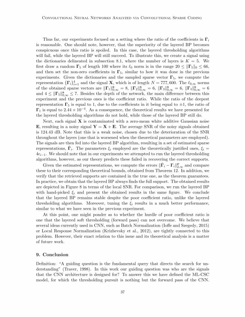
Convolutional Neural Networks Analyzed via Convolutional Sparse Coding
Thus far, our experiments focused on a setting where the ratio of the coefficients in Γiis reasonable. One should note, however, that the superiority of the layered BP becomesconspicuous once this ratio is spoiled. In this case, the layered thresholding algorithmswill fail, while the layered BP will still succeed. To illustrate this, we create a signal usingthe dictionaries delineated in subsection 8.1, where the number of layers is K = 5. Wefirst draw a random Γ5 of length 100 where its `0 norm is in the range 20 ≤ ‖Γ5‖0 ≤ 66,and then set the non-zero coefficients in Γ5, similar to how it was done in the previousexperiments. Given the dictionaries and the sampled sparse vector Γ5, we compute therepresentation Γi4i=1 and the signal X, which is of length N = 777, 600. The `0,∞ normsof the obtained sparse vectors are ‖Γ1‖S0,∞ = 8, ‖Γ2‖S0,∞ = 6, ‖Γ3‖S0,∞ = 6, ‖Γ4‖S0,∞ = 6and 4 ≤ ‖Γ5‖S0,∞ ≤ 7. Besides the depth of the network, the main difference between thisexperiment and the previous ones is the coefficient ratio. While the ratio of the deepestrepresentation Γ5 is equal to 1, due to the coefficients in it being equal to ±1, the ratio ofΓ1 is equal to 2.44× 10⁻⁴. As a consequence, the theoretical results we have presented forthe layered thresholding algorithms do not hold, while those of the layered BP still do.
Next, each signal X is contaminated with a zero-mean white additive Gaussian noiseE, resulting in a noisy signal Y = X + E. The average SNR of the noisy signals obtainedis 124.43 dB. Note that this is a weak noise, chosen due to the deterioration of the SNRthroughout the layers (one that is worsened when the theoretical parameters are employed).The signals are then fed into the layered BP algorithm, resulting in a set of estimated sparserepresentations, Γi. The parameters ξi employed are the theoretically justified ones, ξi =4εi−1. We should note that in our experiments we attempted to run the layered thresholdingalgorithms, however, as our theory predicts these failed in recovering the correct supports.
Given the estimated representations, we compute the errors ‖Γi − Γi‖P2,∞ and comparethese to their corresponding theoretical bounds, obtained from Theorem 12. In addition, weverify that the retrieved supports are contained in the true one, as the theorem guarantees.In practice, we obtain that the layered BP always finds the full support. The obtained resultsare depicted in Figure 8 in terms of the local SNR. For comparison, we run the layered BPwith hand-picked ξi and present the obtained results in the same figure. We concludethat the layered BP remains stable despite the poor coefficient ratio, unlike the layeredthresholding algorithms. Moreover, tuning the ξi results in a much better performance,similar to what we have seen in the previous experiment.
At this point, one might ponder as to whether the hurdle of poor coefficient ratio isone that the layered soft thresholding (forward pass) can not overcome. We believe thatseveral ideas currently used in CNN, such as Batch Normalization (Ioffe and Szegedy, 2015)or Local Response Normalization (Krizhevsky et al., 2012), are tightly connected to thisproblem. However, their exact relation to this issue and its theoretical analysis is a matterof future work.
9. Conclusion
Definition: “A guiding question is the fundamental query that directs the search for un-derstanding” (Traver, 1998). In this work our guiding question was who are the signalsthat the CNN architecture is designed for? To answer this we have defined the ML-CSCmodel, for which the thresholding pursuit is nothing but the forward pass of the CNN.
37
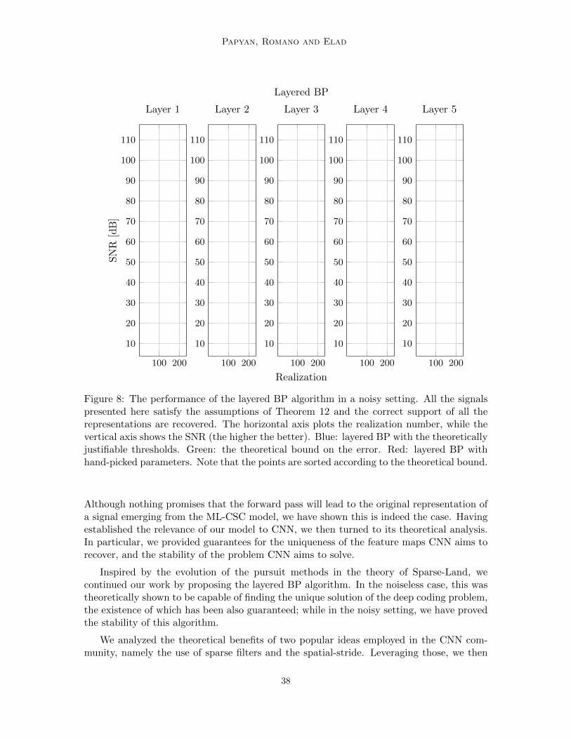
Papyan, Romano and Elad
100 200
10
20
30
40
50
60
70
80
90
100
110
SNR
[dB]
Layer 1
100 200
10
20
30
40
50
60
70
80
90
100
110
Layer 2
100 200
10
20
30
40
50
60
70
80
90
100
110
Realization
Layered BP
Layer 3
100 200
10
20
30
40
50
60
70
80
90
100
110
Layer 4
100 200
10
20
30
40
50
60
70
80
90
100
110
Layer 5
Figure 8: The performance of the layered BP algorithm in a noisy setting. All the signalspresented here satisfy the assumptions of Theorem 12 and the correct support of all therepresentations are recovered. The horizontal axis plots the realization number, while thevertical axis shows the SNR (the higher the better). Blue: layered BP with the theoreticallyjustifiable thresholds. Green: the theoretical bound on the error. Red: layered BP withhand-picked parameters. Note that the points are sorted according to the theoretical bound.
Although nothing promises that the forward pass will lead to the original representation ofa signal emerging from the ML-CSC model, we have shown this is indeed the case. Havingestablished the relevance of our model to CNN, we then turned to its theoretical analysis.In particular, we provided guarantees for the uniqueness of the feature maps CNN aims torecover, and the stability of the problem CNN aims to solve.
Inspired by the evolution of the pursuit methods in the theory of Sparse-Land, wecontinued our work by proposing the layered BP algorithm. In the noiseless case, this wastheoretically shown to be capable of finding the unique solution of the deep coding problem,the existence of which has been also guaranteed; while in the noisy setting, we have provedthe stability of this algorithm.
We analyzed the theoretical benefits of two popular ideas employed in the CNN com-munity, namely the use of sparse filters and the spatial-stride. Leveraging those, we then
38
Convolutional Neural Networks Analyzed via Convolutional Sparse Coding
generated signals satisfying the ML-CSC assumptions and demonstrated the performanceof the pursuits presented throughout this work.
We conclude this work by presenting our ongoing research directions:
1. Through this paper we have assumed the worst – an adversary noise. Can our theo-retical analysis be extended to a setting where the noise is random?
2. Thus far in tackling the deep coding problem, we have restricted ourself to existingmethods, such as the forward pass of the CNN or deconvolutional networks (Zeileret al., 2010). Can we suggest better approximations for the solution of this problem?
3. What is the role of common tricks currently employed in CNN in the context ofthe ML-CSC model? These include but are not limited to, Batch Normalization(Ioffe and Szegedy, 2015), Local Response Normalization (Krizhevsky et al., 2012),Dropout (Srivastava et al., 2014) and Pooling (LeCun et al., 1990; Krizhevsky et al.,2012; Simonyan and Zisserman, 2014).
Acknowledgments
The research leading to these results has received funding in part from the European Re-search Council under EU’s 7th Framework Program, ERC under Grant 320649, and in partby Israel Science Foundation (ISF) grant no. 1770/14. The authors would like to thankJeremias Sulam for the inspiring discussions and creative advice.
Appendix A.Uniqueness via the Mutual Coherence (Proof of Theorem 4)
Proof In (Papyan et al., 2016a) a solution Γ to the P0,∞ problem, as defined in Equation
(6), was shown to be unique assuming that ‖Γ‖S0,∞ < 12
(1 + 1
µ(D)
). In other words, if the
true representation is sparse enough in the `0,∞ sense, no other solution is possible. Herein,we leverage this claim in order to prove the uniqueness of the DCPλ problem.
Let ΓiKi=1 be a set of representations of the signal X, obtained by solving the DCPλ
problem. According to our assumptions, ‖Γ1‖S0,∞ < 12
(1 + 1
µ(D1)
). Moreover, since the set
ΓiKi=1 is a solution of the DCPλ problem, we also have that ‖Γ1‖S0,∞ ≤ λ1 <12
(1 + 1
µ(D1)
).
As such, in light of the aforementioned uniqueness theorem, both representations are equal.Once we have concluded that Γ1 = Γ1, we would also like to show that the representa-
tions Γ2 and Γ2 are identical. Similarly, the assumptions ‖Γ2‖S0,∞ < 12
(1 + 1
µ(Di)
)and
‖Γ2‖S0,∞ ≤ λ2 < 12
(1 + 1
µ(D2)
)guarantee that Γ2 = Γ2. The same set of steps can be
applied for all 1 ≤ i ≤ K, leading to the fact that both sets of representations are identical.
39
Papyan, Romano and Elad
Appendix B.Global Stability of the DCPE
λ Problem (Proof of Theorem 5)
Proof In (Papyan et al., 2016b), for a signal Y = X + E = D1Γ1 + E, it was shown thatif the following hold:
1. ‖Γ1‖S0,∞ ≤ λ1 <12
(1 + 1
µ(D1)
)and ‖E‖2 = ‖Y −D1Γ1‖2,
2. ‖Γ1‖S0,∞ ≤ λ1 <12
(1 + 1
µ(D1)
)and ‖Y −D1Γ1‖2 ≤ ‖E‖2,
then
‖Γ1 − Γ1‖22 ≤4‖E‖22
1− (2λ1 − 1)µ(D1).
In item 2 we have used the fact that the solution for the DCPEλ problem, Γ1, must satisfy
‖Y−D1Γ1‖2 ≤ ‖E‖2 and ‖Γ1‖S0,∞ ≤ λ1. Notice that the true solution satisfies Γ1 = D2Γ2
and also the solution of DCPEλ satisfies Γ1 = D2Γ2. As such,
‖D2Γ2 −D2Γ2‖22 = ‖Γ1 − Γ1‖22 ≤4‖E‖22
1− (2λ1 − 1)µ(D1). (12)
Using the definition of SRIP from (Papyan et al., 2016b) and the fact that
‖Γ2 − Γ2‖S0,∞ ≤ 2λ2
we have
(1− δ2λ2) ‖Γ2 − Γ2‖22 ≤ ‖D2Γ2 −D2Γ2‖22,
where δ2λ2 is the SRIP constant of D2 for an `0,∞ norm equal to 2λ2. Bounding the SRIPusing the mutual coherence, as was done in (Papyan et al., 2016b), the above results in
(1− (2λ2 − 1)µ(D2)) ‖Γ2 − Γ2‖22 ≤ (1− δ2λ2) ‖Γ2 − Γ2‖22≤‖D2Γ2 −D2Γ2‖22.
Combining this together with Equation (12), we obtain
‖Γ2 − Γ2‖22 ≤4‖E‖22
(1− (2λ1 − 1)µ(D1)) (1− (2λ2 − 1)µ(D2)).
Repeating the above set of steps for the deeper layers, we conclude that
∀ 1 ≤ i ≤ K ‖Γi − Γi‖22 ≤ 4‖E‖22i∏
j=1
1
1− (2λj − 1)µ(Dj),
as claimed.
40
Convolutional Neural Networks Analyzed via Convolutional Sparse Coding
Appendix C.Stable Recovery of Hard Thresholding in the Presence of Noise (Proof ofLemma 7)
Proof Denote by T1 the support of Γ1. Denote further the i-th atom from D1 by d1,i.The success of the hard thresholding algorithm with threshold β1 in recovering the correctsupport is guaranteed if the following holds
mini∈T1
∣∣dT1,iY∣∣ > β1 > maxj /∈T1
∣∣dT1,jY∣∣ .Using the same set of steps as those used in proving Theorem 4 in (Papyan et al., 2016b),we can lower bound the left-hand-side by
mini∈T1
∣∣dT1,iY∣∣ ≥ |Γmin1 | − (‖Γ1‖S0,∞ − 1)µ(D1)|Γmax
1 | − ε0
and upper bound the right-hand-side via
‖Γ1‖S0,∞µ(D1)|Γmax1 |+ ε0 ≥ max
j /∈T1
∣∣dT1,jY∣∣ .Next, by requiring
mini∈T1
∣∣dT1,iY∣∣ ≥|Γmin1 | − (‖Γ1‖S0,∞ − 1)µ(D1)|Γmax
1 | − ε0 (13)
> β1
>‖Γ1‖S0,∞µ(D1)|Γmax1 |+ ε0
≥maxj /∈T1
∣∣dT1,jY∣∣ ,we ensure the success of the thresholding algorithm. This condition can be equally writtenas
‖Γ1‖S0,∞ <1
2
(1 +
1
µ(D1)
|Γmin1 ||Γmax
1 |
)− 1
µ(D1)
ε0|Γmax
1 |.
Equation (13) also implies that the threshold β1 that should be employed must satisfy
|Γmin1 | − (‖Γ1‖S0,∞ − 1)µ(D1)|Γmax
1 | − ε0 > β1 > ‖Γ1‖S0,∞µ(D1)|Γmax1 |+ ε0. (14)
Thus far, we have considered the successful recovery of the support of Γ1. Next, assum-ing this correct support was recovered, we shall dwell on the deviation of the thresholdingresult, Γ1, from the true Γ1. Denote by Γ1,T1 and Γ1,T1 the vectors Γ1 and Γ1 restricted tothe support T1, respectively. We have that
‖Γ1 − Γ1‖∞ = ‖Γ1,T1 − Γ1,T1‖∞
=∥∥∥(DT
1,T1D1,T1)−1
DT1,T1X−DT
1,T1Y∥∥∥∞
=∥∥∥((DT
1,T1D1,T1)−1
DT1,T1 −DT
1,T1
)X−DT
1,T1(Y −X)∥∥∥∞,
41
Papyan, Romano and Elad
where the Gram DT1,T1D1,T1 is invertible according to Lemma 1 in (Papyan et al., 2016a).
Using the triangle inequality of the `∞ norm and the relation X = D1,T1Γ1,T1 , we obtain
‖Γ1 − Γ1‖∞ ≤∥∥∥((DT
1,T1D1,T1)−1
DT1,T1 −DT
1,T1
)D1,T1Γ1,T1
∥∥∥∞
+∥∥∥DT
1,T1(Y −X)∥∥∥∞
=∥∥(I−DT
1,T1D1,T1)Γ1,T1
∥∥∞ +
∥∥DT1,T1(Y −X)
∥∥∞ ,
where I is an identity matrix. Relying on the definition of the induced `∞ norm, the aboveis equal to
‖Γ1 − Γ1‖∞ ≤∥∥I−DT
1,T1D1,T1∥∥∞ · ‖Γ1,T1‖∞ +
∥∥DT1,T1(Y −X)
∥∥∞ . (15)
In what follows, we shall upper bound both of the expressions in the right hand side of theinequality.
Beginning with the first term in the above inequality,∥∥∥I−DT
1,T1D1,T1
∥∥∥∞
, recall that the
induced infinity norm of a matrix is equal to its maximum absolute row sum. The diagonalentries of I − DT
1,T1D1,T1 are equal to zero, due to the normalization of the atoms, whilethe off diagonal entries can be bounded by relying on the locality of the atoms and thedefinition of the `0,∞ norm. As such, each row has at most ‖Γ1‖S0,∞ − 1 non-zeros, whereeach is bounded by µ(D1) based on the definition of the mutual coherence. We concludethat the maximum absolute row sum can be bounded by
‖DT1,T1D1,T1 − I‖∞ ≤ (‖Γ1‖S0,∞ − 1)µ(D1). (16)
Next, moving to the second expression, define R1,i ∈ Rn0×N to be the operator that extractsa filter of length n0 from d1,i. Consequently, the operator RT
1,i pads a local filter of lengthn0 with zeros, resulting in a global atom of length N . Notice that, due to the locality ofthe atoms RT
1,iR1,id1,i = d1,i. Using this together with the Cauchy-Schwarz inequality, thenormalization of the atoms, and the local bound on the error ‖Y −X‖P2,∞ ≤ ε0, we havethat ∥∥DT
1,T1(Y −X)∥∥∞ = max
i∈T1
∣∣dT1,i(Y −X)∣∣ (17)
= maxi∈T1
∣∣∣(R1,id1,i)T R1,i(Y −X)
∣∣∣≤ max
i∈T1‖R1,id1,i‖2 · ‖R1,i(Y −X)‖2
≤ 1 · ‖Y −X‖P2,∞≤ ε0.
In the second to last inequality we have used Definition 6, denoting the maximal `2 normof a patch extracted from Y −X by ‖Y −X‖P2,∞. Plugging (16) and (17) into Equation(15), and using the fact that ‖Γ1,T1‖∞ = |Γmax
1 |, we obtain that
‖Γ1 − Γ1‖∞ ≤ (‖Γ1‖S0,∞ − 1)µ(D1)|Γmax1 |+ ε0. (18)
In the remainder of this proof we will localize the above bound into one that is posed interms of patch-errors. Note that ‖Γ1 − Γ1‖P2,∞ is equal to the maximal energy of an n1m1-dimensional patch taken from it, where the i-th patch can be extracted using the operator
42
Convolutional Neural Networks Analyzed via Convolutional Sparse Coding
P1,i. Relying on this and the relation ‖V‖2 ≤√‖V‖0 ‖V‖∞, we have that
‖Γ1 − Γ1‖P2,∞ = maxi
∥∥∥P1,i
(Γ1 − Γ1
)∥∥∥2
≤ maxi
√∥∥∥P1,i
(Γ1 − Γ1
)∥∥∥0
∥∥∥P1,i
(Γ1 − Γ1
)∥∥∥∞.
Recalling that, based on Definition 6, ‖Γ1 − Γ1‖P0,∞ denotes the maximal number of non-zeros in a patch of length n1m1 extracted from this vector, we obtain that
‖Γ1 − Γ1‖P2,∞ ≤√‖Γ1 − Γ1‖P0,∞ ‖Γ1 − Γ1‖∞
≤√‖Γ1‖P0,∞ ‖Γ1 − Γ1‖∞.
In the last inequality we have used the success of the first stage in recovering the correctsupport, resulting in ‖Γ1 − Γ1‖P0,∞ ≤ ‖Γ1‖P0,∞. Plugging inequality (18) into the aboveequation, we conclude that
‖Γ1 − Γ1‖P2,∞ ≤√‖Γ1‖P0,∞
(ε0 + µ(D1)
(‖Γ1‖S0,∞ − 1
)|Γmax
1 |),
as claimed.
Appendix D.Stability of the Layered Hard Thresholding in the Presence of Noise(Proof of Theorem 8)
Proof The stability of the first stage of the layered hard thresholding algorithm is obtainedfrom Lemma 7. Denoting by ∆1 = Γ1 − Γ1, notice that Γ1 = Γ1 + ∆1 = D2Γ2 + ∆1. Inother words, Γ1 is a signal that admits a convolutional sparse representation D2Γ2, whichis contaminated with noise ∆1, resulting in Γ1. Next, we would like to employ Lemma 7for the signal Γ1 = Γ1 + ∆1 = D2Γ2 + ∆1, with the local noise level
‖∆1‖P2,∞ ≤√‖Γ1‖P0,∞
(ε0 + µ(D1)
(‖Γ1‖S0,∞ − 1
)|Γmax
1 |)
= ε1,
to obtain the stability of the second stage. To this end, we require its conditions to hold;in particular, the `0,∞ norm of Γ2 to obey
‖Γ2‖S0,∞ <1
2
(1 +
1
µ(D2)
|Γmin2 ||Γmax
2 |
)− 1
µ(D2)
ε1|Γmax
2 |,
and the threshold β2 to satisfy
|Γmin2 | − (‖Γ2‖S0,∞ − 1)µ(D2)|Γmax
2 | − ε1 > β2 > ‖Γ2‖S0,∞µ(D2)|Γmax2 |+ ε1.
Assuming the above hold, Lemma 7 guarantees that the support of Γ2 is equal to that ofΓ2, and also that
‖Γ2 − Γ2‖P2,∞ ≤√‖Γ2‖P0,∞
(ε1 + µ(D2)
(‖Γ2‖S0,∞ − 1
)|Γmax
2 |)
= ε2.
43
Papyan, Romano and Elad
Using the same steps as above, we obtain the desired claim for all the remaining layers,assuming that
‖Γi‖S0,∞ <1
2
(1 +
1
µ(Di)
|Γmini ||Γmaxi |
)− 1
µ(Di)
εi−1
|Γmaxi |
and that the thresholds βi are chosen to satisfy
|Γmini | − (‖Γi‖S0,∞ − 1)µ(Di)|Γmax
i | − εi−1 > βi > ‖Γi‖S0,∞µ(Di)|Γmaxi |+ εi−1. (19)
This completes our proof.
Appendix E.Stable Recovery of Soft Thresholding in the Presence of Noise (Proof ofLemma 9)
Proof The success of the soft thresholding algorithm with threshold β1 in recovering thecorrect support is guaranteed if the following holds
mini∈T1
∣∣dT1,iY∣∣ > β1 > maxj /∈T1
∣∣dT1,jY∣∣ .Since the soft thresholding operator chooses all atoms with correlations greater than β1,the above implies that the true support T1 will be chosen. This condition is equal to thatof the hard thresholding algorithm, and thus using the same steps as in Lemma 7, we areguaranteed that the correct support will be chosen under Assumptions (a) and (b).
The difference between the hard thresholding algorithm and its soft counterpart becomesapparent once we consider the estimated sparse vector. While the former estimates the non-zero entries in Γ1 by computing DT
1,T1Y, the latter subtracts or adds a constant β1 from
these, obtaining DT1,T1Y−β1B, where B is a vector of ±1. As a result, the distance between
the true sparse vector and the estimated one is given by
‖Γ1 − Γ1‖∞ =∥∥∥Γ1,T1 − Γ1,T1
∥∥∥∞
=∥∥∥(DT
1,T1D1,T1)−1
DT1,T1X−
(DT
1,T1Y − β1B)∥∥∥∞
≤∥∥∥(DT
1,T1D1,T1)−1
DT1,T1X−DT
1,T1Y∥∥∥∞
+ ‖β1B‖∞ ,
where in the last step we have used the triangle inequality for the `∞ norm. Notice that‖β1B‖∞ = β1, since β1 must be positive according to Equation (14). Combining thistogether with the same steps as those used in proving Lemma 7, the above can be boundedby
‖Γ1 − Γ1‖P2,∞ ≤√‖Γ1‖P0,∞
(ε0 + µ(D1)
(‖Γ1‖S0,∞ − 1
)|Γmax
1 |+ β1
),
resulting in the desired claim.
44
Convolutional Neural Networks Analyzed via Convolutional Sparse Coding
Appendix F.Stability of the Layered BP Algorithm in the Presence of Noise (Proof ofTheorem 12)
Proof In (Papyan et al., 2016b), for a signal Y = X + E = D1Γ1 + E, it was shown thatif the following hold:
a) ‖Y −X‖P2,∞ ≤ ε0; and
b) ‖Γ1‖S0,∞ ≤ 13
(1 + 1
µ(D1)
),
then the solution Γ1 for the Lagrangian formulation of the BP problem with β1 = 4ε0 (seeEquation (8)) satisfies that
1. The support of the solution Γ1 is contained in that of Γ1;
2. ‖∆1‖∞ = ‖Γ1 − Γ1‖∞ ≤ 7.5 ε0;
3. In particular, every entry of Γ1 greater in absolute value than 7.5 ε0 is guaranteed tobe recovered; and
4. The solution Γ1 is the unique minimizer of the Lagrangian BP problem (Equation (8)).
Using similar steps to those employed in the proof of Theorem 8, we obtain that
‖∆1‖P2,∞ ≤√‖∆1‖P0,∞ ‖∆1‖∞.
Plugging above the inequality ‖∆1‖∞ ≤ 7.5 ε0, we get
‖∆1‖P2,∞ ≤√‖∆1‖P0,∞ 7.5 ε0.
Since the support of Γ1 is contained in that of Γ1, we have that ‖∆1‖P0,∞ = ‖Γ1− Γ1‖P0,∞ ≤‖Γ1‖P0,∞, leading to
‖∆1‖P2,∞ ≤√‖Γ1‖P0,∞ 7.5 ε0 = ε1.
We conclude that the first stage of the layered BP is stable and the following must hold
1. The support of the solution Γ1 is contained in that of Γ1;
2. ‖∆1‖P2,∞ ≤ ε1;
3. In particular, every entry of Γ1 greater in absolute value than ε1√‖Γ1‖P0,∞
is guaranteed
to be recovered; and
4. The solution Γ1 is the unique minimizer of the Lagrangian BP problem (Equation (8)).
Next, we turn to the stability of the second stage of the layered BP algorithm. Noticethat Γ1 = Γ1 +∆1 = D2Γ2 +∆1. Put differently, Γ1 is a signal that admits a convolutionalsparse representation D2Γ2 that is perturbed by ∆1, resulting in Γ1. As such, we caninvoke once again the same theorem from (Papyan et al., 2016b). Since we have that
45
Papyan, Romano and Elad
a) ‖∆1‖P2,∞ ≤ ε1; and
b) ‖Γ2‖S0,∞ ≤ 13
(1 + 1
µ(D2)
),
we are guaranteed that the solution Γ2 for the Lagrangian formulation of the BP problemwith parameter β2 = 4ε1 satisfies
1. The support of the solution Γ2 is contained in that of Γ2;
2. ‖∆2‖∞ = ‖Γ2 − Γ2‖∞ ≤ 7.5 ε1 ;
3. In particular, every entry of Γ2 greater in absolute value than 7.5 ε1 is guaranteed tobe recovered; and
4. The solution Γ2 is the unique minimizer of the Lagrangian BP problem (Equation (8)).
Using similar steps to those used above, the inequality that relies on the `∞ norm can betranslated into another one that depends on the `2,∞. This results in
‖∆2‖P2,∞ ≤√‖Γ2‖P0,∞ 7.5 ε1 = ε2.
We conclude that, similar to the first one, the second stage of the layered BP is stable andthe following must hold
1. The support of the solution Γ2 is contained in that of Γ2;
2. ‖∆2‖P2,∞ ≤ ε2;
3. In particular, every entry of Γ2 greater in absolute value than 7.5 ε1 = ε2√‖Γ2‖P0,∞
is
guaranteed to be recovered; and
4. The solution Γ2 is the unique minimizer of the Lagrangian BP problem (Equation (8)).
Using the same set of steps, we obtain similarly the stability of the remaining layers.
References
Sanjeev Arora, Aditya Bhaskara, Rong Ge, and Tengyu Ma. Provable bounds for learningsome deep representations. In ICML, pages 584–592, 2014.
Waheed U Bajwa, Robert Calderbank, and Dustin G Mixon. Two are better than one: Fun-damental parameters of frame coherence. Applied and Computational Harmonic Analysis,33(1):58–78, 2012.
Yoshua Bengio, Patrice Simard, and Paolo Frasconi. Learning long-term dependencies withgradient descent is difficult. IEEE transactions on neural networks, 5(2):157–166, 1994.
Yoshua Bengio, Rejean Ducharme, Pascal Vincent, and Christian Jauvin. A neural proba-bilistic language model. journal of machine learning research, 3(Feb):1137–1155, 2003.
46
Convolutional Neural Networks Analyzed via Convolutional Sparse Coding
Hilton Bristow, Anders Eriksson, and Simon Lucey. Fast convolutional sparse coding. InProceedings of the IEEE Conference on Computer Vision and Pattern Recognition, pages391–398, 2013.
Joan Bruna and Stephane Mallat. Invariant scattering convolution networks. IEEE trans-actions on pattern analysis and machine intelligence, 35(8):1872–1886, 2013.
Emmanuel Candes and Terence Tao. The dantzig selector: Statistical estimation when p ismuch larger than n. The Annals of Statistics, pages 2313–2351, 2007.
Emmanuel J Candes, Justin K Romberg, and Terence Tao. Stable signal recovery fromincomplete and inaccurate measurements. Communications on pure and applied mathe-matics, 59(8):1207–1223, 2006.
Scott Shaobing Chen, David L Donoho, and Michael A Saunders. Atomic Decompositionby Basis Pursuit. SIAM Review, 43(1):129–159, 2001.
Sheng Chen, Stephen A Billings, and Wan Luo. Orthogonal least squares methods andtheir application to non-linear system identification. International Journal of control, 50(5):1873–1896, 1989.
Anna Choromanska, Mikael Henaff, Michael Mathieu, Gerard Ben Arous, and Yann LeCun.The loss surfaces of multilayer networks. In AISTATS, 2015.
Patrick L Combettes and Valerie R Wajs. Signal recovery by proximal forward-backwardsplitting. Multiscale Modeling & Simulation, 4(4):1168–1200, 2005.
Ingrid Daubechies, Michel Defrise, and Christine De Mol. An iterative thresholding algo-rithm for linear inverse problems with a sparsity constraint. Communications on pureand applied mathematics, 57(11):1413–1457, 2004.
Ingrid Daubechies et al. Ten lectures on wavelets, volume 61. SIAM, 1992.
Yann N Dauphin, Razvan Pascanu, Caglar Gulcehre, Kyunghyun Cho, Surya Ganguli, andYoshua Bengio. Identifying and attacking the saddle point problem in high-dimensionalnon-convex optimization. In Advances in neural information processing systems, pages2933–2941, 2014.
Chao Dong, Chen Change Loy, Kaiming He, and Xiaoou Tang. Image super-resolutionusing deep convolutional networks. IEEE transactions on pattern analysis and machineintelligence, 38(2):295–307, 2016.
Weisheng Dong, Lei Zhang, Guangming Shi, and Xiaolin Wu. Image deblurring and super-resolution by adaptive sparse domain selection and adaptive regularization. IEEE Trans.on Image Process., 20(7):1838–1857, 2011.
David L Donoho and Michael Elad. Optimally sparse representation in general (nonorthog-onal) dictionaries via 1 minimization. Proceedings of the National Academy of Sciences,100(5):2197–2202, 2003.
47
Papyan, Romano and Elad
David L Donoho, Michael Elad, and Vladimir N Temlyakov. Stable recovery of sparseovercomplete representations in the presence of noise. IEEE Transactions on informationtheory, 52(1):6–18, 2006.
M. Elad and M. Aharon. Image denoising via sparse and redundant representations overlearned dictionaries. IEEE Trans. Image Process., 15(12):3736–3745, December 2006.ISSN 1057-7149.
Michael Elad. Optimized projections for compressed sensing. IEEE Transactions on SignalProcessing, 55(12):5695–5702, 2007.
Michael Elad. Sparse and Redundant Representations: From Theory to Applications inSignal and Image Processing. Springer Publishing Company, Incorporated, 1st edition,2010. ISBN 144197010X, 9781441970107.
Michael Elad and Alfred M Bruckstein. A generalized uncertainty principle and sparserepresentation in pairs of bases. IEEE Transactions on Information Theory, 48(9):2558–2567, 2002.
Clement Farabet, Camille Couprie, Laurent Najman, and Yann LeCun. Learning hierar-chical features for scene labeling. IEEE transactions on pattern analysis and machineintelligence, 35(8):1915–1929, 2013.
Alhussein Fawzi, Mike Davies, and Pascal Frossard. Dictionary learning for fast classificationbased on soft-thresholding. International Journal of Computer Vision, 114(2-3):306–321,2015.
Simon Foucart and Holger Rauhut. A mathematical introduction to compressive sensing,volume 1. Springer, 2013.
Leon A Gatys, Alexander S Ecker, and Matthias Bethge. A neural algorithm of artisticstyle. arXiv preprint arXiv:1508.06576, 2015.
Raja Giryes, Guillermo Sapiro, and Alex M Bronstein. Deep neural networks with randomgaussian weights: A universal classification strategy? IEEE Transactions on SignalProcessing, 64(13):3444–3457, 2015.
Raja Giryes, Yonina C Eldar, Alex M Bronstein, and Guillermo Sapiro. Tradeoffs be-tween convergence speed and reconstruction accuracy in inverse problems. arXiv preprintarXiv:1605.09232, 2016.
Xavier Glorot, Antoine Bordes, and Yoshua Bengio. Deep sparse rectifier neural networks.In Aistats, volume 15, page 275, 2011.
Klaus Greff, Rupesh K Srivastava, and Jurgen Schmidhuber. Highway and residual networkslearn unrolled iterative estimation. arXiv preprint arXiv:1612.07771, 2016.
Karol Gregor and Yann LeCun. Learning fast approximations of sparse coding. In Pro-ceedings of the 27th International Conference on Machine Learning (ICML-10), pages399–406, 2010.
48
Convolutional Neural Networks Analyzed via Convolutional Sparse Coding
Shuhang Gu, Wangmeng Zuo, Qi Xie, Deyu Meng, Xiangchu Feng, and Lei Zhang. Convolu-tional sparse coding for image super-resolution. In Proceedings of the IEEE InternationalConference on Computer Vision, pages 1823–1831, 2015.
Kaiming He, Xiangyu Zhang, Shaoqing Ren, and Jian Sun. Deep residual learning for imagerecognition. arXiv preprint arXiv:1512.03385, 2015.
Felix Heide, Wolfgang Heidrich, and Gordon Wetzstein. Fast and flexible convolutionalsparse coding. In IEEE Conference on Computer Vision and Pattern Recognition(CVPR), pages 5135–5143. IEEE, 2015.
Geoffrey Hinton, Li Deng, Dong Yu, George E Dahl, Abdel-rahman Mohamed, NavdeepJaitly, Andrew Senior, Vincent Vanhoucke, Patrick Nguyen, Tara N Sainath, et al. Deepneural networks for acoustic modeling in speech recognition: The shared views of fourresearch groups. IEEE Signal Processing Magazine, 29(6):82–97, 2012.
Sergey Ioffe and Christian Szegedy. Batch normalization: Accelerating deep network train-ing by reducing internal covariate shift. arXiv preprint arXiv:1502.03167, 2015.
Zhuolin Jiang, Zhe Lin, and Larry S Davis. Learning a discriminative dictionary for sparsecoding via label consistent K-SVD. In IEEE Conference on Computer Vision and PatternRecognition (CVPR), pages 1697–1704. IEEE, 2011.
Justin Johnson, Alexandre Alahi, and Li Fei-Fei. Perceptual losses for real-time style trans-fer and super-resolution. arXiv preprint arXiv:1603.08155, 2016.
Koray Kavukcuoglu, Pierre Sermanet, Y-Lan Boureau, Karol Gregor, Michael Mathieu,and Yann L Cun. Learning convolutional feature hierarchies for visual recognition. InAdvances in neural information processing systems, pages 1090–1098, 2010.
Bailey Kong and Charless C Fowlkes. Fast convolutional sparse coding (fcsc). Departmentof Computer Science, University of California, Irvine, Tech. Rep, 2014.
Alex Krizhevsky, Ilya Sutskever, and Geoffrey E Hinton. Imagenet classification with deepconvolutional neural networks. In Advances in neural information processing systems,pages 1097–1105, 2012.
B Boser LeCun, John S Denker, D Henderson, Richard E Howard, W Hubbard, andLawrence D Jackel. Handwritten digit recognition with a back-propagation network.In Advances in neural information processing systems. Citeseer, 1990.
Yann LeCun, Leon Bottou, Yoshua Bengio, and Patrick Haffner. Gradient-based learningapplied to document recognition. Proceedings of the IEEE, 86(11):2278–2324, 1998.
Yann LeCun, Yoshua Bengio, and Geoffrey Hinton. Deep learning. Nature, 521(7553):436–444, 2015.
Jonathan Long, Evan Shelhamer, and Trevor Darrell. Fully convolutional networks forsemantic segmentation. In Proceedings of the IEEE Conference on Computer Vision andPattern Recognition, pages 3431–3440, 2015.
49
Papyan, Romano and Elad
Julien Mairal, Francis Bach, and Jean Ponce. Task-driven dictionary learning. IEEE Trans-actions on Pattern Analysis and Machine Intelligence, 34(4):791–804, 2012.
Julien Mairal, Francis Bach, and Jean Ponce. Sparse modeling for image and vision pro-cessing. arXiv preprint arXiv:1411.3230, 2014.
Stephane Mallat. Group invariant scattering. Communications on Pure and Applied Math-ematics, 65(10):1331–1398, 2012.
Stephane G Mallat and Zhifeng Zhang. Matching pursuits with time-frequency dictionaries.IEEE Transactions on signal processing, 41(12):3397–3415, 1993.
Stphane Mallat. A Wavelet Tour of Signal Processing, Third Edition: The Sparse Way.Academic Press, 3rd edition, 2008. ISBN 0123743702, 9780123743701.
Tomas Mikolov, Kai Chen, Greg Corrado, and Jeffrey Dean. Efficient estimation of wordrepresentations in vector space. arXiv preprint arXiv:1301.3781, 2013.
Vardan Papyan, Jeremias Sulam, and Michael Elad. Working locally thinking globally-part I: Theoretical guarantees for convolutional sparse coding. arXiv preprintarXiv:1607.02005, 2016a.
Vardan Papyan, Jeremias Sulam, and Michael Elad. Working locally thinking globally-part II: Stability and algorithms for convolutional sparse coding. arXiv preprintarXiv:1607.02009, 2016b.
Yagyensh Chandra Pati, Ramin Rezaiifar, and PS Krishnaprasad. Orthogonal matchingpursuit: Recursive function approximation with applications to wavelet decomposition.In The Twenty-Seventh Asilomar Conference on Signals, Systems and Computers, pages40–44. IEEE, 1993.
Yunchen Pu, Xin Yuan, Andrew Stevens, Chunyuan Li, and Lawrence Carin. A deep gener-ative deconvolutional image model. In Proceedings of the 19th International Conferenceon Artificial Intelligence and Statistics, pages 741–750, 2016.
Yaniv Romano and Michael Elad. Patch-disagreement as a way to improve K-SVD de-noising. In IEEE International Conference on Acoustics, Speech and Signal Processing(ICASSP), pages 1280–1284. IEEE, 2015.
R. Rubinstein, M. Zibulevsky, and M. Elad. Double sparsity : Learning sparse dictionariesfor sparse signal approximation. IEEE Transactions on Signal Processing, 58(3):1553–1564, 2010.
Andrew M Saxe, James L McClelland, and Surya Ganguli. Exact solutions to the nonlineardynamics of learning in deep linear neural networks. arXiv preprint arXiv:1312.6120,2013.
Karin Schnass and Pierre Vandergheynst. Average performance analysis for thresholding.IEEE Signal Processing Letters, 14(11):828–831, 2007.
50
Convolutional Neural Networks Analyzed via Convolutional Sparse Coding
Wenling Shang. A preliminary study of the norm preservation properties of cnn. http:
//www-personal.umich.edu/~shangw/wiml_cnn_2015.pdf, 2015.
Karen Simonyan and Andrew Zisserman. Very deep convolutional networks for large-scaleimage recognition. arXiv preprint arXiv:1409.1556, 2014.
Pablo Sprechmann, Alexander M Bronstein, and Guillermo Sapiro. Learning efficient sparseand low rank models. IEEE transactions on pattern analysis and machine intelligence,37(9):1821–1833, 2015.
Jost Tobias Springenberg, Alexey Dosovitskiy, Thomas Brox, and Martin Riedmiller. Striv-ing for simplicity: The all convolutional net. arXiv preprint arXiv:1412.6806, 2014.
Nitish Srivastava, Geoffrey E Hinton, Alex Krizhevsky, Ilya Sutskever, and Ruslan Salakhut-dinov. Dropout: a simple way to prevent neural networks from overfitting. Journal ofMachine Learning Research, 15(1):1929–1958, 2014.
Jeremias Sulam and Michael Elad. Expected patch log likelihood with a sparse prior.In International Workshop on Energy Minimization Methods in Computer Vision andPattern Recognition, pages 99–111. Springer, 2015.
Jeremias Sulam, Boaz Ophir, Michael Zibulevsky, and Michael Elad. Trainlets: Dictionarylearning in high dimensions. IEEE Transactions on Signal Processing, 64(12):3180–3193,2016.
Xiaoxia Sun, Nasser M Nasrabadi, and Trac D Tran. Supervised multilayer sparse codingnetworks for image classification. arXiv preprint arXiv:1701.08349, 2017.
Rob Traver. What is a good guiding question?. Educational Leadership, 55(6):70–73, 1998.
J. A. Tropp. Just Relax : Convex Programming Methods for Identifying Sparse Signals inNoise. IEEE Transactions on In, 52(3):1030–1051, 2006.
Joel A Tropp. Greed is good: Algorithmic results for sparse approximation. IEEE Trans-actions on Information theory, 50(10):2231–2242, 2004.
Dmitry Ulyanov, Vadim Lebedev, Andrea Vedaldi, and Victor Lempitsky. Texture networks:Feed-forward synthesis of textures and stylized images. arXiv preprint arXiv:1603.03417,2016.
Lloyd R Welch. Lower bounds on the maximum cross correlation of signals (corresp.). IEEETransactions on Information Theory, 20(3):397–399, 1974.
Brendt Wohlberg. Efficient convolutional sparse coding. In IEEE International Conferenceon Acoustics, Speech and Signal Processing (ICASSP), pages 7173–7177. IEEE, 2014.
Bo Xin, Yizhou Wang, Wen Gao, and David Wipf. Maximal sparsity with deep networks?arXiv preprint arXiv:1605.01636, 2016.
51
Papyan, Romano and Elad
Matthew D Zeiler, Dilip Krishnan, Graham W Taylor, and Rob Fergus. Deconvolutionalnetworks. In IEEE Conference on Computer Vision and Pattern Recognition (CVPR),pages 2528–2535. IEEE, 2010.
Qiang Zhang and Baoxin Li. Discriminative K-SVD for dictionary learning in face recogni-tion. In Computer Vision and Pattern Recognition (CVPR), 2010 IEEE Conference on,pages 2691–2698. IEEE, 2010.
52