convolutional neural networks applied to neutrino · pdf fileconvolutional neural networks...

Prepared for submission to JINST

Convolutional Neural Networks Applied toNeutrino Events in a Liquid Argon TimeProjection Chamber

MicroBooNE CollaborationR. Acciarrig C. Adamsz R. Anh J. Asaadiw M. Augera L. Bagbyg B. Ballerg G. Barrq

M. Bassq F. Bayx M. Bishaib A. Blake j T. Boltoni L. Bugelm L. Camilleri f

D. Caratelli f B. Carlsg R. Castillo Fernandezg F. Cavannag H. Chenb E. Churchr

D. Ciancil, f G. H. Collinm J. M. Conradm M. Converyu J. I. Crespo-Anadón f

M. Del Tuttoq D. Devitt j S. Dytmans B. Eberlyu A. Ereditatoa L. EscuderoSanchezc J. Esquivelv B. T. Flemingz W. Foremand A. P. Furmanskil G. T. Garveyk

V. Genty f D. Goeldia S. Gollapinnii N. Grafs E. Gramelliniz H. Greenleeg

R. Grossoe R. Guenetteq A. Hackenburgz P. Hamiltonv O. Henm J. Hewesl C. Hilll

J. Hod G. Horton-Smithi C. Jamesg J. Jan de Vriesc C.-M. Jeny L. Jiangs

R. A. Johnsone B. J. P. Jonesm J. Joshib H. Jostleing D. Kaleko f G. Karagiorgil, f

W. Ketchumg B. Kirbyb M. Kirbyg T. Kobilarcikg I. Kresloa A. Laubeq Y. Lib

A. Lister j B. R. Littlejohnh S. Lockwitzg D. Lorcaa W. C. Louisk M. Luethia

B. Lundbergg X. Luoz A. Marchionnig C. Marianiy J. Marshallc

D. A. Martinez Caicedoh V. Meddagei T. Micelio G. B. Millsk J. Moonm M. Mooneyb

C. D. Mooreg J. Mousseaun R. Murrellsl D. Napless P. Nienabert J. Nowak j

O. Palamarag V. Paolones V. Papavassiliouo S.F. Pateo Z. Pavlovicg D. Porziol

G. Pulliamv X. Qianb J. L. Raafg A. Rafiquei L. Rochesteru C. Rudolf von Rohra

B. Russellz D. W. Schmitzd A. Schukraftg W. Seligman f M. H. Shaevitz f

J. Sinclaira E. L. Sniderg M. Soderbergv S. Söldner-Remboldl S. R. Soletiq

P. Spentzourisg J. Spitzn J. St. Johne T. Straussg A. M. Szelcl N. Taggp K. Terao f

M. Thomsonc M. Toupsg Y.-T. Tsaiu S. Tufanliz T. Usheru R. G. Van de Waterk

B. Virenb M. Webera J. Westonc D. A. Wickremasinghes S. Wolbersg

T. Wongjiradm K. Woodruffo T. Yangg G. P. Zellerg J. Zennamod C. Zhangb

aUniversität Bern, Bern CH-3012, SwitzerlandbBrookhaven National Laboratory (BNL), Upton, NY, 11973, USAcUniversity of Cambridge, Cambridge CB3 0HE, United KingdomdUniversity of Chicago, Chicago, IL, 60637, USAeUniversity of Cincinnati, Cincinnati, OH, 45221, USA

arX

iv:1

611.

0553

1v1

[ph

ysic

s.in

s-de

t] 1

7 N

ov 2

016

f Columbia University, New York, NY, 10027, USAgFermi National Accelerator Laboratory (FNAL), Batavia, IL 60510, USAhIllinois Institute of Technology (IIT), Chicago, IL 60616, USAiKansas State University (KSU), Manhattan, KS, 66506, USAjLancaster University, Lancaster LA1 4YW, United KingdomkLos Alamos National Laboratory (LANL), Los Alamos, NM, 87545, USAlThe University of Manchester, Manchester M13 9PL, United Kingdom

mMassachusetts Institute of Technology (MIT), Cambridge, MA, 02139, USAnUniversity of Michigan, Ann Arbor, MI, 48109, USAoNew Mexico State University (NMSU), Las Cruces, NM, 88003, USApOtterbein University, Westerville, OH, 43081, USAqUniversity of Oxford, Oxford OX1 3RH, United KingdomrPacific Northwest National Laboratory (PNNL), Richland, WA, 99352, USAsUniversity of Pittsburgh, Pittsburgh, PA, 15260, USAtSaint Mary’s University of Minnesota, Winona, MN, 55987, USAuSLAC National Accelerator Laboratory, Menlo Park, CA, 94025, USAvSyracuse University, Syracuse, NY, 13244, USAwUniversity of Texas, Arlington, TX, 76019, USAxTUBITAK Space Technologies Research Institute, METU Campus, TR-06800, Ankara, TurkeyyCenter for Neutrino Physics, Virginia Tech, Blacksburg, VA, 24061, USAzYale University, New Haven, CT, 06520, USA

Abstract: We present several studies of convolutional neural networks applied to datacoming from the MicroBooNE detector, a liquid argon time projection chamber (LArTPC).The algorithms studied include the classification of single particle images, the localizationof single particle and neutrino interactions in an image, and the detection of a simulatedneutrino event overlaid with cosmic ray backgrounds taken from real detector data. Thesestudies demonstrate the potential of convolutional neural networks for particle identifi-cation or event detection on simulated neutrino interactions. We also address technicalissues that arise when applying this technique to data from a large LArTPC at or nearground level.

Contents

1 Introduction 2

2 The MicroBooNE Detector 32.1 Images in the MicroBooNE LArTPC 4

3 Convolutional Neural Networks 63.1 Demonstration Steps 93.2 Network Models and Software Used 10

4 Demonstration 1: Single Particle Classification and Detection 114.1 Sample Preparation 12

4.1.1 Producing Images 124.1.2 Bounding Boxes for the Particle Detection Networks 14

4.2 Network Training 144.2.1 Classification 144.2.2 Particle Detection 18

4.3 Five Particle Classification Performance 194.4 π−/µ− Separation 234.5 e−/γ Separation 244.6 Particle Detection Performance 264.7 Summary of Demonstration 1 27

4.7.1 Classification 274.7.2 Particle Detection 27

5 Demonstration 2: Single Plane Neutrino Detection 285.1 Data Sample Preparation 305.2 Training 315.3 Performance 335.4 Summary of Demonstration 2 39

6 Demonstration 3: Neutrino Event Identification with 3 Planes and OpticalDetector 406.1 Network Design 406.2 Sample Preparation and Training 416.3 Results 45

6.3.1 Performance on Validation Data Set 45

7 Conclusion 47

– i –

A Details of the Components in the Three-plane Neutrino ID Network 50

B Study of Simulated Neutrino Pixel Intensity Variations on Network Output 51B.1 Sample Preparation 52B.2 Results of Demonstration 2: Single View Neutrino Detection 53B.3 Results of Demonstration 3: Three View Neutrino Event Classifier 56B.4 Discussion of Trends 59B.5 Discussion of results 60

– 1 –

1 Introduction

Liquid argon time-projection chambers (LArTPCs) are playing an increasingly importantrole in neutrino experiments. LArTPCs, a type of particle detector, produce high resolutionimages of neutrino interactions, opening the door to new, high-precision measurements.For example, the efficient differentiation of electrons from photons allowed by a LArTPCenables precision measurement of CP violation and sensitive searches for sterile neutrinos.This work studies the application of a machine learning algorithm, deep convolutionalneural networks (CNNs) [1], to the reconstruction of neutrino scattering interactions inLArTPCs.

CNNs are a type of artificial neural network developed for image analysis, e.g. classi-fying the subject of an image or locating the position of different objects within an image.CNNs are capable of learning patterns and features from images through a training proce-dure where they process many examples. CNNs can be adapted from one application toanother by simply changing the set of training images. CNN-based techniques representa widely-used solution for image analysis and interpretation. Many of the problems thesealgorithms face are analogous to the ones found in the analysis of images produced byLArTPCs.

In this work, we apply CNNs to events in the MicroBooNE detector. This detec-tor, located at the Fermi National Accelerator Laboratory (FNAL), is the first large-scaleLArTPC to collect data in a neutrino beam in the United States. This is the first detector ina series of LArTPCs planned for future neutrino research [2, 3]. In each case, the neutrinointeracts and produces charged particles which traverse the detector and leave an ionizationtrail, or trajectory. Performing physics analyses with LArTPC data depends upon accuratecategorization of the trajectories. Categorization includes sorting trajectories by particletype, deposited energy, and angle with respect to the known incoming neutrino direction.Finding instances of neutrino interactions or individual particles within a LArTPC imageand then classifying them maps directly to the types of tasks for which CNNs have beenproven effective, tasks known as object detection and image classification, respectively.

This work addresses the following technical questions related to applying CNNs tothe study of LArTPC images:

• Can CNNs, which have been developed for everyday, photographs which are information-dense, be successfully applied to LArTPC event images, which are more informationsparse? In contrast to natural photographs, which contain a wide range of texturesand patterns throughout the image, LArTPC images consist of lines from particletrajectories that are spaced far apart from one another. Much of the LArTPC imageis empty.

• Current networks are designed to work with images that are smaller (approximately300×300 pixels) than those produced by a large LArTPC (approximately 3000×9600

– 2 –

The MicroBooNE Experiment

12

•MicroBooNE will operate in the Booster neutrino beam at Fermilab.!•Combines physics with hardware R&D necessary for the evolution of LArTPCs.!‣MiniBooNE low-energy excess!‣Low-Energy (<1 GeV) neutrino cross-sections!‣Cold Electronics (preamplifiers in liquid)!‣Long drift (2.5m) !‣Purity without evacuation.!

Refs:!1.) Proposal for a New Experiment Using the Booster and NuMI Neutrino Beamlines, H. Chen et al., FERMILAB-PROPOSAL-0974

MicroBooNE Experiment

Light collection (PMT+light-guide array)

Cryostat

Cable Feed-throughs

Cathode

Anode Wireplanes

TPC Field Cage

Cathode HV Feed-through

beam direction2.6 m

2.3

m

10.4 m

drift E field

ionization electron drift direction

incoming neutrino

interaction vertex

anode wireplanes

cathode

ioniza

tion f

rom pa

rticle

track

+z

+x

+y

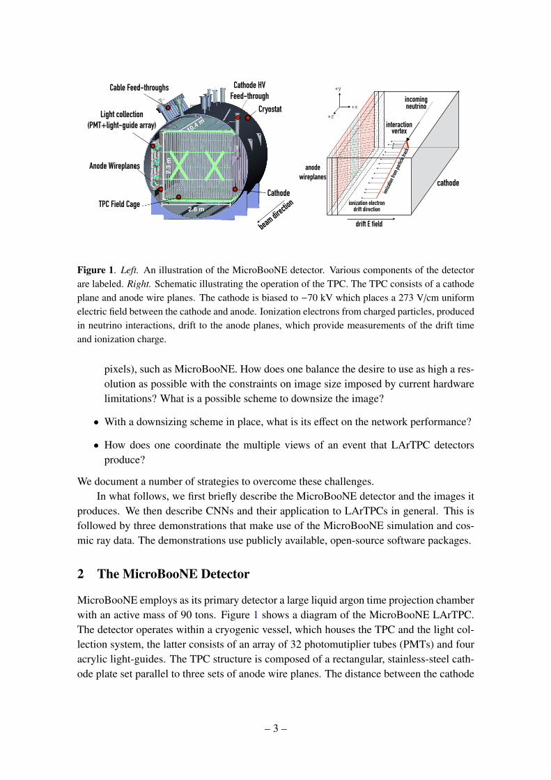
Figure 1. Left. An illustration of the MicroBooNE detector. Various components of the detectorare labeled. Right. Schematic illustrating the operation of the TPC. The TPC consists of a cathodeplane and anode wire planes. The cathode is biased to −70 kV which places a 273 V/cm uniformelectric field between the cathode and anode. Ionization electrons from charged particles, producedin neutrino interactions, drift to the anode planes, which provide measurements of the drift timeand ionization charge.

pixels), such as MicroBooNE. How does one balance the desire to use as high a res-olution as possible with the constraints on image size imposed by current hardwarelimitations? What is a possible scheme to downsize the image?

• With a downsizing scheme in place, what is its effect on the network performance?

• How does one coordinate the multiple views of an event that LArTPC detectorsproduce?

We document a number of strategies to overcome these challenges.In what follows, we first briefly describe the MicroBooNE detector and the images it

produces. We then describe CNNs and their application to LArTPCs in general. This isfollowed by three demonstrations that make use of the MicroBooNE simulation and cos-mic ray data. The demonstrations use publicly available, open-source software packages.

2 The MicroBooNE Detector

MicroBooNE employs as its primary detector a large liquid argon time projection chamberwith an active mass of 90 tons. Figure 1 shows a diagram of the MicroBooNE LArTPC.The detector operates within a cryogenic vessel, which houses the TPC and the light col-lection system, the latter consists of an array of 32 photomutiplier tubes (PMTs) and fouracrylic light-guides. The TPC structure is composed of a rectangular, stainless-steel cath-ode plate set parallel to three sets of anode wire planes. The distance between the cathode

– 3 –

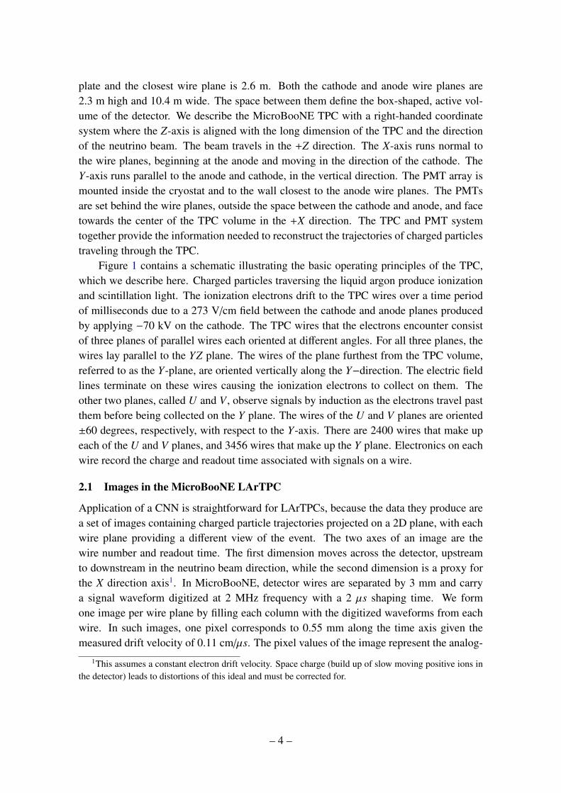
plate and the closest wire plane is 2.6 m. Both the cathode and anode wire planes are2.3 m high and 10.4 m wide. The space between them define the box-shaped, active vol-ume of the detector. We describe the MicroBooNE TPC with a right-handed coordinatesystem where the Z-axis is aligned with the long dimension of the TPC and the directionof the neutrino beam. The beam travels in the +Z direction. The X-axis runs normal tothe wire planes, beginning at the anode and moving in the direction of the cathode. TheY-axis runs parallel to the anode and cathode, in the vertical direction. The PMT array ismounted inside the cryostat and to the wall closest to the anode wire planes. The PMTsare set behind the wire planes, outside the space between the cathode and anode, and facetowards the center of the TPC volume in the +X direction. The TPC and PMT systemtogether provide the information needed to reconstruct the trajectories of charged particlestraveling through the TPC.

Figure 1 contains a schematic illustrating the basic operating principles of the TPC,which we describe here. Charged particles traversing the liquid argon produce ionizationand scintillation light. The ionization electrons drift to the TPC wires over a time periodof milliseconds due to a 273 V/cm field between the cathode and anode planes producedby applying −70 kV on the cathode. The TPC wires that the electrons encounter consistof three planes of parallel wires each oriented at different angles. For all three planes, thewires lay parallel to the YZ plane. The wires of the plane furthest from the TPC volume,referred to as the Y-plane, are oriented vertically along the Y−direction. The electric fieldlines terminate on these wires causing the ionization electrons to collect on them. Theother two planes, called U and V , observe signals by induction as the electrons travel pastthem before being collected on the Y plane. The wires of the U and V planes are oriented±60 degrees, respectively, with respect to the Y-axis. There are 2400 wires that make upeach of the U and V planes, and 3456 wires that make up the Y plane. Electronics on eachwire record the charge and readout time associated with signals on a wire.

2.1 Images in the MicroBooNE LArTPC

Application of a CNN is straightforward for LArTPCs, because the data they produce area set of images containing charged particle trajectories projected on a 2D plane, with eachwire plane providing a different view of the event. The two axes of an image are thewire number and readout time. The first dimension moves across the detector, upstreamto downstream in the neutrino beam direction, while the second dimension is a proxy forthe X direction axis1. In MicroBooNE, detector wires are separated by 3 mm and carrya signal waveform digitized at 2 MHz frequency with a 2 µs shaping time. We formone image per wire plane by filling each column with the digitized waveforms from eachwire. In such images, one pixel corresponds to 0.55 mm along the time axis given themeasured drift velocity of 0.11 cm/µs. The pixel values of the image represent the analog-

1This assumes a constant electron drift velocity. Space charge (build up of slow moving positive ions inthe detector) leads to distortions of this ideal and must be corrected for.

– 4 –

30 cmRun 3469 Event 28734, October 21st, 2015



Figure 2. Example neutrino candidate observed in the MicroBooNE detector. The same interactionis shown in all three wire plane views. The top image is from wire plane U; the middle from wireplane V; and the bottom from wire plane Y . The image is at full resolution and is only from aportion of the full event view.

to-digital-converted (ADC) charge on the wire at the given time tick. ADC counts areencoded over a 12-bit range. This scheme can produce high resolution images for eachwire plane with full charge resolution. In figure 2, we show three images (in false color) ofa neutrino interaction candidate viewed by all three planes as examples of the high qualityinformation obtained by a LArTPC. The task of reconstruction is to parse these images anddetermine information about the neutrino interaction that produced the tracks observed.

The time at which the detector records an image is initiated by external triggers. Eachtrigger defines an event, which is defined as a 4.8 ms period, during which waveformsfrom the TPC wires and the PMTs are recorded. The situation during which the detector istriggered defines the types of events recorded, two of which will be used in our analyses.The first type of event, on-beam events, occurs in synchrony with the arrival of the neutrino

– 5 –

beam at the detector. These events might contain a neutrino interaction. The second type,off-beam events, occur out-of-synchrony with the neutrino beam and should contain onlycosmic-ray trajectories.

For most on-beam events, neutrinos from the beam will pass through the detectorwithout interacting. This means that the vast majority of events collected are uninterestingin the context of a neutrino physics analysis and must be filtered out. The light collectionsystem plays a crucial role in this. Along with ionization, charged particles traversing thedetector will also produce scintillation light coming from the argon. This light is observedby the PMTs within tens of nanoseconds of the interaction time. Thus, the light tells usthe time when the particle passes through the detector. By selecting only those eventswhich have scintillation light occurring in time with the beam, most of the events withoutan interaction are removed. This cut is applied to the event images we analyze. Those thatpass will be referred to as PMT-triggered events.

3 Convolutional Neural Networks

CNNs can be thought of as a modern advancement on feed-forward neural networks(FFNNs), which are commonly employed technique in high energy particle physics anal-yses. CNNs can be seen as a special case of FFNNs, one designed to deal with spatiallylocalized data, such as those found in images. The network architectures of CNNs canbe more complex than those used by FFNNs and include operations that go beyond thoseperformed by the networks’ individual neurons. These extensions have allowed CNNsto become the state-of-the-art solution to many different kinds of problems, most notablyphotographic image classification. CNNs have even begun to find uses in other neutrinoexperiments [4–6] and other LArTPC experiments have ongoing development of deeplearning techniques.

Consider event sample classification, a typical analysis performed by FFNNs in high-energy physics. Here the goal is to assemble a set of N features, calculated for each dataevent, and use them to separate the events in one’s data into C classes. For example, onemight aim to separate the data into a signal-enriched sample and a background-enrichedsample. For many experiments, a common approach to reconstruction is to take raw datafrom various instruments and distill it into several quantities, often focused around charac-terizing observed particles, that can be used to construct these N features. This informationcan then be used to train an FFNN. However, the process of developing reconstruction al-gorithms can often be a long, complicated task. In the case of LArTPCs, we can employCNNs, which can do much of this work automatically by learning its own set of featuresfrom data. This ability of CNNs is due to their architecture, which differs substantiallyfrom that of FFNNs.

In FFNNs, the input feature vector, ~x is passed into one or more hidden layers ofneurons. These hidden layers eventually feed into an output layer containing C neurons,which together produce a C-dimensional output vector, ~y. Figure 3 contains a diagram

– 6 –

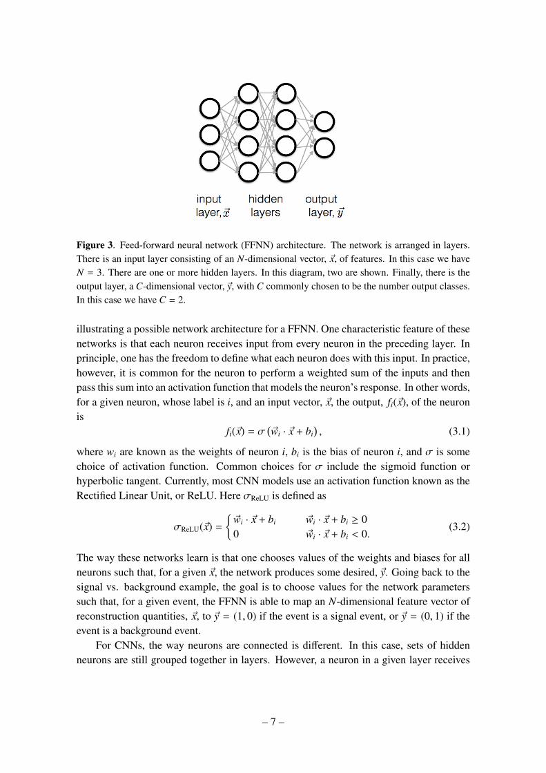
Figure 3. Feed-forward neural network (FFNN) architecture. The network is arranged in layers.There is an input layer consisting of an N-dimensional vector, ~x, of features. In this case we haveN = 3. There are one or more hidden layers. In this diagram, two are shown. Finally, there is theoutput layer, a C-dimensional vector, ~y, with C commonly chosen to be the number output classes.In this case we have C = 2.

illustrating a possible network architecture for a FFNN. One characteristic feature of thesenetworks is that each neuron receives input from every neuron in the preceding layer. Inprinciple, one has the freedom to define what each neuron does with this input. In practice,however, it is common for the neuron to perform a weighted sum of the inputs and thenpass this sum into an activation function that models the neuron’s response. In other words,for a given neuron, whose label is i, and an input vector, ~x, the output, fi(~x), of the neuronis

fi(~x) = σ(~wi · ~x + bi

), (3.1)

where wi are known as the weights of neuron i, bi is the bias of neuron i, and σ is somechoice of activation function. Common choices for σ include the sigmoid function orhyperbolic tangent. Currently, most CNN models use an activation function known as theRectified Linear Unit, or ReLU. Here σReLU is defined as

σReLU(~x) =

{~wi · ~x + bi ~wi · ~x + bi ≥ 00 ~wi · ~x + bi < 0.

(3.2)

The way these networks learn is that one chooses values of the weights and biases for allneurons such that, for a given ~x, the network produces some desired, ~y. Going back to thesignal vs. background example, the goal is to choose values for the network parameterssuch that, for a given event, the FFNN is able to map an N-dimensional feature vector ofreconstruction quantities, ~x, to ~y = (1, 0) if the event is a signal event, or ~y = (0, 1) if theevent is a background event.

For CNNs, the way neurons are connected is different. In this case, sets of hiddenneurons are still grouped together in layers. However, a neuron in a given layer receives

– 7 –

input feature maphidden layers~x

input layer,

output layer, ~y

(a) Feed-forward neural network (b) Feed-forward neural network

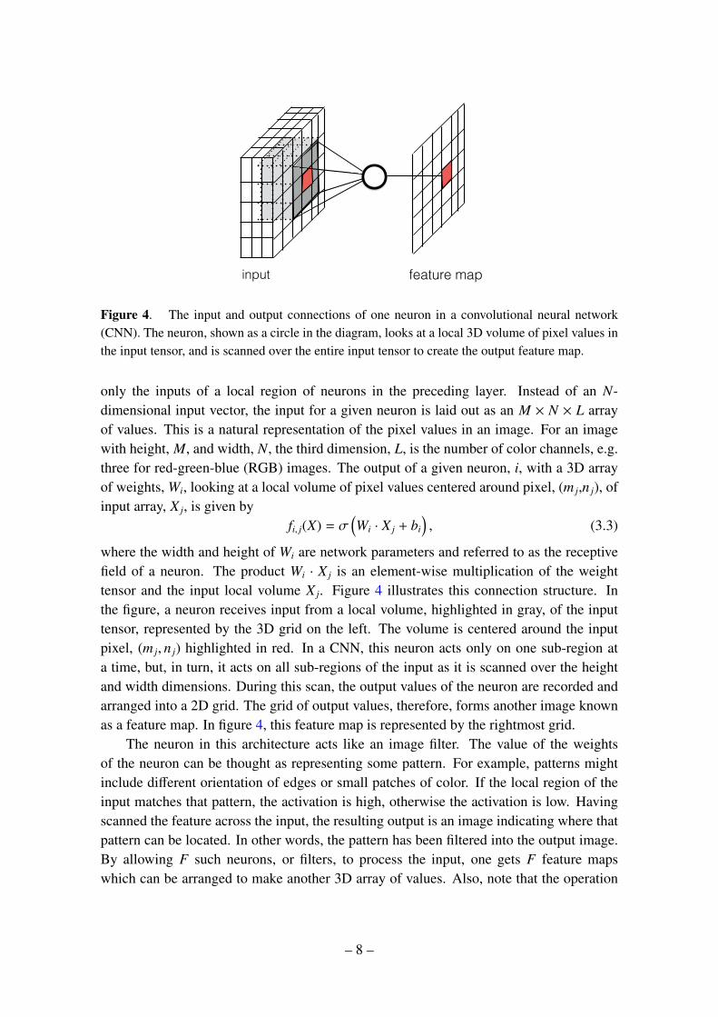
Figure 4. The input and output connections of one neuron in a convolutional neural network(CNN). The neuron, shown as a circle in the diagram, looks at a local 3D volume of pixel values inthe input tensor, and is scanned over the entire input tensor to create the output feature map.

only the inputs of a local region of neurons in the preceding layer. Instead of an N-dimensional input vector, the input for a given neuron is laid out as an M × N × L arrayof values. This is a natural representation of the pixel values in an image. For an imagewith height, M, and width, N, the third dimension, L, is the number of color channels, e.g.three for red-green-blue (RGB) images. The output of a given neuron, i, with a 3D arrayof weights, Wi, looking at a local volume of pixel values centered around pixel, (m j,n j), ofinput array, X j, is given by

fi, j(X) = σ(Wi · X j + bi

), (3.3)

where the width and height of Wi are network parameters and referred to as the receptivefield of a neuron. The product Wi · X j is an element-wise multiplication of the weighttensor and the input local volume X j. Figure 4 illustrates this connection structure. Inthe figure, a neuron receives input from a local volume, highlighted in gray, of the inputtensor, represented by the 3D grid on the left. The volume is centered around the inputpixel, (m j, n j) highlighted in red. In a CNN, this neuron acts only on one sub-region ata time, but, in turn, it acts on all sub-regions of the input as it is scanned over the heightand width dimensions. During this scan, the output values of the neuron are recorded andarranged into a 2D grid. The grid of output values, therefore, forms another image knownas a feature map. In figure 4, this feature map is represented by the rightmost grid.

The neuron in this architecture acts like an image filter. The value of the weightsof the neuron can be thought as representing some pattern. For example, patterns mightinclude different orientation of edges or small patches of color. If the local region of theinput matches that pattern, the activation is high, otherwise the activation is low. Havingscanned the feature across the input, the resulting output is an image indicating where thatpattern can be located. In other words, the pattern has been filtered into the output image.By allowing F such neurons, or filters, to process the input, one gets F feature mapswhich can be arranged to make another 3D array of values. Also, note that the operation

– 8 –

of scanning the neuron across the input is a convolution between the input and the filter.The collection of filters that operate on an input array and produce a set of feature maps isknown as a convolutional layer.

Like FFNNs, one can arrange a CNN as a series of layers where the output of oneconvolutional layer is passed as input to another convolutional layer. With such a stackof layers, CNNs learn to identify high-level objects through combinations of low-levelpatterns. Furthermore, because a given pattern is scanned across the image, translation-invariant features are identified.

This architecture has a couple of advantages. First, the parameters of the neurons,or filters, are learned. Like FFNNs, training the network involves an algorithm whichchooses the parameters of the neurons such that the network learns to map an input imageto some number or vector. This ability to learn its own features is one of the reasons CNNsare so powerful and have seen such widespread use. When approaching a new problem,instead of having to come up with a set of features to extract from the data, with CNNsone can simply collect as much data as possible and start training the network. Second, thenumber of parameters per layer is much smaller than the number of parameters per layerof an FFNN. In an FFNN, each neuron has a weight for all input neurons in the precedinglayer. This is large number of parameters, if one used every pixel of an image as input tothe network. In contrast, the parameters per layer for CNNs is only the volume of localinput region for each filter times the number of filters. This efficient use of parametersallows CNNs to be composed of many, successive convolutional layers. The more layersone uses, the more complex an object can be represented. And currently, the understandingis that “deep” networks with a very large number of layers (on the order of one hundred ormore) tend to work better than shallow networks.

The attractiveness of a machine learning approach is that it might reduce the numberof pattern recognition algorithms that physicists must develop. Likely, different algorithmswill be required for specific types of physics processes. Such algorithms can take manyperson-hours to develop and then optimize for efficient computation. Instead, CNNs po-tentially offer a different strategy, one in which networks are left to discover their ownpatterns to recognize the various processes and other physical quantities of interest. Fur-thermore, processing an image takes on the order of tens of milliseconds on a graphicsprocessing unit (GPU), which should be just as fast, if not faster, than other pattern recog-nition algorithms. However, this approach is still relatively unexplored, and so in this workwe describe three studies, or demonstrations, applying CNNs to LArTPC images.

3.1 Demonstration Steps

We demonstrate the applicability of CNNs through the following tests:

• Demonstration 1– Classification and detection of a simulated single particle withina single-plane image;

– 9 –

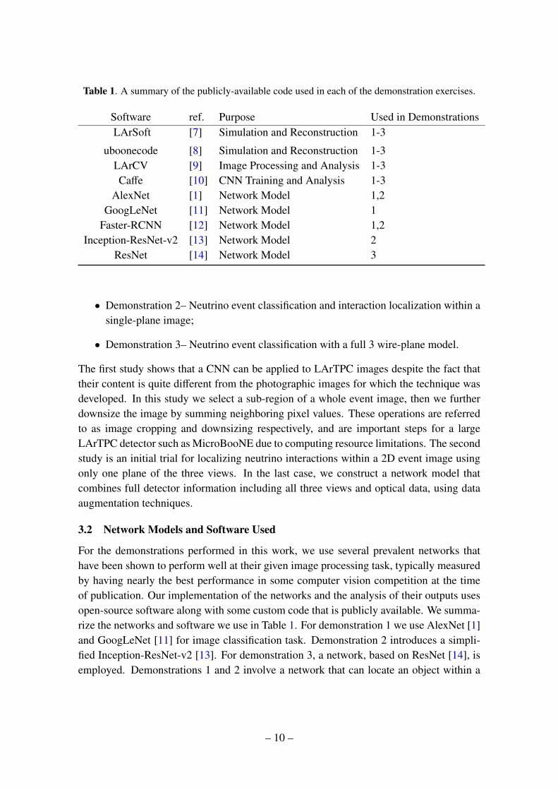
Table 1. A summary of the publicly-available code used in each of the demonstration exercises.

Software ref. Purpose Used in DemonstrationsLArSoft [7] Simulation and Reconstruction 1-3

uboonecode [8] Simulation and Reconstruction 1-3LArCV [9] Image Processing and Analysis 1-3Caffe [10] CNN Training and Analysis 1-3

AlexNet [1] Network Model 1,2GoogLeNet [11] Network Model 1

Faster-RCNN [12] Network Model 1,2Inception-ResNet-v2 [13] Network Model 2

ResNet [14] Network Model 3

• Demonstration 2– Neutrino event classification and interaction localization within asingle-plane image;

• Demonstration 3– Neutrino event classification with a full 3 wire-plane model.

The first study shows that a CNN can be applied to LArTPC images despite the fact thattheir content is quite different from the photographic images for which the technique wasdeveloped. In this study we select a sub-region of a whole event image, then we furtherdownsize the image by summing neighboring pixel values. These operations are referredto as image cropping and downsizing respectively, and are important steps for a largeLArTPC detector such as MicroBooNE due to computing resource limitations. The secondstudy is an initial trial for localizing neutrino interactions within a 2D event image usingonly one plane of the three views. In the last case, we construct a network model thatcombines full detector information including all three views and optical data, using dataaugmentation techniques.

3.2 Network Models and Software Used

For the demonstrations performed in this work, we use several prevalent networks thathave been shown to perform well at their given image processing task, typically measuredby having nearly the best performance in some computer vision competition at the timeof publication. Our implementation of the networks and the analysis of their outputs usesopen-source software along with some custom code that is publicly available. We summa-rize the networks and software we use in Table 1. For demonstration 1 we use AlexNet [1]and GoogLeNet [11] for image classification task. Demonstration 2 introduces a simpli-fied Inception-ResNet-v2 [13]. For demonstration 3, a network, based on ResNet [14], isemployed. Demonstrations 1 and 2 involve a network that can locate an object within a

– 10 –

sub-region of an image (Region of Interest, or ROI, finding). For this task we use a networkknown as the Faster-region convolutional neural network, or Faster-RCNN [12].

All of the above models are CNNs with various depths of layers. The choice ofAlexNet for demonstrations 1 and 2 is motivated by the fact that this relatively shallowmodel is often used as a benchmark in the field of computer vision ever since it was firstintroduced for the annual Large Scale Vision Recognition Challenge (LSVRC) in 2012.GoogLeNet, which has 22 layers compared to 8 layers in AlexNet, is another popularmodel which we employed to compare to AlexNet in demonstration 1.

Faster-RCNN, the state-of-the-art object detection network used in demonstrations 1and 2, can identify multiple instances of different object classes within the same image. Inthis paper we combine this architecture with AlexNet for object detection networks taskedwith locating various particle types or a neutrino interaction in a given event image.

We also use truncated versions of two networks, ResNet [14] and Inception-ResNet-v2 [13], to perform neutrino event classification in demonstrations 2 and 3. Both networksuse a type of sub-network architecture know as residual convolutional modules introducedin ref. [14]. These modules are believed to help the network achieve higher accuracy andlearn faster. (For a description of a residual model, see ref. [14] or appendix A.)

Throughout all studies in this work, we use one of the most popular open-source CNNsoftware frameworks, Caffe [10], for CNN training and analysis. Input data is in a ROOTfile format [15] created by the LArCV software framework [9], which we developed toact as the interface between LArSoft and Caffe. LArCV is also an image data processingframework and is used to further process and analyze images as described in the followingsections. One can find our custom version of Caffe that utilizes the LArCV framework in[9].

The computing hardware used in this study involves a server machine equipped withtwo NVIDIA Titan X GPU cards [16], chosen in part due to their large amounts of on-board memory (12 GB). We have two such servers of similar specifications at the Mas-sachusetts Institute of Technology and at Columbia University, which are used for trainingand analysis tasks.

4 Demonstration 1: Single Particle Classification and Detection

In this demonstration, we investigate the ability of CNNs to classify images of singleparticles located in various regions of the MicroBooNE detector. We show that CNNs canlocate particles by specifying a bounding box that contains the particle. This demonstrationalso proposes a strategy for working with the large image sizes from large LArTPCs. Thedetector creates three images per event, one from each plane, which at full resolutionhave dimensions of either 2400 wires × 9600 digitized time ticks for the induction planes,U and V , or 3456 wires × 9600 time ticks for the collection plane, Y . Future LArTPCexperiments will produce similar size or even larger images. Such images are too large to

– 11 –

use for training a CNN of reasonable size on any GPU card available on the market. Tomitigate this problem one must crop or downsize the image, or possibly both.

Therefore, in demonstration 1, we study the following things.

1. The performance of five particle classification (e−, γ, µ−, π−, proton) CNNs, usingAlexNet and GoogLeNet as our nework models, applied to cropped, high-resolutionimages.

2. A comparison of the above with low-resolution images (that have been downsizedby a factor of two in both pixel axes).

3. Two-particle separation for e−/γ and µ−/π−.

4. The performance of a CNN to draw a bounding box around the single particles.

The first task serves as a proof-of-principle that CNNs have the capability to interpretLArTPC images. The second is a comparison of how the downsizing factor affects ourclassification capability. The third focuses on particular cases interesting to the LArTPCcommunity. Finally, the fourth is a simple test case of applying an object detection net-work, Faster-RCNN [12], to LArTPC images.

4.1 Sample Preparation

4.1.1 Producing Images

For this study, we generated images using a single particle simulation built upon LAr-Soft [7], a simulation and analysis framework written specifically for LArTPC exper-iments. LArSoft uses geant4 [17] for particle tracking. LArSoft also implements amodel of the electron drift inside the liquid argon medium. Each event for this demonstra-tion simulates only one particle: e−, γ, µ−, π−, or proton. Particles are generated uniformlyinside the TPC active volume. Their momenta are distributed uniformly between 100 MeVand 1 GeV, except for protons which were generated with kinetic energy distributed uni-formly between 100 MeV and 788 MeV where the upper bound is set to cover about thesame momentum range, 1 GeV/c, of the other particles. The particles’ initial directionsare generated in an isotropic manner. After their location and kinematics are determined,the particles are passed to geant4 for tracking.

After the events are tracked by geant4, the MicroBooNE detector simulation, alsobuilt upon LArSoft, is used to generate signals on all the MicroBooNE wires. This isdone with the 3D pattern of ionization deposited by charged particles within the TPC. Thedetector simulation uses the deposited charge to simulate the signals on the wires using amodel for the electron drift that includes diffusion and ionization lost to impurities. Thismodel provides a distribution of charge at the wire planes which then goes into simulatingthe expected raw, digitized signals on the wires. These raw signals are based on 2D sim-ulations of charge propagation and electronics response on the induction and collectionplanes. We then convert these raw wire signals into an image.

– 12 –

The conversion of wire signals to an image, both for the simulation and for detectordata used in later demonstrations, proceeds through the following steps. First, the digi-tized, raw wire signals are sent through a noise filter [18]. Then, they are passed throughan algorithm which converts the filtered, raw signals into calibrated signals [19]. Thevalues of the calibrated, digitized waveforms then populate a 1-channel image, i.e. a 2Darray, with one axis being time and the other being a sequence of wires. We form an imagefor each of the three wire planes. Because the Y plane has more wires than the U and Vplanes, a full event image for each plane has a width of 3456 pixels. For the U and Vplanes, which only have 2400 wires, the first 2400 pixels are filled, while the rest are setto zero. As a technical aside, we note that the value of each pixel is stored as a float as thatis one of the input choices for Caffe. We do not convert the ADC values into 8-bit valuestypical of natural images.

A full MicroBooNE event has a total of 9600 time ticks. For this and the other demon-strations, we use a 6048 time tick subset ranging from tick 2400 to 8448 with respect tothe first tick of the full event. This subset includes time before and after the expected sig-nal region. A reason to include these extra time ranges is to demonstrate that the analysismethodology employed in this study can be used for neutrino analysis in the future withthe same hardware resources we have today. Particles are generated at a time which cor-responds to the time tick 800 in the recorded readout waveform, and all associated chargedeposition is expected to reach the readout wire plane by time tick 5855 given the by driftvelocity. Finally, this simulation includes a list of unresponsive wires, which carry nowaveform. In total, about 830 (or 10%) of the wires in the detector are labeled as unre-sponsive [18]. The number of such wires on the U plane is about 400, on the V plane about100, and on the Y plane about 330. This list of wires is created based on real detector data.

Following a sample generation of images composed of 3456 wires and 6048 timeticks, we downsize by a factor of two in wire and six in time to produce a resulting imagesize of 1728×1008 pixels. We downsize by merging pixels through a simple sum of pixelvalues. Although this causes a loss of resolution and, therefore, a loss of information, par-ticularly along the wire axis, it is necessary due to hardware memory limitation. Howeverthe loss of information is smaller than one would naively expected in the time directionbecause the digitization period is shorter than the electronics shaping time, which is 2microseconds, or 4 time ticks.

Next, we run an algorithm in the LArCV package, referred to as HiResDivider,whose purpose is to divide the three, whole-event images into sets of three-plane sub-images where the set of sub-images views the same region of the detector over the sametime period. The algorithm is configured to produce sets of sub-images that are 576×576pixels. Note that while this demonstration only uses images from the Y plane, such amethod will be useful for future work with large LArTPC images as it is a way to workwith smaller images. The algorithm first sub-divides the whole detector active volume intoa number of equally sized 3D boxes, and then crops around the wires that read out that 3Dregion. For our study, we find the 3D box that contains the start of a particle trajectory and

– 13 –

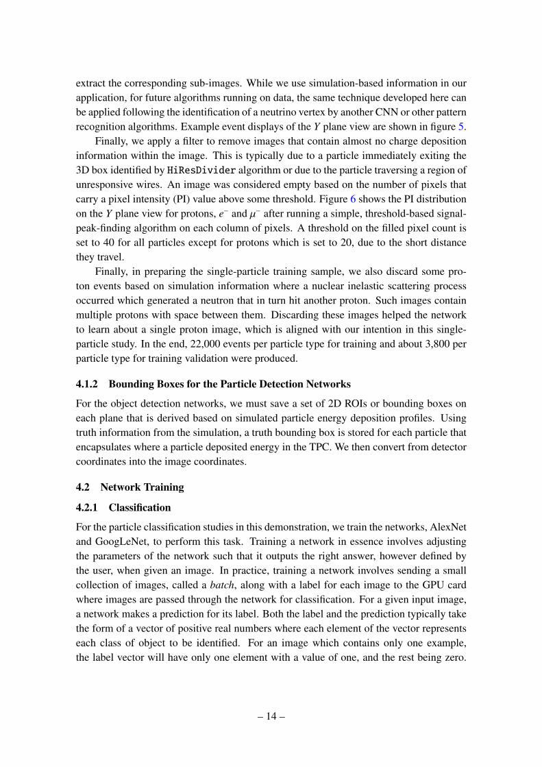
extract the corresponding sub-images. While we use simulation-based information in ourapplication, for future algorithms running on data, the same technique developed here canbe applied following the identification of a neutrino vertex by another CNN or other patternrecognition algorithms. Example event displays of the Y plane view are shown in figure 5.

Finally, we apply a filter to remove images that contain almost no charge depositioninformation within the image. This is typically due to a particle immediately exiting the3D box identified by HiResDivider algorithm or due to the particle traversing a region ofunresponsive wires. An image was considered empty based on the number of pixels thatcarry a pixel intensity (PI) value above some threshold. Figure 6 shows the PI distributionon the Y plane view for protons, e− and µ− after running a simple, threshold-based signal-peak-finding algorithm on each column of pixels. A threshold on the filled pixel count isset to 40 for all particles except for protons which is set to 20, due to the short distancethey travel.

Finally, in preparing the single-particle training sample, we also discard some pro-ton events based on simulation information where a nuclear inelastic scattering processoccurred which generated a neutron that in turn hit another proton. Such images containmultiple protons with space between them. Discarding these images helped the networkto learn about a single proton image, which is aligned with our intention in this single-particle study. In the end, 22,000 events per particle type for training and about 3,800 perparticle type for training validation were produced.

4.1.2 Bounding Boxes for the Particle Detection Networks

For the object detection networks, we must save a set of 2D ROIs or bounding boxes oneach plane that is derived based on simulated particle energy deposition profiles. Usingtruth information from the simulation, a truth bounding box is stored for each particle thatencapsulates where a particle deposited energy in the TPC. We then convert from detectorcoordinates into the image coordinates.

4.2 Network Training

4.2.1 Classification

For the particle classification studies in this demonstration, we train the networks, AlexNetand GoogLeNet, to perform this task. Training a network in essence involves adjustingthe parameters of the network such that it outputs the right answer, however defined bythe user, when given an image. In practice, training a network involves sending a smallcollection of images, called a batch, along with a label for each image to the GPU cardwhere images are passed through the network for classification. For a given input image,a network makes a prediction for its label. Both the label and the prediction typically takethe form of a vector of positive real numbers where each element of the vector representseach class of object to be identified. For an image which contains only one example,the label vector will have only one element with a value of one, and the rest being zero.

– 14 –

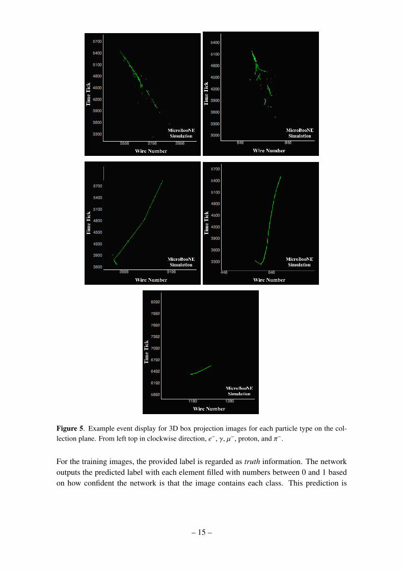
Figure 5. Example event display for 3D box projection images for each particle type on the col-lection plane. From left top in clockwise direction, e−, γ, µ−, proton, and π−.

For the training images, the provided label is regarded as truth information. The networkoutputs the predicted label with each element filled with numbers between 0 and 1 basedon how confident the network is that the image contains each class. This prediction is

– 15 –

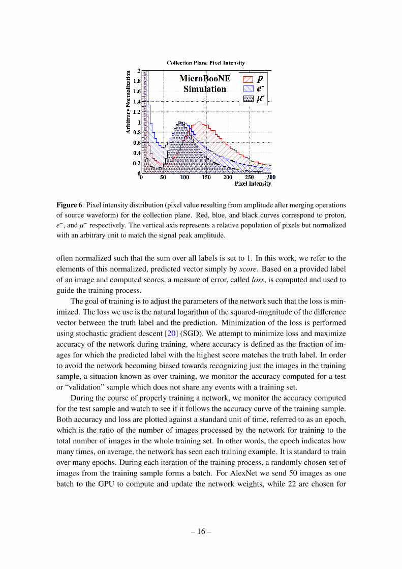
Figure 6. Pixel intensity distribution (pixel value resulting from amplitude after merging operationsof source waveform) for the collection plane. Red, blue, and black curves correspond to proton,e−, and µ− respectively. The vertical axis represents a relative population of pixels but normalizedwith an arbitrary unit to match the signal peak amplitude.

often normalized such that the sum over all labels is set to 1. In this work, we refer to theelements of this normalized, predicted vector simply by score. Based on a provided labelof an image and computed scores, a measure of error, called loss, is computed and used toguide the training process.

The goal of training is to adjust the parameters of the network such that the loss is min-imized. The loss we use is the natural logarithm of the squared-magnitude of the differencevector between the truth label and the prediction. Minimization of the loss is performedusing stochastic gradient descent [20] (SGD). We attempt to minimize loss and maximizeaccuracy of the network during training, where accuracy is defined as the fraction of im-ages for which the predicted label with the highest score matches the truth label. In orderto avoid the network becoming biased towards recognizing just the images in the trainingsample, a situation known as over-training, we monitor the accuracy computed for a testor “validation” sample which does not share any events with a training set.

During the course of properly training a network, we monitor the accuracy computedfor the test sample and watch to see if it follows the accuracy curve of the training sample.Both accuracy and loss are plotted against a standard unit of time, referred to as an epoch,which is the ratio of the number of images processed by the network for training to thetotal number of images in the whole training set. In other words, the epoch indicates howmany times, on average, the network has seen each training example. It is standard to trainover many epochs. During each iteration of the training process, a randomly chosen set ofimages from the training sample forms a batch. For AlexNet we send 50 images as onebatch to the GPU to compute and update the network weights, while 22 are chosen for

– 16 –

Figure 7. Network training loss (left column) and accuracy (right column) for AlexNet (top row)and GoogLeNet (bottom row). The horizontal axis denotes elapsed time since the start of training.Blue data points are computed within the training process per batch of images. Red data pointsare computed by taking an average of 100 consecutive blue data points. The magenta data pointson the accuracy curve are computed using a validation sample to identify over-training. At aroundepoch 3 the learning rate of the network has been reduced for fine tuning. This results in a step ofdecrease in the loss and increase in the network accuracy.

GoogLeNet. These batch sizes are chosen based on the network size and GPU memorylimitations. After the network is loaded into the memory of the GPU, we choose a batchsize that maximizes the usage of the remaining memory on the GPU. Figure 7 shows boththe loss and accuracy curves during the training process of the five particle classificationtask. The observed curves are consistent with what one would expect during an acceptabletraining course.

In addition, for classification tasks, we train the networks with lower resolution im-ages where the training and test images were downsized by a factor of two in both wiresand time ticks to study how the network performance changes. As a final test, we train bothAlexNet and GoogLeNet for a two-particle classification task using only a sample consist-ing of µ− and π− images. This is to compare µ− versus π− separation performance betweennetworks trained on a sample containing only two particles versus the five-particle sample,where in the latter the network is exposed to a richer variety of features.

– 17 –

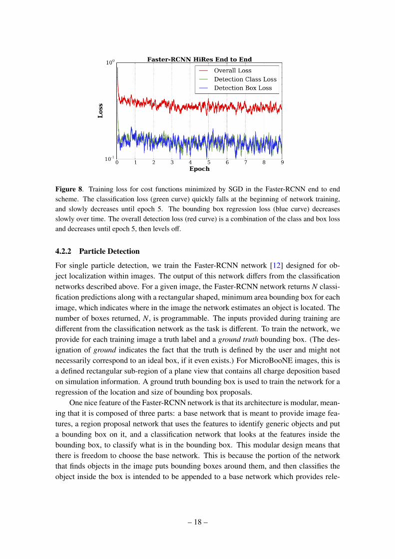
Figure 8. Training loss for cost functions minimized by SGD in the Faster-RCNN end to endscheme. The classification loss (green curve) quickly falls at the beginning of network training,and slowly decreases until epoch 5. The bounding box regression loss (blue curve) decreasesslowly over time. The overall detection loss (red curve) is a combination of the class and box lossand decreases until epoch 5, then levels off.

4.2.2 Particle Detection

For single particle detection, we train the Faster-RCNN network [12] designed for ob-ject localization within images. The output of this network differs from the classificationnetworks described above. For a given image, the Faster-RCNN network returns N classi-fication predictions along with a rectangular shaped, minimum area bounding box for eachimage, which indicates where in the image the network estimates an object is located. Thenumber of boxes returned, N, is programmable. The inputs provided during training aredifferent from the classification network as the task is different. To train the network, weprovide for each training image a truth label and a ground truth bounding box. (The des-ignation of ground indicates the fact that the truth is defined by the user and might notnecessarily correspond to an ideal box, if it even exists.) For MicroBooNE images, this isa defined rectangular sub-region of a plane view that contains all charge deposition basedon simulation information. A ground truth bounding box is used to train the network for aregression of the location and size of bounding box proposals.

One nice feature of the Faster-RCNN network is that its architecture is modular, mean-ing that it is composed of three parts: a base network that is meant to provide image fea-tures, a region proposal network that uses the features to identify generic objects and puta bounding box on it, and a classification network that looks at the features inside thebounding box, to classify what is in the bounding box. This modular design means thatthere is freedom to choose the base network. This is because the portion of the networkthat finds objects in the image puts bounding boxes around them, and then classifies theobject inside the box is intended to be appended to a base network which provides rele-

– 18 –

vant image features. In this study, we used AlexNet trained for five particle classificationdescribed above as the base network. We append the Faster-RCNN portion of the net-work after the fifth convolutional layer of AlexNet. We transfer the parameters from theclassification portion of AlexNet and use them to initialize the classification portion of theFaster-RCNN network since it will be asked to identify the same classes of objects. Wetrain the whole network in the approximate joint training scheme [12] with stochastic gra-dient descent. The loss minimized for the Faster-RCNN comes from both object detectionand classification tasks. This multi-task loss over the course of our training is shown inFigure 8. We assess the performance of the detection network in a later subsection.

4.3 Five Particle Classification Performance

Figure 9 shows the classification performance using the network trained on the 5 particletypes described in section 4.1 using image sizes of 576 by 576 pixels. Each plot in thefigure corresponds to a sample of events of a specific particle type, and the distributionshows the fraction of events classified as each of the 5 particle types, given by the highestscore for each hypothesis. A result using images that have been further downsized by afactor of 2 is shown in figure 10. The classification performance for each particle type aswell as the most mis-identified particle types, with mis-identifying score, are summarizedin tables 2 and 3.

Learning Geometrical Shapes The networks have clearly learned about geometricalshapes of showers and tracks irrespective of image downsizing. Both figures 9 and 10show that the network is more likely to be confused among track-shaped particles (µ−, π−,and proton) and also among shower-shaped particles (e− and γ) but less between thosecategories.

Learning dE/dx e− and γ have similar geometrical shapes, i.e. they produce showers,but differ in the energy deposited per unit length, called dE/dx, near the starting point ofthe shower. The fact the network can separate these two particles fairly well may meanthe network has learned about this difference, or some other difference in the gamma andelectron shower development. It is also worth noting that downsizing an image worsens theresult, likely because downsizing, which involves combining neighboring pixels, smearsout the dE/dx information.

Network Depth We expect GoogLeNet to be capable of learning more features thanAlexNet overall, because of its more advanced, deeper model. Our results are consistentwith this expectation as can be seen in the results table (Table 2). However when compar-ing how AlexNet and GoogLeNet are affected by downsizing an image, it is interesting tonote that AlexNet performs better for those particles with higher dE/dx (γ and proton),which suggests AlexNet is using the dE/dx information more effectively than GoogLeNetafter image is downsized by a factor of 2.

– 19 –

Classified Particle Type

Image, Network e− [%] γ [%] µ− [%] π− [%] proton [%]

HiRes, AlexNet 73.6 ± 0.7 81.3 ± 0.6 84.8 ± 0.6 73.1 ± 0.7 87.2 ± 0.5

LoRes, AlexNet 64.1 ± 0.8 77.3 ± 0.7 75.2 ± 0.7 74.2 ± 0.7 85.8 ± 0.6

HiRes, GoogLeNet 77.8 ± 0.7 83.4 ± 0.6 89.7 ± 0.5 71.0 ± 0.7 91.2 ± 0.5

LoRes, GoogLeNet 74.0 ± 0.7 74.0 ± 0.7 84.1 ± 0.6 75.2 ± 0.7 84.6 ± 0.6

Table 2. Five particle classification performances. The very left column describes the image typeand network where HiRes refers to a standard 576 by 576 pixel image while LowRes refers toa downsized image of 288 by 288 pixels. The five remaining columns denote the classificationperformance per particle type. Quoted uncertainties are purely statistical and assume a binomialdistribution.

Classified Particle Type

Image, Network e− [%] γ [%] µ− [%] π− [%] proton [%]

HiRes, AlexNet γ 23.0 e− 16.2 π− 8.0 µ− 19.8 µ− 7.0

LoRes, AlexNet γ 29.3 e− 17.6 π− 11.7 µ− 16.5 µ− 7.9

HiRes, GoogLeNet γ 19.9 e− 15.0 π− 5.4 µ− 22.6 µ− 4.6

LoRes, GoogLeNet γ 21.0 e− 21.3 π− 9.4 µ− 19.3 µ− 9.1

Table 3. The most frequently misidentified particle type for the five particle classification task.Following table 2, the very left column describes the image type and network where HiRes refersto a standard 576 by 576 pixel image while LowRes refers to a downsized image of 288 by 288pixels. The five remaining columns denote the classification performance per particle type. Eachtable element denotes the most frequently mistaken particle type and its mis-identification rate.

– 20 –

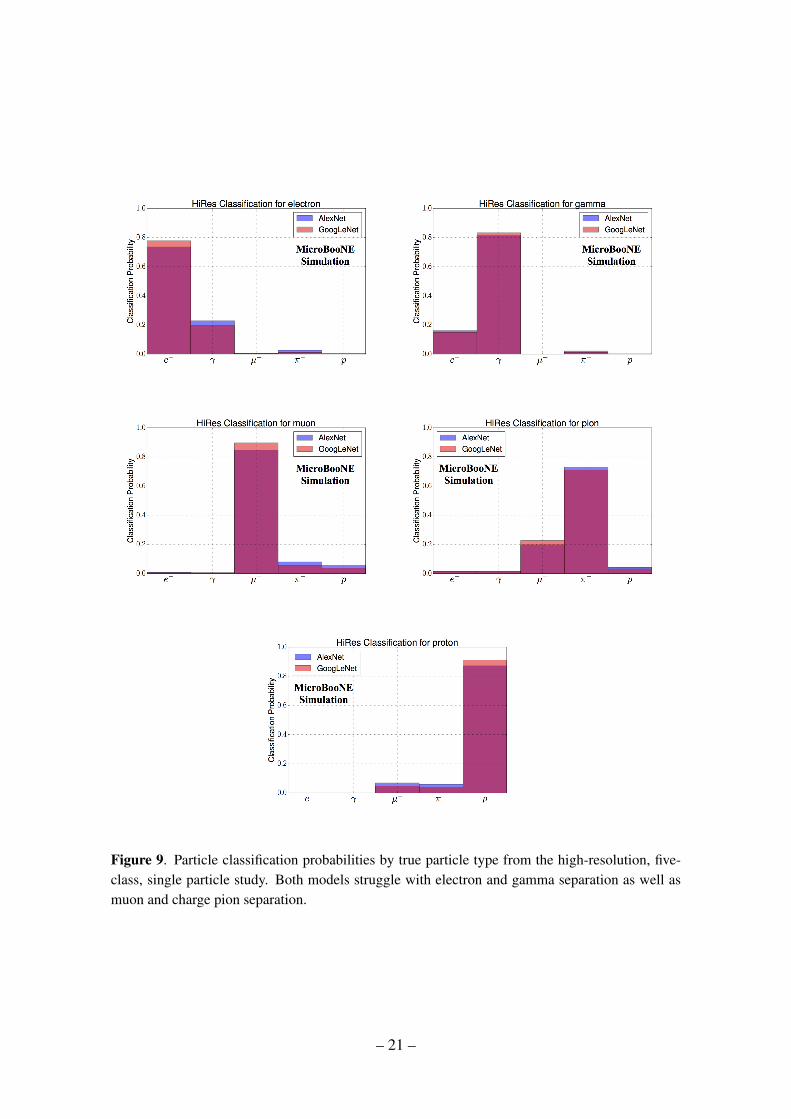
Figure 9. Particle classification probabilities by true particle type from the high-resolution, five-class, single particle study. Both models struggle with electron and gamma separation as well asmuon and charge pion separation.

– 21 –

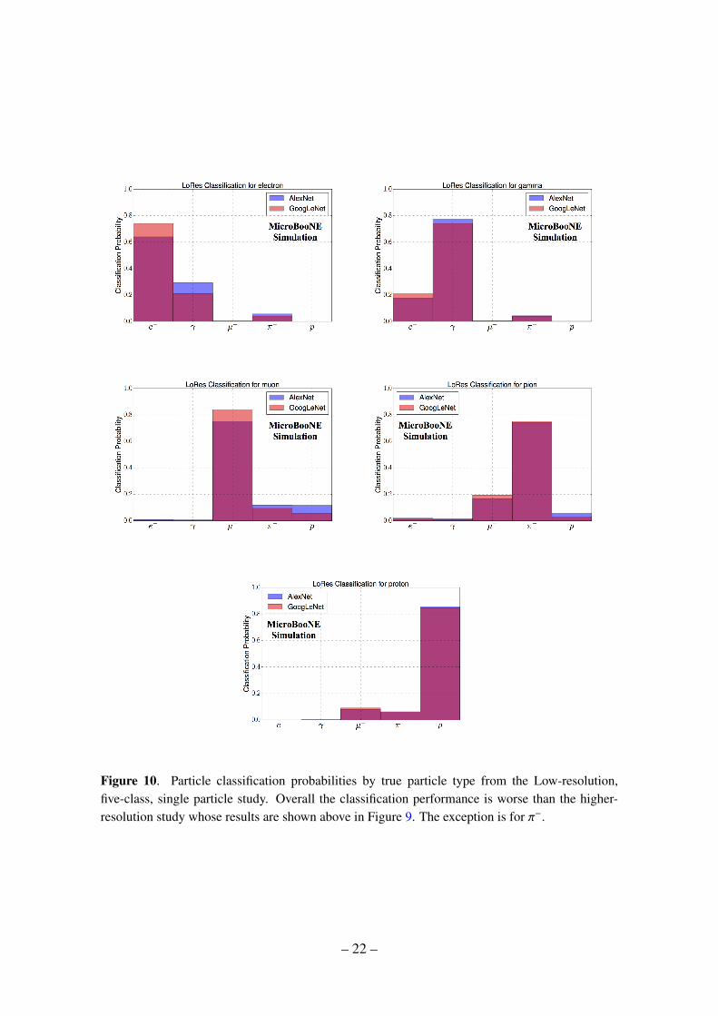
Figure 10. Particle classification probabilities by true particle type from the Low-resolution,five-class, single particle study. Overall the classification performance is worse than the higher-resolution study whose results are shown above in Figure 9. The exception is for π−.

– 22 –

4.4 π−/µ− Separation

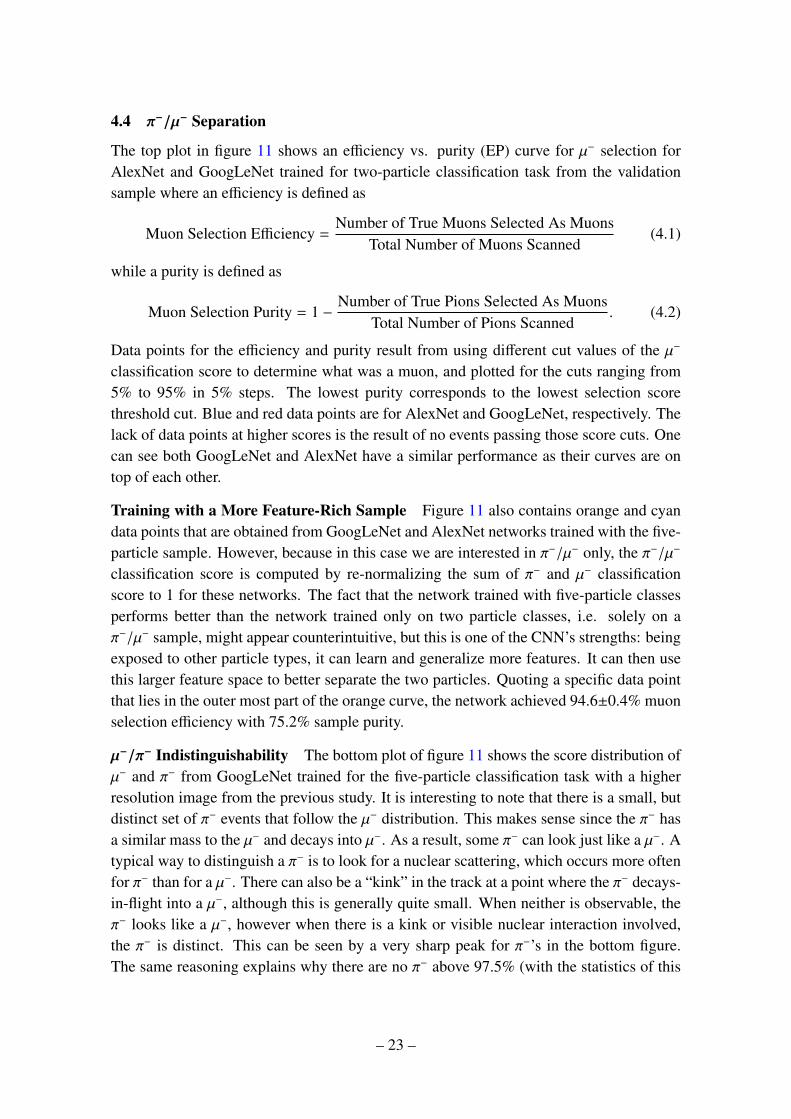
The top plot in figure 11 shows an efficiency vs. purity (EP) curve for µ− selection forAlexNet and GoogLeNet trained for two-particle classification task from the validationsample where an efficiency is defined as

Muon Selection Efficiency =Number of True Muons Selected As Muons

Total Number of Muons Scanned(4.1)

while a purity is defined as

Muon Selection Purity = 1 −Number of True Pions Selected As Muons

Total Number of Pions Scanned. (4.2)

Data points for the efficiency and purity result from using different cut values of the µ−

classification score to determine what was a muon, and plotted for the cuts ranging from5% to 95% in 5% steps. The lowest purity corresponds to the lowest selection scorethreshold cut. Blue and red data points are for AlexNet and GoogLeNet, respectively. Thelack of data points at higher scores is the result of no events passing those score cuts. Onecan see both GoogLeNet and AlexNet have a similar performance as their curves are ontop of each other.

Training with a More Feature-Rich Sample Figure 11 also contains orange and cyandata points that are obtained from GoogLeNet and AlexNet networks trained with the five-particle sample. However, because in this case we are interested in π−/µ− only, the π−/µ−

classification score is computed by re-normalizing the sum of π− and µ− classificationscore to 1 for these networks. The fact that the network trained with five-particle classesperforms better than the network trained only on two particle classes, i.e. solely on aπ−/µ− sample, might appear counterintuitive, but this is one of the CNN’s strengths: beingexposed to other particle types, it can learn and generalize more features. It can then usethis larger feature space to better separate the two particles. Quoting a specific data pointthat lies in the outer most part of the orange curve, the network achieved 94.6±0.4% muonselection efficiency with 75.2% sample purity.

µ−/π− Indistinguishability The bottom plot of figure 11 shows the score distribution ofµ− and π− from GoogLeNet trained for the five-particle classification task with a higherresolution image from the previous study. It is interesting to note that there is a small, butdistinct set of π− events that follow the µ− distribution. This makes sense since the π− hasa similar mass to the µ− and decays into µ−. As a result, some π− can look just like a µ−. Atypical way to distinguish a π− is to look for a nuclear scattering, which occurs more oftenfor π− than for a µ−. There can also be a “kink” in the track at a point where the π− decays-in-flight into a µ−, although this is generally quite small. When neither is observable, theπ− looks like a µ−, however when there is a kink or visible nuclear interaction involved,the π− is distinct. This can be seen by a very sharp peak for π−’s in the bottom figure.The same reasoning explains why there are no π− above 97.5% (with the statistics of this

– 23 –

MicroBooNESimulation


Figure 11. Top: µ− selection EP curve for µ− and π− images produced from the validation sam-ple. Blue and red data points are AlexNet and GoogLeNet respectively trained with a sample setthat only contain π− and µ− as described in section 4.4. Orange and cyan data points are fromGoogLeNet and AlexNet respectively, trained for five particle classification. Bottom: µ− score dis-tribution from GoogLeNet trained for five particle classification where the score is re-normalizedfor the purpose of µ−/π− separation.

sample) because a µ− can never be completely distinguished from the small fraction of π−

that neither decay nor participate in a nuclear scatter.

4.5 e−/γ Separation

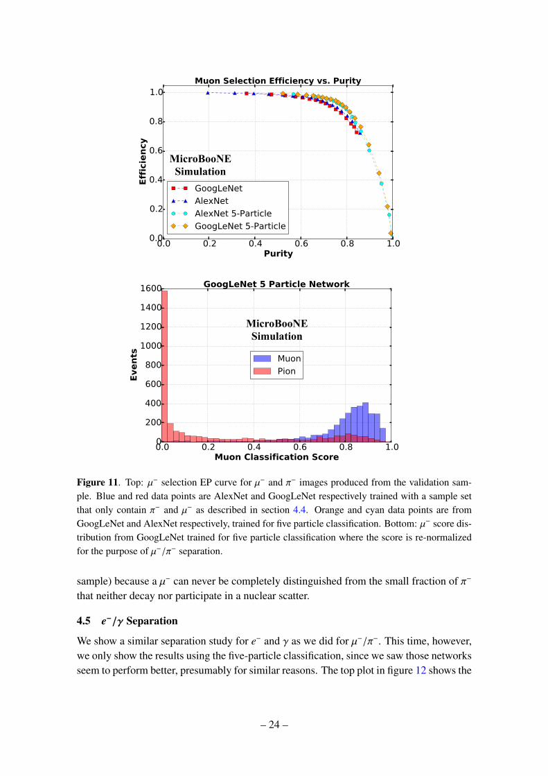
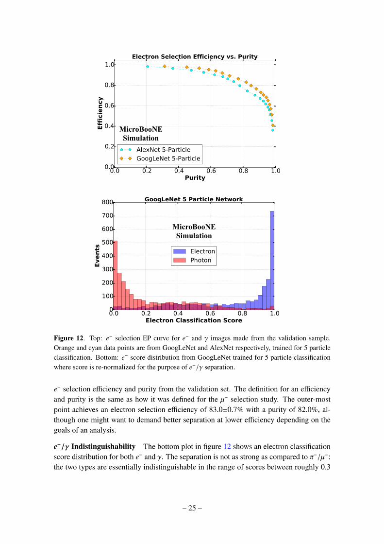
We show a similar separation study for e− and γ as we did for µ−/π−. This time, however,we only show the results using the five-particle classification, since we saw those networksseem to perform better, presumably for similar reasons. The top plot in figure 12 shows the

– 24 –



Figure 12. Top: e− selection EP curve for e− and γ images made from the validation sample.Orange and cyan data points are from GoogLeNet and AlexNet respectively, trained for 5 particleclassification. Bottom: e− score distribution from GoogLeNet trained for 5 particle classificationwhere score is re-normalized for the purpose of e−/γ separation.

e− selection efficiency and purity from the validation set. The definition for an efficiencyand purity is the same as how it was defined for the µ− selection study. The outer-mostpoint achieves an electron selection efficiency of 83.0±0.7% with a purity of 82.0%, al-though one might want to demand better separation at lower efficiency depending on thegoals of an analysis.

e−/γ Indistinguishability The bottom plot in figure 12 shows an electron classificationscore distribution for both e− and γ. The separation is not as strong as compared to π−/µ−:the two types are essentially indistinguishable in the range of scores between roughly 0.3

– 25 –

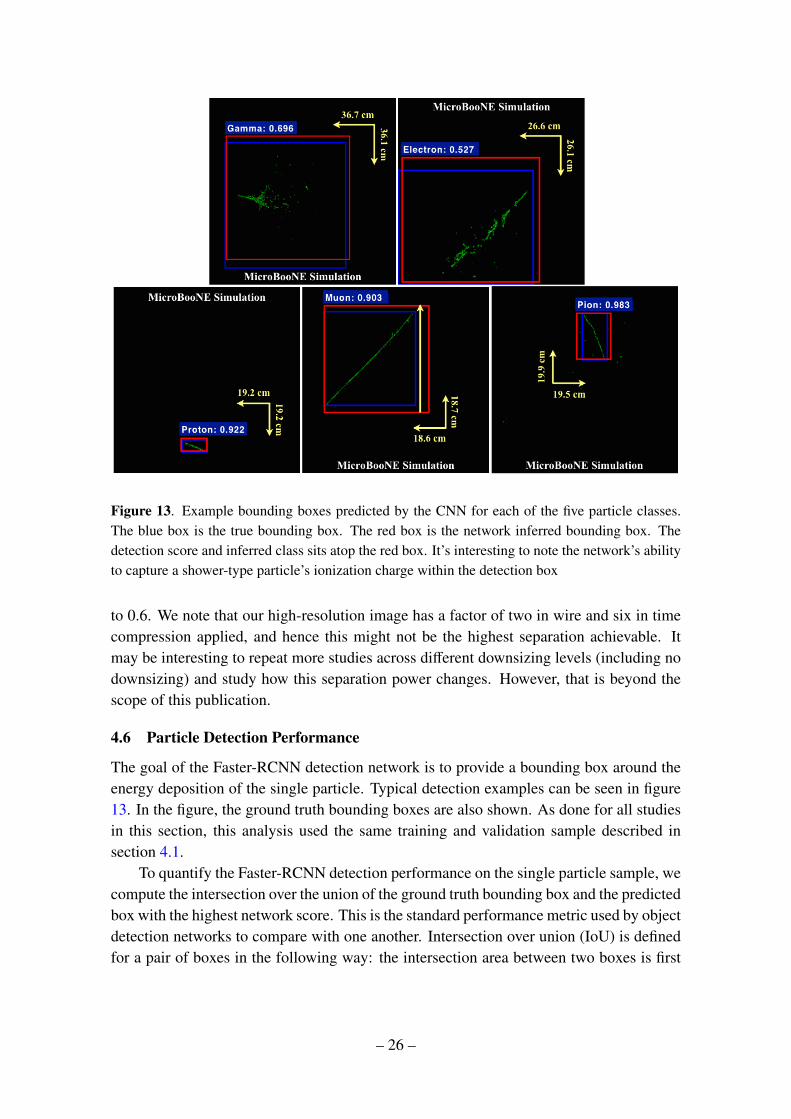
Figure 13. Example bounding boxes predicted by the CNN for each of the five particle classes.The blue box is the true bounding box. The red box is the network inferred bounding box. Thedetection score and inferred class sits atop the red box. It’s interesting to note the network’s abilityto capture a shower-type particle’s ionization charge within the detection box

to 0.6. We note that our high-resolution image has a factor of two in wire and six in timecompression applied, and hence this might not be the highest separation achievable. Itmay be interesting to repeat more studies across different downsizing levels (including nodownsizing) and study how this separation power changes. However, that is beyond thescope of this publication.

4.6 Particle Detection Performance

The goal of the Faster-RCNN detection network is to provide a bounding box around theenergy deposition of the single particle. Typical detection examples can be seen in figure13. In the figure, the ground truth bounding boxes are also shown. As done for all studiesin this section, this analysis used the same training and validation sample described insection 4.1.

To quantify the Faster-RCNN detection performance on the single particle sample, wecompute the intersection over the union of the ground truth bounding box and the predictedbox with the highest network score. This is the standard performance metric used by objectdetection networks to compare with one another. Intersection over union (IoU) is definedfor a pair of boxes in the following way: the intersection area between two boxes is first

– 26 –

computed by calculating the overlap area and then dividing by the difference between thetotal area of the two boxes and their intersection area. Specifically for two boxes with areaA1 and A2,

IoU =A1 ∩ A2

A1 + A2 − A1 ∩ A2. (4.3)

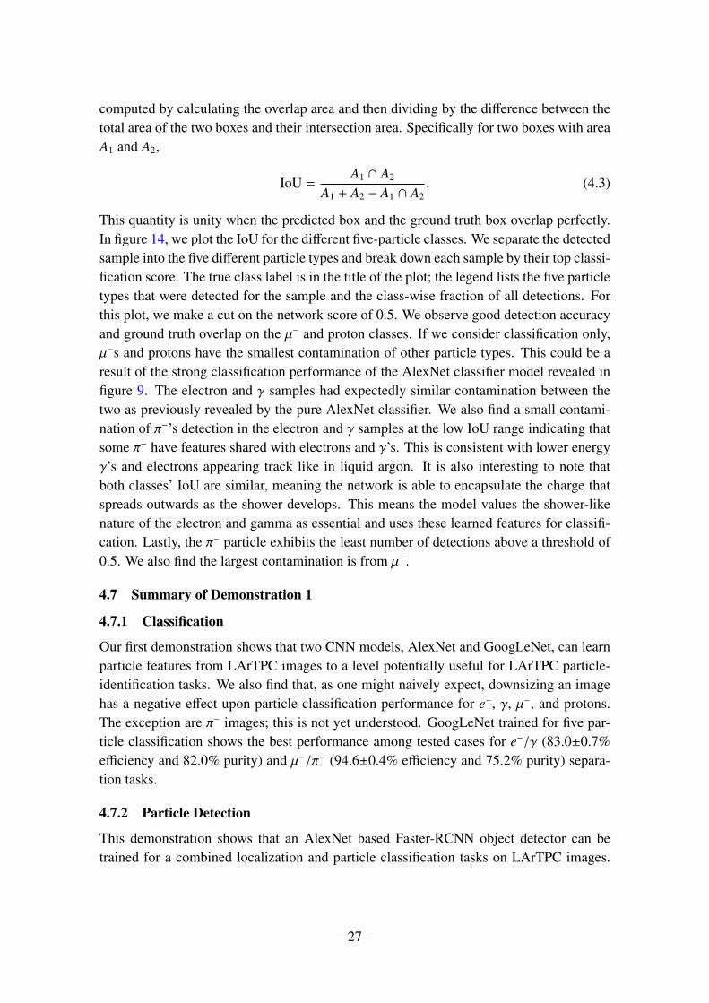
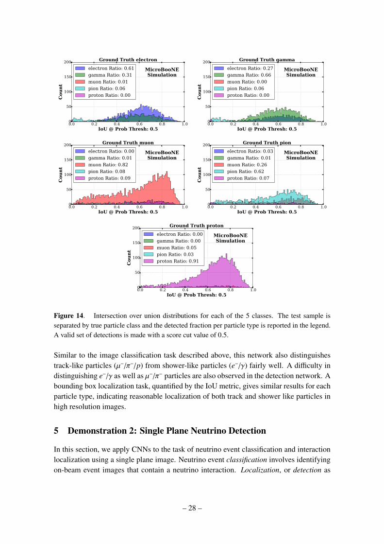
This quantity is unity when the predicted box and the ground truth box overlap perfectly.In figure 14, we plot the IoU for the different five-particle classes. We separate the detectedsample into the five different particle types and break down each sample by their top classi-fication score. The true class label is in the title of the plot; the legend lists the five particletypes that were detected for the sample and the class-wise fraction of all detections. Forthis plot, we make a cut on the network score of 0.5. We observe good detection accuracyand ground truth overlap on the µ− and proton classes. If we consider classification only,µ−s and protons have the smallest contamination of other particle types. This could be aresult of the strong classification performance of the AlexNet classifier model revealed infigure 9. The electron and γ samples had expectedly similar contamination between thetwo as previously revealed by the pure AlexNet classifier. We also find a small contami-nation of π−’s detection in the electron and γ samples at the low IoU range indicating thatsome π− have features shared with electrons and γ’s. This is consistent with lower energyγ’s and electrons appearing track like in liquid argon. It is also interesting to note thatboth classes’ IoU are similar, meaning the network is able to encapsulate the charge thatspreads outwards as the shower develops. This means the model values the shower-likenature of the electron and gamma as essential and uses these learned features for classifi-cation. Lastly, the π− particle exhibits the least number of detections above a threshold of0.5. We also find the largest contamination is from µ−.

4.7 Summary of Demonstration 1

4.7.1 Classification

Our first demonstration shows that two CNN models, AlexNet and GoogLeNet, can learnparticle features from LArTPC images to a level potentially useful for LArTPC particle-identification tasks. We also find that, as one might naively expect, downsizing an imagehas a negative effect upon particle classification performance for e−, γ, µ−, and protons.The exception are π− images; this is not yet understood. GoogLeNet trained for five par-ticle classification shows the best performance among tested cases for e−/γ (83.0±0.7%efficiency and 82.0% purity) and µ−/π− (94.6±0.4% efficiency and 75.2% purity) separa-tion tasks.

4.7.2 Particle Detection

This demonstration shows that an AlexNet based Faster-RCNN object detector can betrained for a combined localization and particle classification tasks on LArTPC images.

– 27 –

0.0 0.2 0.4 0.6 0.8 1.0IoU @ Prob Thresh: 0.5

0

50

100

150

200C

ou

nt


Ground Truth electron

electron Ratio: 0.61

gamma Ratio: 0.31

muon Ratio: 0.01

pion Ratio: 0.06

proton Ratio: 0.00

0.0 0.2 0.4 0.6 0.8 1.0IoU @ Prob Thresh: 0.5

0

50

100

150

200

Cou

nt


Ground Truth gamma


gamma Ratio: 0.66

muon Ratio: 0.00

pion Ratio: 0.06

proton Ratio: 0.00

0.0 0.2 0.4 0.6 0.8 1.0IoU @ Prob Thresh: 0.5

0

50

100

150

200

Cou

nt


Ground Truth muon


gamma Ratio: 0.01

muon Ratio: 0.82

pion Ratio: 0.08

proton Ratio: 0.09

0.0 0.2 0.4 0.6 0.8 1.0IoU @ Prob Thresh: 0.5

0

50

100

150

200

Cou

nt


Ground Truth pion


gamma Ratio: 0.01

muon Ratio: 0.26

pion Ratio: 0.62

proton Ratio: 0.07

0.0 0.2 0.4 0.6 0.8 1.0IoU @ Prob Thresh: 0.5

0

50

100

150

200

Cou

nt


Ground Truth proton


gamma Ratio: 0.00

muon Ratio: 0.05

pion Ratio: 0.03

proton Ratio: 0.91

Figure 14. Intersection over union distributions for each of the 5 classes. The test sample isseparated by true particle class and the detected fraction per particle type is reported in the legend.A valid set of detections is made with a score cut value of 0.5.

Similar to the image classification task described above, this network also distinguishestrack-like particles (µ−/π−/p) from shower-like particles (e−/γ) fairly well. A difficulty indistinguishing e−/γ as well as µ−/π− particles are also observed in the detection network. Abounding box localization task, quantified by the IoU metric, gives similar results for eachparticle type, indicating reasonable localization of both track and shower like particles inhigh resolution images.

5 Demonstration 2: Single Plane Neutrino Detection

In this section, we apply CNNs to the task of neutrino event classification and interactionlocalization using a single plane image. Neutrino event classification involves identifyingon-beam event images that contain a neutrino interaction. Localization, or detection as

– 28 –

the task is referred to in the computer vision field, involves having the network draw abounding box around the location of the interaction. Detection, in particular, will be animportant step for future analyses. If successful in identifying neutrino interactions, ahigh-resolution image then can be cropped around the interaction region, after which onecan apply techniques, such as those in demonstration 1, at higher resolution. For the firstiteration of this neutrino localization task, we ask the network to draw a bounding box inonly a single plane image.This is because the location of a neutrino interaction in all threeplanes requires the prediction of a bounding box in each plane that should be constrainedto represent the same 3D box in the detector. Future work will ask the network to predictsuch a volume and project the resulting 2D bounding box into the plane image.

We take a two-step approach:

1. neutrino event selection and

2. neutrino interaction (ROI) detection (or localization) within an event image.

Our strategy for the 1st step is to train the network with Monte Carlo neutrino interactionimages overlaid with cosmic background images coming from off-beam data events. Ac-cordingly, we define two classes for the classification task: 1) Monte Carlo neutrino dataevents overlaid onto cosmic data events, and 2) purely cosmic data events. For this to suc-ceed, the Monte Carlo signal waveform, which is affected by particle generation, detectorresponse, simulation, and calibration needs to match the real data. Otherwise a networkmay find a Monte-Carlo-specific feature to identify neutrino interactions, which may workfor the training sample but may not work at all, or in a biased way, for real data.

For a neutrino event classification task, we use a simplified version of Inception-ResNet-v2 [13]. The network is composed of three different types of modules that arestacked on top of one another. Because our images are larger (864×756 pixels) than thatused by the original network (299×299 pixels), we must shrink the network so that wecan train the network with the memory available on one of our GPUs. The three types ofmodules are labeled A, B, and C. Here, we only list our modifications from the originalnetwork in the reference: we reduced the number of Inception-A modules and Inception-Cmodules from 5 to 3, and the number of Inception-B modules from 10 to 5.

For neutrino detection training, we use AlexNet as the base network for the Faster-RCNN object detection network, similar to what we did for demonstration 1. However,unlike our approach in demonstration 1, we train AlexNet+Faster-RCNN from scratch,instead of using the parameters found by training the network from a previous task sincewe found that we were not able to train AlexNet to a reasonable level of accuracy throughsuch fine-tuning. Accordingly, the AlexNet+Faster-RCNN model trained in this study isspecialized for detecting neutrino-vertex-like objects, instead of distinguishing neutrinosagainst cosmic rays.

– 29 –

5.1 Data Sample Preparation

For this study, we generated simulated neutrino events without unresponsive wires first,and then we overlay an off-beam event image, which was recorded by the detector trig-gered out-of-time with the beam. Such off-beam images contain only cosmic-ray tracks.The neutrino interactions are generated by passing the MicroBooNE neutrino flux simu-lation for neutrinos coming from Fermilab’s Booster Neutrino Beam (BNB) [21] throughthe genie event generator [22]. While the simulation of the noise features observed in datais under development, we opted to utilize real detector data to characterize the impact ofnoise on this technique. This is because the real data will have noise features and unre-sponsive wires throughout the image that a final application of the network must contendwith. However this advantage does come at a cost. We note that there might be differencesin the wire response modeling between the simulation and the real data that the networkcould use to identify neutrino interactions in the training sample. However, the topology ofmany neutrino interactions should be distinct enough to be used by the network. Furtherstudy to quantify this effect must be performed in order to apply the technique for highlevel physics analysis. However, the goal of this work is to demonstrate that this tech-nique from computer vision can be applied to this task rather than to precisely quantify theexpected performance.

Upon overlaying the neutrino and off-beam cosmic-ray images, we remove the signalsfrom the wires in the simulation image designated as unresponsive according to a bad wirerecord determined on a per-event basis for the cosmic data image. The determination ofbad wires is performed both by referencing a list of known unresponsive wires and byvarious event-by-event checks of the signals from the wires. We create images with adownsizing factor of four for wires and eight for time ticks which creates an event image864 by 756 pixels.

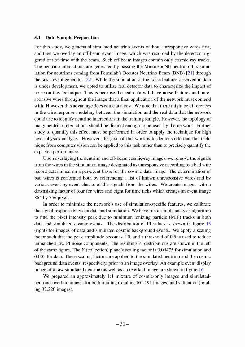
In order to minimize the network’s use of simulation-specific features, we calibratethe signal response between data and simulation. We have run a simple analysis algorithmto find the pixel intensity peak due to minimum ionizing particle (MIP) tracks in bothdata and simulated cosmic events. The distribution of PI values is shown in figure 15(right) for images of data and simulated cosmic background events. We apply a scalingfactor such that the peak amplitude becomes 1.0, and a threshold of 0.5 is used to reduceunmatched low PI noise components. The resulting PI distributions are shown in the leftof the same figure. The Y (collection) plane’s scaling factor is 0.00475 for simulation and0.005 for data. These scaling factors are applied to the simulated neutrino and the cosmicbackground data events, respectively, prior to an image overlay. An example event displayimage of a raw simulated neutrino as well as an overlaid image are shown in figure 16.

We prepared an approximately 1:1 mixture of cosmic-only images and simulated-neutrino-overlaid images for both training (totaling 101,191 images) and validation (total-ing 32,220 images).

– 30 –

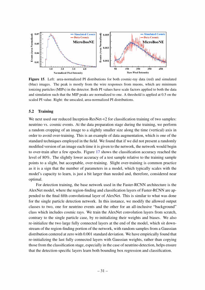
Figure 15. Left: area-normalized PI distributions for both cosmic-ray data (red) and simulated(blue) images. The peak is mostly from the wire responses from muons, which are minimumionizing particles (MIPs) in the detector. Both PI values have scale factors applied to both the dataand simulation such that the MIP peaks are normalized to one. A threshold is applied at 0.5 on thescaled PI value. Right: the unscaled, area-normalized PI distributions.

5.2 Training

We next used our reduced Inception-ResNet-v2 for classification training of two samples:neutrino vs. cosmic events. At the data preparation stage during the training, we performa random cropping of an image to a slightly smaller size along the time (vertical) axis inorder to avoid over-training. This is an example of data augmentation, which is one of thestandard techniques employed in the field. We found that if we did not present a randomlymodified version of an image each time it is given to the network, the network would beginto over-train after a few epochs. Figure 17 shows the classification accuracy reached thelevel of 80%. The slightly lower accuracy of a test sample relative to the training samplepoints to a slight, but acceptable, over-training. Slight over-training is common practiceas it is a sign that the number of parameters in a model, which typically scales with themodel’s capacity to learn, is just a bit larger than needed and, therefore, considered nearoptimal.

For detection training, the base network used in the Faster-RCNN architecture is theAlexNet model, where the region-finding and classification layers of Faster-RCNN are ap-pended to the final fifth convolutional layer of AlexNet. This is similar to what was donefor the single particle detection network. In this instance, we modify the allowed outputclasses to two, one for neutrino events and the other for an all-inclusive “background”class which includes cosmic rays. We train the AlexNet convolution layers from scratch,contrary to the single particle case, by re-initializing their weights and biases. We alsore-initialize the two large fully connected layers at the end of the model, which sit down-stream of the region-finding portion of the network, with random samples from a Gaussiandistribution centered at zero with 0.001 standard deviation. We have empirically found thatre-initializing the last fully connected layers with Gaussian weights, rather than copyingthose from the classification stage, especially in the case of neutrino detection, helps ensurethat the detection-specific layers learn both bounding box regression and classification.

– 31 –

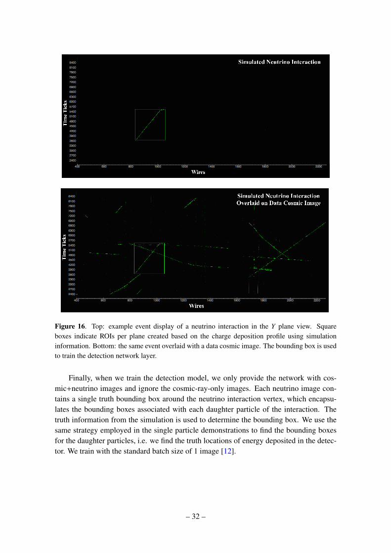
Figure 16. Top: example event display of a neutrino interaction in the Y plane view. Squareboxes indicate ROIs per plane created based on the charge deposition profile using simulationinformation. Bottom: the same event overlaid with a data cosmic image. The bounding box is usedto train the detection network layer.

Finally, when we train the detection model, we only provide the network with cos-mic+neutrino images and ignore the cosmic-ray-only images. Each neutrino image con-tains a single truth bounding box around the neutrino interaction vertex, which encapsu-lates the bounding boxes associated with each daughter particle of the interaction. Thetruth information from the simulation is used to determine the bounding box. We use thesame strategy employed in the single particle demonstrations to find the bounding boxesfor the daughter particles, i.e. we find the truth locations of energy deposited in the detec-tor. We train with the standard batch size of 1 image [12].

– 32 –

0 2 4 6 8 10 12 14 16 18Epoch

0.0

0.2

0.4

0.6

0.8

1.0Loss

Loss vs. Epoch

loss per batch

average loss (100 batch)

0 2 4 6 8 10 12 14 16 18Epoch

0.0

0.2

0.4

0.6

0.8

1.0

Accu

racy

Accuracy vs. Epoch

training accuracy per batch

average training accuracy (100 batch)

test accuracy

Figure 17. Left: 1-plane classification loss curve for our simplified version of Inception-ResNet-v2. Right: accuracy curve monitored during training. In both plots the blue data points are com-puted from the training process while red data points are our interpretation by taking an averageof 100 consecutive blue data points. The magenta curve on the right plot is an accuracy computedusing a test sample.

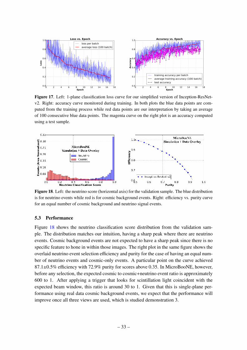
Figure 18. Left: the neutrino score (horizontal axis) for the validation sample. The blue distributionis for neutrino events while red is for cosmic background events. Right: efficiency vs. purity curvefor an equal number of cosmic background and neutrino signal events.

5.3 Performance

Figure 18 shows the neutrino classification score distribution from the validation sam-ple. The distribution matches our intuition, having a sharp peak where there are neutrinoevents. Cosmic background events are not expected to have a sharp peak since there is nospecific feature to hone in within those images. The right plot in the same figure shows theoverlaid neutrino event selection efficiency and purity for the case of having an equal num-ber of neutrino events and cosmic-only events. A particular point on the curve achieved87.1±0.5% efficiency with 72.9% purity for scores above 0.35. In MicroBooNE, however,before any selection, the expected cosmic to cosmic+neutrino event ratio is approximately600 to 1. After applying a trigger that looks for scintillation light coincident with theexpected beam window, this ratio is around 30 to 1. Given that this is single-plane per-formance using real data cosmic background events, we expect that the performance willimprove once all three views are used, which is studied demonstration 3.

– 33 –

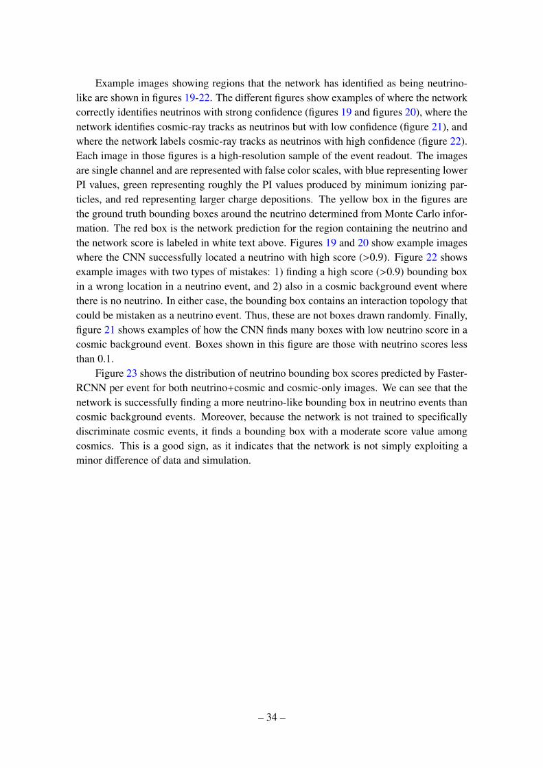
Example images showing regions that the network has identified as being neutrino-like are shown in figures 19-22. The different figures show examples of where the networkcorrectly identifies neutrinos with strong confidence (figures 19 and figures 20), where thenetwork identifies cosmic-ray tracks as neutrinos but with low confidence (figure 21), andwhere the network labels cosmic-ray tracks as neutrinos with high confidence (figure 22).Each image in those figures is a high-resolution sample of the event readout. The imagesare single channel and are represented with false color scales, with blue representing lowerPI values, green representing roughly the PI values produced by minimum ionizing par-ticles, and red representing larger charge depositions. The yellow box in the figures arethe ground truth bounding boxes around the neutrino determined from Monte Carlo infor-mation. The red box is the network prediction for the region containing the neutrino andthe network score is labeled in white text above. Figures 19 and 20 show example imageswhere the CNN successfully located a neutrino with high score (>0.9). Figure 22 showsexample images with two types of mistakes: 1) finding a high score (>0.9) bounding boxin a wrong location in a neutrino event, and 2) also in a cosmic background event wherethere is no neutrino. In either case, the bounding box contains an interaction topology thatcould be mistaken as a neutrino event. Thus, these are not boxes drawn randomly. Finally,figure 21 shows examples of how the CNN finds many boxes with low neutrino score in acosmic background event. Boxes shown in this figure are those with neutrino scores lessthan 0.1.

Figure 23 shows the distribution of neutrino bounding box scores predicted by Faster-RCNN per event for both neutrino+cosmic and cosmic-only images. We can see that thenetwork is successfully finding a more neutrino-like bounding box in neutrino events thancosmic background events. Moreover, because the network is not trained to specificallydiscriminate cosmic events, it finds a bounding box with a moderate score value amongcosmics. This is a good sign, as it indicates that the network is not simply exploiting aminor difference of data and simulation.

– 34 –

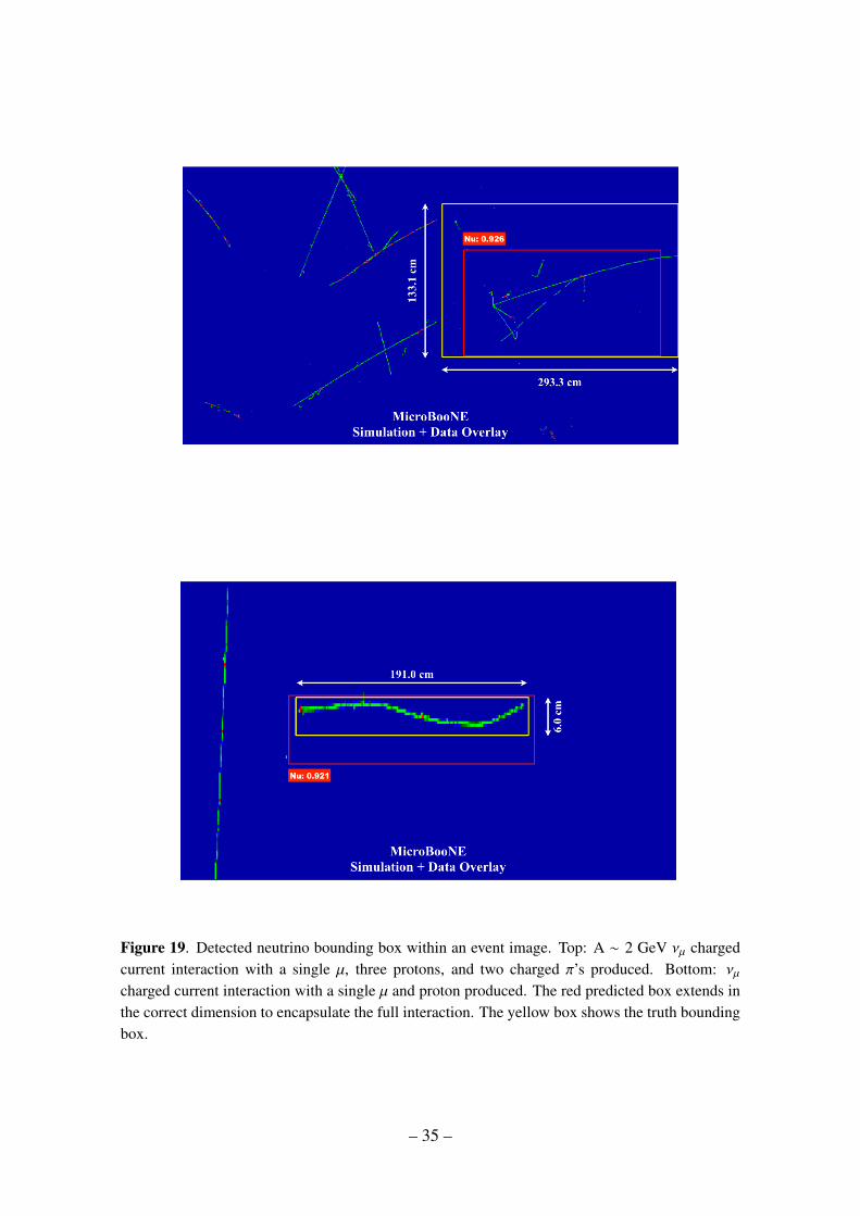
Figure 19. Detected neutrino bounding box within an event image. Top: A ∼ 2 GeV νµ chargedcurrent interaction with a single µ, three protons, and two charged π’s produced. Bottom: νµcharged current interaction with a single µ and proton produced. The red predicted box extends inthe correct dimension to encapsulate the full interaction. The yellow box shows the truth boundingbox.

– 35 –

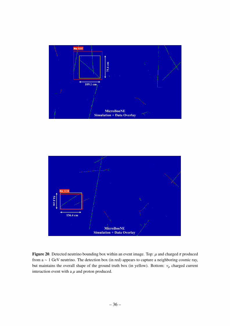
Figure 20. Detected neutrino bounding box within an event image. Top: µ and charged π producedfrom a ∼ 1 GeV neutrino. The detection box (in red) appears to capture a neighboring cosmic ray,but maintains the overall shape of the ground truth box (in yellow). Bottom: νµ charged currentinteraction event with a µ and proton produced.

– 36 –

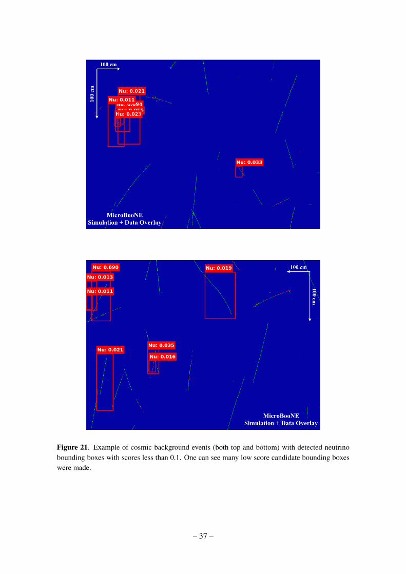
Figure 21. Example of cosmic background events (both top and bottom) with detected neutrinobounding boxes with scores less than 0.1. One can see many low score candidate bounding boxeswere made.

– 37 –

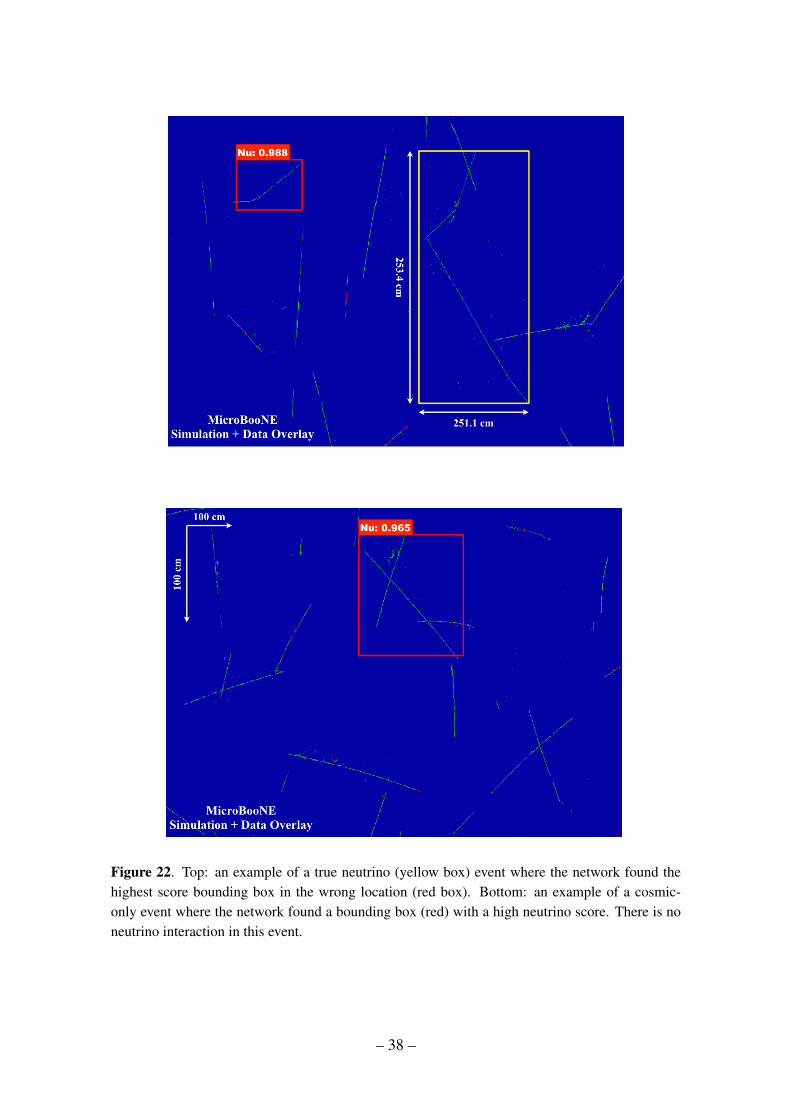
Figure 22. Top: an example of a true neutrino (yellow box) event where the network found thehighest score bounding box in the wrong location (red box). Bottom: an example of a cosmic-only event where the network found a bounding box (red) with a high neutrino score. There is noneutrino interaction in this event.

– 38 –

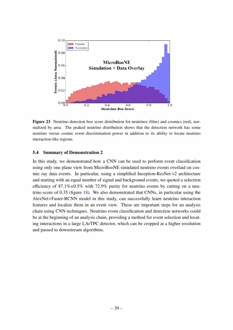
Figure 23. Neutrino detection box score distribution for neutrinos (blue) and cosmics (red), nor-malized by area. The peaked neutrino distribution shows that the detection network has someneutrino versus cosmic event discrimination power in addition to its ability to locate neutrinointeraction-like regions.

5.4 Summary of Demonstration 2

In this study, we demonstrated how a CNN can be used to perform event classificationusing only one plane view from MicroBooNE simulated neutrino events overlaid on cos-mic ray data events. In particular, using a simplified Inception-ResNet-v2 architectureand starting with an equal number of signal and background events, we quoted a selectionefficiency of 87.1%±0.5% with 72.9% purity for neutrino events by cutting on a neu-trino score of 0.35 (figure 18). We also demonstrated that CNNs, in particular using theAlexNet+Faster-RCNN model in this study, can successfully learn neutrino interactionfeatures and localize them in an event view. These are important steps for an analysischain using CNN techniques. Neutrino event classification and detection networks couldbe at the beginning of an analysis chain, providing a method for event selection and locat-ing interactions in a large LArTPC detector, which can be cropped at a higher resolutionand passed to downstream algorithms.

– 39 –

6 Demonstration 3: Neutrino Event Identification with 3 Planes andOptical Detector

In this section, we report on the study of neutrino event classification using the full Micro-BooNE detector information including TPC three-plane data in combination with opticaldetector data. We employ a novel network architecture based on ResNet [14] with a dataaugmentation technique for combining TPC and optical detector data in an event image.We first describe sample preparation and network training methods. The general strategyof using a simulated neutrino image overlaid on a cosmic background image taken fromdata stays the same as in the previous demonstration.

6.1 Network Design

The network we designed for the three-plane neutrino classification task is based on theResNet network [14]. This network features the repeated use of what are referred to asresidual convolutional modules. These modules have been demonstrated to help networkstrain more quickly [13]. As described in more detail below, the input images are chosen tobe 768×768 pixels with 12 channels as a third dimension. This is a relatively large amountof input data for a network compared to existing models. This compelled us to employ anetwork model based on a truncated ResNet network. This constraint arises because of thememory limitation of the GPUs, which is 12 GB. The more slowly one reduces the size ofthe output feature maps at each layer, the more memory that is required at each given layer.This means that there can be fewer layers and that each layer can learn fewer filters. Morelayers and filters mean that the network can learn more and, in principle, attain a higherperformance. However, by preserving the resolution of the feature maps, the network isexposed to more detailed features in the image. Fully exploring the space of the networkconfigurations is reserved for future studies.

The full neutrino ID network shown in figure 24 uses all three TPC planes. The threeplanes are passed separately through the stem portion of the network which consists ofthree convolutional layers, along with a couple of pooling layers to reduce the size ofthe output feature map. All convolutional layers (in both the stem and elsewhere) usea technique known as batch normalization [23] and are followed by a ReLU. Note thatthe convolutional layers in the stem are the same for all three views. In other words,the parameters of those layers are shared. The output feature maps of the stem are thenconcatenated and passed through nine residual modules. This is followed by an averagepooling layer that incorporates a technique known as dropout [24]. After the dropoutlayer, two fully-connected layers are used to classify the output features and determine ifthe event has a neutrino or not. For more details on the network and different componentlayers included please see appendix A.

– 40 –

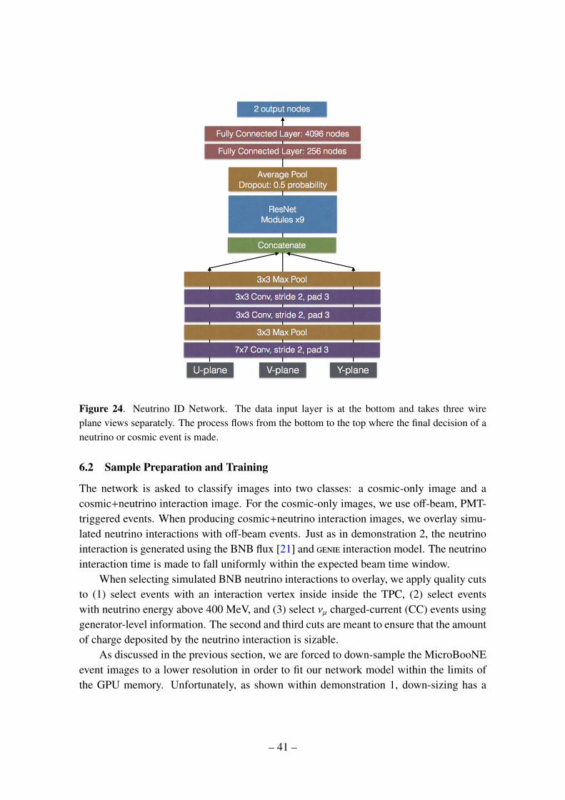
Figure 24. Neutrino ID Network. The data input layer is at the bottom and takes three wireplane views separately. The process flows from the bottom to the top where the final decision of aneutrino or cosmic event is made.

6.2 Sample Preparation and Training

The network is asked to classify images into two classes: a cosmic-only image and acosmic+neutrino interaction image. For the cosmic-only images, we use off-beam, PMT-triggered events. When producing cosmic+neutrino interaction images, we overlay simu-lated neutrino interactions with off-beam events. Just as in demonstration 2, the neutrinointeraction is generated using the BNB flux [21] and genie interaction model. The neutrinointeraction time is made to fall uniformly within the expected beam time window.

When selecting simulated BNB neutrino interactions to overlay, we apply quality cutsto (1) select events with an interaction vertex inside inside the TPC, (2) select eventswith neutrino energy above 400 MeV, and (3) select νµ charged-current (CC) events usinggenerator-level information. The second and third cuts are meant to ensure that the amountof charge deposited by the neutrino interaction is sizable.

As discussed in the previous section, we are forced to down-sample the MicroBooNEevent images to a lower resolution in order to fit our network model within the limits ofthe GPU memory. Unfortunately, as shown within demonstration 1, down-sizing has a

– 41 –

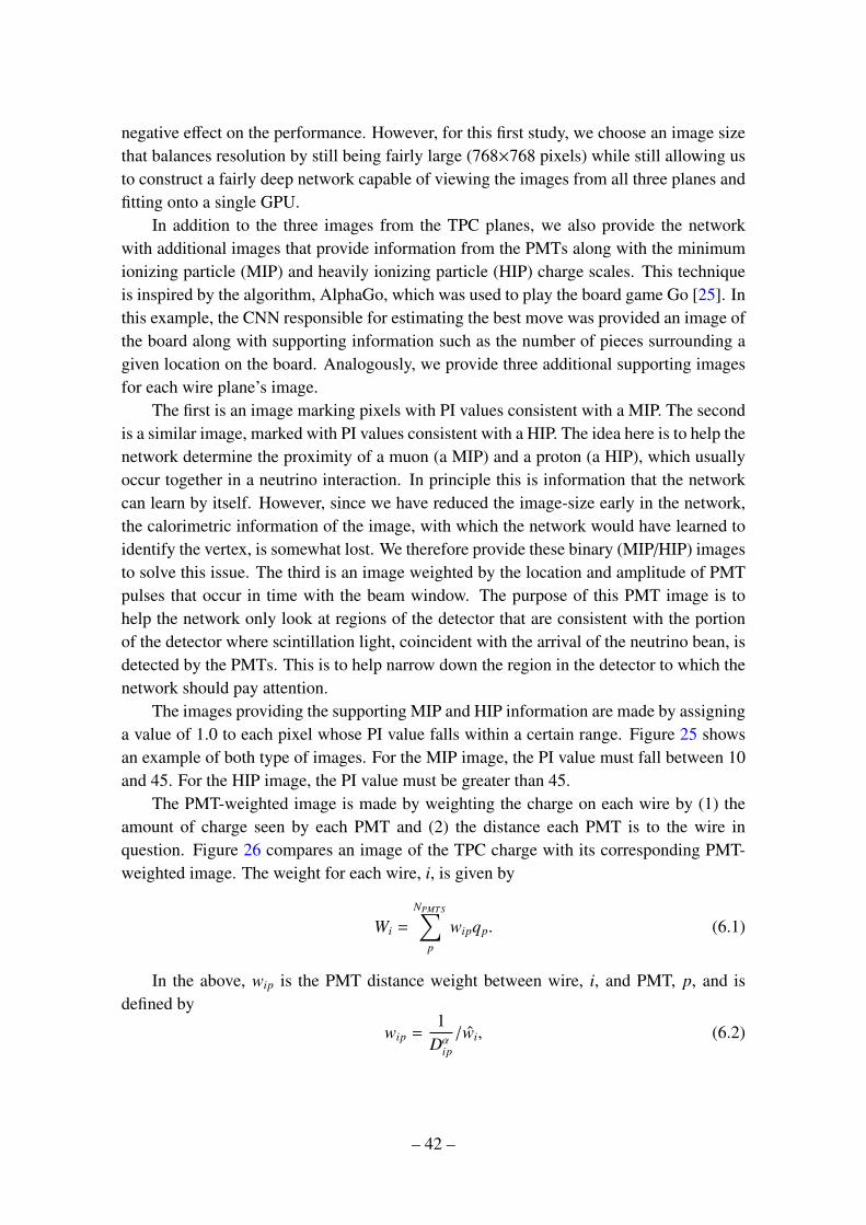
negative effect on the performance. However, for this first study, we choose an image sizethat balances resolution by still being fairly large (768×768 pixels) while still allowing usto construct a fairly deep network capable of viewing the images from all three planes andfitting onto a single GPU.

In addition to the three images from the TPC planes, we also provide the networkwith additional images that provide information from the PMTs along with the minimumionizing particle (MIP) and heavily ionizing particle (HIP) charge scales. This techniqueis inspired by the algorithm, AlphaGo, which was used to play the board game Go [25]. Inthis example, the CNN responsible for estimating the best move was provided an image ofthe board along with supporting information such as the number of pieces surrounding agiven location on the board. Analogously, we provide three additional supporting imagesfor each wire plane’s image.

The first is an image marking pixels with PI values consistent with a MIP. The secondis a similar image, marked with PI values consistent with a HIP. The idea here is to help thenetwork determine the proximity of a muon (a MIP) and a proton (a HIP), which usuallyoccur together in a neutrino interaction. In principle this is information that the networkcan learn by itself. However, since we have reduced the image-size early in the network,the calorimetric information of the image, with which the network would have learned toidentify the vertex, is somewhat lost. We therefore provide these binary (MIP/HIP) imagesto solve this issue. The third is an image weighted by the location and amplitude of PMTpulses that occur in time with the beam window. The purpose of this PMT image is tohelp the network only look at regions of the detector that are consistent with the portionof the detector where scintillation light, coincident with the arrival of the neutrino bean, isdetected by the PMTs. This is to help narrow down the region in the detector to which thenetwork should pay attention.

The images providing the supporting MIP and HIP information are made by assigninga value of 1.0 to each pixel whose PI value falls within a certain range. Figure 25 showsan example of both type of images. For the MIP image, the PI value must fall between 10and 45. For the HIP image, the PI value must be greater than 45.

The PMT-weighted image is made by weighting the charge on each wire by (1) theamount of charge seen by each PMT and (2) the distance each PMT is to the wire inquestion. Figure 26 compares an image of the TPC charge with its corresponding PMT-weighted image. The weight for each wire, i, is given by

Wi =

NPMTS∑p

wipqp. (6.1)

In the above, wip is the PMT distance weight between wire, i, and PMT, p, and isdefined by

wip =1

Dαip/wi, (6.2)

– 42 –

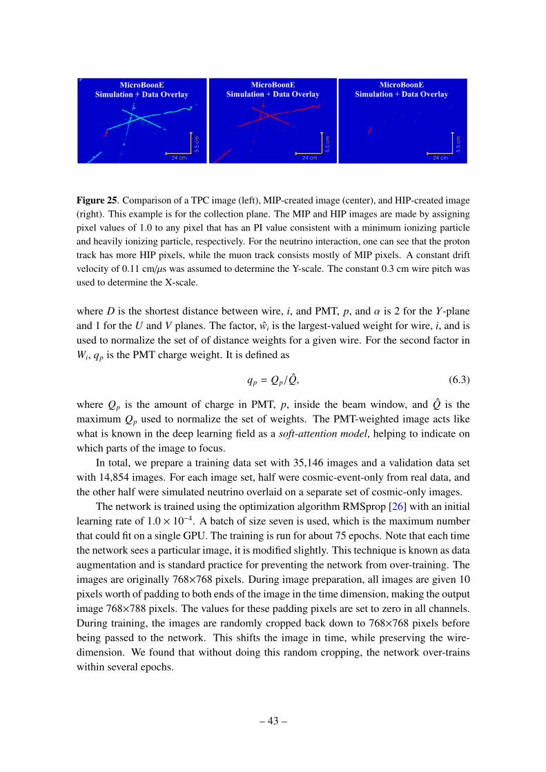
5.5

cm

24 cm

5.5

cm

24 cm

5.5

cm

24 cm

Figure 25. Comparison of a TPC image (left), MIP-created image (center), and HIP-created image(right). This example is for the collection plane. The MIP and HIP images are made by assigningpixel values of 1.0 to any pixel that has an PI value consistent with a minimum ionizing particleand heavily ionizing particle, respectively. For the neutrino interaction, one can see that the protontrack has more HIP pixels, while the muon track consists mostly of MIP pixels. A constant driftvelocity of 0.11 cm/µs was assumed to determine the Y-scale. The constant 0.3 cm wire pitch wasused to determine the X-scale.

where D is the shortest distance between wire, i, and PMT, p, and α is 2 for the Y-planeand 1 for the U and V planes. The factor, wi is the largest-valued weight for wire, i, and isused to normalize the set of of distance weights for a given wire. For the second factor inWi, qp is the PMT charge weight. It is defined as

qp = Qp/Q, (6.3)

where Qp is the amount of charge in PMT, p, inside the beam window, and Q is themaximum Qp used to normalize the set of weights. The PMT-weighted image acts likewhat is known in the deep learning field as a soft-attention model, helping to indicate onwhich parts of the image to focus.

In total, we prepare a training data set with 35,146 images and a validation data setwith 14,854 images. For each image set, half were cosmic-event-only from real data, andthe other half were simulated neutrino overlaid on a separate set of cosmic-only images.

The network is trained using the optimization algorithm RMSprop [26] with an initiallearning rate of 1.0 × 10−4. A batch of size seven is used, which is the maximum numberthat could fit on a single GPU. The training is run for about 75 epochs. Note that each timethe network sees a particular image, it is modified slightly. This technique is known as dataaugmentation and is standard practice for preventing the network from over-training. Theimages are originally 768×768 pixels. During image preparation, all images are given 10pixels worth of padding to both ends of the image in the time dimension, making the outputimage 768×788 pixels. The values for these padding pixels are set to zero in all channels.During training, the images are randomly cropped back down to 768×768 pixels beforebeing passed to the network. This shifts the image in time, while preserving the wire-dimension. We found that without doing this random cropping, the network over-trainswithin several epochs.

– 43 –

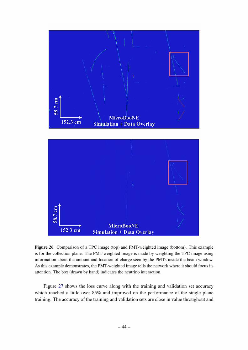
Figure 26. Comparison of a TPC image (top) and PMT-weighted image (bottom). This exampleis for the collection plane. The PMT-weighted image is made by weighting the TPC image usinginformation about the amount and location of charge seen by the PMTs inside the beam window.As this example demonstrates, the PMT-weighted image tells the network where it should focus itsattention. The box (drawn by hand) indicates the neutrino interaction.

Figure 27 shows the loss curve along with the training and validation set accuracywhich reached a little over 85% and improved on the performance of the single planetraining. The accuracy of the training and validation sets are close in value throughout and

– 44 –

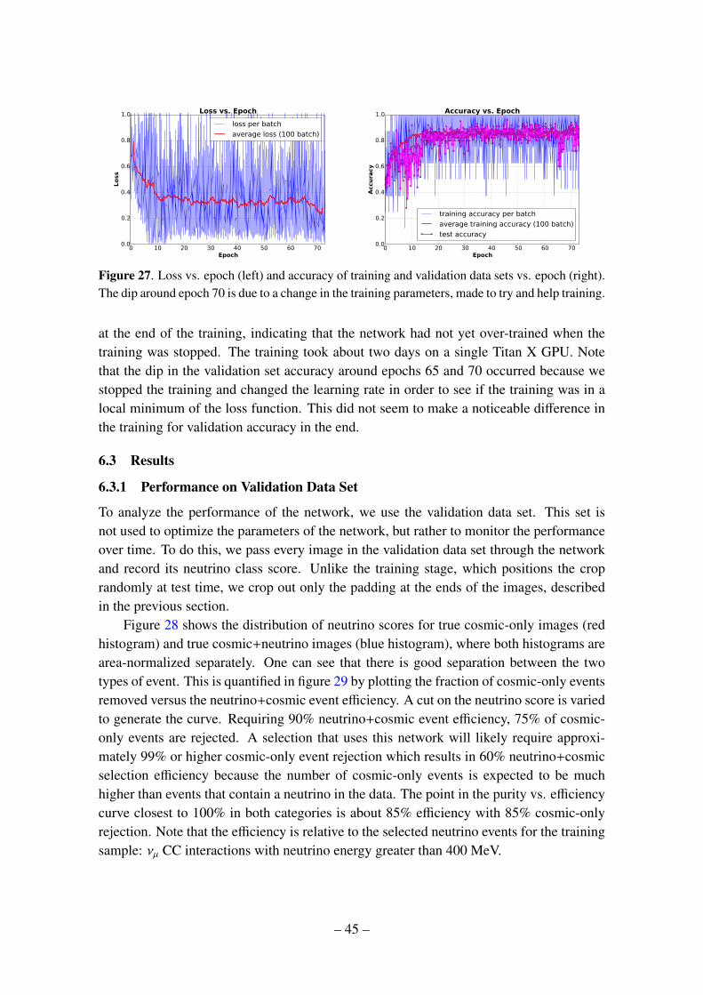
0 10 20 30 40 50 60 70Epoch

0.0

0.2

0.4

0.6

0.8

1.0Loss

Loss vs. Epoch

loss per batch

average loss (100 batch)

0 10 20 30 40 50 60 70Epoch

0.0

0.2

0.4

0.6

0.8

1.0

Accu

racy

Accuracy vs. Epoch

training accuracy per batch

average training accuracy (100 batch)

test accuracy

Figure 27. Loss vs. epoch (left) and accuracy of training and validation data sets vs. epoch (right).The dip around epoch 70 is due to a change in the training parameters, made to try and help training.

at the end of the training, indicating that the network had not yet over-trained when thetraining was stopped. The training took about two days on a single Titan X GPU. Notethat the dip in the validation set accuracy around epochs 65 and 70 occurred because westopped the training and changed the learning rate in order to see if the training was in alocal minimum of the loss function. This did not seem to make a noticeable difference inthe training for validation accuracy in the end.

6.3 Results

6.3.1 Performance on Validation Data Set

To analyze the performance of the network, we use the validation data set. This set isnot used to optimize the parameters of the network, but rather to monitor the performanceover time. To do this, we pass every image in the validation data set through the networkand record its neutrino class score. Unlike the training stage, which positions the croprandomly at test time, we crop out only the padding at the ends of the images, describedin the previous section.

Figure 28 shows the distribution of neutrino scores for true cosmic-only images (redhistogram) and true cosmic+neutrino images (blue histogram), where both histograms arearea-normalized separately. One can see that there is good separation between the twotypes of event. This is quantified in figure 29 by plotting the fraction of cosmic-only eventsremoved versus the neutrino+cosmic event efficiency. A cut on the neutrino score is variedto generate the curve. Requiring 90% neutrino+cosmic event efficiency, 75% of cosmic-only events are rejected. A selection that uses this network will likely require approxi-mately 99% or higher cosmic-only event rejection which results in 60% neutrino+cosmicselection efficiency because the number of cosmic-only events is expected to be muchhigher than events that contain a neutrino in the data. The point in the purity vs. efficiencycurve closest to 100% in both categories is about 85% efficiency with 85% cosmic-onlyrejection. Note that the efficiency is relative to the selected neutrino events for the trainingsample: νµ CC interactions with neutrino energy greater than 400 MeV.

– 45 –

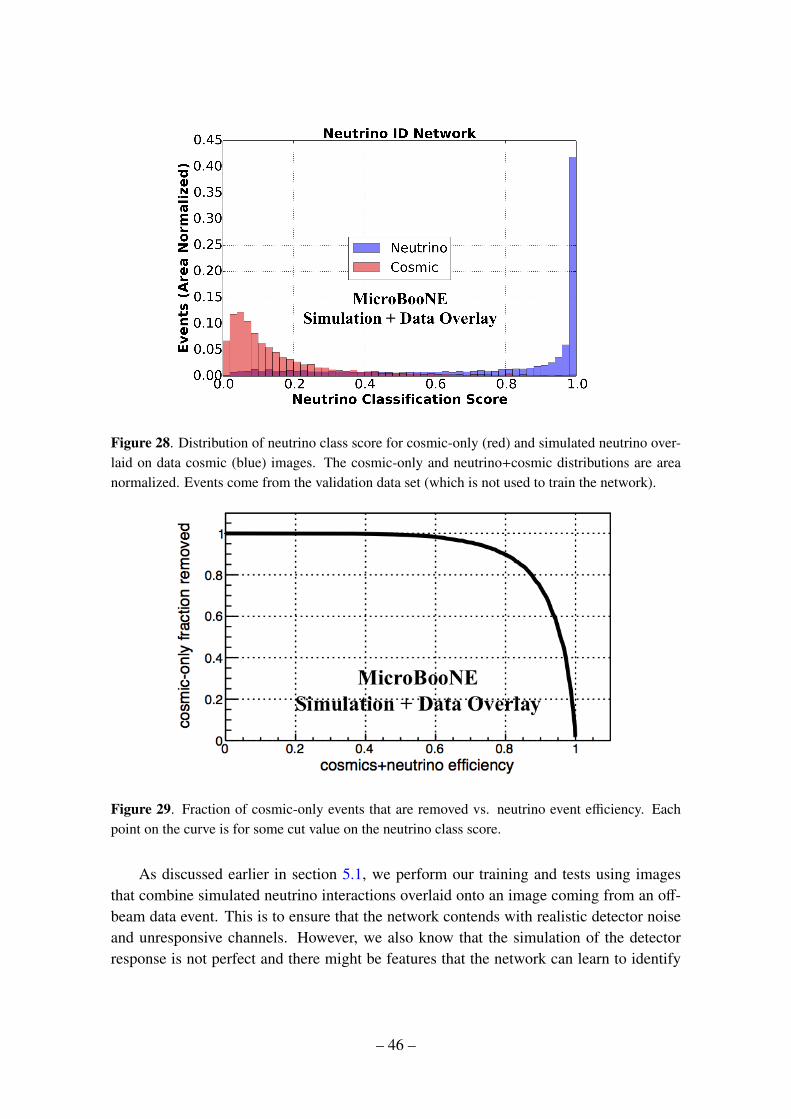
Figure 28. Distribution of neutrino class score for cosmic-only (red) and simulated neutrino over-laid on data cosmic (blue) images. The cosmic-only and neutrino+cosmic distributions are areanormalized. Events come from the validation data set (which is not used to train the network).

Figure 29. Fraction of cosmic-only events that are removed vs. neutrino event efficiency. Eachpoint on the curve is for some cut value on the neutrino class score.

As discussed earlier in section 5.1, we perform our training and tests using imagesthat combine simulated neutrino interactions overlaid onto an image coming from an off-beam data event. This is to ensure that the network contends with realistic detector noiseand unresponsive channels. However, we also know that the simulation of the detectorresponse is not perfect and there might be features that the network can learn to identify

– 46 –

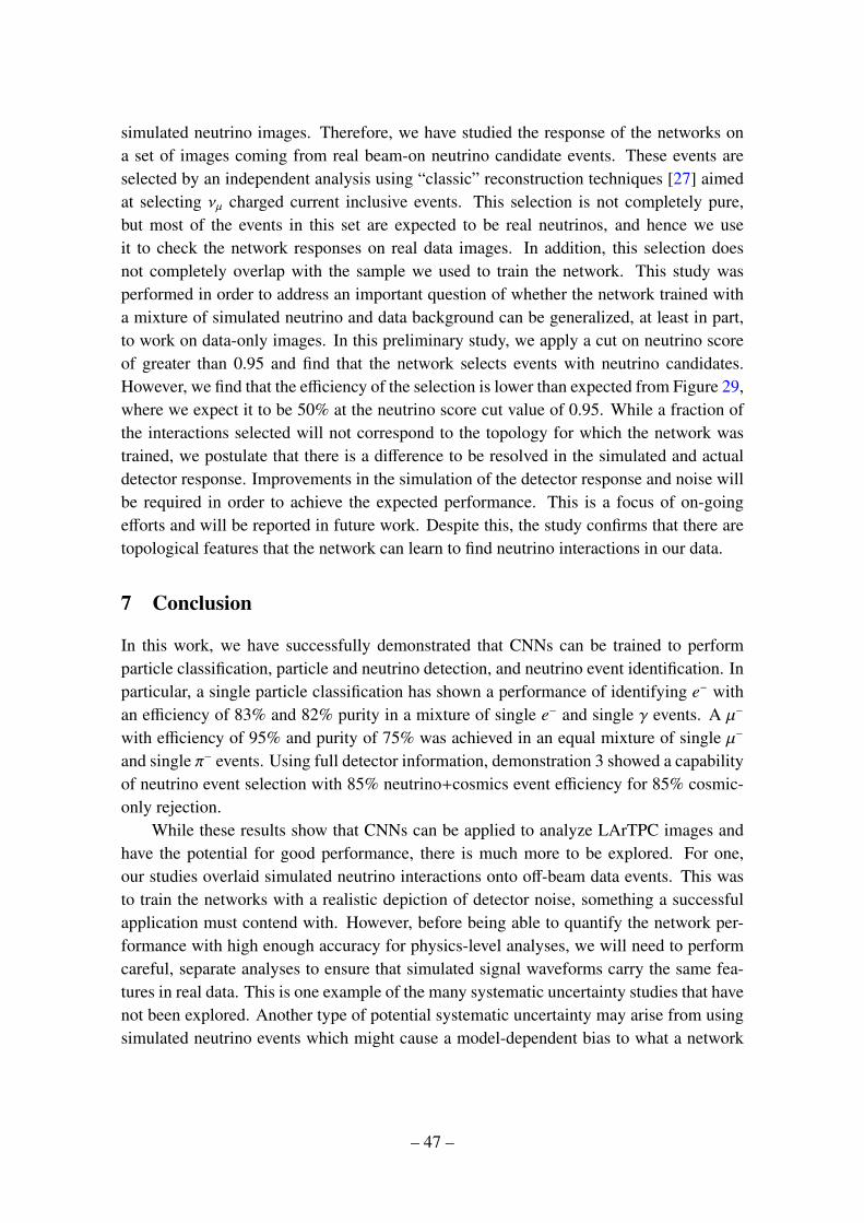
simulated neutrino images. Therefore, we have studied the response of the networks ona set of images coming from real beam-on neutrino candidate events. These events areselected by an independent analysis using “classic” reconstruction techniques [27] aimedat selecting νµ charged current inclusive events. This selection is not completely pure,but most of the events in this set are expected to be real neutrinos, and hence we useit to check the network responses on real data images. In addition, this selection doesnot completely overlap with the sample we used to train the network. This study wasperformed in order to address an important question of whether the network trained witha mixture of simulated neutrino and data background can be generalized, at least in part,to work on data-only images. In this preliminary study, we apply a cut on neutrino scoreof greater than 0.95 and find that the network selects events with neutrino candidates.However, we find that the efficiency of the selection is lower than expected from Figure 29,where we expect it to be 50% at the neutrino score cut value of 0.95. While a fraction ofthe interactions selected will not correspond to the topology for which the network wastrained, we postulate that there is a difference to be resolved in the simulated and actualdetector response. Improvements in the simulation of the detector response and noise willbe required in order to achieve the expected performance. This is a focus of on-goingefforts and will be reported in future work. Despite this, the study confirms that there aretopological features that the network can learn to find neutrino interactions in our data.

7 Conclusion

In this work, we have successfully demonstrated that CNNs can be trained to performparticle classification, particle and neutrino detection, and neutrino event identification. Inparticular, a single particle classification has shown a performance of identifying e− withan efficiency of 83% and 82% purity in a mixture of single e− and single γ events. A µ−

with efficiency of 95% and purity of 75% was achieved in an equal mixture of single µ−

and single π− events. Using full detector information, demonstration 3 showed a capabilityof neutrino event selection with 85% neutrino+cosmics event efficiency for 85% cosmic-only rejection.

While these results show that CNNs can be applied to analyze LArTPC images andhave the potential for good performance, there is much more to be explored. For one,our studies overlaid simulated neutrino interactions onto off-beam data events. This wasto train the networks with a realistic depiction of detector noise, something a successfulapplication must contend with. However, before being able to quantify the network per-formance with high enough accuracy for physics-level analyses, we will need to performcareful, separate analyses to ensure that simulated signal waveforms carry the same fea-tures in real data. This is one example of the many systematic uncertainty studies that havenot been explored. Another type of potential systematic uncertainty may arise from usingsimulated neutrino events which might cause a model-dependent bias to what a network

– 47 –

learns. Careful study is required to quantify the bias, and to minimize it wherever possi-ble. Alternatively, one might instead develop a model-independent approach for detectingneutrinos in data. Such studies are a requirement for physics analyses using this techniqueand developing new methods to quantify this will be explored in future work.

Overall, this work takes the first steps in exploring CNNs and the broader disciplineof the field of deep learning, a collective term for algorithms and architectures that employdeep neural networks, to LArTPCs. We have shown the following:

• It is necessary to consider a strategy to either crop or downsize images for a largeLArTPC detector, and study their effect. We have shown one possible method(demonstration 1).

• As long as GPU memory constraints are not an issue, it is best to limit downsizing asthe networks use dE/dx information for classification. A downsizing of the imagesby a factor of 2 showed a clear negative effect (demonstration 1).

• For a particle classification task, using weights for a network trained for a greatervariety of features might perform better. This was seen in the µ−/π− study, wherethe network trained for five-particle classification outperformed the same networktrained for only the µ−/π− sample (demonstration 1).

• The Faster-RCNN architecture can be used for neutrino interaction detection in alarge event image (demonstration 2).

• It is possible to combine different types of detector information to enhance the fea-tures in the image data. We have shown one method to combine PMT and TPCinformation as an illustration (demonstration 3).

• A multi-view architecture can be employed to process multiple TPC plane-views forneutrino interaction selection, and to enhance the performance achieved comparedto using single plane information only (demonstration 3).

• Modeling of the wire response and noise characteristics of the detector need im-provement before a network trained on simulated images can be fully generalized toreal data images. Likewise, techniques to mitigate the impact of this disagreementshould be developed.

There are certainly many other avenues, besides the ones listed here, to study and possiblyimprove performance. However, the proof-of-principle tests conducted in this work showthat CNNs can deliver results worthy of further exploration and provide a useful starting-point for those interested in developing their own CNNs for the reconstruction of neutrinoevents in liquid argon TPCs.

– 48 –

Acknowledgments

This material is based upon work supported by the following: the U.S. Department ofEnergy, Office of Science, Offices of High Energy Physics and Nuclear Physics; the U.S.National Science Foundation; the Swiss National Science Foundation; the Science andTechnology Facilities Council of the United Kingdom; and The Royal Society (UnitedKingdom). Additional support for the laser calibration system and cosmic ray tagger wasprovided by the Albert Einstein Center for Fundamental Physics. Fermilab is operatedby Fermi Research Alliance, LLC under Contract No. DE-AC02-07CH11359 with theUnited States Department of Energy.

– 49 –

A Details of the Components in the Three-plane Neutrino ID Net-work

This appendix provides more details of some of the techniques incorporated into the net-work described in section 6.1.

The primary type of network layer employed is known as the residual convolutionalmodule [14]. The basic idea is that instead of training the network to optimize a func-tion, F(x), over the feature space, x, it is easier for a network to optimize residuals, H(x),such that F(x) = x + H(x). A diagram of the residual module employed in our networkis given in figure 30. The insight of the authors of ref [14] arose from their experiencein training very deep networks where the number of layers surpasses 100 or more. Whatthey found is that these very deep networks perform worse than shallower ones. Thisseemed counter-intuitive, because if additional layers were not useful, a network in princi-ple should just learn to use the identity convolution to pass existing feature maps forwardin the network and retain the same performance, all things being equal. This insight ledthem to hypothesize that with deep networks it was difficult (or just required too muchtime) for convolutional layers to optimize to the identity if it needed. Therefore, the resid-ual module, which can be initialized near H(x) ≈ 0, allows a layer to start at the identityconvolution and optimize from there.

Another proposed reason this network structure is useful is that during training theamount of error made by the network can back-propagate more easily through the network.As can be seen in figure 30, information passing backwards can flow both through theconvolutional layers and through a so-called bypass connection directly back to the inputfeature map. The bypass protects the information from potentially small derivative valuescoming from the convolutional layers. Other studies showed that non-residual, very deepnetworks, while they do not necessarily perform worse than residual networks, train moreslowly than residual networks [13]. That residual networks train faster corroborates bothhypotheses as to why residual network structures are effective and, thereby, more thanwarrant their use. Based on these findings, we use these types of modules in the networkof demonstration 3 above.

Our version of the residual module follows that used in ref. [14]. We use a 3×3convolution that is both preceded and followed by 1×1 convolutions. The output of eachconvolutional layer is passed through a ReLU. It is believed that this (1 × 1) − (3 × 3) −(1 × 1) structure has about the same complexity as two 3×3 convolutions but containsmore non-linearities and fewer free parameters. This is desirable as it is hypothesized toincrease the separation power while reducing over-fitting. The convolutional layers alsouse a technique known as batch normalization, or BatchNorm [23].

BatchNorm is a technique where, for a batch during training, the activation of a layeris normalized to have a mean of zero and a variance of one. This technique is believed toreduce learning time by preventing the distribution of activations of each layer to change,something the authors in ref. [23] refer to as internal covariance shift. BatchNorm also

– 50 –

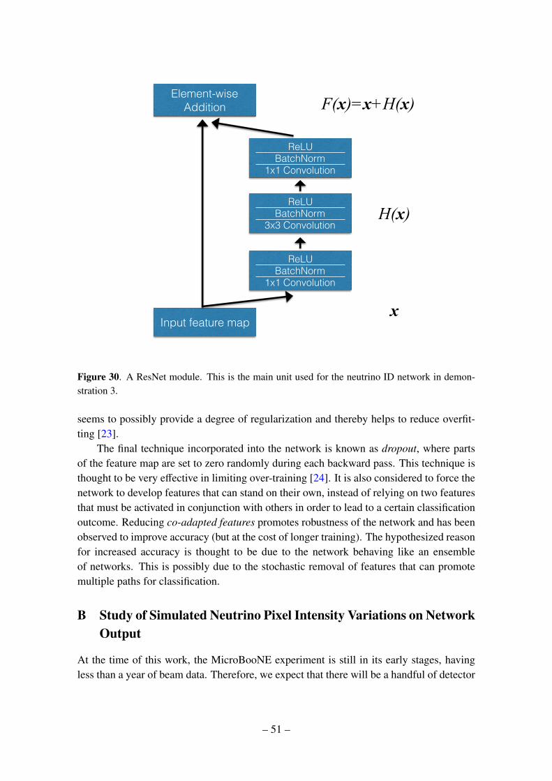
Input feature map

Element-wise Addition

H(x)

x

F(x)=x+H(x)

ReLU BatchNorm

1x1 Convolution

ReLU BatchNorm

3x3 Convolution

ReLU BatchNorm

1x1 Convolution

Figure 30. A ResNet module. This is the main unit used for the neutrino ID network in demon-stration 3.

seems to possibly provide a degree of regularization and thereby helps to reduce overfit-ting [23].

The final technique incorporated into the network is known as dropout, where partsof the feature map are set to zero randomly during each backward pass. This technique isthought to be very effective in limiting over-training [24]. It is also considered to force thenetwork to develop features that can stand on their own, instead of relying on two featuresthat must be activated in conjunction with others in order to lead to a certain classificationoutcome. Reducing co-adapted features promotes robustness of the network and has beenobserved to improve accuracy (but at the cost of longer training). The hypothesized reasonfor increased accuracy is thought to be due to the network behaving like an ensembleof networks. This is possibly due to the stochastic removal of features that can promotemultiple paths for classification.

B Study of Simulated Neutrino Pixel Intensity Variations on NetworkOutput

At the time of this work, the MicroBooNE experiment is still in its early stages, havingless than a year of beam data. Therefore, we expect that there will be a handful of detector

– 51 –

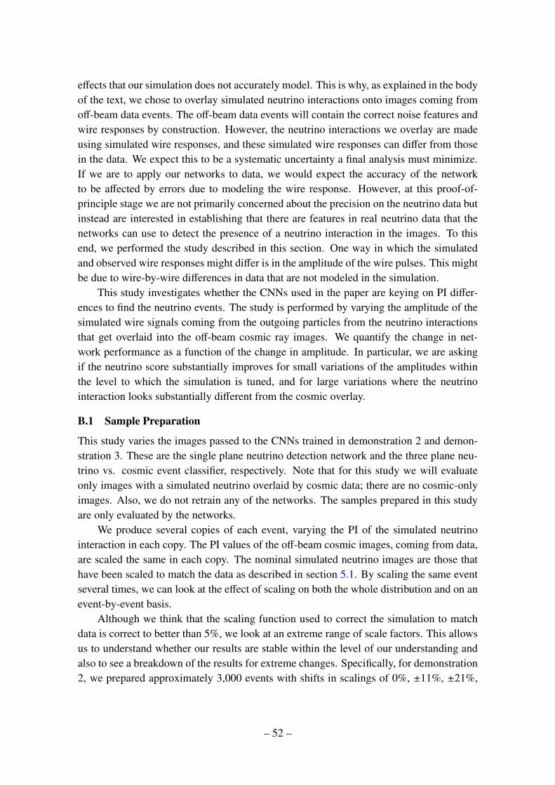
effects that our simulation does not accurately model. This is why, as explained in the bodyof the text, we chose to overlay simulated neutrino interactions onto images coming fromoff-beam data events. The off-beam data events will contain the correct noise features andwire responses by construction. However, the neutrino interactions we overlay are madeusing simulated wire responses, and these simulated wire responses can differ from thosein the data. We expect this to be a systematic uncertainty a final analysis must minimize.If we are to apply our networks to data, we would expect the accuracy of the networkto be affected by errors due to modeling the wire response. However, at this proof-of-principle stage we are not primarily concerned about the precision on the neutrino data butinstead are interested in establishing that there are features in real neutrino data that thenetworks can use to detect the presence of a neutrino interaction in the images. To thisend, we performed the study described in this section. One way in which the simulatedand observed wire responses might differ is in the amplitude of the wire pulses. This mightbe due to wire-by-wire differences in data that are not modeled in the simulation.

This study investigates whether the CNNs used in the paper are keying on PI differ-ences to find the neutrino events. The study is performed by varying the amplitude of thesimulated wire signals coming from the outgoing particles from the neutrino interactionsthat get overlaid into the off-beam cosmic ray images. We quantify the change in net-work performance as a function of the change in amplitude. In particular, we are askingif the neutrino score substantially improves for small variations of the amplitudes withinthe level to which the simulation is tuned, and for large variations where the neutrinointeraction looks substantially different from the cosmic overlay.

B.1 Sample Preparation

This study varies the images passed to the CNNs trained in demonstration 2 and demon-stration 3. These are the single plane neutrino detection network and the three plane neu-trino vs. cosmic event classifier, respectively. Note that for this study we will evaluateonly images with a simulated neutrino overlaid by cosmic data; there are no cosmic-onlyimages. Also, we do not retrain any of the networks. The samples prepared in this studyare only evaluated by the networks.

We produce several copies of each event, varying the PI of the simulated neutrinointeraction in each copy. The PI values of the off-beam cosmic images, coming from data,are scaled the same in each copy. The nominal simulated neutrino images are those thathave been scaled to match the data as described in section 5.1. By scaling the same eventseveral times, we can look at the effect of scaling on both the whole distribution and on anevent-by-event basis.

Although we think that the scaling function used to correct the simulation to matchdata is correct to better than 5%, we look at an extreme range of scale factors. This allowsus to understand whether our results are stable within the level of our understanding andalso to see a breakdown of the results for extreme changes. Specifically, for demonstration2, we prepared approximately 3,000 events with shifts in scalings of 0%, ±11%, ±21%,

– 52 –

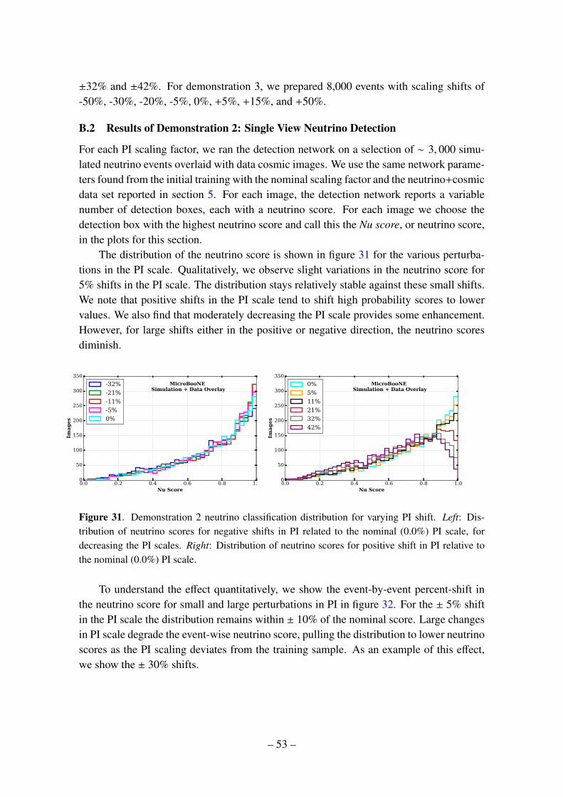
±32% and ±42%. For demonstration 3, we prepared 8,000 events with scaling shifts of-50%, -30%, -20%, -5%, 0%, +5%, +15%, and +50%.

B.2 Results of Demonstration 2: Single View Neutrino Detection

For each PI scaling factor, we ran the detection network on a selection of ∼ 3, 000 simu-lated neutrino events overlaid with data cosmic images. We use the same network parame-ters found from the initial training with the nominal scaling factor and the neutrino+cosmicdata set reported in section 5. For each image, the detection network reports a variablenumber of detection boxes, each with a neutrino score. For each image we choose thedetection box with the highest neutrino score and call this the Nu score, or neutrino score,in the plots for this section.

The distribution of the neutrino score is shown in figure 31 for the various perturba-tions in the PI scale. Qualitatively, we observe slight variations in the neutrino score for5% shifts in the PI scale. The distribution stays relatively stable against these small shifts.We note that positive shifts in the PI scale tend to shift high probability scores to lowervalues. We also find that moderately decreasing the PI scale provides some enhancement.However, for large shifts either in the positive or negative direction, the neutrino scoresdiminish.

0.0 0.2 0.4 0.6 0.8 1.0Nu Score

0

50

100

150

200

250

300

350

Imag

es

MicroBooNE Simulation + Data Overlay

-32%

-21%

-11%

-5%

0%

0.0 0.2 0.4 0.6 0.8 1.0Nu Score

0

50

100

150

200

250

300

350

Imag

es


0%

5%

11%

21%

32%

42%

Figure 31. Demonstration 2 neutrino classification distribution for varying PI shift. Left: Dis-tribution of neutrino scores for negative shifts in PI related to the nominal (0.0%) PI scale, fordecreasing the PI scales. Right: Distribution of neutrino scores for positive shift in PI relative tothe nominal (0.0%) PI scale.

To understand the effect quantitatively, we show the event-by-event percent-shift inthe neutrino score for small and large perturbations in PI in figure 32. For the ± 5% shiftin the PI scale the distribution remains within ± 10% of the nominal score. Large changesin PI scale degrade the event-wise neutrino score, pulling the distribution to lower neutrinoscores as the PI scaling deviates from the training sample. As an example of this effect,we show the ± 30% shifts.

– 53 –

Figure 32. Demonstration 2 event-by-event shift in neutrino score. The blue, and red distributionsare positive and negative PI scalings respectively. Left: Distribution of percent shift in neutrinoscore for smallest perturbation in PI scale. At least 50% of events show less than 1% deviation inneutrino score. Right: Distribution of percent shift in neutrino score for the largest perturbation inPI scale.

The total fraction of events which shift in network probability by a fixed percentage ormore is shown in figure 33. For small (±5%) PI re-scalings, fewer than 10% of the eventsor the events change the network score by an amount of ≥ 10% (red curve). If we make amore stringent test, examining score-changes of ≥ 5%, more than 80% of the event scoresremain stable at or below this level.

If the network were relying on PI scale differences to identify neutrino events withinthe overlaid image, we would have expected much larger instabilities for small perturba-tions. This gives us confidence that the network is relying on other features, such as thepresence of a vertex, to identify neutrino events, and not substantially relying on PI scaledifferences between data and simulation to make its network prediction.

– 54 –

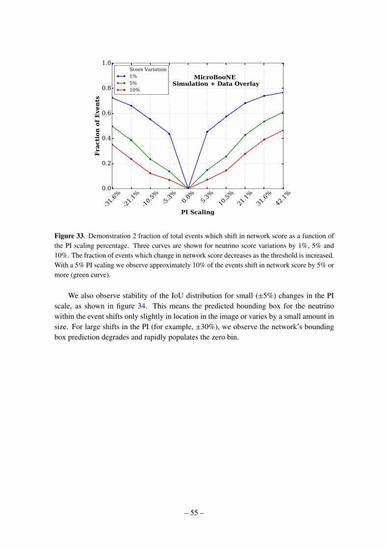
-31.

6%

-21.

1%

-10.

5%-5

.3%

0.0%

5.3%

10.5

%

21.1

%

31.6

%

42.1

%

PI Scaling

0.0

0.2

0.4

0.6

0.8

1.0

Fra

cti

on

of

Eve

nts


Score Variation

1%

5%

10%

Figure 33. Demonstration 2 fraction of total events which shift in network score as a function ofthe PI scaling percentage. Three curves are shown for neutrino score variations by 1%, 5% and10%. The fraction of events which change in network score decreases as the threshold is increased.With a 5% PI scaling we observe approximately 10% of the events shift in network score by 5% ormore (green curve).

We also observe stability of the IoU distribution for small (±5%) changes in the PIscale, as shown in figure 34. This means the predicted bounding box for the neutrinowithin the event shifts only slightly in location in the image or varies by a small amount insize. For large shifts in the PI (for example, ±30%), we observe the network’s boundingbox prediction degrades and rapidly populates the zero bin.

– 55 –

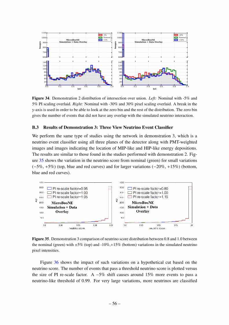
600

700

800

900

1000

1100

Imag

es


-5%

Nominal

+5%

0.0 0.2 0.4 0.6 0.8 1.0IoU

0

20

40

60

80

100

120

140

600

700

800

900

1000

1100

Imag

es


-30%

Nominal

+30%

0.0 0.2 0.4 0.6 0.8 1.0IoU

0

20

40

60

80

100

120

140

Figure 34. Demonstration 2 distribution of intersection over union. Left: Nominal with -5% and5% PI scaling overlaid. Right: Nominal with -30% and 30% pixel scaling overlaid. A break in they-axis is used in order to be able to look at the zero bin and the rest of the distribution. The zero bingives the number of events that did not have any overlap with the simulated neutrino interaction.

B.3 Results of Demonstration 3: Three View Neutrino Event Classifier

We perform the same type of studies using the network in demonstration 3, which is aneutrino event classifier using all three planes of the detector along with PMT-weightedimages and images indicating the location of MIP-like and HIP-like energy depositions.The results are similar to those found in the studies performed with demonstration 2. Fig-ure 35 shows the variation in the neutrino score from nominal (green) for small variations(−5%, +5%) (top, blue and red curves) and for larger variations (−20%, +15%) (bottom,blue and red curves).

Figure 35. Demonstration 3 comparison of neutrino score distribution between 0.8 and 1.0 betweenthe nominal (green) with ±5% (top) and -10%,+15% (bottom) variations in the simulated neutrinopixel intensities.

Figure 36 shows the impact of such variations on a hypothetical cut based on theneutrino score. The number of events that pass a threshold neutrino score is plotted versusthe size of PI re-scale factor. A −5% shift causes around 15% more events to pass aneutrino-like threshold of 0.99. For very large variations, more neutrinos are classified

– 56 –

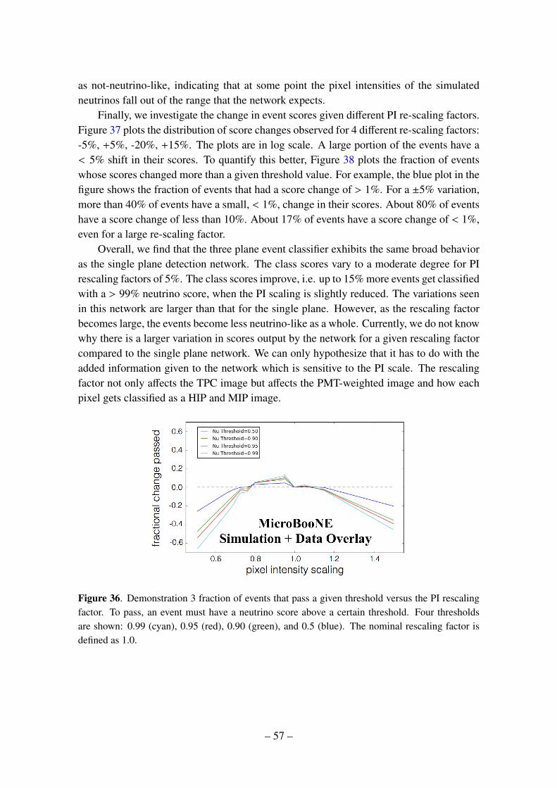
as not-neutrino-like, indicating that at some point the pixel intensities of the simulatedneutrinos fall out of the range that the network expects.

Finally, we investigate the change in event scores given different PI re-scaling factors.Figure 37 plots the distribution of score changes observed for 4 different re-scaling factors:-5%, +5%, -20%, +15%. The plots are in log scale. A large portion of the events have a< 5% shift in their scores. To quantify this better, Figure 38 plots the fraction of eventswhose scores changed more than a given threshold value. For example, the blue plot in thefigure shows the fraction of events that had a score change of > 1%. For a ±5% variation,more than 40% of events have a small, < 1%, change in their scores. About 80% of eventshave a score change of less than 10%. About 17% of events have a score change of < 1%,even for a large re-scaling factor.

Overall, we find that the three plane event classifier exhibits the same broad behavioras the single plane detection network. The class scores vary to a moderate degree for PIrescaling factors of 5%. The class scores improve, i.e. up to 15% more events get classifiedwith a > 99% neutrino score, when the PI scaling is slightly reduced. The variations seenin this network are larger than that for the single plane. However, as the rescaling factorbecomes large, the events become less neutrino-like as a whole. Currently, we do not knowwhy there is a larger variation in scores output by the network for a given rescaling factorcompared to the single plane network. We can only hypothesize that it has to do with theadded information given to the network which is sensitive to the PI scale. The rescalingfactor not only affects the TPC image but affects the PMT-weighted image and how eachpixel gets classified as a HIP and MIP image.

Figure 36. Demonstration 3 fraction of events that pass a given threshold versus the PI rescalingfactor. To pass, an event must have a neutrino score above a certain threshold. Four thresholdsare shown: 0.99 (cyan), 0.95 (red), 0.90 (green), and 0.5 (blue). The nominal rescaling factor isdefined as 1.0.

– 57 –

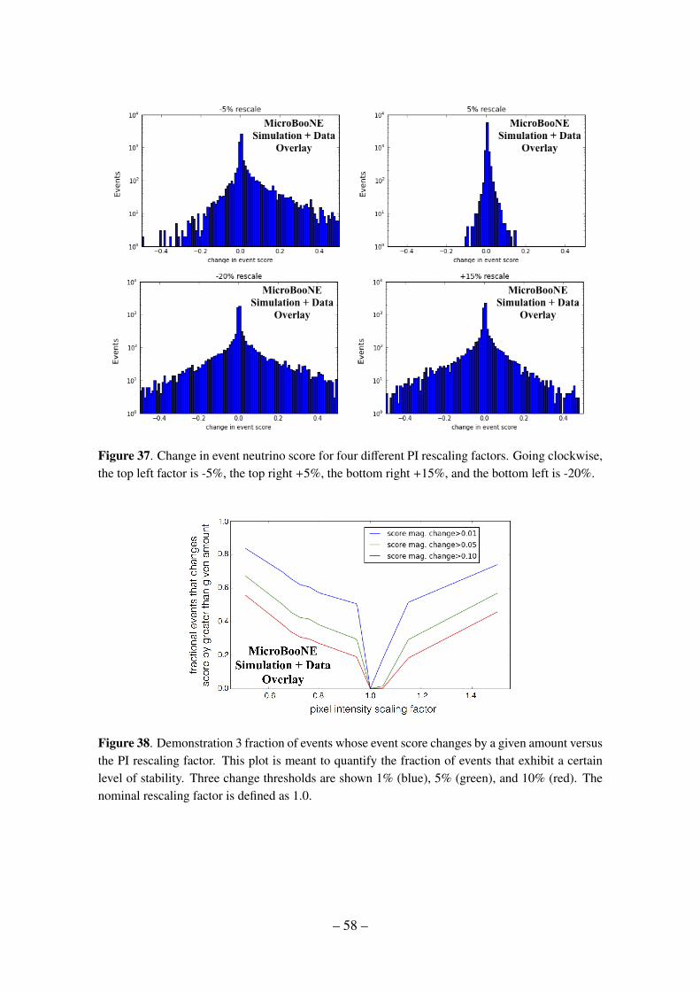
Figure 37. Change in event neutrino score for four different PI rescaling factors. Going clockwise,the top left factor is -5%, the top right +5%, the bottom right +15%, and the bottom left is -20%.

Figure 38. Demonstration 3 fraction of events whose event score changes by a given amount versusthe PI rescaling factor. This plot is meant to quantify the fraction of events that exhibit a certainlevel of stability. Three change thresholds are shown 1% (blue), 5% (green), and 10% (red). Thenominal rescaling factor is defined as 1.0.

– 58 –

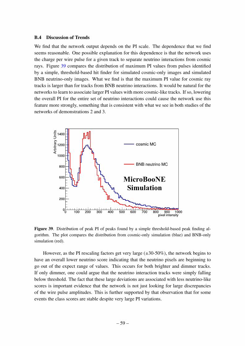
B.4 Discussion of Trends

We find that the network output depends on the PI scale. The dependence that we findseems reasonable. One possible explanation for this dependence is that the network usesthe charge per wire pulse for a given track to separate neutrino interactions from cosmicrays. Figure 39 compares the distribution of maximum PI values from pulses identifiedby a simple, threshold-based hit finder for simulated cosmic-only images and simulatedBNB neutrino-only images. What we find is that the maximum PI value for cosmic raytracks is larger than for tracks from BNB neutrino interactions. It would be natural for thenetworks to learn to associate larger PI values with more cosmic-like tracks. If so, loweringthe overall PI for the entire set of neutrino interactions could cause the network use thisfeature more strongly, something that is consistent with what we see in both studies of thenetworks of demonstrations 2 and 3.

Figure 39. Distribution of peak PI of peaks found by a simple threshold-based peak finding al-gorithm. The plot compares the distribution from cosmic-only simulation (blue) and BNB-onlysimulation (red).

However, as the PI rescaling factors get very large (±30-50%), the network begins tohave an overall lower neutrino score indicating that the neutrino pixels are beginning togo out of the expect range of values. This occurs for both brighter and dimmer tracks.If only dimmer, one could argue that the neutrino interaction tracks were simply fallingbelow threshold. The fact that these large deviations are associated with less neutrino-likescores is important evidence that the network is not just looking for large discrepanciesof the wire pulse amplitudes. This is further supported by that observation that for someevents the class scores are stable despite very large PI variations.

– 59 –

B.5 Discussion of results

The stability against changes in PI indicate that the networks are not just looking for alarge deviation in the PI to find simulated neutrino interactions. If they did, then we wouldexpect the neutrino scores to become larger as the variation increases. This is not observedfor reasonable variations.

Looking to the future, we plan to continue working on properly modeling the PI scalein the simulation. We also plan to investigate how we might mitigate the networks’ sensi-tivity to the PI scale, possibly by using things such as hits to make the image or to explicitlytrain the network to be more stable to modeling errors [28]. Nevertheless, these studiesprovide evidence that the PI scale is used by the network in a non-pathological way, i.e. thenetwork is not just responding to very small or very large differences in the PI for trackscoming from neutrino interactions compared to those from cosmics. However, we do pointout that the PI scale is quite a crude handle. In the future, we plan on looking at varia-tions that distort the pulse shapes. This might include variations in the noise filter on thesimulated wire signals, modeling of space charge effects, or electron lifetime variations.

– 60 –

References

[1] Alex Krizhevsky et al. , “Imagenet Classification with Deep Convolutional NeuralNetworks,” NIPS 25, pages 1106–1114, 2012.

[2] R. Acciarri et al. [SBN Collaboration], “A Proposal for a Three Detector Short-BaselineNeutrino Oscillation Program in the Fermilab Booster Neutrino Beam,” arXiv:1503.01520[physics.ins-det].

[3] R. Acciarri et al. [DUNE Collaboration], “Long-Baseline Neutrino Facility (LBNF) andDeep Underground Neutrino Experiment (DUNE) : Volume 1: The LBNF and DUNEProjects,” arXiv:1601.05471 [physics.ins-det].

[4] E. Racah et al. “Revealing Fundamental Physics from the Daya Bay Neutrino Experimentusing Deep Neural Networks,” arXiv:1601.07621.

[5] A. Aurisano et al., “A Convolutional Neural Network Neutrino Event Classifier,” 2016 JINST11 P09001.

[6] J. Renner et al. [NEXT Collaboration], “Background rejection in NEXT using deep neuralnetworks,” arxiv:1609.06202.

[7] LArSoft release redmine 05.08.00 https://cdcvs.fnal.gov/redmine/projects/larsoft/wiki/ReleaseNotes050800.

[8] uboonecode release redmine 05.08.00 https://cdcvs.fnal.gov/redmine/projects/uboonecode/wiki/ReleaseNotes050800.

[9] Genty, Terao and Wongjirad, LArCV: LArTPC Image Processing/Analysis Framework forDeep Learning https://www.github.com/LArbys/LArCV

[10] Y. Jia et al., “Caffe: Convolutional Architecture for Fast Feature Embedding,”arXiv:1408.5093, 2014.

[11] Christian Szegedy et al., “Going Deeper with Convolutions,” arXiv:1409.4842, 2014.

[12] Ren, Shaoqing and He, Kaiming and Girshick, Ross and Sun, Jian, “Faster R-CNN: TowardsReal-Time Object Detection with Region Proposal Networks,” NIPS 28 pages 91-99, 2015.

[13] Szegedy et al., “Inception-v4, Inception-ResNet and the Impact of Residual Connections onLearning,” arXiv:1602.07261.

[14] Kaiming He et al., “Deep Residual Learning for Image Recognition,” arXiv:1512.03385.

[15] Rene Brun and Fons Rademakers, “ROOT – An object oriented data analysis framework,”NIM A389 81-86, 2015.

[16] NVIDIA GeForce Titan X GPU Card Specification, http://www.geforce.com/hardware/desktop-gpus/geforce-gtx-titan-x/specifications

[17] S. Agostinelli et al., “GEANT4: A Simulation toolkit,” NIM A506 250-303, 2003.

[18] MicroBooNE Collaboration, “TPC Noise Filtering,” MicroBooNE Public Note 1016-PUB.http://www-microboone.fnal.gov/publications/publicnotes/index.html

– 61 –

https://cdcvs.fnal.gov/redmine/projects/larsoft/wiki/ReleaseNotes050800

https://cdcvs.fnal.gov/redmine/projects/larsoft/wiki/ReleaseNotes050800

https://cdcvs.fnal.gov/redmine/projects/uboonecode/wiki/ReleaseNotes050800

https://cdcvs.fnal.gov/redmine/projects/uboonecode/wiki/ReleaseNotes050800

https://www.github.com/LArbys/LArCV

http://www.geforce.com/hardware/desktop-gpus/geforce-gtx-titan-x/specifications

http://www.geforce.com/hardware/desktop-gpus/geforce-gtx-titan-x/specifications

http://www-microboone.fnal.gov/publications/publicnotes/index.html

[19] MicroBooNE Collaboration. “TPC Signal Processing,” MicroBooNE Public Note1017-PUB.http://www-microboone.fnal.gov/publications/publicnotes/index.html

[20] Montavon et al., “Neural Networks: Tricks of the Trade,” Springer 2012.

[21] A. A. Aguilar-Arevalo et al., “The Neutrino Flux Prediction at MiniBooNE,” PRD 78,072002, 2009

[22] C. Andreopoulos et al., “The GENIE Neutrino Monte Carlo Generator,” it NIM A61487-104, 2010.

[23] Ioffe et al., “Batch Normalization: Accelerating Deep Network Training by ReducingInternal Covariate Shift,” Proc. of the 32nd Intl. Conf. on Machine Learning 37, 2015.

[24] Srivastava et al., “Dropout: A Simple Way to Prevent Neural Networks from Overfitting,”Journal of Machine Learning Research 15 1929-1958, 2014.

[25] D. Silver et al., “Mastering the game of Go with deep neural networks and tree search,”Nature 529, 484–489, 2016.

[26] Tieleman, Tijmen and Hinton, Geoffrey. “Lecture 6.5-rmsprop: Divide the gradient by arunning average of its recent magnitude,” COURSERA: Neural Networks for MachineLearning, 4, 2012.

[27] MicroBooNE Collaboration, “Selection and kinematic properties of νµ charged-currentinclusive events in 5e19 POT of MicroBooNE data,” http://www-microboone.fnal.gov/publications/publicnotes/MICROBOONE-NOTE-1010-PUB.pdf

[28] Zheng et al., “Improving the Robustness of Deep Neural Networks via Stability Training,”arXiv:1604.04326.

– 62 –

http://www-microboone.fnal.gov/publications/publicnotes/index.html

http://www-microboone.fnal.gov/publications/publicnotes/MICROBOONE-NOTE-1010-PUB.pdf

http://www-microboone.fnal.gov/publications/publicnotes/MICROBOONE-NOTE-1010-PUB.pdf

convolutional neural networks applied to neutrino · pdf fileconvolutional neural networks...

Documents