convolutional sequence modeling revisited

Under review as a conference paper at ICLR 2018

CONVOLUTIONAL SEQUENCE MODELING REVISITED

Anonymous authorsPaper under double-blind review

ABSTRACT

This paper revisits the problem of sequence modeling using convolutional archi-tectures. Although both convolutional and recurrent architectures have a longhistory in sequence prediction, the current “default” mindset in much of the deeplearning community is that generic sequence modeling is best handled using re-current networks. The goal of this paper is to question this assumption. Specifi-cally, we consider a simple generic temporal convolution network (TCN), whichadopts features from modern ConvNet architectures such as a dilations and resid-ual connections. We show that on a variety of sequence modeling tasks, includ-ing many frequently used as benchmarks for evaluating recurrent networks, theTCN outperforms baseline RNN methods (LSTMs, GRUs, and vanilla RNNs)and sometimes even highly specialized approaches. We further show that the po-tential “infinite memory” advantage that RNNs have over TCNs is largely absentin practice: TCNs indeed exhibit longer effective history sizes than their recurrentcounterparts. As a whole, we argue that it may be time to (re)consider ConvNetsas the default “go to” architecture for sequence modeling.

1 INTRODUCTION

Since the re-emergence of neural networks to the forefront of machine learning, two types of net-work architectures have played a pivotal role: the convolutional network, often used for vision andhigher-dimensional input data; and the recurrent network, typically used for modeling sequentialdata. These two types of architectures have become so ingrained in modern deep learning that theycan be viewed as constituting the “pillars” of deep learning approaches. This paper looks at theproblem of sequence modeling, predicting how a sequence will evolve over time. This is a keyproblem in domains spanning audio, language modeling, music processing, time series forecasting,and many others. Although exceptions certainly exist in some domains, the current “default” think-ing in the deep learning community is that these sequential tasks are best handled by some type ofrecurrent network. Our aim is to revisit this default thinking, and specifically ask whether modernconvolutional architectures are in fact just as powerful for sequence modeling.

Before making the main claims of our paper, some history of convolutional and recurrent modelsfor sequence modeling is useful. In the early history of neural networks, convolutional models werespecifically proposed as a means of handling sequence data, the idea being that one could slide a1-D convolutional filter over the data (and stack such layers together) to predict future elements of asequence from past ones (Hinton, 1989; LeCun et al., 1995). Thus, the idea of using convolutionalmodels for sequence modeling goes back to the beginning of convolutional architectures themselves.However, these models were subsequently largely abandoned for many sequence modeling tasks infavor of recurrent networks (Elman, 1990). The reasoning for this appears straightforward: whileconvolutional architectures have a limited ability to look back in time (i.e., their receptive field islimited by the size and layers of the filters), recurrent networks have no such limitation. Because re-current networks propagate forward a hidden state, they are theoretically capable of infinite memory,the ability to make predictions based upon data that occurred arbitrarily long ago in the sequence.This possibility seems to be realized even moreso for the now-standard architectures of Long Short-Term Memory networks (LSTMs) (Hochreiter & Schmidhuber, 1997), or recent incarnations suchas the Gated Recurrent Unit (GRU) (Cho et al., 2014); these architectures aim to avoid the “vanish-ing gradient” challenge of traditional RNNs and appear to provide a means to actually realize thisinfinite memory.

1


Given the substantial limitations of convolutional architectures at the time that RNNs/LSTMs wereinitially proposed (when deep convolutional architectures were difficult to train, and strategies suchas dilated convolutions had not reached widespread use), it is no surprise that CNNs fell out offavor to RNNs. While there have been a few notable examples in recent years of CNNs appliedto sequence modeling (e.g., the WaveNet (Oord et al., 2016a) and PixelCNN (Oord et al., 2016b)architectures), the general “folk wisdom” of sequence modeling prevails, that the first avenue ofattack for these problems should be some form of recurrent network.

The fundamental aim of this paper is to revisit this folk wisdom, and thereby make a counterclaim.We argue that with the tools of modern convolutional architectures at our disposal (namely the abilityto train very deep networks via residual connections and other similar mechanisms, plus the abilityto increase receptive field size via dilations), in fact convolutional architectures typically outperformrecurrent architectures on sequence modeling tasks, especially (and perhaps somewhat surprisingly)on domains where a long effective history length is needed to make proper predictions.

This paper consists of two main contributions. First, we describe a generic, baseline temporal convo-lutional network (TCN) architecture, combining best practices in the design of modern convolutionalarchitectures, including residual layers and dilation. We emphasize that we are not claiming to in-vent the practice of applying convolutional architectures to sequence prediction, and indeed the TCNarchitecture here mirrors closely architectures such as WaveNet (in fact TCN is notably simpler insome respects). We do, however, want to propose a generic modern form of convolutional sequenceprediction for subsequent experimentation. Second, and more importantly, we extensively evaluatethe TCN model versus alternative approaches on a wide variety of sequence modeling tasks, span-ning many domains and datasets that have typically been the purview of recurrent models, includingword- and character-level language modeling, polyphonic music prediction, and other baseline taskscommonly used to evaluate recurrent architectures. Although our baseline TCN can be outperformedby specialized (and typically highly-tuned) RNNs in some cases, for the majority of problems theTCN performs best, with minimal tuning on the architecture or the optimization. This paper alsoanalyzes empirically the myth of “infinite memory” in RNNs, and shows that in practice, TCNsof similar size and complexity may actually demonstrate longer effective history sizes. Our chiefclaim in this paper is thus an empirical one: rather than presuming that RNNs will be the defaultbest method for sequence modeling tasks, it may be time to (re)consider ConvNets as the “go-to”approach when facing a new dataset or task in sequence modeling.

2 RELATED WORK

In this section we highlight some of the key innovations in the history of recurrent and convolutionalarchitectures for sequence prediction.

Recurrent networks broadly refer to networks that maintain a vector of hidden activations, which arekept over time by propagating them through the network. The intuitive appeal of this approach is thatthe hidden state can act as a sort of “memory” of everything that has been seen so far in a sequence,without the need for keeping an explicit history. Unfortunately, such memory comes at a cost, andit is well-known that the naıve RNN architecture is difficult to train due to the exploding/vanishinggradient problem (Bengio et al., 1994).

A number of solutions have been proposed to address this issue. More than twenty yearsago, Hochreiter & Schmidhuber (1997) introduced the now-ubiquitous Long Short-Term Memory(LSTM) which uses a set of gates to explicitly maintain memory cells that are propagated forwardin time. Other solutions or refinements include a simplified variant of LSTM, the Gated RecurrentUnit (GRU) (Cho et al., 2014), peephole connections (Gers et al., 2002), Clockwork RNN (Koutniket al., 2014) and recent works such as MI-RNN (Wu et al., 2016) and the Dilated RNN (Chang et al.,2017). Alternatively, several regularization techniques have been proposed to better train LSTMs,such as those based upon the properties of the RNN dynamical system (Pascanu et al., 2013); morerecently, strategies such as Zoneout (Krueger et al., 2017) and AWD-LSTM (Merity et al., 2017)were also introduced to regularize LSTM in various ways, and have achieved exceptional results inthe field of language modeling.

While it is frequently criticized as a seemingly “ad-hoc” architecture, LSTMs have proven to beextremely robust and is very hard to improve upon by other recurrent architectures, at least for

2


general problems. Jozefowicz et al. (2015) concluded that if there were “architectures much betterthan the LSTM”, then they were “not trivial to find”. However, while they evaluated a variety ofrecurrent architectures with different combinations of components via an evolutionary search, theydid not consider architectures that were fundamentally different from the recurrent ones.

The history of convolutional architectures for time series is comparatively shorter, as they soon fellout of favor compared to recurrent architectures for these tasks, though are also seeing a resurgencein recent years. Waibel et al. (1989) and Bottou et al. (1990) studied the usage of time-delay net-works (TDNNs) for sequences, one of the earliest local-connection-based networks in this domain.LeCun et al. (1995) then proposed and examined the usage of CNNs on time-series data, pointingout that the same kind of feature extraction used in images could work well on sequence model-ing with convolutional filters. Recent years have seen a re-emergence of convolutional models forsequence data. Perhaps most notably, the WaveNet (Oord et al., 2016a) applied a stacked convolu-tional architecture to model audio signals, using a combination of dilations (Yu & Koltun, 2015),skip connections, gating, and conditioning on context stacks; the WaveNet mode was additionallyapplied to a few other contexts, such as financial applications (Borovykh et al., 2017). Non-dilatedgated convolutions have also been applied in the context of language modeling (Dauphin et al.,2017). And finally, convolutional models have seen a recent adoption in sequence to sequence mod-eling and machine translations applications, such as the ByteNet (Kalchbrenner et al., 2016) andConvS2S architectures (Gehring et al., 2017).

Despite these successes, the general consensus of the deep learning community seems to be thatRNNs (here meaning all RNNs including LSTM and its variants) are better suited to sequence mod-eling for two apparent reasons: 1) as discussed before, RNNs are theoretically capable of infinitememory; and 2) RNN models are inherently suitable for sequential inputs of varying length, whereasCNNs seem to be more appropriate in domains with fixed-size inputs (e.g., vision).

With this as the context, this paper reconsiders convolutional sequence modeling in general, firstintroducing a simple general-purpose convolutional sequence modeling architecture that can be ap-plied in all the same scenarios as an RNN (the architecture acts as a “drop-in” replacement for RNNsof any kind). We then extensively evaluate the performance of the architecture on tasks from dif-ferent domains, focusing on domains and settings that have been used explicitly as applications andbenchmarks for RNNs in the recent past. With regard to the specific architectures mentioned above(e.g. WaveNet, ByteNet, gated convolutional language models), the primary goal here is to describea simple, application-independent architecture that avoids much of the extra specialized componentsof these architectures (gating, complex residuals, context stacks, or the encoder-decoder architec-tures of seq2seq models), and keeps only the “standard” convolutional components from most imagearchitectures, with the restriction that the convolutions be causal. In several cases we specificallycompare the architecture with and without additional components (e.g., gating elements), and high-light that it does not seem to substantially improve performance of the architecture across domains.Thus, the primary goal of this paper is to provide a baseline architecture for convolutional sequenceprediction tasks, and to evaluate the performance of this model across multiple domains.

3 CONVOLUTIONAL SEQUENCE MODELING

In this section, we propose a generic architecture for convolutional sequence prediction, and gen-erally refer to it as Temporal Convolution Networks (TCNs). We emphasize that we adopt thisterm not as a label for a truly new architecture, but as a simple descriptive term for this and similararchitectures. The distinguishing characteristics of the TCN are that: 1) the convolutions in the ar-chitecture are causal, meaning that there is no information “leakage” between future and past; 2) thearchitecture can take a sequence of any length and map it to an output sequence of the same length,just as with an RNN. Beyond this, we emphasize how to build very long effective history sizes (i.e.,the ability for the networks to look very far into the past to make a prediction) using a combinationof very deep networks (augmented with residual layers) and dilated convolutions.

3.1 THE SEQUENCE MODELING TASK

Before defining the network structure, we highlight the nature of the sequence modeling task. Wesuppose that we are given a sequence of inputs x0, . . . , xT , and we wish to predict some correspond-

3


x0 x1 xT. . .

yTyT�1

xT�1

f(x

0,.

..,x

T)

Future direction

Input

Hidden

Output. . .

. . .

Figure 1: A simple causal convolution with filter size 3.

ing outputs y0, . . . , yT at each time. The key constraint is that to predict the output yt for some timet, we are constrained to only use those inputs that have been previously observed: x0, . . . , xt. For-mally, a sequence modeling network is any function f : X T+1 → YT+1 that produces this mapping

y0, . . . , yT = f(x0, . . . , xT ) (1)

if it satisfies the causal constraint that yt depends only on x0, . . . , xt, and not on any “future” inputsxt+1, . . . , xT . The goal of learning in the sequence modeling setting is to find the network f mini-mizing some expected loss between the actual outputs and predictionsL(y0, . . . , yT , f(x0, . . . , xT ))where the sequences and outputs are drawn according to some distribution.

This formalism encompasses many settings such as auto-regressive prediction (where we try topredict some signal given its past) by setting the target output to be simply the input shifted by onetime step. It does not, however, directly capture domains such as machine translation, or sequence-to-sequence prediction in general, since in these cases the entire input sequence (including “future”states) can be used to predict each output (though the techniques can naturally be extended to workin such settings).

3.2 CAUSAL CONVOLUTIONS AND THE TCN

As mentioned above, the TCN is based upon two principles: the fact that the network produces anoutput of the same length as the input, and the fact that there can be no leakage from the futureinto the past. To accomplish the first point, the TCN uses a 1D fully-convolutional network (FCN)architecture (Long et al., 2015), where each hidden layer is the same length as the input layer, andzero padding of length (kernel size − 1) is added to keep subsequent layers the same length asprevious ones. To achieve the second point, the TCN uses causal convolutions, convolutions wherea subsequent output at time t is convolved only with elements from time t and before in the previouslayer.1 Graphically, the network is shown in Figure 1. Put in a simple manner:

TCN = 1D FCN + causal convolutions

It is worth emphasizing that this is essentially the same architecture as the time delay neural networkproposed nearly 30 years ago by Waibel et al. (1989), with the sole tweak of zero padding to ensureequal sizes of all layers.

However, a major disadvantage of this “naıve” approach is that in order to achieve a long effectivehistory size, we need an extremely deep network or very large filters, neither of which were particu-larly feasible when the methods were first introduced. Thus, in the following sections, we describehow techniques from modern convolutional architectures can be integrated into the TCN to allowfor both very deep networks and very long effective history.

1Although many current deep learning libraries do not offer native support for these causal convolutions,we note that they can be implemented (with some inefficiency) by simply using a standard convolution withzero padding on both sides, and chopping off the end of the sequence.

4


. . .

x0 x1 xT�1 xT. . .

y1y0 yTyT�1. . .

Input

Hidden

Hidden

Output

d = 1

d = 2

d = 4

Padding = 2

Padding = 4

Padding = 8

x2 xT�2

yT�2y2

Figure 2: A dilated causal convolution with dilation factors d = 1, 2, 4 and filter size k = 3. Thereceptive field is able to cover all values from the input sequence.

3.3 DILATED CONVOLUTIONS

Through convolutional filters, as previously addressed, a simple causal convolution is only able tolook back at a history with size linear in the depth of the network. This makes it challenging toapply the aforementioned causal convolution on sequence tasks, especially those requiring longerhistory. Our solution here, used previously for example in audio synthesis by Oord et al. (2016a),is to employ dilated convolutions (Yu & Koltun, 2015) that enable an exponentially large receptivefield. More formally, for a 1-D sequence input x ∈ Rn and a filter f : {0, . . . , k − 1} → R, thedilated convolution operation F on element s of the sequence is defined as

F (s) = (x ∗d f)(s) =k−1∑i=0

f(i) · xs+d·i

where d is the dilation factor and k is the filter size. Dilation is thus equivalent to introducing a fixedstep between every two adjacent filter taps. When taking d = 1, for example, a dilated convolutionis trivially a normal convolution operation. Using larger dilations enables an output at the top levelto represent a wider range of inputs, thus effectively expanding the receptive field of a ConvNet.

This gives us two ways to increase the receptive field of the TCN: by choosing larger filter sizes k,and by increasing the dilation factor d, where the effective history of one such layer is (k − 1)d.As is common when using dilated convolutions, we increase d exponentially with the depth of thenetwork (i.e., d = O(2i) at level i of the network). This ensures that there is some filter that hitseach input within the effective history, while also allowing for an extremely large effective historyusing deep networks. We provide an illustration in Figure 2. Using filter size k = 3 and dilationfactor d = 1, 2, 4, the receptive field is able to cover all values from the input sequence.

3.4 RESIDUAL CONNECTIONS

Proposed by He et al. (2016), residual functions have proven to be especially useful in effectivelytraining deep networks. In a residual network, each residual block contains a branch leading out toa series of transformations F , whose outputs are added to the input x of the block:

o = Activation(x+ F(x))This effectively allows for the layers to learn modifications to the identity mapping rather than theentire transformation, which has been repeatedly shown to benefit very deep networks.

As the TCN’s receptive field depends on the network depth n as well as filter size k and dilationfactor d, stabilization of deeper and larger TCNs becomes important. For example, in a case wherethe prediction could depend on a history of size 212 and a high-dimensional input sequence, a net-work of up to 12 layers could be needed. Each layer, more specifically, consists of multiple filtersfor feature extraction. In our design of the generic TCN model, we therefore employed a genericresidual module in place of a convolutional layer.

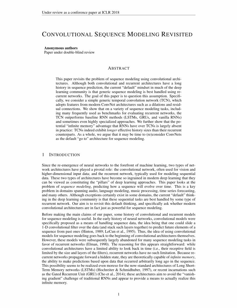
The residual block for our baseline TCN is shown in figure 3a. Within a residual block, the TCN has2 layers of dilated causal convolution and non-linearity, for which we used the rectified linear unit

5


Residual block (k, d)

1x1 Conv (optional)

WeightNorm

Dilated Causal Conv

ReLU

Dropout

WeightNorm

Dilated Causal Conv

ReLU

Dropout +

z(i) = (z(i)1 , . . . , z

(i)T )

z(i�1) = (z(i�1)1 , . . . , z

(i�1)T )

(a) TCN residual block. An 1x1 convolution isadded when residual input and output have dif-ferent dimensions.

x0 x1 xT. . . xT�1

. . .

+++

z(1)T�1 z

(1)T

Residual block (k=2, d=1)

Convolutional FilterIdentity Map (or 1x1 Conv)

(b) An example of residual connection in TCN.The blue lines are filters in the residual function,and the green lines are identity mappings.

Figure 3: A visualization of the TCN residual block

(ReLU) (Nair & Hinton, 2010). For normalization, we applied Weight Normalization (Salimans &Kingma, 2016) to the filters in the dilated convolution (where we note that the filters are essentiallyvectors of size k × 1). In addition, a 2-D dropout (Srivastava et al., 2014) layer was added aftereach dilated convolution for regularization: at each training step, a whole channel (in the widthdimension) is zeroed out.

However, whereas in standard ResNet the input is passed in and added directly to the output of theresidual function, in TCN (and ConvNet in general) the input and output could have different widths.Therefore in our TCN, when the input-output widths disagree, we use an additional 1x1 convolutionto ensure that element-wise addition ⊕ receives tensors of the same shape (see Figure 3a, 3b).

Note that many further optimizations (e.g., gating, skip connections, context stacking as in audiogeneration using WaveNet) are possible in a TCN than what we described here. However, in thispaper, we aim to present a generic, general-purpose TCN, to which additional twists can be addedas needed. As we are going to show in Section 4, this general-purpose architecture is already ableto outperform recurrent units like LSTM on a number of tasks by a good margin.

3.5 ADVANTAGES OF TCN SEQUENCE MODELING

There are several key advantages to a TCN model with the ingredients that we described above.

• Parallelism. Unlike in RNNs where the predictions for later timesteps must wait for theirpredecessors to complete, in a convolutional architecture these computations can be donein parallel since the same filter is used in each layer. Therefore, in training and evaluation,a (possibly long) input sequence can be processed as a whole in TCN, instead of serially asin RNN, which depends on the length of the sequence and could be less efficient.

• Flexible receptive field size. With a TCN, we can change its receptive field size in mul-tiple ways. For instance, stacking more dilated (causal) convolutional layers, using largerdilation factors, or increasing the filter size are all viable options (with possibly differentinterpretations). TCN is thus easy to tune and adapt to different domains, since we now candirectly control the size of the model’s memory.

• Stable gradients. Unlike recurrent architectures, TCN has a backpropagation path that isdifferent from the temporal direction of the sequence. This enables it to avoid the problemof exploding/vanishing gradients, which is a major issue for RNNs (and which led to thedevelopment of LSTM, GRU, HF-RNN, etc.).

• Low memory requirement for training. In a task where the input sequence is long,a structure such as LSTM can easily use up a lot of memory to store the partial resultsfor backpropagation (e.g., the results for each gate of the cell). However, in TCN, the

6


backpropagation path only depends on the network depth and the filters are shared in eachlayer, which means that in practice, as model size or sequence length gets large, TCN islikely to use less memory than RNNs.

3.6 DISADVANTAGES OF TCN SEQUENCE MODELING

We also summarize two disadvantages of using TCN instead of RNNs.

• Data storage in evaluation. In evaluation/testing, RNNs only need to maintain a hiddenstate and take in a current input xt in order to generate a prediction. In other words, a“summary” of the entire history is provided by the fixed-length set of vectors ht, whichmeans that the actual observed sequence can be discarded (and indeed, the hidden state canbe used as a kind of encoder for all the observed history). In contrast, the TCN still needsto take in a sequence with non-trivial length (precisely the effective history length) in orderto predict, thus possibly requiring more memory during evaluation.

• Potential parameter change for a transfer of domain. Different domains can have dif-ferent requirements on the amount of history the model needs to memorize. Therefore,when transferring a model from a domain where only little memory is needed (i.e., small kand d) to a domain where much larger memory is required (i.e., much larger k and d), TCNmay perform poorly for not having a sufficiently large receptive field.

We want to emphasize, though, that we believe the notable lack of “infinite memory” for a TCN isdecidedly not a practical disadvantage, since, as we show in Section 4, the TCN method actuallyoutperforms RNNs in terms of the ability to deal with long temporal dependencies.

4 EXPERIMENTS

In this section, we conduct a series of experiments using the baseline TCN (described in section 3)and generic RNNs (namely LSTMs, GRUs, and vanilla RNNs). These experiments cover tasks anddatasets from various domains, aiming to test different aspects of a model’s ability to learn sequencemodeling. In several cases, specialized RNN models, or methods with particular forms of regulariza-tion can indeed vastly outperform both generic RNNs and the TCN on particular problems, whichwe highlight when applicable. But as a general-purpose architecture, we believe the experimentsmake a compelling case for the TCN as the “first attempt” approach for many sequential problems.

All experiments reported in this section used the same TCN architecture, just varying the depth of thenetwork and occasionally the kernel size. We use an exponential dilation d = 2n for layer n in thenetwork, and the Adam optimizer (Kingma & Ba, 2015) with learning rate 0.002 for TCN (unlessotherwise noted). We also empirically find that gradient clipping helped training convergence ofTCN, and we pick the maximum norm to clip from [0.3, 1]. When training recurrent models, weuse a simple grid search to find a good set of hyperparameters (in particular, optimizer, recurrentdrop p ∈ [0.05, 0.5], the learning rate, gradient clipping, and initial forget-gate bias), while keepingthe network around the same size as TCN. No other optimizations, such as gating mechanism (seeAppendix D), or highway network, were added to TCN or the RNNs. The hyperparameters we usefor TCN on different tasks are reported in Table 2 in Appendix B. In addition, we conduct a seriescontrolled experiments to investigate the effects of filter size and residual function on the TCN’sperformance. These results can be found in Appendix C.

4.1 TASKS AND RESULTS SUMMARY

In this section we highlight the general performance of generic TCNs vs generic LSTMs for a varietyof domains from the sequential modeling literature. A complete description of each task, as wellas references to some prior works that evaluated them, is given in Appendix A. In brief, the taskswe consider are: the adding problem, sequential MNIST, permuted MNIST (P-MNIST), the copymemory task, the Nottingham and JSB Chorales polyphonic music tasks, Penn Treebank (PTB),Wikitext-103 and LAMBADA word-level language modeling, as well as PTB and text8 character-level language modeling.

7


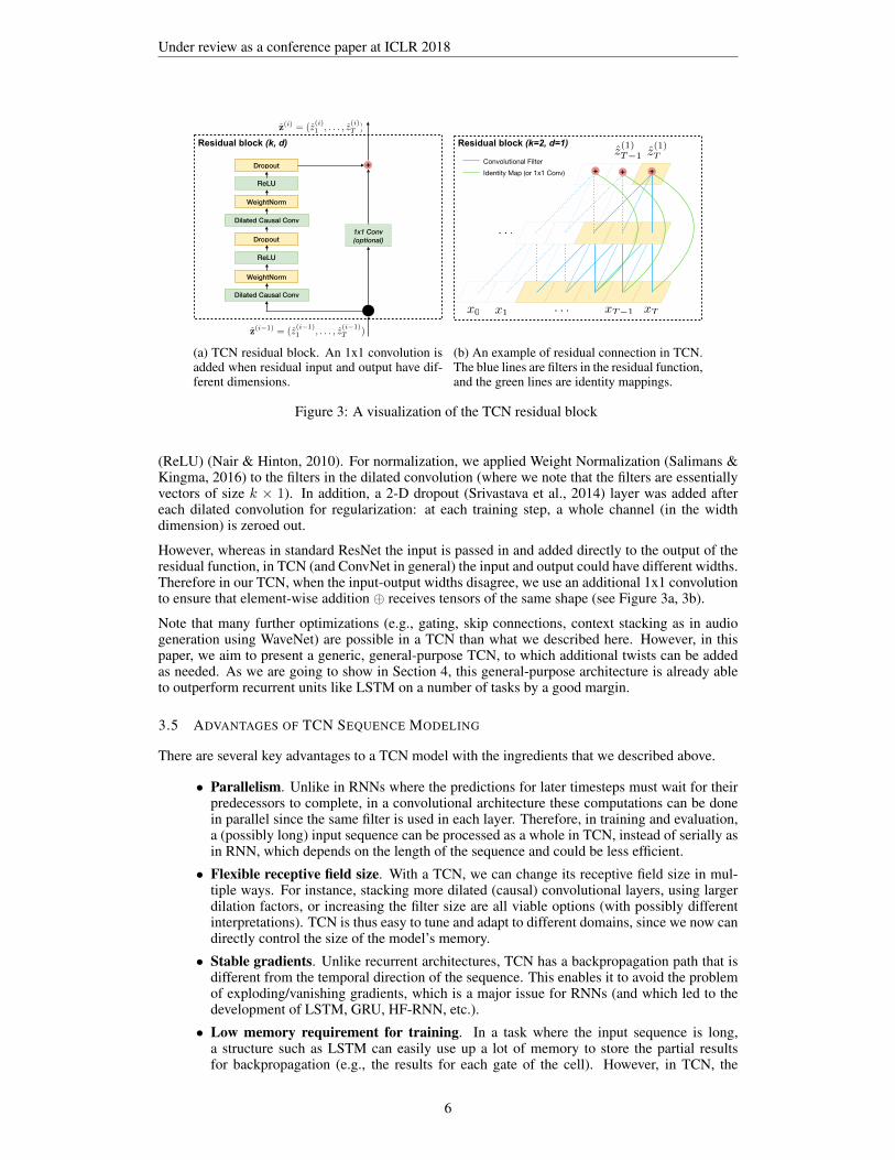
Table 1: Complete comparison of the TCN to regularized recurrent architectures in various tasks.

Sequential Tasks Model Size (≈)Models

LSTM GRU RNN TCN (ours)

Seq. MNIST (accuracy) 70K 87.2 96.2 21.5 99.0P-Seq. MNIST (accuracy) 70K 85.7 87.3 25.3 97.2The Adding Problem T=600 (loss) 70K 0.164 5.3e-5 0.177 5.8e-5Copy Memory T=1000 (loss) 16K 0.0204 0.0197 - 3.5e-5Music JSB Chorales (loss) 300K 8.45 8.43 8.91 8.10Music Nottingham (loss) 1M 3.29 3.46 - 3.07Word-level PTB (ppl) 13M 84.77 92.48 114.50 90.17Word-level Wiki-103 (ppl) - 48.4 (large) - - 45.19Word-level LAMBADA (ppl) - 4186 - 14725 1279Char-level PTB (bpc) 3M 1.41 1.42 1.52 1.35Char-level text8 (bpc) 5M 1.52 1.56 1.69 1.45

(a) T = 200 (b) T = 400 (c) T = 600

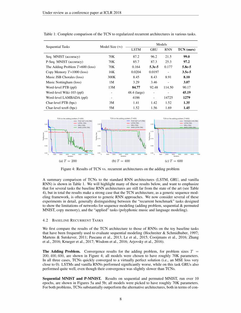
Figure 4: Results of TCN vs. recurrent architectures on the adding problem

A summary comparison of TCNs to the standard RNN architectures (LSTM, GRU, and vanillaRNN) is shown in Table 1. We will highlight many of these results below, and want to emphasizethat for several tasks the baseline RNN architectures are still far from the state of the art (see Table4), but in total the results make a strong case that the TCN architecture, as a generic sequence mod-eling framework, is often superior to generic RNN approaches. We now consider several of theseexperiments in detail, generally distinguishing between the “recurrent benchmark” tasks designedto show the limitations of networks for sequence modeling (adding problem, sequential & permutedMNIST, copy memory), and the “applied” tasks (polyphonic music and language modeling).

4.2 BASELINE RECURRENT TASKS

We first compare the results of the TCN architecture to those of RNNs on the toy baseline tasksthat have been frequently used to evaluate sequential modeling (Hochreiter & Schmidhuber, 1997;Martens & Sutskever, 2011; Pascanu et al., 2013; Le et al., 2015; Cooijmans et al., 2016; Zhanget al., 2016; Krueger et al., 2017; Wisdom et al., 2016; Arjovsky et al., 2016).

The Adding Problem. Convergence results for the adding problem, for problem sizes T =200, 400, 600, are shown in Figure 4; all models were chosen to have roughly 70K parameters.In all three cases, TCNs quickly converged to a virtually perfect solution (i.e., an MSE loss veryclose to 0). LSTMs and vanilla RNNs performed significantly worse, while on this task GRUs alsoperformed quite well, even though their convergence was slightly slower than TCNs.

Sequential MNIST and P-MNIST. Results on sequential and permuted MNIST, run over 10epochs, are shown in Figures 5a and 5b; all models were picked to have roughly 70K parameters.For both problems, TCNs substantially outperform the alternative architectures, both in terms of con-

8


(a) Sequential MNIST (b) P-MNIST

Figure 5: Results of TCN vs. recurrent architectures on the Sequential MNIST and P-MNIST

(a) T = 500. (b) T = 1000. (c) T = 2000.

Figure 6: Result of TCN vs. recurrent architectures on the Copy Memory Task, for different T

vergence time and final performance level on the task. For the permuted sequential MNIST, TCNsoutperform state of the art results using recurrent nets (95.9%) with Zoneout+Recurrent BatchNorm(Cooijmans et al., 2016; Krueger et al., 2017), a highly optimized method for regularizing RNNs.

Copy Memory Task. Finally, Figure 6 shows the results of the different methods (with roughlythe same size) on the copy memory task. Again, the TCNs quickly converge to correct answers,while the LSTM and GRU simply converge to the same loss as predicting all zeros. In this case wealso compare to the recently-proposed EURNN (Jing et al., 2017), which was highlighted to performwell on this task. While both perform well for sequence length T = 500, the TCN again has a clearadvantage for T = 1000 and T = 2000 (in terms of both loss and convergence).

4.3 RESULTS ON POLYPHONIC MUSIC AND LANGUAGE MODELING

Next, we compare the results of the TCN architecture to recurrent architectures on 6 different realdatasets in polyphonic music as well as word- and character-level language modeling. These areareas where sequence modeling has been used most frequently. As domains where there is consider-able practical interests, there have also been many specialized RNNs developed for these tasks (e.g.,Zhang et al. (2016); Ha et al. (2017); Krueger et al. (2017); Grave et al. (2016); Greff et al. (2017);Merity et al. (2017)). We mention some of these comparisons when useful, but the primary goalhere is to compare the generic TCN model to other generic RNN architectures, so we focus mainlyon these comparisons.

Polyphonic Music. On the Nottingham and JSB Chorales datasets, the TCN with virtually notuning is again able to beat the other models by a considerable margin (see Table 1), and even out-performs some improved recurrent models for this task such as HF-RNN (Boulanger-Lewandowskiet al., 2012) and Diagonal RNN (Subakan & Smaragdis, 2017). Note however that other modelssuch as the Deep Belief Net LSTM (Vohra et al., 2015) perform substantially better on this task;we believe this is likely due to the fact that the datasets involved in polyphonic music are relatively

9


small, and thus the right regularization method or generative modeling procedure can improve per-formance significantly. This is largely orthogonal to the RNN/TCN distinction, as a similar variantof TCN may well be possible.

Word-level Language Modeling. Language modeling remains one of the primary applicationsof recurrent networks in general, where many recent works have been focusing on optimizing theusage of LSTMs (see Krueger et al. (2017); Merity et al. (2017)). In our implementation, we followstandard practices such as tying the weights of encoder and decoder layers for both TCN and RNNs(Press & Wolf, 2016), which significantly reduces the number of parameters in the model. Whentraining the language modeling tasks, we use SGD optimizer with annealing learning rate (by afactor of 0.5) for TCN and RNNs.

Results on word-level language modeling are reported in Table 1. With a fine-tuned LSTM (i.e., withrecurrent and embedding dropout, etc.), we find LSTM can outperform TCN in perplexity on thePenn TreeBank (PTB) dataset, where the TCN model still beats both GRU and vanilla RNN. On themuch larger Wikitext-103 corpus, however, without performing much hyperparameter search (dueto lengthy training process), we still observe that TCN outperforms the state of the art LSTM results(48.4 in perplexity) by Grave et al. (2016) (without continuous cache pointer; see Table 4). Thesame superiority is observed on the LAMBADA test (Paperno et al., 2016), where TCN achievesa much lower perplexity than its recurrent counterparts in predicting the last word based on a verylong context (see Appendix A). We will further analyze this in section 4.4.

Character-level Language Modeling. The results of applying TCN and alternative models onPTB and text8 data for character-level language modeling are shown in Table 1, with performancemeasured in bits per character (bpc). While beaten by the state of the art (see Table 4), the genericTCN outperforms regularized LSTM and GRU as well as methods such as Norm-stabilized LSTM(Krueger & Memisevic, 2015). Moreover, we note that using a filter size of k ≤ 4 works better thanlarger filter sizes in character-level language modeling, which suggests that capturing short historyis more important than longer dependencies in these tasks.

4.4 MEMORY SIZE OF TCN AND RNNS

Finally, one of the important reasons why RNNs have been preferred over CNNs for general se-quence modeling is that theoretically, recurrent architectures are capable of an infinite memory.We therefore attempt to study here how much memory TCN and LSTM/GRU are able to actually“backtrack”, via the copy memory task and the LAMBADA language modeling task.

Figure 7: Accuracy on the copy memory taskfor varying sequence length T .

The copy memory task is a simple but perfect taskto examine a model’s ability to pick up its memoryfrom a (possibly) distant past (by varying the valueof sequence length T ). However, different from thesetting in Section 4.2, in order to compare the resultsfor different sequence lengths, here we only reportthe accuracy on the last 10 elements of the outputsequence. We used a model size of 10K for bothTCN and RNNs.

The results are shown in Figure 7. TCNs consis-tently converge to 100% accuracy for all sequencelengths, whereas it is increasingly challenging for re-current models to memorize as T grows (with accu-racy converging to that of a random guess). LSTM’saccuracy quickly falls below 20% for T ≥ 50, whichsuggests that instead of infinite memory, LSTMs areonly good at recalling a short history instead.

This observation is also backed up by the experi-ments of TCN on the LAMBADA dataset, which is

specifically designed to test a model’s textual understanding in a broader discourse. The objectiveof LAMBADA dataset is to predict the last word of the target sentence given a sufficiently long

10


context (see Appendix A for more details). Most of the existing models fail to guess accurately onthis task. As shown in Table 1, TCN outperforms LSTMs by a significant margin in perplexity onLAMBADA (with a smaller network and virtually no tuning).

These results indicate that TCNs, despite their apparent finite history, in practice maintain a longereffective history than their recurrent counterparts. We would like to emphasize that this empiricalobservation does not contradict the good results that prior works have achieved using LSTM, suchas in language modeling on PTB. In fact, the very success of n-gram models (Brown et al., 1992)suggested that language modeling might not need a very long memory, a conclusion also reached byprior works such as Dauphin et al. (2017).

5 DISCUSSION

In this work, we revisited the topic of modeling sequence predictions using convolutional archi-tectures. We introduced the key components of the TCN and analyzed some vital advantages anddisadvantages of using TCN for sequence predictions instead of RNNs. Further, we compared ourgeneric TCN model to the recurrent architectures on a set of experiments that span a wide range ofdomains and datasets. Through these experiments, we have shown that TCN with minimal tuningcan outperform LSTM/GRU of the same model size (and with standard regularizations) in most ofthe tasks. Further experiments on the copy memory task and LAMBADA task revealed that TCNsactually has a better capability for long-term memory than the comparable recurrent architectures,which are commonly believed to have unlimited memory.

It is still important to note that, however, we only presented a generic architecture here, with com-ponents all coming from standard modern convolutional networks (e.g., normalization, dropout,residual network). And indeed, on specific problems, the TCN model can still be beaten by somespecialized RNNs that adopt carefully designed optimization strategies. Nevertheless, we believethe experiment results in Section 4 might be a good signal that instead of considering RNNs as the“default” methodology for sequence modeling, convolutional networks too, can be a promising andpowerful toolkit in studying time-series data.

REFERENCES

Allan, M. and Williams, C. Harmonising chorales by probabilistic inference. In Advances in neuralinformation processing systems, pp. 25–32, 2005.

Arjovsky, M., Shah, A., and Bengio, Y. Unitary evolution recurrent neural networks. In InternationalConference on Machine Learning (ICML-16), pp. 1120–1128, 2016.

Bengio, Y., Simard, P., and Frasconi, P. Learning long-term dependencies with gradient descent isdifficult. IEEE transactions on neural networks, 5(2):157–166, 1994.

Borovykh, A., Bohte, S., and Oosterlee, C. W. Conditional time series forecasting with convolutionalneural networks. arXiv preprint arXiv:1703.04691, 2017.

Bottou, L., Soulie, F. F., Blanchet, P., and Lienard, J.-S. Speaker-independent isolated digit recog-nition: Multilayer perceptrons vs. dynamic time warping. Neural Networks, 3(4):453–465, 1990.

Boulanger-Lewandowski, N., Bengio, Y., and Vincent, P. Modeling temporal dependencies in high-dimensional sequences: Application to polyphonic music generation and transcription. arXivpreprint arXiv:1206.6392, 2012.

Brown, P. F., Desouza, P. V., Mercer, R. L., Pietra, V. J. D., and Lai, J. C. Class-based n-gram modelsof natural language. Computational linguistics, 18(4):467–479, 1992.

Chang, S., Zhang, Y., Han, W., Yu, M., Guo, X., Tan, W., Cui, X., Witbrock, M., Hasegawa-Johnson,M., and Huang, T. Dilated recurrent neural networks. arXiv preprint arXiv:1710.02224, 2017.

Cho, K., Van Merrienboer, B., Bahdanau, D., and Bengio, Y. On the properties of neural machinetranslation: Encoder-decoder approaches. arXiv preprint arXiv:1409.1259, 2014.

11


Chung, J., Gulcehre, C., Cho, K., and Bengio, Y. Empirical evaluation of gated recurrent neuralnetworks on sequence modeling. arXiv preprint arXiv:1412.3555, 2014.

Chung, J., Ahn, S., and Bengio, Y. Hierarchical multiscale recurrent neural networks. arXiv preprintarXiv:1609.01704, 2016.

Cooijmans, T., Ballas, N., Laurent, C., Gulcehre, C., and Courville, A. Recurrent batch normaliza-tion. In International Conference on Learning Representations, 2016.

Dauphin, Y. N., Fan, A., Auli, M., and Grangier, D. Language modeling with gated convolutionalnetworks. In International Conference on Machine Learning (ICML-17), pp. 933–941, 2017.

Elman, J. L. Finding structure in time. Cognitive science, 14(2):179–211, 1990.

Gehring, J., Auli, M., Grangier, D., Yarats, D., and Dauphin, Y. N. Convolutional sequence tosequence learning. arXiv preprint arXiv:1705.03122, 2017.

Gers, F. A., Schraudolph, N. N., and Schmidhuber, J. Learning precise timing with lstm recurrentnetworks. Journal of machine learning research, 3(Aug):115–143, 2002.

Grave, E., Joulin, A., and Usunier, N. Improving neural language models with a continuous cache.In International Conference on Learning Representations, 2016.

Greff, K., Srivastava, R. K., Koutnık, J., Steunebrink, B. R., and Schmidhuber, J. Lstm: A searchspace odyssey. IEEE transactions on neural networks and learning systems, 2017.

Ha, D., Dai, A., and Le, Q. V. Hypernetworks. In International Conference on Learning Represen-tations, 2017.

He, K., Zhang, X., Ren, S., and Sun, J. Deep residual learning for image recognition. In ComputerVision and Pattern Recognition, pp. 770–778, 2016.

Hinton, G. E. Connectionist learning procedures. Artificial intelligence, 40(1-3):185–234, 1989.

Hochreiter, S. and Schmidhuber, J. Long short-term memory. Neural computation, 9(8):1735–1780,1997.

Jing, L., Shen, Y., Dubcek, T., Peurifoy, J., Skirlo, S., LeCun, Y., Tegmark, M., and Soljacic, M.Tunable efficient unitary neural networks (EUNN) and their application to RNNs. In InternationalConference on Machine Learning (ICML-17), pp. 1733–1741, 2017.

Jozefowicz, R., Zaremba, W., and Sutskever, I. An empirical exploration of recurrent networkarchitectures. In International Conference on Machine Learning (ICML-15), pp. 2342–2350,2015.

Kalchbrenner, N., Espeholt, L., Simonyan, K., Oord, A. v. d., Graves, A., and Kavukcuoglu, K.Neural machine translation in linear time. arXiv preprint arXiv:1610.10099, 2016.

Kingma, D. and Ba, J. Adam: A method for stochastic optimization. In International Conferenceon Learning Representations, 2015.

Koutnik, J., Greff, K., Gomez, F., and Schmidhuber, J. A clockwork rnn. In International Confer-ence on Machine Learning (ICML-14), pp. 1863–1871, 2014.

Krueger, D. and Memisevic, R. Regularizing rnns by stabilizing activations. arXiv preprintarXiv:1511.08400, 2015.

Krueger, D., Maharaj, T., Kramar, J., Pezeshki, M., Ballas, N., Ke, N. R., Goyal, A., Bengio, Y.,Larochelle, H., Courville, A., et al. Zoneout: Regularizing rnns by randomly preserving hiddenactivations. In International Conference on Learning Representations, 2017.

Le, Q. V., Jaitly, N., and Hinton, G. E. A simple way to initialize recurrent networks of rectifiedlinear units. arXiv preprint arXiv:1504.00941, 2015.

12


LeCun, Y., Bengio, Y., et al. Convolutional networks for images, speech, and time series. In Thehandbook of brain theory and neural networks, volume 3361, pp. 1995. 1995.

Lecun, Y., Bottou, L., Bengio, Y., and Haffner, P. Gradient-based learning applied to documentrecognition. In Proceedings of the IEEE, pp. 2278–2324, 1998.

Long, J., Shelhamer, E., and Darrell, T. Fully convolutional networks for semantic segmentation. InComputer Vision and Pattern Recognition, pp. 3431–3440, 2015.

Marcus, M. P., Marcinkiewicz, M. A., and Santorini, B. Building a large annotated corpus of english:The penn treebank. Computational linguistics, 19(2):313–330, 1993.

Martens, J. and Sutskever, I. Learning recurrent neural networks with hessian-free optimization. InInternational Conference on Machine Learning (ICML-11), pp. 1033–1040, 2011.

Merity, S., Xiong, C., Bradbury, J., and Socher, R. Pointer sentinel mixture models. arXiv preprintarXiv:1609.07843, 2016.

Merity, S., Keskar, N. S., and Socher, R. Regularizing and Optimizing LSTM Language Models.arXiv preprint arXiv:1708.02182, 2017.

Mikolov, T., Sutskever, I., Deoras, A., Le, H.-S., Kombrink, S., and Cernocky, J. Subword languagemodeling with neural networks. preprint, 2012.

Miyamoto, Y. and Cho, K. Gated word-character recurrent language model. arXiv preprintarXiv:1606.01700, 2016.

Nair, V. and Hinton, G. E. Rectified linear units improve restricted boltzmann machines. In Inter-national Conference on Machine Learning (ICML-10), pp. 807–814, 2010.

Oord, A. v. d., Dieleman, S., Zen, H., Simonyan, K., Vinyals, O., Graves, A., Kalchbrenner, N.,Senior, A., and Kavukcuoglu, K. Wavenet: A generative model for raw audio. In InternationalConference on Learning Representations, 2016a.

Oord, A. v. d., Kalchbrenner, N., Vinyals, O., Espeholt, L., Graves, A., and Kavukcuoglu, K. Con-ditional image generation with pixelcnn decoders. In Advances in Neural Information ProcessingSystems, pp. 4790–4798, 2016b.

Paperno, D., Kruszewski, G., Lazaridou, A., Pham, Q. N., Bernardi, R., Pezzelle, S., Baroni, M.,Boleda, G., and Fernandez, R. The lambada dataset: Word prediction requiring a broad discoursecontext. arXiv preprint arXiv:1606.06031, 2016.

Pascanu, R., Mikolov, T., and Bengio, Y. On the difficulty of training recurrent neural networks. InInternational Conference on Machine Learning (ICML-13), pp. 1310–1318, 2013.

Press, O. and Wolf, L. Using the output embedding to improve language models. arXiv preprintarXiv:1608.05859, 2016.

Salimans, T. and Kingma, D. P. Weight normalization: A simple reparameterization to acceleratetraining of deep neural networks. In Advances in Neural Information Processing Systems, pp.901–909. 2016.

Srivastava, N., Hinton, G. E., Krizhevsky, A., Sutskever, I., and Salakhutdinov, R. Dropout: a simpleway to prevent neural networks from overfitting. Journal of machine learning research, 15(1):1929–1958, 2014.

Subakan, Y. C. and Smaragdis, P. Diagonal rnns in symbolic music modeling. arXiv preprintarXiv:1704.05420, 2017.

Vohra, R., Goel, K., and Sahoo, J. Modeling temporal dependencies in data using a dbn-lstm. InData Science and Advanced Analytics (DSAA), 2015. 36678 2015. IEEE International Conferenceon, pp. 1–4. IEEE, 2015.

13


Waibel, A., Hanazawa, T., Hinton, G., Shikano, K., and Lang, K. J. Phoneme recognition usingtime-delay neural networks. IEEE transactions on acoustics, speech, and signal processing, 37(3):328–339, 1989.

Wisdom, S., Powers, T., Hershey, J., Le Roux, J., and Atlas, L. Full-capacity unitary recurrent neuralnetworks. In Advances in Neural Information Processing Systems, pp. 4880–4888, 2016.

Wu, Y., Zhang, S., Zhang, Y., Bengio, Y., and Salakhutdinov, R. R. On multiplicative integrationwith recurrent neural networks. In Advances in Neural Information Processing Systems, pp. 2856–2864, 2016.

Yu, F. and Koltun, V. Multi-scale context aggregation by dilated convolutions. In InternationalConference on Learning Representations, 2015.

Zhang, S., Wu, Y., Che, T., Lin, Z., Memisevic, R., Salakhutdinov, R. R., and Bengio, Y. Archi-tectural complexity measures of recurrent neural networks. In Advances in Neural InformationProcessing Systems, pp. 1822–1830. 2016.

14


A DESCRIPTION OF BENCHMARK TASKS

The Adding Problem: In this task, each input consists of a length-n sequence of depth 2, with allvalues randomly chosen in [0, 1], and the second dimension being all zeros expect for two elementsthat are marked by 1. The objective is to sum the two random values whose second dimensionsare marked by 1. Simply predicting the sum to be 1 should give an MSE of about 0.1767. Firstintroduced by Hochreiter & Schmidhuber (1997), the addition problem have been consistently usedas a pathological test for evaluating sequential models (Pascanu et al., 2013; Le et al., 2015; Zhanget al., 2016; Arjovsky et al., 2016).

Sequential MNIST & P-MNIST: Sequential MNIST is frequently used to test a recurrent network’sability to combine its information from a long memory context in order to make classification pre-diction (Le et al., 2015; Zhang et al., 2016; Cooijmans et al., 2016; Krueger et al., 2017; Jing et al.,2017). In this task, MNIST (Lecun et al., 1998) images are presented to the model as a 784 × 1sequence for digit classification In a more challenging setting, we also permuted the order of thesequence by a random (fixed) order and tested the TCN on this permuted MNIST (P-MNIST) task.

Copy Memory Task: In copy memory task, each input sequence has length T + 20. The first 10values are chosen randomly from digit [1-8] with the rest being all zeros, except for the last 11entries which are marked by 9 (the first “9” is a delimiter). The goal of this task is to generate anoutput of same length that is zero everywhere, except the last 10 values after the delimiter, wherethe model is expected to repeat the same 10 values at the start of the input. This was used by priorworks such as Arjovsky et al. (2016); Wisdom et al. (2016); Jing et al. (2017); but we also extendedthe sequence lengths to up to T = 2000.

JSB Chorales: JSB Chorales dataset (Allan & Williams, 2005) is a polyphonic music dataset con-sisting of the entire corpus of 382 four-part harmonized chorales by J. S. Bach. In a polyphonicmusic dataset, each input is a sequence of elements having 88 dimensions, representing the 88 keyson a piano. Therefore, each element xt is a chord written in as binary vector, in which a “1” indicatesa key pressed.

Nottingham: Nottingham dataset 2 is a collection of 1200 British and American folk tunes. Not-tingham is a much larger dataset than JSB Chorales. Along with JSB Chorales, Nottingham hasbeen used in a number of works that investigated recurrent models’ applicability in polyphonic mu-sic (Greff et al., 2017; Chung et al., 2014), and the performance for both tasks are measured in termsof negative log-likelihood (NLL) loss.

PennTreebank: We evaluated TCN on the PennTreebank (PTB) dataset (Marcus et al., 1993), forboth character-level and word-level language modeling. When used as a character-level languagecorpus, PTB contains 5059K characters for training, 396K for validation and 446K for testing, withan alphabet size of 50. When used as a word-level language corpus, PTB contains 888K wordsfor training, 70K for validation and 79K for testing, with vocabulary size 10000. This is a highlystudied dataset in the field of language modeling (Miyamoto & Cho, 2016; Krueger et al., 2017;Merity et al., 2017), with exceptional results have been achieved by some highly optimized RNNs.

Wikitext-103: Wikitext-103 (Merity et al., 2016) is almost 110 times as large as PTB, featuringa vocabulary size of about 268K. The dataset contains 28K Wikipedia articles (about 103 millionwords) for training, 60 articles (about 218K words) for validation and 60 articles (246K words) fortesting. This is a more representative (and realistic) dataset than PTB as it contains a much largervocabulary, including many rare vocabularies.

LAMBADA: Introduced by Paperno et al. (2016), LAMBADA (LA nguage Modeling Boadened toAccount for Discourse Aspects) is a dataset consisting of 10K passages extracted from novels, withon average 4.6 sentences as context, and 1 target sentence whose last word is to be predicted. Thisdataset was built so that human can guess naturally and perfectly when given the context, but wouldfail to do so when only given the target sentence. Therefore, LAMBADA is a very challengingdataset that evaluates a model’s textual understanding and ability to keep track of information inthe broader discourse. Here is an example of a test in the LAMBADA dataset, where the last word“miscarriage” is to be predicted (which is not in the context):

2See http://ifdo.ca/∼seymour/nottingham/nottingham.html

15


Context: “Yes, I thought I was going to lose the baby.”“I was scared too.” he stated, sincerityflooding his eyes. “You were?”“Yes, of course. Why do you even ask?”“This baby wasn’texactly planned for.”

Target Sentence: “Do you honestly think that I would want you to have a ”

Target Word: miscarriage

This dataset was evaluated in prior works such as Paperno et al. (2016); Grave et al. (2016). Ingeneral, better results on LAMBADA indicate that a model is better at capturing information fromlonger and broader context. The training data for LAMBADA is the full text of 2,662 novels withmore than 200M words 3, and the vocabulary size is about 93K.

text8: We also used text84 dataset for character level language modeling (Mikolov et al., 2012).Compared to PTB, text8 is about 20 times as large, with about 100 million characters from Wikipedia(90M for training, 5M for validation and 5M for testing). The corpus contains 27 unique alphabets.

3LAMBADA and training dataset can be found at http://clic.cimec.unitn.it/lambada/4Available at http://mattmahoney.net/dc/text8.zip

16


B HYPERPARAMETERS SETTINGS

B.1 HYPERPARAMETERS FOR TCN

In this supplementary section, we report in a table (see Table 2) the hyperparameters we used whenapplying the generic TCN model on the different tasks/datasets. The most important factor forpicking parameters is to make sure that the TCN has a sufficiently large receptive field by choosingk and n that can cover the amount of context needed for the task.

Table 2: TCN parameter settings for experiments in Section. 4

TCN SETTINGS

Dataset/Task Subtask k n Hidden Dropout Grad Clip Note

The Adding ProblemT = 200 6 7 27

0.0 N/AT = 400 7 7 27T = 600 8 8 24

Seq. MNIST -7 8 25

0.0 N/A6 8 20

Permuted MNIST -7 8 25

0.0 N/A6 8 20

Copy Memory TaskT = 500 6 9 10

0.05 1.0 RMSprop 5e-4T = 1000 8 8 10T = 2000 8 9 10

Music JSB Chorales - 3 2 150 0.5 0.4Music Nottingham - 6 4 150 0.2 0.4

Word-level LMPTB 3 4 600

0.4 0.3Embed. size 600

Wiki-103 3 5 1000 Embed. size 400LAMBADA 4 5 500 Embed. size 500

Char-level LMPTB 3 3 450

0.1 0.15 Embed. size 100text8 2 5 520

As previously mentioned in Section 4, the number of hidden units was chosen based on k and nsuch that the model size is approximately at the same level as the recurrent models. In the tableabove, a gradient clip of N/A means no gradient clipping was applied. However, in larger tasks,we empirically found that adding a gradient clip value (we randomly picked from [0.2, 1]) helps thetraining convergence.

B.2 HYPERPARAMETERS FOR LSTM/GRU

We also report the parameter setting for LSTM in Table 3. These values are picked from hyper-parameter search for LSTMs that have up to 3 layers, and the optimizers are chosen from {SGD,Adam, RMSprop, Adagrad}.GRU hyperparameters were chosen in a similar fashion, but with more hidden units to keep the totalmodel size approximately the same (since a GRU cell is smaller).

B.3 COMPARE TO THE STATE OF THE ART RESULTS

As previously noted, TCN can still be outperformed by optimized RNNs in some of the tasks, whoseresults are summarized in Table 4 below. The same TCN architecture is used across all tasks.

Note that the size of the SoTA model may be different from the size of the TCN.

17


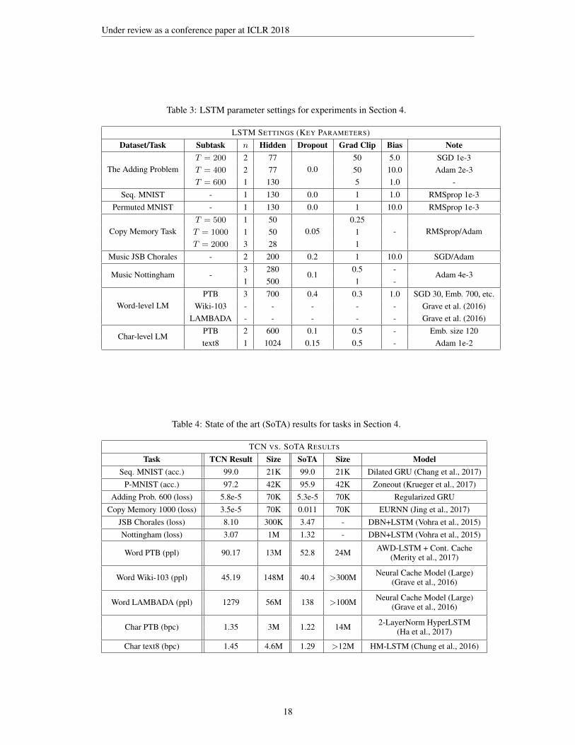
Table 3: LSTM parameter settings for experiments in Section 4.

LSTM SETTINGS (KEY PARAMETERS)Dataset/Task Subtask n Hidden Dropout Grad Clip Bias Note

The Adding ProblemT = 200 2 77

0.050 5.0 SGD 1e-3

T = 400 2 77 50 10.0 Adam 2e-3T = 600 1 130 5 1.0 -

Seq. MNIST - 1 130 0.0 1 1.0 RMSprop 1e-3Permuted MNIST - 1 130 0.0 1 10.0 RMSprop 1e-3

Copy Memory TaskT = 500 1 50

0.050.25

- RMSprop/AdamT = 1000 1 50 1T = 2000 3 28 1

Music JSB Chorales - 2 200 0.2 1 10.0 SGD/Adam

Music Nottingham -3 280

0.10.5 -

Adam 4e-31 500 1 -

Word-level LMPTB 3 700 0.4 0.3 1.0 SGD 30, Emb. 700, etc.

Wiki-103 - - - - - Grave et al. (2016)LAMBADA - - - - - Grave et al. (2016)

Char-level LMPTB 2 600 0.1 0.5 - Emb. size 120text8 1 1024 0.15 0.5 - Adam 1e-2

Table 4: State of the art (SoTA) results for tasks in Section 4.

TCN VS. SOTA RESULTS

Task TCN Result Size SoTA Size ModelSeq. MNIST (acc.) 99.0 21K 99.0 21K Dilated GRU (Chang et al., 2017)

P-MNIST (acc.) 97.2 42K 95.9 42K Zoneout (Krueger et al., 2017)Adding Prob. 600 (loss) 5.8e-5 70K 5.3e-5 70K Regularized GRU

Copy Memory 1000 (loss) 3.5e-5 70K 0.011 70K EURNN (Jing et al., 2017)JSB Chorales (loss) 8.10 300K 3.47 - DBN+LSTM (Vohra et al., 2015)Nottingham (loss) 3.07 1M 1.32 - DBN+LSTM (Vohra et al., 2015)

Word PTB (ppl) 90.17 13M 52.8 24M AWD-LSTM + Cont. Cache(Merity et al., 2017)

Word Wiki-103 (ppl) 45.19 148M 40.4 >300M Neural Cache Model (Large)(Grave et al., 2016)

Word LAMBADA (ppl) 1279 56M 138 >100M Neural Cache Model (Large)(Grave et al., 2016)

Char PTB (bpc) 1.35 3M 1.22 14M 2-LayerNorm HyperLSTM(Ha et al., 2017)

Char text8 (bpc) 1.45 4.6M 1.29 >12M HM-LSTM (Chung et al., 2016)

18


C THE EFFECT OF FILTER SIZE AND RESIDUAL BLOCK ON TCN

(a) Different k on Copy MemoryTask

(b) Different k on P-MNIST (c) Different k on PTB (word)

(d) Residual on Copy Memory Task (e) Residual on P-MNIST (f) Residual on PTB (word)

Figure 8: Controlled experiments that examine different components of the TCN model

In this section we briefly study, via controlled experiments, the effect of filter size and residualblock on the TCN’s ability to model different sequential tasks. Figure 8 shows the results of thisablative analysis. We kept the model size and the depth of the networks exactly the same within eachexperiment so that dilation factor is controlled. We conducted the experiment on three very differenttasks: the copy memory task, permuted MNIST (P-MNIST), as well as word-level PTB languagemodeling.

Through these experiments, we empirically confirm that both filter sizes and residuals play importantroles in TCN’s capability of modeling potentially long dependencies. In both the copy memory andthe permuted MNIST task, we observed faster convergence and better result for larger filter sizes(e.g. in the copy memory task, a filter size k ≥ 3 led to only suboptimal convergence). In word-levelPTB, we find a filter size of k = 3 works best. This is not a complete surprise, since a size-k filteron the inputs is analogous to a k-gram model in language modeling.

Results of control experiments on the residual function are shown in Figure 8d, 8e and 8f. In allthree scenarios, we observe that the residual stabilizes the training by bringing a faster convergenceas well as better final results, compared to TCN with the same model size but no residual block.

19


D EXPERIMENTS: GATING MECHANISM ON TCN

One component that has shown to be effective in adapting a TCN to language modeling is the gatingmechanism within the residual block, which was used in works such as Dauphin et al. (2017). Inthis section, we empirically evaluate the effects of adding gated units to TCN.

We replace the ReLU within the TCN residual block with a gating mechanism, represented byan elementwise product between two convolutional layers, with one of them also passing througha sigmoid function σ(x)5. Prior works such as Dauphin et al. (2017) has used similar gating tocontrol the path through which information flows in the network, and achieved great performanceon language modeling tasks.

Table 5: TCN with Gating Mechanism within Residual Block.

RELU TCN VS. GATED TCN RESULTS

Task TCN TCN + GatingSeq. MNIST (acc.) 99.0 99.0

P-MNIST (acc.) 97.2 96.9Adding Prob. 600 (loss) 5.8e-5 5.6e-5

Copy Memory 1000 (loss) 3.5e-5 0.00508JSB Chorales (loss) 8.10 8.13Nottingham (loss) 3.07 3.12

Word PTB (ppl) 90.17 88.91

Char PTB (bpc) 1.35 1.343

Char text8 (bpc) 1.45 1.48

Through these comparisons, we notice that gating components do further improve the TCN resultson certain language modeling datasets like PTB, which agrees with prior works. However, we do notobserve such benefits to exist in general on sequence prediction tasks, such as on polyphonic musicdatasets, and those simpler benchmark tasks requiring more long-term memories. For example, onthe copy memory task with T = 1000, we find that gating mechanism deteriorates the convergenceof TCN to a suboptimal result that is only slightly better than random guess.

5Note that this introduces approximately twice as many convolutional layers than in generic TCN describedin section 3. In Table 5, we keep the number of parameters for both architecture at about the same size

20

convolutional sequence modeling revisited

Documents