Federal Reserve Bank of Minneapolis Research Department Staff Report 511 May 2015

Coordination and Crisis in Monetary Unions Mark Aguiar

Princeton University Manuel Amador

Federal Reserve Bank of Minneapolis Emmanuel Farhi

Harvard University Gita Gopinath

Harvard University ABSTRACT __________________________________________________________________________________

We study fiscal and monetary policy in a monetary union with the potential for rollover crises in sover-eign debt markets. Member-country fiscal authorities lack commitment to repay their debt and choose fis-cal policy independently. A common monetary authority chooses inflation for the union, also without commitment. We first describe the existence of a fiscal externality that arises in the presence of limited commitment and leads countries to over-borrow; this externality rationalizes the imposition of debt ceil-ings in a monetary union. We then investigate the impact of the composition of debt in a monetary union, that is the fraction of high-debt versus low-debt members, on the occurrence of self-fulfilling debt crises. We demonstrate that a high-debt country may be less vulnerable to crises and have higher welfare when it belongs to a union with an intermediate mix of high- and low-debt members, than one where all other members are low-debt. This contrasts with the conventional wisdom that all countries should prefer a union with low-debt members, as such a union can credibly deliver low inflation. These findings shed new light on the criteria for an optimal currency area in the presence of rollover crises. Keywords: Debt crisis; Coordination failures; Monetary union; Fiscal policy JEL classification: E4, E5, F3, F4 _____________________________________________________________________________________________

*Corresponding author: Gita Gopinath, Littauer Center 206, 1805 Cambridge Street, Cambridge, MA 02138, USA. Email: gopinath@harvard.edu. Tel: 617-495-8161. Fax: 617-495-8570. We thank Cristina Arellano, Patrick Kehoe, Enrique Mendoza, Tommaso Monacelli, Helene Rey, and seminar participants at several places for useful com-ments. We also thank Ben Hebert for excellent research assistance. Manuel Amador acknowledges support from the NSF (award number 0952816). The views expressed herein are those of the authors and not necessarily those of the Federal Reserve Bank of Minneapolis or the Federal Reserve System.

1 Introduction

Monetary unions are characterized by centralized monetary policy and decentralized fiscal

policy. The problems associated with stabilizing the impact on welfare of asymmetric shocks

across countries with a common monetary policy have been studied in depth starting with

the seminal work of Mundell (1961) on optimal currency areas. The ongoing Euro crisis has,

however, brought to the forefront a novel set of issues regarding welfare of countries in a

monetary union with asymmetric debt levels that are subject to rollover risk in sovereign

debt markets. To study these issues we provide a framework that describes the impact of

centralized monetary policy and decentralized fiscal policy on debt dynamics and exposure

to self-fulfilling debt crises. This analysis sheds new light on the criteria for an optimal

currency area in the presence of rollover crises.1

The environment consists of individual fiscal authorities that choose how much to con-

sume and borrow by issuing nominal bonds. A common monetary authority chooses inflation

for the union, taking as given the fiscal policy of its member countries. Both fiscal and mon-

etary policy is implemented without commitment. The lack of commitment on fiscal policy

raises the possibility of default. The lack of commitment on monetary policy makes the

central bank vulnerable to the temptation to inflate away the real value of its members’

nominal debt. In choosing the optimal policy ex post, the monetary authority trades off the

distortionary costs of inflation against the fiscal benefits of debt reduction. Lenders recognize

this temptation and charge a higher nominal interest rate ex ante, making ex post inflation

self-defeating.2

The joint lack of commitment and coordination gives rise to a fiscal externality in a mon-

etary union. The monetary authority’s incentive to inflate depends on the aggregate value of

debt in the union. Each country in the union ignores the impact of its borrowing decisions

on the evolution of aggregate debt and hence on inflation. We compare this to the case of a

small open economy where the fiscal and monetary authority coordinate on decisions while

maintaining the assumption of limited commitment. We show that a monetary union leads

to higher debt, higher long-run inflation and lower welfare. While coordination eliminates

the fiscal externality, it does not replicate the full-commitment outcome. Full commitment

in monetary policy gives rise to the first best level of welfare, with or without coordination

on fiscal policy. These two cases allow us to decompose the welfare losses in the monetary

union due to lack of coordination versus lack of commitment. The presence of this fiscal

1For a survey on optimal currency areas see Silva and Tenreyro (2010).2Barro and Gordon (1983) in a seminal paper demonstrate the time inconsistency of monetary policy and

the resulting inflationary bias.

2

externality rationalizes the imposition of debt ceilings in a monetary union.3

In this context of debt overhang onto monetary policy, we explore the composition of

the monetary union. In particular, we consider a union comprised of high- and low-debt

economies, where the groups differ by the level of debt at the start of the monetary union.

Consider first the case without rollover crises, that is there is no coordination failure among

lenders in rolling over maturing debt. While inflation is designed to alleviate the real debt

burden of the members, all members, regardless of debt level, would like to be part of a low-

debt monetary union. This is because in a high-debt monetary union the common monetary

authority is tempted to inflate to provide debt relief ex post but the lenders anticipate this

and the higher inflation is priced into interest rates ex ante. Consequently, the members

in a union obtain no debt relief and only incur the deadweight cost of inflation. A low-

debt monetary union therefore better approximates the full-commitment allocation of low

inflation and correspondingly low nominal interest rates. High-debt members recognize they

will roll over their nominal bonds at a lower interest rate in such a union, thereby benefiting

from joining a low-debt monetary union. This agreement on membership criteria, however,

does not survive the possibility of rollover crises.

In particular, we consider equilibria in which lenders fail to coordinate on rolling over

maturing debt. This opens the door to self-fulfilling debt crises for members with high

enough debt levels. In this environment, there is a trade-off regarding membership criteria.

As in the no-crisis benchmark, a low-debt union can credibly promise low inflation, which

leads to low nominal interest rates and low distortions. However, in the presence of rollover

crises monetary policy not only should deliver low inflation in tranquil times but also serve

as a lender of last resort to address (and potentially eliminate) coordination failures among

lenders. The monetary authority of a union comprised mainly of low-debtors may be un-

willing to inflate in the event of a crisis, as such inflation benefits only the highly indebted

members at the expense of higher inflation in all members. That is, while low-debt member-

ship provides commitment to deliver low inflation in good times, it undermines the central

bank’s credibility to act as lender of last resort. Therefore, highly indebted economies prefer

a monetary union in which a sizeable fraction of members also have high debt, balancing

commitment to low inflation against commitment to act as a lender of last resort.

Importantly, the credibility to inflate in response to a crisis (an off-equilibrium promise)

may eliminate a self-fulfilling crisis without the need to inflate in equilibrium. This implica-

tion of the model is consistent with the events in the summer of 2012 when the announcement

3Debt ceilings on member countries are a feature of the Stability and Growth Pact in the eurozone. Similardebt ceilings exist on individual states in the U.S. Von Hagen and Eichengreen (1996) provide evidence ofdebt constraints on sub-national governments in a large number of countries, each of which works like amonetary union.

3

by Mario Draghi that the European Central Bank (ECB) would do “whatever it takes” to

defend the euro sharply reduced the borrowing costs for Spain, Italy, Portugal, Greece and

Ireland.4 This put the brakes on what arguably looked like a self-fulfilling debt crisis in the

eurozone, without the ECB having to buy any distressed country debt.5

One way to interpret these findings is to consider the decision of an indebted country to

join a monetary union or to have independent control over its monetary policy. In the absence

of rollover crises the country is best served by joining a monetary union with low aggregate

debt, as in such a union the monetary authority will deliver low inflation. This is the classic

argument for joining a union with a monetary authority that has greater credibility to keep

inflation low.6 By contrast, in the presence of self-fulfilling rollover crises, the country can

be better off by joining a monetary union with intermediate level of aggregate debt, as this

reduces its vulnerability to self-fulfilling crises compared to a union with low aggregate debt.

Our analysis therefore provides a new consideration in the design of optimal currency areas;

namely, eliminating self-fulfilling debt crises.7

Importantly, inflation credibility can be influenced endogenously through the debt com-

position of the monetary union. These findings shed new light on the criteria for an optimal

currency area and relates to the literature on institutional design for monetary policy. Rogoff

(1985b) highlighted the virtues of delegating monetary authority to a central banker whose

objective function can differ from society’s, so as to gain inflation credibility. Implement-

ing such delegation however may be difficult if society disagrees with the central banker’s

objectives. Here we demonstrate how debt characteristics of monetary union members en-

dogenously impact the inflation credibility of the monetary authority.

The rest of the paper is structured as follows. Section 2 places our paper in the context

of the existing literatures. Section 3 presents the model in an environment without rollover

crises. It characterizes the fiscal externality in a monetary union. Section 4 analyzes the

case with rollover crises. Section 5 discusses the implications for the optimal composition

4De Grauwe (2011) emphasizes the importance of the lender of last resort role for the ECB.5The ECB announcement in 2012 was accompanied by the setting up of an Outright Monetary Trans-

actions facility to purchase distressed country debt. This intervention brought down spreads on distressedcountry debt without the ECB actually buying any such debt (which is an important difference from thesubsequent 2015 monetary accommodation in the form of a Quantitative Easing program involving euro areasovereign bonds). An alternative strategy would be for the core countries to promise fiscal transfers to theperiphery in the event of the crisis. The political economy constraints on engineering such transfers and theweak credibility of such promises make the ECB intervention more practical and credible, which is why wefocus on the latter.

6Alesina and Barro (2002) highlight the benefits of joining a currency union whose monetary authorityhas greater commitment to keeping inflation low in an environment where Keynesian price stickiness providesan incentive for monetary authorities to inflate ex post.

7To the extent that non-debtors suffer when co-unionists default, the non-debt members will also have anon-monotonic relationship between their welfare and the heterogeneity of the union.

4

of a union an indebted country is considering joining, and Section 6 concludes. Proofs and

some technical details are relegated to the appendix.

2 Literature Review

In this section we describe our contribution to the existing literature on optimal currency

areas. Our focus, unlike most of the existing literature, is on the interaction between inflation,

nominal debt dynamics and exposure to self-fulfilling debt crises in monetary unions.

A main finding of our analysis, as previously described, is that when subject to rollover

risk an indebted country can be better off joining a monetary union with intermediate level

of aggregate debt as compared to one with low aggregate debt. The optimal currency area

literature has emphasized the benefits to a country of joining a union that is “similar” to

itself in the context of Keynesian macro stabilization. Our criterion for optimal currency

areas also highlights that a country with high debt can be better off by joining a union that

has similar high-debtors as it then receives the benefit of monetary policy intervention in

the event of a rollover crisis.

However, there are two important reasons our criterion differs from the existing literature.

First, there is a limit to the benefits of similarity in our environment. A high-debt country

can be worse off by joining a union where everyone else is like itself as compared to one where

only an intermediate number of countries are like itself. This is because in the former case

the common monetary authority is tempted to inflate at all times, generating high inflation

in normal times that in turn makes it hard to generate surprise inflation in crisis times.

Such a monetary authority is unable to generate state-contingent inflation and is therefore

not successful in using inflation to prevent a rollover crisis. A high-debt country in this

case experiences the cost of high inflation without escaping a rollover crisis. This lowers

its welfare compared to joining a union with an intermediate level of high-debtors. This

contrasts with the Keynesian macro stabilization argument for symmetry in the literature

where welfare always increases with greater similarity.

Second, despite heterogeneity across countries in debt levels, active monetary intervention

to help high debtors does not necessarily make low debt countries worse off. This is because

the threat to inflate in response to a crisis is an off-equilibrium threat that prevents a

rollover crisis from occurring and therefore the higher inflation is not actually experienced.

This intervention is similar to the “Draghi put” whereby a crisis was averted by announcing

the ECB’s intention to buy sovereign bonds in the event of a crisis without having to buy any

sovereign debt in equilibrium. This again differs from the standard symmetry argument in

the literature where monetary policy interventions are equilibrium phenomena and therefore

5

trade-offs necessarily exist.

The other contribution relates to the fiscal externality in a monetary union. The combi-

nation of time inconsistency in monetary policy and of decentralized fiscal policy gives rise

to a fiscal externality in a monetary union. Fiscal externalities have indeed been previously

described in the literature, specifically in the important contributions of Chari and Kehoe

(2007) and Chari and Kehoe (2008) who describe the role of commitment in eliminating the

fiscal externality.8 We differ from these papers in that we demonstrate the separate role of

lack of coordination among fiscal authorities and monetary authority, and of lack of com-

mitment, in affecting inflation, debt dynamics and welfare in a monetary union. The lack

of coordination is a defining feature of monetary unions and so to isolate the role it plays

in impacting welfare we contrast the solution to the case where decision making is coor-

dinated but commitment is still lacking. Then we add in the role of lack of commitment.

We therefore decompose the welfare losses relative to the first best that arise from lack of

coordination and that which arises from lack of commitment.

In other literature Beetsma and Uhlig (1999) provide an argument for debt ceilings in

a monetary union that arise from political economy constraints, namely short-sighted gov-

ernments. Dixit and Lambertini (2001) and Dixit and Lambertini (2003) examine the im-

plications for output and inflation in a monetary union where fiscal policy is decentralized

and monetary policy is centralized, allowing for the authorities to have conflicting goals for

output and inflation. Cooper et al. (2014) and Cooper et al. (2010) examine the interaction

between fiscal and monetary policy in a monetary union including exploring the incentives

for a monetary bailout in the presence of regional debt. Araujo et al. (2012) consider some

implications of currency denomination of debt in the presence of self-fulfilling crises.

There exists an important literature jointly analyzing fiscal and monetary policies in

a monetary union in the presence of New Keynesian frictions such as for example Beetsma

and Jensen (2005), Gali and Monacelli (2008), Ferrero (2009) and Farhi and Werning (2013).

Separately Rogoff (1985a) analyzes coordination and commitment of monetary policies in

the context of a model with nominal rigidities. The focus of our paper differs from this

literature as it is on debt, inflation and crises.

8Velasco (2000) describes an interesting fiscal externality that arises in a “tragedy of commons” environ-ment where multiple groups/state governments share a common fiscal resource.

6

3 Model

3.1 Environment

There is a measure-one continuum of small open economies, indexed by i ∈ [0, 1], that form

a monetary union. Fiscal policy is determined independently at the country-level, while

monetary policy is chosen by a single monetary authority. In this section we consider the

case where economies are not subject to rollover risk, that is lenders can commit to roll over

debt. We introduce rollover risk in section 4.

Time is continuous and there is a single traded consumption good with a world price

normalized to one. Each economy is endowed with yi = y units of the good each period that

is assumed to be constant. The domestic currency price at time t is denoted Pt = P (t) =

P (0)e´ t0 π(t)dt, where π(t) denotes the rate of inflation at time t.9 The domestic-currency

price level is the same across member countries and its evolution is controlled by the central

monetary authority.10

Preferences Each fiscal authority has preferences over paths for consumption and inflation

given by:

U f =

ˆ ∞0

e−ρt (u (ci(t))− ψ(π(t))) dt. (Uf)

Utility over consumption satisfies the usual conditions, u′ > 0, u′′ < 0, limc↓0 u′(c) = ∞.

As the fiscal authority controls ci(t), u(c) is the relevant portion of the objective function

in terms of fiscal choices. The second term, ψ(π(t)) reflects the preferences of the fiscal

authority in each country over the inflation choices made by the central monetary authority.

This term captures in reduced form the distortionary costs of inflation borne by the individual

countries. For tractability purposes we assume ψ(π(t)) ≡ ψ0π(t) and we restrict the choice

of inflation to the interval π ∈ [0, π].

The monetary authority preferences are an equally-weighted aggregate over all the economies

9As we shall see, we assume that the monetary authority’s policy selects π(t) ≤ π < ∞, and so thedomestic price level is a continuous function of time. Moreover, we treat the initial price level P (0) asa primitive of the environment, which avoids complications arising from a large devaluation in the initialperiod. This is similar to bounding the initial capital levy in a canonical Ramsey taxation program. Thisalso speaks to the differences between our environment and the “fiscal theory of the price level.” In thatliterature, the initial price level adjusts to ensure that real liabilities equal a given discounted stream of fiscalsurpluses. In our environment, we take the initial price level as given and solve for the equilibrium path offiscal surpluses and inflation.

10For evidence of convergence in euro area inflation rates and price levels see Lopez and Papell (2012) andRogers (2001).

7

in the monetary union:

Um =

ˆ ∞0

e−ρt(ˆ

i

u (ci(t)) di− ψ(π(t))

)dt. (Um)

Bond Markets Each country i can issue a non-contingent nominal bond that must be

continuously rolled over. Denote Bi(t) the outstanding stock of country i’s debt, the real

value of which is denoted bi(t) ≡ Bi(t)P (t)

. We normalize the price of a bond to one in local

currency and clear the market by allowing the equilibrium nominal interest rate ri(t) to

adjust. Denoting country i’s consumption by ci(t), the evolution of nominal debt is given

by:

Bi(t) = P (t) (ci(t)− y) + ri(t)Bi(t),

which can be re-written in terms of real debt using the identity b(t)/b(t) = B(t)/B(t)−π(t)

as

bi(t) = ci(t)− y + (ri(t)− π(t)) bi(t).

The rate of change of the real debt is equal to the sum of the real trade deficit and the real

interest payment on the debt. The role of inflation in reducing the real payments on the

debt for a given nominal interest rate is evident from the constraint.

Bonds are purchased by risk-neutral lenders who behave competitively and have an op-

portunity cost of funds ρ, same as the countries’ discount rate. We ignore the resource

constraint of lenders as a group by assuming that the monetary union is small in world

financial markets (although each country is a large player in terms of its own debt). In par-

ticular, we assume that country i’s bond market clears as long as the expected real return

is ρ.

As we discuss in the next subsection, fiscal authorities cannot commit to repay loans. In

particular, at any moment T , a fiscal authority can default and pay zero. We assume that if

it defaults, it is punished by permanent loss of access to international debt markets plus a

loss of output given by the parameter χ. We also assume that when an individual country

makes the decision to default it is not excluded from the union. We let V (T ) represent the

continuation value after a default.

V (T ) =u((1− χ)y)

ρ−ˆ ∞T

e−ρ(t−T )ψ(π(t))dt. (1)

8

Note that the default payoff depends on union-wide inflation, but does not depend on the

amount of debt prior to default.11

In the above formulation, we distinguish outright default from implicit partial default

through inflation for a number of reasons. First, outright default in the present model is a

choice of the fiscal authorities, while inflation is chosen by the monetary authority. Second,

the model allows us to consider environments where the two costs of default are treated

differentily by market participants. For example, the period of high inflation during the

1970s in the U.S. and Western Europe lead to a reduction in the real value of outstanding

bonds; but the governments did not enter a renegotiation with creditors or lose access to

financial markets, as is typically the case during an outright default episode.

3.2 Symmetric Markov Perfect Equilibrium

We are interested in the equilibrium of the game between competitive lenders, individual

fiscal authorities, and a centralized monetary authority. In particular, we construct a Markov

perfect equilibrium in which each member country behaves symmetrically in terms of policy

functions. The payoff-relevant state variables are the outstanding amounts of nominal debt

issued by member countries and the aggregate price level. We can substitute the real value

of debt using the assumption that P (0) is given.

In general, the aggregate state is the distribution of bonds across all members of the

monetary union. We are interested in environments in which members differ in their debt

stocks, allowing us to explore potential disagreement among members regarding policy and

the optimal composition of the monetary union. On the other hand, tractability requires

limiting the dimension of the state variable. To this end, we consider a union comprised

of high and low debt countries in the initial period. Let η ∈ (0, 1] denote the measure of

high-debt economies, and denote this group H and the low-debt group L. For tractability,

we assume that there is no within-group heterogeneity; that is, bi(0) = bH(0) for all i ∈ Hand bj(0) = bL(0) for all j ∈ L, with bH(0) > bL(0).

We focus on equilibria with symmetric policy functions, and so the initial within-group

symmetry is preserved in equilibrium. It is useful to introduce the following notation. Let

b(t)H = 1η

´i∈H bi(t)di denote the mean debt stock of the high-debt group, and let similarly

b(t)L = 11−η

´i∈L bi(t)di denote the debt stock of the low-debt group. Let b = (bH , bL) denote

the vector of mean debt stocks in the two subgroups of members.

11There is limited well identified empirical evidence on the costs of sovereign default. Therefore we stayclose to the standard assumptions in the sovereign debt literature on the costs of default, including that costsare independent of the level of debt prior to default. See Aguiar and Amador (2014) for a recent survey ofthe sovereign debt literature.

9

Using this notation, the relevant state variable for an individual fiscal authority is the

triplet (b, bH , bL) = (b, b), where the first argument is the country’s own debt level and the

latter characterizes the aggregate state. Let C(b, b) denote the optimal policy function for

the representative fiscal authority in the symmetric equilibrium. The monetary authority’s

policy function is denoted Π(b), where we incorporate in the notation that monetary policy

is driven by aggregate states alone and does not respond to idiosyncratic deviations from

the symmetric equilibrium.

The individual fiscal authority faces an equilibrium interest rate schedule denoted r(b, b).

The interest rate depends on the first argument via the risk of default and the latter argument

via anticipated inflation. In the current environment we abstract from rollover crises and

focus on perfect-foresight equilibria. Lenders will not purchase bonds if default is perfectly

anticipated, and thus fiscal authorities will have debt correspondingly rationed. From the

lender’s perspective, the real return on government bonds absent default is r(b, b) − Π(b),

which must equal ρ in equilibrium.12 In the deterministic case, there is no interest rate

that supports bond purchases if the government will default. Let Ω ⊂ [0,∞) denote the

endogenous domain of debt stocks that can be issued in equilibrium.13

Each fiscal authority takes the inflation policy function of the monetary authority Π(b)

as given, as well as the consumption policy functions of the other members of the union,

which we distinguish using a tilde, C(b, b). Given an initial state (b, b) ∈ Ω×Ω×Ω = Ω3

and

facing an interest rate schedule r(b, b) and domain Ω, we can express the fiscal authority’s

12To expand on this break-even condition, consider a bond purchased in period t that matures in periodt+m and carries a fixed interest rate rt = r(b(t), b(t)). The nominal return of this bond is ertm. Equilibriumrequires that the real return per unit time is ρ:(

P (t)

P e(t+m)

)ertm = eρm,

where superscript e denotes equilibrium expectations. Taking logs of both sides, dividing by m, letting

m→ 0, and using the definition that πe(t) = limm↓0lnP e(t+m)−lnP (t)

m , gives the condition rt = ρ+ πe(t). Inequilibrium, πe(t) = Π(bH(t), bL(t)), which gives the expression in the text.

13More specifically, let D(b, b) denote the default policy function, with D(b, b) = 1 if the fiscal authoritydefaults and zero otherwise. The additive separability in U implies that the optimal default decision ofan idiosyncratic fiscal authority is independent of inflation, and hence aggregate debt. Therefore, Ω =b|D(b, b) = 0 does not depend on the aggregate states. The restriction that b ≥ 0 is not restrictive in ourenvironment, as no fiscal authority has an incentive to accumulate net foreign assets.

10

problem in sequential form. For any initial debt b ∈ Ω:

V (b, b) = maxc(t)

ˆ ∞0

e−ρt (u (c(t))− ψ0Π(b(t))) dt, (P1)

subject to

b(t) = c(t)− y + [r(b(t), b(t))− Π(b(t))]b(t) with b(0) = b

bj(t) = C(bj(t), b(t))− y + [r(bj(t), b(t))− Π(b(t))]bj(t), for j = H,L

b(t) ∈ Ω, t ≥ 0.

As we shall see, the equilibrium Ω defines the domain on which the government does not

default. Therefore, it is not restrictive to write the problem for b ∈ Ω under the premise

the government does not default. The equilibrium value of default given aggregate state b is

given by V (b) = u((1−χ)y)ρ−ψ0

´∞0e−ρtΠ(b(t))dt, where bj(t), j = H,L, follow the equilibrium

evolution equations stated above.

Note that the aggregate state enters the fiscal authority’s problem only through the

cost of inflation and the term r(b, b) − Π(b). The latter is equal to ρ in equilibrium. It

is therefore convenient to state the value of the fiscal authority net of inflation costs, V =

V + ψ0

´∞0e−ρtΠ(b(t))dt, which will be independent of the aggregate state:

V (b) = maxc(t)

ˆ ∞0

e−ρtu (c(t)) dt, (P1’)

subject to

b(t) = c(t)− y + ρb(t) with b(0) = b

b(t) ∈ Ω, t ≥ 0.

Let C(b) denote the associated policy function.

The monetary authority sets inflation π(t) in every period without commitment. The

decision of the monetary authority can be represented by a sequence problem where the

monetary authority takes the interest rate function r(b, b) and the representative fiscal au-

thority’s consumption function C(b) as a primitive of the environment. For any debt level

11

(bH , bL) ∈ Ω2

the monetary authority solves the following problem:

J(b) = maxπ(t)∈[0,π]

ˆ ∞0

e−ρt [ηu(C(bH(t))) + (1− η)u(C(bL(t)))− ψ0π(t))] dt, (P2)

subject to

bj(t) = C(bj(t)) + [r(bj(t), b(t))− π(t)]bj(t)− ywith bj(0) = bj for j = H,L.

Note that the monetary authority takes the equilibrium interest rate schedule r as given.

From the lenders’ break-even constraint, we have that r(bj, b) = ρ + πe, for j = H,L,

where πe is the lenders’ expectation of inflation. In this sense the monetary authority is

solving its problem taking inflationary expectations as a given. This is why the solution

to the sequence problem (P2) is time consistent; the monetary authority is not directly

manipulating inflationary expectations with its choice of inflation. In equilibrium, πe =

Π(b), but this equivalence is not incorporated into the monetary authority’s problem as

the central bank cannot credibly manipulate market expectations. This contrasts with the

full-commitment Ramsey problem in which the monetary authority commits to a path of

inflation at time zero and thereby selects market expectations. The solution to that problem

is to set π = 0 every period.

Before discussing the solution to the problem of the fiscal and monetary authorities, we

define our equilibrium concept as follows.

Definition 1. A symmetric Recursive Competitive Equilibrium (RCE) is an interest rate

schedule r and associated domain Ω; a fiscal authority value function V and associated policy

function C; and a monetary authority value function J and associated policy function Π, such

that:

(i) V is the value function for the solution to the fiscal authority’s problem (P1’) and C is

the associated policy function;

(ii) J is the value function for the solution to the monetary authority’s problem and Π is

the associated policy function for inflation;

(iii) Bond holders break even: r(b, b) = ρ+ Π(b) for all (b, b) ∈ Ω3;

(iv) V (b) ≥ V ≡ u((1−χ)y)ρ

for all b ∈ Ω.

The last condition imposes that default is never optimal in equilibrium. In the absence of

rollover risk, there is no uncertainty and any default would be inconsistent with the lender’s

12

break-even requirement. As we shall see, this condition imposes a restriction on the domain

of equilibrium debt levels. It also ensures that problem (P1’), which presumes no default, is

consistent with equilibrium. That is, by construction the constraint b(t) ∈ Ω in (P1’) ensures

that the government would never exercise its option to default in any equilibrium.

Equilibrium Allocations The fiscal authority’s equilibrium policy sets b = 0 and C(b) =

y − ρb for all b ∈ Ω. This follows straightforwardly because income is constant and the

discount rate is equal to the interest rate. The associated value function is V (b) = u(y−ρb)/ρ.

The equilibrium domain Ω can be determined from the condition V (b) ≥ V , which implies

the maximal Ω =[0, χy

ρ

].

Turning to the monetary authority, faced with the above fiscal policy functions and the

equilibrium r(bj, b) = ρ+ Π(b) its problem becomes:

J(b) = maxπ(t)∈[0,π]

ˆ ∞0

e−ρt [ηu(y − ρbH(t)) + (1− η)u(y − ρbL(t))− ψ0π(t))] dt,

subject to

bj(t) = [Π(b(t))− π(t)] bj(t), j = H,L,

where the constraint substitutes C(b) = y − ρb into the debt evolution equation in (P2).

Note that Π(b) in the above problem represents the lenders’ equilibrium expectations, which

the monetary authority takes as given when choosing current inflation.

The associated Hamilton-Jacobi-Bellman equation is:

ρJ(b) = maxπ∈[0,π]

ηu(y − ρbH) + (1− η)u(y − ρbL)− ψ0π + (Π(b)− π)∇J(b) · b′,

wherever ∇J(b) =(

∂J∂bH

, ∂J∂bL

)exists. The first order condition with respect to π implies the

policy function satisfies:

Π(b) =

0 if ψ0 > −∇J(b) · b′,∈ [0, π] if ψ0 = −∇J(b) · b′,π if ψ0 < −∇J(b) · b′.

(2)

The inequalities that determine whether inflation is zero, maximal, or intermediate, have a

natural interpretation. The marginal disutility of inflation is ψ0. The perceived (ex post) gain

from inflation is a reduction in real debt levels conditional on consumption. This reduction

is proportional to the level of debt, and is translated into utility units via the terms ∇J .

Conditional on the optimal inflation policy, as well as the equilibrium behavior of lenders

13

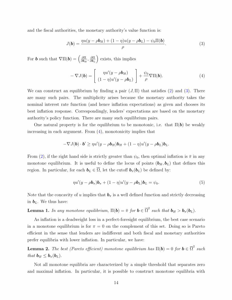
and the fiscal authorities, the monetary authority’s value function is:

J(b) =ηu(y − ρbH) + (1− η)u(y − ρbL)− ψ0Π(b)

ρ. (3)

For b such that ∇Π(b) =(∂Π∂bH

, ∂Π∂bL

)exists, this implies

−∇J(b) =

[ηu′(y − ρbH)

(1− η)u′(y − ρbL)

]+ψ0

ρ∇Π(b). (4)

We can construct an equilibrium by finding a pair (J,Π) that satisfies (2) and (3). There

are many such pairs. The multiplicity arises because the monetary authority takes the

nominal interest rate function (and hence inflation expectations) as given and chooses its

best inflation response. Correspondingly, lenders’ expectations are based on the monetary

authority’s policy function. There are many such equilibrium pairs.

One natural property is for the equilibrium to be monotonic, i.e. that Π(b) be weakly

increasing in each argument. From (4), monotonicity implies that

−∇J(b) · b′ ≥ ηu′(y − ρbH)bH + (1− η)u′(y − ρbL)bL.

From (2), if the right hand side is strictly greater than ψ0, then optimal inflation is π in any

monotone equilibrium. It is useful to define the locus of points (bH , bL) that defines this

region. In particular, for each bL ∈ Ω, let the cutoff bπ(bL) be defined by:

ηu′(y − ρbπ)bπ + (1− η)u′(y − ρbL)bL = ψ0. (5)

Note that the concavity of u implies that bπ is a well defined function and strictly decreasing

in bL. We thus have:

Lemma 1. In any monotone equilibrium, Π(b) = π for b ∈ Ω2

such that bH > bπ(bL).

As inflation is a deadweight loss in a perfect-foresight equilibrium, the best case scenario

in a monotone equilibrium is for π = 0 on the complement of this set. Doing so is Pareto

efficient in the sense that lenders are indifferent and both fiscal and monetary authorities

prefer equilibria with lower inflation. In particular, we have:

Lemma 2. The best (Pareto efficient) monotone equilibrium has Π(b) = 0 for b ∈ Ω2

such

that bH ≤ bπ(bL).

Not all monotone equilibria are characterized by a simple threshold that separates zero

and maximal inflation. In particular, it is possible to construct monotone equilibria with

14

Π(b) ∈ (0, π) for a non-trivial domain of b. These equilibria, however, are Pareto dominated

by the threshold equilibrium.

We collect the above in the following proposition:

Proposition 1. Define bπ(bL) from equation (5) and Ω =[0, χy

ρ

]. The following is the best

monotone equilibrium. For all (b, b) ∈ Ω3:

(i) Consumption policy functions:

C(b) = y − ρb;

(ii) Inflation policy function:

Π(b) =

0 if bH ≤ bπ(bL),

π if bH > bπ(bL);

(iii) Interest rate schedule:

r(b, b) =

ρ if bH ≤ bπ(bL),

ρ+ π if bH > bπ(bL);

(iv) Value functions:

V (b) =u(y − ρb)

ρ;

V (b, b) =

V (b) if bH ≤ bπ(bL),

V (b)− ψ0πρ

if bH > bπ(bL);

and J(b) = ηV (bH , b) + (1− η)V (bL, b).

The best monotone equilibrium is graphically depicted in figure 1. We do so for a given

bL and let bH vary along the horizontal axis, imposing the symmetry condition b = bH for

all high debtors. Given the symmetry of the environment, diagrams holding bH constant

and varying bL have similar shapes, but with thresholds defined by the inverse of bπ.

A prominent feature of this equilibrium is the discontinuity at bπ of the functions V

and J with respect to the aggregate state b. A small decrease in aggregate debt in the

neighborhood above bπ leads to a discrete jump in welfare. The lack of coordination between

fiscal and monetary authorities prevents the currency union from exploiting this opportunity,

15

as each fiscal authority takes the aggregate level of debt as given. We now discuss this “fiscal

externality” in greater detail.

3.3 Fiscal externalities in a monetary union

In this subsection, for expositional ease we assume all members of the monetary union have

the same level of debt. In particular, we set η = 1 and suppress bL in the notation. Let bπ

denote the solution to (5) when η = 1 (that is, u′(y − ρbπ)bπ = ψ0). In the next subsection,

we return to the case of heterogeneity to explore the extent of disagreement about policy

and composition of the monetary union.

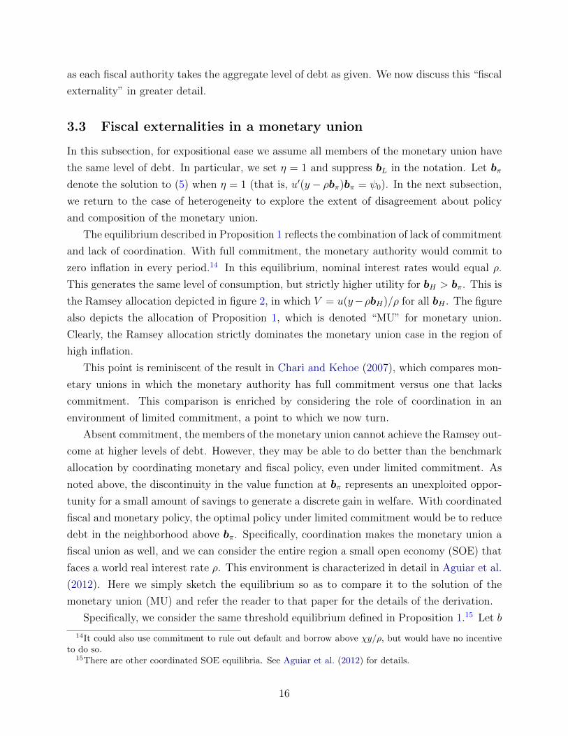
The equilibrium described in Proposition 1 reflects the combination of lack of commitment

and lack of coordination. With full commitment, the monetary authority would commit to

zero inflation in every period.14 In this equilibrium, nominal interest rates would equal ρ.

This generates the same level of consumption, but strictly higher utility for bH > bπ. This is

the Ramsey allocation depicted in figure 2, in which V = u(y−ρbH)/ρ for all bH . The figure

also depicts the allocation of Proposition 1, which is denoted “MU” for monetary union.

Clearly, the Ramsey allocation strictly dominates the monetary union case in the region of

high inflation.

This point is reminiscent of the result in Chari and Kehoe (2007), which compares mon-

etary unions in which the monetary authority has full commitment versus one that lacks

commitment. This comparison is enriched by considering the role of coordination in an

environment of limited commitment, a point to which we now turn.

Absent commitment, the members of the monetary union cannot achieve the Ramsey out-

come at higher levels of debt. However, they may be able to do better than the benchmark

allocation by coordinating monetary and fiscal policy, even under limited commitment. As

noted above, the discontinuity in the value function at bπ represents an unexploited oppor-

tunity for a small amount of savings to generate a discrete gain in welfare. With coordinated

fiscal and monetary policy, the optimal policy under limited commitment would be to reduce

debt in the neighborhood above bπ. Specifically, coordination makes the monetary union a

fiscal union as well, and we can consider the entire region a small open economy (SOE) that

faces a world real interest rate ρ. This environment is characterized in detail in Aguiar et al.

(2012). Here we simply sketch the equilibrium so as to compare it to the solution of the

monetary union (MU) and refer the reader to that paper for the details of the derivation.

Specifically, we consider the same threshold equilibrium defined in Proposition 1.15 Let b

14It could also use commitment to rule out default and borrow above χy/ρ, but would have no incentiveto do so.

15There are other coordinated SOE equilibria. See Aguiar et al. (2012) for details.

16

denote the debt level of the SOE, which is the only state variable. Re-using notation, let r(b)

be defined on Ω, and equal to ρ for b ≤ bπ and ρ+ π for b > bπ, where bπ is as defined above.

We now sketch how the centralized fiscal and monetary authority responds to this schedule,

and verify that it is indeed an equilibrium. We then contrast the resulting allocation with

that depicted in figure 1.

Faced with this schedule, the unified “SOE” government solves the following problem:

VE(b) = maxπ(t)∈[0,π],c(t)

ˆ ∞0

e−ρt(u(c(b(t))− ψ0π(t))dt, (P3)

subject to

b(t) = c(t) + (r(b(t))− π(t))b(t)− y, b(0) = b and b(t) ∈ Ω,

where the subscript E refers to the value for a small open economy. Unlike the problem in

the monetary union, fiscal and monetary policies are determined jointly in (P3). Therefore

the impact of debt choices on inflation is internalized by the single authority.

At points where the value function is differentiable, the Bellman equation is given by,

ρVE(b) = maxπ(t)∈[0,π],c(t)

u(c)− ψ0π + V

′

E(b) (c− y + (r(b)− π)b). (6)

The first order conditions are:

u′(c) = −V ′E(b),

π =

0 if ψ0 ≥ −V ′E(b)b = u′(c)b

π if ψ0 < u′(c)b.

The first condition is the familiar envelope condition that equates marginal utility of con-

sumption to the marginal disutility of another unit of debt. However, such a condition is

not satisfied by the monetary authority’s value function in the uncoordinated equilibrium,

as seen in equation (4). In the coordinated case, there is no disagreement between monetary

and fiscal authorities regarding the cost of another unit of debt. In particular, this provides

the incentive for the fiscal authority to reduce debt in the neighborhood above bπ in the

coordinated equilibrium.

In the region b ∈ [0, bπ], the SOE, like the benchmark, faces an interest rate of ρ and

finds it optimal to set c = y− ρb and π = 0. The consumption is optimal as the rate of time

preference equals the interest rate and the latter is optimal as, by definition, ψ0 ≤ u′(y−ρb)bfor b ≤ bπ. Thus π = 0 satisfies the first order condition for inflation on this domain.

The distinction between a SOE and the benchmark MU allocation becomes apparent

17

in the neighborhood above bπ. We start with the allocation at bπ. At this debt level,

VE = u(y − ρbπ)/ρ, which is the value achieved in the MU equilibrium. As in the MU

economy, in the neighborhood above bπ, a small open economy cannot credibly deliver zero

inflation, as ψ0 < u′(y − ρb) for b > bπ. However, by saving it can do better than the MU

allocation. Specifically, the SOE chooses CE(b) < y−ρb, where CE denotes the consumption

policy function of the coordinated fiscal policy, and thus b(t) < 0. At this consumption,

ψ0 > u′(CE), and so the associated inflation remains ΠE(b) = π, validating the jump in the

equilibrium interest rate.

In the neighborhood above bπ, the SOE can achieve the value V (bπ) by saving a small

amount. That is, the SOE value function will be continuous at bπ. As noted above, the

monetary union keeps debt constant in this neighborhood as the idiosyncratic fiscal authori-

ties do not internalize this potential jump in welfare from a small decrease in aggregate debt.

There is no such externality in the coordinated case.

The precise level of consumption in the neighborhood above bπ can be determined by

substituting in the envelope condition into (6) and using continuity of VE. In particular,

define cE ∈ (0, y − ρbπ) as the solution to:

u(y − ρbπ)− (u(cE)− ψ0π) = u′(cE) (y − cE − ρbπ) .

This consumption level satisfies the Bellman equation as we approach bπ from above. The

left-hand side is the jump in flow utility once bπ is reached. The right-hand side is the

marginal cost of reducing debt; that is, the marginal utility of consumption times −b.Along the trajectory to bπ there is no incentive for the government to tilt consumption,

as its effective real interest rate is ρ. That is, CE(b) = cE < y − ρbπ = CE(bπ) on a domain

(bπ, b∗), where the upper bound on this domain is given by y − cE = ρb∗, the debt level at

which cE no longer generates b(t) < 0. For debt above b∗, the government prefers not to

save towards bπ as the length of time required to reach this threshold is prohibitive.

Collecting the above points, we can characterize the SOE allocation, which is depicted in

figure 2 alongside the benchmark “MU” and Ramsey economies. For b = bH ≤ bπ, the SOE,

Ramsey, and MU economies are identical. For b = bH > b∗, the SOE and MU economies

are likewise identical, as the SOE economy finds it optimal to set b(t) = 0 despite having

high inflation, as in the benchmark. However, there is a difference for b = bH ∈ (bπ, b∗).

Continuity at bπ places the SOE value function strictly above the MU case; however, limited

commitment places SOE strictly below the Ramsey welfare. More specifically, from the

envelope condition, the SOE’s flat consumption policy function (panel b) is associated with

a constant V ′E(b); that is, VE is linear on (bπ, b∗). Moreover, this value function is continuous,

18

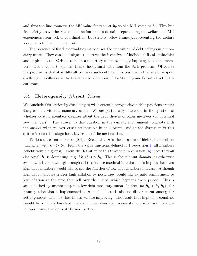
and thus the line connects the MU value function at bπ to the MU value at b∗. This line

lies strictly above the MU value function on this domain, representing the welfare loss MU

experiences from lack of coordination, but strictly below Ramsey, representing the welfare

loss due to limited commitment.

The presence of fiscal externalities rationalizes the imposition of debt ceilings in a mon-

etary union. They can be designed to correct the incentives of individual fiscal authorities

and implement the SOE outcome in a monetary union by simply imposing that each mem-

ber’s debt is equal to (or less than) the optimal debt from the SOE problem. Of course

the problem is that it is difficult to make such debt ceilings credible in the face of ex-post

challenges—as illustrated by the repeated violations of the Stability and Growth Pact in the

eurozone.

3.4 Heterogeneity Absent Crises

We conclude this section by discussing to what extent heterogeneity in debt positions creates

disagreement within a monetary union. We are particularly interested in the question of

whether existing members disagree about the debt choices of other members (or potential

new members). The answer to this question in the current environment contrasts with

the answer when rollover crises are possible in equilibrium, and so the discussion in this

subsection sets the stage for a key result of the next section.

To do so, we consider η ∈ (0, 1). Recall that η is the measure of high-debt members

that enter with bH > bL. From the value functions defined in Proposition 1, all members

benefit from a higher bπ. From the definition of this threshold in equation (5), note that all

else equal, bπ is decreasing in η if bπ(bL) > bL. This is the relevant domain, as otherwise

even low debtors have high enough debt to induce maximal inflation. This implies that even

high-debt members would like to see the fraction of low-debt members increase. Although

high-debt members trigger high inflation ex post, they would like ex ante commitment to

low inflation at the time they roll over their debt, which happens every period. This is

accomplished by membership in a low-debt monetary union. In fact, for bL < bπ(bL), the

Ramsey allocation is implemented as η → 0. There is also no disagreement among the

heterogeneous members that this is welfare improving. The result that high-debt countries

benefit by joining a low-debt monetary union does not necessarily hold when we introduce

rollover crises, the focus of the next section.

19

4 Rollover Crises

We now enrich our setup to allow for rollover crises defined as a situation where lenders

may refuse to roll over debt. This can generate default in equilibrium, unlike the analysis of

section 3. The distinction between high and low debtors will be a central focus of the analysis.

As in the no-crisis equilibrium from the previous section, in the equilibrium described below,

countries that start with low enough debt have no debt dynamics; as we shall see, this is

no longer the case for high debtors. To simplify the exposition, we set bL = 0 and drop bL

from the notation, as this state variable is always static in the equilibria under consideration.

That is, b = bH is sufficient to characterize the aggregate state in the equilibria described

below.

To introduce rollover crises, we follow Cole and Kehoe (2000) and consider coordination

failures among creditors. That is, we construct equilibria in which there is no default if

lenders roll over outstanding bonds, but there is default if lenders do not roll over debt. In

continuous time with instantaneous bonds, failure to roll over outstanding bonds implies a

stock of debt must be repaid with an endowment flow. To allow some notion of maturity in a

tractable manner, we follow Aguiar et al. (2012) and assume that the debt contract provides

the fiscal authority with a “grace period” of exogenous length δ during which it can repay

the bonds plus accumulated interest at the interest rate originally contracted on the debt. If

it repays within the grace period it returns to the financial markets in good standing. If the

government fails to make full repayment within the grace period and defaults, it is punished

by permanent loss of access to international debt markets plus a loss of output given by the

parameter χ. We continue to assume that it is not excluded from the union.16

We construct a crisis equilibrium as follows. We first consider the fiscal authority’s

and monetary authority’s problems in the grace period when creditors refuse to roll over

outstanding debt. We compute the welfare of repaying the bonds within the grace period

and compare that to the welfare from outright default. This will allow us to determine

whether or not a rollover crisis is possible given the state. We then define the full problem

of the fiscal and monetary authorities under the threat of a rollover crisis and characterize

the equilibria.

16In what follows, we restrict the fiscal authority to have access to the grace period only when there is arollover crisis. However, this is without loss of generality, as the fiscal authority would never exercise thegrace period when it can roll over bonds. This property follows because all the equilibria we study havedeclining interest rates over time, and the fiscal authority would strictly prefer to roll over bonds at a lowerrate.

20

4.1 The Grace Period Problem

In this subsection, we characterize the equilibrium response to a rollover crisis. When con-

fronted with a crisis, the government can either repay the principal due, or default. We

characterize the value conditional on repayment in this subsection. Keep in mind, however,

that repayment will be an off-equilibrium occurrence. The goal of the section, therefore, is

to establish in which states default dominates repayment.

We continue our focus on symmetric equilibrium and thus characterize the problem for

an individual country with debt b and the remaining debtors having debt b. This will allow

us to establish the payoffs to the idiosyncratic deviation of an individual fiscal authority.

Low-debt countries start with zero debt and, as a result, their consumption is given by c = y

and their debt remains at zero. With zero debt they are not subject to rollover crises. We

therefore focus on high-debt countries.

We assume that when a fiscal authority is faced with a run on its debt, it cannot issue

new bonds to repay maturing bonds. As discussed above, the fiscal authority has the option

of repaying all debt within the grace period of length δ or defaulting. When making its

decision, the individual fiscal authority takes the policies of the other fiscal authorities and

the monetary authority as given. However, the payoff to repayment depends on these other

policies, which in turn depends on whether the other fiscal authorities are themselves subject

to a rollover crisis.

In the grace period problem, the government is obligated to repay the nominal balance

on or before date δ, with interest accruing over the grace period at the original contracted

rate r.17 To set notation, we normalize t = 0 at the start of the grace period. The fiscal

authority’s repayment problem depends on the amount of debt outstanding as well as the

contracted interest rate, r. Let s ≡ (b, r) denote these individual states. The repayment

problem also depends on the inflation policy of the central bank during the grace period,

which we denote by the function Π : [0, δ]→ [0, π].

17As in Aguiar et al. (2012) we impose the pari passu condition that all bond holders have equal standing;that is, the fiscal authority cannot default on a subset of bonds, while repaying the remaining bondholders.Therefore, the relevant state variable is the entire stock of outstanding debt at the time the fiscal authorityenters the grace period.

21

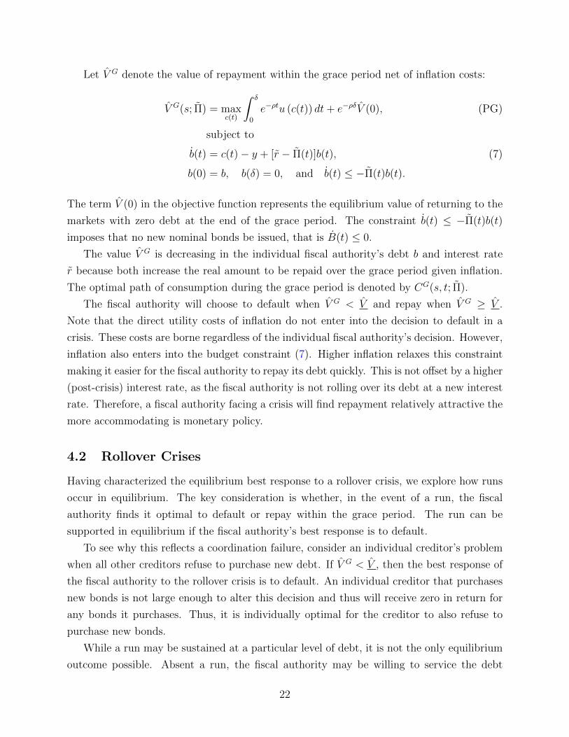
Let V G denote the value of repayment within the grace period net of inflation costs:

V G(s; Π) = maxc(t)

ˆ δ

0

e−ρtu (c(t)) dt+ e−ρδV (0), (PG)

subject to

b(t) = c(t)− y + [r − Π(t)]b(t), (7)

b(0) = b, b(δ) = 0, and b(t) ≤ −Π(t)b(t).

The term V (0) in the objective function represents the equilibrium value of returning to the

markets with zero debt at the end of the grace period. The constraint b(t) ≤ −Π(t)b(t)

imposes that no new nominal bonds be issued, that is B(t) ≤ 0.

The value V G is decreasing in the individual fiscal authority’s debt b and interest rate

r because both increase the real amount to be repaid over the grace period given inflation.

The optimal path of consumption during the grace period is denoted by CG(s, t; Π).

The fiscal authority will choose to default when V G < V and repay when V G ≥ V .

Note that the direct utility costs of inflation do not enter into the decision to default in a

crisis. These costs are borne regardless of the individual fiscal authority’s decision. However,

inflation also enters into the budget constraint (7). Higher inflation relaxes this constraint

making it easier for the fiscal authority to repay its debt quickly. This is not offset by a higher

(post-crisis) interest rate, as the fiscal authority is not rolling over its debt at a new interest

rate. Therefore, a fiscal authority facing a crisis will find repayment relatively attractive the

more accommodating is monetary policy.

4.2 Rollover Crises

Having characterized the equilibrium best response to a rollover crisis, we explore how runs

occur in equilibrium. The key consideration is whether, in the event of a run, the fiscal

authority finds it optimal to default or repay within the grace period. The run can be

supported in equilibrium if the fiscal authority’s best response is to default.

To see why this reflects a coordination failure, consider an individual creditor’s problem

when all other creditors refuse to purchase new debt. If V G < V , then the best response of

the fiscal authority to the rollover crisis is to default. An individual creditor that purchases

new bonds is not large enough to alter this decision and thus will receive zero in return for

any bonds it purchases. Thus, it is individually optimal for the creditor to also refuse to

purchase new bonds.

While a run may be sustained at a particular level of debt, it is not the only equilibrium

outcome possible. Absent a run, the fiscal authority may be willing to service the debt

22

as usual, paying off maturing bonds by issuing new bonds. Moreover, as discussed in the

previous subsections, the response of an individual fiscal authority depends on the actions of

the monetary authority, which in turn depends on the fraction η of other members in crisis.

To incorporate this multiplicity and interdependence in a tractable manner, we extend the

environment of Cole and Kehoe (2000), which considers the case of a small open economy.

Specifically, the equilibrium will define a region of the debt state space in which a fiscal

authority is vulnerable to a rollover crisis. Following Cole and Kehoe, we shall refer to this

region as the crisis region. To characterize a symmetric equilibrium, this region needs to be

defined over two dimensions– the own debt of an individual fiscal authority and the debt

of the representative fiscal authority. We hew as closely as possible to the single-country

case of Cole and Kehoe (2000) by considering a simple threshold bλ, such that an individual

debtor with debt b ∈ Ω is vulnerable to a crisis if b > bλ, regardless of the debt level of the

other members b. We shall refer to the set C ≡ b ∈ Ω|b > bλ as the “crisis zone,” and its

complement in Ω as the “safe zone.”

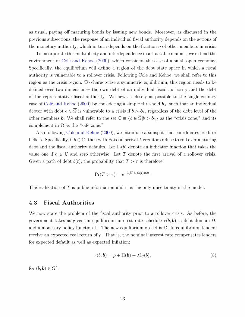
Also following Cole and Kehoe (2000), we introduce a sunspot that coordinates creditor

beliefs. Specifically, if b ∈ C, then with Poisson arrival λ creditors refuse to roll over maturing

debt and the fiscal authority defaults. Let IC(b) denote an indicator function that takes the

value one if b ∈ C and zero otherwise. Let T denote the first arrival of a rollover crisis.

Given a path of debt b(t), the probability that T > τ is therefore,

Pr(T > τ) = e−λ´ τ0 IC(b(t))tdt.

The realization of T is public information and it is the only uncertainty in the model.

4.3 Fiscal Authorities

We now state the problem of the fiscal authority prior to a rollover crisis. As before, the

government takes as given an equilibrium interest rate schedule r(b, b), a debt domain Ω,

and a monetary policy function Π. The new equilibrium object is C. In equilibrium, lenders

receive an expected real return of ρ. That is, the nominal interest rate compensates lenders

for expected default as well as expected inflation:

r(b, b) = ρ+ Π(b) + λIC(b), (8)

for (b, b) ∈ Ω2.

23

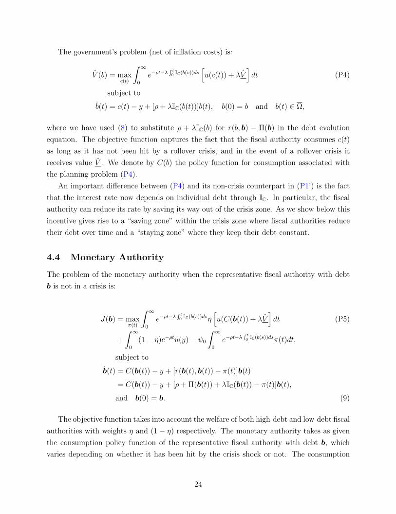
The government’s problem (net of inflation costs) is:

V (b) = maxc(t)

ˆ ∞0

e−ρt−λ´ t0 IC(b(s))ds

[u(c(t)) + λV

]dt (P4)

subject to

b(t) = c(t)− y + [ρ+ λIC(b(t))]b(t), b(0) = b and b(t) ∈ Ω,

where we have used (8) to substitute ρ + λIC(b) for r(b, b) − Π(b) in the debt evolution

equation. The objective function captures the fact that the fiscal authority consumes c(t)

as long as it has not been hit by a rollover crisis, and in the event of a rollover crisis it

receives value V . We denote by C(b) the policy function for consumption associated with

the planning problem (P4).

An important difference between (P4) and its non-crisis counterpart in (P1’) is the fact

that the interest rate now depends on individual debt through IC. In particular, the fiscal

authority can reduce its rate by saving its way out of the crisis zone. As we show below this

incentive gives rise to a “saving zone” within the crisis zone where fiscal authorities reduce

their debt over time and a “staying zone” where they keep their debt constant.

4.4 Monetary Authority

The problem of the monetary authority when the representative fiscal authority with debt

b is not in a crisis is:

J(b) = maxπ(t)

ˆ ∞0

e−ρt−λ´ t0 IC(b(s))dsη

[u(C(b(t)) + λV

]dt (P5)

+

ˆ ∞0

(1− η)e−ρtu(y)− ψ0

ˆ ∞0

e−ρt−λ´ t0 IC(b(s))dsπ(t)dt,

subject to

b(t) = C(b(t))− y + [r(b(t), b(t))− π(t)]b(t)

= C(b(t))− y + [ρ+ Π(b(t)) + λIC(b(t))− π(t)]b(t),

and b(0) = b. (9)

The objective function takes into account the welfare of both high-debt and low-debt fiscal

authorities with weights η and (1− η) respectively. The monetary authority takes as given

the consumption policy function of the representative fiscal authority with debt b, which

varies depending on whether it has been hit by the crisis shock or not. The consumption

24

of the low-debt fiscal authority is always equal to y. As long as the representative fiscal

authority is not in default, that is as long as it has not been hit by the crisis shock, the

monetary authority is tempted to inflate so as to reduce the real value of debt to be repaid,

thereby raising consumption and helping the fiscal authority exit the crisis zone. When the

representative fiscal authority is hit by the crisis shock and defaults, the monetary authority

sets inflation to zero as there is no benefit from inflating when there is zero debt. We denote

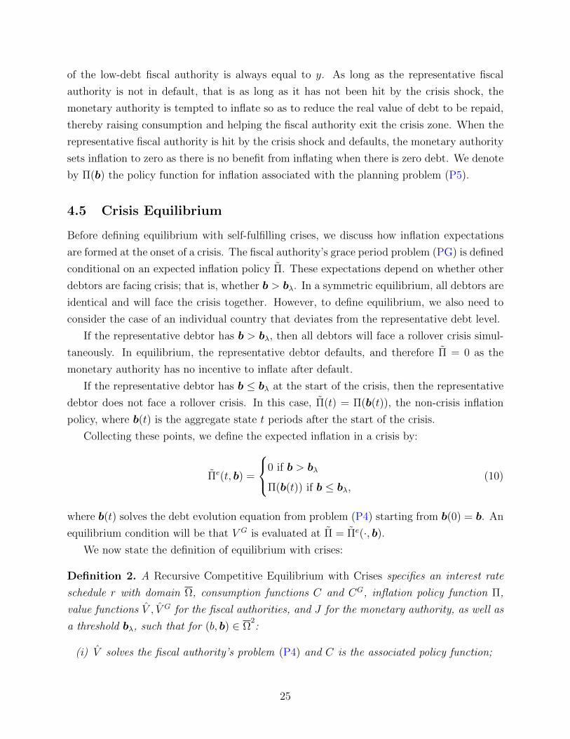
by Π(b) the policy function for inflation associated with the planning problem (P5).

4.5 Crisis Equilibrium

Before defining equilibrium with self-fulfilling crises, we discuss how inflation expectations

are formed at the onset of a crisis. The fiscal authority’s grace period problem (PG) is defined

conditional on an expected inflation policy Π. These expectations depend on whether other

debtors are facing crisis; that is, whether b > bλ. In a symmetric equilibrium, all debtors are

identical and will face the crisis together. However, to define equilibrium, we also need to

consider the case of an individual country that deviates from the representative debt level.

If the representative debtor has b > bλ, then all debtors will face a rollover crisis simul-

taneously. In equilibrium, the representative debtor defaults, and therefore Π = 0 as the

monetary authority has no incentive to inflate after default.

If the representative debtor has b ≤ bλ at the start of the crisis, then the representative

debtor does not face a rollover crisis. In this case, Π(t) = Π(b(t)), the non-crisis inflation

policy, where b(t) is the aggregate state t periods after the start of the crisis.

Collecting these points, we define the expected inflation in a crisis by:

Πe(t, b) =

0 if b > bλ

Π(b(t)) if b ≤ bλ,(10)

where b(t) solves the debt evolution equation from problem (P4) starting from b(0) = b. An

equilibrium condition will be that V G is evaluated at Π = Πe(·, b).

We now state the definition of equilibrium with crises:

Definition 2. A Recursive Competitive Equilibrium with Crises specifies an interest rate

schedule r with domain Ω, consumption functions C and CG, inflation policy function Π,

value functions V , V G for the fiscal authorities, and J for the monetary authority, as well as

a threshold bλ, such that for (b, b) ∈ Ω2:

(i) V solves the fiscal authority’s problem (P4) and C is the associated policy function;

25

(ii) V G solves the fiscal authority’s grace period problem (PG) and CG is the associated

policy function when r = r(b, b) and Π = Πe(·, b) defined in (10);

(iii) J solves the monetary authority’s problem (P5) and Π is the associated policy function;

(iv) Bond holders earn a real return ρ, that is r(b, b) = ρ+ Π(b) + λIC(b);

(v) V (b) ≥ V ; and

(vi) V G(b, r(b, b); Πe(·, b)) < V for b > bλ and all b ∈ Ω.

Condition (vi) ensures that a rollover crisis is consistent with equilibrium behavior.

Specifically, if a country is subject to a run on its debt, it will decide to default rather

than repay within the grace period. Given that the crisis region for a country does not

depend on the aggregate state, this must be true regardless of the representative country’s

debt position.

In what follows, we restrict attention to monotone equilibria where the inflation policy

follows a threshold rule (as was the case in the best monotone equilibrium without crises).

We will refer to these equilibria as monotone equilibria with thresholds. Among these, just

as in the case with no crisis, we analyze the one with the best possible inflation threshold.

We first characterize this equilibrium for a given bλ, and then discuss the determination of

the crisis threshold.

4.6 Equilibrium Policies

Fiscal Authority

The fiscal authority’s problem is stated in equation (P4). The value function satisfies the

following Hamilton-Jacobi-Bellman equation:

(ρ+ λIC(b))V (b) = maxc

u(c) + V ′(b)[(ρ+ λIC(b))b+ c− y] + λIC(b)V

, (11)

whenever V is differentiable at b, where we have used condition (iv) from the definition of

equilibrium to substitute out the equilibrium interest rate. The first order condition for the

fiscal authority is u′(c) = −V ′(b).

26

The solution V for b ∈ Ω is:18

V (b) =

u(y−ρb)

ρif b ≤ bλ,

V (bλ)− u′(cλ)(b− bλ) if bλ < b ≤ b∗

u(y−(ρ+λ)b)ρ+λ

+ λρ+λ

V if b∗ < b,

(12)

where cλ ∈ (0, y − (ρ+ λ)bλ) is the solution to:

(ρ+ λ)

ρu(y − ρbλ)−

(u(cλ) + λV

)= u′(cλ) (y − cλ − (ρ+ λ)bλ) , (13)

and b∗ = (y − cλ)/(ρ+ λ). The associated consumption policy function is:

C(b) =

y − ρb if b ≤ bλ

cλ if bλ < b ≤ b∗

y − (ρ+ λ)b if b∗ < b.

(14)

The consumption function implies the following for debt dynamics:

b =

−(ρ+ λ)(b∗ − b) if b ∈ (bλ, b∗)

0 otherwise.(15)

We now discuss why the solution takes this form.

If b /∈ C, the country is not vulnerable to a rollover crisis. With initial debt in the safe

zone, the solution to the fiscal authority’s problem is the same as that of problem (P1’)

described in the no-crisis equilibrium (Section 3). In particular, consumption maintains a

stationary debt level, C(b) = y− ρb. The individual fiscal authority has no incentive to save

in this region.

For b ∈ C, the fiscal authority does have an incentive to save. The fiscal authority can

eliminate the probability of default and the associated premium λ in its interest rate by

reducing debt to bλ. In contrast to reducing the incentive to inflate, which depends on

aggregate debt, there is no fiscal externality when it comes to reducing idiosyncratic default

risk.

The speed at which they save is governed by the Bellman equation (11). Specifically,

equation (13) is the Bellman equation evaluated as b approaches bλ from above, using the

knowledge of V (bλ) at the boundary of the safe zone plus the fact that V is continuous.

18See Aguiar et al. (2012) for the appropriate solution procedure to Hamilton-Jacobi-Bellman equationsof this type, including how to address points of non-differentiability.

27

Equation (13) determines the optimal consumption cλ in the neighborhood above bλ.

While the fiscal authority saves, it has no incentive to tilt consumption over time. That

is, it discounts at ρ + λ, which is the real interest rate on its debt in the crisis zone. In

particular, consumption is constant for a range of b as the fiscal authority saves towards

the safe zone. From the first order condition, u′(c) = −V ′(b), constant consumption implies

linearity in V .

Starting from high enough debt, the cost of saving to bλ is prohibitively high. In par-

ticular, at b∗ = (y − cλ)/(ρ + λ), the fiscal authority will not exit the crisis region in finite

time while consuming cλ. As a result, for b ≥ b∗ it prefers to remain in the crisis region

indefinitely. In this region, V takes the stationary-debt value when the real interest rate is

ρ+ λ and it faces a constant hazard λ of default.

Monetary Authority

The monetary authority’s problem is stated in (P5). The associated Hamilton-Jacobi-

Bellman equation, where J is differentiable, is:

(ρ+ λIC(b))J(b) = maxπ∈[0,π]

ηu(C(b)) + (1− η)u(y)− ψ0π (16)

+J ′(b)[(r(b)− π)b + C(b)− y] + λIC(b)J ,

where J ≡ ηV + (1 − η)u(y)ρ

is the monetary authority’s value post crisis. The first order

conditions imply that optimal inflation is zero if −J ′(b)b ≤ ψ0, and π otherwise.

By definition, the best equilibrium with thresholds sets inflation to zero over the largest

possible debt domain. We therefore look for the largest b such that −J ′(b)b ≤ ψ0. We

continue to denote the threshold for inflation as bπ, as in the non-crisis benchmark.

A useful insight in defining the inflation threshold is that in the interior of the domain

where inflation is zero, J ′(b) = ηV ′(b). To see this, from the solution to the fiscal authority’s

problem, we have b ≤ 0 in equilibrium. Therefore, if b ≤ bπ, inflation is always zero. This

implies that V (b) = V (b) for b ≤ bπ. Recall that the monetary authority’s value is the

weighted sum of V and the constant u(y)/ρ (when inflation is zero). It follows then that

J ′(b) = ηV ′(b) when b ≤ bπ.

The first order condition from the fiscal authority’s problem then implies that −J ′(b) =

ηu′ (C(b)) on the zero-inflation domain, where C is the fiscal authority’s policy function

given by (14). This leads to the following, which is proved in Appendix B:

28

Proposition 2. Conditional on bλ, the largest possible inflation threshold is such that:

bπ = supb

b ∈ Ω

∣∣∣∣u′ (C(b)) b ≤ ψ0

η

. (17)

Note that as C(b) is weakly decreasing in b and left continuous, definition (17) implies

that −J ′(b)b ≤ ψ0 for all b ≤ bπ. That is, on this domain zero inflation is the monetary

authority’s best response to the fiscal authority’s policy and expectations of zero inflation.

Appendix B demonstrates that zero inflation is not sustainable above bπ. Appendix B also

provides an analytical characterization of the monetary authority’s value function.

The associated inflation policy function is:

Π(b) =

0 if b ≤ bπ

π if bπ < b,(18)

and, the lenders’ break-even condition implies:

r(b, b) = ρ+ Π(b) + λIC(b). (19)

The preceding characterizes the equilibrium for a given crisis threshold bλ. We now turn

to the determination of this equilibrium threshold.

4.7 The Equilibrium Crisis Zone

There are many crisis equilibria corresponding to different thresholds bλ. Condition (vi) in

the equilibrium definition requires that V G < V in the crisis zone. However, it does not place

restrictions on the value of V G− V in the safe zone. Moreover, it does not place restrictions

on the off-equilibrium beliefs about Π if a crisis were to arrive when debtors are in the safe

zone. That is, if a crisis were to occur in the safe zone, at what Π do we evaluate V G?

We now propose beliefs that yield a unique threshold, and then motivate this equilibrium

selection.

Specifically, consider the scenario in which all debtors are facing a crisis, and the monetary

authority optimally sets inflation assuming that the debtors will repay within the grace

period. This provides crisis debtors with the maximal inflationary support for repayment

that is consistent with the monetary authority’s objective function. In particular, conditional

on the state s = (b, r) and the inflation expectations of the fiscal authorities Π, the monetary

authority solves the following grace period problem:

29

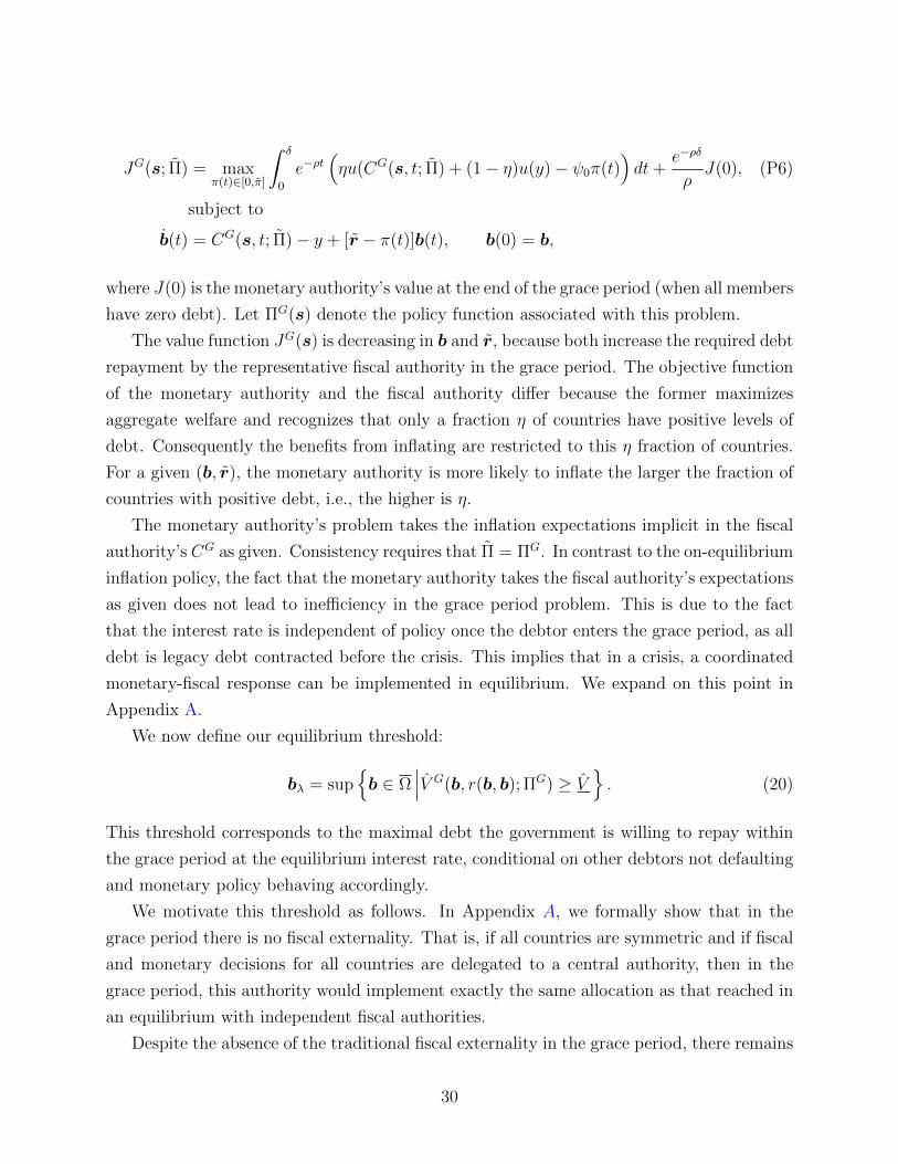
JG(s; Π) = maxπ(t)∈[0,π]

ˆ δ

0

e−ρt(ηu(CG(s, t; Π) + (1− η)u(y)− ψ0π(t)

)dt+

e−ρδ

ρJ(0), (P6)

subject to

b(t) = CG(s, t; Π)− y + [r − π(t)]b(t), b(0) = b,

where J(0) is the monetary authority’s value at the end of the grace period (when all members

have zero debt). Let ΠG(s) denote the policy function associated with this problem.

The value function JG(s) is decreasing in b and r, because both increase the required debt

repayment by the representative fiscal authority in the grace period. The objective function

of the monetary authority and the fiscal authority differ because the former maximizes

aggregate welfare and recognizes that only a fraction η of countries have positive levels of

debt. Consequently the benefits from inflating are restricted to this η fraction of countries.

For a given (b, r), the monetary authority is more likely to inflate the larger the fraction of

countries with positive debt, i.e., the higher is η.

The monetary authority’s problem takes the inflation expectations implicit in the fiscal

authority’s CG as given. Consistency requires that Π = ΠG. In contrast to the on-equilibrium

inflation policy, the fact that the monetary authority takes the fiscal authority’s expectations

as given does not lead to inefficiency in the grace period problem. This is due to the fact

that the interest rate is independent of policy once the debtor enters the grace period, as all

debt is legacy debt contracted before the crisis. This implies that in a crisis, a coordinated

monetary-fiscal response can be implemented in equilibrium. We expand on this point in

Appendix A.

We now define our equilibrium threshold:

bλ = supb ∈ Ω

∣∣∣V G(b, r(b, b); ΠG) ≥ V. (20)

This threshold corresponds to the maximal debt the government is willing to repay within

the grace period at the equilibrium interest rate, conditional on other debtors not defaulting

and monetary policy behaving accordingly.

We motivate this threshold as follows. In Appendix A, we formally show that in the

grace period there is no fiscal externality. That is, if all countries are symmetric and if fiscal

and monetary decisions for all countries are delegated to a central authority, then in the

grace period, this authority would implement exactly the same allocation as that reached in

an equilibrium with independent fiscal authorities.

Despite the absence of the traditional fiscal externality in the grace period, there remains

30

a “default externality.” The default externality arises because there may be more than

one equilibrium best response from the monetary union. If the fiscal authorities default,

the monetary authority will not inflate thus making repayment difficult. Conversely, an

alternative equilibrium response may exist in which fiscal authorities repay within the grace

period, aided by accommodative monetary policy.

While the default externality may be of interest in some contexts, it is not robust to a

straightforward coordination of beliefs among members of the monetary union. In Appendix

A, we show that if all countries are symmetric and if default, fiscal and monetary decisions

for all countries are delegated to a central authority, then faced with a rollover crisis, the

allocation implemented by this authority can also be reached when default and fiscal decisions

are made by independent fiscal authorities. That is, during the grace period, the monetary

union can achieve the single-decision-maker outcome by coordinating beliefs on the preferable

response.19

Our equilibrium selection imposes the requirement that if there exists an equilibrium

best response in which the monetary authority comes to the rescue of the fiscal authorities

in a crisis by generating high inflation, the fiscal authorities proceed as if they will be

rescued. This selection is appealing given the plausibility that beliefs within the union can

be coordinated in this way. Given these off-equilibrium beliefs, the threshold defined in (20)

generates the largest possible crisis zone.

The threshold defined in (20) is conditional on an equilibrium interest rate schedule.

Recall from the derivation of (17) that in any equilibrium, for b ≤ bλ we have J ′(b) =

ηV ′(b) = −ηu′ (y − ρb). Therefore, for b ≤ bλ, inflation will be zero if u′(y − ρb)b ≤ ψ0/η

and π otherwise. This implies that r(b, b) in equation (20) can be replaced by

ρ+ πIu′(y − ρb)b > ψ0/η, (21)

where Ix is the indicator function that takes the value one if x is true and zero otherwise.

We therefore can determine the boundary of the safe zone without using the equilibrium

interest rate schedule in the crisis zone.

Computing the equilibrium is therefore straightforward: The crisis threshold bλ is deter-

mined independently of bπ as explained in the previous paragraph. The crisis threshold is

sufficient to determine the fiscal authority’s policy function C(b), described in (14). With

C(b) in hand, bπ is determined from (17). The final step is to verify that these thresholds

indeed determine a monotone equilibrium. That is, for all b ≤ bπ, the monetary authority’s

19Note that this is very different than the fiscal externality in section 3.3. In that case, there was not aconsistent set of equilibrium beliefs that resolved the fiscal externality. Indeed, this result stems from thefact that there is no fiscal externality in the grace period as the interest rate on debt in arrears is constant.

31

best response is zero inflation, and similarly π is optimal for b > bπ.

Lemma 5 in Appendix B states the necessary conditions to ensure that the thresholds

above constitute an equilibrium.

4.8 Crisis Vulnerability and the Debt Distribution

A major goal of our analysis is to understand how the composition of the monetary union

affects the vulnerability to rollover crises. We do so by characterizing the dependence of bλ

on η. Figure 3 describes how the threshold bλ varies with the fraction of debtors η. The

vertical axis represents the candidate bλ and the horizontal axis is the parameter η.

The downward sloping line labelled R is a reference line that defines when the indicator

function in equation (21) is zero or one. Specifically, it traces the points such that u′(y −ρbλ)bλ = ψ0/η. If bλ lies strictly above this reference, then in equilibrium r(bλ, bλ) = ρ+ π.

If bλ lies weakly below this line, then r(bλ, bλ) = ρ. The line slopes down because as the

fraction of debtors increases, the monetary authority will start inflating at lower thresholds.

Below the R locus, we obtain bλ by substituting ρ for r in (20). As η → 0, the debtors

as a group are too small to affect monetary policy during a crisis. The monetary authority

therefore provides no assistance. As η increases, the monetary authority is willing to inflate

in the off-equilibrium event that a crisis arrives in the safe zone. This expands the safe zone,

and therefore the threshold bλ increases. This is the segment AB depicted in the figure.

Above the R locus, we obtain bλ by substituting ρ + π for r in (20). As V G is strictly

decreasing in r, this threshold is strictly below that when r = ρ, conditional on monetary

policy. As η increases, the safe zone is expanded as the monetary authority provides more

support in the grace period, while r does not change. This generates the upward sloping

segment CD.

At point B, the fiscal authority is indifferent to repayment versus default when r = ρ. At

point C, the fiscal authority is indifferent when r = ρ + π. There is an intermediate region

when the fiscal authority strictly prefers repayment when r = ρ, but strictly prefers default

when r = ρ+ π. As a result, the condition defining the threshold (20) traces the downward

sloping locus R along the segment BC. When bλ lies on R, then the crisis threshold bλ and

the equilibrium inflation threshold bπ are equivalent.

The threshold bλ is therefore non-monotonic in the fraction of debtors η. This reflects

the monetary authority’s tension between the on-equilibrium temptation to inflate and the

off-equilibrium promise to come to the aid in a crisis. At point B, we have the maximal

safe zone as we vary the fraction of debtors in the monetary union. This is the closest

approximation to a commitment not to inflate absent a crisis, but to optimally inflate in the

32

event of a crisis. For η below point B, the monetary authority can commit to low inflation

absent a crisis, but not credibly promise to act aggressively in the event of a crisis.

Conversely, along the segment BC, the threshold is determined by the debt level at which

the monetary authority begins to inflate absent a crisis. This is because, for debt levels above

R, the monetary authority cannot credibly promise low inflation. Along the segment BC,

the equilibrium interest rate is ρ. At that nominal interest rate, the union could support

more debt without becoming vulnerable to a crisis. However, it cannot support more debt

at a higher nominal interest rate. This is because the increase in interest rate reduces the

ability of the monetary authority to rescue debtors in a crisis. As a result, the threshold is

determined in this region by the indifference condition of the monetary authority regarding

equilibrium inflation.

The fact that the safe region is maximized at an interior η is relevant for our discussion

of optimal monetary union composition, which is contained in the next section.20

5 Optimal Composition of a Currency Union

In the case without self-fulfilling crises, a country with high debt is strictly better off when

every other member has low debt (η → 0), as discussed in Section 3. This composition of the

currency union endogenously lowers the benefit of inflation for the monetary authority thus

enabling it to deliver the commitment outcome of zero inflation. However, this conclusion

changes when countries are exposed to rollover risk. In this case a country with high debt

may be better off when there is an appropriate measure of high debtors. This reflects the

fact that the crisis region is minimized at an interior η in Figure 3.

To illustrate this, consider Figure 4. Each panel depicts an equilibrium value for two

different values of η. Case A refers to η = 0, which was point A in Figure 3. At point A, the

set of debtors is measure zero, and so equilibrium inflation is always zero. Case B refers to

the η at point B in Figure 3, which minimizes the crisis region. Recall that at point B, in

equilibrium bλ = bπ. A superscript denotes the respective case.

The figure has three panels. Panel (a) depicts the representative fiscal authority’s equi-

20In the model we do not allow for spillovers, say through a banking channel, on low debtors in the eventof a default by high debtors. If there exist such spillover costs it is reasonable to assume that this cost isstrictly increasing in the measure of defaulters. The presence of such costs does not alter any individual fiscalauthority’s decisions on consumption, borrowing or default. However, the monetary authority, which caresabout the union as a whole, will be more tempted to intervene in the event of a run on high-debtors becauseof the spillover effect on low-debtors. This will quantitatively impact the debt threshold and increase thesize of the safe zone relative to the case without spillovers. The non-monotonic relation between the debtthreshold and the fraction of high debtors in the union is maintained, except that it shifts up relative towhat is depicted in Figure 3.

33

librium value function V (b, b) inclusive of inflation costs, where we impose symmetry. Panel

(b) depicts the value net of inflation costs, V (b). Panel (c) depicts the inflation costs, V − V .

We start with panel (b). For b ≤ bAλ , V A(b) = V B(b) = u(y − ρb)/ρ. For b ∈ (bA, bB],

equilibrium A is vulnerable to a rollover crisis, while equilibrium B is safe. This reflects the

value of having the monetary authority stand ready to assist in the event of a crisis, which is

only credible if there are a sufficient number of debtors. On this domain, V A < V B. Recall

that in the neighborhood to the right of bλ, a fiscal authority will save. From the first order

condition u′(C(b)) = −V ′(b), this translates into a steeper slope for V A than for V B.

For b > bBλ , both A and B are vulnerable to a rollover crisis. However, by continuity, V B

continues to lie above V A. This reflects that less saving is required to eliminate the threat of

a crisis in case B. For b ≥ b∗B, debt is stationary in the crisis zone for both cases. Therefore,

V A = V B for b ≥ b∗B.

Turning to panel (c), we see that equilibrium A benefits from the commitment to low

inflation because it avoids inflation costs. For equilibrium A, inflation is always zero and

therefore V A − V A = 0. Recall that for case B, bBλ = bBπ . For b ≤ bπ, V B = V B as there

is no inflation in equilibrium. For b > bBπ , V B < V B, as inflation is strictly positive on this

domain. However, the present value of inflation costs is relatively small in the neighborhood

of bπ as the fiscal authority is saving towards bBπ = bBλ . The further b is above bBπ , the

greater the present value of costs. For b ≥ b∗B, the fiscal authority does not save, and

V B − V B = −ψ0π/(ρ+ λ).

Panel (a) sums these two figures. On the domain (bAλ , bBλ ) we have V B > V A, as both

have zero inflation costs but V B > V A due to the latter’s vulnerability to a crisis. There is

therefore a range of debt over which welfare is higher for a debtor in a monetary union with

a strictly positive measure of other debtors, compared to the case with no other debtors

(η = 0). This contrasts with the non-crisis benchmark equilibrium when η = 0 was the

optimal composition for the representative debtor. Note that for b ≤ bBπ , the non-debtors

are not worse off in a union with debtors, because inflation only happens off equilibrium.

However, in panel (b) we see that V A = V B for high enough b, while panel (c) implies a

strict welfare loss due to inflation in case B. This implies that V A > V B for high b, which

is depicted in panel (a) to the right of the intersection.

6 Conclusion

The ongoing eurozone crisis has brought to the forefront the inherent tensions in a monetary

union where individual countries have control over fiscal decisions but where monetary deci-

sions are made by a union wide monetary authority that maximizes welfare of the union as a

34

whole. It is a familiar argument that individual countries in a union are worse off when there

is limited synchronization in business cycles across countries, as a common monetary policy

for the union can be inconsistent with the needs of different countries. Here we highlight

another tension that arises when countries are subject to rollover risk in debt markets.

The monetary authority may be able to use surprise inflation to reduce the real value

of debt owed and thus eliminate a rollover crisis. Whether it will choose to do so and

whether it can effectively do so depends on the aggregate level of debt in the union. If the

aggregate level of debt in the union is low, the monetary authority will choose never to

inflate, neither in tranquil nor in crisis time. At the other extreme, if the aggregate debt

in the union is high, the monetary authority uses inflation all the time and consequently

fails to generate surprise inflation. On the other hand when there is an intermediate level

of aggregate debt the monetary authority chooses low inflation in normal times and high

inflation in crisis times, thus generating surprise inflation and helping to prevent a rollover

crisis. An indebted country in the union therefore gets no help from the monetary authority

in preventing self-fulfilling crises when everyone else in the union is as indebted as it is or

when no one in the union is like it. Greece is better off in a monetary union with members

like Germany, but not exclusively low debtors. The presence of other vulnerable debtors, like

Italy, Spain, Ireland, and Portugal, makes the ECB promised intervention in a crisis credible.

This composition gives debtors both low inflation and eliminates its exposure to self-fulfilling

crises. Importantly, this can take place without any loss of welfare to non-debtors if the use

of inflation is done off-equilibrium.21

What this analysis also highlights is that there is an intermediate range of debt at which

Greece may be better off with independent monetary policy than being a part of a monetary

union with only low debtors. This is because with independent monetary policy it is credibly

able to commit to the use of inflation in the event of a run on its debt and thereby can

eliminate a rollover crisis. If, however, Greek debt is high, it would be better off in a

monetary union with low debtors because it can benefit from the low inflation the union

is credibly able to offer without any loss in terms of exposure to rollover risk. This follows

because with high debt independent monetary policy results in high inflation in normal times

and therefore cannot generate surprise inflation in crisis times.

While we do not capture important aspects of the eurozone crisis, particularly the role of

the banking sector in amplifying the crisis, our analysis is consistent with the events following

the so-called Draghi put in the summer of 2012, when Draghi promised to do “whatever it

21We have described an environment where the debt of members of the union is held outside the union.In reality, as in the case of the eurozone, a significant fraction of the debt is held by members of the union.In our environment this would have similar effects to reducing η and therefore the incentive to inflate.

35

takes” to save the euro. This intervention caused spreads of troubled periphery country

bonds to decline sharply despite the absence of any actual purchase by the ECB of such

bonds (and importantly differs from the subsequent 2015 monetary accommodation in the

form of a Quantitative Easing program involving euro area sovereign bonds).

Clearly, debt crises disappear when a country’s debt is low enough. However, we demon-

strate the existence of a fiscal externality that limits individual countries’ incentive to reduce

their debt. This arises because they fail to internalize the impact of their debt on the union

monetary authority’s incentive to inflate. Consequently they end up with higher debt than

if they were an independent country with control over both fiscal and monetary policy. This

provides an argument for placing debt ceilings on countries in a monetary union.

36

A Fiscal and Default Externalities in Rollover Crises

In this appendix, we show that the coordinated fiscal-monetary response during the grace

period can be decentralized in our monetary union equilibrium in which the policies are set

by independent authorities. We first state the grace period problem for a single decision

maker:

V GE (b, r) = max

π(t)∈[0,π],c(t)

ˆ δ

0

e−ρt(ηu(c(t)) + (1− η)u(y)− ψ0π(t))dt+ e−ρδu(y)

ρ, (22)

subject to

b(t) = c(t) + (r − π(t))b(t)− y,b(t) ≤ −π(t)b(t),

b(0) = b, b(δ) = 0,

where as before r is the contracted interest rate at the start of the crisis (which is the

equilibrium rate of the decentralized monetary union). For this problem, consumption and

inflation are coordinated.

Let πE(t) be the optimal inflation policy from this problem. Now consider an individual

fiscal authority’s problem conditional on πE. This problem net of inflation costs is:

V G(b, r; πE) = maxc(t)

ˆ δ

0

e−ρtu(c(t)dt+ e−ρδu(y)

ρ, (23)

subject to

b(t) = c(t) + (r − πE(t))b(t)− y,b(t) ≤ −πE(t)b(t),

b(0) = b, b(δ) = 0.

It is clear that the optimal individual fiscal policy coincides with that from Problem (22).

That is, the unitary fiscal policy is the best response to πE in the monetary union equilibrium.

Similarly, πE is the monetary authority’s best response to this fiscal policy. Therefore, the

single-decision-maker policies can be sustained in the monetary union equilibrium.

This implies that there is no fiscal externality in the grace period problem. The key

difference between this problem and the equilibrium fiscal policy problem is that the interest

rate for the grace period is a constant; in particular, it is not a function of fiscal decisions.

37

Outside of the grace period (on the equilibrium path), fiscal authorities fail to internalize

the impact their individual debt choices have on the aggregate debt, and therefore have on

r(b, b).

Despite the absence of the traditional fiscal externality in the grace period, there remains

a “default externality.” The default externality arises because there may be more than

one equilibrium best response from the monetary union. If the fiscal authorities default,

the monetary authority will not inflate thus making repayment difficult. Conversely, an

alternative equilibrium response may exist in which fiscal authorities repay within the grace

period, aided by accommodative monetary policy.

While the default externality may be of interest in some contexts, it is not robust to a

straightforward coordination of beliefs among members of the monetary union. In particular,

since the solution to Problem (22) can be supported in the decentralized equilibrium, it is

reasonable that the monetary authority can coordinate beliefs on this outcome. That is, if

fiscal authorities believe that the monetary authority will help them during the grace period

by setting π = πE, they will only default if V G < V , where V G solves Problem (23). Note

that this is the same default criterion that would be used by a unified decision maker.

B Existence and Characterization of Monotone Equi-

libria

In this appendix, we characterize the monetary authority’s equilibrium value function and

associated inflation policy. We first consider an arbitrary monotone threshold equilibrium

and characterize the value function of the monetary authority that is implied by creditor

beliefs. That is, consider an equilibrium interest rate function r(b, b) defined by the crisis

threshold bλ defined by (20), an arbitrary inflation threshold bπ, and a domain Ω = [0, bmax]

that sets an upper bound on debt. The associated equilibrium beliefs are therefore Π(b) = 0

for b ≤ bπ and π otherwise. Lemma 3 derives the value function implied by this policy.

Lemma 4 establishes that bπ defined in equation (17) is an upper bound on the set of

possible equilibrium inflation thresholds. Finally, Lemma 5 establishes that the monetary

authority has no incentive to deviate from the policy implied by the threshold bπ. These

lemmas constitute the proof of Proposition 2 that states bπ is the threshold associated with

the best monotone equilibrium.

We establish these points assuming the borrowing limit bmax lies above the thresholds

bπ, bλ and b∗. This is without loss of generality in terms of establishing optimal monetary

policy as the location of the borrowing limit relative to these thresholds does not influence

38

the monetary authority’s problem on the interior of Ω. It is straightforward to then truncate

the monetary authority’s value and policy functions to the appropriate domain Ω = [0, bmax].

The next lemma characterizes the monetary authority’s value function conditional on the

triplet bλ, bπ, bmax. We discuss the key characteristics of the value function after the proof

of the lemma. For reference, recall that associated with any equilibrium is a consumption

policy function C(b) defined in (14) and characterized by cλ from (13) and the associated

b∗ = (y − cλ)/(ρ+ λ).

Lemma 3. In any monotone equilibrium with thresholds bλ, bπ and domain Ω = [0, bmax],

the monetary authority’s value function J satisfies

J(b) = ηV (b) + (1− η)u(y)

ρ−Ψ(b), (24)

where V is defined by (12) and Ψ(b) is:

(i) If bπ < bλ, then:

Ψ(b) =

0 if b ≤ bπψ0πρ

if bπ < b ≤ bλψ0π((ρ+λ)b∗−ρbλ−λb)

ρ(ρ+λ)(b∗−bλ)if bλ < b ≤ b∗

ψ0πρ+λ

if b∗ < b;

(25)

(ii) If bλ ≤ bπ, then:

Ψ(b) =

0 if b ≤ bπψ0π(b−bπ)

(ρ+λ)(b∗−bπ)if bπ < b ≤ b∗

ψ0πρ+λ

if maxbπ, b∗ < b.

(26)

Proof. Ψ(b) denotes the present discounted cost of inflation in the authority’s problem (P5)

starting from initial debt b and evaluated at the equilibrium policy functions:

Ψ(b) = ψ0π

ˆ ∞0

e−ρt−λ´ t0 IC(b(s))dsIb(t) > bπ,

where Ib(t) > bπ is an indicator that debt is in the inflation zone at t, and b(t) follows the

equilibrium law of motion for debt conditional on b(0) = b.

We can evaluate Ψ(b) by denoting the equilibrium time until exit from the high-inflation

39

and crisis zones, respectively, starting from b:

Tπ(b) ≡ inft|b(t) ≤ bπTλ(b) ≡ inft|b(t) ≤ bλ,

where the dynamics start from b(0) = b. Let T = minTπ, Tλ. Using the debt dynamics

from equation (15), we have:

e−(ρ+λ)Tλ(b) =

1 if b ≤ bλ

b∗−bb∗−bλ

if bλ < b ≤ b∗

0 if b∗ < b;

(27)

and

e−(ρ+λ)Tπ(b) =

1 if b ≤ bπ

b∗−bb∗−bπ

if bλ ≤ bπ < b ≤ b∗

0 otherwise .

(28)

With these definitions, we can write:

Ψ(b) = ψ0π

ˆ T (b)

0

e−(ρ+λ)tdt+ ITπ(b)>Tλ(b)

ˆ Tπ(b)

Tλ(b)

e−ρtdt

= ψ0π

1− e−(ρ+λ)T (b)

ρ+ λ+

ITπ(b)>Tλ(b)e−ρTλ(b)

ρ

,

where the second line uses the fact that Tπ(b) =∞ if Tπ(b) > Tλ(b).

Substituting in, if bπ < bλ, then:

Ψ(b) =

0 if b ≤ bπψ0πρ

if bπ < b ≤ bλψ0π((ρ+λ)b∗−ρbλ−λb)

ρ(ρ+λ)(b∗−bλ)if bλ < b ≤ b∗

ψ0πρ+λ

if b∗ < b;

40

and if bλ ≤ bπ, then:

Ψ(b) =

0 if b ≤ bπψ0π(b−bπ)

(ρ+λ)(b∗−bπ)if bπ < b ≤ b∗

ψ0πρ+λ

if maxbπ, b∗ < b.

The monetary authority’s value inherits the values net of inflation for the member coun-

tries, specifically V for debtors and u(y)/ρ for non-debtors. The term Ψ(b) defined in (25)

and (26) denotes the present value of inflation costs.

In both cases, if b ≤ bπ, debt is below the inflation threshold and the monetary authority

never inflates. Therefore Ψ(b) = 0 of b ≤ bπ.

For b > b∗, then the fiscal authority never saves. If b∗ > bπ, this implies that Ψ(b) =

ψ0π/(ρ+ λ), which is the present value of ψ0π, with a discount rate of ρ+ λ. The presence

of λ in the discount rate reflects that after default, inflation is zero.

Recall that the fiscal authority only saves due to crisis risk, not inflation risk. Therefore,

if b ∈ (bπ, bλ], then the fiscal authority does not save. This is the fiscal externality. The

present value of inflation costs in this region therefore equals ψ0π/ρ. This is only relevant if

bπ < bλ, which is the first case in the proposition.

If b ∈ (bλ, b∗), then the fiscal authority will reduce its debt in equilibrium. If bλ < bπ,

this is sufficient to eventually eliminate inflation. This is the middle term of equation (26),

and represents the integral of inflation costs from t = 0 until the time b(t) = bπ.

However, if bπ < bλ, then the fiscal authority stops reducing debt before reaching the

inflation threshold. This poses a challenge to the monetary authority. On the one hand,

it values the reduction in default probability, which is captured by V . On the other hand,

inflation will never be zero absent default. Therefore, there is a silver lining to the default

cloud. Inspection of the third term in (25) reveals that Ψ′(b) < 0 for b ∈ (bλ, b∗). That is,

inflation costs are decreasing in the level of debt. This raises the question of whether the

monetary authority will set inflation to zero in an attempt to delay exit from the crisis region.

This may happen if default costs are low and/or inflation costs are very high. This may break

the monotonicity of any equilibrium inflation policy. We view this as a pathological outcome,

but without restrictions on parameters we cannot rule it out a priori. As a result, we impose

the following condition:

41

Assumption 1 (Monotonicity). If bπ < bλ and if bλ is in the interior of Ω then:

ηu′(cλ)bλ − ψ0

(1 +

λπbλρ(ρ+ λ)(b∗ − bλ)

)≥ 0, (29)

where cλ is defined by (13) and b∗ = y − (ρ+ λ)cλ.

Note that this condition is stated in terms of equilibrium variables. However, equations (17)

and (20) uniquely pin down these thresholds conditional on parameters.

We now establish that bπ is an upper bound on equilibrium inflation thresholds:

Lemma 4. The inflation threshold bπ defined in equation (17) is an upper bound inflation

threshold. That is, if bπ is an equilibrium threshold such that Π(b) = 0 for b ≤ bπ and

Π(b) = π for b ∈ (bπ, bmax], then bπ ≤ bπ.

Proof. To generate a contradiction, suppose otherwise. Specifically, suppose bπ > bπ, and

consider b ∈ (bπ, bπ). For bπ to be consistent with equilibrium, we require that zero inflation

is optimal at b < bπ. By inspecting the characterization of the value functions for the

monetary authority obtained in Lemma 3, we note that J ′(b) = ηV ′(b) = −ηu′(C(b)) for

b < bπ. As b > bπ, equation (17) implies we have −J ′(b)b = ηu′(C(b))b > ψ0. From the

monetary authority’s first order condition, the optimal inflation is therefore π, contradicting

that bπ is an equilibrium inflation threshold.

The next lemma verifies that bπ is indeed an equilibrium threshold. That is, faced with

an interest rate defined by bλ, bπ, bmax, the monetary authority’s best response is zero

inflation for b ≤ bπ and π = π otherwise.

Lemma 5. If Assumption 1 holds, then the inflation threshold bπ and the crisis threshold

bλ characterizes a monotone equilibrium.

Proof. The premise is that creditors believe the monetary authority’s policy is

Π(b) =

0 if b ≤ bπ

π if b > bπ,

and the equilibrium interest rate is therefore r(b, b) = ρ+ Π(b) + λIC(b). The lemma states

that Π is the monetary authority’s best response to r and the fiscal authority’s policy C

(which is independent of inflation).

We establish this as follows. We use the result of Bressan and Hong (2007) (hence-

forth, BH) that the monetary authority’s value function J is the unique bounded continuous

42

solution to the Hamilton-Jacobi-Bellman (HJB) equation (16) in the viscosity sense. The

viscosity solution is a generalized solution concept to the differential equation that accom-

modates points of non-differentiability. See Section 3.1 of BH for a formal definition of a

viscosity solution, as well as Aguiar et al. (2012) Definition 3. We then verify that the J from

Lemma 3 is a solution to the HJB and therefore is the monetary authority’s value function.

To apply BH, we consider three cases.

Case 1: bπ < bλ

To characterize the monetary authority’s problem, we exploit the fact that it has limited

control over the state variable. Specifically, for b ∈ [0, bπ], we have r(b, b) = ρ and C(b) =

y − ρb. Thus, feasible dynamics for π ∈ [0, π] are:

b = C(b) + (ρ− π)b− y= −πb ≤ 0.

Thus, [0, bπ] is an absorbing region for the monetary authority and we can consider the

monetary authority’s problem on this domain in isolation. From Lemma 3 case (i), it is

straightforward to check that J is the unique bounded classical solution to the HJB on

[0, bπ]. Moreover, −J ′(b)b = ηu′(y−ρb)b ≤ ψ0 on this domain, validating Π as the monetary

authority’s policy function.

The region (bπ, bmax] is also absorbing for the monetary authority. To see this, note that

C(b) = y − ρb for b ≤ bλ, and r(b, b) ≥ ρ + π. Therefore, π ≤ π implies that b ≥ 0 on the

domain (bπ, bλ]. It is not feasible for the monetary authority to exit the domain (bπ, bmax].

(This is why the value function is discontinuous at bπ.) The candidate value function from

Lemma 3 case (i) is continuous, but non-differentiable at bλ and b∗. However, it satisfies

the HJB in the viscosity sense, and the results of BH imply that the viscosity solution is

the value function, and Π is the associated policy function. The fact that Π is the optimal

policy relies on Assumption 1.

Case 2: bλ ≤ bπ < b∗

In this case, the candidate value function is case (ii) from Lemma 3, which is continuous

over the entire domain Ω. The environment of BH requires that b = 0 is feasible at points

of discontinuity in r and C; in particular, that b is feasible at bπ and bλ. The latter point

presents no challenge as π = 0 generates stationary debt at bλ when bλ ≤ bπ. However, the

fiscal authority is saving on the equilibrium path at bπ if bπ ∈ (bλ, b∗), and the monetary

authority would need to set π < 0 to generate (off equilibrium) a stationary level of debt. To

43

accommodate this technicality, we relax the monetary authority’s problem by expanding the

choice set for inflation to π < 0, with a large but finite associated cost ψ. That is, inflation

costs are ψ0π if π ∈ [0, π] and −ψπ for π ∈ [π, 0]. (Note that the true model is recovered

when ψ →∞.) We assume π satisfies cλ+(ρ+λ−π)bπ−y = 0 so that b = 0 is feasible. We

also assume that ψ is large enough that b = 0 is never optimal for the monetary authority.

By relaxing the problem off equilibrium, we now satisfy the technical conditions of BH, which

establishes that the value function is the unique continuous bounded viscosity solution to

equation (16). It is straightforward to check that J defined in case (ii) of Lemma 3 satisfies

the HJB at points of differentiability. At the points of non-differentiability, bλ, bπ, b∗,the value function satisfies the conditions from Section 3.1 of BH. Moreover, this value is

achieved via the policy function Π.

Case 3: b∗ ≤ bπ

This case is similar to Case 1 in that the domain can be segmented. The monetary authority

cannot exit the regions [0, bπ] and [bπ, bmax]. The results of BH can be applied on each

domain separately. On the latter domain, J is a classical solution to the HJB. On the former

region, J is a continuous viscosity solution. On each domain, Π is the associated policy

function.

Proof of Proposition 2

Proof. Lemma 4 establishes that any threshold from a monotone equilibrium is bounded

above by bπ. Lemma 5 establishes that bπ is itself an equilibrium threshold. Therefore, it

characterizes the best monotone equilibrium.

44

References

Aguiar, M. and Amador, M. (2014). Sovereign Debt. In Gopinath, G., Helpman, E., and

Rogoff, K., editors, Handbook of International Economics Volume 4. Elsevier.

Aguiar, M., Amador, M., Farhi, E., and Gopinath, G. (2012). Crisis and Commitment:

Inflation Credibility and the Vulnerability to Self-fulfilling Debt Crises. Working paper.

Alesina, A. and Barro, R. J. (2002). Currency Unions. Quarterly Journal of Economics,

117(2):409–436.

Araujo, A., Leon, M., and Santos, R. (2012). Welfare Analysis of Currency Regimes with

Defaultable Debts. Journal of International Economics.

Barro, R. J. and Gordon, D. B. (1983). Rules, discretion and reputation in a model of

monetary policy. Journal of Monetary Economics, 12(1):101–121.

Beetsma, R. and Jensen, H. (2005). Monetary and fiscal policy interactions in a micro-

founded model of a monetary union. Journal of International Economics, 67(2):320–352.

Beetsma, R. and Uhlig, H. (1999). An Analysis of the Stability and Growth Pact. Economic

Journal, 109(458):546–571.

Bressan, A. and Hong, Y. (2007). Optimal Control Problems on Stratified Domains. Networks

and Heterogeneous Media, 2:313–331.

Chari, V. V. and Kehoe, P. J. (2007). On the need for fiscal constraints in a monetary union.

Journal of Monetary Economics, 54(8):2399–2408.

Chari, V. V. and Kehoe, P. J. (2008). Time Inconsistency and Free-Riding in a Monetary

Union. Journal of Money, Credit and Banking, 40(7):1329–1356.

Cole, H. and Kehoe, T. (2000). Self-Fulfilling Debt Crises. Review of Economic Studies,

67:91–116.

Cooper, R., Kempf, H., and Peled, D. (2010). Regional debt in monetary unions: Is it

inflationary? European Economic Review, 54(3):345–358.

Cooper, R., Kempf, H., and Peled, D. (2014). Insulation Impossible: Fiscal Spillovers in a

Monetary Union. Journal of the European Economic Association, 12(2):465–491.

De Grauwe, P. (2011). The European Central Bank: Lender of Last Resort in the Govern-

ment Bond Markets? CESifo Working Paper Series 3569, CESifo Group Munich.

45

Dixit, A. and Lambertini, L. (2001). Monetary-fiscal policy interactions and commitment

versus discretion in a monetary union. European Economic Review, 45(4-6):977–987.

Dixit, A. and Lambertini, L. (2003). Symbiosis of monetary and fiscal policies in a monetary

union. Journal of International Economics, 60(2):235–247.

Farhi, E. and Werning, I. (2013). Fiscal Unions. Working paper.

Ferrero, A. (2009). Fiscal and monetary rules for a currency union. Journal of International

Economics, 77(1):1–10.

Gali, J. and Monacelli, T. (2008). Optimal monetary and fiscal policy in a currency union.

Journal of International Economics, 76(1):116–132.

Lopez, C. and Papell, D. H. (2012). Convergence of Euro area inflation rates. Journal of

International Money and Finance, 31(6):1440–1458.

Mundell, R. (1961). A Theory of Optimum Currency Areas. American Economic Review,

51:657–665.

Rogers, J. H. (2001). Price level convergence, relative prices, and inflation in Europe. In-

ternational Finance Discussion Papers 699, Board of Governors of the Federal Reserve

System (U.S.).

Rogoff, K. (1985a). Can International Monetary Cooperation be Counterproductive? Jour-

nal of International Economics, 18:199–217.

Rogoff, K. (1985b). The Optimal Degree of Commitment to an Intermediate Monetary

Target. Quarterly Journal of Economics, 100(4):1169–89.

Silva, J. S. and Tenreyro, S. (2010). Currency Unions in Prospect and Retrospect. Annual

Review of Economics, 2(1):51–74.

Velasco, A. (2000). Debts and deficits with fragmented fiscal policymaking. Journal of Public

Economics, 76(1):105–125.

Von Hagen, J. and Eichengreen, B. (1996). Federalism, Fiscal Restraints, and European

Monetary Union. American Economic Review, 86(2):134–38.

46

bHb

V (b = bH , bH , bL)

bHb

r?

r? +

r(b = bH , bH , bL)

bHb

0

(b = bH , bH , bL)

bHb

C(b = bH , bH , bL)

y bH

(a) Value Function (b) Interest Rates

(c) Consumption Policy (d) Inflation Policy

Figure 1: Equilibrium in the Monetary Union with No Crisis

This figure depicts the equilibrium fiscal value function, interest rate schedule, consumption function, andinflation policy function. Specifically, the value function is depicted as a function of b, imposing the equilib-rium symmetry condition b = bH . The discontinuity indicates the level of aggregate debt at which inflationjumps from zero to π (bottom right). The consumption function is also depicted imposing that idiosyncraticdebt equals bH .

47

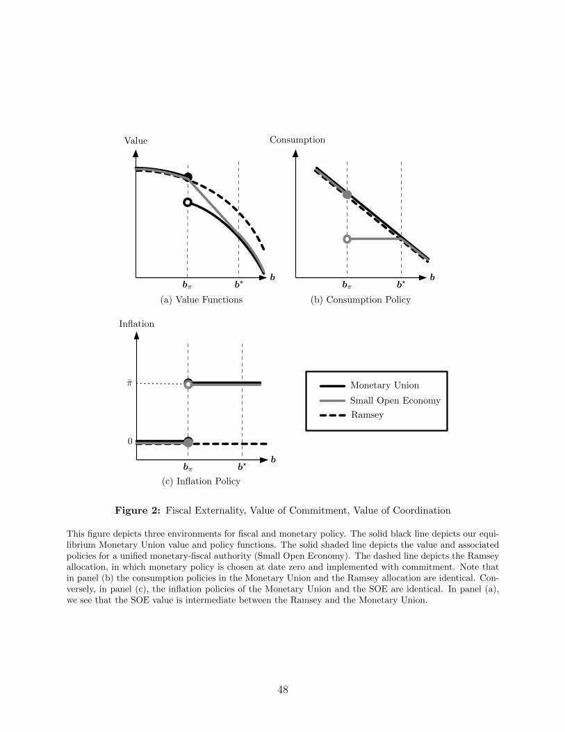
bb

(a) Value Functions (b) Consumption Policy

(c) Inflation Policy

bbb? b?

bb b?

0

Inflation

ConsumptionValue

Monetary Union

Small Open Economy

Ramsey

Figure 2: Fiscal Externality, Value of Commitment, Value of Coordination

This figure depicts three environments for fiscal and monetary policy. The solid black line depicts our equi-librium Monetary Union value and policy functions. The solid shaded line depicts the value and associatedpolicies for a unified monetary-fiscal authority (Small Open Economy). The dashed line depicts the Ramseyallocation, in which monetary policy is chosen at date zero and implemented with commitment. Note thatin panel (b) the consumption policies in the Monetary Union and the Ramsey allocation are identical. Con-versely, in panel (c), the inflation policies of the Monetary Union and the SOE are identical. In panel (a),we see that the SOE value is intermediate between the Ramsey and the Monetary Union.

48

R

b

0 1

A

B

C

D

Figure 3: Crisis threshold and debt composition

This figure depicts the equilibrium crisis threshold bλ as a function of the parameter η, which defines thefraction of debtors in the monetary union. The bold line is the equilibrium threshold at each η. The shadedline labelled R is defined in the text.

49

bbA

bB = bB

b?B

V B(b, b)

(a) Value (b) Value Net of Inflation (c) Inflation Costs

bbA

bB = bB

b?B

V A(b)

V B(b)

b?A b?A

V A(b, b)

bB = bB

b?B

0

V A(b) V A(b, b)

V B(b) V B(b, b)

b

Figure 4: Welfare and debt composition

This figure depicts the value function (panel a), the value net of inflation (panel b), and the inflation costs(panel c) for two values of η. The value in panel (a) is the value in panel (b) minus the costs in panel (c).The black line corresponds to η = 0, which is the zero-inflation case. The shaded line depicts the case ofη > 0 from point B in Figure 3.

50