Coordination Cascades:Sequential Choice in the Presence of a Network Externality

B. Curtis Eaton∗

The University of Calgary

and

David Krause∗∗

Competition Bureau Canada

September 2005

Abstract

In the network externality literature, little, if any attention has been paid to theprocess through which consumers coordinate their adoption decisions. The primaryobjective of this paper is to discover how effectively rational individuals manage tocoordinate their choices in a sequential choice framework. Since individuals maketheir choices with minimal information in this setting, perfect coordination will rarelybe achieved, and it is therefore of some interest to discern both the extent to whichcoordination may be achieved, and the expected cost of the failure to achieve perfectcoordination. We discover that when it counts, that is when the network external-ity is large, a substantial amount of coordination is achieved, and although perfectcoordination is never guaranteed, expected relative efficiency is large.

Keywords: Coordination Cascades, Network Externalities, Social Networks, Sequen-tial Choice

JEL Classification: L13

We would like to thank Zhiqi Chen, Jeffrey Church, Tom Cottrell, Alan Gunderson, KenMcKenzie, Krishna Pendakur, Michael Raith, Clyde Reed, and Guofu Tan for their in-sightful comments and encouragement. The views and opinions expressed in this articleare solely those of the authors and should not be interpreted as reflecting the views of theCommissioner of Competition, or other members of the staff.

* Corresponding author. Department of Economics, The University of Calgary, Calgary,Alberta, Canada, T2N 1N4. email : eaton@ucalgary.ca. ** Competition Policy Branch,Competition Bureau Canada, 50 Victoria Street, Gatineau, Quebec, Canada, K1A 0C9.email : krause.david@cb-bc.gc.ca.

1 Introduction

There is a large literature on network externalities.1 In this literature, the existence

of a network externality implies that the realized network benefit that an individ-

ual receives is dependent upon the number of other individuals who make the same

choice. As a result, when making her adoption decision an individual must form ex-

pectations concerning the number of individuals who will eventually choose the same

good. Despite the large literature on network externalities, relatively little work has

focused on the expectations formation problem that is at the core of the individual’s

choice problem in the presence of a network externality. Typically, the problem is ad-

dressed with a simplifying assumption, or it is ignored altogether. For example, Katz

and Shapiro (1985) resolve the problem by adopting the assumption that consumer

expectations are fulfilled in equilibrium. Of course, models with network externalities

have multiple equilibria, which raises yet another expectations formation question,

even if it is supposed that expectations are fulfilled in equilibrium: how is it that

consumers manage to coordinate their expectations on one of the possible equilibria?

That is, network externalities raise an equilibrium selection problem. To achieve any

of the equilibria, the expectations of all individuals must somehow be coordinated.

But if choices are made independently, there is nothing to assure that coordination

will in fact, be achieved. These problems are well known, and various authors have

suggested a variety of approaches to them (see for example, Farrell and Katz (1998)),

yet they remain unresolved. This is surprising given how important expectations are

when dealing with network externalities. As Farrell and Klemperer (2004) point out,

“how adopters form expectations and coordinate their choices dramatically affects

the performance of competition among networks.”

Notice also that when the process by which expectations are formed is swept

1See http://www.stern.nyu.edu/networks/site.html. See especially, Rohlfs (1974), Katz andShapiro (1985), Farrell and Saloner (1985), Church and Gandal (1992), Katz and Shapiro (1994),and Economides (1996).

1

away, so too is the ability to address a variety of interesting questions. Is it easier

to achieve coordination as the total number of consumers increases? If the value of

the network benefit is small, is coordination more difficult to achieve? Is it easier

to coordinate in an environment where tastes are similar? Are the expected costs of

the failure to achieve perfect coordination large? More generally, what facilitates and

what inhibits coordination? Our purpose in this paper is to explore these issues in a

sequential choice framework.

We approach the coordination problem in a framework that is suggested by the

literature on information cascades.2 In our model, choices are made sequentially, and

in making their choices individuals know their own preferences, the choices of people

who precede them in the choice making sequence, and very little else. Clearly, in

this setting perfect coordination will rarely be achieved, and it is therefore of some

interest to discern both the extent to which coordination may be achieved, and more

particularly, the expected cost of the failure to achieve perfect coordination, since

this magnitude would seem to have a direct bearing on the question of whether or

not unfettered markets can effectively solve the coordination problem associated with

a network externality. To preview results, it turns out that if the network exter-

nality in our model is sufficiently strong, individuals manage to achieve substantial

coordination.

The particular model that we use is a special case of the model of Katz and

Shapiro (1985).3 There are two goods, and two types of people. One type has a

private preference for one of the goods and the other has a private preference for

the other good. However, there is a network externality that potentially overwhelms

these private preferences. We restrict attention to parameter values such that there

2For a further discussion on information cascades see Bikhchandi et al (1992, 1998).3While the discussion in this paper focuses on issues that arise in the context of industrial

organization, the analysis is equally applicable to the literature on network externalities in thecontext of social interaction. See Leibenstein (1950), Akerlof (1980,1997), Becker (1991), Banerjee(1992), Glaeser and Scheinkman (2000), Eaton,Pendakur and Reed (2001) and Durlauf and Young(2001).

2

are two equilibria of the simultaneous choice game, in both equilibria all individuals

choose the same good, and both equilibria are Pareto-optimal. We examine both

the simultaneous move game, and the game that arises when decisions are made

sequentially, and compare the equilibrium of the sequential choice game with the

equilibrium of the corresponding simultaneous choice game.

Choi (1997) explores a technology adoption problem with network externalities in

a sequential choice setting. There are two technologies, A and B, and initially the

effectiveness of both is unknown. But once the first adopter has chosen a technology,

say technology A, its effectiveness is revealed to all. The second adopter then faces the

problem of whether to choose the untried technology B, or to follow the first adopter’s

lead and choose technology A. Because there are network effects, the second adopter

must ask herself what those who follow her will do. If she chooses B, and it turns out to

be more effective than A, those who follow will also choose B and the second adopter

will have a large network and the more effective technology. But if she chooses B and

it turns out to be less effective than A, those who follow will adopt A, and the second

mover will be stranded with no network. Hence, if the value of a network is large, the

expected effectiveness of technology B must be significantly greater than the known

effectiveness of technology A to induce the second adopter to choose technology B. In

that choices are sequential, this model is similar to ours. However, the nature of the

information problem is quite different. In our model, individuals use the choices of

those who precede them in the choice sequence to infer something about the relative

proportions of types of individual in the population, while in Choi’s model the choices

of predecessors resolve uncertainty about the technologies. As will become clear,

although the models are similar in one respect, the analytical approaches are quite

different, as are the results.

3

2 The Model

In our model there are two goods, good 1 and good 2, there are two types of individual,

type A and type B, there are many individuals of each type, and individuals choose

either good 1 or good 2. Goods have a purely private value that is type dependent,

and a network or social value that is driven by a numbers externality.

There are NA individuals of type A, NB of type B, and the total number of

individuals is N ≡ NA + NB. For a person of type i, the private value of good j

is zij. We assume that zA1 > zA2 and that zB2 > zB1, so that type A individuals

have a private preference for good 1, and type B a private preference for good 2. For

simplicity we assume that zA1 > 0 and zB2 > 0. For type A individuals the magnitude

of the private preference differential is DA ≡ zA1 − zA2, and for type B individuals

it is DB ≡ zB2 − zB1. In most of what we do in this paper, these differentials are

identical.

Network externalities are captured by a parameter S > 0 that we call potential

network value. If some person chooses good j, the realized network value for that

person is S · πj, where πj is the proportion of other people who also choose good

j. In other words, the potential network value is realized by an individual only

to the extent that the individual’s consumption decision is coordinated with the

consumption decisions of others.

Individuals choose either good 1 or good 2, but not both. Although some interest-

ing pricing issues arise in this model, we do not address them. Hence there is no need

to explicitly introduce prices. Instead, interpret zij as the private value to individual

i of good j net of the price of the good.

If Di > S, then private consumption values drive the choice of an individual of

type i. Consider, for example, a type A individual: DA > S implies that zA1 > zA2+S

so that the individual always prefers good 1 to good 2. Note that when both DA > S

4

and DB > S, there is a unique equilibrium in which type A individuals choose good 1

and type B individuals choose good 2, and that this equilibrium is Pareto-optimal. In

this case, the network externality raises no interesting issues. Accordingly, we assume

that DA < S and DB < S.

If we now imagine that choices are made simultaneously, there are two corner

equilibria in which everyone chooses either good 1 or good 2. To see this, consider

an individual of type A faced with a situation in which she anticipates that everyone

else will choose good 2. Since DA < S, it is the case that S + zA2 > zA1, and

the network effect leads the type A individual to choose good 2 in preference to her

privately preferred good, good 1. Since type B individuals clearly prefer good 2 when

they anticipate that everyone else will choose good 2, we have a corner equilibrium

in which everyone chooses good 2.

Notice that both corner equilibria are Pareto-optimal. Consider, for example, the

corner equilibrium in which everyone chooses good 2. In this equilibrium individuals

of type B are better off than they would be in any other situation, since they consume

the good that they privately prefer and they realize the full potential network value,

S. Hence, no other situation can Pareto-dominate this corner equilibrium. The

corner equilibrium in which everyone chooses good 1 will be cost benefit optimal if

NADA ≥ NBDB, and the other corner equilibrium will be cost-benefit optimal if

NBDB ≥ NADA.

We have then the familiar equilibrium selection problem associated with network

externalities. There are two equilibria, both of which are Pareto-optimal, but to

achieve either requires that the choices of all individuals be somehow coordinated. In

the simultaneous move game there is no obvious means of coordination, and hence

no assurance that either equilibrium will be achieved.

In this paper we assess the possibilities for coordination in a framework in which

individuals choose good 1 or good 2 in sequence, knowing only their own type, the

5

choices made by those who precede them in the choice making sequence, the taste

parameters of the model, and the total number of individuals in the choice making

sequence.

3 The Sophisticated Individual’s Choice Problem

Consider the decision problem of individual k in the choice making sequence. By

hypothesis, she knows the number of people who previously chose good 1, M1, and

the number who previously chose good 2, M2 (where M1 +M2 = k − 1); she knowsher own type, A or B; she knows the total number of people in the choice making

sequence, N ; and she knows the five taste parameters of the model, S, zA1, zA2, zB1,

and zB2. Although we distinguish five taste parameters, there are in fact just three

relevant taste parameters, S, DA, and DB.

Since her realized network value is dependent upon the number of other individuals

who make the same choice that she makes, she must form subjective probabilities

concerning the total number of people who will eventually choose good 1. (Since

everyone chooses one good or the other, we can focus on expectations with respect to

the number of people who eventually choose good 1.) Of course, the choices of those

who follow her in the sequence may depend upon her own choice, so she needs two

sets of subjective probabilities, which correspond to the two goods she might choose.

Define Gk(Q1;M1, i) as person k’s subjective probability that a total of Q1 individuals

other than k eventually choose good 1, given thatM1 of the first k−1 individuals havechosen good 1, and given that individual k chooses good i. With N − k individuals

following individual k in the choice making sequence, M1 ≤ Q1 ≤M1 +N − k.

Let zk1 and zk2 denote the private consumption values of individual k, where

(zk1, zk2) is either (zA1, zA2) or (zB1, zB2). Individual k will choose good 1 if the

6

following inequality is satisfied:

zk1 +S

N − 1 ·M1+N−kXQ1=M1

Q1 ·Gk(Q1;M1, 1) >

zk2 +S

N − 1 ·M1+N−kXQ1=M1

Q2 ·Gk(Q1;M1, 2), (1)

where Q2 = N − 1−Q1, and will choose good 2 if the inequality is reversed.

To solve this choice problem we must develop a calculus of subjective probability;

that is, we must develop the function Gk(Q1;M1, i), and then use it to solve person

k’s choice problem. Since these subjective probability distributions are, in effect,

a theory about the choices of the individuals who follow individual k in the choice

making sequence, the natural way to proceed is use a dynamic programming approach,

beginning with the choice problem of the last individual in the choice sequence, and

working our way back to individual k.

Before doing so, it is useful to define what we mean by a coordination cascade.

If M1, is large relative to k − 1 −M1, and if S is large enough, it will be the case

that individual k will choose good 1 regardless of her type, and that all individuals

who follow her in the choice making sequence will also choose good 1, regardless of

their type, and we say that individual k is trapped in a good 1 coordination cascade.

Alternatively, ifM1 is small relative to k−1−M1, and if S is large enough, individual k

is trapped in a good 2 coordination cascade. Individuals not trapped in a coordination

cascade will simply follow their private preferences, type A individuals will choose

good 1 and type B will choose good 2. If a coordination cascade arises early in the

choice sequence, then despite the lack of a coordinator, most individuals will choose

one good or the other, and we will end up at an equilibrium of the sequential choice

game that is close to one of the equilibria of the simultaneous choice game.

Once we have an understanding of coordination cascades, it is clear that to solve

7

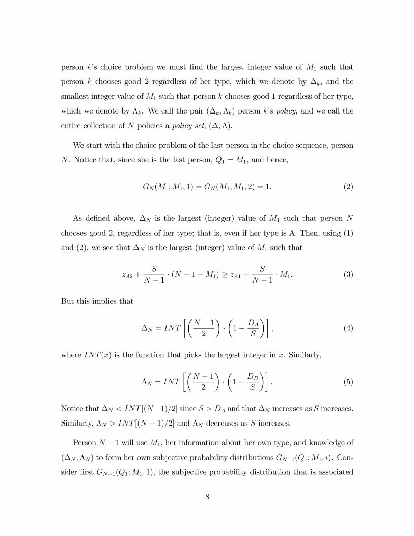
person k’s choice problem we must find the largest integer value of M1 such that

person k chooses good 2 regardless of her type, which we denote by ∆k, and the

smallest integer value ofM1 such that person k chooses good 1 regardless of her type,

which we denote by Λk. We call the pair (∆k,Λk) person k’s policy, and we call the

entire collection of N policies a policy set, (∆,Λ).

We start with the choice problem of the last person in the choice sequence, person

N . Notice that, since she is the last person, Q1 =M1, and hence,

GN(M1;M1, 1) = GN(M1;M1, 2) = 1. (2)

As defined above, ∆N is the largest (integer) value of M1 such that person N

chooses good 2, regardless of her type; that is, even if her type is A. Then, using (1)

and (2), we see that ∆N is the largest (integer) value of M1 such that

zA2 +S

N − 1 · (N − 1−M1) ≥ zA1 +S

N − 1 ·M1. (3)

But this implies that

∆N = INT

·µN − 12

¶·µ1− DA

S

¶¸, (4)

where INT (x) is the function that picks the largest integer in x. Similarly,

ΛN = INT

·µN − 12

¶·µ1 +

DB

S

¶¸. (5)

Notice that∆N < INT [(N−1)/2] since S > DA and that∆N increases as S increases.

Similarly, ΛN > INT [(N − 1)/2] and ΛN decreases as S increases.

Person N − 1 will use M1, her information about her own type, and knowledge of

(∆N ,ΛN) to form her own subjective probability distributions GN−1(Q1;M1, i). Con-

sider first GN−1(Q1;M1, 1), the subjective probability distribution that is associated

8

with the event that person N − 1 chooses good 1. As explained below

1. if M1 + 1 ≤ ∆N , then GN−1(M1;M1, 1) = 1;

2. if M1 + 1 ≥ ΛN , then GN−1(M1 + 1;M1, 1) = 1;

3. if ∆N < M1 + 1 < ΛN ,

then GN−1(M1 + 1;M1, 1) =M1+1N−1 ,

and GN−1(M1;M1, 1) =N−M1−2

N−1 .

If M1 + 1 ≤ ∆N and person N − 1 chooses good 1, then person N will be in a good

2 coordination cascade, and Q1 = M1 with probability 1. Similarly, if M1 + 1 ≥ ΛN

and person N − 1 chooses good 1, person N will be in a good 1 coordination cascade

and Q1 = M1 + 1 with probability 1. If ∆N < M1 + 1 < ΛN , then person N will be

in neither sort of cascade if person N − 1 chooses good 1, and hence person N ’s typewill determine her choice. If person N − 1 is type A, the information available to her(that she, andM1 of the first N − 2 persons in the choice sequence are type A) yieldsa subjective probability that person N is type A equal to (M1 + 1)/(N − 1) and asubjective probability that person N is type B equal to (N −M1 − 2)/(N − 1), asreported in 3 above. Of course, if person N −1 was type B her subjective probability

that person N is type A would be M1/(N − 1), but this subjective probability isirrelevant since person N − 1 will choose good 1 only if she is type A, since she is inneither sort of cascade.

We can find GN−1(Q1;M1, 2) in just the same way.

1. if M1 ≤ ∆N , then GN−1(M1;M1, 2) = 1;

2. if M1 ≥ ΛN , then GN−1(M1 + 1;M1, 2) = 1;

3. if ∆N < M1 < ΛN ,

9

then GN−1(M1 + 1;M1, 2) =M1

N−1 ,

and GN−1(M1;M1, 2) =N−1−M1

N−1 .

These subjective probability distributions in turn allow us to find the policy of

person N − 1, (∆N−1,ΛN−1). By definition, ∆N−1 is the largest integer M1 such that

zA2 +S

N − 1 ·M1+1XQ1=M1

Q1 ·GN−1(Q1;M1, 2) >

zA1 +S

N − 1 ·M1+1XQ1=M1

Q2 ·GN−1(Q1;M1, 1). (6)

Similarly, ΛN−1 is the largest integer M1 such that

zB1 +S

N − 1 ·M1+1XQ1=M1

Q1 ·GN−1(Q1;M1, 1) >

zB2 +S

N − 1 ·M1+1XQ1=M1

Q2 ·GN−1(Q1;M1, 2). (7)

We have then all that is needed to compute person (N − 1)’s policy, (∆N−1,ΛN−1).

Person N − 2 can use M1 (the number of persons who previously chose good 1),

her information about her own type, and knowledge of (∆N ,ΛN) and (∆N−1,ΛN−1)

to form her own subjective probability distributions GN−2(Q1;M1, i). This in turn

will allow person N − 2 to solve her own choice problem. This solution, of course, isdescribed by her policy, (∆N−2,ΛN−2). Then, building on these results, we can find

the policy of person N − 3, and so on.

It is tedious to actually compute these policies, and it becomes increasingly tedious

to do so as we move further up the choice making sequence. For this reason, we

have relied on numerical techniques to generate the policy set (∆,Λ) for particular

configurations of the model’s parameters, S, N , DA, and DB.

10

In Figure 1 we picture the policy set for the case in which N = 30, and S =

2.5 ·DA = 2.5 ·DB, so the potential network value is two and a half times as large as

the private preference differentials. The choice making sequence proceeds from top

to bottom in the figure. For each person k, the horizontal distance from one side of

the triangle to the other is equal to k−1, and it therefore serves as an axis forM1 for

that person. The jagged line on the left connects the ∆ks and the one on the right the

Λks. If person k finds herself in a situation where M1 is on or to the left of the first

jagged line, she and all who follow her are in a good 2 cascade, and if she finds herself

in a situation where M1 is on or to the right of the second jagged line, she and all

who follow her are in a good 1 cascade. And if she finds herself in a situation where

M1 lies between the jagged lines, she chooses the good that she privately prefers.

The policy set itself is reported at the bottom of Figure 1. Persons 1, 2 and 3 in

the choice sequence will all follow their private preferences. Person 4 will be trapped

in a good 2 cascade if none or just one of the first three people choose good 1, and she

will be trapped in good 1 cascade if two or three of the first three people choose good

1. This, of course, means that person 4 will definitely be trapped in one cascade or

the other. Since everyone who follows her will also be in cascade, just four terminal

states are possible. We can describe a terminal state by the number of persons in

total who choose good 1, T1, where T1 is an integer in the set {0, 1, ..., N}. If the firstthree people choose good 1, that is, if the first three people are all type A, then the

fourth is trapped in a good 1 cascade and T1 = 30. Analogously, if the first three all

choose good 2, T1 = 0. If two of the first three people choose good 1 (respectively

good 2), then the fourth is again trapped in a good 1 cascade (respectively good 2),

and T1 = 29 (respectively, T1 = 1). In this case, coordination is important since

S = 2.5 · DA = 2.5 · DB, and because it is so important, the fourth person in the

choice sequence is inevitably trapped in a cascade. The type of cascade that emerges

and the terminal state that is achieved depend on the types of the first three persons

in the choice sequence.

11

Good 2Cascade

Good 1Cascade

5 2920 251510

∆ Λ

N1

4

7

10

13

16

19

22

25

28

30

∆={∅,∅,∅,1,1,2,2,3,3,3,4,4,4,5,5,5,6,6,6,6,6,7,7,7,7,8,8,8,8,8}Λ={∅,∅,∅,2,3,3,4,4,5,6,6,7,8,8,9,10,10,11,12,13,14,14,15,16,17,17,18,19,20,21}

0

Figure 1: Policy Set for S = 2.5 ·DA = 2.5 ·DB

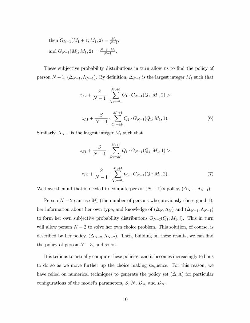
In Figure 2 we picture the policy set for the case in which N = 30, and S =

1.5 · DA = 1.5 · DB. Notice that the first opportunity for a cascade does not arise

until the sixth person makes her choice, and she will be trapped in a cascade if and

only if at least four of the first five people make the same choice. If a cascade does

not arise when the sixth person makes her choice, the next opportunity will not arise

until the tenth person makes her choice, and she will be in a cascade if and only if at

least seven of the first nine people are of the same type. With these parameter values

coordination is less important, and is very difficult to achieve.

12

Good 2Cascade

Good 1Cascade

5 2920 251510

∆ Λ

N1

4

7

10

13

16

19

22

25

28

30

∆={∅,∅,∅,∅,∅,∅,1,1,1,1,2,2,2,2,2,3,3,3,3,3,3,3,4,4,4,4,4,4,4,4}Λ={∅,∅,∅,∅,∅,∅,5,6,7,8,8,9,10,11,12,12,13,14,15,16,17,18,18,19,20,1,22,23,24,25}

0

Figure 2: Policy Set for S = 1.5 ·DA = 1.5 ·DB

4 The Naïve Individual’s Choice Problem

We have shown that if the network externality is sufficiently strong, individuals who

are sophisticated enough to perform the calculations envisioned in our model of se-

quential choice manage to achieve substantial coordination. As a point of comparison,

it is useful to compare these results with the corresponding results for naïve individ-

uals. Naïve individuals, by definition, do not take into account the effects that their

adoption decisions maight have on the adoption decisions of people who follow them

in the choice making sequence. Instead, they behave as if they were the last person

in the sequence.

Since naive individuals do not anticipate cascades, they do not form subjective

probabilities concerning the total number of people who will eventually choose good

13

1. However, coordination cascades can still arise, and therefore we must still calculate

the naive individuals’s policy. In solving person k’s choice problem we find the largest

integer value of M1 such that person k chooses good 2 regardless of her type, which

we now denote δk, and the smallest integer value of M1 such that person k chooses

good 1 regardless of her type, which we now denote λk. We call the pair (δk,λk) naïve

person k’s policy and we call the entire collection of N policies, (δ, λ), a naïve policy

set.

Since naïve individuals behave as if they aer the last person in the sequence, naïve

individual K will choose good 2 even if she is type A if the following inequality holds:

zA2 +S

K − 1 · (K − 1−M1) ≥ zA1 +S

K − 1 ·M1. (8)

This implies that

δK = INT

·µK − 12

¶·µ1− DA

S

¶¸(9)

and similarly,

λK = INT

·µK − 12

¶·µ1 +

DB

S

¶¸. (10)

In Figure 3 we picture the naïve policy set for the case in which N = 30, and

S = 2.5 ·DA = 2.5 ·DB. It is now the case that persons 1, 2, 3 and 4 in the choice

sequence will all follow their private preferences. Person 5 will be trapped in a good

2 cascade if none or just one of the first four people choose good 1, and she will be

trapped in a good 1 cascade if three or four of the first four people choose good 1.

However, if only two of the first four people choose good 1, then person 5 follows their

private preferences. In this case, it is no longer guaranteed that a cascade will form,

unlike the situation where individuals take into account the future effect of their

adoption decisions. In fact, for naïve individuals the probability of a coordination

cascade forming is always smaller than for sophisticated consumers.

14

Good 2Cascade

Good 1Cascade

5 2920 251510

δ λ

N1

4

7

10

13

16

19

22

25

28

30

δ={∅,∅,∅,∅,1,1,1,2,2,2,3,3,3,3,4,4,4,5,5,5,6,6,6,6,7,7,7,8,8,8}λ={∅,∅,∅,∅,3,4,5,5,6,7,7,8,9,10,10,11,12,12,13,14,14,15,16,17,18,19,19,20,21}

0

Figure 3: Naive Policy Set for S = 2.5 ·DA = 2.5 ·DB

5 Aggregate Results

In this section we examine aggregate choices for groups of individuals when the se-

quence in which the individuals make their choices is random. We report the proba-

bility distributions over terminal states and a measure of relative efficiency.

We use the following approach:

1. create a group of individuals by choosing values for the following parameters —

S, NA, NB, DA, and DB;

2. find the policy set for the given parameter values — the policy set depends on

the total number of people, N = NA +NB, but not on the numbers of people

of types A and B, and the preference parameters;

15

3. generate a frequency distribution over terminal states by choosing a large num-

ber (10,000 is the number used in the simulations reported below) of random

choice sequences for the group, and for each random sequence use the policy

set to determine the associated terminal state — the frequency distribution, in

turn, generates an approximate probability distribution over terminal states.

We calculate relative efficiency as follows. Let U∗ denote total utility in the cost-

benefit optimal equilibrium of the simultaneous choice game, Up denote total utility

when individuals follow their private preferences, UT denote total utility in terminal

state T , and pT the approximate probability of terminal state T . Relative efficiency

(RE), is then defined as follows:

RE =

¡PT p

TUT¢− UP

U∗ − UP. (11)

Notice that 0 ≤ RE ≤ 1. The denominator in this expression is the maximumpossible gain in utility, relative to the situation where people simply follow their

private preferences, and the numerator os the expected gain in utility relative to

the same point of comparison. Thus, RE measures the expected proportion of the

maximal gain in utility from achieving perfect coordination that is achieved in our

sequential choice model.

Results for the case in which S = 2.5, NA = 15, NB = 15, DA = 1, andDB = 1 are

reported in Figure 4. Recall that the policy set for this case is pictured in Figure 1.

For purposes of comparison, in the bottom half of the figure we report the frequency

distribution over terminal states, g(M), that would arise if individuals simply chose

the good that they privately prefer. Since there are 30 people in the group and

half of them are type A, the terminal state that is generated when people follow

their private preferences is T1 = 15. In the top half of the figure we report the

frequency distribution that is generated when individuals use the policy set to make

16

their choices. As we saw earlier, with this policy set the fourth person inevitably finds

herself in a coordination cascade, and there are just four possible terminal states:

T1 = 0, T1 = 1, T1 = 29, and T1 = 30. In our simulations, the relative frequency

of these terminal states is 0.115, 0.386, 0.388, and 0.110.4 The relative efficiency for

this case is 0.87, so the failure to achieve perfect coordination in this case results

in an expected aggregate increase in welfare, relative to the welfare achieved when

individuals follow their private preference, that is 87% of the maximal increase.

zA1=1zA2=0 zB1=0zB2=1

NA=15 NB=15

Figure 4: Results for S = 2.5 ·DA = 2.5 ·DB

To get a feeling for the comparative statics of this model with respect to S, in

4For this case we can easily calculate the actual probabilities of these terminal states, which servesas a very rough check on the accuracy of our approximation. Terminal states T1 = 0 and T1 = 30require that the first three individuals in the choice sequence be of the same type, an event thatwill occur with probability (15/30) · (14/29) · (13/28) which is approximately 0.112. Terminal statesT1 = 1 and T1 = 29 require that exactly two of the first three persons in the choice sequence be ofthe same type, which will occur with probability 3 ·(15/30) ·(14/29) ·(15/28), which is approximately0.388.

17

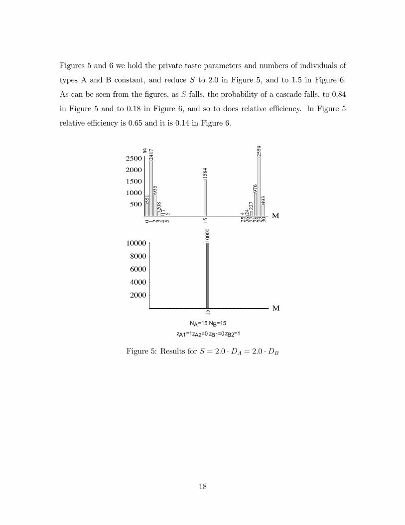
Figures 5 and 6 we hold the private taste parameters and numbers of individuals of

types A and B constant, and reduce S to 2.0 in Figure 5, and to 1.5 in Figure 6.

As can be seen from the figures, as S falls, the probability of a cascade falls, to 0.84

in Figure 5 and to 0.18 in Figure 6, and so to does relative efficiency. In Figure 5

relative efficiency is 0.65 and it is 0.14 in Figure 6.

NA=15 NB=15

zA1=1zA2=0 zB1=0zB2=1

Figure 5: Results for S = 2.0 ·DA = 2.0 ·DB

18

NA=15 NB=15

zA1=1zA2=0 zB1=0zB2=1

Figure 6: Results for S = 1.5 ·DA = 1.5 ·DB

In tables 1 and 2 we present further results concerning the degree to which co-

ordination is achieved, and expected relative efficiency as S varies, holding private

preference parameters and the numbers of individuals of each type constant at the

values specified above. Table 1 shows that coordination cascades begin to appear

when S is approximately 1.3. The probability of a cascade then increases quickly as

S increases. For S greater than approximately 2.1, the probability of a cascade is 1.5

The message is clear and intuitive: as coordination becomes more important, that is,

as S increases, it is more readily achieved.

The reason for the quick transition between no cascade forming and a cascade

always forming, is because cascades arise early in the sequence of choices. Since

individuals take into account what the individuals who follow them might choose,

5Note that for naïve individuals, for the results presented, the probability of a cascade formingis less than 1.

19

individuals at the beginning of the sequence will be more willing to start a cascade

then they would if they did not take future actions into account. Recall the discussions

of Figures 1 and 2. Figure 2 shows the policy set for S = 1.5. In that case, the

opportunity of a cascade does not arise until person 6. In contrast, in Figure 1,

cascades are inevitable (since the forth person is always in one cascade or the other).

As the network value S increases, the distance between the policy pairs decreases

thereby increasing the chances for a cascade forming early in the sequence of choices.

Table 1:Probability of Cascade wrt S

S

1.0 1.1 1.2 1.3 1.4 1.5 1.6 1.7

Sophisticated 0 0 0 0.03 0.09 0.18 0.35 0.40

Naïve 0 0 0 0.01 0.04 0.17 0.17 0.34

S

1.8 1.9 2.0 2.1 2.2 2.3 2.4 2.5

Sophisticated 0.70 0.72 0.84 1.0 1.0 1.0 1.0 1.0

Naïve 0.36 0.36 0.65 0.64 0.65 0.65 0.71 0.72

Table 2 tells us what happens to relative efficiency as S increases. At S = 1,

cascades never occur as individuals always follow their private preferences, and hence

relative efficiency is zero. As S increases, relative efficiency increases in step with the

increase in the probability of a cascade forming.

20

Table 2:Relative Efficiency wrt S

S

1.0 1.1 1.2 1.3 1.4 1.5 1.6 1.7

Sophisticated 0 0 0 0.02 0.06 0.14 0.27 0.31

Naïve 0 0 0 0.01 0.03 0.13 0.13 0.27

S

1.8 1.9 2.0 2.1 2.2 2.3 2.4 2.5

Sophisticated 0.56 0.57 0.65 0.85 0.86 0.86 0.87 0.87

Naïve 0.29 0.29 0.53 0.53 0.54 0.54 0.58 0.59

The case illustrated in Figure 5 serves as a baseline for the comparative static

exercises reported below. In Figure 7 we increase the number of individuals of each

type to 50, thus increasing the size of the group from 30 to 100, while holding the

other parameters constant. The probability of a cascade increases from 0.84 to 0.98,

and relative efficiency increases from 0.65 to 0.89.

21

NA=50 NB=50

zA1=1zA2=0 zB1=0zB2=1

Figure 7: Results for N = 100 and S = 2.0

Tables 3 and 4 report comparative statics concerning the degree to which coordi-

nation is achieved, and expected relative efficiency as the total number of individuals

varies, holding the network value, private preference parameters, and the numbers

of each type of individuals constant. Table 3 indicates that the probability of a

cascade increases as the size of the population increases, and table 4 indicates that

relative efficiency also increases as the size of the population increases. The message

is clear: larger groups are better able to achieve coordination in our sequential choice

framework.

22

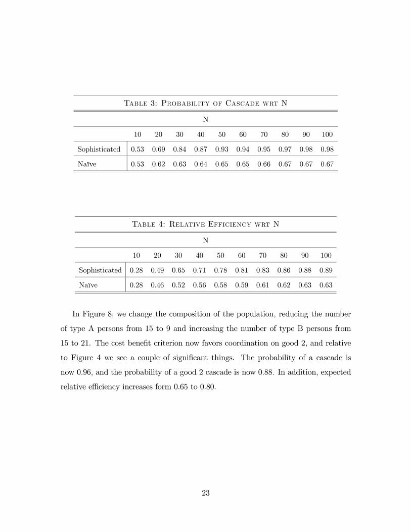
Table 3: Probability of Cascade wrt N

N

10 20 30 40 50 60 70 80 90 100

Sophisticated 0.53 0.69 0.84 0.87 0.93 0.94 0.95 0.97 0.98 0.98

Naïve 0.53 0.62 0.63 0.64 0.65 0.65 0.66 0.67 0.67 0.67

Table 4: Relative Efficiency wrt N

N

10 20 30 40 50 60 70 80 90 100

Sophisticated 0.28 0.49 0.65 0.71 0.78 0.81 0.83 0.86 0.88 0.89

Naïve 0.28 0.46 0.52 0.56 0.58 0.59 0.61 0.62 0.63 0.63

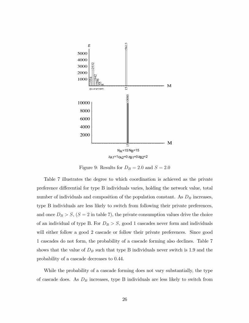
In Figure 8, we change the composition of the population, reducing the number

of type A persons from 15 to 9 and increasing the number of type B persons from

15 to 21. The cost benefit criterion now favors coordination on good 2, and relative

to Figure 4 we see a couple of significant things. The probability of a cascade is

now 0.96, and the probability of a good 2 cascade is now 0.88. In addition, expected

relative efficiency increases form 0.65 to 0.80.

23

NA=9 NB=21

zA1=1zA2=0 zB1=0zB2=1

Figure 8: Results for NA = 9, NB = 21, S = 2.0

Tables 5 and 6 illustrate the comparative statics in relation to the degree to which

coordination is achieved, and the expected relative efficiency as the composition of

the population varies, holding the network value, total number of individuals and

private preference parameters constant. Notice that coordination is easier to achieve

when the population consists of more like-minded individuals. For example, when

the number of type B individuals is 27 out of 30, the probability of a cascade is

essentially 1. As well, since coordination is easier to achieve in this case, expected

relative efficiency is also high, 0.88.6 Again, the message is clear: in our sequential

6The relative efficiency results for naïve individuals is due to the relationship between which typeof cascade forms and the number of each type of individual. When NA/N = 0.1, the probabilityof a good 2 cascade is less, and the probability of no cascade is higher, relative to the situationwith sophisticated individuals. In the naïve scenario, more individuals are choosing their privatelypreferred good, and thus, expected total utility is higher. However, the gain is not large because ofthe small number of type A individuals. When NA/N = 0.3, the gain is the largest. AtNA/N = 0.5,the relationship between the type of cascade and number of each type of individual balances out andrelative efficiency decreases (i.e. the number of individuals not consuming their privately preferred

24

choice framework, asymmetric populations achieve coordination more readily.

Table 5: Proability of Cascade wrt NA/N

NA/N

0.1 0.2 0.3 0.4 0.5

Sophisticated 0.99 0.99 0.96 0.89 0.84

Naïve 0.99 0.98 0.86 0.71 0.64

Table 6: Relative Efficiency wrt NA/N

NA/N

0.1 0.2 0.3 0.4 0.5

Sophisticated 0.88 0.81 0.80 0.75 0.65

Naïve 0.90 0.83 0.95 0.85 0.52

In Figure 9, we change the private preference differential for type B individuals,

DB, from 1 to 2.0. Since DA = 1 < DB = 2.0, type A individuals are less inclined

to follow their own preferences than are type B. This in turn implies that type A

individuals are more inclined to join a good 2 cascade than are type B individuals to

join a good 1 cascade. This is evident in Figure 9 which shows that relative to the

baseline case, the probability of a good 1 cascade has decreased from 0.42 to 0.

good increases).

25

NA=15NB=15

zA1=1zA2=0 zB1=0zB2=2

Figure 9: Results for DB = 2.0 and S = 2.0

Table 7 illustrates the degree to which coordination is achieved as the private

preference differential for type B individuals varies, holding the network value, total

number of individuals and composition of the population constant. As DB increases,

type B individuals are less likely to switch from following their private preferences,

and once DB > S, (S = 2 in table 7), the private consumption values drive the choice

of an individual of type B. For DB > S, good 1 cascades never form and individuals

will either follow a good 2 cascade or follow their private preferences. Since good

1 cascades do not form, the probability of a cascade forming also declines. Table 7

shows that the value of DB such that type B individuals never switch is 1.9 and the

probability of a cascade decreases to 0.44.

While the probability of a cascade forming does not vary substantially, the type

of cascade does. As DB increases, type B individuals are less likely to switch from

26

following their private preferences. This implies that the probability of a good 1

cascade should decrease as DB increases. Table 7 shows that as DB increases, the

probability of a good 1 cascade forming decreases from 0.45 at DB = 1 to 0.31 at

DB = 1.8, and then falls to 0 at DB = 1.9.7

Table 7: Probability of Cascade by Type of Cascade

DB

1.0 1.1 1.2 1.3 1.4 1.5 1.6 1.7 1.8 1.9 2.0

Sophisticated 0.84 0.84 0.84 0.84 0.84 0.84 0.82 0.81 0.72 0.44 0.44

Good 1 0.42 0.42 0.42 0.42 0.42 0.42 0.43 0.42 0.31 0 0

Good 2 0.42 0.42 0.42 0.42 0.42 0.42 0.39 0.39 0.41 0.44 0.44

Naïve 0.63 0.50 0.48 0.41 0.36 0.34 0.33 0.33 0.32 0.33 0.33

Good 1 0.31 0.18 0.17 0.09 0.04 0.02 0 0 0 0 0

Good 2 0.32 0.32 0.31 0.32 0.32 0.32 0.33 0.33 0.32 0.33 0.33

Finally, table 8 tells us what happens to relative efficiency as DB increases. Given

the amount of coordination that occurs, the measure of relative efficiency is small,

ranging from 0.34 when DB = 1.9 to 0.65 at DB = 1. The reason for the low

values of relative efficiency is due to the amount of coordination on good 1 that

still occurs. Good 1 has a lower average private preference value than good 2, and

therefore maximum utility is achieved when everyone coordinates on good 2.8 Since

good 1 cascades can still form, the realized gain in utility from coordination is not

maximized. Therefore, while there still exists a substantial amount of coordination,

7For naïve individuals the probability of a good 1 cascade forming declines quickly. The reasonis that naïve type B individuals do not forecast the future benefits of joining a good 1 cascade, andthe benefits of choosing good 1 when it is their turn to choose due not outwiegh their strong privatepreference for good 2.

8When private preference values are symmetric, maximum utility can be achieved through perfectcoordination on either good.

27

there is no guarantee that individuals will coordinate on the good that yields the

greater total utility.

Table 8: Relative Efficiency wrt DB

DB

1.0 1.1 1.2 1.3 1.4 1.5 1.6 1.7 1.8 1.9 2.0

Sophisticated 0.65 0.61 0.57 0.53 0.50 0.45 0.42 0.38 0.35 0.34 0.34

Naïve 0.52 0.39 0.37 0.31 0.29 0.27 0.27 0.27 0.26 0.27 0.27

6 Conclusion

In the network externality literature, perfect coordination of consumer choices on one

option is optimal, yet it is clear that in the absense of some sort of central direction,

it is highly unlikely that perfect coordination will, in fact, be achieved. The question

of interest would then seem to be: Given that consumer decisions are not centrally

directed, what are the costs of the failure to achieve perfect coordination? We address

this question in a sequential choice framework in which consumers observe the choices

of those who precede them and anticipate the choices of those who follow them.

The most interesting comparative static results relate to the magnitude of the

network externality and the size of the group. Both the probability of a coordina-

tion cascade, in which a large majority of consumers choose the same good, and the

expected relative efficiency of the sequential choice equilibrium, increase as the mag-

nitude of the network externality increases and as group size increases. In both cases,

the probability of a cascade rapidly approaches 1, and relative efficiency increases to

the 85% range. Thus, when it really counts, unfettered and undirected choice making

effectively solve the coordination and equilibrium selection problems that are raised

28

by the network externality in our model.

29

References

[1] Akerlof, G.A., 1997, “Social Distance and Social Decisions,” Econometrica,65:1005-1027.

[2] Akerlof, G.A., 1980, “A Theory of Social Custom, of Which Unemployment Maybe One Consequence,” The Quarterly Journal of Economics, 84:749-775.

[3] Ambrus, A., and R. Argenziano, 2004, “Network Markets and Consumer Coor-dination,” Cowles Foundation Discussion Paper No. 1481.

[4] Banerjee, A.V., 1992, “A Simple Model of Herd Behavior,” The Quarterly Jour-nal of Economics, 107:797-817.

[5] Becker, G., 1991, “A Note on Restaurant Pricing and Other Examples of SocialInfluence on Price,” Journal of Political Economy, 99:1109-1116.

[6] Bikhchandi, S., D. Hirshleifer, and I. Welch, 1992, “A Theory of Fads, Fashion,Custom and Cultural Change as Informational Cascades,” Journal of PoliticalEconomy, 100:992-1026.

[7] Bikhchandi, S., D. Hirshleifer, and I. Welch, 1998, “Learning from the Behaviourof Others: Conformity, Fads, and Informational Cascades,” Journal of EconomicPerspectives, 12:151-170.

[8] Cabral, L. M. B., 1990, “On the Adoption of Innovations with ‘Network’ Exter-nalities,” Mathematical Social Sciences, 19:299-308.

[9] Choi, J. P., 1994a, “Irreversible Choice of Uncertain Technologies with networkExternalities,” RAND Journal of Economics, 25:382-401.

[10] Choi, J. P., 1994b, “Network Externality, Compatibility Choice, and PlannedObsolescence,” Journal of Industrial Economics, 42:167-182.

[11] Choi, J. P., 1997, “Herd Behavior, the ‘Penguin Effect,’ and the Suppression ofInformational Diffusion: An Analysis of Informational Externalities and PayoffInterdependency”, RAND Journal of Economics, 28:407-425.

[12] Church, J. and N. Gandal, 1992, “Network Effects, Software Provision, andStandardization,” Journal of Industrial Economics, XL:85-104.

[13] Church, J. and N. Gandal, 1993, “Complementary Network Externalitiesand Technological Adoption,” International Journal of Industrial Organization,11:239-60.

[14] Church, J. and I. King, 1993, “Bilingualism and Network Externalities,” Cana-dian Journal of Economics, 26:337-45.

30

[15] Dasgupta, A., 2000, “Social Learning with Payoff Complementarities,” Mimeo,Yale University.

[16] De Vaney, A. and C. Lee, 2001, “Quality Signals in Information Cascades and theDynamics of the Distribution of Motion Picture Box Office Revenues,” Journalof Economic Dynamics and Control, 25:593-614.

[17] Durlauf, S.N. and H.P. Young, 2001, Social Dynamics, Cambridge: MIT Press.

[18] Eaton, B.C., K. Pendakur, and C. Reed, 2001, “Culture as a Shared Experience,”University of Calgary, Department of Economics, Discussion Paper 2001-27.

[19] Economides, N., 1996a, “The Economics of Networks,” International Journal ofIndustrial Organization, 14:673-701.

[20] Economides, N., 1996, “Network Externalities, Complementarities, and Invita-tions to Enter,” European Journal of Political Economy, 12:211-33.

[21] Economides, N. and C. Himmelberg, 1995, “The Critical Mass and Network Sizewith Application to the US FAXMarket,” Discussion Paper No. EC-95-11, SternSchool of Business, N.Y.U. mimeo.

[22] Farrell, J. and M. Katz, 1998, “The Effects of Antitrust and Intellectual PropertyLaw on Compatibility and Innovation,” The Antitrust Bulletin, XLIII:609-650.

[23] Farrell, J. and P. Klemperer, 2004, “Coordination and Lock-In: Competi-tion with Switching Costs and Network Effects,” Mimeo, Oxford University(http://www.paulklemperer.org).

[24] Farrell, J. and G. Saloner, 1985, “Standardization, Compatibility, and Innova-tion,” RAND Journal of Economics, 16:70-83.

[25] Farrell, J. and G. Saloner, 1986a, “Standardization and Variety,” EconomicsLetters, 20:71-74.

[26] Farrell, J. and G. Saloner, 1986b, “Installed Base and Compatibility: Innova-tion, Production Preannouncements and Predation,” American Economic Re-view, 76:940-55.

[27] Fudenberg, D. and J. Tirole, 2000, “Pricing a Network Good to Deter Entry,”Journal of Industrial Economics, 48:373-90.

[28] Glaeser, E.L. and J. Scheinkman, 2000, “Non-Market Interactions,” NBERWorking Paper No. W8053.

[29] Karni, E., and D. Schmeidler, 1990, “Fixed Preferences and Changing Tastes,”American Economic Review, 80:262-267.

31

[30] Karni, E., and D. Levin, 1994 “Social Attributes and Strategic Equilibrium: ARestaurant Pricing Game,” Journal of Political Economy, 102:822-840.

[31] Katz, M., and C. Shapiro, 1985, “Network Externalities, Competition and Com-patibility,” American Economic Review, 75:424-40.

[32] Katz, M. and C. Shapiro, 1986, “Technology Adoption in the Presence of NetworkExternalities,” Journal of Political Economy, 94:822-41.

[33] Katz, M. and C. Shapiro, 1992, “Product Introduction with Network Externali-ties,” Journal of Industrial Economics, 40:55-83.

[34] Katz, M. and C. Shapiro, 1994, “Systems Competition and Network Effects,”The Journal of Economic Perspectives, 8:93-115.

[35] Leibenstein, H., 1950, “Bandwagon, Snob and Veblen Effects in the Theory ofConsumers’ Demand,” The Quarterly Journal of Economics, 64:183-207.

[36] Liebowitz, S.J. and S.E. Margolis, 1994, “Network Externality: An UncommonTragedy,” The Journal of Economic Perspectives, 8:133-50.

[37] Mason, R., 2000, “Network Externalities and the Coase Conjecture,” EuropeanEconomic Review, 44:1982-92.

[38] Michihiro, K. and R. Rob, 1998, “Bandwagon effects and Long Run TechnologyChoice,” Games and Economic Behaviour, 22:30-60.

[39] Postrel, S. R., 1990, “Competing Networks and Proprietary Standards: The Caseof Quadraphonic Sound,” Journal of Industrial Economics, 39:169-85.

[40] Rohlfs, J., 1974, “A Theory of Interdependent Demand for CommunicationsService,” Bell Journal of Economics and Management Science, 5:16-37.

[41] Witt, U., 1997, “‘Lock-In’ vs. ‘Critical Masses’ — Industrial Change under Net-work Externalities,” International Journal of Industrial Organization, 15:753-73.

32