coping with the collapse: a stock-flow consistent · pdf filecoping with the collapse: a...
TRANSCRIPT

Coping with the Collapse: A Stock-Flow ConsistentMonetary Macrodynamics of Global Warming∗
Gael Giraud† Florent Mc Isaac‡ Emmanuel Bovari§Ekaterina Zatsepina¶
July 27, 2016
Abstract
This paper presents a macroeconomic model of endogenous growth that enablesus to take into consideration both the economic impact of climate change and thepivotal role of private debt. Using the Goodwin-Keen approach [25], based onthe Lotka-Volterra logic, we couple its nonlinear dynamics with abatement costs.Moreover, various damage functions a la Nordhaus ([38]) and Dietz-Stern ([6])reflect the loss in final production due to the temperature increase caused by therising levels of CO2 emissions. An empirical estimation of the model at the world-scale enables us to simulate plausible trajectories for the planetary business-as-usualscenario. Our main finding is that, even though the short-run impact of climatechange on static economic fundamentals may seem prima facie rather minor, itslong-run dynamic consequences may lead to an extreme downside. Under plausiblecircumstances, global warming forces the private sector to leverage in order tocompensate for output losses; the private debt overhang may eventually induce aglobal financial collapse, even before climate change could cause serious damage tothe production sector. Under more severe conditions, the interplay between globalwarming and debt may lead to a secular stagnation followed by a collapse in thesecond half of this century. We analyze the extent to which slower demographicgrowth or higher carbon pricing allow a global breakdown to be avoided. The paperconcludes by examining the conditions under which the +1.5◦C target, adopted bythe Paris Agreement (2015), could be reached.
Keywords Climate change, endogenous growth, damage function, integrated assess-ment, collapse, stock-flow consistency, Goodwin, debt, secular stagnation.
JEL Classification Numbers: C51, D72, E12, O13, Q51, Q54∗This work benefited from the support of the Energy and Prosperity Chair. We thank Antonin Pottier
and participants of the World Bank conference “The State of Economics. The State of the World” (June16, 2016) for helpful suggestions, as well as Ivar Ekeland, Herve Le Treut, and Nick Stern for theirencouragements. All errors are, of course, our own.†AFD - Agence Francaise de Developpement, Universite Paris 1 - Pantheon-Sorbonne; CES, Centre
d’Economie de la Sorbonne.‡AFD - Agence Francaise de Developpement, Universite Paris 1 - Pantheon-Sorbonne; CES, Centre
d’Economie de la Sorbonne.§AFD - Agence Francaise de Developpement¶Universite Paris 1 - Pantheon-Sorbonne; CES, Centre d’Economie de la Sorbonne. This author
gratefully acknowledges the financial support of ADEME.
1

Coping with the Collapse: A Stock-Flow Consistent Monetary Macrodynamics ofGlobal Warming
1 Introduction
Taking advantage of over forty years of hindsight available since The Limits to Growthwas published (Meadows et al(1972,1974)[34],[33], LtG in the sequel), several attempts toreview how society is tracking relative to their ground-breaking modeling have addressedthe question of whether the global economy is on a path of sustainability or collapse.Turner (2008, 2012, 2014)[53],[54],[55] and Hall and Day (2009)[23] (see also Jacksonand Webster (2016)[24]) tend to confirm the LtG standard-run scenarios, which forecasta collapse in living standards due to resource constraints in the twenty-first century.The mechanism underlying the simulated breakdown indeed seems consistent with theincreasing capital costs of peak oil and net energy (i.e., the decline of energy returned onenergy invested, EROI). On the other hand, over a similar time frame, international effortsbased around a series of United Nations (UN) conferences have yielded rather mixedresults (Linner and Selin, 2013[29], Meadowcroft, 2013[32]). In these simulations at least,the unraveling of the global economy and environment is essentially due to the growingscarcity of natural resources (energy, minerals, water...), while climate change plays littlerole, if any.1 Given the ongoing awareness of climate change damages, crystallized at thediplomatic level in the Paris Agreement of December 2015, this raises the question ofwhether global warming might per se induce a similar breakdown of the world economy.
This paper studies the conditions under which the answer to this question might bepositive, assuming that the world population will follow the UN median demographicscenario (see World Population Prospects 2015 – Data Booklet[1]). At variance with theliterature just mentioned, however, we explicitly model the financial side of the worldeconomy in order to assess the possible negative feedback of private debt on the ability ofthe world economy to cope with planetary damages. Besides these two basic modifications– our focus on climate warming rather than resource depletion, and on explicit intertwinedfinance–environment dependencies – the basic mechanism at work turns out to add a newdimension, absent from the narrative initially emphasized by LtG, namely the pivotal roleof private debt. Our own storyline goes as follows: losses due to environmental damagesforce the global productive sector to invest a growing part of its wealth in restoringand maintaining capital. As damages become more severe, current profits are no longersufficient to fund investment. Yet, investment keeps growing, courtesy of the lendingfacilities provided by the world banking sector. The lingering level of debt, however,may endanger the world’s economic engine itself as it is based on the promise of futurewealth creation: whenever the aggravation of climate damages prevents this promisefrom holding water, the productive sector may indeed become incapable of paying backits debt. Depending on the speed at which labor productivity increases compared to theseverity of global warming, the shrinking of investment induced by the burden of privatedebt may prevent the world economy from further adapting to climate turmoil, leadingultimately to a collapse around the end of the twenty-first century.
In the same way as LtG deliberately leaves the timeline somewhat vague, the maininterest of our findings lies, in our view, in the general pattern of behavior they highlight,rather than when exactly particular events might happen.
Finally, the global unraveling captured in this paper can be interpreted as the resultof a debt-deflation depression in the sense given to this concept by Irving Fisher (1933)[8].
1In LtG, of course, scenario 2 simulates a breakdown due to pollution, but the latter does not incor-porate the impact of global warming.
2

Coping with the Collapse: A Stock-Flow Consistent Monetary Macrodynamics ofGlobal Warming
The fact that part of the world economy might be on the verge of falling into a liquiditytrap is illustrated today by the two “lost decades” of Japan, of course, but also by therecessionary state of the southern part of the Eurozone, by obstinately negative long-terminterest rates on international financial markets and, last but not least, by the brutalcontraction of world nominal GDP in 2015 (-6%, IMF (2016)[9]). These paradoxes maybe viewed as signals that a secular decline induced by biophysical constraints is seepingthe financial sphere. To the best of our knowledge, this paper offers the first narrativewhere debt-deflation becomes the hallmark of a possible forthcoming breakdown provokedby global warming.
1.1 The dynamics of debtSince the financial crisis of 2007-2009, the ideas of Hyman Minsky around the intrinsic
instability of a monetary market economy have experienced a significant revival. In thesequel, we adopt a mathematical formalization of Minsky’s standpoint in order to assessthe role of debt dynamics in our narrative.2 More precisely, our starting point is the basicLotka-Volterra dynamics first introduced by Goodwin (1965)[15] and later extended byKeen (1995)[25]. Keen’s model (1995)[25] is a three-dimensional non-linear dynamicalsystem describing the time evolution of the wage share, employment rate, and privatedebt in a closed economy. Under reasonable assumptions, this system admits, amongothers, two locally stable long-run equilibria: one with a finite level of debt and nonzerowages and employment rate, and another characterized by infinite debt and vanishingwages and employment (Grasselli and Costa-Lima (2012)[18]). We show how the additionof a climate backloop, modeled through appropriately selected damage and abatementfunctions, drives the state of the economy towards long-run equilibrium with unlimiteddebt, leading to a planetary downside.
Over the past thirty years many integrated assessment models (IAMs in the sequel)have been developed in order to estimate the impact of economic development on theenvironment. A solid body of literature compares IAM models describing their advan-tages and disadvantages (Schwanitz (2013)[44]). The models considered in this literaturefall into one of four categories, based on the macroeconomic models they rely on: (1)welfare maximization; (2) general equilibrium; (3) partial equilibrium; and (4) cost min-imization (Stanton et al. (2009)[47]). By contrast, our modeling approach is based ona minimal (bounded) rationality requirement on the behavior of imperfectly competitivefirms, allows for multiple long-run equilibria, is stock-flow consistent (Godley and Lavoie(2012)[14]), and exhibits endogenous monetary cycles and growth, viscous prices, privatedebt, and underemployment. Moreover, money is endogenously created by the bankingsector (Giraud and Grasselli (2016)[11]) and turns out to be non-neutral (Giraud andKockerols (2016)[12]). The non-trivial properties of money enables the emergence of aphenomenon such as debt-deflation (Grasselli et al. (2015)[20]). Here, at variance withgeneral equilibrium approaches (see, e.g., Giraud and Pottier (2015)[13]), debt-deflationneed not just appear as a “black swan” – or, more precisely, a “rare” event relegatedto the tail of risk distribution. On the contrary, depending on the basin of attractionwhere the state of the economy is driven by climate damages, the ultimate breakdownmay occur as the inescapable consequence of the business-as-usual (BAU) trajectory.
2Dos Santos (2005)[43] provides a survey up to 2005 of the literature on the modeling of Minskianinstability; more recent contributions include Ryoo (2010)[42] and Chiarella and Guilmi (2011)[4].
3
Coping with the Collapse: A Stock-Flow Consistent Monetary Macrodynamics ofGlobal Warming
Approaches based on exogenous technology lead to three different types of answersto (some of) these questions depending on their assumptions. Somewhat oversimplify-ing existing approaches and assigning colorful labels, we can summarize these as follows.Nordhaus’ answer is that limited and gradual interventions are necessary (see Nordhaus(2007)[38]). Optimal regulation should reduce long-run growth by only a modest amount.Stern’s answer (see Stern (2013)[48]) is less optimistic. It calls for more extensive andimmediate interventions, and argues that these interventions need to be in place per-manently even though they may entail significant economic cost. The more pessimisticGreenpeace answer is that essentially all growth needs to come to an end in order to savethe planet.
The answer provided by the thought experiments run in this paper clearly standson the side of Stern’s viewpoint: as we shall show in companion papers, fundamentalbifurcations led by strong interventions may prevent the economic world from a disasterbut they are not detailed here. Rather, we focus on the business-as-usual perspective,and show that gradual and marginal interventions will not suffice: too narrow an answerto the climate challenge may lead to an end of growth by disaster (not by design) and toforced degrowth.
1.2 The climate and economy interactionBy contrast with the literature based on the Ramsey-Cass-Koopmans model, we incor-
porate endogenous drivers of growth and allow climate change to damage these drivers.As argued indeed by Stern (Stern (2006)[49]), climate change could have long-lastingimpacts on growth. We borrow from the emerging body of empirical evidence pointingin this direction (e.g., Dell et al. (2012)[5]), even though climatic conditions in the recentpast have been relatively stable compared with what we now have to contemplate in thenear future – which suggests that the “real story” might be even worse than what we areable to forecast.
Second, we consider various types of convexity of the damage function linking theincrease in global mean temperature with the instantaneous reduction in output. Thatit might be highly convex at some temperature is strongly suggested by the literature ontipping points (see Dietz-Stern (2015)[6] and Weitzman (2012)[58]). By contrast, mostexisting IAM studies assume very modest curvature of the damage function. The DICEdefault, for instance, is quadratic, and our simulations confirm that it leads to unrealisticnarratives (see Section 4.1 below).
Third, following Dietz-Stern (2015)[6] and Weitzman (2012)[58], we allow for ex-plicit and large climate risks by considering the possibility of high values of the climate-sensitivity parameter (i.e., the increase in global mean temperature, in equilibrium, ac-companying a doubling in the atmospheric concentration of CO2). We conduct sensitivityanalysis on high values, but also specify a probability distribution reflecting the latestscientific knowledge on the climate sensitivity as set out in the recent IPCC report (IPCC,2013[51]). Its key characteristic is a fat tail of very high temperature outcomes that areassigned low probabilities. By contrast, most IAM studies have ignored this key aspect ofclimate risk by proceeding with a single, best-guess value for the climate sensitivity, typ-ically corresponding to the mode of the IPCC distribution. Even though the IntentionalNationally Determined Contributions reported by the Parties to the Paris Agreement(see also IPCC, 2013[51]) should induce an average increase in temperature of 3.5◦C bythe end of this century, it is known that they are compatible with a 10% probability of
4

Coping with the Collapse: A Stock-Flow Consistent Monetary Macrodynamics ofGlobal Warming
reaching +6◦C. We show that the path leading to such a level of warming would lead to aplanetary collapse in the second half of this century. As written by Dietz-Stern (2015)[6]:“this is not just a ‘tail’ issue.”
The brief overview of collapses provided, e.g., in (Motesharrei et al.(2014)[35], p.91)not only shows the ubiquity of cycles of rise-and-collapse, but also the extent to whichadvanced, complex, and powerful societies are susceptible to collapse, even precipitously:“The fall of the Roman Empire, and the equally (if not more) advanced Han, Mauryan,and Gupta Empires, as well as so many advanced Mesopotamian Empires, are all tes-timony to the fact that advanced, sophisticated, complex, and creative civilizations canbe both fragile and impermanent.” In the thought experiment suggested in Motesharreiet al.(2014)[35], the authors argue that the Lotka-Volterra dynamics might be the secretdynamical invariant explaining this seemingly universal process of overshoot and collapse.Here, we partially confirm this suggestion by showing that the prey-predatory dynam-ics, when properly introduced into a macroeconomic framework through the interplaybetween debt, employment, and wages, leads to a similar conclusion: the world economy,as we know it today, is not immune to such a fate.
The paper is organized as follows: Section 2 sets the scene by introducing the stock-flow consistent macroeconomic model in presence of damage and abatement costs. InSection 3, the climate module is presented, describing the interconnection between theoutput level, emissions, CO2 concentration, average atmosphere temperature increase,and damages induced by climate change. Section 4 discusses the different scenariosarising from the interplay of our various key parameters. The final section summarizesthe conclusions and outlines areas for future research.
2 Monetary macrodynamicsOur underlying macroeconomic model closely follows the contribution of Grasselli and
Costa-Lima (2012)[18] and the literature centered around Keen’s (1995)[25] approach suchas Graselli et al. (2012, 2014, 2015)[18],[17],[20] and Nguyen-Huu et al. (2014)[36] amongothers. This framework, based on a Lotka-Volterra logic, is motivated by the aftermathof the 2008 sub-prime mortgage crisis, during which private debt played a pivotal role inendangering the world’s macroeconomic stability. One appeal of this literature lies in itsability to formalize economic collapse as a consequence of overindebtedness. We departfrom this literature, however, by endogenizing labor productivity growth, and add to theresulting structure climate-change feedback including temperature, abatement costs, anda damage function.
2.1 The basicsAbsent any damages due to climate change, the ”gross” real output, Y ∗, is linked to
the stock of productive capital, K, by a linear relationship, where, for simplicity, thecapital-to-output ratio, ν > 0, is assumed to be constant,
Y ∗ := K
ν.
5

Coping with the Collapse: A Stock-Flow Consistent Monetary Macrodynamics ofGlobal Warming
In this paper, ν ' 2.89.3 Introducing a damage function as in Nordhaus (2013)[40],current production is cut so that the global supply diminishes by the quantity DK
ν,
induced by global warming. Real output, Y , becomes
Y := (1−D)Kν. (1)
The damage function, D, is an increasing nonlinear function of the global atmospherictemperature deviance relative to its value, T , in 1900, defined shortly.
Let D denote the nominal private debt of firms. Its evolution depends upon the gapbetween nominal investment, pI, plus nominal dividends paid to the firms’ shareholders,Di, and current nominal profit, Π, that is,
D := pI +Di− Π, (2)
where p is the current price of consumption. The current nominal profit, Π, is
Π := pY −W − rD,
with W being the nominal wage bill, and r the (constant) short-term nominal interestrate.4 Denoting the total workforce by N , and the number of employed workers by L, theproductivity of labor, the employment rate, and the nominal wage per capita are givenrespectively by
a := Y ∗
L, λ := L
Nand, w = W
L. (3)
Denoting ω := wL/pY the wage share, and d := D/pY the private debt ratio, netprofit becomes Π = (1− ω − rd)pY . In the sequel, we denote by
π := 1− ω − rd (4)
the net profit share. Capital accumulation obeys the standard equation, expressed in realterms as
K := I − δK,
where δ is the constant depreciation rate of capital. Net investments are equal to grossinvestments minus abatement costs (defined shortly) paid by investors, that is,
I := Y (κ(π)− µG), (5)
where κ(·) is an increasing function of π, G ∈ [0, 1] denotes the real abatement costsimposed on the economy, and µ ∈ [0, 1] is measuring the fraction of abatement costs paidby investors. The function κ(·) will be empirically estimated.5
3See Appendix E.1 for details. The extension to an endogenous capital-to-output ratio is left forfurther research.
4Here, for simplicity, r is kept constant. We shall endogenize it and analyze in depth the impact ofTaylor rules in a subsequent paper.
5See Appendix E.4 for details. We refrain from trying to provide micro-foundations to either κ(·) orΦ(·). Indeed, as shown by Mas-Colell (1995)[31], full-blown rational corporates, when they are sufficientlynumerous, are exposed to an “everything-is-possible” theorem a la Sonnenschein-Mantel-Debreu at theaggregate level. Our phenomenological approach allows for this kind of emergence phenomena.
6

Coping with the Collapse: A Stock-Flow Consistent Monetary Macrodynamics ofGlobal Warming
Here, as in both the Goodwin and Keen models, the behavior of households is fully ac-commodated in the sense that, given the investment function, consumption is determinedby the accounting identity
C := Y − I = (1− κ(π)− µG)Y,
precluding more general specification of households saving propensity.6 Table 1 makesexplicit the stock-flow consistency of our model.
Households Firms Banks SumBalance SheetCapital stock pK pKLoan −D DSum (net worth) Xf Xb X
Transactions current capitalConsumption −pC pCInvestment pI −pIAccounting memo [GDP] [pY (1−D)]Wages W −WInterests on debt −rD rDFirms’ net profit −Π ΠDividends Di −Di
Financial Balances −D Πb
Flow of fundsGross Fixed Capital Formation pI pIChange in loans −D D
Column sum Π−Di D pI
Change in net worth Xf = Π−Di+ (p− δp)K Xb = Πb X
Table 1: Balance sheet, transactions, and flow of funds in the world economy.
It can be readily checked that, in this set-up, the accounting identity “investment =saving” always holds. This model departs from Grasselli et al. (2015)[20] in four ways.First, it includes damages induced by climate change. Second, we make explicit the divi-dends paid by firms to households. Third, as we shall see infra, labor productivity growthwill be endogenous. Fourth, the labor force is no longer assumed to grow exponentiallybut rather according to a sigmoid inferred from the 15–64 age group in the United Nationsscenario, World Population Prospects 2015 – Data Booklet.[1]
N
N:= q
(1− N
M
),
where M ≈ 7.056 billion is the upper bound of the labor force on Earth and q is the speedof convergence towards M (i.e., basically, the pace at which the demographic transitionis assumed to take place in sub-Saharan Africa).7
6Studying the consequences of dropping Say’s law will be the task of a forthcoming paper.7The estimation of the vector (q,M) is detailed in Appendix C.
7

Coping with the Collapse: A Stock-Flow Consistent Monetary Macrodynamics ofGlobal Warming
2.2 Endogenous monetary cyclesThe link between the real and nominal spheres of the economy is provided by a short-
run wage-price dynamics taken from Grasselli and Nguyen-Huu (2014)[21].8
w
w:= φ(λ) + γi, (6)
where 0 ≤ γ ≤ 1, ηp > 0, m ≥ 1, and
i = p
p:= −ηp
(1−m w
(1−D)pa
)+ c = ηp(mω − 1) + c. (7)
Equation (6) states that workers bargain for wages based on the current state of (un)employment(as in Keen (1995)[25]), but also take into account the observed inflation rate, i. Theconstant γ measures the degree of monetary illusion, with γ = 1 corresponding to thecase where workers fully incorporate inflation into their bargaining (no “money illusion”).Equation (7) captures the dynamics of inflation, where the long-run equilibrium price isgiven by a markup, m ≥ 1, times the unit labor cost, W/pY = w/pa. Observed pricesconverge to this long-run target through a lagged adjustment of exponential form with arelaxation time 1/ηp.9 Whenever the consumption goods market is imperfectly competi-tive, m > 1.
The real growth rate, g, of the economy can be expressed as a function of the growthrate of capital:
g := Y
Y= K
K− D
1−D. (8)
On the other hand, since Y = (1−D)aL, it follows that
g = a
a+ L
L− D
(1−D) (9)
Equations (8) and (9) illustrate the impact of climate change on real growth. By meansof illustration, whenever labor productivity grows exogenously at rate a/a = α > 0, thewage share, ω = wL/p(1−D)aL evolves according to
ω
ω= w
w− a
a+ D
1−D− i (10)
= φ(λ)− α + D1−D
− (1− γ)i. (11)
Changes in the employment rate are given by
λ
λ= L
L− N
N= Y
Y− a
a− N
N+ D
(1−D)
= g − α− q(
1− N
M
)+ D
(1−D) .
8See also Mankiw (2010)[30] for a justification of the short-run Philips curve.9The estimation of these parameters is available in Appendix E.7. It plays a role analogous to the
Calvo parameter in the neo-Keynesian literature, capturing the viscosity of prices.
8

Coping with the Collapse: A Stock-Flow Consistent Monetary Macrodynamics ofGlobal Warming
It is worth mentioning that, in the short run, a more severe damage process will favorthe growth of the wage share and employment rate via compensation. As we shall see,however, this positive impact is limited since, above a certain threshold, global warminginduces an unraveling that may lead in the long-run to full unemployment and a zerowage share.
Absent climate damages (i.e., whenever D = 0), equations (1) and (3) can be viewedas arising from a Leontief production function
Y ∗ = min{K
ν, aL
},
together with a minimal rationality requirement: Kν
= aL along any trajectory, whichsays that the productive sector does not hire more employees than needed, given the levelof gross real output permitted by installed capital.
Finally, the prey-predatory forces underlying our dynamics are best viewed in thesimple case of exponential technological progress without climate change feedback, sum-marized by a four-dimensional, non-linear dynamical system, where div := Di/pY isthe constant share of dividend per nominal GDP distributed to households by the non-financial private sector:10
ω = ω [φ(λ)− α− (1− γ)i]λ = λ
[κ(π)ν− δ − α− N
N
]d = d
[r − κ(π)
ν+ δ − i
]+ κ(π)− (1− ω) + div
N = qN(1− N
M
),
which is easily shown to embed a Kolmogorov type of predator-prey model (i.e., a gen-eralized autonomous Lotka-Volterra system, see Brauer et al. (2000)[2]), where ω is thepredator, λ is the prey, ∂φ
∂λ> 0, and, given equation (4), ∂κ
∂ω< 0 as soon as κ(·) increases.
Figure 1 provides a typical diagram phase in the (ω, λ, d) space.10See Appendix E for its calibration.
9

Coping with the Collapse: A Stock-Flow Consistent Monetary Macrodynamics ofGlobal Warming
Employment
Rate
Debt to
Nominal GDP
Ratio
Wage
Share
0,68
0,7
0,72
0,74
0,76
0,57
0,6
0,63
0,66
0,69
1,35
1,44
1,53
1,62
1,71
1,71
Figure 1: Phase diagram of employment rate vs. wage share and debt ratio in theexponential case.
As output grows, more workers are employed, hence the employment rate increases,which eases labor negotiations and, courtesy of the short-run Phillips curve (equation6), induces an increase of the wage share, ω. As a result, inflation tends to accelerate(equation 6), which induces a positive backloop on wages as soon as workers do notshare complete monetary illusion (i.e., γ > 0). As shown by equation 4, however, thisprocess will devour the profit share, π, hence reducing investment (see equation 5). Theslowdown of capital growth then results in a lower growth rate of output, reducing thegrowth rate of employment (remember equation 9). This reversal in trend cools down thewage growth rate, restoring the profit rate in the medium run and hindering cost-pushinflation. Empirically estimated at the world level, this simplistic version of our modelyields an endogenous cycle with a periodicity of 12-18 years – thus close to the Kuznetsbusiness swings (cf. Kuznets [27]). In the long run, however, the magnitude of each cycleshrinks, and the state of the economy converges towards a stationary state: while outputstill grows exponentially, the endogenous volatility of most parameters tends to zero, anda phenomenon akin to the “Great Moderation” occurs. The employment rate oscillatesaround 72%, and the wage share converges in the region of 0.62. At variance, however,with the celebrated Great Moderation observed in the decade preceding the global finan-cial crises of 2007-2009, here, the economy converges to a bona fide long-run equilibriumsince the debt-to-output ratio also stabilizes at around 1.71.
The main purpose of this paper is to understand how global warming will affect thisbasic cyclical interplay between real and monetary forces.
3 The climate moduleThis section presents the climate feedback on the economy, that is to say, CO2 emis-
sions, their impact on temperature, and the damage their build-up causes to real output.
10

Coping with the Collapse: A Stock-Flow Consistent Monetary Macrodynamics ofGlobal Warming
This module is inspired by its analog in DICE (2013)[40].
3.1 CO2 emissionsAs in Nordhaus (2015)[39], global CO2 emissions are the sum of two terms: (i) Eind,
the industrial emissions linked to the consumption of fossil energies and (ii) Eland, theland-use emissions:11
E := Eind + Eland.
Industrial emissions are endogenously determined and depend on the level of realoutput according to
Eind := Y σ(1− n),
where n is the emission-reduction rate consequent to abatement efforts, and σ is theemission intensity of the economy. The latter is assumed to behave according to thefollowing dynamic:
σ
σ:= gσ, with gσ
gσ:= δgσ ,
where δgσ < 0. While the initial value of σ is empirically given by data, the initial valueof gσ and the calibration of δg are set to ensure that gσ ' −0.95% per year until 2100and −0.87% up to 2200. The dynamics of n will be presented shortly.
Land-use emissions are given by an exogenous dynamic
ElandEland
:= δE,
with δE < 0. As in Nordhaus (2013)[40], the calibration is based on results from the FifthAssessment of the IPCC (2013)[51], which reports a 3 GtCO2 per annum contribution ofland-use changes.
3.2 CO2 accumulationThe carbon cycle is modeled through the interaction between three layers in which
total CO2 emissions, E, accumulate: (i) the atmosphere (AT); (ii) a mixing reservoir inthe upper ocean and the biosphere (UP) and; (iii) the deep ocean (LO). This mechanismis represented by the matrix system
˙CO2
AT
˙CO2UP
˙CO2LO
=
E00
+
−φ12 φ12
CATeqCUPeq
0φ12 −φ12
CATeqCUPeq
− φ23 φ23CUPeqCLOeq
0 φ23 −φ23CUPeqCLOeq
︸ ︷︷ ︸
:=Φ
COAT2
COUP2
COLO2
,
where E stands for the total CO2 emissions, COi2 is the CO2 concentration in layer
i ∈ {AT,UP, LO}, φij captures the CO2 flow from layer i to layer j, and Cieq is some11In concrete terms, this second term can be viewed as being induced by deforestation and the implied
release of CO2.
11
Coping with the Collapse: A Stock-Flow Consistent Monetary Macrodynamics ofGlobal Warming
constant scaling parameter corresponding to the pre-industrial CO2 equilibrium concen-tration on layer i.
At first, total emissions E are released into the atmospheric layer increasing its CO2concentration. Then, through diffusion and absorption phenomena, they spread betweenthe other layers according to the matrix Φ. Note that each column of Φ sums to zero,meaning that the total CO2 concentration in all three layers is accumulating at the rateof emissions E. As a result, assuming the atmospheric layer is the sole contributor toradiative forcing, the remaining layers act as sinks and mitigate temperature increaseover time.12
3.3 Radiative forcingThe accumulation of greenhouse gases from anthropogenic sources induces a change,
F , in global radiative forcing according to
F := Find + Fexo,
where Find stands for the radiative forcing due to CO2 accumulation (closely linked toindustrial production, and projected to be the main contributor of global warming), andFexo stands for an exogenous forcing capturing the impact of other long-lived greenhousegases and other factors such as albedo changes or the cloud effect. According to theRepresentative Concentration Pathways (hereafter RCP) database provided by the FifthAssessment of the IPCC (2013)[51], the effect of non-CO2 radiative forcing is estimated tobe lower than CO2 radiative forcing. Therefore, following Nordhaus (2013)[40], exogenousforcing will be modeled by the dynamics
Fexo = δFexoFexo
(1− Fexo
0.7
)with δFexo > 0. In 2010, the exogenous forcing is calibrated at 0.25 W/m2 and designed togrow smoothly in order to be close to 0.7 W/m2 in 2100, in line with the RCP trajectories.
Industrial radiative forcing is defined as follows:
Find(t) = F2×CO2
log(2) log(CCO2(t)
CCO2(t0)
),
where F2CO2 is the net radiative forcing associated with a doubling of atmospheric CO2concentration.
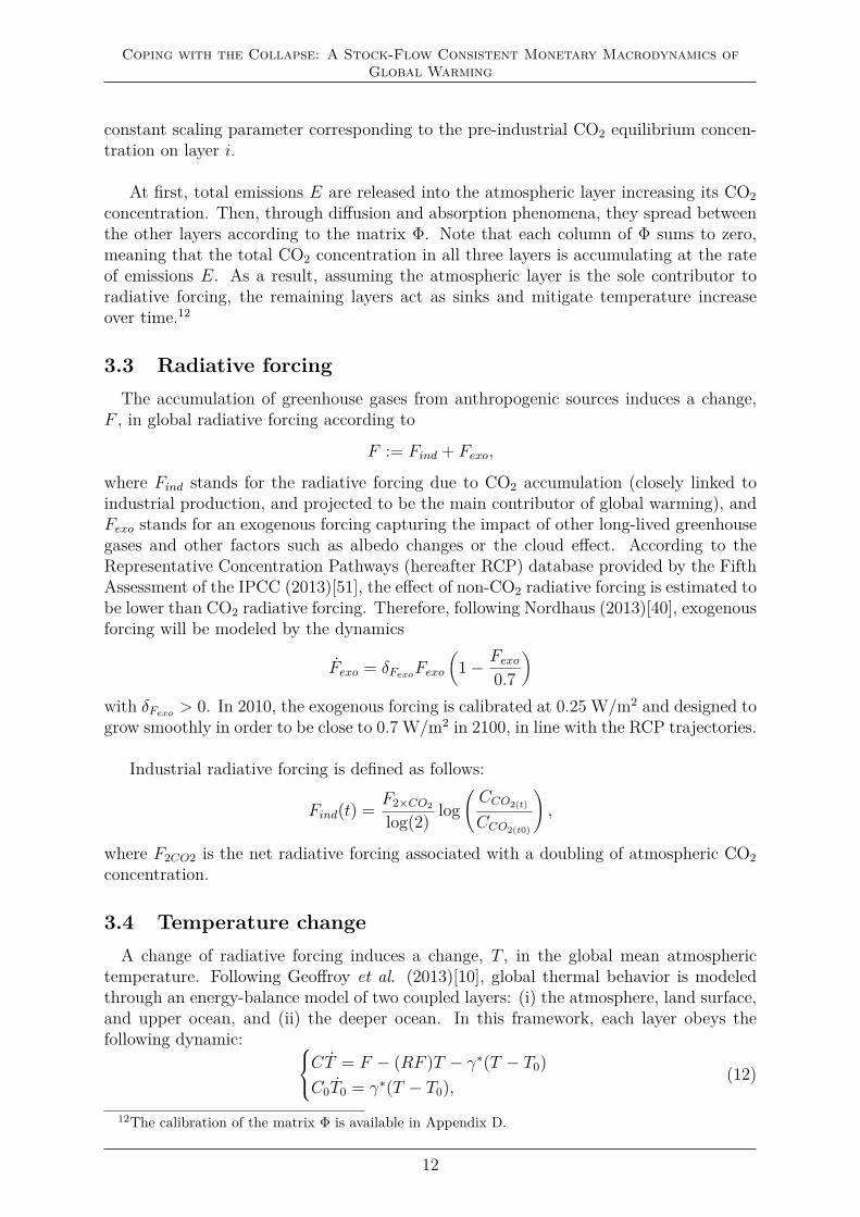
3.4 Temperature changeA change of radiative forcing induces a change, T , in the global mean atmospheric
temperature. Following Geoffroy et al. (2013)[10], global thermal behavior is modeledthrough an energy-balance model of two coupled layers: (i) the atmosphere, land surface,and upper ocean, and (ii) the deeper ocean. In this framework, each layer obeys thefollowing dynamic: CT = F − (RF )T − γ∗(T − T0)
C0T0 = γ∗(T − T0),(12)
12The calibration of the matrix Φ is available in Appendix D.
12

Coping with the Collapse: A Stock-Flow Consistent Monetary Macrodynamics ofGlobal Warming
where F is the radiative forcing, RF is the radiative feedback parameter, γ∗ is the heatexchange coefficient, C is the heat capacity of the atmosphere, land surface and upperocean layer, C0 is the heat capacity of the deep ocean layer and T and T0 are the meantemperature perturbation (deviation from the 1900 value) of respectively the atmosphere,land surface and upper ocean layer, and the deep ocean layer. The long-run equilibriumof the temperature anomaly is given by T = F/RF and will control the climate sensitivityas in Dietz-Stern (2015)[6].13
3.5 Climatic damagesFor our baseline scenario, we rely on the quadratic form of the damage function pro-
posed by Nordhaus (2013)[39]:
D = 1− 11 + π1T + π2T 2 ,
with π1 = 0, π2 = 2.84 × 10⁻³. Initially, the function relied on various sectoral studiessuch as crop losses or change in energy demand for space cooling or heating for severalpoints of global warming. It was then aggregated to describe the global impact of globalwarming based on the estimates of Tol (2009)[52]. This damage function is explicitlydesigned to model the effects of a global warming contained within a range of 0◦C to 3◦C.No threshold effects are thus allowed in this scenario after a temperature anomaly above3◦C.
3.6 Abatement costsAs public policy instruments are deployed, carbon emission abatement is achieved with
a cost, GY , partly borne by investment at the rate µ.14 The ratio, G, of abatement costto real output is defined by the following relation:
G = θ1nθ2 ,
where n stands for the rate of emissions reduction, defined shortly, and θ1, θ2 > 0. Here,θ2 > 0 is calibrated so that the abatement-cost-to-output ratio is highly convex.
The dynamics of abatement costs is linked to a backstop technology with a pricepBS and able replace carbon-intensive technology, and to a carbon price instrument pC .15
These prices follow exogenous trajectories defined by
pBSpBS
= δpBS < 0,
pCpC
= δpC > 0.16
13The calibration of the system (12) is available in Appendix B.14For the sake of completeness, the remaining part, (1− µ), is borne by households.15This price refers to the price per ton of CO2.16A sensitivity analysis will be provided. First, we use the same baseline as in Nordhaus et al.
(2013)[40]. The next scenarios, based on Nordhaus et al. (2013)[40] and Dietz and Stern (2015)[6],will be calibrated so that the growth parameter δpC
and the intial value of PC is in line with the optimalvalues reported in 2020 and 2050 (resp. 2015 and 2055), defined shortly.
13

Coping with the Collapse: A Stock-Flow Consistent Monetary Macrodynamics ofGlobal Warming
The reduction rate reflects an arbitrage relation between the relative prices of carbonand of the backstop technologies respectively,
n := min
(pcpBS
) 1θ2−1
; 1
.The parameter, θ1, reflects the cost of investing in the backstop technology through
its price and the carbon intensity of the economy. The parameters θ1, θ2 are calibratedaccording to Nordhaus (2013)[40]. Whenever pc ≥ pBS, the energy shift is completed.
Having described all the ingredients of our model, we are now ready to analyze thescenarios resulting from the interaction between global warming and debt accumulation.
4 ScenariosUsing the calibration depicted supra, we are now ready to discuss four main classes
of narratives that depend on labor productivity growth scenarios and previously defineddamage functions. The baseline case, the influence of each specification, and finally somecombinations are successively analyzed. For each scenario, the initial point is the year2010 and the simulations run until 2300, unless a collapse occurs before the final modelperiod.
4.1 Exponential technological progressFor the baseline case, we begin with an exogenous technological progress dynamic.
Labor productivity is assumed to grow at a constant rate:
a
a:= α > 0. (13)
For our simulations, we shall adopt two values for α: either 0.0226 or 0.015. The first isbased on an observed trend of technological progress at the world level.17 The second is aproxy of the parameterization adopted in Nordhaus (2013)[40]. Table 2 presents the mainparameters of our baseline simulation, obtained in the “exponential case” α = 0.0226, asspecified in Appendix (E.2). Monetary values are in US$ trillions. The population sizeis in billions. The GDP deflator (price level) is normalized to 1 in 2010. As already said,the short-run interest rate, r, is kept constant at 3%.
Parameter Y2010 N2010 ω2010 λ2010 d2010 p2010 αValue 64.4565 4.5510 0.5849 0.6910 1.4393 1 0.0226
Table 2: Main macroeconomic parameters of the exponential case
Figure 2 presents the deterministic exponential trajectories of our main macroeco-nomic and climate variables. After some fluctuations, the world economy reaches a stablepath with a finite debt ratio and stable inflation (roughly 2%). Yet, due to high emis-sions of CO2 (up to approximately 147.34 Gt CO2 in 2100), the temperature increases
17See details in Appendix E.2.
14

Coping with the Collapse: A Stock-Flow Consistent Monetary Macrodynamics ofGlobal Warming
(3.95◦C in 2100 in the atmospheric layer) and thus augments damages to production. Asa consequence, in the (ω, λ, d)-space represented in Figure 4, the wage share, ω, and theemployment rate, λ, slowly decrease. Then, as the energy shift reaches completion a littlebefore 2250, CO2 concentration, and thus damages, decrease.
0,00
0,01
0,02
0,03
0,04
0,05
0,0
0,2
0,4
0,6
0,8
1,0
2000 2050 2100 2150 2200 2250 2300
Employment RateInflation Rate (right axis)
-2
0
2
4
-0,03
-0,01
0,01
0,03
0,05
2000 2050 2100 2150 2200 2250 2300
Real Ouput GrowthLabor Productivity GrowthPopulation GrowthDebt to Nominal GDP Ratio (right axis)
0
5
10
15
20
25
0
15 000
30 000
45 000
60 000
75 000
2000 2050 2100 2150 2200 2250 2300
Real Output in $ 2010Emissions per Capita in tCO2 (right axis)
0,0
0,2
0,4
0,6
0,8
1,0
0
2
4
6
8
10
2000 2050 2100 2150 2200 2250 2300
Atmospheric Temperature Change in °CDamage to Real Output Ratio (right axis)
Figure 2: Trajectories of the main simulation outputs in the exponential case.
This baseline scenario yields important takeaways. First, as could be expected, de-terministic exponential productivity growth successfully drives the exponential growthof real GDP, despite climate damages. In 2100, it reaches 11.5 times its initial volumein 2010. This uninterrupted growth is accompanied by monetary and real cycles with aperiodicity of 12-17 years. This is consistent with the celebrated Kuznets swings, whichhave been recently re-examined by Korotayev and Tsirel (2010)[26]. However, as timepasses, these cycles seem to shorten during the first half of the twenty-second century.Ultimately, all volatility vanishes. Such a secular “Great Moderation” means that theglobal dynamical system is converging towards a long-run equilibrium where the em-ployment rate stabilizes around a comfortable 72% ratio, while the real output growthrate converges slightly above 2%. The (private nonfinancial corporate) debt-to-GDP ra-tio reaches a maximum in the middle of the twenty-second century (around 1.7) beforedeclining towards 142%.
15

Coping with the Collapse: A Stock-Flow Consistent Monetary Macrodynamics ofGlobal Warming
0,68
0,69
0,70
0,71
0,72
0,73
0,74
0,75
0,76
0,52 0,54 0,56 0,58 0,60 0,62 0,64 0,66
Em
plo
ym
ent
rate
Wage share
Figure 3: Phase diagram of employment rate vs. wage share in the exponential case overthe period 2010-2900.
As a consequence of the rise in CO2 concentration, the state of the world economy,illustrated by the phase portrait (ω, λ) in Figure 3, first deviates from its long-run equi-librium point. This temporary deviation reflects the impact of damages on the long-runequilibrium and especially on the wage share. Indeed, from 2100 until the energy shiftis completed, the rise in damage, D, is at its highest. At the same time, the wage sharedeclines in line with equation 10; so does inflation. Hence, higher profits lead the debtratio to stagnate before declining. In the aftermath of the transition to clean energy, theprivate debt-to-GDP ratio stagnates towards a long-run equilibrium level while damagesstart a downward-sloping trend.
Employment
Rate
Debt to
Nominal GDP
Ratio
Wage
Share
0,68
0,7
0,72
0,74
0,54
0,57
0,6
0,63
1,26
1,35
1,44
1,53
1,62
Figure 4: Phase diagram of employment rate vs. wage share and debt ratio in theexponential case.
As shown by the three-dimensional phase diagram in Figure 4, the (ω,λ)-plane firstconverges towards some equilibrium point close to (0.61, 0.72). But, soon after 2150, the
16

Coping with the Collapse: A Stock-Flow Consistent Monetary Macrodynamics ofGlobal Warming
wage share shifts towards 0.55. This departure from the long-run stationary state of theworld economy is only temporary, and entirely caused by climate change. Indeed, furthersimulations up to the year 2900 presented in Figure 3 show that, from the twenty-fourthcentury on, the state of the economy slowly reverts to the long-term equilibrium justalluded to.
This first scenario offers a quite reassuring picture in the time scale of the century.By 2050, as shown in Table 3, the average yearly CO2 emission per capita is 7.72t. Thetemperature change in 2100 is +3.94◦C and CO2 concentration, 968.98 ppm. Despitethe fact that we are far above the goal unanimously adopted at the Paris Agreement in2015, the world economy is going pretty well: the damages induced by global warmingreduce the final world real GDP by one fifth – a fraction higher than the 5% losses firstenvisaged by Stern (2006)[48] but this is seemingly easily counterbalanced by the strengthof the postulated exogenous growth. As a result of this quite unrealistic picture, CO2emissions peak only in the middle of the twenty-second century and the zero-emissionlevel is reached one century later!
GDP Real Growth 2100 (wrt 2010) 1053%t CO2 per capita (2050) 7.72Temperature change in 2100 +3.94 ◦CCO2 concentration 2100 968.98 ppm
Table 3: Key values of the world economy by 2100 – the exogenous case.
By exhibiting a relatively low impact of damages and negligible abatement costs (lessthan 1% of real output) for production by 2100 or so, this scenario above all confirms theunrealistic feature of the climate-economy interaction modeling on which it is based. Aswe shall now see, the picture changes dramatically as soon as labor productivity is madeendogenous.18
4.2 Endogenous productivityLet us now discuss alternative scenarios of endogenous labor productivity growth com-
bined with the damage function introduced by Nordhaus (2013)[40].
4.2.1 The Kaldor-Verdoorn case
The Kaldor-Verdoorn case assumes a relationship between labor productivity growthand output growth (cf. Verdoorn (2002)[56]) in the form
a
a:= α + ηg, (14)
with g being the real output growth, and α, η > 0. Equation 14 can be interpreted asreflecting dynamic economies of scale (or “learning by doing”). A rough estimate forthe United States over the last four decades is α ' 0 and η ' 0.5, with a tendency
18For the sake of comparison with DICE, the “Nordhaus scenario”, and Gordon (2014)[16] – wherelabor productivity grows approximately at the deterministic pace of 1.5% and 1.3% respectively – arediscussed in the supplementary web material. The findings are qualitatively similar to the ones justdescribed.
17

Coping with the Collapse: A Stock-Flow Consistent Monetary Macrodynamics ofGlobal Warming
of both parameters to increase due to the impact of Information and CommunicationTechnologies. In our simulations, we assume equation 14 to hold at the world level. Thiswill be considered optimistic or pessimistic depending on how strongly one believes thatthe opportunity for emerging economies to follow a learning process analogous to therecent trend in the United States is realistic or not.
0,00
0,01
0,02
0,03
0,04
0,05
0,06
0,0
0,2
0,4
0,6
0,8
1,0
2000 2050 2100 2150 2200 2250 2300
Employment RateInflation Rate (right axis)
-2
0
2
4
-0,03
-0,01
0,01
0,03
0,05
2000 2050 2100 2150 2200 2250 2300
Real Ouput GrowthLabor Productivity GrowthPopulation GrowthDebt to Nominal GDP Ratio (right axis)
0
2
4
6
8
0
20
40
60
80
100
120
2000 2050 2100 2150 2200 2250 2300
Real Output in $ 2010Emissions per Capita in tCO2 (right axis)
0,0
0,2
0,4
0,6
0,8
1,0
0
1
2
3
4
5
6
7
2000 2050 2100 2150 2200 2250 2300
Atmospheric Temperature Change in °CDamage to Real Output Ratio (right axis)
Figure 5: Trajectories in the Kaldor-Verdoorn/Nordhaus case.
Figure 5 depicts the path followed by the world economy in the Kaldor-Verdoornscenario. By contrast with the previous pattern, the economy converges to a stationarystate with stagnating labor productivity and no real output growth. This “millennialstagnation” starts at the end of this century and is accompanied by a debt ratio andinflation rate higher than in the exponential case. Carbon emissions decline almost im-mediately after 2010. The zero emission floor is reached before the second half of thetwenty-second century.
0,67
0,68
0,69
0,70
0,71
0,72
0,73
0,74
0,75
0,76
0,77
0,55 0,60 0,65 0,70 0,75 0,80
Em
plo
ym
ent
rate
Wage share
Figure 6: Phase diagram of employment rate vs. wage share in the Kaldor-Verdoorn/Nordhaus case.
18
Coping with the Collapse: A Stock-Flow Consistent Monetary Macrodynamics ofGlobal Warming
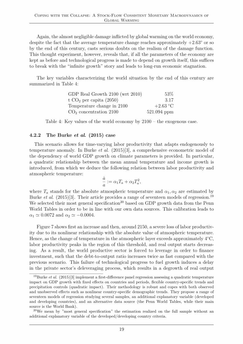
Again, the almost negligible damage inflicted by global warming on the world economy,despite the fact that the average temperature change reaches approximately +2.63◦ or soby the end of this century, casts serious doubts on the realism of the damage function.This thought experiment, however, reveals that, if all the parameters of the economy arekept as before and technological progress is made to depend on growth itself, this sufficesto break with the “infinite growth” story and leads to long-run economic stagnation.
The key variables characterizing the world situation by the end of this century aresummarized in Table 4:
GDP Real Growth 2100 (wrt 2010) 53%t CO2 per capita (2050) 3.17Temperature change in 2100 +2.63 ◦CCO2 concentration 2100 521.094 ppm
Table 4: Key values of the world economy by 2100 – the exogenous case.
4.2.2 The Burke et al. (2015) case
This scenario allows for time-varying labor productivity that adapts endogenously totemperature anomaly. In Burke et al. (2015)[3], a comprehensive econometric model ofthe dependency of world GDP growth on climate parameters is provided. In particular,a quadratic relationship between the mean annual temperature and income growth isintroduced, from which we deduce the following relation between labor productivity andatmospheric temperature:
a
a:= α1Ta + α2T
2a ,
where Ta stands for the absolute atmospheric temperature and α1, α2 are estimated byBurke et al. (2015)[3]. Their article provides a range of seventeen models of regression.19
We selected their most general specification20 based on GDP growth data from the PennWorld Tables in order to be in line with our own data sources. This calibration leads toα1 ' 0.0072 and α2 ' −0.0004.
Figure 7 shows first an increase and then, around 2150, a severe loss of labor productiv-ity due to its nonlinear relationship with the absolute value of atmospheric temperature.Hence, as the change of temperature in the atmospheric layer exceeds approximately 4◦C,labor productivity peaks in the region of this threshold, and real output starts decreas-ing. As a result, the world productive sector is forced to leverage in order to financeinvestment, such that the debt-to-output ratio increases twice as fast compared with theprevious scenario. This failure of technological progress to fuel growth induces a delayin the private sector’s deleveraging process, which results in a degrowth of real output
19Burke et al. (2015)[3] implement a first-difference panel regression assessing a quadratic temperatureimpact on GDP growth with fixed effects on countries and periods, flexible country-specific trends andprecipitation controls (quadratic impact). Their methodology is robust and copes with both observedand unobserved effects such as nonlinear country-specific demographic trends. They propose a range ofseventeen models of regression studying several samples, an additional explanatory variable (developedand developing countries), and an alternative data source (the Penn World Tables, while their mainsource is the World Bank).
20We mean by ”most general specification” the estimation realized on the full sample without anadditional explanatory variable of the developed/developing country criteria.
19

Coping with the Collapse: A Stock-Flow Consistent Monetary Macrodynamics ofGlobal Warming
starting in the second half of the twenty-second century. In the vicinity of the modelyear 2135, world real GDP peaks at around 600% of its 2010 value, and then inexorablydeclines. As a counterpart, the debt-to-GDP ratio explodes: it is already above 250% by2100, and peaks slightly below 400% thereafter. Fortunately, emissions per capita havealready peaked around 2050, such that the temperature change in 2100 remains lowerthan in the exogenous-growth scenario (+4.92◦C).
0,00
0,01
0,02
0,03
0,04
0,05
0,0
0,2
0,4
0,6
0,8
1,0
2000 2050 2100 2150 2200 2250 2300
Employment RateInflation Rate (right axis)
-2
0
2
4
-0,03
-0,01
0,01
0,03
0,05
2000 2050 2100 2150 2200 2250 2300
Real Ouput GrowthLabor Productivity GrowthPopulation GrowthDebt to Nominal GDP Ratio (right axis)
0
2
4
6
8
0
100
200
300
400
2000 2050 2100 2150 2200 2250 2300
Real Output in $ 2010Emissions per Capita in tCO2 (right axis)
0,0
0,2
0,4
0,6
0,8
1,0
0
1
2
3
4
5
6
7
2000 2050 2100 2150 2200 2250 2300
Atmospheric Temperature Change in °CDamage to Real Output Ratio (right axis)
Figure 7: The Burke et al. labor productivity trajectory with the Nordhaus damagefunction.
The phase diagram in Figure 8 highlights the channel linking global warming, surplusdistribution, and growth. Indeed, as a consequence of equation 10, the deceleration oflabor productivity favors an increase in the wage share, lowering relative profits andforcing the private sector to increase its debt in order to compensate for profit losses.
0,68
0,69
0,70
0,71
0,72
0,73
0,74
0,75
0,76
0,54 0,56 0,58 0,60 0,62 0,64 0,66 0,68 0,70
Em
plo
ym
ent
rate
Wage share
Figure 8: Phase diagram in the Burke et al./Nordhaus case.
However, this “degrowth by constraint” (not by design) has no disruptive effect onthe labor market, since the employment rate converges around 70% at the end of this
20

Coping with the Collapse: A Stock-Flow Consistent Monetary Macrodynamics ofGlobal Warming
century. As for inflation, this is slightly higher than in the previous scenario but eventuallyconverges to a quite reasonable 3.5% in the second half of the twenty-third century. Noticealso that the damage function has very little impact in this scenario, as in the previousone, since the temperature anomaly peaks at around only 3.5◦C or so.
GDP Real Growth 2100 (wrt 2010) 397%t CO2 per capita in 2050 6.29Temperature change in 2100 +3.48 ◦CCO2 concentration in 2100 744.49 ppm
Table 5: The world economy by 2100 – the endogenous case with Nordhaus damagefunction.
Of course, forced degrowth at the world scale might seem an implausible patterngiven the impressively innovative character of advanced economies (think of the ICTrevolution) and the quite impressive growth experienced by emerging countries in recentdecades. Remember, however, that during the 1990s the former Soviet Union experienceda 50% reduction of its GDP within one decade, while Greece lost 25% of its GDP between2010 and 2015. Undesired degrowth is not therefore a fictional phenomenon.
Thus far, we have kept the damage function identical and discussed the sensitivity ofour prospective paths with respect to various specifications of technological progress. Letus now proceed the other way round and test various damage functions while keeping adeterministic exponential labor productivity growth.
4.3 Assessing the impact of climate changeSo far, there is no academic consensus on a functional formulation and calibration of
the damage function capturing the impact of climate on the world economy. Indeed, aspointed out by Pindyck (2015)[41], no theory and no data exist on which such a consensuscould be reliably grounded. On the other hand, this function has to summarize theeconomic impacts, as a percentage of output, brought on by the rise in mean atmospherictemperature. It thus has to compile a wide range of events such as biodiversity loss, oceanacidification, sea-level rise, change in ocean circulation, and high-frequency storms, amongothers. As a consequence, the damage function is highly nonlinear with threshold effects.In this section, various damage functions will be considered. We keep labor productivityat the somewhat high growth rate of 2.26%, so that the only difference with the BAUscenario analyzed supra lies in our assessment of climatic damages.
As argued by Dietz and Stern (2015)[6], Nordhaus’ quadratic form leads to unrealis-tically low damages beyond a temperature increase of 4◦C. For instance, a global warmingof 4◦C would lead to only 4% of output loss whereas, according to natural science andeconomic studies, reaching this threshold could be a milestone. On the one hand, Lentonet al. (2008)[28] point out that several key tipping points in the climate system could becrossed and lead to severe impacts on the natural environment. On the other hand, Stern(2013)[49] shows that this situation would generate large migrations associated with con-flict and loss of life. Our simulations in the next section will unfortunately confirm thiscriticism.
21
Coping with the Collapse: A Stock-Flow Consistent Monetary Macrodynamics ofGlobal Warming
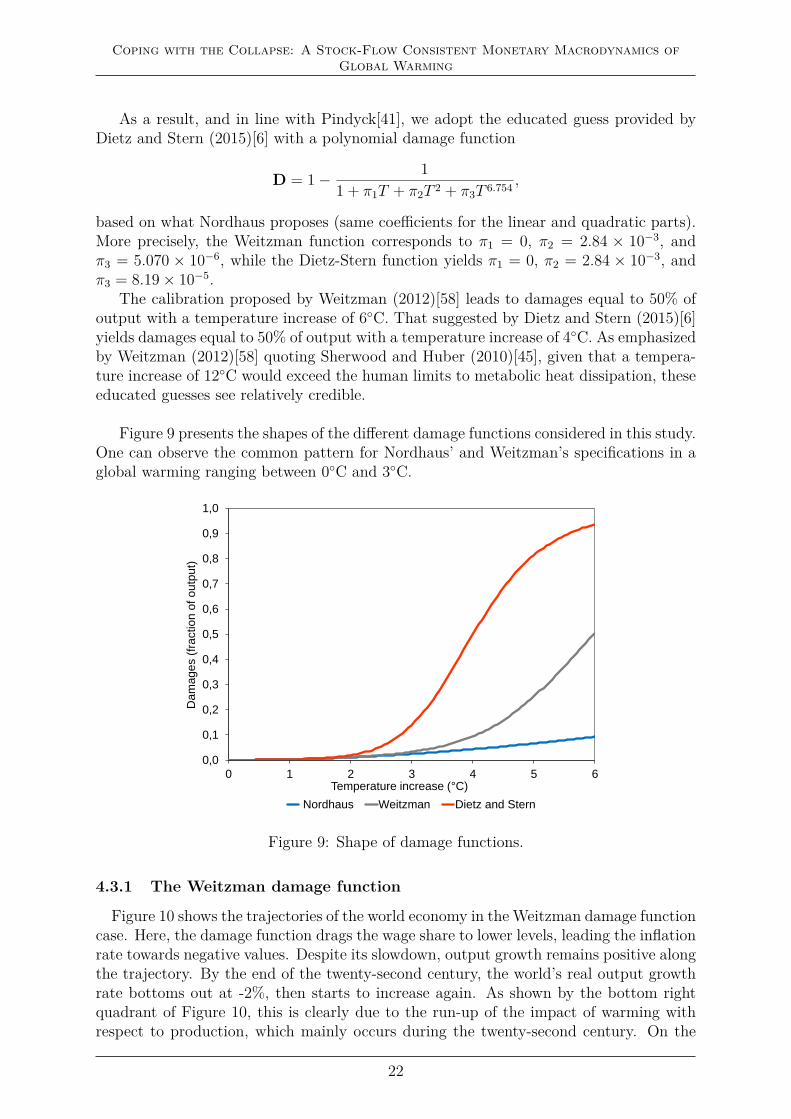
As a result, and in line with Pindyck[41], we adopt the educated guess provided byDietz and Stern (2015)[6] with a polynomial damage function
D = 1− 11 + π1T + π2T 2 + π3T 6.754 ,
based on what Nordhaus proposes (same coefficients for the linear and quadratic parts).More precisely, the Weitzman function corresponds to π1 = 0, π2 = 2.84 × 10⁻³, andπ3 = 5.070 × 10⁻⁶, while the Dietz-Stern function yields π1 = 0, π2 = 2.84 × 10⁻³, andπ3 = 8.19× 10⁻⁵.
The calibration proposed by Weitzman (2012)[58] leads to damages equal to 50% ofoutput with a temperature increase of 6◦C. That suggested by Dietz and Stern (2015)[6]yields damages equal to 50% of output with a temperature increase of 4◦C. As emphasizedby Weitzman (2012)[58] quoting Sherwood and Huber (2010)[45], given that a tempera-ture increase of 12◦C would exceed the human limits to metabolic heat dissipation, theseeducated guesses see relatively credible.
Figure 9 presents the shapes of the different damage functions considered in this study.One can observe the common pattern for Nordhaus’ and Weitzman’s specifications in aglobal warming ranging between 0◦C and 3◦C.
0,0
0,1
0,2
0,3
0,4
0,5
0,6
0,7
0,8
0,9
1,0
0 1 2 3 4 5 6
Da
mages (
fraction o
f outp
ut)
Temperature increase (°C)
Nordhaus Weitzman Dietz and Stern
Figure 9: Shape of damage functions.
4.3.1 The Weitzman damage function
Figure 10 shows the trajectories of the world economy in the Weitzman damage functioncase. Here, the damage function drags the wage share to lower levels, leading the inflationrate towards negative values. Despite its slowdown, output growth remains positive alongthe trajectory. By the end of the twenty-second century, the world’s real output growthrate bottoms out at -2%, then starts to increase again. As shown by the bottom rightquadrant of Figure 10, this is clearly due to the run-up of the impact of warming withrespect to production, which mainly occurs during the twenty-second century. On the
22

Coping with the Collapse: A Stock-Flow Consistent Monetary Macrodynamics ofGlobal Warming
other hand, the wage share, ω, stays below 35% until the end of the same century, implyinghigh profits and the beginning of an age of deleveraging and even excess saving.21
-0,07
-0,05
-0,03
-0,01
0,01
0,03
0,05
0,0
0,2
0,4
0,6
0,8
1,0
2000 2050 2100 2150 2200 2250 2300
Employment RateInflation Rate (right axis)
-2
0
2
4
-0,03
-0,01
0,01
0,03
0,05
2000 2050 2100 2150 2200 2250 2300
Real Ouput GrowthLabor Productivity GrowthPopulation GrowthDebt to Nominal GDP Ratio (right axis)
0
2
4
6
8
10
12
14
0
200
400
600
800
1 000
1 200
1 400
1 600
2000 2050 2100 2150 2200 2250 2300
Real Output in $ 2010Emissions per Capita in tCO2 (right axis)
0,0
0,2
0,4
0,6
0,8
1,0
0
1
2
3
4
5
6
7
2000 2050 2100 2150 2200 2250 2300
Atmospheric Temperature Change in °CDamage to Real Output Ratio (right axis)
Figure 10: Trajectories of the main simulation outputs in the exponential/Weitzman case.
The phase portrait in Figure 11 highlights the decline of the wage share, while the em-ployment rate steadily decreases to around 0. The fact that the world economy managesto produce some positive output growth in the second half of the twenty-third century,even though its employment rate is close to nil, confirms the unrealistic feature of ourpostulated exogenous growth rate of labor productivity.
0,00
0,10
0,20
0,30
0,40
0,50
0,60
0,70
0,80
0,00 0,10 0,20 0,30 0,40 0,50 0,60 0,70
Em
plo
ym
ent
rate
Wage share
Figure 11: Phase diagram of employment rate vs. wage share in the exponen-tial/Weitzman case.
21It is worth mentioning that the empirical estimation of investment, κ(·), as a function of the profitrate, π, is silent about domains where π has so far not been observed. This hardly surprising: climatechange will necessarily lead the world economy to explore situations for which no data can be borrowedfrom the past. It does however raise a question: which values should be given to investment when π isabnormally high or low? Here, we have capped and floored κ(·) between 50% and 4% of real output.
23

Coping with the Collapse: A Stock-Flow Consistent Monetary Macrodynamics ofGlobal Warming
GDP Real Growth 2100 (wrt 2010) 987%t CO2 per capita in 2050 7.72Temperature change in 2100 +3.93 ◦CCO2 concentration in 2100 958.17 ppm
Table 6: The world economy by 2100 – the exogenous case with Weitzman damages.
4.3.2 Damages a la Dietz-Stern
Let us now adopt the probably more realistic Dietz-Stern damage function. Figure12 shows its impact on the main macroeconomic and climate variables. Qualitatively,the short run exhibits a pattern similar to the previous scenario. Quantitatively, realGDP is more muted. In the previous scenario, it peaked in the region of (2010) US$1400 trillion around 2175, whereas in the current scenario the highest point is reachedin 2100 at slightly above US$ 400 trillion. This more severe picture leads to a real GDPthat is lower in 2175 than in 2010. In this scenario, damages absorb more than 60%of real output as the temperature increase in the upper atmosphere reaches 4◦C around2125. For the sake of comparison, at that date in the previous scenario “only” 20% ofthe world’s real output was destroyed by global warming. Finally, the debt-to-GDP ratiospikes at around 250% towards 2125, whereas in the Weitzman case it stood below 200%for the same period. A more severe damage function reinforces the run-up to debt duringthe period when the economy is still growing. Note that, as previously, a deleveragingperiod starts whenever GDP decreases.
-0,07
-0,05
-0,03
-0,01
0,01
0,03
0,05
0,0
0,2
0,4
0,6
0,8
1,0
2000 2050 2100 2150 2200 2250 2300
Employment RateInflation Rate (right axis)
-2
0
2
4
-0,03
-0,01
0,01
0,03
0,05
2000 2050 2100 2150 2200 2250 2300
Real Ouput GrowthLabor Productivity GrowthPopulation GrowthDebt to Nominal GDP Ratio (right axis)
0
2
4
6
8
10
12
14
0
100
200
300
400
500
2000 2050 2100 2150 2200 2250 2300
Real Output in $ 2010Emissions per Capita in tCO2 (right axis)
0,0
0,2
0,4
0,6
0,8
1,0
0
1
2
3
4
5
6
7
2000 2050 2100 2150 2200 2250 2300
Atmospheric Temperature Change in °CDamage to Real Output Ratio (right axis)
Figure 12: The exponential/Dietz-Stern case.
24
Coping with the Collapse: A Stock-Flow Consistent Monetary Macrodynamics ofGlobal Warming
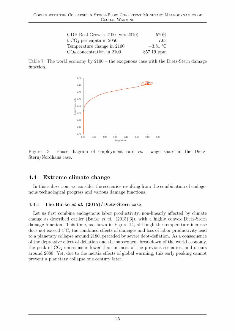
GDP Real Growth 2100 (wrt 2010) 520%t CO2 per capita in 2050 7.63Temperature change in 2100 +3.81 ◦CCO2 concentration in 2100 857.19 ppm
Table 7: The world economy by 2100 – the exogenous case with the Dietz-Stern damagefunction.
0,00
0,10
0,20
0,30
0,40
0,50
0,60
0,70
0,80
0,00 0,10 0,20 0,30 0,40 0,50 0,60 0,70
Em
plo
ym
ent
rate
Wage share
Figure 13: Phase diagram of employment rate vs. wage share in the Dietz-Stern/Nordhaus case.
4.4 Extreme climate changeIn this subsection, we consider the scenarios resulting from the combination of endoge-
nous technological progress and various damage functions.
4.4.1 The Burke et al. (2015)/Dietz-Stern case
Let us first combine endogenous labor productivity, non-linearly affected by climatechange as described earlier (Burke et al. (2015)[3]), with a highly convex Dietz-Sterndamage function. This time, as shown in Figure 14, although the temperature increasedoes not exceed 4◦C, the combined effects of damages and loss of labor productivity leadto a planetary collapse around 2180, preceded by severe debt-deflation. As a consequenceof the depressive effect of deflation and the subsequent breakdown of the world economy,the peak of CO2 emissions is lower than in most of the previous scenarios, and occursaround 2080. Yet, due to the inertia effects of global warming, this early peaking cannotprevent a planetary collapse one century later.
25

Coping with the Collapse: A Stock-Flow Consistent Monetary Macrodynamics ofGlobal Warming
-0,07
-0,05
-0,03
-0,01
0,01
0,03
0,05
0,0
0,2
0,4
0,6
0,8
1,0
2000 2020 2040 2060 2080 2100 2120 2140 2160 2180
Employment RateInflation Rate (right axis)
-10
-5
0
5
10
15
20
-0,03
-0,01
0,01
0,03
0,05
2000 2020 2040 2060 2080 2100 2120 2140 2160 2180
Real Ouput GrowthLabor Productivity GrowthPopulation GrowthDebt to Nominal GDP Ratio (right axis)
0
2
4
6
8
0
50
100
150
200
250
2000 2020 2040 2060 2080 2100 2120 2140 2160 2180
Real Output in $ 2010Emissions per Capita in tCO2 (right axis)
0,0
0,2
0,4
0,6
0,8
1,0
0
1
2
3
4
5
6
7
2000 2020 2040 2060 2080 2100 2120 2140 2160 2180
Atmospheric Temperature Change in °CDamage to Real Output Ratio (right axis)
Figure 14: The Burke et al. (2015)/Dietz-Stern case.
0,00
0,10
0,20
0,30
0,40
0,50
0,60
0,70
0,80
0,00 0,10 0,20 0,30 0,40 0,50 0,60 0,70
Em
plo
ym
ent
rate
Wage share
Figure 15: Phase diagram of employment rate vs. wage share in the Burke et al./Dietz-Stern case.
4.4.2 The Burke et al. (2015)/Dietz-Stern case with a slower demographictrend
Could a deceleration of the demographic trend prevent a disaster? This subsectionprovides some elements for an answer by assuming the demographic trend to be slowerthan in the UN median scenario within the Burke et al. labor productivity growth case,together with the Dietz-Stern damage function previously presented. For this purpose,we divide by four the speed of convergence, q, but we keep the same upper bound forthe dynamics of the labor force, M . Figure 16 offers a comparison of the demographicscenarios.
26

Coping with the Collapse: A Stock-Flow Consistent Monetary Macrodynamics ofGlobal Warming
4,0
4,5
5,0
5,5
6,0
6,5
7,0
7,5
2000 2050 2100 2150 2200 2250
Billion o
f w
ork
ers
Calibrated speed of convergence Slower speed of convergence
Figure 16: Comparison of the labor-force demographic trajectories.
According to our altered demographic scenario, the world’s working-age populationwould be approximately 5 billion people in 2100, instead of 7 billion as in the UN me-dian projection. Figure 17 shows the paths followed by the world economy in this case.Despite lower CO2 emissions, we observe patterns analogous to those obtained in theoriginal Burke/Dietz-Stern case, leading to a global collapse around the model year 2240.The main difference between the two narratives lies in the speed at which events occur:the second narrative exhibits a 4–5-decade delay relative to the first. This suggests thata downturn in the demographic trend does not suffice per se to avoid a disaster, but itnevertheless manages to postpone it for a few decades.
Unfortunately, other simulations, even with no population growth,22 show that in theBurke/Dietz-Stern case a global collapse always occurs whatever the population trend.Even in the utterly unrealistic case in which world population stays at its 2010 level,the intrinsic devastating forces arising from the combination of climate change and debtwould lead to a breakdown around 2400. In terms of public policy, this means thatsteering world population growth cannot be viewed as a panacea, but it does have apositive impact on the global economic calendar of our planet.
22These simulations are available from the authors upon request.
27

Coping with the Collapse: A Stock-Flow Consistent Monetary Macrodynamics ofGlobal Warming
-0,07
-0,05
-0,03
-0,01
0,01
0,03
0,05
0,0
0,2
0,4
0,6
0,8
1,0
2000 2040 2080 2120 2160 2200 2240
Employment RateInflation Rate (right axis)
-10
-5
0
5
10
15
20
-0,03
-0,01
0,01
0,03
0,05
2000 2040 2080 2120 2160 2200 2240
Real Ouput GrowthLabor Productivity GrowthPopulation GrowthDebt to Nominal GDP Ratio (right axis)
0
2
4
6
8
0
50
100
150
200
250
2000 2040 2080 2120 2160 2200 2240
Real Output in $ 2010Emissions per Capita in tCO2 (right axis)
0,0
0,2
0,4
0,6
0,8
1,0
0
1
2
3
4
5
6
7
2000 2040 2080 2120 2160 2200 2240
Atmospheric Temperature Change in °CDamage to Real Output Ratio (right axis)
Figure 17: Trajectories of the main simulation outputs for the case with the Burkeet al. (2015) labor productivity growth, a Dietz-Stern damage function, and a slowerdemographic trend.
4.5 Carbon prices and climate sensitivitySince demography alone does not suffice to circumvent the potentially disastrous effects
of global warming, we now turn to the carbon value. So far, we have considered thebaseline scenario of the carbon price introduced by Nordhaus (2013)[40]. For the sake ofclarity, the price of the t/CO2 in (2005) $US is one in 2010 and grows steadily by twopercent per year.
In this section, we retain the Burke et al. (2015)[3] labor productivity dynamic cou-pled with a Dietz-Stern damage function, but modify the carbon price path, takinginspiration from Dietz and Stern (2015)[6]. On the demographic side, we again adoptthe UN median projection, as we do throughout this paper except for Section 4.4.2 above.
4.5.1 Dietz and Stern’s standard-run
We now assume that the carbon price follows the path examined in Dietz and Stern(2015)[6], starting with (2005) $US 12 t/CO2 in 2015 and reaching $US 29 t/CO2 in2055.
28
Coping with the Collapse: A Stock-Flow Consistent Monetary Macrodynamics ofGlobal Warming
0,00
0,01
0,02
0,03
0,04
0,05
0,0
0,2
0,4
0,6
0,8
1,0
2000 2050 2100 2150 2200 2250 2300
Employment RateInflation Rate (right axis)
-2
0
2
4
-0,03
-0,01
0,01
0,03
0,05
2000 2050 2100 2150 2200 2250 2300
Real Ouput GrowthLabor Productivity GrowthPopulation GrowthDebt to Nominal GDP Ratio (right axis)
0
1
2
3
4
5
6
0
200
400
600
800
1 000
1 200
2000 2050 2100 2150 2200 2250 2300
Real Output in $ 2010Emissions per Capita in tCO2 (right axis)
0,0
0,2
0,4
0,6
0,8
1,0
0
1
2
3
4
5
6
7
2000 2050 2100 2150 2200 2250 2300
Atmospheric Temperature Change in °CDamage to Real Output Ratio (right axis)
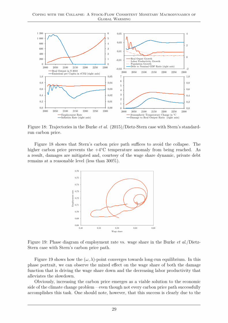
Figure 18: Trajectories in the Burke et al. (2015)/Dietz-Stern case with Stern’s standard-run carbon price.
Figure 18 shows that Stern’s carbon price path suffices to avoid the collapse. Thehigher carbon price prevents the +4◦C temperature anomaly from being reached. Asa result, damages are mitigated and, courtesy of the wage share dynamic, private debtremains at a reasonable level (less than 300%).
0,68
0,69
0,70
0,71
0,72
0,73
0,74
0,75
0,76
0,48 0,53 0,58 0,63 0,68
Em
plo
ym
ent
rate
Wage share
Figure 19: Phase diagram of employment rate vs. wage share in the Burke et al./Dietz-Stern case with Stern’s carbon price path.
Figure 19 shows how the (ω, λ)-point converges towards long-run equilibrium. In thisphase portrait, we can observe the mixed effect on the wage share of both the damagefunction that is driving the wage share down and the decreasing labor productivity thatalleviates the slowdown.
Obviously, increasing the carbon price emerges as a viable solution to the economicside of the climate change problem – even though not every carbon price path successfullyaccomplishes this task. One should note, however, that this success is clearly due to the
29

Coping with the Collapse: A Stock-Flow Consistent Monetary Macrodynamics ofGlobal Warming
utterly simple, and probably unrealistic, way we model the world economy’s shift from acurrent energy mix comprising 80% of fossil energies towards a zero-carbon economy.
4.5.2 Dietz and Stern’s standard-run with a climate Sensitivity of 6
So far, all our results are based on a climate sensitivity whereby a doubling in the atmo-spheric concentration of CO2 translates into a +2.9◦C rise relative to the pre-industrialera. This value reflects the mean of a Pareto distribution whose tail yields a 6% like-lihood that a rise of +6◦C or more will occur in these circumstances (see Weitzman(2011)[57]). We thus test some of our scenarios under a climate sensitivity of 6, ratherthan 2.9. Clearly, in this setting, any variation of CO2 will lead to a higher response intemperature anomaly compared to its +2.9◦C counterpart.
We begin with the most problematic scenario examined thus far, namely that insubsection 4.4.1 supra, which combines an endogenous labor productivity a la Burkeet al.(2015) and a highly convex Dietz-Stern damage function. At variance with thesituation envisaged in the subsection just mentioned, here, we keep the carbon price pathintroduced by Stern (instead of relying on Nordhaus’s price path as in section 4.4.1).
-0,07
-0,05
-0,03
-0,01
0,01
0,03
0,05
0,0
0,2
0,4
0,6
0,8
1,0
2000 2020 2040 2060 2080 2100 2120
Employment RateInflation Rate (right axis)
-10
-5
0
5
10
15
20
-0,03
-0,01
0,01
0,03
0,05
2000 2020 2040 2060 2080 2100 2120
Real Ouput GrowthLabor Productivity GrowthPopulation GrowthDebt to Nominal GDP Ratio (right axis)
0
1
2
3
4
5
6
0
50
100
150
200
2000 2020 2040 2060 2080 2100 2120
Real Output in $ 2010Emissions per Capita in tCO2 (right axis)
0,0
0,2
0,4
0,6
0,8
1,0
0
1
2
3
4
5
6
7
2000 2020 2040 2060 2080 2100 2120
Atmospheric Temperature Change in °CDamage to Real Output Ratio (right axis)
Figure 20: Trajectories in the Burke et al. (2015)/Dietz-Stern case with the standard-runprice of carbon and a climate sensitivity of 6.
Figure 20 shows that the preceding specification of the carbon price no longer avoids acollapse of the economy. The cap of a +4◦C temperature rise relative to the pre-industriallevel is reached long before 2100. Consequently, high damages together with the inertiaof CO2 in the atmospheric layer lead the world economy to deflation and a skyrocketingdebt ratio, yet again ending up in a global breakdown.
Next, we test the carbon price path more recently introduced by Dietz and Stern(2015)[6] for a climate sensitivity of 6 and a damage function a la Weitzman. Convertedinto 2005 $US, in 2015 the price of the ton of CO2 is now US$ 74, and US$ 306 in 2055.
30

Coping with the Collapse: A Stock-Flow Consistent Monetary Macrodynamics ofGlobal Warming
0,00
0,01
0,02
0,03
0,04
0,05
0,0
0,2
0,4
0,6
0,8
1,0
2000 2050 2100 2150 2200 2250 2300
Employment RateInflation Rate (right axis)
-2
0
2
4
-0,03
-0,01
0,01
0,03
0,05
2000 2050 2100 2150 2200 2250 2300
Real Ouput GrowthLabor Productivity GrowthPopulation GrowthDebt to Nominal GDP Ratio (right axis)
0
1
2
3
4
5
6
0
200
400
600
800
2000 2050 2100 2150 2200 2250 2300
Real Output in $ 2010Emissions per Capita in tCO2 (right axis)
0,0
0,2
0,4
0,6
0,8
1,0
0
1
2
3
4
5
6
7
2000 2050 2100 2150 2200 2250 2300
Atmospheric Temperature Change in °CDamage to Real Output Ratio (right axis)
Figure 21: Trajectories in the Burke et al. (2015)/Dietz-Stern case,the Dietz-Stern carbonprice path, and a climate sensitivity of 6.
This time, the carbon price path turns out to be sufficient to avoid the collapse.Figure 21 displays a trajectory in which real GDP in 2100 reaches about 2.72 times itsvalue in 2010, with the emission of t CO2 per capita decreasing to 0.70 in 2050 and thetemperature increasing to only +3.23◦C in 2100.
4.5.3 Objective +1.5◦C
The Paris Agreement of 2015 aims to keep the temperature anomaly below +2◦C anddrive efforts to stay as close as possible to a +1.5◦C threshold. Is such a target reachableaccording to the framework developed in this paper?
We base our analysis on the scenario that to us seems the most realistic we have con-sidered so far in this paper, namely the Burke et al. (2015)[3] labor productivity growthtogether with the Dietz and Stern (2015)[6] damage function. Within this framework, thedoubling in CO2 concentration implies a temperature anomaly of 6◦C (i.e., if the climatesensitivity is 6), while the increase in temperature turns out to be already about +1.52◦Cin 2100 even if CO2 emissions were to remain at their 2010 level. Thus, in our set-up,there is no hope of reaching the 1.5◦C target were the climate sensitivity equal to 6.
We therefore consider lower climate sensitivities ranging from 1.5 to 2.9. In thissetting, we test which carbon price path could prevent the temperature anomaly fromexceeding the +1.5◦C ceiling. For this, we use a constant initial condition for the carbonprice in 2010 (either US$ 15, or US$ 80) and look for the per annum growth parameterthat prevents the temperature anomaly from exceeding +1.5◦C in 2100.23
23We do not claim that the values obtained here are minimal (whatever the sense one might wish to givethis here) in order to reach the +1.5◦C target. At best, they are educated guesses given our numericalexperience with the present model. We believe, however, that they provide a faithful indication of whata more systematic exploration of this model’s sensitivity relative to the carbon price path would provide.The latter is left for further research.
31

Coping with the Collapse: A Stock-Flow Consistent Monetary Macrodynamics ofGlobal Warming
Sensitivity of +1.5◦C Sensitivity of +2.9◦CInit. price of 15 Init. price of 80 Init. price of 15 Init. price of 80
Price in 2015 18.58 86.27 65.50 144.32Price in 2020 23.00 93.04 286.02 260.35Price in 2050 82.93 146.35 xxx xxx
Table 8: Carbon prices preventing the temperature anomaly from reaching the 1.5◦Cceiling, in (2005) US$/tCO2.
Table 8 provides some carbon price paths that prevent the temperature anomaly fromexceeding the 1.5◦C ceiling. When xxx is reported, the simulated values are higher than2005 US$ 344 (the maximum price of the backstop technology, in the same currency unit,needed to complete the energy shift), and thus meaningless. As expected, prices need tobe higher in the 2.9 case than in the 1.5 case in order to reach the 1.5◦C target.
The 1.5◦C sensitivity case shows that the necessary carbon price increase is lowerwhen the initial price is higher.24 The price of CO2 must reach US$ 300 in 2080 and 2100respectively, for an initial price of US$ 15 and US$ 80. This means that the energy shiftshould be completed around the end of the twenty-first century.
In the 2.9◦C sensitivity case, despite different starting values, the value of the carbonprice in 2020 must be higher than US$ 260 per ton of CO2. In our set-up, this impliesthat the energy shift should be almost completed by 2020. Needless to say, by the timethis paper is written, there is little hope that the world economy will reach zero carbonemissions by 2020. Thus, we view this last result as indicating that as soon as the climatesensitivity is 2.9, it is already too late to reach the +1.5◦C target.
5 Conclusion and directions for further workBy combining financial and environmental aspects, the stock-flow consistent macroeco-
nomic model introduced in this paper allows us to evaluate economic growth, or possible(forced) degrowth, depending on the dynamics of labor productivity, damages inducedby global warming, the demographic trend, and climate sensitivity, as well as the carbonprice path. To our knowledge, this is the first dynamic model estimated at world levelthat enables both environmental and financial risks to be assessed within a framework ofendogenous monetary business cycles.
Our main findings are the following: when a relatively realistic growth path for tech-nological progress is adopted, taking due account of the influence of global warming onlabor productivity, a quite (i.e., significantly convex) reasonable damage function leads toa possible breakdown of planetary magnitude either before or around the next century’sturning point. Second, curbing the demographic trend does indeed postpone the potentialdisaster but is not sufficient to avoid it. Third, a carbon price starting at US$ 12 t/CO2in 2015 and reaching US$ 29 t/CO2 suffices to restore perpetual growth whenever climatesensitivity is 2.9. With a high climate sensitivity of 6, a much more severe carbon price
24This reflects the ongoing debate between Stern and Nordhaus, the former advocating a high startingpoint with a low increase in the subsequent decades, while the latter defends a low initial condition,followed by a sharper carbon price increase.
32

Coping with the Collapse: A Stock-Flow Consistent Monetary Macrodynamics ofGlobal Warming
path is needed, starting for instance at US$ 65.5 t/CO2 in 2015 and finishing at a levelhigher than US$ 285 t/CO2 in 2050. Given the radical uncertainty that plagues clima-tologists’ knowledge about climate sensitivity, these results call for strong and immediateaction. This can take the form of a high carbon price (or price corridor, since there is noreason for the relevant incentivizing price to be uniform throughout the world), startingimmediately above US$ 65.5 t/CO2, and rapidly increasing. Finally, it seems too late forthe world economy to be able to reach the +1.5◦C target, unless with a stroke of luckclimate sensitivity turns out to be very low (1.5).
These results complete the path-breaking work of LtG by adding a third cause of possi-ble collapse to the scarcity of natural resources and pollution (other than CO2 emissions).It also a posteriori justifies our choice not to follow a standard cost-benefit analysis to as-sess the impact of climate-driven externalities. Certainly, the latter approach inevitablyends up with the issue of calibrating the “right” discount rate. While substantial effortshave been devoted to assessing whether a high or low, and sometimes a time-varying, dis-count rate should be considered,25 none of this literature, to the best of our knowledge,has ever considered a negative rate. Yet, this possibility should be seriously envisaged.Not only because of the pervasive negative interest rates observed nowadays on interna-tional markets, but also, as shown in this paper, because a world breakdown might be theprospect that markets should start facing from now on. If the next generation is goingto be less wealthy than we are today, then a US dollar today should be worth less thanthe same dollar in a couple of decades.
However striking our findings may be, we view them as only a preliminary step thatpoints to a number of areas to be deepened, among which the following seem prominent:
1. In a subsequent work, we plan to couple the climate feedback loop introducedhere with the modeling of non-renewable natural resource scarcity. It is only tobe expected that this additional reality will cause the possible collapse to emergesooner and more severely. It will also enable us to envision more realistic answersto be provided by the international community.
2. Here, we contented ourselves with studying business-as-usual scenarios. Our ratherpessimistic conclusions by no means imply that we believe a planetary breakdownis unavoidable. First, in this paper, we have shown that certain carbon price pathscan provide the appropriate incentives for a fast shift towards clean energy. This, ofcourse, needs to be qualified considering the rather simplistic way we captured sucha shift. Further work will be necessary to take due account of some of the difficultiesinvolved in directed technological change. In particular, the problem of hysteresisdue to the ex post non-substitutability of capital seems to us to be a key issue.The following example aptly illustrates our point: the world economy today countsapproximately one billion combustion-engine vehicles, none of which can be easilyconverted to gas- or electric-powered vehicles. Even though a high carbon valuemight provide a strong incentive to develop a green mobility market, the questionwould still remain as to what households and industry should do with alreadyexisting cars. More generally, understanding how a world disaster may be avoidedrequires introducing the public sector. Public policy, however, is also constrainedby public finances. The dynamic of taxes, public spending, and public debt willpresumably be key in building realistic paths that can successfully circumvent thebreakdown.
25see, e.g., Sterner and Persson (2008)[50]
33

Coping with the Collapse: A Stock-Flow Consistent Monetary Macrodynamics ofGlobal Warming
3. Even though its dynamic is already quite rich and its empirical calibration probablyas accurate as possible (given current data availability constraints), the macroeco-nomic set-up introduced here provides but a stylized framework. We view it moreas a proof of concept than a precise, prospective picture. More empirical accuracywill be gained by adding some of the following additional features:
- Introducing some (medium-run) substitutability between capital andlabor (e.g., along the lines of Grasselli et al.(2016)[19]) will give the modela closer fit with our daily experience, and help us understand how theproductive sector might actually react more effectively to the challengesraised by global warming, as it has been assumed in the present paper;- Making explicit the allocation of capital, equity markets, and the bank-ing sector (following, e.g., Giraud and Kockerols (2016)[12]) should makeit possible to study in greater depth the banking sector’s capacity to fundinvestment;- Dropping Say’s law by decoupling supply and demand (as is the case inGrasselli and Nguyen-Huu (2016)[22]) will make it possible to understandhow a more sober consumption pattern may help circumvent a disaster.On the other hand, from a Keynesian perspective, it will also enable astudy of how deflation impacts the fall in demand;- In this paper, firms are supposed to behave myopically in the sense thataggregate investment is empirically estimated as a function of currentprofit. Adding expectations (e.g., adaptive ones) would allow the robust-ness of our findings to be checked with respect to more sophisticatedbehaviors;- Here, investment and the short-run Phillips curve are estimated usingsome linear OLS methods with Gaussian residuals (see Appendix E). Therobustness of our findings will be checked in a companion paper, using apolynomial, non-Gaussian estimation of these aggregate behaviors.
4. In LtG, agricultural production was distinguished from industrial output, and anumber of scenarios indicated that the former would decline before the latter. Un-derstanding this timing is also crucial in order to design efficient public policies. Anext step would therefore be to extend the present framework to a multisectoralmacrodynamics with heterogeneous types of capital and consumption commodities.
5. As we saw above, the precise determination of the damage functions plays a crucialrole in assessing the possibility of a breakdown. Even though they are borrowedfrom the literature, the functions employed here deserve a more careful definition.We plan to rewrite them by quantifying the economic impact of the rise in sealevel, glacier melting, soil erosion, etc. This not only requires a multisectoral stand-point (see 4. above) but also a geographical disaggregation of the broad planetaryperspective adopted here.
34

Coping with the Collapse: A Stock-Flow Consistent Monetary Macrodynamics ofGlobal Warming
References[1] Population Division. World Population Prospects 2015. Data booklet, United Na-
tions, Department of Economic and Social Affairs, Population Division, 2015.
[2] F. Brauer and C. Castillo-Chavez. Mathematical Models in Population Biology andEpidemiology. Springer-Verlag, 2000.
[3] M. Burke, S. Hsiang, and E. Miguel. Global non-linear effect of temperature oneconomic production. Nature, 527:235–39, November 2015.
[4] C. Chiarella and C. Di Guilmi. The financial instability hypothesis: A stochastic mi-crofoundation framework. Journal of Economic Dynamics and Control, 35(8):1151–71, August 2011.
[5] M. Dell, B. F. Jones, and B. A. Olken. Temperature shocks and economic growth:Evidence from the last half century. American Economic Journal: Macroeconomics,4(3):66–95, July 2012.
[6] S. Dietz and N. Stern. Endogenous growth, convexity of damage and climate risk:How nordhaus’ framework supports deep cuts in carbon emissions. The EconomicJournal, 125(583):574–620, 2015.
[7] R. Feenstra, R. Inklaar, and M. Timmer. The Next Generation of the Penn WorldTable. American Economic Review, 105(10):3150–82, October 2015.
[8] I. Fisher. The debt-deflation theory of great depressions. Econometrica, 1(4):337–57,1933.
[9] International Monetary Fund. World economic outlook: Too slow for too long.Technical report, Washington, April 2016.
[10] O. Geoffroy, D. Saint-Martin, D. J. L. Olivie, A. Voldoire, G. Bellon, and S. Tyteca.Transient climate response in a two-layer energy-balance model. Part I: Analyticalsolution and parameter calibration using CMIP5 AOGCM experiments. Journal ofClimate, 26(6):1841–57, 2013.
[11] G. Giraud and M. R. Grasselli. Inequality, leverage and wealth in a monetary,stock-flow consistent macro-dynamics. Forthcoming 2016.
[12] G. Giraud and T. Kockerols. Making the European Banking Union Macro-Economically Resilient: Cost of Non-Europe Report. Report to the European Par-liament 2015.
[13] G. Giraud and A. Pottier. Debt-Deflation versus the Liquidity Trap: the Dilemmaof Nonconventional Monetary Policy. Economic Theory, 62(1):383–408, June 2016.
[14] W. Godley and M. Lavoie. Monetary Economics: An Integrated Approach to Credit,Money, Income, Production and Wealth. Palgrave Macmillan UK, 2012.
[15] R. M. Goodwin. A growth cycle. In Socialism, Capitalism and Economic Growth,pages 54–8. Cambridge University Press, Cambridge, 1967.
35

Coping with the Collapse: A Stock-Flow Consistent Monetary Macrodynamics ofGlobal Warming
[16] J. Gordon. The Demise of U.S. Economic Growth: Restatement, Rebuttal, andReflections. NBER Working Papers 19895, National Bureau of Economic Research,Inc, February 2014.
[17] M. R. Grasselli, B. Costa Lima, S. Wang, X, and J. Wu. Destabilizing a StableCrisis: Employment Persistence and Government Intervention in Macroeconomics.Structural Change and Economic Dynamics, 30:30–51, 2014.
[18] M. R. Grasselli and B. Costa Lima. An analysis of the Keen model for creditexpansion, asset price bubbles and financial fragility. Mathematics and FinancialEconomics, 6(3):191–210, 2012.
[19] M. R. Grasselli and A. Maheshwari. Testing Goodwin Growth Cycles. Forthcoming.
[20] M. R. Grasselli and A. Nguyen-Huu. Inflation and Speculation in a Dynamic Macroe-conomic Model. Journal of Risk and Financial Management, 8:285–310, 2015.
[21] M. R. Grasselli and A. Nguyen-Huu. A two time scales model of monetary dynamicswith variable utilization and credit investment. Structural Changes and EconomicDynamics, december 2015.
[22] M. R. Grasselli and A. Nguyen Huu. Inventory dynamics in a debt-deflation model.Forthcoming 2016.
[23] C. A. S. Hall and J. W. Day. Revisiting the Limits to Growth After Peak Oil.American Scientist, 18:230–7, May-June 2009.
[24] T. Jackson and R. Webster. Limits Revisited: A review of the limits to growthdebate. Technical report, APPG on Limits to Growth, 2016.
[25] S. Keen. Finance and economic breakdown: modeling Minsky’s ”financial instabilityhypothesis”. Journal of Post Keynesian Economics, pages 607–35, 1995.
[26] A. V. Korotayev and S. V. Tsirel. A Spectral Analysis of World GDP Dynamics:Kondratieff Waves, Kuznets Swings, Juglar and Kitchin Cycles in Global EconomicDevelopment, and the 2008–2009 Economic Crisis. Structure and Dynamics, 2010.
[27] S. Kuznets. Secular Movements in Production and Prices - Their Nature and theirBearing upon Cyclical Fluctuations. Houghton Mifflin, Boston, MA, 1930.
[28] T. M. Lenton, H. Held, E. Kriegler, J. W. Hall, W. Lucht, S. Rahmstorf, and H. J.Schellnhuber. Tipping elements in the earth’s climate system. Proceedings of theNational Academy of Sciences, 23(6):1786—-93, February 2008.
[29] B. Linner and H. Selin. The united nations conference on sustainable development:forty years in the making. Environment and Planning C: Government and Policy,31(6):971–87, 2013.
[30] N.G. Mankiw. Macroeconomics. Worth Publishers, 2010.
[31] A. Mas-Colell, M. D. Whinston, and J. R. Green. Microeconomic Theory. Number9780195102680 in OUP Catalogue. Oxford University Press, May 1995.
36
Coping with the Collapse: A Stock-Flow Consistent Monetary Macrodynamics ofGlobal Warming
[32] J. Meadowcroft. Reaching the limits? developed country engagement with sus-tainable development in a challenging conjuncture. Environment and Planning C,31(6):988–1002, 2013.
[33] D. H. Meadows and Club of Rome. The Limits to growth: a report for the Clubof Rome’s project on the predicament of mankind. Number vol. 1974,ptie. 2 in TheLimits to Growth: A Report for the Club of Rome’s Project on the Predicament ofMankind. New American Library, 1974.
[34] D.H. Meadows, Club of Rome, and Potomac Associates. The Limits to growth: areport for the Club of Rome’s project on the predicament of mankind. Number ptie. 1in Potomac Associates book. Universe Books, 1972.
[35] S. Motesharrei, J. Rivas, and E. Kalnay. Human and nature dynamics (handy):Modeling inequality and use of resources in the collapse or sustainability of societies.Ecological Economics, 101:90 – 102, 2014.
[36] A. Nguyen-Huu and B. Costa-Lima. Orbits in a stochastic Goodwin–Lotka–Volterramodel. Journal of Mathematical Analysis and Applications, 419(1):48–67, November2014.
[37] W. D. Nordhaus. Optimal Greenhouse-Gas Reductions and Tax Policy in the ’Dice’Model. American Economic Review, 83(2):313–17, May 1993.
[38] W. D. Nordhaus. A Review of the ”stern review on the economics of climate change”.Journal of Economic Literature, 45(3):686–702, 2007.
[39] W. D. Nordhaus. Estimates of the social cost of carbon: Concepts and resultsfrom the dice-2013r model and alternative approaches. Journal of the Association ofEnvironmental and Resource Economists, 1(1), 2014.
[40] W. D. Nordhaus and P. Sztorc. DICE 2013R: Introduction and User’s Manual,October 2013.
[41] R. S. Pindyck. The Use and Misuse of Models for Climate Policy. NBER WorkingPapers 21097, National Bureau of Economic Research, Inc, April 2015.
[42] S. Ryoo. Long waves and short cycles in a model of endogenous financial fragility.Journal of Economic Behavior & Organization, 74(3):163–86, 2010.
[43] C. H. Dos Santos. A stock-flow consistent general framework for formal minskyananalyses of closed economies. Journal of Post Keynesian Economics, 27(4):712–35,2005.
[44] V. J. Schwanitz. Evaluating integrated assessment models of global climate change.Environmental Modelling & Software, 50:120–31, December 2013.
[45] S. C. Sherwood and M. Huber. An adaptability limit to climate change due to heatstress. Proceedings of the National Academy of Sciences, 107(21):9552–55, 2010.
[46] F. Smets and R. Wouters. Shocks and Frictions in US Business Cycles: A BayesianDSGE Approach. American Economic Review, 97(3):586–606, June 2007.
37
Coping with the Collapse: A Stock-Flow Consistent Monetary Macrodynamics ofGlobal Warming
[47] E. A. Stanton, F. Ackerman, and S. Kartha. Inside the integrated assessment models:Four issues in climate economics. Climate and Development, 1(2):166–84, July 2009.
[48] N. Stern. Stern Review: The economics of climate change, volume 30. HM treasuryLondon, 2006.
[49] N. Stern. The structure of economic modeling of the potential impacts of climatechange: Grafting gross underestimation of risk onto already narrow science models.Journal of Economic Literature, 51(3):838–59, September 2013.
[50] T. M. Sterner and U. M. Persson. An even sterner review: Introducing relativeprices into the discounting debate. Review of Environmental Economics and Policy,2(1):61–76, 2008.
[51] T. F. Stocker, D. Qin, G. Plattner, M. Tignor, S. K. Allen, J. Boschung, A. Nauels,Y. Xia, V. Bex, and P. M. Midgley. Climate change 2013: The physical science basis.Technical report, 2013. 1535 pp.
[52] R. S. J. Tol. The economic effects of climate change. Journal of Economic Perspec-tives, 23(2):29–51, June 2009.
[53] G. M. Turner. A comparison of The Limits to Growth with 30 years of reality. GlobalEnvironmental Change, 18:397–411, 2008.
[54] G. M. Turner. Are we on the cusp of collapse? Updated comparison of The Limitsto Growth with historical data. Gaia: Okologische Perspektiven in Natur-, Geistes-und Wirtschaftswissenschaften, 21(2):116–24, June 2012.
[55] G. M. Turner. Is Global Collapse Imminent? Mssi research paper no. 4, MelbourneSustainable Society Institute, The University of Melbourne, 2014.
[56] P. J. Verdoorn. Productivity Growth and Economic Performance: Essays on Ver-doorn’s Law, chapter Factors that Determine the Growth of Labour Productivity,pages 28–36. Palgrave Macmillan UK, London, 2002.
[57] M. L. Weitzman. Fat-tailed uncertainty in the economics of catastrophic climatechange. Review of Environmental Economics and Policy, 5(2):275–292, 2011.
[58] M. L. Weitzman. Ghg targets as insurance against catastrophic climate damages.Journal of Public Economic Theory, 14(2):221–44, 2012.
38

Coping with the Collapse: A Stock-Flow Consistent Monetary Macrodynamics ofGlobal Warming
AppendicesThe Appendices are ordered as follows: i) the description of the empirical data we
constructed for the model estimation; ii) the calibration of the temperature dynamic; iii)the estimation of the demographic scenario; and iv) the calibration of the climate module.
A Data collectionTo estimate the parameters of the model at the global level, we collected historical datarepresenting more than 80% of the world’s GDP. Since global aggregate data are notavailable through open source, we collected the data at country level.
The final sample is based on the data of 36 countries. It includes 18 members of G20,26
16 members of OECD that are not individually part of the G20,27 and two non-OECDcountries.28 The combined GDP of the listed countries accounted for 87% of world GDPin 2014.29 At the time we were collecting our data, there was a lack of data on capitalstock and wages after 2011, so we limited our time frame to the period 1991-2011. Adetailed description of the methodology used to construct the database is given below.
1. The World Bank World Development Indicators database provides mostof the data required to estimate the parameters for the model. All the data forabsolute values are in current local currency units and converted to PPP using theconversion ratio for comparability.
• Nominal GDP is formed as a sum of the two variables: Gross value added atfactor cost and Net taxes on products, since the aggregate time series for theconsidered list of countries is not available. The only country for which GDPwas considered directly is China, as GDP-at-factor-cost data are unavailable.GDP-at-factor-cost data are largely available for the entire considered period,except in the case of Argentina and Indonesia. It is important to mention thatthe missing data point for the Argentinian economy is the PPP conversionfactor, not the GDP at factor cost or net taxes. Taking into account thevolatility of the Argentinian peso, it is impossible to make any assumptionson the behavior of the conversion rate. The missing data points for the GDPat factor cost and net taxes, both here and later in this subsection, are thusfilled in by assuming that the Argentinian share (e.g., GDP at factor cost) ofthe total 36 countries considered (in this case, the GDP at factor cost of 36countries) remains stable. The data for Indonesia are available only from 2010.The missing data for 1991-2009 are thus projected through linear regressionof the data available for the 2010-2014 time frame. Likewise, net tax dataare missing for Indonesia and filled in using the same method described abovefor GDP at factor cost. Additionally, net tax data are missing for the USA
26Argentina, Australia, Brazil, Canada, China, France, Germany, India, Indonesia, Italy, Japan, SouthKorea, Mexico, Russia, South Africa, Turkey, the United Kingdom, and the United States.
27Austria, Belgium, Czech Republic, Denmark, Finland, Greece, Hungary, Ireland, Luxembourg,Netherlands, Norway, Poland, Portugal, Spain, Sweden,and Switzerland.
28Singapore and Hong Kong, the latter being considered as a country for the purpose of this study.29Global GDP is taken from the World Development Indicators database, as released in 2016.
39
Coping with the Collapse: A Stock-Flow Consistent Monetary Macrodynamics ofGlobal Warming
in 1991-1996 and Hong Kong in 1991-1999. The missing data were also builtusing linear regression.• GFCF or Gross fixed capital formation is the variable that captures the level
of investment in the economy and is defined by the World Bank as follows:”Gross fixed capital formation (formerly gross domestic fixed investment) in-cludes land improvements (fences, ditches, drains, and so on); plant, machin-ery, and equipment purchases; and the construction of roads, railways, and thelike, including schools, offices, hospitals, private residential dwellings, and com-mercial and industrial buildings. According to the 1993 SNA, net acquisitionsof valuables are also considered capital formation”. This variable is availablefor all the countries listed, except Argentina, for which the only available datapoint is for 2011 due to the lack of a conversion factor, as mentioned above.As for the earlier missing values, these were estimated using the overall ratioof Argentinian GFCF to the total GFCF for the 36 countries.• Household final consumption expenditure (formerly private consump-
tion) as defined by the World Bank is: ”the market value of all goods andservices, including durable products (such as cars, washing machines, andhome computers), purchased by households. It excludes purchases of dwellingsbut includes imputed rent for owner-occupied dwellings. It also includes pay-ments and fees to governments to obtain permits and licenses. Here, householdconsumption expenditure includes the expenditures of nonprofit institutionsserving households, even when reported separately by the country.” Householdconsumption in PPP dollars is not available directly for Argentina, so this wascalculated via the available ratio of the Argentinian household consumptionto the total household consumption of the 36 countries.• The employment rate for the 36 countries considered was calculated as the
percentage of employed population within the 15-64 age group. This was atwo-step method: firstly, the number of people within the 15-64 age group wascalculated from the percentage of the total population data and, secondly, thenumber of employed persons was calculated using data on the share of theemployed population within the 15-64 age group.• GDP deflator (index) is calculated as the ratio of the country’s GDP in
current prices to its GDP in constant prices. Both data sets are availablethrough the World Bank World Development Indicators database for all 36countries considered.
2. The Penn World Table provided data on capital stock and the share of employees’wages in the economy.
• Capital stock data are already provided in PPP dollar units and availabledirectly for all 36 countries.• Employee compensation is calculated from the share of labor compensation
in GDP available through the World Penn Tables. The share of labor com-pensation in GDP is available for all 36 countries except Russia. The averageof the respective shares for Kazakhstan, Ukraine, and Belarus is taken as aproxy to calculate employee compensation in Russia.
40

Coping with the Collapse: A Stock-Flow Consistent Monetary Macrodynamics ofGlobal Warming
3. The BIS Statistics Explorer provides data on government, private and house-hold debt. The missing data are filled in using the World Bank World Develop-ment Indicators database and the Economic Commission for Latin America and theCaribbean database, CEPALSTAT.
• Corporate debt represents total credit to the non-financial corporate sectorand is also defined as a percentage of GDP. The linear regression methodwas applied in order to fill in the missing data for: Brazil, Czech Republic,Luxembourg, Poland and Russia.
B Temperature dynamicsThe temperature dynamics is based on the continuous-time, two-layer model described
in Geoffroy et al. (2013)[10],CT = F − (RF )T − γ∗(T − T0),C0T0 = γ∗(T − T0).
Nordhaus (1993)[37] published what was to be his seminal model of greenhouse-gasemissions: the DICE model. In DICE, the two-layer model is used in a discrete for-mulation. In the present study, the parameters for the continuous-time model are cali-brated based on the CO2 trajectories reported in the technical report by Nordhaus et al.(2013)[40] p.30, and thus the global temperature change trajectories, p.31.
-
100.00
200.00
300.00
400.00
500.00
600.00
700.00
800.00
2010 2015 2020 2025 2030 2035 2040 2045 2050 2055 2060 2065 2070 2075 2080 2085 2090 2095 2100
Base Optimal Tax Limit T = 2 Stern SternCalib Copenhagen
Figure 22: CO2 concentration in ppm under different scenarios. Source: Nordhaus(2013)[40], p.30.
41

Coping with the Collapse: A Stock-Flow Consistent Monetary Macrodynamics ofGlobal Warming
-
1.00
2.00
3.00
4.00
5.00
6.00
7.00
2010 2020 2030 2040 2050 2060 2070 2080 2090 2100 2110 2120 2130 2140 2150 2160 2170 2180 2190 2200
Base Optimal Tax Limit T = 2 Stern SternCalib Copenhagen
Figure 23: Temperature change under different scenarios. Source: Nordhaus (2013)[40],p.31.
To identify the two-layer model in its discrete version as described by Nordhaus(2013)[40], the system is T = ζ1
(F − ζ2T − ζ3(T − T0)
)T0 = ζ4(T − T0).
One can identify the two models so that ζ1 = FC
, ζ2 = RFC
, ζ3 = γ∗C
, and ζ4 = γ∗C0
.The equilibrium value ζ := 3.8/2.9 is not calibrated according to the DICE trajectory asit represents an equilibrium value of the impact of a doubled CO2 concentration in theatmosphere. While the endogenous radiative forcing is similar to Geoffroy (2013)[10], anadditional feature is incorporated with an exogenous forcing so that
F (t) = F2×CO2
log(2) log(CCO2(t)
CCO2(t0)
)+ Fexo(t).
Firstly, as usual, the parameter F2×CO2 = 3.8. Secondly, CO2 is the major but notthe sole cause of global warming. Future warming is also projected to come from otherlong-lived greenhouse gases, aerosols, and other factors. As in DICE, we assume thatthey are controlled exogenously following the process
Fexo = δFexoFexo(1− Fexo
0.7).
In 2100, 0.7 W/m2 is the estimated non-CO2 forcing, and the value in 2010 is 0.25 W/m2.In DICE 2013 code, this function is supposed to grow linearly until 2100 and then becomeconstant at 0.7. To approximate this behavior smoothly, the parameter δFexo will be 0.25,and the yearly starting values will be as indicated in Table 9,
Year 2010 2011 2012 2013 2014 2015 2016 2017 2018 2019Value 0.25 0.26 0.27 0.28 0.29 0.30 0.31 0.32 0.33 0.34 .
Table 9: Starting values for the exogenous forcing dynamics.
The Nordhaus DICE model is calibrated for a five-year time mesh, whereas our cali-bration is designed for one year. To ensure consistency with our time mesh, we infer the
42

Coping with the Collapse: A Stock-Flow Consistent Monetary Macrodynamics ofGlobal Warming
parameters (ζ1, ζ3, ζ4) to ensure a minimal distance between their trajectories and thosedisplayed in Figure 23.30
Time
Bas
e
2050 2100 2150 2200
13
5
Time
Ste
rn
2050 2100 2150 2200
0.8
1.2
1.6
Time
Cop
en
2050 2100 2150 2200
1.0
2.0
3.0
Time
Opt
2050 2100 2150 2200
1.0
2.0
3.0
Lim
it2
2050 2100 2150 2200
0.8
1.4
2.0
Ste
rnC
alib
2050 2100 2150 2200
1.0
2.0
Figure 24: Fitting of the parameters for the continuous system to the discrete counter-part. In black, the simulated values with the continuous-time system. In red, the DICEtemperature increase.
Parameter Valueζ1 0.019716867ζ3 0.125815568ζ4 0.007654311
Table 10: Estimated values of the zetas for the continuous-time system.
C The demographic scenarioThe working-age population is assumed to grow according to some logistic function,
N
N= q
(1− N
M
).
30The methodology involves finding the set of parameters that produces trajectories as close as possibleto the values generated by DICE. For the sake of clarity, the values found will minimize the Euclideandistance via implementation of a BFGS algorithm.
43

Coping with the Collapse: A Stock-Flow Consistent Monetary Macrodynamics ofGlobal Warming
In order to infer the parameters (q, the speed rate, and, M , the upper limit), weminimize the distance between the simulated process and the United Nations medianfertility scenario using a BFGS algorithm.31
Wor
king
Age
Pop
ulat
ion
−−
15−
64
1950 2000 2050 2100
2e+
094e
+09
6e+
09
Figure 25: Fitting of the simulated scenario to the 15-64 age group scenario. Source:United Nations.
Figure 25 shows the fitting of the logistic function (in black) to the United Nationstime series (in red). The parameters are displayed in Table 11.
Parameter Valueq 0.0305M 7,055,925,493
Table 11: Calibrated parameters.
D CO2 dynamicsThe measures of the carbon cycle are in gigatons of carbon (hereafter GtC) for CO2
concentration, and emissions are measured in gigatons of CO2 (hereafter GtCO2). Forthe sake of clarity, Table 12 shows the conversion factor of the different carbon cycleunits. It displays three units: GtC, GtCO2, and part per million (hereafter ppm).
31The time series for the working-age population is the median fertility scenario for the 15-64 agegroup.
44

Coping with the Collapse: A Stock-Flow Consistent Monetary Macrodynamics ofGlobal Warming
aaaaaaaaaaaFrom
ToGtC GtCO2 ppm
1 GtC 1 3.664 1/2.131 GtCO2 1/3.664 1 1/7.81
1 ppm 2.13 7.81 1
Table 12: Conversion table for carbon cycle metrics.
According to Nordhaus (2013)[40], the =CO2 accumulates in three layers: (i) theatmosphere; (ii) a mixing reservoir in the upper oceans and the biosphere; and (iii) thedeep ocean. This mechanism is represented by the system
˙CO2AT
˙CO2UP
˙CO2LO
=
E00
+
φ11 φ12 φ13φ21 φ22 φ23φ31 φ32 φ33
︸ ︷︷ ︸
:=Φ
COAT2
COUP2
COLO2
,
The coefficients of matrix Φ are linked together as follows:
Φ =
−b12 b12
CATeqCUPeq
0b12 −b12
CATeqCUPeq
− b23 b23CUPeqCLOeq
0 b23 −b23CUPeqCLOeq
,
where bij is the flow of CO2 between the layers i and j, and Cieq is the equilibrium con-centration of the layer i, constant for the modeling.
A discrete version of this system described by Nordaus (2013)[40] is more intuitive interms of CO2 flows into the atmospheric layer and flows between the layers,
COAT2 (t)
COUP2 (t)
COLO2 (t)
=
E(t)00
+
1− b12 b12
CATeqCUPeq
0b12 1− b12
CATeqCUPeq
− b23 b23CUPeqCLOeq
0 b23 1− b23CUPeqCLOeq
COAT
2 (t− 1)COUP
2 (t− 1)COLO
2 (t− 1)
.
The DICE model is calibrated for a five-year time mesh, whereas our calibration isdesigned for one year. To have parameters consistent with our time mesh, we calibrateb12 and b23 so that the continuous trajectories obtained with these parameters minimizethe distance from the discrete counterpart of Nordhaus’ DICE model, as displayed inFigure 26.
45

Coping with the Collapse: A Stock-Flow Consistent Monetary Macrodynamics ofGlobal Warming
Time
Bas
e
2050 2150 2250
1000
2000
Time
Ste
rn
2050 2150 2250
760
820
Time
Cop
en
2050 2150 2250
900
1100
Time
Opt
2050 2150 2250
850
1050
Lim
it2t
2050 2150 2250
800
900
Ste
rnca
lib
2050 2150 2250
850
1000
Figure 26: Fitting of the parameters for the continuous system to the discrete counterpart.In black, the simulated values with the continuous-time system. In red, the DICE CO2accumulation in the atmosphere.
In other words, our estimates minimize the Euclidean distance between our continuoussimulation and the trajectories interpolated from the DICE model, which served as areference, meaning,
(b12, b23) = argmin(b12,b23)d(obs, sim(b12, b23, CATeq , CUPeq , CLOeq)),where obs is the vector of observation of the DICE model over the 2010-2250 period,sim(b12, b23, CATeq , CATeq , CATeq) is the corresponding vector taken from the simulation us-ing the couple (b12, b23) as the argument of the estimation and the constants (CATeq , CUPeq , CLOeq),and d is the Euclidean distance. Using a BFGS algorithm, we obtain the estimated valuesgiven in Table 13.
Parameter Valueb12 0.01727393b23 0.00050000
Table 13: Calibrated parameters.
E Estimation of the macroeconomic dynamicsThe estimations that follow are based on the data defined in Appendix A.
46

Coping with the Collapse: A Stock-Flow Consistent Monetary Macrodynamics ofGlobal Warming
E.1 The capital-to-output ratio – ν
0.00
0.50
1.00
1.50
2.00
2.50
3.00
3.50
4.00
1991 1992 1993 1994 1995 1996 1997 1998 1999 2000 2001 2002 2003 2004 2005 2006 2007 2008 2009 2010 2011
nu
Figure 27: Capital-to-output ratio from 1990 to 2011.
Figure 27 shows the capital-to-output ratio, ν, over time. Note that ν is not constant,although roughly stable after 2000 at an average of 2.9485. This value is in line withprevious findings or assumptions (see Appendix C in Feenstra et al. (2015)[7] or theAMECO database, which assume an initial value of capital-to-output ratio of 3 in 1960).
E.2 Labor productivity – at
For the different labor productivity scenarios, the estimation below helped us developour baseline scenario. Figure 28 shows the growth rate over time of labor productivity. Forits inference, we do not use the OLS regression as suggested in Grasselli et al. (2016)[19],
log(at) = log(a0) + βt+ εt,
because the low growth rates in the early 1990s would strongly bias the estimate of theslope β. For a better approximation, we thus infer α so that it equals the mean value ofthe time series, i.e., 0.0226.
-0.01
0.00
0.01
0.02
0.03
0.04
0.05
1992 1993 1994 1995 1996 1997 1998 1999 2000 2001 2002 2003 2004 2005 2006 2007 2008 2009 2010 2011
Labor productivity growth
Figure 28: The labor productivity growth rate from 1990 to 2011.
47

Coping with the Collapse: A Stock-Flow Consistent Monetary Macrodynamics ofGlobal Warming
E.3 The short-term Phillips curveIn order to calibrate an aggregate short-term Phillips curve, we estimate the model
w
w= φ0 + φ1λ,
where w denotes the nominal wage rate, λ the employment rate, φ0 the intercept, and φ1the slope of the aggregate function.
For each country, the data are taken from the sources presented in Appendix A. Theemployment rate, λ, is taken as given, while the wage per capita, w, is computed as thetotal wage bill divided by the labor force.
Due to the very low volatility of the data at an aggregate level (the aggregate em-ployment rate, λ, ranges from 0.69 to 0.73),32 no significant econometric estimate couldbe made at this level of aggregation. As a result, a panel data regression analysis wasused for the 36 selected countries to improve the inference. In order to cope with tem-poral autocorrelation and omitted variables, the ”first-difference” model was selected toestimate the slope of the function. The estimated model is as follows:(
w
w
)it∼ λit,
where i denotes the country and t the year of estimation. Note that we constrain theintercept to be zero.
Using the plm package (free R software), we obtain significant results, presented inTable 14.
Coefficient Estimate Std Error t-value Pr(> |t|) Observationsφ1 1.08519 0.29034 3.7376 0.0002013*** 720
Table 14: First-difference panel regression of the short-term Phillips curve over the period1991-2010. Sources: World Bank, Penn.
Next, given the estimated slope for the aggregate wage function, we calibrate theintercept in order to match the empirical first moment of the sample,
E(w
w
)= φ0 + φ1E(λ).
Finally, we obtain the following relation for the short-term Phillips curve:
w
w= −0.735026 + 1.08519λ.
Figure 29 presents the real and fitted wage curves and highlights the robust behaviorof the estimation. The Kolmogorov-Smirnov test does not accept the null hypothesisof Gaussian residuals. However, the qualitative results are displayed in Figure 29, theestimation of a model with a non-Gaussian distribution being left for further research.
32Strongly driven by India and China in terms of population size.
48

Coping with the Collapse: A Stock-Flow Consistent Monetary Macrodynamics ofGlobal Warming
0
2,000
4,000
6,000
8,000
10,000
12,000
14,000
16,000
18,000
20,000
1992 1993 1994 1995 1996 1997 1998 1999 2000 2001 2002 2003 2004 2005 2006 2007 2008 2009 2010 2011
Real wage Fitted wage
Figure 29: Observed and fitted wage curve over the period 1992-2010. Sources: WorldBank, Penn.
Note that we conducted the same panel regression analysis taking both the employ-ment rate λ and the inflation i of each country in the sample as explanatory variables.Inflation was computed as the growth of the GDP deflator presented in Appendix A.The p-value of 0.77 for the inflation parameter shows that the null hypothesis of thisparameter being zero is not rejected. After this model selection process, we thus onlyconsider the specification of the short-term Phillips curve with λ as the sole explanatoryvariable for our calibration, and we assume complete monetary illusion.33
Coefficient Estimate Std Error t-value Pr(> |t|) Observationsφλ 1.07991 0.29111 3.7096 0.0002245*** 720φi 0.00062 0.00217 0.2891 0.7725579 720
Table 15: First-difference panel regression of the short-term Phillips curve with λ and ias explanatory variables over the period 1991-2010. Sources: World Bank, Penn.
As a caveat, we should point out that residuals that are autocorrelated.
E.4 The investment functionIn order to calibrate the aggregate investment function, we estimate the following
model:I
Y= i0 + i1π,
where I is real investment, Y is real output, π is the profit share, i0 is the intercept, andi1 is the slope of the aggregate function.
The data are drawn from the sources previously mentioned in Appendix A. OutputY and investment I are taken as given (we use GDP at factor cost as government is notmodeled). We must point out that, due to data availability issues, we use these nom-inal frameworks and assume constant price relativity for the identification. The profit
33It is worth mentioning that the constant parameter incorporates the information that wages resetautomatically, given a constant inflation rate.
49

Coping with the Collapse: A Stock-Flow Consistent Monetary Macrodynamics ofGlobal Warming
share, π, is computed as the ratio of GDP at factor cost net of wages (gross profit) andnet of interest payments on debt. As we have information only about the level of debtfor the 36 countries selected, we assume a constant interest rate of 3% for our calculations.
Using the free R software, we estimate the following model on aggregate series of the36 selected countries with an ordinary least square (OLS) regression:(
I
Y
)t∼ πt.
Table 16 presents the significant results of the estimation. A Kolmogorov-Smirnovtest applied to the normality of the residuals shows a p-value of 0.4448. Hence, with a95% confidence band, this test does not reject the null hypothesis of the normality of theerrors.
Coefficient Estimate Std. Error t-value Pr(> |t|) Observationsi0 0.04260 0.01288 3.308 0.0037** 36i1 0.64153 0.03773 17.002 5.96e-13*** 36
Table 16: OLS regression of the investment function over the period 1991-2011. Sources:World Bank, Penn.
Finally, we obtain the following relation:
I
Y= 0.04260 + 0.64153π.
Figure 30 presents the real and fitted wage curves and highlights the robust behaviorof the estimation. Note that no issues regarding the residuals were identified for thisestimation. Indeed, a Kolmogorov-Smirnov test applied to the normality of the residualsshows a p-value of 0.4448. Hence, this test does not reject the null hypothesis of thenormality of the errors.
0
5,000
10,000
15,000
20,000
25,000
1991 1992 1993 1994 1995 1996 1997 1998 1999 2000 2001 2002 2003 2004 2005 2006 2007 2008 2009 2010 2011
Real Invesment Fitted Investment
Figure 30: Observed and fitted investment curve over the period. 1992-2010 Sources:World Bank, Penn.
50

Coping with the Collapse: A Stock-Flow Consistent Monetary Macrodynamics ofGlobal Warming
E.5 The debt accumulation functionAs shown by Figure 31, a mismatch exists between observed debt accumulation and ob-
served investment net of profits. Indeed, firms may become indebted for purposes otherthan investing, as for instance, for speculative reasons (note the singular pattern dur-ing the financial bubble over the period 2000-2007), for distributing dividends or payingtaxes. By way of illustration, the US monetary-dividend-to-GDP ratio presented belowappears to be highly correlated with the debt-variation-to-GDP ratio and its level in linewith the corresponding estimated parameter presented below.
In order to reconcile the model with the data, a corrective term was added to the debtaccumulation function, becoming
D = div pY + pI − Π,
where dfi denotes “the gray debt” or, in other words, can be considered as the dividendsand/or taxes paid by the firms to the state.
-0.15
-0.10
-0.05
0.00
0.05
0.10
0.15
0.20
1991 1992 1993 1994 1995 1996 1997 1998 1999 2000 2001 2002 2003 2004 2005 2006 2007 2008 2009 2010
Observed debt ratio variation Observed investment net of profit ratio Fitted debt ratio variation US dividends ratio
Figure 31: Observed aggregate debt variation (red curve) and investments net of profit(blue curve), fitted aggregate debt variation (light red curve) and US monetary dividend(gray dotted curve) over the period 1991-2010 (all as ratios of GDP). Sources: WorldBank, Penn, BEA.
The constant, div, was calibrated to reconcile the first moments of the debt accumu-lation function with respect to the data, that is,
E(D
pY
)= div + E
(pI
pY− π
).
We used the fitted value of investment for the calculation in order to obtain the bestfit for our model, and found a value of 0.1672287 for div.
E.6 The depreciation rate of capital – δ
Due to the lack of identification, the depreciation rate of capital is often calibrated asan educated guess (see Smets and Wouters (2007)[46] among others). In the presented
51

Coping with the Collapse: A Stock-Flow Consistent Monetary Macrodynamics ofGlobal Warming
model, one of the drivers of the real output growth rate is the law of motion of capital,
K
K= κ(π)
ν− δ.
Having previously calibrated κ(π) and ν, we now calibrate δ so that the right-handside of the equation matches the real growth rate of GDP:
E[κ(π)ν− Y
Y
]= δ.
By doing so, we find δ = 0.0645.
E.7 The price dynamicsThe price dynamics model is represented as follows:
p
p= ηp(mω − 1) + c,
where ηp, c > 0 and m ≥ 1. In this relationship, we identify c to some long-term inflationrate and ηp(mω − 1) to some frictional inflation. In other words, and for the purpose ofthe estimation, we assume that
E (ηp(mω − 1)) = 0,
so thatc = E
(p
p
).
Using the first relation, we calibrate m as
m = 1E(ω) ,
and immediately obtain c from the second relation.
ηp being set, we focus on the temporary component of inflation and calibrate ηp suchthat short-term inflation does not exceed 0.05 in absolute terms,34 for the sake of preci-sion, the calibration is made by assuming the wage share ω to be contained in a reasonablerange, that is [0.24, 1].
Table 17 summarizes the calibration retained for the numerical simulations. The dataare taken from the previously presented sources and the estimation was carried out forthe period 1991-2011.
Parameter Valuec 0.030322m 1.609972ηp 0.0819709341
Table 17: Calibration of the price dynamics parameters Source: World Bank
34For the sake of clarity, inflation is contained within the set [−0.05 + c; 0.05 + c].
52