copula representations and error surface projections for
TRANSCRIPT

July 8, 2019
Copula Representations and Error Surface Projections for
the Exclusive Or Problem
Roy S. Freedman1
Abstract The exclusive or (xor) function is one of the simplest examples that illustrate why nonlinear
feedforward networks are superior to linear regression for machine learning applications. We
review the xor representation and approximation problems and discuss their solutions in terms of
probabilistic logic and associative copula functions. After briefly reviewing the specification of
feedforward networks, we compare the dynamics of learned error surfaces with different activation
functions such as RELU and tanh through a set of colorful three-dimensional charts. The copula
representations extend xor from Boolean to real values, thereby providing a convenient way to
demonstrate the concept of cross-validation on in-sample and out-sample data sets. Our approach is
pedagogical and is meant to be a machine learning prolegomenon.
Keywords: machine learning; neural networks; probabilistic logic; copulas; error surfaces; xor.
1 Introduction to the Exclusive Or Problem
The “exclusive or” (xor) function is derived from Boolean logic [1]. Figure 1.1 provides the 4-
sample Boolean specification for xor and other common Boolean functions:
Figure 1.1. The xor function together with the specification of other Boolean functions.
Boolean inputs and outputs are restricted to the values 0 or 1. In general, for inputs 1X and 2X ,
xor returns 1 when either 1X or 2X is 1 (but not both); otherwise xor returns 0.
1.1 The Exclusive Or Representation Problem
The xor representation problem is: Can we derive a formula such that, given any two Boolean
inputs, the formula exactly computes the xor output? Here is one formula that represents xor in
terms of the logic functions shown in Figure 1.1:
1 2 1 2 1 2 xor X or and not andX X X X X .
1 Roy S. Freedman is with Inductive Solutions, Inc., New York, NY 10280 and with the Department of
Finance and Risk Engineering, New York University Tandon School of Engineering, Brooklyn NY 11201.
Email: [email protected] xor [email protected].
target
Samples: x1 x2 not(x1) not(x2) x1 and x2 x1 or x2 x1 xor x2
0 0 0 1 1 0 0 0
1 0 1 1 0 0 1 1
2 1 0 0 1 0 1 1
3 1 1 0 0 1 1 0

R.S. FREEDMAN COPULA REPRESENTATIONS AND SURFACES FOR THE XOR PROBLEM
2
It is easy to validate this expression with the table in Figure 1.1. Let’s now see if we can find a
simple formula based on arithmetic operations. Let’s start with a linear formula. In general, an
arbitrary linear formula for two inputs is 1 2 1 1 2 2 3out ,x x w x w x w , with unknowns
1 2 3, ,w w w unrestricted real numbers (called “weights”). Inputs 1 2,x x are (so far) restricted to the
sample input values of 0 or 1. If a linear formula exists, we need to show specific values for these
three unknown weights.
Let’s evaluate 1 2out ,x x on each Boolean sample. From Figure 1.1, we have
out 0,0 out 1,1 0 , and out 0,1 1 out 1,0 1 . After substitution we have:
1 2 3 3
1 2 3 2
1 2 3 1
1 2 3 1 2
out 0,0 0 0 0
out 0,1 1 0 1
out 1,0 1 1 0
out 1,1 0 1 1
w w w w
w w w w
w w w w
w w w w w
There are four linear equations but three unknowns: this system is overdetermined. Note that the
first equation implies 3 0w ; the second implies 2 1w and the third implies 1 1w . Finally, the
last equation implies 1 2 0w w . But since we already determined that 1 1w and 2 1w , this
means that 2 0 which is impossible: our original assumption that a linear formula
1 2 1 1 2 2 3out ,x x w x w x w exists for xor is false! .
1.2 The Exclusive Or Approximation Problem
The xor approximation problem is: Can we derive a formula that, given any two Boolean inputs,
the formula “reasonably approximates” the xor output? Note that “reasonable” is subjective.
The conventional machine learning (and statistical) solution is to postulate a family of functions
and pick a member of the family with a best “goodness-of-fit” measure. Without loss of generality,
we choose our goodness-of-fit measure as the sum (over all samples) of the squares of the errors. Let’s see how this looks for a few examples. Consider five candidate functions for the xor
approximation:
1 2 1 2 1 2
1 2 1 2 1 2 1 2 1 2
F , : 1 F , : 0 F , : 0.5
F , : 2 2 1 F , : 2 ( )
a b c
d e
x x x x x x
x x x x x x x x x x
The first four formulas F Fa d are linear formulas; the last formula is nonlinear because of the
1 2( )x x term. Figure 1.2 shows the values of the outputs of these candidates over the four samples.
Figure 1.2. Candidate solutions F Fa d to the xor approximation problem: results over all samples.
targ
Samples: x1 x2 xor Fa Fb Fc Fd Fe
0 0 0 0 1 0 0.5 -1 0
1 0 1 1 1 0 0.5 1 1
2 1 0 1 1 0 0.5 1 1
3 1 1 0 1 0 0.5 3 0

R.S. FREEDMAN COPULA REPRESENTATIONS AND SURFACES FOR THE XOR PROBLEM
3
Formula Fa gives the exact answers for Sample 1 and Sample 2 but gives the wrong answers
for Sample 0 and Sample 3. In the language of binary classification (as used in diagnostic tests),
the outputs for Sample 0 and Sample 3 are false positives; the outputs for Sample 1 and Sample 2
are true positives.
Formula Fb gives the exact answers for Sample 0 and Sample 3 but gives the wrong answers
for Sample 1 and Sample 2. In the language of binary classification, the outputs for Sample 0 and
Sample 3 are true negatives; the outputs for Sample 1 and Sample 2 are false negatives.
Formula Fc gives the wrong answers for all samples. Moreover, we now need to interpret the
concept of a false positive or false negative for non-Boolean outputs that are neither 0 nor 1.
Formula Fd gives the exact answers for Sample 1 and Sample 2 (true positives) but gives the
wrong answers for Sample 0 and Sample 3. Moreover, the results seem “out-of-bounds” in some
sense. Suppose we modify the outputs by introducing a procedure for rounding: if 1 2F , 1d x x
then set 1 2out , 0x x otherwise we set 1 2out , 1x x . In this case we have the correct answers
for the first three samples and a false positive for the last sample.
Nonlinear Formula Fe gives the exact answers for all samples.
Let’s see how these candidates perform with using the sum (over all samples) of the squares of
the errors as the goodness-of-fit measure. For any (exact) solution to the xor representation problem
like Fe , note that the sum of the squares of the errors over all samples is zero.
This is not the case for our candidate solutions F Fa d . For Fa , the sum of the squares of the
errors is 2 2 2 2(0 1) (1 1) (1 1) (0 1) 2 ; for Fb , the sum of the squared errors also
evaluates to 2 2 2 2(0 0) (1 0) (1 0) (0 0) 2 . For formula Fc the sum of the squares of
the errors is 2 2 2 2(0 0.5) (1 0.5) (1 0.5) (0 0.5) 1 . So in this sense, Fc provides a better
“goodness-of-fit” than either Fa and Fb – even though Fc gives the wrong answers for all samples.
(Is this “reasonable?”) Figure 1.3 shows each sample error (in columns SqErr) and the goodness-
of-fit for F Fa e .
Figure 1.3. Squares of the errors SqErr over all samples of F Fa e and the resultant goodness-of-fit
(sum of the squares of the errors SUMSqErrors).
Let’s return to the simple linear formula 1 2 1 1 2 2 3out ,x x w x w x w and ask: can we find
a linear function that has the best “goodness-of-fit?” In the family of linear functions, we need to
find weights 1 2 3, ,w w w that minimizes
2 2 2 2
1 2 3
2 2 2 2
3 1 2 3 1 3 2 3
err( , , ) out 0,0 0 out 0,1 1 out 1,0 1 out 1,1 0
1 1
w w w
w w w w w w w w
targ
Samples: x1 x2 xor Fa SqErr Fb SqErr Fc SqErr Fd SqErr Fe SqErr
0 0 0 0 1 1 0 0 0.5 0.25 -1 1 0 0
1 0 1 1 1 0 0 1 0.5 0.25 1 0 1 0
2 1 0 1 1 0 0 1 0.5 0.25 1 0 1 0
3 1 1 0 1 1 0 0 0.5 0.25 3 9 0 0
SUMSqErrors: 2 2 1 10 0

R.S. FREEDMAN COPULA REPRESENTATIONS AND SURFACES FOR THE XOR PROBLEM
4
The following procedure solves this minimization problem. Calculus tells us we need to find the
critical points of 1 2 3err( , , )w w w . To do this, compute the gradient – the slopes (first partial
derivatives) at an arbitrary point1 2 3, ,w w w ; the critical points are where to the slopes are all zero (in
our case this corresponds to finding the unique bottom of a quadratic 3-dimensional bowl-like
surface in 4-dimensional space). The result is three equations in the three unknowns1 2 3, ,w w w :
1 2 3
1 2 3
1 2 3
4 2 4 2 0
2 4 4 2 0
4 4 8 4 0
w w w
w w w
w w w
This system has solution 1 2 30; 0; 0.5w w w . For the family of linear functions, Fc
is the best
we can do. No other combination of weights yields a goodness-of-fit smaller than 1. The solution
to the xor approximation problem for the family of linear functions is Fc . This procedure is
essentially the method used in linear regression (such as found in Excel’s LINEST spreadsheet
function).
Note that we can do better in the universe of nonlinear functions like Fe . We can also bring
some nonlinear functions to the linear world. For the xor problem, suppose we add a third input
column 3x , where for all samples we define 3 1 2x x x ; the new 3x column values are (0,0,0,1). The
new xor problem is to represent xor by 1 2 3 1 1 2 2 3 3 4out , ,x x x w x w x w x w , now with
goodness-of-fit a function of four weights: 1 2 3 4err( , , , )w w w w . The linear regression procedure
yields 1 1;w 2 1;w 3 2;w 4 0w so that 1 2 3 1 2 3F , , 2g x x x x x x . This formula is an
exact representation of xor that corresponds to Fe . Incorporating more inputs in this manner
frequently improves results. But in general, we do not know a priori, which new input to add.
1.3 Exclusive Or, Rounding, and Linear Discriminants
What about other nonlinear functions? Note that nonlinear functions include expressions involving
products, exponentials, hyperbolic and trigonometric functions, and so on; they also involve
piecewise continuous functions (using operations like rounding to the nearest whole number).
Let’s provide an example of a rounding procedure. First apply linear regression to the “and”
function and “or” function described in Figure 1. The results are:
1 2 1 2
1 2 1 2
R_and , : 0.5 0.5 0.25
R_or , : 0.5 0.5 0.25
x x x x
x x x x
Note that the outputs of the regression are extended from Boolean 1 and 0 to real “analog”
numbers between 0 and 1. The rounding procedure is: if the result is greater than 0.5 then
round up and return 1; otherwise round down and return 0. Rounding enables us to exactly
represent the “and” function and “or” function with Boolean outputs by
1 2 1 2
1 2 1 2
outAnd , if 0.5 0.5 0.25 0.5 then return 1, else return 0.
outOr , if 0.5 0.5 0.25 0.5 then return 1, else return 0.
x x x x
x x x x

R.S. FREEDMAN COPULA REPRESENTATIONS AND SURFACES FOR THE XOR PROBLEM
5
This representation is called a linear discriminant. We use linear regression to find the optimal
weights and introduce a rounding procedure at the last step. Figure 1.4 shows the results that solve
the representation problem for “or” and “and”.
Note that discriminants implicitly extends the Boolean inputs (as well as outputs) to real analog
numbers between 0 and 1. For example, let’s evaluate the discriminants on a few analog inputs:
outOr 0.2,0 0 ; outOr 0.2,0.4 1 ; outAnd 0.2,0.4 0 ; outAnd 0.8,0.9 1 .
Figure 1.4. Linear discriminants.
For both analog inputs between zero and one (denoted by 1 20 , 1x x ), the regression functions
1 2R_and ,x x and 1 2R_or ,x x separate the real 1 2( , )x x analog space into different regions,
depending whether the value is greater or less than the threshold 0.5. Figure 1.5 shows this
graphically for 1 2R_or ,x x and 1 2outOr ,x x .
Figure 1.5. Linear separability. Left: Regression function for “or” showing 0.5 threshold as flat
plane. All (x1,x2) points whose regression values are above 0.5 are classed as “1”; otherwise as “0”.
Right: the linear discriminant for “or”. The corners agree with the “or” specification (Figure 1.1).
Note that this discriminant procedure does not work for the xor problem: the linear regression
result 1 2 1 2R_xor , F , 0.5cx x x x is a constant! There is no discriminating formula that can be
used for any rounding. This is why (in machine learning jargon), the xor problem is not linearly
separable [2].
1.4 Outline of Approach
It turns out that for other families of nonlinear functions, we can derive results that solve both xor
representation and approximation problems. Section 2 introduces probabilistic logic and the
nonlinear copula functions of probability theory. Probabilistic logic is used in artificial intelligence
1
0.75
0.50.25
0
1
0.75
0.5
0.25
0
1.25
1
0.75
0.5
0.25
x1
x2
z
R_or(x1,x2)
1
0.75
0.50.25
0
1
0.75
0.5
0.25
0
1
0.75
0.5
0.25
0
x1
x2
z
outOr(x1,x2)

R.S. FREEDMAN COPULA REPRESENTATIONS AND SURFACES FOR THE XOR PROBLEM
6
to model uncertainty in a way that is consistent with both probability and logic [3-4]: it provides a
consistent (probabilistic) interpretation of inputs and outputs as probabilities having values between
0 and 1. Copulas are the natural continuous extensions of the “and” Boolean function to continuous
analog functions having inputs and outputs between 0 and 1 [5-6]. We show how certain copulas
solve the xor representation problem.
Section 3 reviews the representation of linear function families using array and matrix notation.
We show how cascading feedforward formulas – where the outputs of one formula are the inputs
to another formula – are simply represented by “neural” networks of array operations. We show
why adding additional layers of network complexity to linear families does not add any value in
representational capability. In Section 4 we extend our representation to nonlinear families.
Section 5 shows how these representations work with a standard machine learning techniques
(backpropagation): we create simple nonlinear networks that solve the xor approximation problem.
The networks learn copula and non-copula representations. Section 6 shows examples of the xor
error surfaces for the network under a variety of function families. The shapes of these error
surfaces provide a nice insight as to why backpropagation succeeds (or fails) in finding the “best”
weights based on an initial starting point on the surface. Finally, Section 7 discusses the machine
learning principles of cross-validation in determining whether it is “reasonable” to conclude if the
xor approximation converges to an xor copula representation.
2 Probabilistic Logic and Copula Function Representations of Xor
Boolean expressions correspond to propositions: statements that are either TRUE (represented as
1) or FALSE (represented as 0). This correspondence of TRUE and FALSE to Boolean values is
extensively used in the design of digital switching circuits [1]. For many machine learning
applications, we frequently extend Boolean values to real (analog) values between zero and one.
We saw how this can be useful with inputs to linear discriminants: we use the analog output of a
linear regression with a rounding procedure that brings us back to the Boolean world. In this section
our approach is different: we allow both inputs and outputs to be analog: real numbers between
zero and one. We usually interpret these values as a degree of plausibility or probability. If we do
this in a way that is consistent both with Boolean logic and probability theory, then the result is
probabilistic logic [3].
2.1 Probabilistic Logic
We focus on sets of statements (Boolean expressions). Given a set of statements, the set of
statements across all consistent truth value assignments specifies a discrete sample space.
Probabilistic logic assigns a probability to this sample space (called the Nilsson space in [4]). The
probability of a particular statement is the frequency of values where the statement is TRUE (viz,
having value 1) under all consistent assignments following the rules of Boolean logic.
This is easy to see with an example. Let’s give a probabilistic interpretation to the table in
Figure 1.1. Denote statements having Boolean values by upper class letters and probabilities by
lower case letters. The table shows the set of all consistent assignments of TRUE (having value 1)
and FALSE (having value 0) to statements: 1X , 2X , 1not X , 2not X , 1 2 and X X , 1 2 or X X ,
1 2 xor X X . The sample space in Figure 1.1 is the set of 4 truth value assignments to 1 2( , )X X : all
possible Boolean inputs which determine the values of the other output Boolean functions. The
frequency of values where a statement is TRUE shows, for example, 21 4
Pr X ; 22 4
Pr X ;
11 2 4
Pr and XX ; 31 2 4
Pr or XX ; 21 2 4
Pr xor XX .
This is not the only possible assignment. Use the sample space of Figure 1.1 to randomly select
a Boolean sample assignment 1 2( , )x x together with the corresponding values (consistent with
Boolean rules) of the output functions. A set of 10 random samples is shown below in Figure 2.1

R.S. FREEDMAN COPULA REPRESENTATIONS AND SURFACES FOR THE XOR PROBLEM
7
for: 1X , 2X and three corresponding functions: 1 2 and X X , 1 2 or X X , 1 2 xor X X . (This set of
random assignments correspond to a random data selection used in machine learning.) We can use
this random sample to compute the empirical frequencies – an estimate of probabilities. In Figure
2.1, these data show 51 10
Pr X ; 52 10
Pr X ; 31 2 10
Pr and XX ; 71 2 10
Pr or XX ;
41 2 10
Pr xor XX .
Figure 2.1. 10 random samples of Boolean data for several Boolean functions.
The four requirements for a probabilistic logic that assures that probabilities on Boolean
statements X and Y are consistent with classical probability theory are:
1. 0 Pr 1X .
2. If X is always TRUE then Pr 1X . If X is always False then Pr 0X .
3. Pr or Pr Pr Pr andX Y X Y X Y .
4. Pr not( ) 1 PrX X .
These requirements are used to prove [4] the following important inequalities:
0 Pr and min Pr ,PrX Y X Y
max Pr ,Pr Pr or 1X Y X Y
Any probability measure consistent with probabilistic logic satisfies these upper and lower bounds
for “and” and “or”. To simplify our notation: let Prx X so 0 1x . For Prx X and
Pry Y , define functions ( , )A x y and ( , )R x y by:
( , ) Pr and Pr ,PrA x y X Y A X Y
( , ) Pr or Pr ,PrR x y X Y R X Y
Note that 0 ( , ) 1A x y and 0 ( , ) 1R x y .
By the four requirements for probabilistic logic, ( , )A x y and ( , )R x y satisfy the following
“And/Or Boundary Conditions.” These four conditions specify the values of ( , )A x y and ( , )R x y
for 0x , 1x ; 0y , 1y , corresponding to the probability of the statements andFALSEX ,
andTRUEX , or FALSEX , or TRUEX :
Sample x1 x2 and or xor x1 x2 and or xor Sample
0 0 0 0 0 0 1 0 0 1 1 5
1 0 0 0 0 0 0 0 0 0 0 6
2 1 0 0 1 1 1 1 1 1 0 7
3 1 1 1 1 0 1 1 1 1 0 8
4 0 1 0 1 1 0 1 0 1 1 9
R.S. FREEDMAN COPULA REPRESENTATIONS AND SURFACES FOR THE XOR PROBLEM
8
Pr and (0, ) 0 ( ,0) Pr and Pr 0FALSE X A x A x X FALSE FALSE
Pr and (1, ) ( ,1) Pr and PrTRUE X A x x A x X TRUE X ;
Pr or (0, ) ( ,0) Pr or PrFALSE X R x x R x X FALSE X ;
Pr or (1, ) 1 ( ,1) Pr or Pr 1TRUE X R x R x X TRUE TRUE .
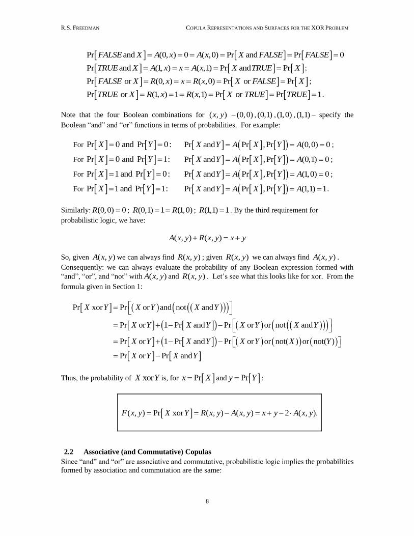
Note that the four Boolean combinations for ( , )x y – (0,0) , (0,1) , (1,0) , (1,1) – specify the
Boolean “and” and “or” functions in terms of probabilities. For example:
For Pr 0 and Pr 0:X Y Pr and Pr ,Pr (0,0) 0X Y A X Y A ;
For Pr 0 and Pr 1:X Y Pr and Pr ,Pr (0,1) 0X Y A X Y A ;
For Pr 1 and Pr 0:X Y Pr and Pr ,Pr (1,0) 0X Y A X Y A ;
For Pr 1 and Pr 1:X Y Pr and Pr ,Pr (1,1) 1X Y A X Y A .
Similarly: (0,0) 0R ; (0,1) 1 (1,0)R R ; (1,1) 1R . By the third requirement for
probabilistic logic, we have:
( , ) ( , )A x y R x y x y
So, given ( , )A x y we can always find ( , )R x y ; given ( , )R x y we can always find ( , )A x y .
Consequently: we can always evaluate the probability of any Boolean expression formed with
“and”, “or”, and “not” with ( , )A x y and ( , )R x y . Let’s see what this looks like for xor. From the
formula given in Section 1:
Pr xor Pr or and not and
Pr or 1 Pr and Pr or or not and
Pr or 1 Pr and Pr or or not( ) or not( )
Pr or Pr and
X Y X Y X Y
X Y X Y X Y X Y
X Y X Y X Y X Y
X Y X Y
Thus, the probability of xorX Y is, for Prx X and Pry Y :
( , ) Pr xor ( , ) ( , ) 2 ( , ).F x y X Y R x y A x y x y A x y
2.2 Associative (and Commutative) Copulas
Since “and” and “or” are associative and commutative, probabilistic logic implies the probabilities
formed by association and commutation are the same:

R.S. FREEDMAN COPULA REPRESENTATIONS AND SURFACES FOR THE XOR PROBLEM
9
Pr and and Pr and andX Y Z X Y Z ;
Pr or or Pr or or X Y Z X Y Z ;
Pr and Pr andX Y Y X ;
Pr or Pr or X Y Y X .
Let andW Y Z and andV X Y . Since the probabilities of association are equal,
Pr and Pr ,Pr Pr ,Pr and Pr , Pr ,PrX W A X W A X Y Z A X A Y Z
Pr and Pr ,Pr Pr and ,Pr Pr ,Pr ,PrV Z A V Z A X Y Z A A X Y Z
So Pr and Pr andX W V Z implies , , , ,A x A y z A A x y z : ( , )A x y is associative.
( , )A x y is also commutative, since ( , ) Pr and Pr and ( , )A x y X Y Y X A y x . Similarly,
( , )R x y is associative and commutative.
It turns out that these properties completely specify a function family. Frank [5] proved
the following result: Let ( , )A x y and ( , )R x y be real-valued functions defined on 1 20 , 1x x
so that 1 2 1 20 ( , ), ( , ) 1A x x R x x . Suppose they are (a) both continuous and associative; (b) are
related by ( , ) ( , )A x y R x y x y ; and (c) satisfy the four conditions:
(0, ) 0 ( ,0)A x A x ; (1, ) ( ,1)A x x A x ;
(0, ) ( ,0)R x x R x ; (1, ) 1 ( ,1)R x R x .
Then the only functions ( , )A x y , ( , )R x y that satisfy (a-c) have the parameterized representations
s 1 2( , ) A ( , )A x y x x where:
For (0, ), 1s s : 1 21 1
s 1 2
1 1A ( , ) log 1
1
x x
s
s sx x
s
when 0s : 0 1 2 1 2A ( , ) min( , )x x x x
when 1s : 1 1 2 1 2A ( , )x x x x
when s : 1 2 1 2A ( , ) max( 1,0)x x x x
Function A ( , )s x y is an example of an Archimedean copula [6]. In probability theory, copula
functions correspond to representations of a joint density of a set of arbitrary random variables in
terms of a joint density of a set of uniformly distributed random variables. In the context of
probabilistic logic, copulas provide a consistent way to extend a set of Boolean (0,1) values to a set
of analog values between 0 and 1. If the Boolean samples (inputs and outputs) are consistent with
probabilistic logic, then the probability of a statement represented as a Boolean function can
represented with operations involving A ( , )s x y and R ( , )s x y . Note the inequalities:

R.S. FREEDMAN COPULA REPRESENTATIONS AND SURFACES FOR THE XOR PROBLEM
10
1 2 1 1 2 0 1 2A ( , ) A ( , ) A ( , )x x x x x x so that 1 2 1 2 1 2A ( , ) A ( , ) A ( , )s ox x x x x x for 0 s .
For the xor representation problem, we have from above that Frank’s parameterization implies:
1 2 1 2 1 2 1 2 1 2( , ) F , : R ( , ) A ( , ) 2 A ( , )s s s sF x y x x x x x x x x x x .
The four conditions (c) imply
F ,0 F 0,s sx x x and F ,1 F 1, 1s sx x x .
Note that for 1 2F ,s x x , the xor inequalities are:
0 1 2 1 1 2 1 2F ( , ) F ( , ) F ( , )x x x x x x so that 0 1 2 1 2 1 2F ( , ) F ( , ) F ( , )sx x x x x x for 0 s .
Figure 2.2 shows three dimensional charts of 0 1 2F ,x x , 1 1 2F ,x x , and 1 2F ,x x : the left sides
of the figure plots 1 2, ,x x z with height 1 2F ,sz x x ; the right side plots the three dimensional
contours (the lines where xor has a constant value). Figure 2.3 shows three dimensional charts for
s=0.01; 0.5; 0.75; 1.25; 2, 20. These formulas are continuous functions defined for all 1 2,x x
between 0 and 1: they also agree with the xor specification at the 4 corner sample points
F 0,0 0 F (1,1); F 0,1 F 1,0 1s s s s . They continuously interpolate xor. Note that 0F and F
both have sharp corners and sharp folds: this implies the gradients (slopes) at those corners and
folds are not continuous.
Note that these copula functions have multiple representations. To see this, recall the Heaviside
unit step function ( )u t which can be defined by: ( ) 1, 0u t t and 0 for 0t . Note that
( ) ( )x x u x x u x
( ) ( )x x u x x u x
( ) ( ) ( ) ( )x y x u y x x u x y y u y x y u x y
min( , ) ( ) ( )x y x u y x y u x y
So, for example, min( , ) ( ) ( ) max( , )x y x y x u x y y u y x x y . This implies
0 1 2 1 2 1 2 1 2F , : max , min ,x x x x x x x x .
Thus, the only representations of xor that is consistent with probabilistic logic, is 1 2F ,s x x :
0 1 2 1 2 1 2 1 2 1 2F , 2 min( , ) max( , ) min( , )x x x x x x x x x x ;
1 1 2 1 2 1 2F , 2x x x x x x ;
1 21 1
1 2 1 2
1 1F , 2 log 1
1
x x
s s
s sx x x x
s
, 0 , 1s s ;
1 2 1 2 1 2F , 2 max( 1,0)x x x x x x 1 2 1 2min( ,1) max( 1,0)x x x x .

R.S. FREEDMAN COPULA REPRESENTATIONS AND SURFACES FOR THE XOR PROBLEM
11
Figure 2.2. Copula solutions to the xor representation problem: s=0; s=1; s=∞.
10.75
0.5
0.25
0
1
0.75
0.5
0.25
0
0.8
0.6
0.4
0.2
x
y
z
10.75
0.50.25
0
1
0.75
0.5
0.25
0
0.8
0.6
0.4
0.2
x
y
z
10.75
0.50.25
0
1
0.75
0.5
0.25
0
1
0.75
0.5
0.25
0
x1
x2
z
xor: F3
10.75
0.50.25
0
1
0.75
0.5
0.25
0
0.8
0.6
0.4
0.2
x
y
z
10.75
0.5
0.25
0
1
0.75
0.5
0.25
0
1
0.75
0.5
0.25
0
x1
x2
z
xor: F0
10.75
0.50.25
0
10.75
0.5
0.25
0
1
0.75
0.5
0.25
0
x1
x2
z
xor: F1
10.75
0.50.25
0
1
0.75
0.5
0.25
0
1
0.75
0.5
0.25
0
x1
x2
z
xor: Finf

R.S. FREEDMAN COPULA REPRESENTATIONS AND SURFACES FOR THE XOR PROBLEM
12
Figure 2.3. Copula solutions to the xor representation problem for various values of s.
10.75
0.50.25
0
1
0.75
0.5
0.25
0
1
0.75
0.5
0.25
0
x1
x2
z
xor: Fs; s=0.5
10.75
0.50.25
0
10.75
0.5
0.25
0
1
0.75
0.5
0.25
0
x1
x2
z
xor: Fs; s=0.75
10.75
0.50.25
0
10.75
0.5
0.25
0
1
0.75
0.5
0.25
0
x1
x2
z
xor: Fs; s=1.25
10.75
0.50.25
0
10.75
0.5
0.25
0
1
0.75
0.5
0.25
0
x1
x2
z
xor: Fs; s=2
10.75
0.50.25
0
10.75
0.5
0.25
0
1
0.75
0.5
0.25
0
x1
x2
z
xor: Fs; s=20
10.75
0.50.25
0
10.75
0.5
0.25
0
1
0.75
0.5
0.25
0
x1
x2
z
xor: Fs; s=0.01

R.S. FREEDMAN COPULA REPRESENTATIONS AND SURFACES FOR THE XOR PROBLEM
13
2.3 Representations of xor with Frank’s Copulas
Let’s review the truth assignments of Figure 1.1 and 2.1 to examine consistency with the
probabilistic inequalities and Frank’s associative copula. The Figure 1.1 assignment is consistent
with the probabilistic logic inequalities:
1 2 1 2Pr and X 0.25 min Pr ,Pr min 0.5,0.5 0.5X X X ;
1 2 1 20.5 max 0.5,0.5 max Pr ,Pr Pr or X 0.75X X X .
Also note that according to Figure 1.1, 1 2Pr Pr 0.5X X and 1 2Pr and X 0.25X . When
we solve for s in A 0.5,0.5 0.25s , we find that s=1 in Frank’s representation. The xor
probability evaluates to 1 1 11 1 2 1 22 2 4
F , ( ) 2 0.5 Pr xor Xx x X .
The Figure 2.1 assignment is also consistent with the probabilistic logic inequalities:
1 2 1 2Pr and X 0.3 min Pr ,Pr min 0.5,0.5 0.5X X X ;
1 2 1 20.5 max 0.5,0.5 max Pr ,Pr Pr or X 0.7X X X .
According to Figure 2.1, 1 2Pr Pr 0.5X X and 1 2Pr and X 0.3X . When we solve for s
in A 0.5,0.5 0.3s , we find that 0.193s in Frank’s representation. The xor probability
evaluates to 1 11 22 2
F 0.5,0.5 ( ) 0.6 0.4 Pr xor Xs X . For another example, consider the
table of Figure 2.4.
Figure 2.4. Another set of 10 random samples from the sample space of Figure 1.1.
The empirical frequencies are 41 10
Pr X ; 72 10
Pr X ; 11 2 10
Pr and XX ; 1 2Pr or X 1X .
The assignment is consistent with the probabilistic logic inequalities:
1 2 1 2Pr and X 0.1 min Pr ,Pr min 0.4,0.7 0.4X X X ;
1 2 1 20.7 max 0.4,0.7 max Pr ,Pr Pr or X 1X X X .
When we solve for s in A 0.4,0.7 0.1s we find that this probability assignment corresponds to
s in Frank’s representation.: A 0.4,0.7 max(0.4 0.7 1,0) 0.1 .
Sample x1 x2 and or xor x1 x2 and or xor Sample
0 1 0 0 1 1 1 1 1 1 0 5
1 0 1 0 1 1 1 0 0 1 1 6
2 1 0 0 1 1 0 1 0 1 1 7
3 0 1 0 1 1 0 1 0 1 1 8
4 0 1 0 1 1 0 1 0 1 1 9

R.S. FREEDMAN COPULA REPRESENTATIONS AND SURFACES FOR THE XOR PROBLEM
14
3 Array Representations of Linear Families
This next two sections review an array notation which helps us account for most functional families
used in machine learning. As with all accounting notations it is easier to see with an example:
these are provided in Figures 3.1-3.4.
First, recall the equation for a line: y a x b . Here, a is the slope and b is the y-intercept.
For two inputs (as in the linear regression examples for xor discussed in Sections 1.2 and 1.3), we
have seen how this generalizes to formulas of the form
11 1 12 2:y w x w x b
Using matrix multiplication (denoted by by mathematicians and MMULT in Excel spreadsheets),
we write this as
1
11 12
2
xw w b
x
y A x b
= MMULT(A,x)+b
Here, x is a column array and A is a row array. We can subsume the constantb further with matrix
multiplication. Create a column array inp by adding an extra row to x and a weight array w by
adding an extra column to A :
1
2:
1
x
x
inp .
Then the output is
1
11 12 13 2 11 1 12 2 13 11 1 12 2 13out : 1
1
x
w w w x w x w x w w x w x w
w inp y .
So inp has an extra row assigned to 1 and w has an additional component where 13w b . Let’s
apply this to the xor problem. Represent each sample x by its own column array inp :
0 0 1 1
(0) : 0 ; (1) : 1 ; (2) : 0 ; (3) : 1
1 1 1 1
inp inp inp inp .
Group them into single array:
0 0 1 1
: 0 1 0 1 .
1 1 1 1
Inputs

R.S. FREEDMAN COPULA REPRESENTATIONS AND SURFACES FOR THE XOR PROBLEM
15
Similarly, group the xor target outputs for all samples in a row array: : 0 1 1 0Targets .
Figure 3.1 shows the original Samples for the xor problem, the array Inputs, and the array Targets.
Figure 3.1. Spreadsheet arrays for the xor representation problem for the linear family.
For the linear family, it can be shown that the weights with the best goodness-of-fit measure (using
the sum of the squares of the errors) is given by the array formula:
=TRANSPOSE( MMULT( MINVERSE( MMULT(INPUTS,TRANSPOSE(INPUTS))), MMULT(INPUTS,TRANSPOSE(TARGETS) ) ) )
This formula uses the spreadsheet array functions MMULT, MINVERSE, and TRANSPOSE. In Figure
3.1, the following formula is entered in the Weights array C17:E17.
=TRANSPOSE( MMULT( MINVERSE( MMULT(C10:F12,TRANSPOSE(C10:F12))), MMULT(C10:F12,TRANSPOSE(C14:F14) ) ) )
Cell E17 shows the weight w3=0.5; the other weights are negligible. Variations of this formula are
used to compute the weights in linear regression.
Let’s introduce a complication by allowing outputs of one formula to be inputs to another. This
feedforward cascade of inputs to outputs to inputs defines “layers” of nested computation. For
example, given inputs 1x and 2x , first compute 1y and 2y and then use these to compute the final
output:
1 1 1
1 11 1 12 2 13
1 1 1
2 11 1 12 2 13
:
:
y w x w x w
y w x w x w
2 2 2
11 1 12 2 13out : w x w x w

R.S. FREEDMAN COPULA REPRESENTATIONS AND SURFACES FOR THE XOR PROBLEM
16
The formulas are easier to see with array notation. From inputs inp to outputs, we introduce the
intermediate arrays y and out1.
The first input is:
1
2:
1
x
x
inp ;
We have as intermediate outputs:
11 1 1 1 1 111 11 12 13 11 1 12 2 13
21 1 1 1 1 1221 22 23 21 1 22 2 23
:
1
xyw w w w x w x w
xyw w w w x w x w
y w inp ;
The second input (also referred to as the “input of the first layer”) is built from the first
intermediate output:
1
2:
1
y
y
out1
The final (second layer) output is then:
1
2 2 2 2 2 2 2 2 2 2
11 12 13 11 12 13 2 11 1 12 2 13out :1
1
y
w w w w w w y w y w y w
yw out1 .
A full evaluation yields:
2 2 2 2
11 1 12 2 13
2 1 1 1 2 1 1 1 2
11 11 1 12 2 13 12 21 1 22 2 23 13
out : w y w y w
w w x w x w w w x w x w w
w out1
This is easier to see on a spreadsheet. Let’s visualize this in Excel: define cell regions inp (the
inputs C10:C12); w1_ and w2_ (two weight regions D10:F11 and H10:J10); and out1_ and out
(the two output regions G10:G12 and K10); and install the array formulas in out1_ and out as
shown:
In mathematical notation, the superscript denotes the weight matrix number, subscript denotes the
row-column coordinates so 1
21w in mathematical notation corresponds to w1_21 in programming
(or spreadsheet) notation. To see examples of computation, populate the weight arrays with some
random values: the results of the formulas using these random weights for out1_and out are:

R.S. FREEDMAN COPULA REPRESENTATIONS AND SURFACES FOR THE XOR PROBLEM
17
The array formulas in the cells are displayed here:
The resultant cascading feedforward network has topology “2-2-1”, corresponding to two
(x1,x2) inputs (2-), two intermediate computed (y1,y2) outputs (-2-), and one final computed output
out (-1 for the last layer). The number of intermediate outputs is also referred to as “the number
of hidden layer units in the neural network.” Note that the initial inputs are not included in the
layer count. The network structure can be viewed by using the “Trace Dependents” spreadsheet
tool; the results are seen here:
Does adding layers change the representational power of the linear family? Lets’s see by
adding layers to this 2-2-1 network.
For the first layer, specify the following arrays for the first set of weights:
1 1 1
11 12 13
1 1 1
21 22 23
w w w
w w w
1 1 1w A b so
11 1
1311 12
11 1
2321 22
;ww w
ww w
1 1A b .
For the second layer, specify the following arrays for the second set of weights:
2 2 2 2 2 2
11 12 13w w w w A b so 2 2 2 2 2
11 12 13;w w w A b
Then 1 1 1
y w inp A x b (first layer computation) 2 2 2 out w out1 A y b (second layer computation).
Consequently, by substituting the outputs for the inputs, we obtain:
2 2 2 2 2 2 2 1 1 1 1out A y b A A x b b A A x A b b
inp w_1 out_1 w_2 out
0 0.1 -0.1 0.2 0.1 -0.4 -0.2 0.3 0.18
1 -0.2 0.3 0.1 0.4
1 1

R.S. FREEDMAN COPULA REPRESENTATIONS AND SURFACES FOR THE XOR PROBLEM
18
Thus, the 2-2-1 network can be represented as a 2-1 (single layer) linear equivalent, with the
weights defined by
2 1 2 1 2 w A A A b b
Consequently,
2 1 2 1 2
11 12 13w w w out w inp inp A b inp A A A b b inp
It does not matter how many layers cascade in linear network family: they are equivalent to a single
layer. The 2-n-1 is same as the 2-1 topology. Applying this rule recursively: a 2-n-m-1 network is
the same as a 2-n-1 topology which is the same as a 2-1 topology. (This result generalizes for any
number of inputs since the number of initial inputs is not specified in the matrix multiplications.)
As before, this is easiest to see on a spreadsheet: see Figure 3.2.
Figure 3.2. Moving from top to bottom: (1) a 2-2-1 network showing output values and weight arrays
A1_ and A2_ (in gray) and b1_ and b2_ (yellow); (2) the formula view of the 2-2-1 network; (3) the
equivalent 2-1 network showing the new A_ (gray) and new b_ (yellow); (4) the formulas of the
equivalent 2-1 network showing the new weight formulas and new output formulas.
4 Array Representations of Nonlinear Families
Here we introduce nonlinearities into the feedforward cascading linear networks described in the
previous section. Let ( )f r denote a real valued function, sometimes specified by :f .
What happens when we evaluate a real-valued function on an array? The simplest solution is to
evaluate the function on every element in the array:
inp w1_ A1_ b1_ out1 w2_ A2_ b2_ out
0 0.1 -0.1 0.2 0.1 -0.4 -0.2 0.3 0.18
1 -0.2 0.3 0.1 0.4
1 1

R.S. FREEDMAN COPULA REPRESENTATIONS AND SURFACES FOR THE XOR PROBLEM
19
1 1
2 2
( )( )
( )
x f xf f
x f x
x
In functional programming, this is called “mapping” a function: applying a function to the
components of the array. This is similar to the situation of multiplying an array by a number: we
just multiply every element in the array by the number:
1 1
2 2
x r xr r
x r x
x
This array multiplication is sometimes called scalar multiplication. For example, for real-valued
function ( ) tanh( )f x x ,
1 1 1
2 2 2
tanh( )tanh
tanh( )
x x xf
x x x
.
In machine learning jargon, these mapping functions are called “activation functions.” We show
some examples in Figure 4.1; [7] has a nice table of activation functions used in neural networks.
Function: Math/Excel Name
( ) tanh( )f t t
=tanh(t) Hyperbolic tangent
( ) 1/ (1 exp( ))f t t
=1/(1+exp(-t)) Sigmoid
( ) ( )f t Id t
=t Identity function
( ) ( )f t t u t
=if(t>0,t,0)
Rectified Linear Unit
(RELU)
Figure 4.1. Some Real-Valued Activation Functions.
Mapping a function is a very special case of applying a general nonlinear function on an array. In
general, a nonlinear function that takes pairs of real numbers and returns pairs of real numbers is
denoted by2 2:g . These functions are sometimes called “vector-valued functions.” An
example of such a function is
1 2 1 21
2 12
tanh( )
/ 1 exp( )
x x x xxg
x xx
It is much easier to study mapping of real-valued activation functions then the more general vector
valued nonlinear functions.

R.S. FREEDMAN COPULA REPRESENTATIONS AND SURFACES FOR THE XOR PROBLEM
20
Let’s see how activation function maps look with the 2-1 family. All we need to do is apply
the real-valued activation function to the linear outputs. Here is a nonlinear output:
11 1 12 2 13out : ( )f w x w x w .
Note that for the identity function ( ) ( )f t Id t t , this nonlinear family reduces to the linear family
since in this case 11 1 12 2 13 11 1 12 2 13out : ( )Id w x w x w w x w x w .
Next, let’s look at the nonlinear 2-2-1 network family. Apply function 1f to the intermediate
linear outputs to obtain:
1 1 1
1 11 1 12 2 13 11
1 11 1 1
21 21 1 22 2 23
f w x w x w yf f
yf w x w x w
1 1y A x b w inp
The second input is built from the first intermediate outputs:
1
2:
1
y
y
out1
The final output is then derived by applying a function 2f to the final linear output:
2 2 2 2
2 2 11 12 13
1
2 2 2 2 2 2
2 11 12 13 2 2 11 1 12 2 13
out :1
1
f f w w w
y
f w w w y f w y w y w
yw out1
A full evaluation yields:
2 2 2 2
2 2 11 1 12 2 13
2 1 1 1 2 1 1 1 2
2 11 1 11 1 12 2 13 12 1 21 1 22 2 23 13
out : f f w y w y w
f w f w x w x w w f w x w x w w
w out1
Note that this nonlinear network output reduces to the linear network output (see the bottom of
page 16 in Section 3) when all activation functions are set to the identity function: 1 2f f Id .
However, in general, the nonlinear 2-2-1 network cannot be simplified.
In analogy to the network topology notation (i.e., “2-2-1”) we introduce a network activation
notation. For example, “inp-f1-f2” means that we use f1 as the activation function of the first layer,
and f2 as the activation function of the second (final output) layer.
Let’s visualize this in Excel. Define cell regions inp (the inputs C10:C12); w1_ and w2_ (two
weight regions D10:F11 and H10:J10); and out1 and out (the two output regions G10:G12 and
K10), as shown:

R.S. FREEDMAN COPULA REPRESENTATIONS AND SURFACES FOR THE XOR PROBLEM
21
This 2-2-1/inp-f1-f2 specification looks very similar to the 2-2-1 network of linear functions we
discussed in Section 3. In our notation, the linear network specified by 2-2-1 is identical to by 2-
2-1/inp-f1-f2 for f1=f2=Id. The network structure can be viewed by using the Trace Dependents
spreadsheet tool; the results are seen in Figure 4.1 showing 2-2-1/inp-tanh-tanh.
Figure 4.1. 2-2-1 topology showing output cell dependency network, random values
for weights, for network 2-2-1/inp-tanh-tanh.
Nonlinear networks of the type where the nonlinearity is created by mapping real-valued activation
functions have “universal approximation capabilities” as described by [8-10]. Essentially this
means that just as we can approximate any real number (like or 2 ) by a fraction or decimal to
any degree of accuracy, so we can approximate any bounded continuous function by a nonlinear
feedforward network with a sufficiently large number of intermediate outputs. This implies that
any bounded continuous function with two inputs can be approximated by a 2-n-1/inp-f1-f2
network with n sufficiently large. Just as the rational numbers are dense on the real line, so are
these nonlinear networks dense in a function space. The goodness-of-fit error decreases as the
number of intermediate (hidden layer) outputs increases. For a 2-n-1 network, theory indicates that
the approximation error decreases inversely proportional to n (i.e., quadrupling the number of
hidden layer outputs should halve the error). Even though many of these theoretical results are not
constructive, there exists powerful time-tested algorithms, such as backpropagation, that yield
approximations that are consistent with theory. Implementations of back propagation are described
in [11-13].
inp w1_ out1 w2_ out
0 0.1 -0.1 0.2 0.099667995 -0.4 -0.2 0.3 0.182089511
1 -0.2 0.3 0.1 0.379948962
1 1
inp w1_ out1 w2_ out
0 0.1 -0.1 0.2 0.099667995 -0.4 -0.2 0.3 0.182089511
1 -0.2 0.3 0.1 0.379948962
1 1
R.S. FREEDMAN COPULA REPRESENTATIONS AND SURFACES FOR THE XOR PROBLEM
22
5 Results of Machine Learning on the Xor Approximation Problem
We showed in Section 1 that there is no linear formula that solves the xor representation or
approximation problem. We showed in Section 3 that by extension, there is no linear feedforward
network that solves the xor representation or approximation problem. However, Section 4
concluded by observing that nonlinear feedforward networks can approximate any bounded
continuous function. In this Section we see how well backpropagation performs on the xor
approximation problem. Note that backpropagation is a search procedure: an iterative form of the
method used in calculus that finds critical points of the weights represented as an error surface.
From a starting point of random weights, it picks an input (from the given set of input samples: also
called the in-sample training set) and computes the corresponding output and slopes (gradients)
with respect to the error surface. It uses the slopes to adjust the weights. After successive steps,
we meander through the error surface over the in-sample data to find a bottom. The goal (or hope)
is that the sequence of steps will get closer and closer to an error minimum.
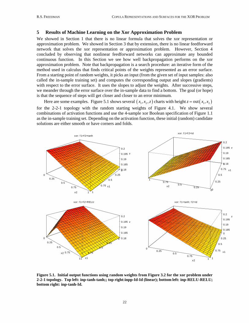
Here are some examples. Figure 5.1 shows several 1 2, ,x x z charts with height 1 2out ,z x x
for the 2-2-1 topology with the random starting weights of Figure 4.1. We show several
combinations of activation functions and use the 4-sample xor Boolean specification of Figure 1.1
as the in-sample training set. Depending on the activation function, these initial (random) candidate
solutions are either smooth or have corners and folds.
Figure 5.1. Initial output functions using random weights from Figure 3.2 for the xor problem under
2-2-1 topology. Top left: inp-tanh-tanh;; top right:inpp-Id-Id (linear); bottom left: inp-RELU-RELU;
bottom right: inp-tanh-Id.
1
0.75
0.5
0.25
0
1
0.75
0.5
0.25
0
0.2
0.195
0.19
0.185
0.18
x1
x2
z
xor: f 1=f 2=tanh
1
0.75
0.5
0.25
0
10.75
0.50.25
0
0.2
0.195
0.19
0.185
0.18
x1
x2
z
xor: f 1=f 2=Id
1
0.75
0.5
0.25
0
1
0.75
0.5
0.25
0
0.2
0.195
0.19
0.185
0.18
x1
x2
z
xor: f 1=f 2=RELU
1
0.75
0.5
0.25
0
10.75
0.50.25
0
0.2
0.195
0.19
0.185
x1
x2
z
xor: f 1=tanh; f 2=Id

R.S. FREEDMAN COPULA REPRESENTATIONS AND SURFACES FOR THE XOR PROBLEM
23
The figures show the results of backpropagation for the 2-2-1 network with different activation
functions. The in-sample training set was the 4-sample Boolean xor specification (Figure 1.1).
Training stopped after a few hundred iterations when the goodness-of-fit error was less than 0.001.
5.1 Xor with tanh-tanh Approximation
Figure 5.2 shows two solutions to the xor approximation problem, corresponding to two separate
runs of backpropagation, for the 2-2-1 inp-tanh-tanh network. The algorithm derived two similar
solutions (each solution corresponds to two different sets of weights); the resultant outputs for in-
sample (the 4 Boolean inputs charted as the four corners in 1 2,x x space) and out-sample (all points
interior to the corners: 1 20 , 1x x ) are shown on the charts below. The charts show the learned
outputs as a 1 2, ,x x z chart with height 1 2out ,z x x together with, for comparison, the optimal
regression solution 1 2out , 0.5x x .
Figure 5.2. Weights and output values for 2-2-1 topology with activation inp-tanh-tanh after machine
learning via backpropagation.
As expected, both outputs correctly interpolate and approximate xor to reasonable accuracy on the
four input training samples: corners 1 2( , )x x (0,0), (0,1), (1,0), (1,1). All other non-corner 1 2( , )x x
points on the graph are out-sample values. The function corresponding to Figure 5.2 looks like it is
learning – in the limit – a non-continuous function that is unity everywhere in 1 20 , 1x x except
at two corner endpoints when it is zero:
1 2 1 2
1 2 1 2
0, 0 or 1; out ,
1, otherwise.
x x x xx x u x x
inp w_1 out_1 w_2 (bias) out Note
0.75 2.320 2.331 -0.850 0.967746 2.68 -2.704 -0.826 0.994616 ???
0.5 1.743 1.747 -2.653 -0.44002 inp-tanh-tanh
1 1
inp w_1 out_1 w_2 out Note
0.75 1.665276 1.665982865 -2.42363 -0.32898 -2.46545 2.490741 -0.71314 0.98685 ???
0.5 2.318576 2.329324919 -0.84434 0.967984 inp-tanh-tanh
1 1
1
0.75
0.50.25
0
1
0.75
0.5
0.25
0
1
0.75
0.5
0.25
0
x1
x2
z
2-1(f 1=Id); 2-2-1(f 1=f 2=tanh)
10.75
0.50.25
0
10.75
0.5
0.25
0
1
0.75
0.5
0.25
0
x1
x2
z
xor: f 1=f 2=tanh

R.S. FREEDMAN COPULA REPRESENTATIONS AND SURFACES FOR THE XOR PROBLEM
24
5.2 Xor with RELU-RELU Approximation
Figure 5.3 shows two solutions for the 2-2-1 inp-RELU-RELU network. As above, the algorithm
derived two solutions corresponding to two different sets of weights; the resultant outputs for in-
sample (the four corners) and out-sample (interior to the corners) are shown on the charts below.
The charts show the learned outputs as a 1 2, ,x x z chart with height 1 2out ,z x x together with,
for comparison, the optimal regression solution 1 2out , 0.5x x .
Figure 5.3. Weights and output values for 2-2-1 topology with activation inp-RELU-RELU after
machine learning via backpropagation.
As expected, both outputs correctly interpolate and approximate xor to reasonable accuracy on the
four input training samples: the corners 1 2( , )x x (0,0), (0,1), (1,0), (1,1). All other non-corner
1 2( , )x x points on the graph are out-sample values. The function corresponding to the first set of
weights (charted in the bottom left of Figure 5.3) looks like Frank’s copula-based continuous
function with s=0. The function corresponding to the second set of weights (charted in the bottom
right of Figure 5.3) also looks like Frank’s copula-based continuous function with s=∞:
0 1 2 1 2 1 2F , 2 min( , )x x x x x x and 1 2 1 2 1 2F , 2 max( 1,0)x x x x x x .
This is a somewhat surprising result. Is this result to consistent with probabilistic logic? If so,
we need to interpret all input and output values as probabilities. So for example, consider the input
values shown in Figure 5.2 where 1 2( , ) (0.75,0.5)x x . The output of machine learning for the first
set of weights, is (0.75,0.5) 0.25F , consistent with 0F . The machine learning output for the
second set of weights is (0.75,0.5) 0.75F , consistent with F . Clearly for these values the
inp w_1 out_1 w_2 out Note
0.75 0.809 -0.809 0.809 1.01125 -1.236 1.64 1 0.250295 F0
0.5 1.220 -1.220 0.000 0.305 inp-RELU-RELU
1 1
10.75
0.50.25
0
1
0.75
0.5
0.25
0
1
0.75
0.5
0.25
0
x1
x2
z
xor (F0) f 1=f 2=RELU
10.75
0.50.25
0
1
0.75
0.5
0.25
0
1
0.75
0.5
0.25
0
x1
x2
z
xor(Finf ) f 1=f 2=RELU

R.S. FREEDMAN COPULA REPRESENTATIONS AND SURFACES FOR THE XOR PROBLEM
25
probabilistic inequality holds: 0 1 2 1 2 1 2( , ) ( , ) ( , )sF x x F x x F x x . Both outputs are consistent with
probabilistic logic and are reasonable approximations to the xor copula representations.
We repeated several experiments using different random starting points and different
topologies. We were surprised to see that the majority of the converging inp-RELU-RELU and
inp-RELU-ID networks converged to 1 2F ,x x ; 0 1 2F ,x x came in second. Figure 5.4 shows
some other sample runs associated with the inp-RELU-RELU xor approximations.
Figure 5.4. Weights and output values for 2-2-1 topology with activation inp-RELU-RELU after
machine learning via backpropagation. Top: weights shown as Cases A-D. Bottom: Charts
corresponding to Cases A-D.
10.75
0.50.25
0
1
0.75
0.5
0.25
0
1
0.75
0.5
0.25
0
x1
x2
z
Case B. F0: f 1=f 2=RELU
1
0.750.5
0.250
1
0.75
0.5
0.25
0
1
0.75
0.5
0.25
0
x1
x2
z
Case A. Finf : f 1=f 2=RELU
10.75
0.50.25
0
1
0.75
0.5
0.25
0
1
0.75
0.5
0.25
0
x1
x2
z
Case C. Finf : f 1=f 2=RELU
10.75
0.50.25
0
1
0.75
0.5
0.25
0
1
0.75
0.5
0.25
0
x1
x2
z
Case D. Finf : f 1=RELU; f 2=Id
inp w_1 out_1 w_2 out Note
0.5 -0.72997 -0.77859375 0.729975 0 -1.36991 -0.97496 1 0.75 Finf
A. 0.75 1.025686 1.025685969 -1.02569 0.256421 inp-RELU-RELU
1 1
inp w_1 out_1 w_2 out Note
0.5 1.424852 -1.33709869 -0.08775 0 1.495776 -1.2846 1 0.25 F0
B. 0.75 0.778454 -0.77845371 0.778454 0.58384 inp-RELU-RELU
1 1
inp w_1 out_1 w_2 out Note
0.5 0.934582 0.934581882 -0.93458 0.233645 -1.07 -1.23175 1 0.75 Finf
C. 0.75 -0.81185 -0.81185454 0.811855 0 inp-RELU-RELU
1 1
inp w_1 out_1 w_2 out Note
0.5 0.765382 0.765416316 2.34E-05 0.956777 1.306379 -1.68037 6.83E-05 0.751068 Finf
D. 0.75 1.187765 1.187746159 -1.18779 0.296907 inp-RELU-Id
1 1

R.S. FREEDMAN COPULA REPRESENTATIONS AND SURFACES FOR THE XOR PROBLEM
26
6 Error Tabulation and Error Surfaces
Understanding convergence requires an understanding of the error surface. Recall the 2-1 linear
network (used in linear regression) with output
11 1 12 2 13out : w x w x w
The linear regression problem is to find values for the three weights so that the errors are as small
as possible. Recall that we are able to visualize the output by plotting 1 2, ,x x z with height
1 2out ,z x x . For the output chart there are 2 degrees of freedom (dimensions) for the inputs:
this implies that visualizing the problem requires charting a 2-dimensional surface in 3-dimensional
space.
Using the 4-sample Boolean specification as the training set (Figure 1.1), the equation for the
goodness-of-fit error (using sum of squares) is:
2 2 2 2
2 2 2 2
3 1 2 3 1 3 2 3
err: out 0,0 0 out 0,1 1 out 1,0 1 out 1,1 0
1 1w w w w w w w w
Can we do the same thing with by plotting this goodness-of-fit error function? There are 3 degrees
of freedom for the weights 1 2 3, ,w w w : visualizing the problem requires plotting 1 2 3, , ,w w w z
with height 1 2 3err , ,z w w w . This requires charting a 3-dimensional error surface in 4-
dimensional space. Unfortunately our visual perception is limited to three dimensions.
The situation is more complex for nonlinear network topologies. The 2-2-1 nonlinear output
is (Section 4)
2 1 1 1 2 1 1 1 2
2 11 1 11 1 12 2 13 12 1 21 1 22 2 23 13out : f w f w x w x w w f w x w x w w
For the 4-sample Boolean training set, the equation for the goodness-of-fit is:
22 2 1 2 1
2 13 11 1 13 12 1 23
22 2 1 1 1 2 1 1 1
2 13 11 1 11 12 13 12 1 21 22 23
22 2 1 1 2 1 1
2 13 11 1 11 13 12 1 21 23
22 2 1 1 2 1 1
2 13 11 1 12 13 12 1 22 23
err:= ( ) ( )
( ) ( )
( ) ( ) 1
( ) ( ) 1
f w w f w w f w
f w w f w w w w f w w w
f w w f w w w f w w
f w w f w w w f w w
Visualizing the problem requires plotting 1 1 1 1 1 1 2 2 2
11 12 13 21 22 23 11 12 13, , , , , , , , ,w w w w w w w w w z with height
1 1 1 1 1 1 2 2 2
11 12 13 21 22 23 11 12 13err , , , , , , , ,z w w w w w w w w w . For the goodness-of-fit plot there are 9 degrees of
freedom (dimensions) for the weights: visualizing the problem requires charting a 9-dimensional
error surface in 10-dimensional space. One solution is to restrict ourselves to 2-dimensional error
surface slices. For example, let’s simplify the problem to 2 degrees of freedom by assigning the

R.S. FREEDMAN COPULA REPRESENTATIONS AND SURFACES FOR THE XOR PROBLEM
27
values tabulated in Figure 3.2 to all weights except for 1
11w and 1
12w . This error surface formula –
called the 1 1
11 12w w projection – is:
2
11 12 2 1 1
21 1
2 1 11 12 1
21
2 1 11 1
21
2 1 12 1
err( , ):= 0.3 0.4 (0.2) 0.2 (0.1)
0.3 0.4 ( 0.2) 0.2 (0.2)
0.3 0.4 ( 0.2) 0.2 ( 0.1) 1
0.3 0.4 ( 0.2) 0.2 (0.4) 1
w w f f f
f f w w f
f f w f
f f w f
There is nothing special about1
11w and 1
12w . We could have selected any two weights to get a 2-
dimensional projection of the 9-dimensional surface. These are straightforward to configure and
plot with any computer algebra system.
The following pages show several three-dimensional charts for different projections of the 2-
dimensional error surface for the xor problem. For the 2-2-1 topology, there are
936
2
projections. The horizontal (xy) plane shows the values in the two-dimensional weight-space; the
vertical (z axis) shows the value of the error surface (sums of squares of the errors over all four
samples). We also show these values represented as a three-dimensional contour display. Our
parameters are the different output functions:
Id( ) ; tanh( ); RELU( )t t t t
The first figure shows the case where 1 2( ) ( )f z f z z : this is the same case as the linear
network family in Section 3. The equation for the error surface using sum of squared errors is:
2
11 12 11 12 12 2
2 2
11 12
err( , ):= 0.18 0.4 0.4 0.04 0.06 0.2
0.4 0.76 0.4 0.86 0.04
w w w w w x
w w
As expected, the error surface is a paraboloid bowl with a single global minimum (a unique
solution) and no valleys or hidden peaks. The other nonlinear functions show the complexity of
the error surfaces.
Corners and folds present problems for gradient search methods: these shapes induce non-
continuous slopes. Moreover, nonlinear surfaces are might lead candidate solutions to get suck in
local valleys or on non-optimal local peaks or “saddle points.” We can see examples of these with
the error surface charts in Figures 6.1-6.7.

R.S. FREEDMAN COPULA REPRESENTATIONS AND SURFACES FOR THE XOR PROBLEM
28
FIGURE 6.1. Identity function. Linear Family. For 2-2-1: inp-Id-Id.
52.5
0-2.5
-5
52.5
0-2.5
-5
25
20
15
10
5
x
y
z
52.50-2.5-5 52.50-2.5-5
30
25
20
15
10
5
wxwy
z
SmSqErs: w1_11 x w1_12: f 1=f 2=ID
52.5
0-2.5
-5
5
2.5
0
-2.5
-5
17.5
15
12.5
10
7.5
5
2.5
wx
wy
z
SmSqErs: w2_11 x w2_12: f 1=f 2=ID
52.5
0-2.5
-5
5
2.5
0
-2.5
-5
15
12.5
10
7.5
5
2.5
x
y
z
52.5
0-2.5
-5
5
2.5
0
-2.5
-5
20
17.5
15
12.5
10
7.5
5
2.5
wx
wy
z
SmSqErs: w1_11 x w2_12: f 1=f 2=ID
52.5
0-2.5
-5
5
2.5
0
-2.5
-5
17.5
15
12.5
10
7.5
5
2.5
x
y
z

R.S. FREEDMAN COPULA REPRESENTATIONS AND SURFACES FOR THE XOR PROBLEM
29
FIGURE 6.2. RELU function. RELU Family. For 2-2-1: inp-RELU-RELU:
5
2.5
0
-2.5
-5
5
2.5
0
-2.5
-5
2
1.8
1.6
1.4
x
y
z
52.5
0-2.5
-5
52.5
0-2.5
-5
10
7.5
5
2.5
wx
wy
z
SmSqErs: w2_11 x w2_12: f 1=f 2=RELU
5
2.5
0
-2.5
-5
5
2.5
0
-2.5
-5
10
7.5
5
2.5
x
y
z
5
2.5
0
-2.5
-5
52.5
0-2.5
-5
4
3.5
3
2.5
2
1.5
1
wx
wy
z
SmSqErs: w1_11 x w2_12: f 1=f 2=RELU
5
2.5
0
-2.5
-5
5 2.5 0 -2.5 -5
4
3.5
3
2.5
2
1.5
1
x
y
z
5
2.5
0
-2.5
-5
5
2.5
0
-2.5
-5
2
1.8
1.6
1.4
wx
wy
z
SmSqErs: w1_11 x w1_12: f 1=f 2=RELU

R.S. FREEDMAN COPULA REPRESENTATIONS AND SURFACES FOR THE XOR PROBLEM
30
FIGURE 6.3. Ridge Functions. For 2-2-1:. Surface w1_11 x w1_12.
52.5
0-2.5
-5
5
2.5
0
-2.5
-5
2.5
2.25
2
1.75
1.5
1.25
1
x
y
z
5
2.5
0
-2.5
-5
5
2.5
0
-2.5
-5
2.5
2.25
2
1.75
1.51.25
10.75
w11
w12
z
Sum Squared Errors: f 1=tanh;f 2=Id
52.50-2.5-5
52.5
0-2.5
-5
30
25
20
15
10
5
w11
w12
z
Sum Squared Errors: f 1=RELU;f 2=Id
52.5
0-2.5
-5
52.5
0-2.5
-5
25
20
15
10
5
x
y
z
52.5
0-2.5
-5
5
2.5
0
-2.5
-5
2.75
2.5
2.25
2
1.75
1.5
w1
w2
z
Sum Squared Errors: f 1=sigm;f 2=Id
52.5
0-2.5
-5
5
2.5
0
-2.5
-5
2.75
2.5
2.25
2
1.75
1.5
x
y
z

R.S. FREEDMAN COPULA REPRESENTATIONS AND SURFACES FOR THE XOR PROBLEM
31
FIGURE 6.4. Same activation function for both layers: f1=f2. Surface w1_11 x w1_12.
5
2.5
0
-2.5
-5
5
2.5
0
-2.5
-5
2.5
2.25
2
1.75
1.5
1.25
1
x
y
z
52.5
0-2.5
-5
5
2.5
0
-2.5
-5
2.5
2.25
2
1.75
1.5
1.25
1
0.75
w11
w12
z
Sum Squared Errors: f 1=tanh;f 2=tanh
5
2.5
0-2.5
-5
5
2.5
0
-2.5
-5
2
1.8
1.6
1.4
w11
w12
z
Sum Squared Errors: f 1=f 2=RELU
5
2.5
0
-2.5
-5
5
2.5
0
-2.5
-5
2
1.8
1.6
1.4
x
y
z
5
2.5
0
-2.5
-5
5
2.5
0
-2.5
-5
1.05
1.025
1
0.975
w1
w2
z
Sum Squared Errors: f 1=sigm;f 2=sigm
52.5
0
-2.5
-5
5
2.5
0
-2.5
-5
1.04
1.02
1
0.98
0.96
x
y z

R.S. FREEDMAN COPULA REPRESENTATIONS AND SURFACES FOR THE XOR PROBLEM
32
FIGURE 6.5. Identity function for first layer: f1=Id. Surface w1_11 x w1_12.
52.5
0-2.5-5
5
2.5
0
-2.5
-5
7.5
6.25
5
3.75
2.5
x
y
z
52.5
0-2.5
-5
5
2.5
0
-2.5
-5
7.5
6.25
5
3.75
2.5
1.25
w11
w12
z
Sum Squared Errors: f 1=Id;f 2=tanh
52.50
-2.5-5
52.50-2.5-5
20
17.5
15
12.5
10
7.5
5
2.5
w11
w12
z
Sum Squared Errors: f 1=Id;f 2=RELU
5
2.5
0
-2.5
-5
52.5
0-2.5
-5
17.5
15
12.5
10
7.5
5
2.5
x
y
z
5
2.5
0
-2.5-5 5
2.50
-2.5
-5
1.75
1.625
1.5
1.375
1.25
1.125
w1w2
z
Sum Squared Errors: f 1=Id;f 2=sigm
52.5
0-2.5
-5
5
2.5
0
-2.5
-5
1.625
1.5
1.375
1.25
1.125
x
y
z

R.S. FREEDMAN COPULA REPRESENTATIONS AND SURFACES FOR THE XOR PROBLEM
33
FIGURE 6.6. Same activation function for both layers: f1=f2. Surface w1_11 x w1_21.
52.5
0-2.5
-5
5
2.5
0
-2.5
-5
17.5
15
12.5
10
7.5
5
2.5
w1
w2
z
Sum Squared Errors: f 1=f 2=z
52.5
0-2.5
-5
52.5
0
-2.5
-5
15
12.5
10
7.5
5
2.5
x
y
z
52.5
0-2.5
-5
52.5
0
-2.5
-5
2.25
2
1.75
1.5
1.25
w1
w2
z
Sum Squared Errors: f 1=f 2=tanh
5
2.50
-2.5-5
5
2.5
0
-2.5
-5
2.25
2
1.75
1.5
1.25
x
y
z
5
2.5
0
-2.5
-5
5 2.5 0 -2.5-5
1.7
1.6
1.5
1.4
1.3
wx
wy
z
SmSqErs: w1_11 x w1_21: f 1=f 2=RELU
5
2.5
0
-2.5
-5
5 2.5 0 -2.5-5
1.7
1.6
1.5
1.4
1.3
x
y
z

R.S. FREEDMAN COPULA REPRESENTATIONS AND SURFACES FOR THE XOR PROBLEM
34
FIGURE 6.7. Same activation function for both layers: f1=f2. Surface w1_11 x w2_12.
5
2.5
0
-2.5
-5
5
2.5
0
-2.5
-5
4.543.532.521.5
x
y
z
5
2.5
0
-2.5
-5
52.5
0-2.5
-5
20
17.5
15
12.5
10
7.5
5
2.5
w1
w2
z
Sum Squared Errors: f 1=f 2=Id
52.5
0-2.5
-5
5
2.5
0
-2.5
-5
17.5
15
12.5
10
7.5
5
2.5
x
y
z
5
2.5
0
-2.5
-5
52.5
0-2.5
-5
4.5
4
3.5
3
2.5
2
1.5
w1
w2
z
Sum Squared Errors: f 1=f 2=tanh
52.5
0-2.5
-5
5
2.5
0
-2.5
-5
4
3.5
3
2.5
2
1.5
1
wx
wy
z
SmSqErs: w1_11 x w2_12: f 1=f 2=RELU
52.5
0-2.5
-5
5
2.5
0
-2.5
-5
43.532.521.51
x
yz

R.S. FREEDMAN COPULA REPRESENTATIONS AND SURFACES FOR THE XOR PROBLEM
35
7. Discussion The 2-2-1 xor approximation problem using 4 Boolean inputs as the training set should be simple
enough to completely analyze. Part of our motivation was to try to understand why the simple 2-
2-1 inp-RELU-RELU networks trained to solve the xor representation problem were able to
generalize its results to copula-based xor representations on an out-sample data set of real values
between zero and one. Comparing the outputs of a machine learning experiment with values not
seen in the training set is called cross-validation. In the following, we examine the copula
representations in the context of selecting in-sample and out-sample data for cross-validation.
7.1 From Boolean Values to Analog Values
In Section 2, we have seen that, in the context of probabilistic logic, copulas provide a consistent
way to extend a set of Boolean values to a set of analog values for both inputs and outputs. If a
logical statement can be represented in terms of “and”, “or,” and “not”, then the probability of the
statement can be represented in terms of copulas ( , )sA x y and ( , )sR x y .
The charts shown in Section 5 showed the 2-2-1 networks trained on 4 Boolean inputs: the
corners 1 2( , )x x (0,0), (0,1), (1,0), (1,1). All other non-corner 1 2( , )x x points on the charts are out-
sample values. Comparing the outputs of a machine learning experiment with values not seen in
the training set is called cross-validation. Let’s examine how the copula representations helps in
selecting in-sample and out-sample data for cross-validation. Let 1X and 2X be statements: logical
sentences that are either TRUE (1) or FALSE (0). Let 1 1Prx X and 2 2Prx X . The
plausibility for xor, 1 2 1 2, Pr xor F x x X X , can be presented in the following ways:
Each specification specifies a training set for machine learning or for cross-validation. For
example, the 2-2-1 networks in Section 5 were all trained with the 4-sample Boolean Specification.
What about cross-validation? We showed that many runs of the inp-RELU-RELU network
converged to the copula-based representations 0F or F , and the inp-tanh-tanh network converged
to another function not consistent with probabilistic logic. This shows that one in-sample
specification can result in many valid trained networks with very different characteristics.
Boolean specification:
1,0 0,1 1
0,0 1,1 0
F F
F F
Analog specification:
1, ,1 1
0, ,0
F x F x x
F x F x x
Copula specification:
1 2
0 1 2 1 2 1 2
1 1
1 2 1 2
1 2
1 1 2 1 2 1 2
1 2 1 2 1 2
F , 2 min( , )
1 1F , 2 log 1
1F ,
F , 2
F , 2 max( 1,0)
x x
s s
x x x x x x
s sx x x x
sx x
x x x x x x
x x x x x x

R.S. FREEDMAN COPULA REPRESENTATIONS AND SURFACES FOR THE XOR PROBLEM
36
Note that the xor copula representations for 0F and F have the following RELU
representations:
0 1 2 1 2 1 2 1 2 2 1F , 2 min( , ) RELU RELU RELUx x x x x x x x x x
1 2 1 2 1 2 1 2 1 2F , 2 max( 1,0) RELU RELU( ) 2 RELU( 1)x x x x x x x x x x
These representations are consistent with the 2-2-1 approximations where (see Section 4):
2 1 1 1 2 1 1 1 2
11 11 1 12 2 13 12 21 1 22 2 23 13out RELU RELU RELUw w x w x w w w x w x w w
These copula-based representations for 0F and F are shown in Figure 7.1.
Figure 7.1. Weights and output values for 2-2-1 topology with activation inp-RELU-RELU for exact
network representations for F0 and F∞ , together with linear regression. Compare Figures 5.3 and 5.4.
1
0.75
0.50.25
0
1
0.75
0.5
0.25
0
1
0.75
0.5
0.25
0
x1
x2
z
Finf R: RELU Exact
10.75
0.50.25
0
10.75
0.5
0.25
0
1
0.75
0.5
0.25
0
x1
x2
z
F0R: RELU Exact

R.S. FREEDMAN COPULA REPRESENTATIONS AND SURFACES FOR THE XOR PROBLEM
37
Perhaps for Boolean functions based on logical operations (and thereby consistent with
probabilistic logic), RELU is a better choice for activation functions. On the other hand, we were
unable to show an inp-RELU-RELU network that converged to the copula representation 1F .
Other networks such as inp-tanh-tanh learned the xor function for Boolean in-sample data but
were unable to generalize to other real-valued xor representations. Of course, adding more records
to the in-sample training set, increasing the number of inputs from two to three or more, and
increasing the number of intermediate outputs (hidden layers), improves the approximation. But
what is wrong with fixing the topology or activation function on a simpler implementation that
allows less computational work, more accuracy, and faster convergence? Is there an “activation
function bias” as well as data sample bias (for selecting both in-sample and out-sample data)? In
this sense, we somewhat disagree with Hornick’s observation [8] that
…it’s not the specific choice of the activation function, but rather the multilayer
feedforward architecture itself which gives neural networks the potential of being universal
learning machines.
Figure 7.2 shows an example of a cross-validation out-sample data set with a Boolean
specification. Note that we identified three possible “acceptable” outputs (all shaded)
corresponding to s=0, s=1, and s=∞.
Figure 7.2. Boolean in-sample (4 records) and copula out-sample values (5 records) consistent with
probabilistic logic (s=0, 1,∞).
Again, we interpret numbers between zero and one as informal subjective probabilities. Can they
be interpreted as actual probabilities? If the input and output probabilities are consistent with
probabilistic logic, then it may be that the output corresponds to a copula representation of a
Boolean formula.
Figure 7.3 shows four different in-sample training sets based on the above specifications. One
specification each for Boolean, analog, copula; the fourth combines all three. Note that the analog
and copula training sets are samples of an otherwise infinite set of values. For the combined set,
only one input sample (0.5, 0.5, 0.5) corresponds to a copula specification (s=1). More in-sample
data generally provides more opportunity for learning.

R.S. FREEDMAN COPULA REPRESENTATIONS AND SURFACES FOR THE XOR PROBLEM
38
Figure 7.3. Boolean, Analog, Copula, and All (combined) in-sample training data consistent with
probabilistic logic (s=1).
7.2 Changing Topology: More Intermediate Outputs
In one experiment we doubled the intermediate outputs of the 2-2-1 network to see if the 2-4-1
network with inp-RELU-RELU can learn the s=1 copula. We used the “All” in-sample data set
shown in Figure 7.2. The results, together with the 1 1
11 12w w error surface projection (around the
minimum) are shown in Figure 7.4: inp-RELU-RELU with 2-4-1 topology (with the “All” sample
training set of Figure 7.3) can learn the s=1 representation. Figure 7.5 shows some results of the
2-4-1 network with inp-tanh-tanh with the “All” in-sample set for s=0 and s=1. The charts show
that the results are approximating the s=0 and s=1 copulas. There were mixed results concerning
the consistency with the probabilistic logic inequalities.
Figure 7.4. Results of the 2-4-1 network with inp-RELU-RELU with the “All” 9-sample training set .
10.75
0.50.25
0
1
0.75
0.5
0.25
0
1
0.75
0.5
0.25
0
x1
x2
z
2-4-1:xor(9;s=1): f 1=f 2=RELU
52.5
0-2.5
-5
5
2.5
0
-2.5
-5
3
2.5
2
1.5
1
0.5
wx
wy
z
SmSqErs:2-4-1:xor(9;s=1) w1_11 x w1_12: f 1=f 2=RELU
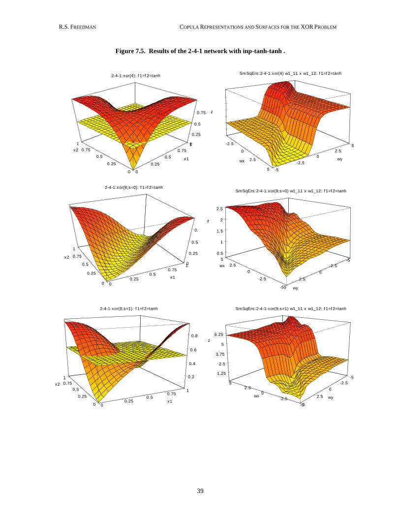
R.S. FREEDMAN COPULA REPRESENTATIONS AND SURFACES FOR THE XOR PROBLEM
39
Figure 7.5. Results of the 2-4-1 network with inp-tanh-tanh .
5
2.5
0
-2.5
-5
5
2.5
0
-2.5
-5
3.5
3
2.5
2
1.5
1
0.5
wx wy
z
SmSqErs:2-4-1:xor(4) w1_11 x w1_12: f 1=f 2=tanh
1
0.75
0.5
0.25
0
1
0.75
0.5
0.25
0
0.75
0.5
0.25
0
x1
x2
z
2-4-1:xor(4): f 1=f 2=tanh
10.75
0.50.25
0
1
0.75
0.5
0.25
0
0.75
0.5
0.25
0
x1
x2
z
2-4-1:xor(9;s=0): f 1=f 2=tanh
5
2.5
0
-2.5
-55
2.5
0
-2.5
-5
2.5
2
1.5
1
0.5
wx
wy
z
SmSqErs:2-4-1:xor(9;s=0) w1_11 x w1_12: f 1=f 2=tanh
10.75
0.50.25
0
1
0.75
0.5
0.25
0
0.8
0.6
0.4
0.2
x1
x2
z
2-4-1:xor(9;s=1): f 1=f 2=tanh
52.5
0
-2.5
-55
2.5
0
-2.5
-5
6.25
5
3.75
2.5
1.25
wx wy
z
SmSqErs:2-4-1:xor(9;s=1) w1_11 x w1_12: f 1=f 2=tanh

R.S. FREEDMAN COPULA REPRESENTATIONS AND SURFACES FOR THE XOR PROBLEM
40
7.3 Changing Topology: More Hidden Layers
We observe that the more weights, the more complex the error surface in terms of folds and corners.
In the last experiment we increased the number of layers. We kept the number of weights fixed. It
is an exercise in accounting to verify that a 2-n-1 network has 4 1n weights; a 2-p-q-1 network
has 3 2 1p q p q weights. Thus the 2-9-1 network (inp-tanh-tanh) and the 2-4-4-1 (inp-
tanh-tanh-tanh) network have the same number of weights (37). We trained both networks on the
4-sample Boolean specification. Given similar in-sample error performance on the in-sample data,
both networks converged to 1 2u x x – the function observed in Section 5.1. Neither network
was consistent with probabilistic logic. The 2-4-4-1 network converged in fewer iterations (having
same goodness-of-fit error of less than 0.001) than the 2-9-1 network. Both networks are posted at
[14].
7.4 Lessons for larger networks?
We do not fully understand why the same 2-2-1 network trained with the same xor Boolean
specification learns (when it converges) either 0F or F . We did not see any other Fs besides the
cases for 0s or s , even though by heuristic grounds we expected to see 1F in some of the
training examples. Even though the error surface projections show the dynamics and problems
associated with gradient search, the only conclusion we could make was that if the search starts
from an unlucky point then the search will get stuck on a plateau.
The only other possibility could be related to the random sampling used in data selection.
Selecting records of Boolean inputs corresponding to truth assignments could bias the underlying
probabilistic logic statement probabilities. Would that be enough to influence the bifurcating xor
convergence mechanism?
In any case: we can always evaluate a probability (consistent with probabilistic logic) of any
Boolean expression formed with “and”, “or”, and “not” with ( , )A x y and ( , )R x y . Since ( , )A x y
and ( , )R x y are associative, this statement is still true for Boolean expressions of any number of
inputs. Nonlinear networks with enough layers are universal approximators; they will converge to
a function – even though (as we have seen with xor) the approximated function might not be the
function that one wants.

R.S. FREEDMAN COPULA REPRESENTATIONS AND SURFACES FOR THE XOR PROBLEM
41
8. References
[1] Wikipedia contributors. (2017, June 9). Boolean Logic. In Wikipedia, The Free Encyclopedia.
URL: https://en.wikipedia.org/wiki/Boolean_logic .
[2] Elizondo, D. (2006) “The linear separability problem: Some testing methods.” IEEE
Transactions on Neural Networks 17.2: 330-344.
[3] Nilsson, N. J. (1986). Probabilistic logic. Artificial Intelligence, 28(1): 71-87.
[4] Guggenheimer, H., & Freedman, R. (1987). Foundations of probabilistic logic. Proceedings
of the 10th International Joint conference on Artificial Intelligence (IJCAI). Vol. 2: 939-941.
Morgan Kaufmann Publishers.
[5] Frank, M. (1979). On the simultaneous associativity of ( , )F x y and ( , )x y F x y .
Aequationes mathematicae, 19(1): 194-226.
[6] Klement, E., Mesiar, R., & Pap, E. (2002). Invariant copulas. Kybernetika, 38(3): 275-286.
[7] Wikipedia contributors. (2019, February 22). Activation function. In Wikipedia, The Free
Encyclopedia. URL: https://en.wikipedia.org/wiki/Activation_function .
[8] Hornik, K. (1991). Approximation capabilities of multilayer feedforward networks. Neural
Networks 4.2: 251-257.
[9] Kůrková, V. (1992). Kolmogorov's theorem and multilayer neural networks. Neural Networks
5.3: 501-506.
[10] Sonoda, S, & Murata, N. (2017) Neural network with unbounded activation functions is
universal approximator. Applied and Computational Harmonic Analysis 43.2: 233-268.
[11] Pao, Y-H (1989). Adaptive Pattern Recognition and Neural Networks. Addison Wesley.
[12] LeCun, Y., Bottou, L., Orr, G., & Müller, K. (2012). Efficient backprop. In Neural Networks:
Tricks of the Trade, Vol. 7700, Lecture Notes in Computer Science: 9-48. Springer.
[13] Freedman, R. Visual backpropagation (2019). arXiv:1906.04011 [cs.LG] .
[14] Visual Backpropagation Examples. URL: https://www.inductive.com/visualbackprop .