copyright © 2009 cengage learning chapter 13 inference about comparing two populations

Copyright © 2009 Cengage Learning

Chapter 13

Inference About ComparingTwo Populations


Comparing Two PopulationsPreviously we looked at techniques to estimate and test parameters for one population:

Population Mean µ Population Proportion p

We will still consider these parameters when we are looking at two populations, however our interest will now be:

The difference between two means. The ratio of two variances. The difference between two

proportions.


Difference between Two MeansIn order to test and estimate the difference between two population means, we draw random samples from each of two populations. Initially, we will consider independent samples, that is, samples that are completely unrelated to one another.

(Likewise, we consider for Population 2)

Sample, size: n1

Population 1

Parameters: Statistics:


Difference between Two Means

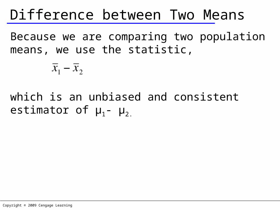
Because we are comparing two population means, we use the statistic,

which is an unbiased and consistent estimator of µ1- µ2.


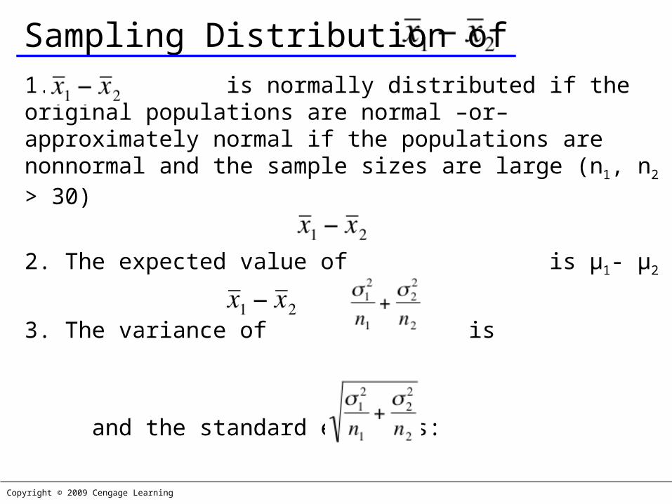
Sampling Distribution of 1. is normally distributed if the original populations are normal –or– approximately normal if the populations are nonnormal and the sample sizes are large (n1, n2 > 30)

2. The expected value of is µ1- µ2

3. The variance of is

and the standard error is:


Making Inferences About μ1-μ2

Since is normally distributed if the original populations are normal –or– approximately normal if the populations are nonnormal and the sample sizes are large, then:

is a standard normal (or approximately normal) random variable.

We could use this to build the test statistic and the confidence interval estimator for µ1 - µ2.


Making Inferences About μ1-μ2

…except that, in practice, the z statistic is rarely used since the population variances are unknown.

Instead we use a t-statistic. We consider two cases for the unknown population variances: when we believe they are equal and conversely when they are not equal.

More about this later…

??


Test Statistic for μ1-μ2 (equal variances) Calculate – the pooled variance

estimator as…

…and use it here:

degrees of freedom


CI Estimator for μ1-μ2 (equal variances) The confidence interval estimator for μ1-

μ2 when the

population variances are equal is given by:

degrees of freedompooled variance estimator


Test Statistic for μ1-μ2 (unequal

variances) The test statistic for μ1-μ2 when the

population variances are unequal is given by:

Likewise, the confidence interval estimator is:

degrees of freedom


Which test to use?

Which test statistic do we use? Equal variance or unequal variance?Whenever there is insufficient evidence that the variances are unequal, it is preferable to perform the

equal variances t-test.This is so, because for any two given samples:The number of degrees of freedom for the equal variances case

The number of degrees of freedom for the unequal variances case

≥

Larger numbers of degrees of freedom have the same effect as having larger

sample sizes

≥


Testing the Population Variances


H0: σ12 / σ2

2 = 1

H1: σ12 / σ2

2 ≠ 1

Test statistic: s12 / s2

2, which is F-distributed with degrees of freedom ν1 = n1– 1 and ν2 = n2 −2.

The required condition is the same as that for the t-test of µ1 - µ2 , which is both populations are normally distributed.



This is a two-tail test so that the rejection region is

or

21 ,,2/FF ννα>

21 ,,2/1FF ννα−<


Example 13.1Millions of investors buy mutual funds choosing from thousands of possibilities.

Some funds can be purchased directly from banks or other financial institutions while others must be purchased through brokers, who charge a fee for this service.

This raises the question, can investors do better by buying mutual funds directly than by purchasing mutual funds through brokers.


Example 13.1To help answer this question a group of researchers randomly sampled the annual returns from mutual funds that can be acquired directly and mutual funds that are bought through brokers and recorded the net annual returns, which are the returns on investment after deducting all relevant fees. Xm13-01

Can we conclude at the 5% significance level that directly-purchased mutual funds outperform mutual funds bought through brokers?


Example 13.1

To answer the question we need to compare the population of returns from direct and the returns from broker- bought mutual funds.

The data are obviously interval (we've recorded real numbers).

This problem objective - data type combination tells us that the parameter to be tested is the difference between two means µ1- µ2.

IDENTIFY


Example 13.1The hypothesis to be tested is that the mean net annual return from directly-purchased mutual funds (µ1) is larger than the mean of broker-purchased funds (µ2). Hence the alternative hypothesis is

H1: µ1- µ2 > 0

and H0: µ1- µ2 = 0

To decide which of the t-tests of µ1 - µ2 to apply we conduct the F-test of σ1

2/ σ22 .

IDENTIFY


Example 13.1From the data we calculated the following statistics.

s12 = 37.49 and s2

2 = 43.34

Test statistic: F = 37.49/43.34 = 0.86

Rejection region:

or

IDENTIFY

60.1FFFF 50,50,025.49,49,025.,,2/ 21=≈=> ννα

63.60.1/1F/1F/1FFF 50,50,025.49,49,025.49,49,975.,,2/1 21==≈==< ννα−


Example 13.1

Click Data, Data Analysis, and F-Test Two Sample for Variances

IDENTIFY


Example 13.1

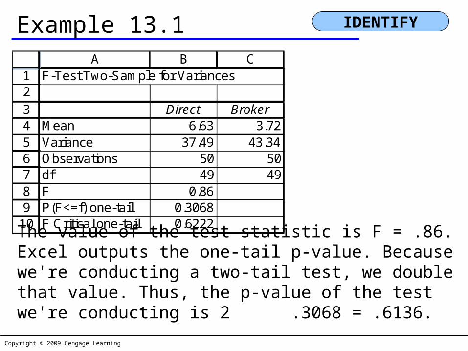
The value of the test statistic is F = .86. Excel outputs the one-tail p-value. Because we're conducting a two-tail test, we double that value. Thus, the p-value of the test we're conducting is 2 .3068 = .6136.

IDENTIFY

123456789

10

A B CF-Test Two-Sample for Variances

Direct BrokerMean 6.63 3.72Variance 37.49 43.34Observations 50 50df 49 49F 0.86P(F<=f) one-tail 0.3068F Critical one-tail 0.6222

×


Example 13.1There is not enough evidence to infer that the population variances differ. It follows that we must apply the equal-variances t-test of µ1- µ2

IDENTIFY

Copyright © 2009 Cengage Learning 12.22

Example 13.1For manual calculations click

Example 13.1 Manual Calculations

For Excel skip to next slide.

COMPUTE


Example 13.1

Click Data, Data Analysis, t-Test: Two-Sample Assuming Equal Variances

COMPUTE


Example 13.1 COMPUTE

12

3456789

1011121314

A B Ct-Test: Two-Sample Assuming Equal Variances

Direct BrokerMean 6.63 3.72Variance 37.49 43.34Observations 50 50Pooled Variance 40.41Hypothesized Mean Difference 0df 98t Stat 2.29P(T<=t) one-tail 0.0122t Critical one-tail 1.6606P(T<=t) two-tail 0.0243t Critical two-tail 1.9845


Example 13.1

The value of the test statistic is 2.29. The one-tail p-value is .0122.

We observe that the p-value of the test is small (and the test statistic falls into the rejection region).

As a result we conclude that there is sufficient evidence to infer that on average directly-purchased mutual funds outperform broker-purchased mutual funds

INTERPRET


Confidence Interval EstimatorSuppose we wanted to compute a 95% confidence interval estimate of the difference between mean caloric intake for consumers and non-consumers of high-fiber cereals. The unequal-variances estimator is

We use the t-Estimate_2 Means (Eq-Var) worksheet in the Estimators workbook or manually (Click here).

⎟⎟⎠

⎞⎜⎜⎝

⎛+±− α

21

2p2/21

n

1

n

1st)xx(


Confidence Interval EstimatorCOMPUTE

12345678

A B C D E Ft-Estimate of the Difference Between Two Means (Equal-Variances)

Sample 1 Sample 2 Confidence Interval EstimateMean 6.63 3.72 2.91 ± 2.52Variance 37.49 43.34 Lower confidence limit 0.39Sample size 50 50 Upper confidence limit 5.43Pooled Variance 40.42Confidence level 0.95


Confidence Interval Estimator

We estimate that the return on directly purchased mutual

funds is on average between .39 and 5.43 percentage points

larger than broker-purchased mutual funds.

INTERPRET


Example 13.2 What happens to the family-run business when the boss’s son or daughter takes over?

Does the business do better after the change if the new boss is the offspring of the owner or does the business do better when an outsider is made chief executive officer (CEO)?

In pursuit of an answer researchers randomly selected 140 firms between 1994 and 2002, 30% of which passed ownership to an offspring and 70% appointed an outsider as CEO.


Example 13.2For each company the researchers calculated the operating income as a proportion of assets in the year before and the year after the new CEO took over.

The change (operating income after – operating income before) in this variable was recorded. Xm13-02

Do these data allow us to infer that the effect of making an offspring CEO is different from the effect of hiring an outsider as CEO?


Example 13.2The problem objective is to compare two populations.Population 1: Operating income of companies whose CEO is an offspring of the previous CEOPopulation 2: Operating income of companies whose CEO is an outsider

The data type is interval (operating incomes).

Thus, the parameter to be tested is µ1- µ2, where µ1 = mean operating income for population 1 and µ2 = mean operating income for population 2.

IDENTIFY


Example 13.2We want to determine whether there is enough statistical evidence to infer that µ1 is different from µ2. That is, that

µ1- µ2 is not equal to 0. Thus,

H1: µ1- µ2 ≠ 0

and H0: µ1- µ2 = 0

We need to determine whether to use the equal-variances or unequal-variances t –test of µ1- µ2.

IDENTIFY


Example 13.2

Click Data, Data Analysis, and F-Test Two Sample for Variances

IDENTIFY


Example 13.2

The value of the test statistic is F = .47. The p-value of the test we're conducting is 2 .0040 = .0080.

IDENTIFY

123456789

10


Offspring OutsiderMean -0.10 1.24Variance 3.79 8.03Observations 42 98df 41 97F 0.47P(F<=f) one-tail 0.0040F Critical one-tail 0.6314

×


Example 13.2

Thus, the correct technique is the unequal-variances t-test of µ1- µ2.

IDENTIFY



Example 13.2 manual calculations


COMPUTE


Example 13.2

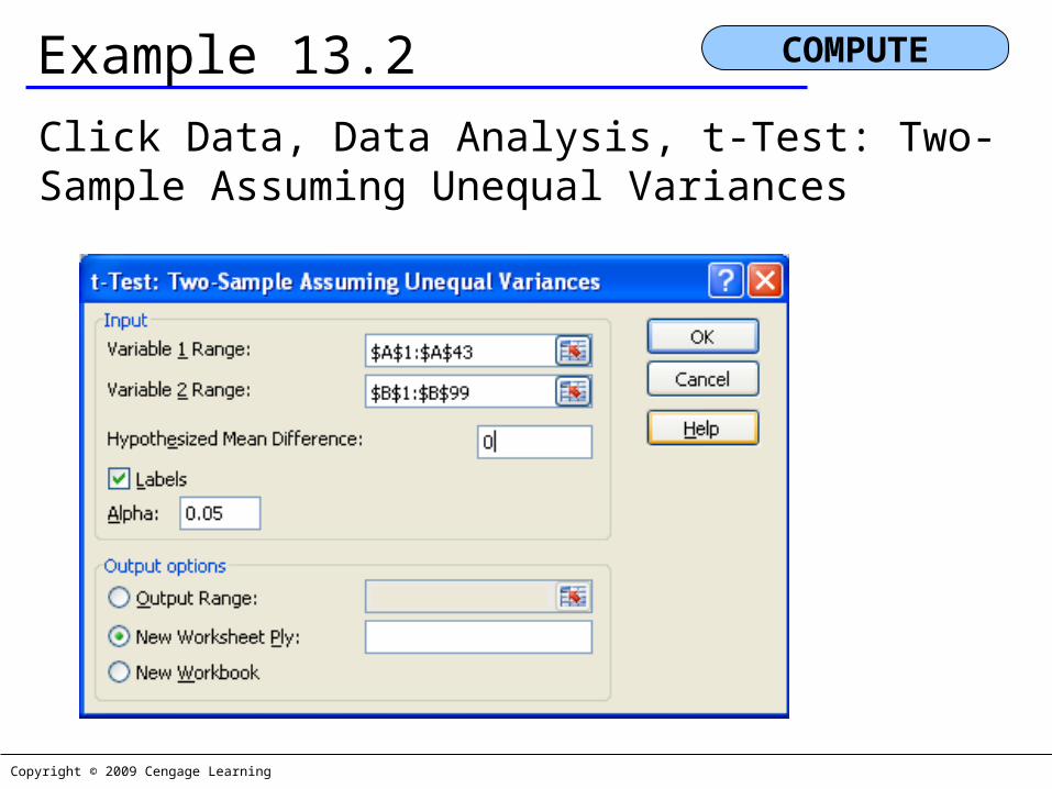
Click Data, Data Analysis, t-Test: Two-Sample Assuming Unequal Variances

COMPUTE


Example 13.2… COMPUTE

12

3456789

10111213

A B Ct-Test: Two-Sample Assuming Unequal Variances

Offspring OutsiderMean -0.10 1.24Variance 3.79 8.03Observations 42 98Hypothesized Mean Difference 0df 111t Stat -3.22P(T<=t) one-tail 0.0008t Critical one-tail 1.6587P(T<=t) two-tail 0.0017t Critical two-tail 1.9816


Example 13.2…The t-statistic is – 3.22 and its p-value is .0017. Accordingly, we conclude that there is sufficient evidence to infer that the mean times differ.

INTERPRET



We can also draw inferences about the difference between the two population means by calculating the confidence interval estimator. We use the unequal-variances confidence interval estimator of and a 95% confidence level.

We use the t-Estimate_2 Means (Uneq-Var) worksheet in the Estimators workbook or manually (Click here).



We activate the t-Estimate_2 Means (Uneq-Var) worksheet in the Estimators workbook and substitute the sample statistics and confidence level.

COMPUTE

12345678

A B C D E Ft-Estimate of the Difference Between Two Means (Unequal-Variances)

Sample 1 Sample 2 Confidence Interval EstimateMean -0.10 1.24 -1.34 ± 0.82Variance 3.79 8.03 Lower confidence limit -2.16Sample size 42 98 Upper confidence limit -0.51Degrees of freedom 110.75Confidence level 0.95



We estimate that the mean change in operating incomes for

outsiders exceeds the mean change in the operating income

for offspring lies between .51 and 2.16 percentage points.

INTERPRET


Checking the Required Condition

Both the equal-variances and unequal-variances techniques require that the populations be normally distributed. As before, we can check to see whether the requirement is satisfied by drawing the histograms of the data.


Checking the Required Condition: Example 13.1.

0

10

20

-5 0 5 10 15 20 More

Direct

Histogram

0

10

20

-5 0 5 10 15 20 More

Broker

Histogram


Checking the Required Condition: Example 13.2.

0

10

20

-4 -2 0 2 4

Offspring

Histogram

0

20

40

-4 -2 0 2 4 6 8 10

Outsider

Histogram


Violation of the Required ConditionWhen the normality requirement is unsatisfied, we can use a nonparametric technique-the Wilcoxon rank sum test for independent samples (Chapter 19)--to replace the equal-variances test of µ1-µ2 .

We have no alternative to the unequal-variances test of µ1-µ2 when the populations are very nonnormal.


Terminology

If all the observations in one sample appear in one column and all the observations of the second sample appear in another column, the data is unstacked.

If all the data from both samples is in the same column, the data is said to be stacked.


Developing an Understanding of Statistical Concepts 1The formulas in this section are relatively complicated. However, conceptually both test statistics are based on the techniques we introduced in Chapter 11 and repeated in Chapter 12.

That is, the value of the test statistic is the difference between the statistic and the hypothesized value of the parameter measured in terms of the standard error. errordardtanS

ParameterStatisticstatisticTest

−=


Developing an Understanding of Statistical Concepts 2As was the case with the interval estimator of p, the standard error must be estimated from the data for all inferential procedures introduced here.

The method we use to compute the standard error of depends on whether the population variances are equal. When they are equal we calculate and use the pooled variance estimator sp

2.

We are applying an important principle here, and we will so again in Section 13.5 and in later chapters. Where possible, it is advantageous to pool sample data to estimate the standard error.

21 xx −


Developing an Understanding of Statistical Concepts 2In the previous application, we are able to pool because we assume that the two samples were drawn from populations with a common variance.

Combining both samples increases the accuracy of the estimate. Thus, sp

2 is a better estimator of the common variance than either s1

2 or s22

separately.

When the two population variances are unequal, we cannot pool the data and produce a common estimator.

We must compute and use them to estimate σ12 and

σ22, respectively.


Identifying Factors I…

Factors that identify the equal-variances t-test and estimator of :


Identifying Factors II…

Factors that identify the unequal-variances t-test and estimator of :


“Ignorance ain’t what folks don’t know, it’s what folks know that just ain’t so”.

Will Rogers

Few things illustrate this more than how statistical results are interpreted.


Example 13.3Despite some controversy, scientists generally agree that

high-fiber cereals reduce the likelihood of various forms of

cancer.

However, one scientist claims that people who eat

high-fiber cereal for breakfast will consume, on average,

fewer calories for lunch than people who don't eat high-fiber

cereal for breakfast.


Example 13.3

If this is true, high-fiber cereal manufacturers will be able to

claim another advantage of eating their product--potential

weight reduction for dieters.

As a preliminary test of the claim, 150 people were

randomly selected and asked what they regularly eat for

breakfast and lunch.


Example 13.3

Each person was identified as either a consumer or a

nonconsumer of high-fiber cereal, and the number of calories

consumed at lunch was measured and recorded. Xm13-03

Can the scientist conclude at the 5% significance level that

his belief is correct?


Example 13.3

.

0)(:H 210 =μ−μ

0)(:H 211 <μ−μ

123456789

10111213

A B Ct-Test: Two-Sample Assuming Unequal Variances

Consumers NonconsumersMean 604.02 633.23Variance 4103 10670Observations 43 107Hypothesized Mean Difference 0df 123t Stat -2.09P(T<=t) one-tail 0.0193t Critical one-tail 1.6573P(T<=t) two-tail 0.0386t Critical two-tail 1.9794


Example 13.3

The value of the test statistic is −2.09.

The one-tail p-value is .0193.

We conclude that there is sufficient evidence to infer that consumers of high-fiber cereal do eat fewer calories at lunch than do nonconsumers.


Observational and Experimental DataFrom this result, we're inclined to believe that eating a high-fiber cereal at breakfast may be a way to reduce weight.

However, other interpretations are plausible.

For example, people who eat fewer calories are probably more health conscious, and such people are more likely to eat high-fiber cereal as part of a healthy breakfast.

In this interpretation, high-fiber cereals do not necessarily lead to fewer calories at lunch.


Observational and Experimental DataInstead another factor, general health consciousness, leads to both fewer calories at lunch and high-fiber cereal for breakfast.

Notice that the conclusion of the statistical procedure is unchanged.

On average, people who eat high-fiber cereal consume fewer calories at lunch. However, because of the way the data were gathered, we have more difficulty interpreting this result.


Observational and Experimental DataFrom the result in Example 13.3, we're inclined to believe

that eating a high-fiber cereal at breakfast may be a way to reduce weight.

However, other interpretations are possible. For example, people

Who eat fewer calories at lunch are probably more health conscious, and such people are more likely to eat high-fiber cereal as part of a healthy breakfast.

In this interpretation, high-fiber cereals do not necessarily lead to

Fewer calories at lunch. Instead another factor, general health

consciousness, leads to both fewer calories at lunch and high-fiber

cereal for breakfast.


Observational and Experimental DataSuppose that we redo Example 13.3 using the experimental approach.

We randomly select 150 people to participate in the experiment.

We randomly assign 75 to eat high-fiber cereal for breakfast and the other 75 to eat something else.

We then record the number of calories each person consumes at lunch.


Observational and Experimental DataBoth groups should be similar in all other dimensions, including health consciousness. (Larger sample sizes increase the likelihood that the two groups will be similar.)

If the statistical result is about the same as in Example 13.3, we may have some valid reason to believe that high-fiber cereal at breakfast leads to a decrease in caloric intake at lunch.


Matched Pairs Experiment…

Previously when comparing two populations, we examined independent samples.

If, however, an observation in one sample is matched with an observation in a second sample, this is called a matched pairs experiment.

To help understand this concept, let’s consider Example 13.4


Example 13.4

In the last few years a number of web-based companies that offer job placement services have been created.

The manager of one such company wanted to investigate the job offers recent MBAs were obtaining.

In particular, she wanted to know whether finance majors were being offered higher salaries than marketing majors.


Example 13.4

In a preliminary study she randomly sampled 50 recently graduated MBAs half of whom majored in finance and half in marketing.

From each she obtained the highest salary (including benefits) offer (Xm13-04).

Can we infer that finance majors obtain higher salary offers than do marketing majors among MBAs?


Example 13.4The parameter is the difference between two means (where µ1 = mean highest salary offer to finance majors and µ2 = mean highest salary offer to marketing majors).

Because we want to determine whether finance majors are offered higher salaries, the alternative hypothesis will specify that is greater than.

Calculation of the F-test of two variances indicates the use the equal-variances test statistic.

IDENTIFY


Example 13.4

The hypotheses are

The Excel output is:

0)(:H 210 =μ−μ

0)(:H 211 >μ−μ

IDENTIFY


Example 13.4

12

3456789

1011121314

A B Ct-Test: Two-Sample Assuming Equal Variances

Finance MarketingMean 65,624 60,423Variance 360,433,294 262,228,559Observations 25 25Pooled Variance 311,330,926Hypothesized Mean Difference 0df 48t Stat 1.04P(T<=t) one-tail 0.1513t Critical one-tail 1.6772P(T<=t) two-tail 0.3026t Critical two-tail 2.0106

COMPUTE


Example 13.4

The value of the test statistic (t =1.04) and its p-value (.1513) indicate that there is very little evidence to support the hypothesis that finance majors attract higher salary offers than marketing majors.

INTERPRET


Example 13.4

We have some evidence to support the alternative hypothesis, but not enough.

Note that the difference in sample means is

= (65,624 -60,423) = 5,201

INTERPRET

21 xx −


Example 13.5Suppose now that we redo the experiment in the following way.

We examine the transcripts of finance and marketing MBA majors.

We randomly sample a finance and a marketing major whose grade point average (GPA) falls between 3.92 and 4 (based on a maximum of 4).

We then randomly sample a finance and a marketing major whose GPA is between 3.84 and 3.92.


Example 13.5We continue this process until the 25th pair of finance and marketing majors are selected whose GPA fell between 2.0 and 2.08.

(The minimum GPA required for graduation is 2.0.)

As we did in Example 13.4, we recorded the highest salary offer . Xm13-05

Can we conclude from these data that finance majors draw larger salary offers than do marketing majors?


Example 13.5The experiment described in Example 13.4 is one in which the samples are independent. That is, there is no relationship between the observations in one sample and the observations in the second sample. However, in this example the experiment was designed in such a way that each observation in one sample is matched with an observation in the other sample. The matching is conducted by selecting finance and marketing majors with similar GPAs. Thus, it is logical to compare the salary offers for finance and marketing majors in each group. This type of experiment is called matched pairs.

IDENTIFY


Example 13.5

For each GPA group, we calculate the matched pair difference between the salary offers for finance and marketing majors.

IDENTIFY


Example 13.5

The numbers in black are the original starting salary data (Xm13-05) ; the numbers in blue were calculated.

although a student is either in Finance OR in Marketing (i.e. independent), that the data is grouped in this fashion makes it a matched pairs experiment (i.e. the two students in group #1 are ‘matched’ by their GPA range

the difference of the means is equal to the mean of the differences, hence we will consider the “mean of the paired differences” as our parameter of interest:

IDENTIFY


Example 13.5

Do Finance majors have higher salary offers than Marketing majors?

Since:

We want to research this hypothesis: H1:

(and our null hypothesis becomes H0: )

IDENTIFY


Test Statistic for

The test statistic for the mean of the population of differences ( ) is:

which is Student t distributed with nD–1 degrees of freedom, provided that the differences are normally distributed.

IDENTIFY





COMPUTE


Example 13.5

Click Data, Data Analysis, t-Test: Paired Two- Sample for Means

COMPUTE


Example 13.5 COMPUTE

12

3456789

1011121314

A B Ct-Test: Paired Two Sample for Means

Finance MarketingMean 65,438 60,374Variance 444,981,810 469,441,785Observations 25 25Pearson Correlation 0.9520Hypothesized Mean Difference 0df 24t Stat 3.81P(T<=t) one-tail 0.0004t Critical one-tail 1.7109P(T<=t) two-tail 0.0009t Critical two-tail 2.0639


Example 13.5

The p-value is .0004. There is overwhelming evidence that Finance majors do obtain higher starting salary offers than their peers in Marketing.

INTERPRET


Example 13.6 Confidence Interval Estimator for µD

We can derive the confidence interval estimator for algebraically as:

1234567

A B Ct-Estimate: Mean

DifferenceMean 5065Standard Deviation 6647LCL 2321UCL 7808


Checking the Required Condition

The population of differences are required to be normally distributed. As before, we can check to see whether the requirement is satisfied by drawing the histogram of the differences.

.

Histogram

0

5

10

0 5000 10000 15000 20000

Difference

Frequency


Violation of the Required Condition If the differences are very nonnormal, we cannot use the t-test of µD.

We can, however, employ a nonparametric technique--the Wilcoxon signed rank sum test for matched pairs, which we present in Chapter 19.


Independent Samples or Matched Pairs: Which Experimental Design is Better?

Examples 13.4 and 13.5 demonstrated that the experimental design is an important factor in statistical inference.

However, these two examples raise several questions about experimental designs. 1 Why does the matched pairs experiment result in rejecting the null hypothesis, whereas the independent samples experiment could not?



2 Should we always use the matched pairs experiment? In particular, are there disadvantages to its use? 3 How do we recognize when a matched pairs experiment has been performed?



1 The matched pairs experiment worked in Example 13.5 by reducing the variation in the data.

To understand this point, examine the statistics from both examples. In Example 13.4, we found

and in Example 13.5

201,5xx 21 =−

065,5xD =



Thus, the numerators of the two test statistics were quite similar.

However, the test statistic in Example 13.5 was much larger than the test statistic in Example 13.4 because of the standard errors.



In Example 13.4, we calculated

Example 13.5 produced

926,330,311s 2p =

991,4n

1

n

1s

21

2p =⎟⎟

⎠

⎞⎜⎜⎝

⎛+

647,6sD =

329,1n

s

D

D =



2 Will the matched pairs experiment always produce a larger test statistic than the independent samples experiment? The answer is, “Not necessarily.”

Suppose that in our example we found that companies did not consider grade point averages when making decisions about how much to offer the MBA graduates.

In such circumstances, the matched pairs experiment would result in no significant decrease in variation when compared to independent samples.



3 As you've seen, in this course we deal with questions arising from experiments that have already been conducted.

Thus, one of your tasks is to determine the appropriate test statistic.

In the case of comparing two populations of interval data, you must decide whether the samples are independent (in which case the parameter is) or matched pairs (in which case the parameter is) to select the correct test statistic.



To help you do so, we suggest you ask and answer the following question:

Does some natural relationship exist between each pair of observations that provides a logical reason to compare the first observation of sample 1 with the first observation of sample 2, the second observation of sample 1 with the second observation of sample 2, and so on?

If so, the experiment was conducted by matched pairs. If not, it was conducted using independent samples.


Developing an Understanding of Statistical Concepts 1Two of the most important principles in statistics were applied in this section.

The first is the concept of analyzing sources of variation. In Examples 13.4 and 13.5, we showed that by reducing the variation between salary offers in each sample we were able to detect a real difference between the two majors..


Developing an Understanding of Statistical Concepts 1This was an application of the more general procedure of analyzing data and attributing some fraction of the variation to several sources.

In Example 13.5, the two sources of variation were the GPA and the MBA major. However, we were not interested in the variation between graduates with differing GPAs.

Instead we only wanted to eliminate that source of variation, making it easier to determine whether finance majors draw larger salary offers.


Developing an Understanding of Statistical Concepts 1In Chapter 14, we will introduce a technique called the analysis of variance which does what its name suggests; it analyzes sources of variation in an attempt to detect real differences.

In most applications of this procedure, we will be interested in each source of variation and not simply in reducing one source.

We refer to the process as explaining the variation. The concept of explained variation also will be applied in Chapters 16 - 18.


Developing an Understanding of Statistical Concepts 2The second principle demonstrated in this section is that statistics practitioners can design data-gathering procedures in such a way that they can analyze sources of variation.

Before conducting the experiment in Example 13.5, the statistics practitioner suspected that there were large differences between graduates with different GPAs.


Developing an Understanding of Statistical Concepts 2Consequently, the experiment was organized so that the effects of those differences were mostly eliminated.

It is also possible to design experiments that allow for easy detection of real differences and minimize the costs of data gathering.


Identifying Factors…

Factors that identify the t-test and estimator of :


Inference about the ratio of two variancesSo far we’ve looked at comparing measures of central location, namely the mean of two populations.

When looking at two population variances, we consider the ratio of the variances, i.e. the parameter of interest to us is:

The sampling statistic: is F distributed with

degrees of freedom.


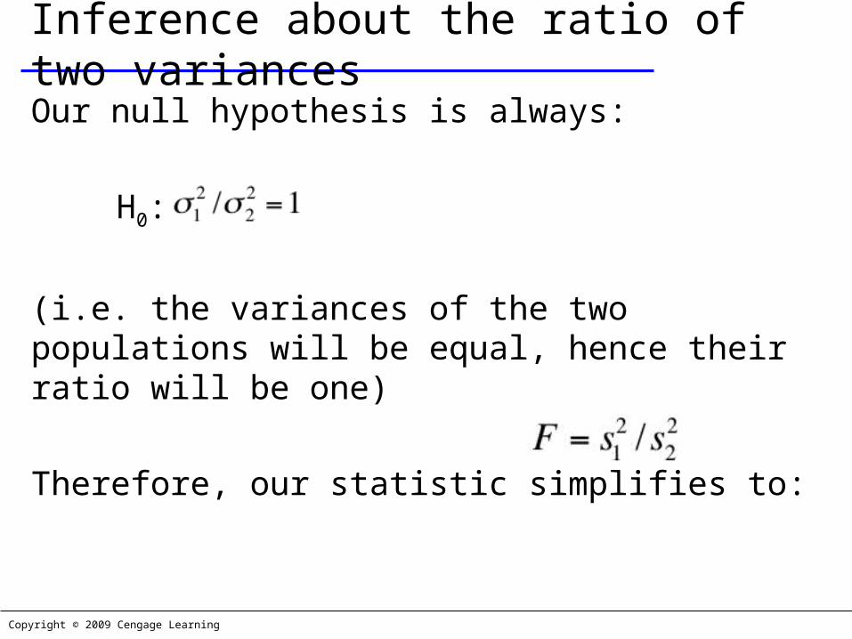
Inference about the ratio of two variancesOur null hypothesis is always:

H0:

(i.e. the variances of the two populations will be equal, hence their ratio will be one)

Therefore, our statistic simplifies to:


Example 13.7In Example 12.3, we applied the chi-squared test of a variance to determine whether there was sufficient evidence

to conclude that the population variance was less than 1.0.

Suppose that the statistics practitioner also collected data

from another container-filling machine and recorded the fills

of a randomly selected sample.

Can we infer at the 5% significance level that the second

machine is superior in its consistency?

IDENTIFY


Example 13.7

The problem objective is to compare two populations where

the data are interval.

Because we want information about the consistency of the

two machines, the parameter we wish to test is σ1

2 / σ22,

where σ12 is the variance of machine 1

and σ22, is the

variance for machine 2.

IDENTIFY


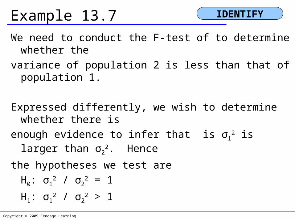
Example 13.7We need to conduct the F-test of to determine whether the

variance of population 2 is less than that of population 1.

Expressed differently, we wish to determine whether there is

enough evidence to infer that is σ12 is

larger than σ22. Hence

the hypotheses we test areH0: σ1

2 / σ22 = 1

H1: σ12 / σ2

2 > 1

IDENTIFY





COMPUTE


Example 13.7

Click Data, Data Analysis, F-Test Two-Sample for Variances.

COMPUTE


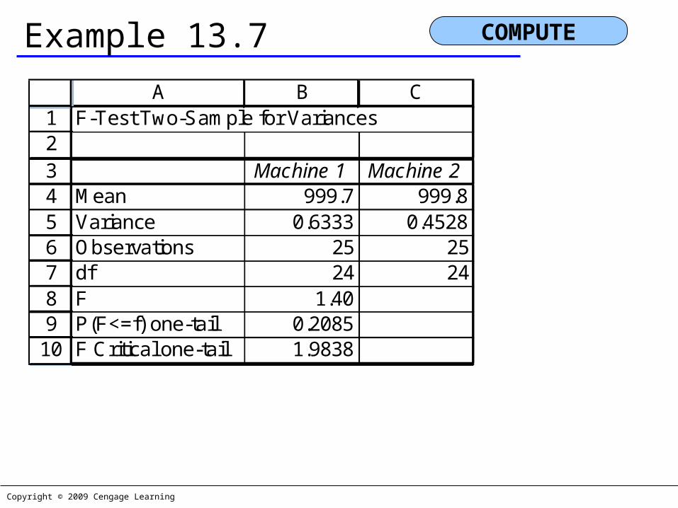
Example 13.7

COMPUTE

123456789

10


Machine 1 Machine 2Mean 999.7 999.8Variance 0.6333 0.4528Observations 25 25df 24 24F 1.40P(F<=f) one-tail 0.2085F Critical one-tail 1.9838


Example 13.7

There is not enough evidence to infer that the variance of

machine 2 is less than the variance of machine 1.

INTERPRET


Example 13.8

Determine the 95% confidence interval estimate of the ratio

of the two population variances in Example 13.7.

The confidence interval estimator for σ12

/ σ22 is:





COMPUTE


Example 13.8Open the F-Estimator_2 Variances worksheet in the Estimators workbook and substitute sample variances, samples sizes, and the confidence level.

That is, we estimate that σ12 / σ2

2 lies between .6164 and 3.1741Note that one (1.00) is in this interval.

COMPUTE

123456

A B C D EF-Estimate of the Ratio of Two Variances

Sample 1 Sample 2 Confidence Interval EstimateSample variance 0.6333 0.4528 Lower confidence limit 0.6164Sample size 25 25 Upper confidence limit 3.1741Confidence level 0.95


Identifying Factors

Factors that identify the F-test and estimator of :


Difference Between Two Population ProportionsWe will now look at procedures for drawing inferences about the difference between populations whose data are nominal (i.e. categorical).

As mentioned previously, with nominal data, calculate proportions of occurrences of each type of outcome. Thus, the parameter to be tested and estimated in this section is the difference between two population proportions: p1–p2.


Statistic and Sampling Distribution…To draw inferences about the the parameter p1–p2, we take samples of population, calculate the sample proportions and look at their difference.

is an unbiased estimator for p1–p2.

x1 successes in a sample of size n1 from population 1


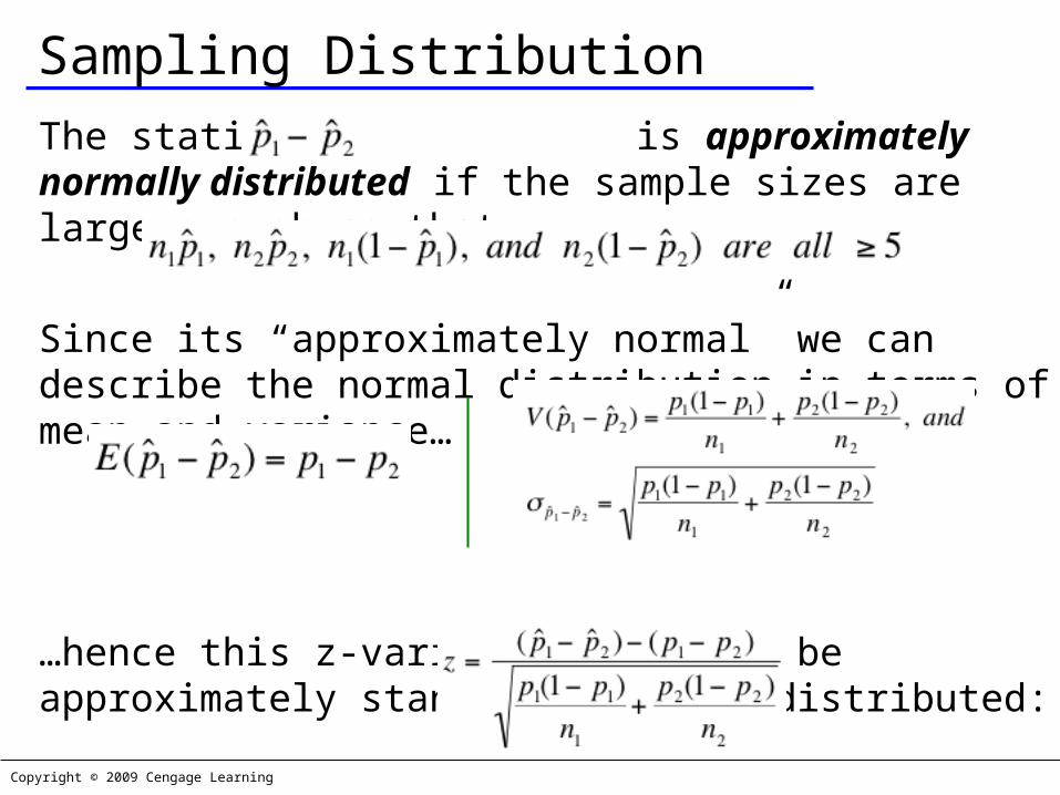
Sampling DistributionThe statistic is approximately normally distributed if the sample sizes are large enough so that:

Since its “approximately normal” we can describe the normal distribution in terms of mean and variance…

…hence this z-variable will also be approximately standard normally distributed:


Testing and Estimating p1–p2

Because the population proportions (p1 & p2) are unknown, the standard error:

is unknown. Thus, we have two different estimators for the standard error of , which depend upon the null hypothesis. We’ll look at these cases on the next slide…


Test Statistic for p1–p2

There are two cases to consider…


Example 13.9

The General Products Company produces and sells a bath soap, which is not selling well.

Hoping to improve sales General products decided to introduce more attractive packaging.

The company’s advertising agency developed two new designs.


Example 13.9The first design features several bright colors to distinguish it from other brands.

The second design is light green in color with just the company’s logo on it.

As a test to determine which design is better the marketing manager selected two supermarkets.

In one supermarket the soap was packaged in a box using the first design and in the second supermarket the second design was used.


Example 13.9

The product scanner at each supermarket tracked every buyer of soap over a one week period.

The supermarkets recorded the last four digits of the scanner code for each of the five brands of soap the supermarket sold. Xm13-09

The code for the General Products brand of soap is 9077(the other codes are 4255, 3745, 7118, and 8855).


Example 13.9

After the trial period the scanner data were transferred to a computer file.

Because the first design is more expensive management has decided to use this design only if there is sufficient evidence to allow them to conclude that it is better.

Should management switch to the brightly-colored design or the simple green one?


Example 13.9The problem objective is to compare two populations. The first is the population of soap sales in supermarket 1 and the second is the population of soap sales in supermarket 2.

The data are nominal because the values are “buy General Products soap” and “buy other companies’ soap.”

These two factors tell us that the parameter to be tested is the difference between two population proportions p1-p2 (where p1 and p2 are the proportions of soap sales that are a General Products brand in supermarkets 1 and 2, respectively.

IDENTIFY


Example 13.9Because we want to know whether there is enough evidence to adopt the brightly-colored design, the alternative hypothesis is

H1: (p1 – p2) > 0

The null hypothesis must be H0: (p1 – p2) = 0

which tells us that this is an application of Case 1. Thus, the test statistic is

IDENTIFY

⎟⎟⎠

⎞⎜⎜⎝

⎛+−

−=

21

21

n

1

n

1)p̂1(p̂

)p̂p̂(z





COMPUTE


Example 13.9

Click Add-Ins, Data Analysis Plus, Z-Test: 2 Proportions

COMPUTE


Example 13.9

COMPUTE

123456789

1011

A B Cz-Test: Two Proportions

Supermarket 1 Supermarket 2Sample Proportions 0.1991 0.1493Observations 904 1038Hypothesized Difference 0z Stat 2.90P(Z<=z) one tail 0.0019z Critical one-tail 1.6449P(Z<=z) two-tail 0.0038z Critical two-tail 1.96


Example 13.9

The value of the test statistic is z = 2.90; its p-value is .0019. There is enough evidence to infer that the brightly-colored design is more popular than the simple design. As a result, it is recommended that management switch to the first design.

INTERPRET


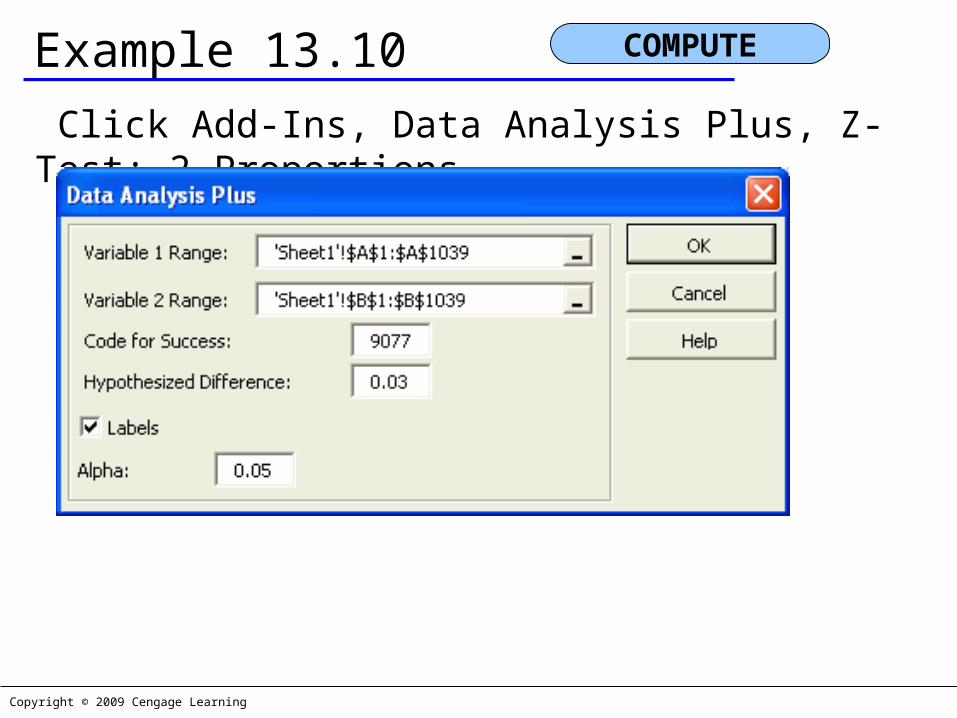
Example 13.10

Suppose in our test marketing of soap packages scenario that instead of just a difference between the two package versions, the brightly colored design had to outsell the simple design by at least 3%


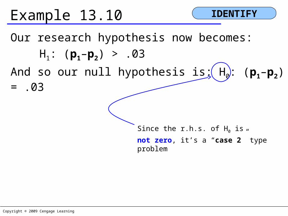
Example 13.10

Our research hypothesis now becomes:H1: (p1–p2) > .03

And so our null hypothesis is: H0: (p1–p2) = .03

IDENTIFY

Since the r.h.s. of H0 is

not zero, it’s a “case 2” type problem


Example 13.10

Click Add-Ins, Data Analysis Plus, Z-Test: 2 Proportions

COMPUTE


Example 13.10

COMPUTE

123456789

1011

A B Cz-Test: Two Proportions

Supermarket 1 Supermarket 2Sample Proportions 0.1991 0.1493Observations 904 1038Hypothesized Difference 0.03z Stat 1.14P(Z<=z) one tail 0.1261z Critical one-tail 1.6449P(Z<=z) two-tail 0.2522z Critical two-tail 1.96


Example 13.10

There is not enough evidence to infer that the brightly colored design outsells the other design by 3% or more.

INTERPRET



The confidence interval estimator for p1–p2 is given by:

and as you may suspect, its valid when…


Example 13.11

To help estimate the difference in profitability, the

Marketing manager in Examples 13.9 and 13.10 would

like to estimate the difference between the two

proportions. A confidence level of 95% is suggested.





COMPUTE


Example 13.11Click Add-Ins, Data Analysis Plus, Z-Estimate: 2 Proportions

COMPUTE


Example 13.11

COMPUTE

12345678

A B C Dz-Estimate: Two Proportions

Supermarket 1 Supermarket 2Sample Proportions 0.1991 0.1493Observations 904 1038

LCL 0.0159UCL 0.0837


Identifying Factors…

Factors that identify the z-test and estimator for p1–p2

copyright © 2009 cengage learning chapter 13 inference about comparing two populations

Documents