copyright © 2011 pearson education, inc. slide 4.3-1 4.3 rational equations, inequalities,...
TRANSCRIPT
Copyright © 2011 Pearson Education, Inc. Slide 4.3-1
4.3 Rational Equations, Inequalities, Applications, and Models
• Solving Rational Equations and Inequalities– at least one variable in the denominator
– may be undefined for certain values where the denominator is 0
– identify those values that make the equation (or inequality) undefined
– when solving rational equations, you generally multiply both sides by a common denominator
– when solving rational inequalities, you generally get 0 on one side, then rewrite the rational expression as a single fraction
Copyright © 2011 Pearson Education, Inc. Slide 4.3-2
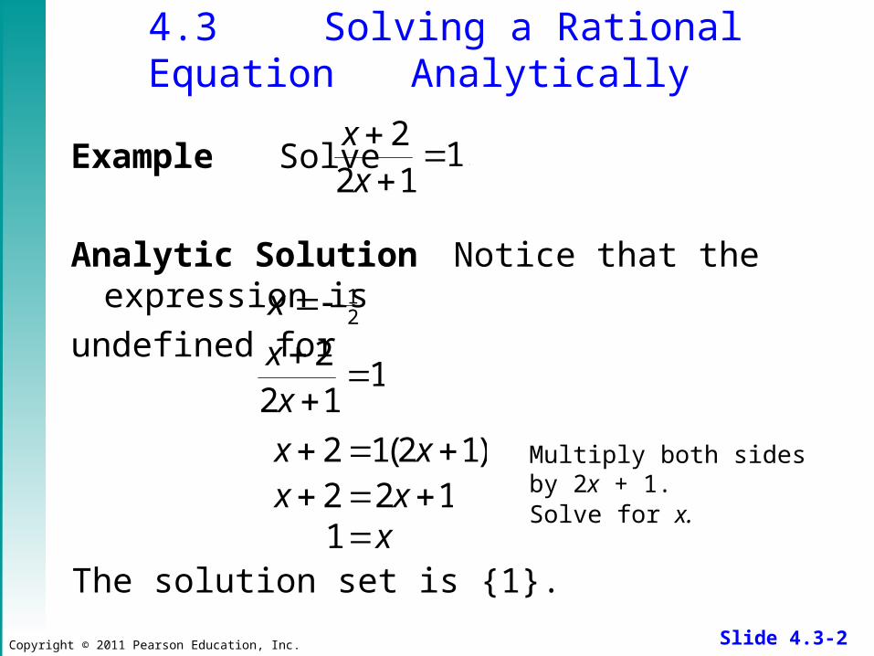
4.3 Solving a Rational Equation Analytically
Example Solve
Analytic Solution Notice that the expression is
undefined for
.1122
xx
.21x
1122
xx
Multiply both sides by 2x + 1.)12(12 xx
xxx
1122
Solve for x.
The solution set is {1}.
Copyright © 2011 Pearson Education, Inc. Slide 4.3-3
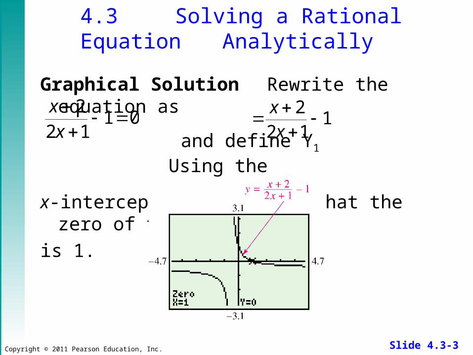
4.3 Solving a Rational Equation Analytically
Graphical Solution Rewrite the equation as
and define Y1 Using the
x-intercept method shows that the zero of the function
is 1.
01122
xx
.1122
xx
Copyright © 2011 Pearson Education, Inc. Slide 4.3-4
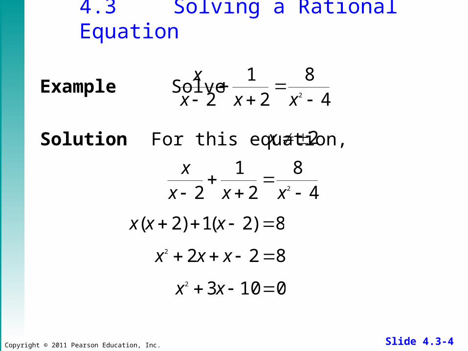
4.3 Solving a Rational Equation
Example Solve
Solution For this equation,
.4
82
12 2
xxxx
.2x
48
21
2 2
xxxx
8)2(1)2( xxx
8222 xxx
01032 xx

Copyright © 2011 Pearson Education, Inc. Slide 4.3-5
4.3 Solving a Rational Equation
But, x = 2 is not in the domain of the original
equation and, therefore, must be rejected. The
solution set is {–5}.
2or5
0)2)(5(
xx
xx
Copyright © 2011 Pearson Education, Inc. Slide 4.3-6
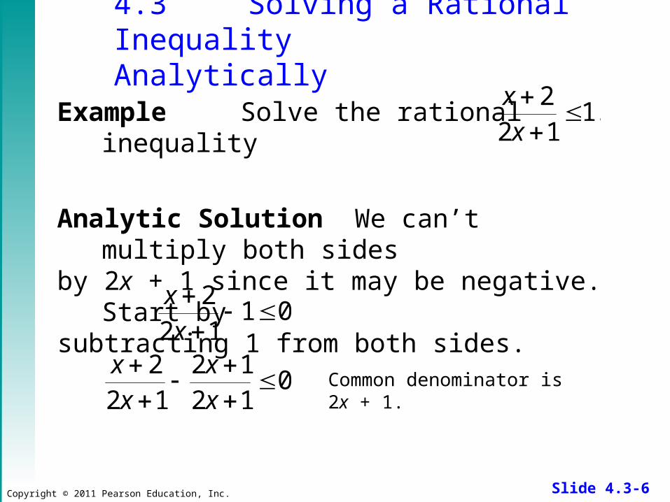
4.3 Solving a Rational Inequality Analytically
Example Solve the rational inequality
Analytic Solution We can’t multiply both sides by 2x + 1 since it may be negative. Start by subtracting 1 from both sides.
.1122
xx
01212
122
01122
xx
xx
xx
Common denominator is 2x + 1.
Copyright © 2011 Pearson Education, Inc. Slide 4.3-7
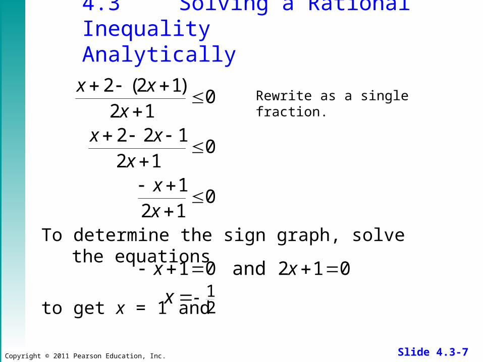
4.3 Solving a Rational Inequality Analytically
To determine the sign graph, solve the equations
to get x = 1 and
0121
012
122
012
)12(2
xx
xxx
xxx
Rewrite as a single fraction.
012and01 xx
.21x
Copyright © 2011 Pearson Education, Inc. Slide 4.3-8
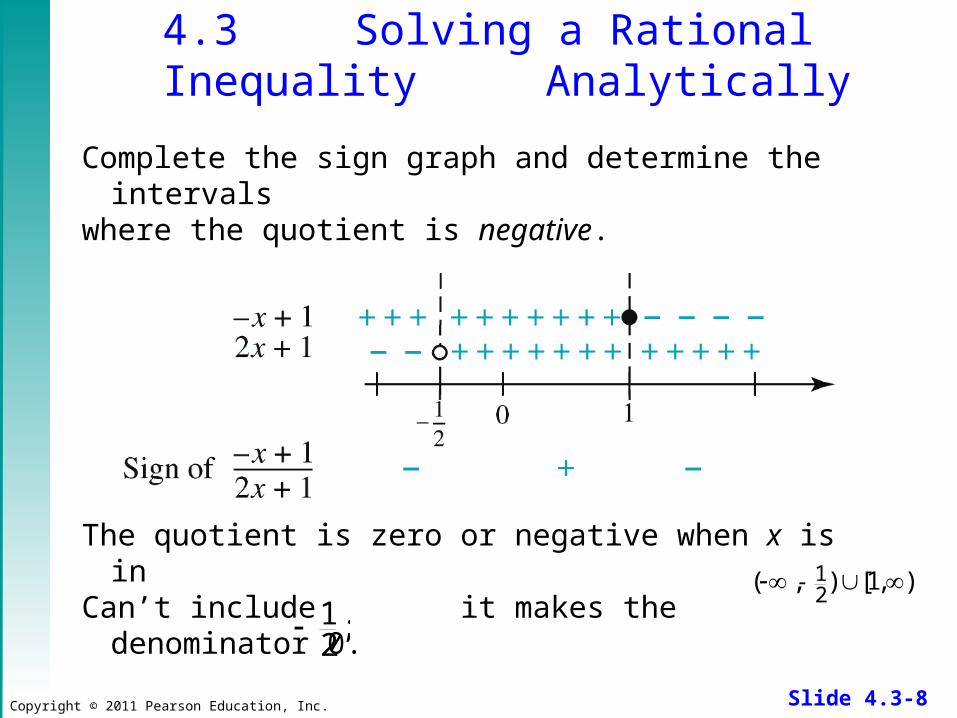
4.3 Solving a Rational Inequality Analytically
Complete the sign graph and determine the intervalswhere the quotient is negative.
The quotient is zero or negative when x is in Can’t include it makes the denominator 0.
).,1[),(21
;21
Copyright © 2011 Pearson Education, Inc. Slide 4.3-9
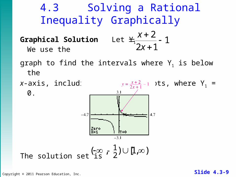
4.3 Solving a Rational Inequality Graphically
Graphical Solution Let Y1 We use the
graph to find the intervals where Y1 is below the
x-axis, including the x-intercepts, where Y1 = 0.
The solution set is
.1122
xx
).,1[),(21
Copyright © 2011 Pearson Education, Inc. Slide 4.3-10
4.3 Solving Equations Involving Rational Functions
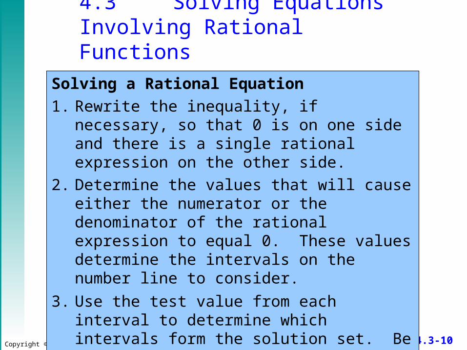
Solving a Rational Equation
1. Rewrite the inequality, if necessary, so that 0 is on one side and there is a single rational expression on the other side.
2. Determine the values that will cause either the numerator or the denominator of the rational expression to equal 0. These values determine the intervals on the number line to consider.
3. Use the test value from each interval to determine which intervals form the solution set. Be sure to check endpoints.
Copyright © 2011 Pearson Education, Inc. Slide 4.3-11
4.3 Models and Applications of Rational Functions: Analyzing Traffic Intensity
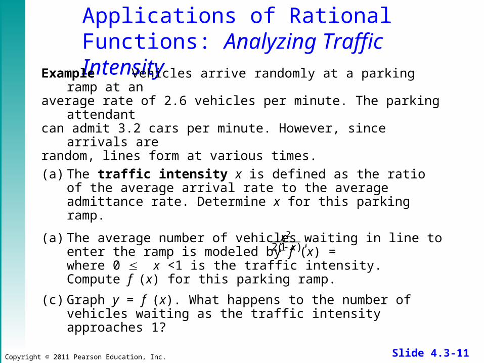
Example Vehicles arrive randomly at a parking ramp at an
average rate of 2.6 vehicles per minute. The parking attendant can admit 3.2 cars per minute. However, since arrivals are random, lines form at various times.
(a) The traffic intensity x is defined as the ratio of the average arrival rate to the average admittance rate. Determine x for this parking ramp.
(a) The average number of vehicles waiting in line to enter the ramp is modeled by f (x) = where 0 x <1 is the traffic intensity. Compute f (x) for this parking ramp.
(c) Graph y = f (x). What happens to the number of vehicles waiting as the traffic intensity approaches 1?
2
2(1 ) ,xx
Copyright © 2011 Pearson Education, Inc. Slide 4.3-12
4.3 Models and Applications of Rational Functions: Analyzing Traffic Intensity
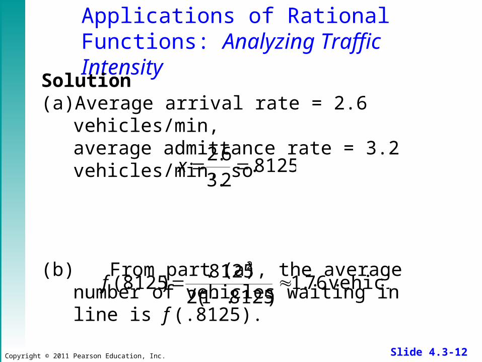
Solution(a) Average arrival rate = 2.6 vehicles/min,
average admittance rate = 3.2 vehicles/min, so
(b) From part (a), the average number of vehicles waiting in line is f (.8125).
.8125.2.36.2 x
vehicles76.1)8125.1(2
8125.)8125(.
2
f
Copyright © 2011 Pearson Education, Inc. Slide 4.3-13
4.3 Models and Applications of Rational Functions: Analyzing Traffic
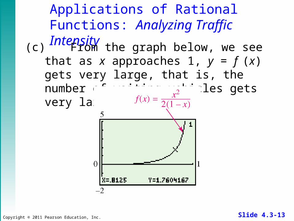
Intensity(c) From the graph below, we see that as x
approaches 1, y = f (x) gets very large, that is, the number of waiting vehicles gets very large.
Copyright © 2011 Pearson Education, Inc. Slide 4.3-14
4.3 Models and Applications of Rational Functions: Optimization Problem
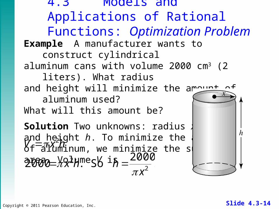
Example A manufacturer wants to construct cylindrical aluminum cans with volume 2000 cm3 (2 liters). What radius and height will minimize the amount of aluminum used? What will this amount be?
Solution Two unknowns: radius xand height h. To minimize the amount of aluminum, we minimize the surface area. Volume V is
.2000
So.2000 22
2
xhhx
hxV
Copyright © 2011 Pearson Education, Inc. Slide 4.3-15
4.3 Models and Applications of Rational Functions: Optimization Problem
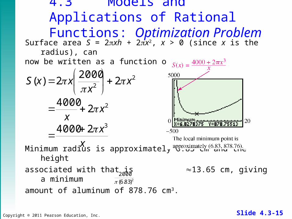
Surface area S = 2xh + 2x2, x > 0 (since x is the radius), can now be written as a function of x.
Minimum radius is approximately 6.83 cm and the height
associated with that is 13.65 cm, giving a minimum
amount of aluminum of 878.76 cm3.
xx
xx
xx
xxS
3
2
22
24000
24000
22000
2)(
2)83.6(2000
Copyright © 2011 Pearson Education, Inc. Slide 4.3-16
4.3 Inverse Variation
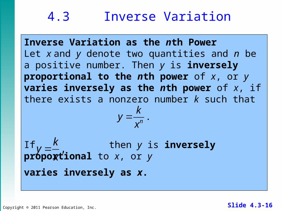
Inverse Variation as the nth PowerLet x and y denote two quantities and n be a positive number. Then y is inversely proportional to the nth power of x, or y varies inversely as the nth power of x, if there exists a nonzero number k such that
If then y is inversely proportional to x, or y
varies inversely as x.
.n
ky
x
,k
yx
Copyright © 2011 Pearson Education, Inc. Slide 4.3-17
4.3 Modeling the Intensity of Light
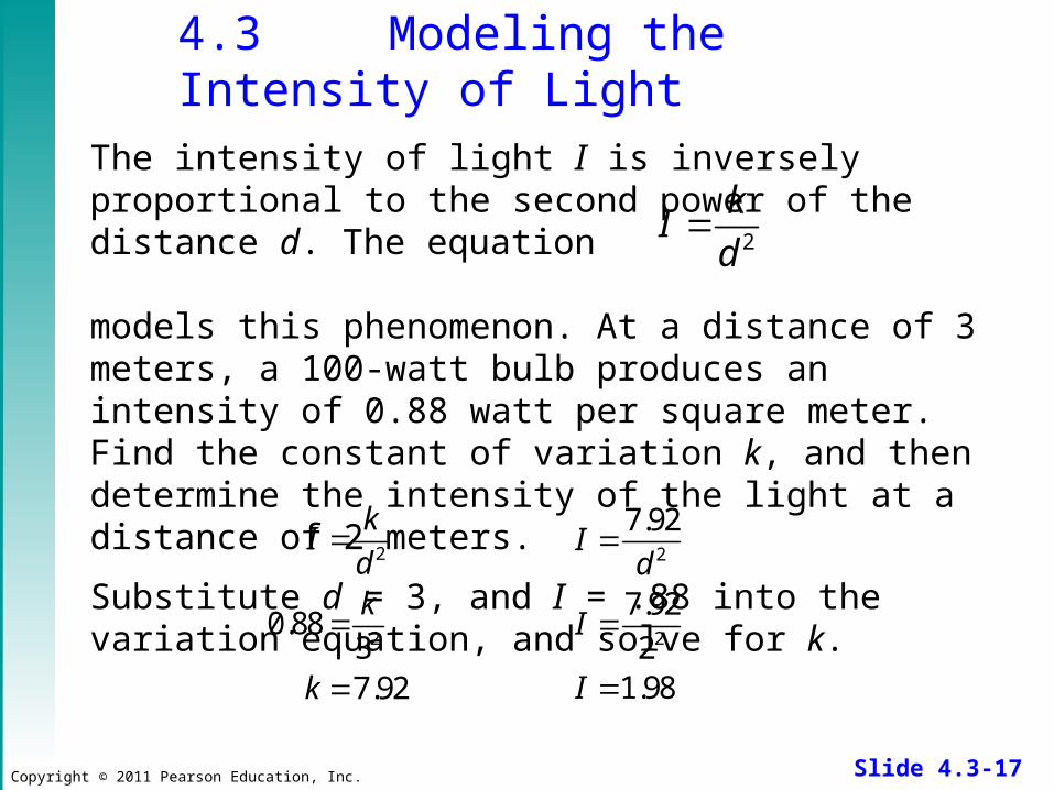
The intensity of light I is inversely proportional to the second power of the distance d. The equation
models this phenomenon. At a distance of 3 meters, a 100-watt bulb produces an intensity of 0.88 watt per square meter. Find the constant of variation k, and then determine the intensity of the light at a distance of 2 meters.
Substitute d = 3, and I = .88 into the variation equation, and solve for k.
2
kI
d
2
20.88
37.92
kI
dk
k
2
2
7.92
7.92
21.98
Id
I
I
Copyright © 2011 Pearson Education, Inc. Slide 4.3-18
4.3 Joint Variation
Joint VariationLet m and n be real numbers. Then z varies jointly as the nth power of x and the mth power of y if a nonzero real number k exists such that
z = kxnym.
Copyright © 2011 Pearson Education, Inc. Slide 4.3-19
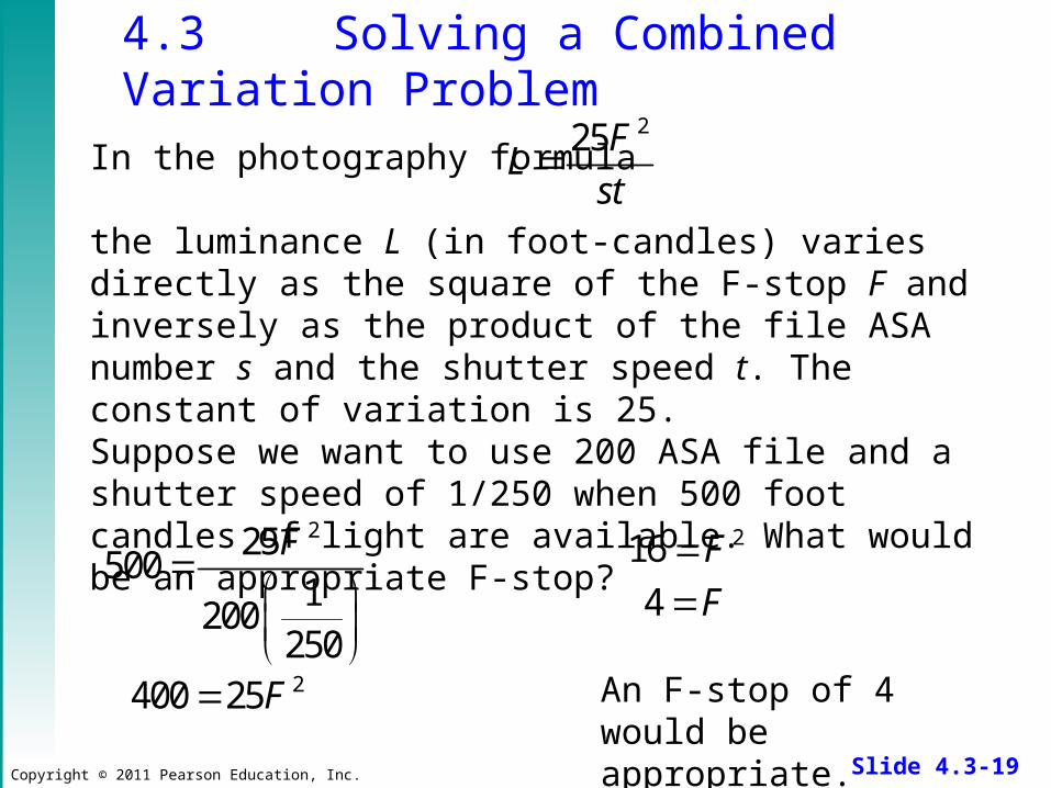
4.3 Solving a Combined Variation Problem
In the photography formula
the luminance L (in foot-candles) varies directly as the square of the F-stop F and inversely as the product of the file ASA number s and the shutter speed t. The constant of variation is 25.Suppose we want to use 200 ASA file and a shutter speed of 1/250 when 500 foot candles of light are available. What would be an appropriate F-stop?
225FL
st
225500
1200
250
F
2400 25F
216 F4 F
An F-stop of 4 would be appropriate.
Copyright © 2011 Pearson Education, Inc. Slide 4.3-20
4.3 Rate of Work
Rate of WorkIf 1 task can be completed in x units of time, then the rate of work is 1/x task per time unit.
Copyright © 2011 Pearson Education, Inc. Slide 4.3-21
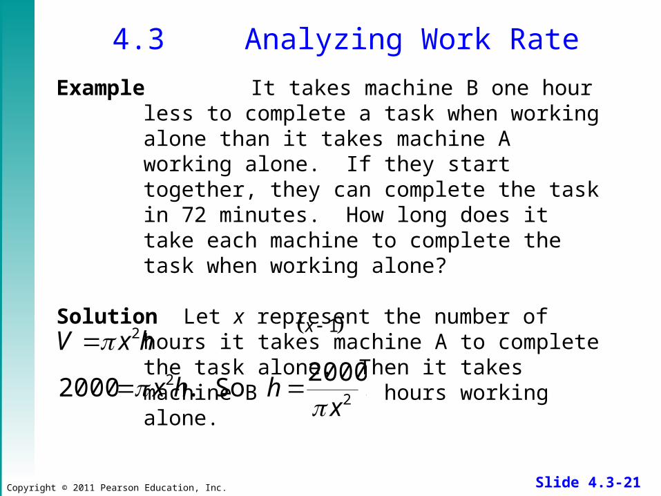
4.3 Analyzing Work Rate
Example It takes machine B one hour less to complete a task when working alone than it takes machine A working alone. If they start together, they can complete the task in 72 minutes. How long does it take each machine to complete the task when working alone?
Solution Let x represent the number of hours it takes machine A to complete the task alone. Then it takes machine B hours working alone.
.2000
So.2000 22
2
xhhx
hxV
1x
Copyright © 2011 Pearson Education, Inc. Slide 4.3-22
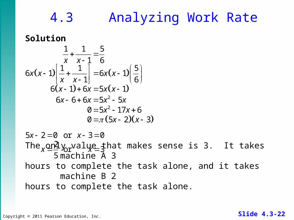
4.3 Analyzing Work Rate
Solution
The only value that makes sense is 3. It takes machine A 3 hours to complete the task alone, and it takes machine B 2 hours to complete the task alone.
2
2
1 1 5
1 61 1 5
6 1 6 11 6
6 1 6 5 16 6 6 5 5
0 5 17 60 5 2 3
x x
x x x xx xx x x xx x x x
x xx x
5 2 0 or 3 02
or 35
x x
x x