copyright © 2011 pearson education, inc. statistical tests chapter 16
TRANSCRIPT

Copyright © 2011 Pearson Education, Inc.
Statistical Tests
Chapter 16
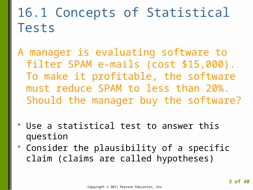
16.1 Concepts of Statistical Tests
A manager is evaluating software to filter SPAM e-mails (cost $15,000). To make it profitable, the software must reduce SPAM to less than 20%. Should the manager buy the software?
Use a statistical test to answer this question Consider the plausibility of a specific claim
(claims are called hypotheses)
Copyright © 2011 Pearson Education, Inc.
3 of 40

16.1 Concepts of Statistical Tests
Null and Alternative Hypotheses
Statistical hypothesis: claim about a parameter of a population.
Null hypothesis (H0): specifies a default course of action, preserves the status quo.
Alternative hypothesis (Ha): contradicts the assertion of the null hypothesis.
Copyright © 2011 Pearson Education, Inc.
4 of 40

16.1 Concepts of Statistical Tests
SPAM Software ExampleLet p = email that slips past the filter
H0: p ≥ 0.20
Ha: p < 0.20
These hypotheses lead to a one-sided test.
Copyright © 2011 Pearson Education, Inc.
5 of 40

16.1 Concepts of Statistical Tests
One- and Two-Sided Tests
One-sided test: the null hypothesis allows any value of a parameter larger (or smaller) than a specified value.
Two-sided test: the null hypothesis asserts a specific value for the population parameter.
Copyright © 2011 Pearson Education, Inc.
6 of 40

16.1 Concepts of Statistical Tests
Type I and II Errors
Reject H0 incorrectly
(buying software that will not be cost effective)
Retain H0 incorrectly
(not buying software that would have been cost effective)
Copyright © 2011 Pearson Education, Inc.
7 of 40

16.1 Concepts of Statistical Tests
Type I and II Errors
indicates a correct decision
Copyright © 2011 Pearson Education, Inc.
8 of 40

16.1 Concepts of Statistical Tests
Other Tests
Visual inspection for association, normal quantile plots and control charts all use tests of hypotheses.
For example, the null hypothesis in a visual test for association is that there is no association between two variables shown in the scatterplot.
Copyright © 2011 Pearson Education, Inc.
9 of 40
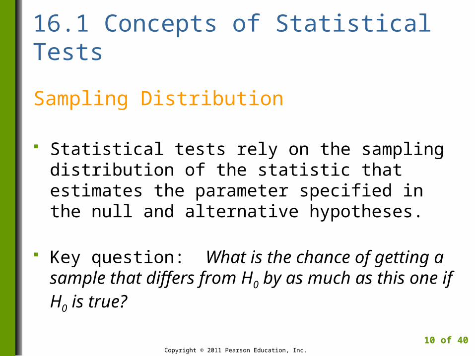
16.1 Concepts of Statistical Tests
Sampling Distribution
Statistical tests rely on the sampling distribution of the statistic that estimates the parameter specified in the null and alternative hypotheses.
Key question: What is the chance of getting a sample that differs from H0 by as much as this one if H0 is true?
Copyright © 2011 Pearson Education, Inc.
10 of 40

16.2 Testing the Proportion
SPAM Software Example
Based on n = 100, = 0.11.
Assuming H0 is true, the sampling distribution of
is approximately normal with mean p = 0.20 and SE( ) = 0.04 (note that the hypothesized value p0 = 0.20 is used to calculate SE).
Copyright © 2011 Pearson Education, Inc.
11 of 40
p̂
p̂p̂

16.2 Testing the Proportion
SPAM Software ExampleWhat is the chance of making a Type I error?
Possible sampling distributions for .Chance of a Type I error shown in shaded area.
Copyright © 2011 Pearson Education, Inc.
12 of 40
p̂

16.2 Testing the Proportion
z–Test and p-Value
p-Value: the largest chance of a Type I error if H0
is rejected based on the observed test statistic.
z-Test: test of H0 based on a count of the standard errors separating H0 from the test statistic.
Copyright © 2011 Pearson Education, Inc.
13 of 40

16.2 Testing the Proportion
z–Test for SPAM Software Example
= -2.25
Copyright © 2011 Pearson Education, Inc.
14 of 40
npp
ppz
/)1(
ˆ
00
0
100/)20.01(20.0
20.011.0
z
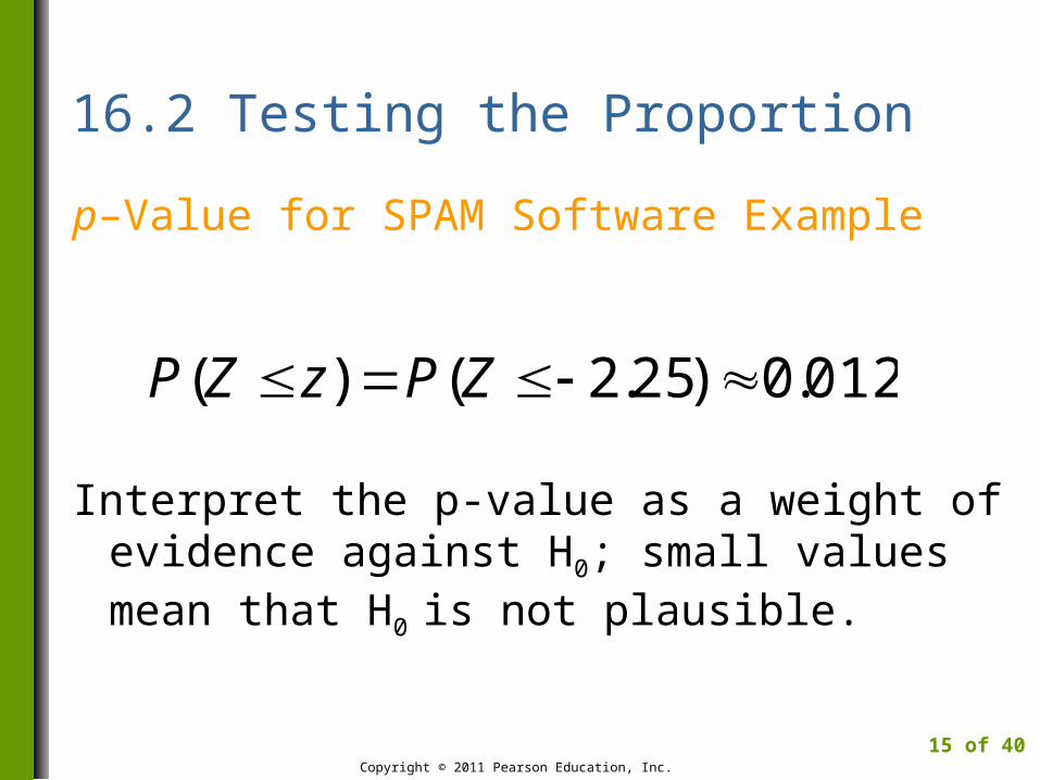
16.2 Testing the Proportion
p–Value for SPAM Software Example
Interpret the p-value as a weight of evidence against H0; small values mean that H0 is not plausible.
Copyright © 2011 Pearson Education, Inc.
15 of 40
012.0)25.2()( ZPzZP
16.2 Testing the Proportion
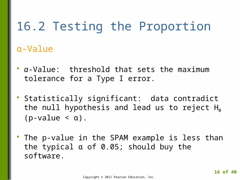
α-Value
α-Value: threshold that sets the maximum tolerance for a Type I error.
Statistically significant: data contradict the null hypothesis and lead us to reject H0 (p-value < α).
The p-value in the SPAM example is less than the typical α of 0.05; should buy the software.
Copyright © 2011 Pearson Education, Inc.
16 of 40
16.2 Testing the Proportion
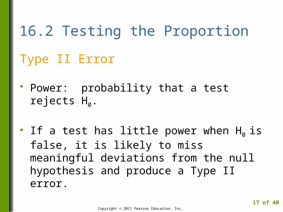
Type II Error
Power: probability that a test rejects H0.
If a test has little power when H0 is false, it is likely to miss meaningful deviations from the null hypothesis and produce a Type II error.
Copyright © 2011 Pearson Education, Inc.
17 of 40

16.2 Testing the Proportion
Summary
Copyright © 2011 Pearson Education, Inc.
18 of 40
16.2 Testing the Proportion
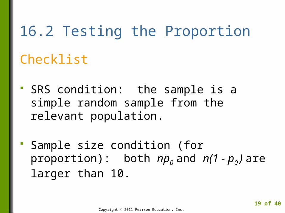
Checklist
SRS condition: the sample is a simple random sample from the relevant population.
Sample size condition (for proportion): both np0 and n(1 - p0 ) are larger than 10.
Copyright © 2011 Pearson Education, Inc.
19 of 40

4M Example 16.1: DO ENOUGH HOUSEHOLDS WATCH?
Motivation
The Burger King ad featuring Coq Roq won critical acclaim. In a sample of 2,500 homes, MediaCheck found that only 6% saw the ad. An ad must be viewed by 5% or more of households to be effective. Based on these sample results, should the local sponsor run this ad?
Copyright © 2011 Pearson Education, Inc.
20 of 40
4M Example 16.1: DO ENOUGH HOUSEHOLDS WATCH?
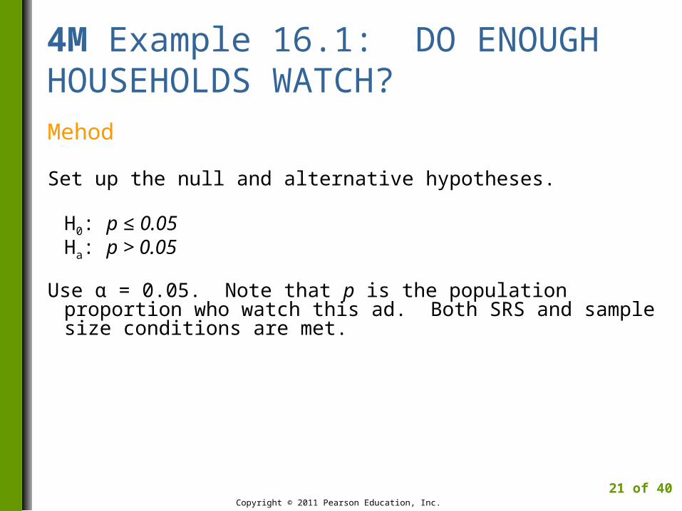
Mehod
Set up the null and alternative hypotheses.
H0: p ≤ 0.05Ha: p > 0.05
Use α = 0.05. Note that p is the population proportion who watch this ad. Both SRS and sample size conditions are met.
Copyright © 2011 Pearson Education, Inc.
21 of 40
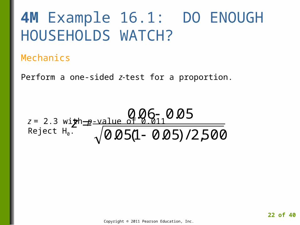
4M Example 16.1: DO ENOUGH HOUSEHOLDS WATCH?Mechanics
Perform a one-sided z-test for a proportion.
z = 2.3 with p-value of 0.011Reject H0.
Copyright © 2011 Pearson Education, Inc.
22 of 40
500,2/)05.01(05.0
05.006.0
z

4M Example 16.1: DO ENOUGH HOUSEHOLDS WATCH?
Message
The results are statistically significant. We can conclude that more than 5% of households watch this ad. The Burger King Coq Roq ad is cost effective and should be run.
Copyright © 2011 Pearson Education, Inc.
23 of 40

16.3 Testing the Mean
Similar to Tests of Proportions
The hypothesis test of µ replaces with .
Unlike the test of proportions, σ is not specified. Use s from the sample as an estimate of σ to calculate the estimated standard error of .
Copyright © 2011 Pearson Education, Inc.
24 of 40
p̂ X
X
16.3 Testing the Mean
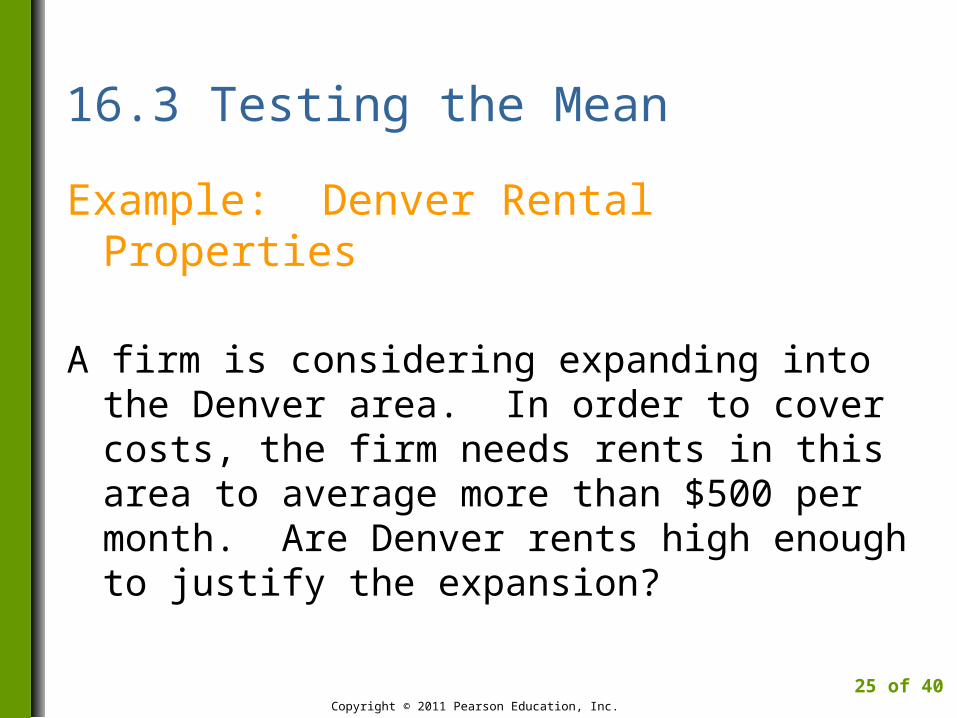
Example: Denver Rental Properties
A firm is considering expanding into the Denver area. In order to cover costs, the firm needs rents in this area to average more than $500 per month. Are Denver rents high enough to justify the expansion?
Copyright © 2011 Pearson Education, Inc.
25 of 40

16.3 Testing the Mean
Null and Alternative Hypotheses
Let µ = mean monthly rent for all rental properties in the Denver area
Set up hypotheses as:H0: µ ≤ µ0 = $500
Ha: µ > µ0 = $500
Copyright © 2011 Pearson Education, Inc.
26 of 40

16.3 Testing the Mean
t - Statistic
Used in the t-test for µ (since s estimates σ)
The t-statistic, with n-1 df, is
Copyright © 2011 Pearson Education, Inc.
27 of 40
ns
xt
/
0

16.3 Testing the Mean
Example: Denver Rental Properties
The firm obtained rents for a sample of size n=45; the average rent was $647 with s = $299.
t = 3.298 with 44 df; p-value = 0.00097Reject H0 ; mean rent exceeds break-even value.
Copyright © 2011 Pearson Education, Inc.
28 of 40
45/299
500647 t

16.3 Testing the Mean
Finding the p-Value in the t-Table
t = 3.298 is larger than any value in the row
Copyright © 2011 Pearson Education, Inc.
29 of 40

16.3 Testing the Mean
Summary
Copyright © 2011 Pearson Education, Inc.
30 of 40

16.3 Testing the Mean
Checklist
SRS condition: the sample is a simple random sample from the relevant population.
Sample size condition. Unless the population is normally distributed, a normal model can be used to approximate the sampling distribution of if n is larger than 10 times both the squared skewness and absolute value of kurtosis.
Copyright © 2011 Pearson Education, Inc.
31 of 40
X

4M Example 16.2: COMPARING RETURNS ON INVESTMENTS
Motivation
Does stock in IBM return more, on average, than T-Bills? From 1980 through 2005, T-Bills returned 5% each month.
Copyright © 2011 Pearson Education, Inc.
32 of 40

4M Example 16.2: COMPARING RETURNS ON INVESTMENTS
Method
Let µ = mean of all future monthly returns for IBM stock. Set up the hypotheses as
H0: µ ≤ 0.005Ha: µ > 0.005
Sample consists of monthly returns on IBM for 312 months (January 1980 – December 2005)
Copyright © 2011 Pearson Education, Inc.
33 of 40

4M Example 16.2: COMPARING RETURNS ON INVESTMENTSMechanics
Sample yields = 0.0106 with s = 0.0805.
t = 1.22 with 311 df; p-value = 0.111
Copyright © 2011 Pearson Education, Inc.
34 of 40
x
ns
xt
/
0
312/0805.0
0050.00106.0 t

4M Example 16.2: COMPARING RETURNS ON INVESTMENTS
Message
Monthly IBM returns from 1980 through 2005 do not bring statistically significantly higher earnings than comparable investments in US Treasury Bills during this period.
Copyright © 2011 Pearson Education, Inc.
35 of 40
16.4 Other Properties of Tests
Significance versus Importance
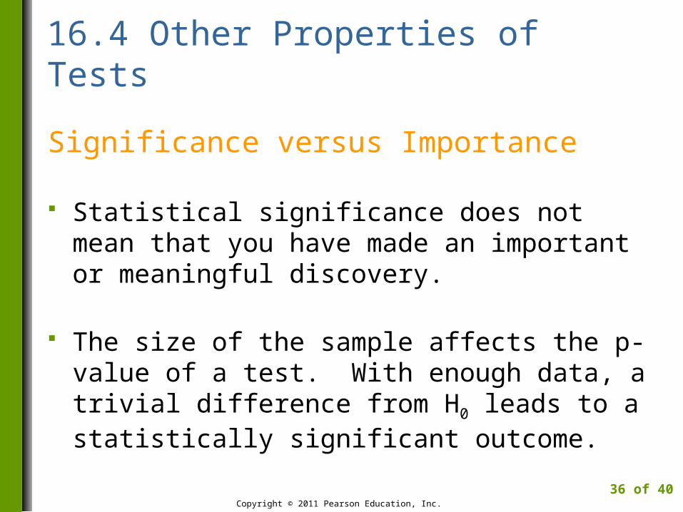
Statistical significance does not mean that you have made an important or meaningful discovery.
The size of the sample affects the p-value of a test. With enough data, a trivial difference from H0 leads to a statistically significant outcome.
Copyright © 2011 Pearson Education, Inc.
36 of 40

16.4 Other Properties of Tests
Confidence Interval or Test?
A confidence interval provides a range of parameter values that are compatible with the observed data.
A test provides a precise analysis of a specific hypothesized value for a parameter.
Copyright © 2011 Pearson Education, Inc.
37 of 40

Best Practices
Pick the hypotheses before looking at the data.
Choose the null hypothesis on the basis of profitability.
Pick the α level first, taking into account both types of error.
Think about whether α = 0.05 is appropriate for each test.
Copyright © 2011 Pearson Education, Inc.
38 of 40

Best Practices (Continued)
Make sure to have an SRS from the right population.
Use a one-sided test.
Report a p–value to summarize the outcome of a test.
Copyright © 2011 Pearson Education, Inc.
39 of 40

Pitfalls
Do not confuse statistical significance with substantive importance.
Do not think that the p–value is the probability that the null hypothesis is true.
Avoid cluttering a test summary with jargon.
Copyright © 2011 Pearson Education, Inc.
40 of 40