copyright © 2014, 2011 pearson education, inc. 1 chapter 27 time series
TRANSCRIPT

Copyright © 2014, 2011 Pearson Education, Inc. 1
Chapter 27Time Series

Copyright © 2014, 2011 Pearson Education, Inc. 2
27.1 Decomposing a Time Series
Based on monthly shipments of computers and electronics in the US from 1992 through 2011, what would you forecast for the future?
Use methods for modeling time series, including regression.
Remember that forecasts are always extrapolations in time.

Copyright © 2014, 2011 Pearson Education, Inc. 3
27.1 Decomposing a Time Series
The analysis of a time series begins with a timeplot, such as that of monthly shipments of computers and electronics shown below.

Copyright © 2014, 2011 Pearson Education, Inc. 4
27.1 Decomposing a Time Series
Forecast: a prediction of a future value of a time series that extrapolates historical patterns.
Components of a time series are:
Trend: smooth, slow meandering pattern. Seasonal: cyclical oscillations related to
seasons. Irregular: random variation.

Copyright © 2014, 2011 Pearson Education, Inc. 5
27.1 Decomposing a Time Series
Smoothing
Smoothing: removing irregular and seasonal components of a time series to enhance the visibility of the trend.
Moving average: a weighted average of adjacent values of a time series; the more terms that are averaged, the smoother the estimate of the trend.

Copyright © 2014, 2011 Pearson Education, Inc. 6
27.1 Decomposing a Time Series
Smoothing: Monthly Shipments Example
Red: 13 month moving average

Copyright © 2014, 2011 Pearson Education, Inc. 7
27.1 Decomposing a Time Series
Smoothing
Seasonally adjusted: removing the seasonal component of a time series.
Many government reported series are seasonally adjusted, for example, unemployment rates.

Copyright © 2014, 2011 Pearson Education, Inc. 8
27.1 Decomposing a Time Series
Smoothing: Monthly Shipments Example
Strong seasonal component (three-month cycle).

Copyright © 2014, 2011 Pearson Education, Inc. 9
27.1 Decomposing a Time Series
Exponential Smoothing
Exponentially weighted moving average (EWMA): a weighted average of past observations with geometrically declining weights.
EWMA can be written as . Hence, the current smoothed value is the weighted average of the current observation and the prior smoothed value.
1)1( ttt wSYwS

Copyright © 2014, 2011 Pearson Education, Inc. 10
27.1 Decomposing a Time Series
Exponential Smoothing
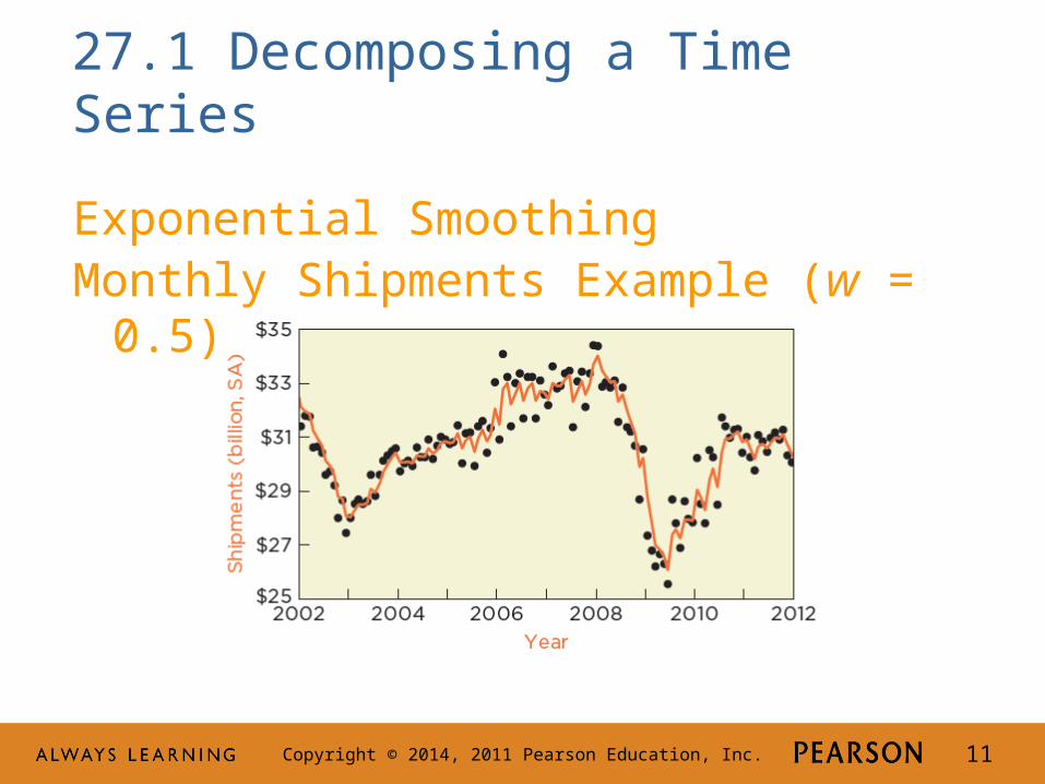
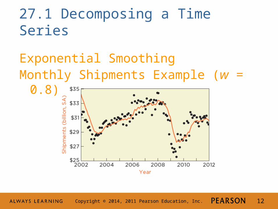
The choice of w affects the level of smoothing. The larger w is, the smoother st becomes.
The larger w is, the more the smoothed values trail behind the observations.
Copyright © 2014, 2011 Pearson Education, Inc. 11
27.1 Decomposing a Time Series
Exponential SmoothingMonthly Shipments Example (w = 0.5)
Copyright © 2014, 2011 Pearson Education, Inc. 12
27.1 Decomposing a Time Series
Exponential SmoothingMonthly Shipments Example (w = 0.8)

Copyright © 2014, 2011 Pearson Education, Inc. 13
27.2 Regression Models
Leading indicator: an explanatory variable that anticipates coming changes in a time series.
Leading indicators are hard to find.
Predictor: an ad hoc explanatory variable in a regression model used to forecast a time series (e.g., time index, t)

Copyright © 2014, 2011 Pearson Education, Inc. 14
27.2 Regression Models
Polynomial Trends
Polynomial trend: a regression model for a time series that uses powers of t as explanatory variables.
Example: the third-degree or cubic polynomial.
tt tttY 33
2210

Copyright © 2014, 2011 Pearson Education, Inc. 15
27.2 Regression Models
Polynomial TrendsMonthly shipments: Six-degree polynomial
The high R2 indicates a great fit to historical data.

Copyright © 2014, 2011 Pearson Education, Inc. 16
27.2 Regression Models
Polynomial TrendsMonthly shipments: Six-degree polynomial
The model has serious problems forecasting.

Copyright © 2014, 2011 Pearson Education, Inc. 17
27.2 Regression Models
Polynomial Trends
Avoid forecasting with polynomials that have high powers of the time index.

Copyright © 2014, 2011 Pearson Education, Inc. 18
4M Example 27.1: PREDICTING SALES OF NEW CARS
Motivation
The U.S. auto industry neared collapse in 2008-2009. How badly did the recession hit this industry?
What would we have expected had the recession not happened?

Copyright © 2014, 2011 Pearson Education, Inc. 19
4M Example 27.1: PREDICTING SALES OF NEW CARS
Motivation – Timeplot of quarterly sales (in thousands)
Cars in blue; light trucks in orange.

Copyright © 2014, 2011 Pearson Education, Inc. 20
4M Example 27.1: PREDICTING SALES OF NEW CARSMethod
Use regression to model the trend and seasonal components apparent in the timeplot. Use a polynomial for trend and three dummy variables for the four quarters.
Let Q1 = 1 if quarter 1, 0 otherwise; Q2 = 1 if quarter 2, 0 otherwise; Q3 = 1 if quarter 3, 0 otherwise.
The fourth quarter is the baseline category. Consider the possibility of lurking variables (e.g., gasoline prices).

Copyright © 2014, 2011 Pearson Education, Inc. 21
4M Example 27.1: PREDICTING SALES OF NEW CARS
MechanicsLinear and quadratic trend fit to the data.
Linear appears more appropriate.

Copyright © 2014, 2011 Pearson Education, Inc. 22
4M Example 27.1: PREDICTING SALES OF NEW CARS
MechanicsEstimate the model.
Check conditions before proceeding with inference.

Copyright © 2014, 2011 Pearson Education, Inc. 23
4M Example 27.1: PREDICTING SALES OF NEW CARSMechanicsExamine residual plot.
This plot, along with the Durbin-Watson statistic D = 0.86, indicates dependence in the residuals.Cannot form confidence or prediction intervals.

Copyright © 2014, 2011 Pearson Education, Inc. 24
4M Example 27.1: PREDICTING SALES OF NEW CARS
Message
A regression model with linear time trend and seasonal factors closely predicts sales of new cars in the first two quarters of 2008, but substantially over predicts sales in the last two quarters and into 2009. The forecasts for 2008 are 1,807 thousand for the first quarter, 2,129 thousand for the second quarter, 1,969 thousand for the third quarter, and 1,741 thousand for the fourth quarter.

Copyright © 2014, 2011 Pearson Education, Inc. 25
4M Example 27.1: PREDICTING SALES OF NEW CARS
Message
Actual values in blue, historical forecasts in orange. Even though the recession ended June 2009, car sales remain less than historical trend.

Copyright © 2014, 2011 Pearson Education, Inc. 26
27.2 Regression Models
Autoregression
Autoregression: a regression that uses prior values of the response as predictors.
Lagged variable: a prior value of the response in a time series.

Copyright © 2014, 2011 Pearson Education, Inc. 27
27.2 Regression Models
Autoregression
Simplest is a simple regression that has one lag:
This model is called a first-order autoregression, denoted as AR(1).
ttt YY 110

Copyright © 2014, 2011 Pearson Education, Inc. 28
27.2 Regression Models
Autoregression Example: AR(1) for Monthly Shipments

Copyright © 2014, 2011 Pearson Education, Inc. 29
27.2 Regression Models
AutoregressionScatterplot of Shipments on the Lag
Indicates a strong positive linear association.

Copyright © 2014, 2011 Pearson Education, Inc. 30
27.2 Regression Models
AutoregressionSummary of AR(1) model for Shipments

Copyright © 2014, 2011 Pearson Education, Inc. 31
27.2 Regression Models
Forecasting an Autoregression
Example: Use AR(1) to forecast shipments.
For Jan. 2010, use observed shipment for Dec. 2009:
1856.0358.4ˆ tt yy
billionyJan 184.28$ˆ 2010.

Copyright © 2014, 2011 Pearson Education, Inc. 32
27.2 Regression Models
Forecasting an Autoregression
For Feb. 2010, there is no observed shipment for Jan. 2010. Use forecast for Jan. 2010:
Once forecasts are used in place of observations, the uncertainty compounds and is hard to quantify.
billionyFeb 484.28$)184.28(856.0358.4ˆ 2010.

Copyright © 2014, 2011 Pearson Education, Inc. 33
27.2 Regression Models
AR(5) Model for Shipments
Fit, forecasts and prediction intervals.

Copyright © 2014, 2011 Pearson Education, Inc. 34
27.3 Checking the Model
Autoregression and the Durbin-Watson StatisticExample 27.1: New Car Sales

Copyright © 2014, 2011 Pearson Education, Inc. 35
27.3 Checking the Model
Autoregression and the Durbin-Watson StatisticExample 27.1: New Car Sales
Copyright © 2014, 2011 Pearson Education, Inc. 36
27.3 Checking the Model
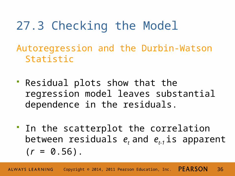
Autoregression and the Durbin-Watson Statistic
Residual plots show that the regression model leaves substantial dependence in the residuals.
In the scatterplot the correlation between residuals et and et-1 is apparent (r = 0.56).

Copyright © 2014, 2011 Pearson Education, Inc. 37
27.3 Checking the Model
Autoregression and the Durbin-Watson Statistic
The Durbin-Watson statistic is related to the autocorrelation of the residuals in a regression:
)1(2)(
1
1
2
2
21
re
eeD n
ii
n
itt

Copyright © 2014, 2011 Pearson Education, Inc. 38
27.3 Checking the Model
Summary
Examine these plots of residuals when fitting a time series regression:
Timeplot of residuals; Scatterplot of residuals versus fitted values; and Scatterplot of residuals versus lags of the
residuals.

Copyright © 2014, 2011 Pearson Education, Inc. 39
4M Example 27.2: FORECASTING UNEMPLOYMENT
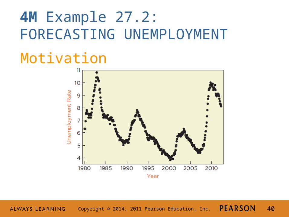
Motivation
Using seasonally adjusted unemployment data from 1980 through the end of 2011, can a time series regression predict what happens to unemployment in 2012?
Copyright © 2014, 2011 Pearson Education, Inc. 40
4M Example 27.2: FORECASTING UNEMPLOYMENT
Motivation

Copyright © 2014, 2011 Pearson Education, Inc. 41
4M Example 27.2: FORECASTING UNEMPLOYMENT
Method
Use a multiple regression of the percentage unemployed on lags of unemployment and time trends. In other words, use a combination of an autoregression with a polynomial trend.
The scatterplot matrix shows linear association and possible collinearity; hopefully the lags will capture the effects of important omitted variables.

Copyright © 2014, 2011 Pearson Education, Inc. 42
4M Example 27.2: FORECASTING UNEMPLOYMENT
MechanicsEstimate the model.

Copyright © 2014, 2011 Pearson Education, Inc. 43
4M Example 27.2: FORECASTING UNEMPLOYMENT
Mechanics
All conditions for the model are satisfied; proceed with inference.
Based on the F-statistic, reject H0. The model explains statistically significant variation. The fitted equation is
)(131.0988.0079.0ˆ 611 tttt yyyy

Copyright © 2014, 2011 Pearson Education, Inc. 44
4M Example 27.2: FORECASTING UNEMPLOYMENT
Message
A multiple regression fit to monthly unemployment data from 1980 through 2011 predicts that unemployment in January 2012 will be between 8.1 and 8.7% with 95% probability. Forecasts for February and March call for unemployment to fall further to 8.3% and 8.2%, respectively.

Copyright © 2014, 2011 Pearson Education, Inc. 45
4M Example 27.3: FORECASTING PROFITS
Motivation
Forecast Best Buy’s gross profits for 2012. Use their quarterly gross profits from 1995 to 2011.

Copyright © 2014, 2011 Pearson Education, Inc. 46
4M Example 27.3: FORECASTING PROFITS
Method
Best Buy’s profits have not only grown nonlinearly (faster and faster), but the growth is seasonal. In addition, the variation in profits appears to be increasing with level. Consequently, transform the data by calculating the percentage change from year to year. Let yi denote these year-over-year percentage changes.

Copyright © 2014, 2011 Pearson Education, Inc. 47
4M Example 27.3: FORECASTING PROFITS
MethodTimeplot of year-over-year percentage change.

Copyright © 2014, 2011 Pearson Education, Inc. 48
4M Example 27.3: FORECASTING PROFITS
MethodScatterplot of the year-over-year percentage change on its lag.
Indicates positive linear association.

Copyright © 2014, 2011 Pearson Education, Inc. 49
4M Example 27.3: FORECASTING PROFITS
MechanicsEstimate the model.

Copyright © 2014, 2011 Pearson Education, Inc. 50
4M Example 27.3: FORECASTING PROFITS
Mechanics
All conditions for the model are satisfied; proceed with inference.
The fitted equation has R2 = 74.5% with se = 6.99.
The F-statistic shows that the model is statistically significant. Individual t-statistics show that each slope is statistically significant.
Copyright © 2014, 2011 Pearson Education, Inc. 51
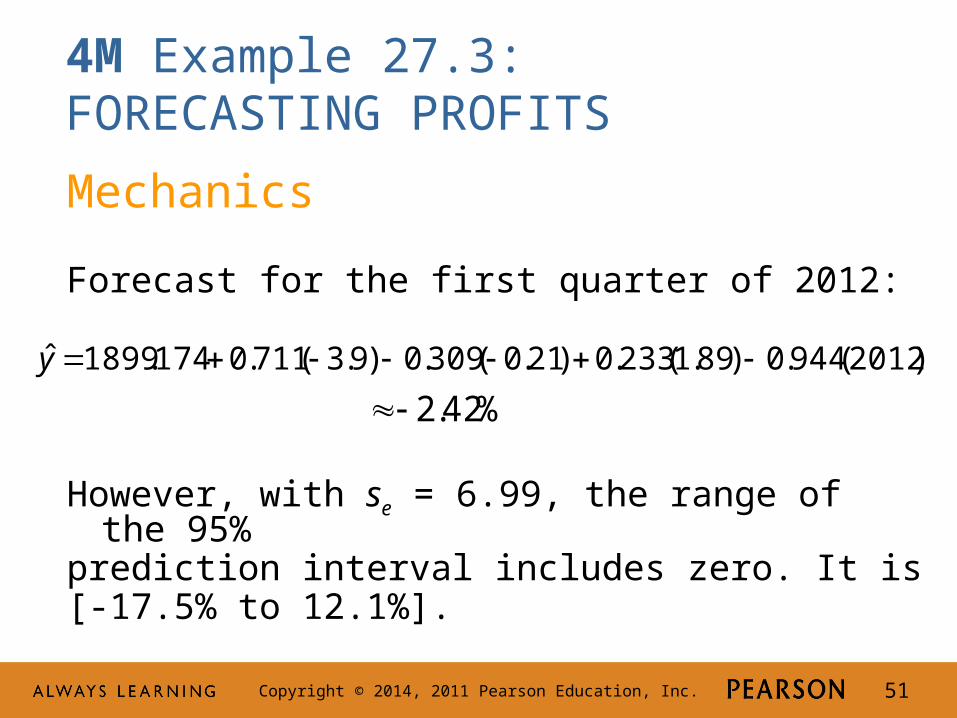
4M Example 27.3: FORECASTING PROFITS
Mechanics
Forecast for the first quarter of 2012:
However, with se = 6.99, the range of the 95% prediction interval includes zero. It is [-17.5% to 12.1%].
)2012(944.0)89.1(233.0)21.0(309.0)9.3(711.0174.1899ˆ y
%42.2

Copyright © 2014, 2011 Pearson Education, Inc. 52
4M Example 27.3: FORECASTING PROFITS
Message
The time series regression that describes year-over-year percentage changes in gross profits at Best Buy is significant and explains 75% of the historical variation. It predicts profits in the first quarter of 2012 to fall about 2.4% below profits in the first quarter of 2011; however, the model can’t rule out an increase (up to 12%) or substantial contraction (dropping about 17%).

Copyright © 2014, 2011 Pearson Education, Inc. 53
Best Practices
Provide a prediction interval for your forecast.
Find a leading indicator.
Use lags in plots so that you can see the autocorrelation.

Copyright © 2014, 2011 Pearson Education, Inc. 54
Best Practices (Continued)
Provide a reasonable planning horizon.
Enjoy finding dependence in the residuals of a model.
Check plots of residuals.

Copyright © 2014, 2011 Pearson Education, Inc. 55
Pitfalls
Don’t summarize a time series with a histogram unless you’re confident that the data don’t have a pattern.
Avoid polynomials with high powers.
Do not let the high R2 of a time series regression convince you that predictions from the regression will be accurate.

Copyright © 2014, 2011 Pearson Education, Inc. 56
Pitfalls (Continued)
Do not include explanatory variables that also have to be forecast.
Don’t assume that more data is better.