copyright 2015, lakshmi sindhuri juturu
TRANSCRIPT

Applying Big Data Analytics on Integrated Cybersecurity Datasets
by
Lakshmi Sindhuri Juturu, B.Tech
A Thesis
In
Computer Science
Submitted to the Graduate Faculty
of Texas Tech University in
Partial Fulfillment of
the Requirements for
the Degree of
Master of Sciences
Approved
Dr. Susan D. Urban
Co-chair of Committee
Dr. Yong Chen
Co-chair of Committee
Mark Sheridan
Dean of the Graduate School
May, 2015

Copyright 2015, Lakshmi Sindhuri Juturu

Texas Tech University, Lakshmi Sindhuri Juturu, May 2015
ii
ACKNOWLEDGMENTS
I would like to express my deepest gratitude to my advisor, Dr. Susan D.
Urban, for her untiring support, persistent guidance, and encouragement without
which this work would not have been possible. I owe her, more than what I can
mention, for giving me the opportunity to work under her valuable supervision. This
experience has been enriching for me to grow professionally and personally, and
helped me become a better person. I gained technical and functional knowledge, and
inter-personal skills which will stay with me throughout my life. The freedom she
gave me is the key factor behind the success of this work.
I would also like to thank my co-advisor and committee member, Dr. Yong
Chen, for his timely help, support, and advice. I can't thank him enough for always
ensuring that my journey throughout the thesis is hassle-free.
I would like to thank my parents, JVNS Prasada Rao and Narayani; my sister,
Raga Madhuri; my husband, Harshvardhan Gazula; and my grandparents. Without
their patience, guidance, understanding, support, and most of all unconditional love
and care, I wouldn’t be what I am today.
I would like to thank my colleagues and very special friends Mr. Narasimha
Inukollu and Ms. Kalaranjani Vijayakumar for supporting me all the time and assuring
me throughout. Without their help and suggestions, I would not be able to put all the
things together in place.

Texas Tech University, Lakshmi Sindhuri Juturu, May 2015
iii
TABLE OF CONTENTS
ACKNOWLEDGMENTS .................................................................................... ii
ABSTRACT .......................................................................................................... iv
LIST OF TABLES ................................................................................................ v
LIST OF FIGURES ............................................................................................. vi
I. INTRODUCTION ............................................................................................. 1
II. RELATED WORK .......................................................................................... 7
Background on Cybersecurity and Big Data Computing .................................. 7
HBase Schema Design Issues for Storing Datasets ........................................ 10
Tools and Methods for Anomaly Detection using HBase .............................. 12
Data Mining and Machine Learning Approaches ........................................... 15
III. SELECTION AND PREPARATION OF CYBERSECURITY
DATASETS .......................................................................................................... 21
IV. HBASE DESIGN ALTERNATIVES FOR STORING DATASETS ....... 27
Use Case Requirements .................................................................................. 27
Design Alternatives ......................................................................................... 28
Design Evaluation ........................................................................................... 32
V. DATA MINING AND MACHINE LEARNING APPLIED TO
CYBERSECURITY DATASETS ...................................................................... 37
Use of Logistic Regression ............................................................................. 37
Use of Fuzzy k-Means .................................................................................... 44
Comparison and Analysis of LR and FKM Algorithms ................................. 49
VI. CONCLUSION AND FUTURE WORK .................................................... 51
Conclusion ...................................................................................................... 51
Future Work .................................................................................................... 51
BIBLIOGRAPHY ............................................................................................... 53

Texas Tech University, Lakshmi Sindhuri Juturu, May 2015
iv
ABSTRACT
With the growing prevalence of cyber threats in the world, various security
monitoring systems are being employed to protect the network and resources from the
cyber attacks. The large network datasets that are generated in this process by security
monitoring systems need an efficient design for integrating and processing them at a
faster rate. In this research, a storage design scheme has been developed using HBase
and Hadoop that can efficiently integrate, store, and retrieve security-related datasets.
The design scheme is a value-based data integration approach, where data is integrated
by columns instead of by rows. Since rowkeys are the most important aspect of HBase
table design and performance, a rowkey design was chosen based on the most
frequently accessed columns associated with use cases for the retrieval of the dataset
statistics. Tests conducted on various schema design alternatives prove that the rate at
which the datasets are stored and retrieved using the model designed as part of this
research is higher than that of the standard method of storing data in HBase.
Network datasets representing DDoS attacks have been used for integration in
this research. Use case requirements have been identified, which are related to the
characteristics of attacker IP addresses from the integrated datasets, to generate
statistical data. This statistical data was used to run the Logistic Regression (LR)
classification algorithm for classifying the network traffic data into attack-related and
non-attack related traffic. The Fuzzy k-Means (FKM) algorithm was also used to
create clusters of attackers and non-attacks to segregate the attack-related traffic from
the network datasets. The results obtained from the two algorithms show that both LR
and FKM algorithms can successfully classify the network traffic datasets into
attackers and non-attackers.

Texas Tech University, Lakshmi Sindhuri Juturu, May 2015
v
LIST OF TABLES
3.1 Sample table structure of ‘from-victim’ dataset converted in .csv format 24
4.1 Test results of loading and running one use case on a single DDoS
attack data file using Hadoop Cluster ........................................... 33
5.1 Sample values (poor results) of the model generated using a
single dataset ................................................................................. 41
5.2 Snapshot of the input dataset prepared for LR algorithm ......................... 42
5.3 Sample values of the model generated using incremented
variables and datasets .................................................................... 43
5.4 Sample values of the model evaluated on the complete input
datasets .......................................................................................... 44

Texas Tech University, Lakshmi Sindhuri Juturu, May 2015
vi
LIST OF FIGURES
3.1 Snapshot of the DDoS attack dataset accessed through
Wireshark ...................................................................................... 22
3.2 Cross-mapping of Source and Destination columns of from-
victim and to-victim files .............................................................. 25
4.1 Method of storing datasets in rows table followed by field tables ............ 29
4.2 Architectural design to identify attackers from network traffic ................ 32
4.3 Avg. use case runtimes of individual passes for each schema
design ............................................................................................ 33
4.4 Time taken to load datasets in HVID and HBaseSchema models ............ 34
4.5 Avg. time taken to run use cases in Standard HBase, HVID and
HBaseSchema models ................................................................... 36
4.6 The three clusters formed using FKM algorithm ...................................... 49

Texas Tech University, Lakshmi Sindhuri Juturu, May 2015
1
CHAPTER I
INTRODUCTION
With the advent of big data technology, many industrial problems and
challenges that are related to large volumes of data are now being addressed. Many
industries and companies are able to analyze and process volumes of data which was
once beyond their capability. While many domains have benefited through the use of
big data technologies, cybersecurity is one field that is just beginning to explore the
advantages of big data analytics. The ability to detect and stop cyber attacks can make
or break an enterprise (Harper, 2013). By means of big data, organizations may be
able to rigorously detect threats, create more defense mechanisms and improve
security.
Prior to the arrival of big data storage, most security systems have been
dedicated to a single type of threat detection. SIEM (Security Information and Event
Management) systems (Cardenas et al., 2013) do exist that are capable of analyzing
data from several log files, but such systems are limited to the amount of data they can
handle. With systems such as Hadoop (Hadoop, 2005), cybersecurity data can now be
stored in a dedicated repository which can not only accommodate more than three
months of data but also combine and analyze real-time data together with historical
data. Big data analytics can be run on long-term patterns and detect advanced
persistent threats (APTs) that become manifest over time.
Big data analytics play an important role in detecting advanced threats and
insider threats (Gartner, 2014). Monitoring systems can potentially minimize false
alarms by providing smarter analytics. Data analytics can be used to assist systems in
collecting internal data by merging with relevant external data to detect known
patterns to stay ahead of malicious activities or intruders. Currently, 8% of major
global companies (Gartner, 2014) have adopted big data analytics for one or more use
cases related to security and fraud detection. Gartner predicted that within a year, this
will be increased to 25% with a positive return on investment within six months of
implementation. Data analysis should be intelligent and timely as anything that is

Texas Tech University, Lakshmi Sindhuri Juturu, May 2015
2
delayed will lose its value, especially in the field of cybersecurity. Given that hackers
are well aware of security measures and other fraud detection measures that are
employed by enterprises, they are able to directly attack without any reconnaissance
phase. Hence, to be always a step ahead, enterprises can use big data analytics to
improve monitoring systems and detection systems with contextual data and apply
smarter analytics. Data correlation techniques can be used among the high-priority
alerts and monitoring systems to detect patterns and get a bigger picture on the state of
security. Also, enterprises can opt for fast tuning of their rules and models to test
against data streaming close to real time.
The Teradata report (Ponemon, 2013) states that the traditional methods that
fall short in detecting and preventing threats can be enhanced with big data analytics.
Many big data tools and techniques have emerged that can efficiently handle the
volume and complexity of varied kinds of data, such as machine-generated and
network-related data. Also, the results from the survey conducted by Teradata
indicate, that the shortcomings of traditional solutions in detecting and preventing
threats can be overcome by using big data analytics. Hence, big data systems are being
part of a cyber defense strategy for every enterprise to meet the needs of complex and
large-scale analytics.
A concern with the cybersecurity monitoring process is that when multiple
security monitoring systems are employed and each system generates numerous log
files (such as security logs, network traffic logs), there is no well-established system
that can identify the relationships among these log files and integrate them. These
related log files could potentially be useful for identifying attack related patterns that
help in early detection of APTs or any malicious attacks. The work in (Labrinidis,
2012) identifies the challenges in dealing with big data analysis, such as automating
the whole process of locating, identifying and understanding the data. A suitable
database design is required even when analyzing one single dataset. Similarly, mining
requires data to be integrated, cleaned and efficiently accessible, which involves the
use of effective mining algorithms and big data computing environments. Labrinidis
(Labrinidis, 2012) also describes that significant research is required in order to

Texas Tech University, Lakshmi Sindhuri Juturu, May 2015
3
achieve automated integration of data sets as well as a suitable database design, even
for simpler analysis of a single data set. It is also essential that effective mining
techniques are used to extract information from the large datasets.
The objective of this research is to investigate the manner in which a system
such as HBase (HBase, 2006) can be used to support the integration and mining of
security-related datasets. In particular, this research aims to 1) create a design for the
integration of cybersecurity datasets in a system developed using Hadoop and HBase,
and 2) experiment with data mining or machine learning techniques on the integrated
files, which may potentially help in identifying attack patterns and segregating attack-
related traffic from the normal traffic.
A unique approach is designed using HBase, which can effectively support the
integration of multiple network-related datasets. The approach is based on the initial
work done by Stearns (Stearns, 2014) that describes a value-based data integration
approach, where data is integrated by columns instead of rows. Separate tables are
pooled into a common collection of columns, which can be effectively treated as one
single table possessing all fields. This work is inspired by neural-networks (Nielsen,
2001), which involves inversion of the column-table structure. In this approach, data
from all sources are stored by value instead of by row ID in a column-table where
values are the keys, which are stored as row IDs. Using this approach, tables can be
directly queried for rows by direct lookup of column values without scanning the
entire table. Furthermore, an inner join operation using a shared column among two
different tables can be performed using already collected row IDs and grouping them
as required. Also, data can be quickly merged without having to worry about what
columns are used for merging. MapReduce operations can also be performed easily on
the merged data.
In this research, two network-related data files are integrated by identifying
and mapping the relationships between the files. Other design alternatives are taken
into consideration. Since, rowkeys are the most important aspect of HBase table
design and the performance of data extraction from an HBase table is affected by the
row keys (Khurana, 2012), different rowkeys are considered as per the access patterns
Texas Tech University, Lakshmi Sindhuri Juturu, May 2015
4
required for this work. These data files mainly deal with IP addresses and timestamps.
Hence, potential schema designs are chosen by selecting the most frequently accessed
columns and their combinations as a part of the rowkey and testing performance using
each rowkey. Major use cases such as performing read operations, write operations
and the selection of a particular range of data are tested thoroughly to identify the best
possible schema design that can be attributed to each use case.
For this research, DDoS datasets have been used that are publicly available
from CAIDA (Center for Applied Internet Data Analysis), (The CAIDA, 2007).
CAIDA is a collaborative undertaking among government, research and commercial
organizations to promote research and development in providing robust and secure
internet infrastructure. This organization provides datasets for possible research
purposes while preserving the privacy of individuals and of organizations that donated
the data. It contains datasets obtained from over a decade consisting of various attacks
such as DDoS (DDOS Attack, 2007), the Code-Red virus (Danyliw, 2001), Conficker
(Conficker Worm, 2008), witty worm (Shannon and Moore, 2004), monitored logs
and network traffic datasets. Among these datasets, DDoS attack datasets are of high
focus. The DDoS type of attack attempts to block access to the targeted server by
consuming all the resources on the server and the bandwidth of the network that is
connecting the server to the internet. This DDoS attack dataset contains approximately
one hour of traffic traces that have been anonymized from the original attack. This
entire dataset is divided into individual files each containing five minute intervals of
data in the format of .pcap (packet capture) files.
Once the datasets are successfully integrated, data mining techniques are
applied on the statistical data obtained from the integrated datasets. These analytics
help in identifying the attack related traffic from normal traffic and also to extract
attack patterns. The Fuzzy k-Means (FKM) clustering algorithm and the Logistic
Regression (LR) classification algorithm have been performed on the time-related and
connection-related data obtained from the integrated datasets. Since the DDoS datasets
collected from CAIDA contain purely attack-related data, the files have been merged
with normal network traffic to a desktop in the TTU network that was captured using
Texas Tech University, Lakshmi Sindhuri Juturu, May 2015
5
the Wireshark tool. Individual tests were performed on the attack traffic, normal traffic
and on the combination of both the data files. The FKM algorithm was used to create
attacker and non-attacker clusters. For the LR algorithm, inferences drawn initially are
validated against the existing black listings (malicious information) and white listings
from the DNS lookup as part of a training phase. The model generated using the
sample dataset in the training phase is used for running the testing phase on the actual
dataset. Different models are generated by changing the key parameters and the testing
phase is repeated several times for accuracy and efficiency in results. The results
obtained from both the algorithms have been validated against each other for verifying
the attack-related traffic.
Initially, an HBase storage model designed by Stearns (Stearns, 2014) was
used for storing the DDoS attack datasets that took 304338 ms to load 220k rows of
data and an average time of 4005.7 ms to query the total number of requests made by
each IP address. This model was improved as part of this research with a new schema
design that took 262682 ms to load 220k rows of data and an average time of 3863.1
ms to run the same query. The statistical data retrieved from the improved HBase
model for all the unique IP addresses (Total - 41), was first sent to LR algorithm to
classify the attackers and non-attackers from the data. The LR algorithm accurately
classified 34 IP addresses as attackers and the remaining 7 IP addresses as non-
attackers from the total 41 unique IP addresses. The statistical data was also sent to the
FKM algorithm for creating attacker and non-attacker clusters. The FKM algorithm
created a cluster-1 of 11 attackers, cluster-2 of 21 attackers, and a cluster-3 of 7 non-
attackers, with clusters 2 and 3 sharing 2 attackers, as the FKM algorithm is known for
creating soft clusters. Although, both of the algorithms gave similar results, the LR
algorithm provided a complete and accurate classification identifying attack-related
traffic from the network traffic.
Since different network security systems and tools generate log files in an
individual format and might contain bits and pieces of attack information, it is
beneficial to have an integrated set of data that can be analyzed for attack patterns.
This research demonstrates the integration and analysis of datasets for identifying

Texas Tech University, Lakshmi Sindhuri Juturu, May 2015
6
attack-related traffic that can potentially lead to easier threat detection in cases where
attacks occur on multiple targets.
The remaining chapters of this thesis are organized as follows. Chapter 2
discusses the related work and Chapter 3 explains the selection and preparation of
cybersecurity datasets. Chapter 4 describes the HBase design alternatives that are
considered as part of this work. Chapter 5 presents the findings of the data mining
algorithms that are used on the statistical data generated from the integrated datasets,
while Chapter 6 presents conclusions and future research directions.

Texas Tech University, Lakshmi Sindhuri Juturu, May 2015
7
CHAPTER II
RELATED WORK
This chapter presents the past and current research that is related to this thesis
work. It provides an overview on the 1) background research on cybersecurity and big
datasets, 2) current research work that addresses the HBase design issues for storing
and accessing big data, 3) existing tools and methods that use Hadoop and HBase for
anomaly detection, and 4) data mining and machine learning approaches that have
been used for cybersecurity research.
Background on Cybersecurity and Big Data Computing
Many big data systems are enabling the storage and analysis of large
heterogeneous data sets at exceptional scale and speed (Big Data, 2013). These
systems have the potential to provide significant advancements in security intelligence
by reducing the time taken for data consolidation, contextualization of security event
information, and correlation of historical data for forensic purposes. Initially, data is
collected at a massive scale from many internal and external sources. Then, deeper
analytics are performed on the data by providing a consolidated view of security-
related information. Big data analytics can also be employed to analyze financial
transactions, log files, and network traffic in identifying anomalies, suspicious
activities and fraud detection. In this context, the more data that is collected, the
greater value that can be derived from the data. However, there are several challenges
such as privacy challenges, legal challenges and technical issues regarding data
collection, storage and analysis that developers have to overcome for performing
potential big data analytics.
HP labs has investigated big data analytics for security challenges by
introducing large-scale graph inference and analysis of a large collection of DNS
events, which consists of requests and responses. Large-scale graph inference
identifies malware-infected hosts in a network and maps them with the malicious
domains accessed by those hosts (Big Data, 2013). This information is again validated
using an existing black list and white list to identify the likelihood for the host and

Texas Tech University, Lakshmi Sindhuri Juturu, May 2015
8
domain to be malicious. This experiment was conducted on billions of HTTP requests,
DNS request data and NIDS (Network Intrusion Detection Systems) data sets
collected worldwide and finding that high true positive rates and low false positive
rates are achieved, which can be used to train anomaly detectors. Large collections of
DNS events are used to identify botnets or any kind of malicious activity in the
network by deriving domain names, time stamps, and DNS response time-to-live
values. Classification techniques such as decision trees and support vector machines
were then used to identify infected hosts and malicious domains. Although, the graph
inferences used here are well suited for handling complex types of data, this approach
can use a lot of space and the operations performed on these large amounts of data are
possibly slow (Sherman, 2014). The research presented in this thesis has focused on
integrating datasets through a unique design using HBase instead of using the
traditional way of storing the datasets in HBase. This approach helps in faster retrieval
of data, as anything that is delayed will lose its value, especially in the case of attack
detection.
Big data analytics has the ability to correlate data from a wide range of data
sources across significant time periods. This helps in reducing false alarms and
improving threat detection even when mixed with authorized user activities (Virvilis et
al., 2013). Also, the analytics do not have to be performed in real-time. An
organization can always perform the analysis within an acceptable time and provide
warnings to the security professionals about potential attacks. The work in (Virvilis et
al., 2013) also describes the importance of offline analysis along with the real time
data in threat detection. Although analyzing the offline data causes a delay in the
attack detection, it is equally important to consider the time the attackers spend in
reaching their objective. For instance, after gaining the initial access, attackers take
significant time to explore the network, navigate across subnets and identify their
desired location. These steps are performed as stealthily as possible to avoid any
detection. Here, big data analytics plays a key role in identifying the correlation of
events across large time scales and from multiple sources which are very crucial for
detecting sophisticated attacks. To achieve these needs, big data analytics support

Texas Tech University, Lakshmi Sindhuri Juturu, May 2015
9
dynamic collection, consolidation and correlation of data from diversified data
sources. Unlike SIEM systems, the use of big data technologies does not have any
limitations to perform correlation in a given time window. In fact, it increases the
scope and quantity of data over which correlation can be performed. These data
correlations result in a lower rate of false positives and increase the probability of
detecting the threats.
Although data analytics performed on real-time data is effective against
traditional attacks, most of the unique characteristics of attacks are not addressed.
Hence, the research in this thesis concentrates on processing the datasets that are
previously generated instead of real-time data. Data correlation is performed among
the existing datasets that are related with each other, in order to identify potential
relations between the datasets. For instance, the DDoS datasets used as part of this
research contain a number of files, with each file spanning across five minute
intervals. The statistics that are generated from each file are matched with the
remaining files that are being considered to obtain the correlation among different
events across a large scale. These events constitute the total number of attempts made
by one host to connect to the server in a given time, the number of packets that are
being sent over the network, and its time-to-live factor. Correlation helps in
identifying two or more hosts if they are behaving in a similar way by sending the
same type and number of requests in a given time span. This helps in detecting
malicious hosts that are trying to flood a network or make a server unavailable to
authenticated clients.
Big data analytics still faces a number of practical limitations. Also, a few
questions arise often regarding authenticity and integrity of the data that is being used
for analytics and the challenges in securing the data. Hence, good visualization tools
are needed to help analysts understand the data. Research is also needed to build a
complete solution that significantly enhances the detection capabilities for uncovering
threats and malicious activity. Using open source implementations of big data systems,
mainly Hadoop (Hadoop, 2005), to test the execution of more complex detection
algorithms would be beneficial.

Texas Tech University, Lakshmi Sindhuri Juturu, May 2015
10
HBase Schema Design Issues for Storing Datasets
Open source projects like Hadoop and HBase are common platforms for big
data solutions, where Hadoop is a cross-platform distributed file system that allows
computationally independent systems to process enormous amounts of data (Big Data,
2012). HBase is an open-source, NoSQL, highly-reliable, efficient, row-oriented and
expandable distributed database system. HBase utilizes Hadoop HDFS as its own
storage system and runs Hadoop MapReduce to process huge datasets. It can easily
store large amounts of unstructured data and is great for processing large datasets, as
the Hadoop Distributed File System (HDFS) provides a reliable low-level storage
support for HBase (Zhao et al., 2014).
While HBase provides lot of features and many design choices to the user, the
crucial feature for best performance lies in the schema design. In schema design or
table design, the emphasis is particularly given on rowkey design as the lack of
secondary indexes in HBase forces the use of the rowkey for column name sorting
(George, 2012). Choosing sequential keys for sequential reads are the best but provide
poor performance where writes are concerned. Similarly, random keys are good for
performing writes, but provide poor performance in read operations. Based on the
access pattern, sequential rowkeys, random rowkeys, or even the combination of both
can be chosen. Choosing a good rowkey will improve the read and write performance.
HBase provides many options to choose the rowkey, such as salting, hashing,
randomization and key field swapping techniques, to prevent hot-spotting and other
issues, with each of them having their own pros and cons (HBase, 2006). Hot spotting
is a problem in which most of the clients’ requests are directed to a single node or a
small set of nodes of a large cluster, keeping other nodes idle and wasting its
resources. The problem of hot spotting can be eradicated by distributing the data to
create a well load-balanced cluster that can be achieved by changing the rowkey
design. It is possible that a particular rowkey design which provides best write
performance might give the worst read performance and vice versa. Therefore, it is
necessary to choose good rowkey design based on the requirements.
Texas Tech University, Lakshmi Sindhuri Juturu, May 2015
11
The Salting approach to rowkey design is explained in (HBase, 2006) where
random numbers are generated and each number is appended to the rowkey, which
will help in writing data on multiple regions. Salting provides effective throughput in
performing write operations, but comes with the cost of bad read performance,
especially in scenarios that require reading the data in lexicographic order and reading
all of the different regions. Other approaches to rowkey design include hashing,
appending column names with the row id, and the combination of both. As a result,
there is no particular rowkey design that is suitable for all cases. Rowkey design
depends upon the use case of the client. Major work has been done on designing
rowkeys based on the data and processing requirement (HBase, 2006). For a use case
related to Log Data and Timeseries Data, certain possible rowkey design approaches
are mentioned in (HBase, 2006), with the given columns Hostname, Timestamp, Log
event, Value / Message. All of these column data are stored in an HBase table called
LOG_DATA. The possible rowkey design could be the combination of columns,
hostname, timestamp and log event. The row key combination of [timestamp] [hostname]
[log event] will cause a monotonically increasing rowkey problem (HBase, 2006).
Modifying this approach by adding buckets at the front of the key is another rowkey
design. Timestamps are distributed to different buckets by performing the modulus of
the timestamps with the total number of buckets. This technique is mainly useful for
time-oriented scans, but has a problem for selecting data for a particular range of
timestamp. The rowkey combination as [hostname] [log event] [timestamp] is useful
in the scenario where the search criteria is hostname centric. The rowkey design
[timestamp] or [reverse timestamp] is used to get the most recently captured data
quickly.
Based on this approach, the research of this thesis has tried three possible
combinations of Table Id, Row Id, column name, value and timestamp for designing the
rowkey, monitoring the read and write times for each identified rowkey design.
Among the three choices, the optimal design, which has a rowkey as a value followed
by hash value of Table Id and hash value of Row Id, is chosen for the field tables, and
hash value of Destination column followed by hash value of Time is chosen as the
Texas Tech University, Lakshmi Sindhuri Juturu, May 2015
12
rowkey for row tables. Further details about the rowkey design as well as Field and
row tables are provided in Chapters 3 and 4.
Tools and Methods for Anomaly Detection using HBase
The network data logs that are received from each data source contain different
formats, unless it is employed in the network to generate the data logs from a single
vendor. Since it is an uncommon scenario, these log files that are generated in
different formats, sometimes known as 'dirty data', cannot be easily correlated and
analyzed as a whole. To collect the data from different sources holistically, any service
wishing to use the data needs to examine and restructure each of the disjointed formats
separately to suit its analysis approach (Yen et al., 2013). There are certain tools that
use the SIEM approach for logging and analyzing the data from multiple sources and
efficiently handle the big data sets they generate using their own distributed storage
and processing techniques. However, these tools come at the cost of not being able to
change the security monitoring methods without losing data unification and other
dependency challenges (Big Data, 2013).
To combine multiple network monitoring systems at EMC Corporation, the
Beehive system was designed and implemented to handle the large scale logging data
produced by the systems at EMC (Yen et al., 2013). This system analyzes large
volumes of disparate log data collected in organizations to detect malicious activity,
which includes malware infections and policy violations. As described in (Yen et al.,
2013), there is lot of pre-processing of data that must be done before performing
analysis, such as timestamp normalization among different datasets, IP address-to-host
mappings, and detection of static IP addresses and dedicated hosts. However, there are
certain challenges in the implementation, such as the need for efficient data reduction
algorithms for timely detection of critical threats and strategies to focus on security-
relevant information in the logs.
This thesis has designed a value-based data integration approach, where data is
integrated by columns instead of rows. Separate tables are pooled into a common
collection of columns, which can be effectively treated as one single table possessing
Texas Tech University, Lakshmi Sindhuri Juturu, May 2015
13
all fields. However, to perform the join of different fields by a shared field, it is
necessary to scan the entire table for the values of each field and its corresponding
rows. Hence, a storage approach is developed which is inspired by neural-networks
(Nielsen, 2001) to invert the column-table structure. In this approach, data from all
sources are stored by value instead of by row ID in a column-table, where values are
the keys, which are stored by row IDs. This approach supports the ability to directly
query for rows from any table using direct lookup of a column value without scanning
the entire table. Even an inner join operation by a shared column can be performed
using already collected row IDs and grouping them as required.
The research in (Lee and Lee, 2011) describes a DDoS anomaly detection
method that was developed by implementing a detection algorithm based on Hadoop
and MapReduce. This technique works against the HTTP GET flooding attack.
Counter-based detection techniques are used that are based on total traffic volume or
number of page requests. Response rate against page requests are also considered to
reduce the false positive rate. The detection algorithm takes three input parameters:
time interval, threshold, and unbalance ratio. The time interval specifies the
monitoring duration of page requests, the threshold indicates the permitted frequency
of page requests to server, going beyond which the server will be alarmed, and the
unbalance ratio denotes the anomaly ratio of response per page request for a specific
client. These parameters are loaded through a configuration property or cache
mechanism of MapReduce and help in identifying the attackers from clients.
Another method based on access pattern detection is described in (Lee and
Lee, 2011), which separates the attackers from clients by using two MapReduce jobs.
The first job obtains an access sequence of a web page between a client and server and
calculates the time spent and byte count for each request to the URL. The second job
compares this pattern and the time spent in trying to access the server with that of the
infected hosts. This job is based on the assumption that clients infected by the same
bot exhibit similar behavior, thus helping in differentiating them from normal clients.
These simple DDoS attack detection methods are implemented in Hadoop and when
multiple nodes are used in parallel, performance gain is observed.

Texas Tech University, Lakshmi Sindhuri Juturu, May 2015
14
A case study published by Zions Bancorporation (DarkReading, 2012) has
reported that Hadoop clusters and Business Intelligence (BI) tools parse more data
quicker than traditional SIEM tools. The HDFS file system makes it easy for
administrators to run across Java-based queries that run against data spread over
multiple systems. This helps in performing analysis of large datasets in a timely
manner, which was not possible when dealing with traditional database systems. Also,
in cases like searching a month's worth of data, where a traditional system might take
20 minutes to an hour, a Hadoop system using Hive (SQL-friendly) to run queries took
about a minute (DarkReading, 2012). Using MapReduce, Hadoop and Hive, data can
be pulled in every five minutes or two minutes depending on the requirement.
Hive is an open-source Data Warehouse solution built on top of Hadoop which
provides an SQL-like declarative language called HiveQL (Hive, 2009). Queries
written in HiveQL are compiled as MapReduce jobs, which are executed using
Hadoop. At the same time, customized MapReduce jobs can be plugged in using Hive
if programmers are finding it hard to express their logic in HiveQL. HiveQL provides
query capabilities that allow users to perform various data operations that are
performed on traditional systems, such as filtering rows from a table using a where
clause; storing the results of a table into another table; performing equi-joins between
two tables; managing tables and partitions using operations such as create, drop and
alter; and finally storing the results of a query directly on HDFS directory. Hive tables
can be organized into partitions and buckets. They provide a quicker way to access a
specific portion of data. Hive allows different kinds of database tables to be created
over HDFS and different schemas can be applied to the same dataset. Extensibility is
offered to a greater extent and different formats, types and functions are supported.
IBM DeveloperWorks provided use cases to explain how Hive provides
various advantages when used for data analytics. For most of the use cases, inner join
is considered as the default and most common join operation used in applications
(Gilani and Ul Haq, 2013). For instance, consider a use case involving join of Call
Detail Records (CDR) with network logs based on a join predicate. Besides running a
direct join query similar to that of SQL, various possibilities are explained in detail,

Texas Tech University, Lakshmi Sindhuri Juturu, May 2015
15
such as creating a partition on the table that helps in improving speed and efficiency
when dealing with large datasets, or developing a custom user-defined function (UDF)
that can be loaded into a Hive command-line interface and used repeatedly. This
provides better performance because of the use of lazy evaluation and short-circuiting
techniques. It also supports non-primitive parameters and a variable number of
arguments.
Besides using Hadoop and HBase, this thesis research also utilizes Hive
features when working on the network datasets and accessing them by running simple
select queries and identifying unique hosts in each log file. Hive was also used to
calculate certain factors related to the number of connections in a given time period
and the number of flows to the same destination. While more data leads to better
analytics and more value derivation from the data, special algorithms and techniques
are required in order to perfectly mine the data and extract the desired results.
Data Mining and Machine Learning Approaches
The conventional methods of providing security against cyber attacks employ
tools such as firewalls, authentication tools, and VPNs. However, these mechanisms
always have vulnerabilities that are caused due to careless design or implementation
flaws (Chandola et al., 2006). Hence, monitoring systems have been developed but
require human intervention and depend on signatures. These monitoring systems,
however, have certain limitations. Also, detecting novel attacks and processing huge
amounts of data has been challenging lately. These circumstances led to an increasing
development in the area of data mining for threat detection to address different aspects
of cybersecurity.
The research in (Chandola et al., 2006) developed MINDS (Minnesota
Intrusion Detection System), which is a suite of different data mining-based
techniques to detect different types of attacks. The MINDS system contains an
anomaly detection approach, which is effective in detecting anomalies in network
traffic and preventing DoS (denial-of-service) attacks. In this approach, a model is
built with normal data and the deviations in the given data are detected using the

Texas Tech University, Lakshmi Sindhuri Juturu, May 2015
16
normal model. The anomaly detection algorithms have advantages compared to other
techniques as they can detect the threats or attacks when deviated from normal usage
even if there are no signatures or labeled data. Also, unlike other detection schemes
such as misuse detection scheme, MINDS does not require any explicitly labeled
training data set. The MINDS system uses an LOF (local outlier factor) algorithm that
detects outliers in data by comparing the densities of various regions in the network
data.
In the LOF algorithm, eight features are derived based on 'time-window' and
'connection’. The number of flows to a unique destination, number of flows to a
unique source, number of flows from one source to the same destination, and lastly,
the number of flows to one destination using the same source port are the four
different factors derived based on the last given number of seconds and flows. All of
these features can be extracted without having to look at the packet contents. The LOF
algorithm computes the similarity between pairs of flows, which contain a
combination of categorical and numerical features. The neighborhood around all data
points need to be constructed. To avoid computational complexity, all the data points
are compared to a sample training data set, which not only provides efficiency but also
improves the anomaly detector output. Since the training data set contains a sample of
data with less anomalous flow, the LOF score will be high in the anomalous flow and
very low in the normal flow. On each flow, the nearest neighbor set is computed and
using this set, the LOF score is computed for that particular flow. Thus, all the flows
with their scores are sorted and sent to the analyst for further action. Among the
scores, the ones with higher score values are the most anomalous flows. A few
methodologies have been developed to summarize the information and to convey the
anomalous information in a smaller but meaningful representation when displaying the
results to analysts.
In 2013, a novel system, Beehive (Yen et al., 2013) was proposed which works
on the problems involved in automatic mining and extracting knowledge from dirty
log data received from various security systems involved in an enterprise. This system
was evaluated on the data collected over a period of two weeks at EMC and results

Texas Tech University, Lakshmi Sindhuri Juturu, May 2015
17
were compared with Security Operations Center reports, antivirus software alerts and
feedback from enterprise security specialists. It was found that Beehive detected
malware infections and policy violations that were undetected by these afore
mentioned security tools. An algorithm was designed, which is based on the k-Means
clustering algorithm, but does not need to specify the number of clusters. Initially, it
selects a random vector as the first cluster, identifies the furthest vector away from the
initial hub, and reassigns all the vectors to these clusters with closest hub.
The Beehive system has three layers: 1) parse, filter and normalize log data
using network configuration information, 2) generate distinct features for each host,
and 3) use clustering techniques to group the hosts over features and report any
incidents on hosts if they are identified as outliers or suspicious hosts. All the distinct
features that are generated are classified under the four major categories of
destination-based, host-based, policy-based, and traffic-based (Yen et al., 2013). In
detail, destination-based features keep track of new destinations, new destinations that
have no white-listed HTTP referrer, unpopular raw IP destinations, and what fraction
of IP destination are contacted by a host on that day. Host-based features monitor new
user-agent strings, which contain name, version, capabilities and operating
environment of the application that is making the request. Policy-based features check
for the domains and connections that are uncategorized, unrated, and are blocked due
to host misbehavior. Hence, for each host, the number of domains or connections
contacted by that host is counted if they are blocked or challenged for not being
categorized. Lastly, traffic-based features track all of the ‘spikes’ and ‘bursts’ of
domains and connections, where a ‘spike’ is when a host generates more number of
connections in a minute window, exceeding the threshold limit, and a ‘burst’ is one
such time interval in which every minute is a connection or domain spike.
These parameters and features help understand all of the factors that need to be
considered when grouping certain hosts as malicious or suspicious in a given dataset.
Although, it’s the largest scale case study conducted on a real life production network,
it still needs an automation of detection tasks for security analysts. Apart from
detecting malicious activity on the network, many studies were conducted on detecting

Texas Tech University, Lakshmi Sindhuri Juturu, May 2015
18
exploited systems using honeypots on enterprise networks (Levine et al., 2003). Zhang
(Zhang et al., 2012) extended the work of (Chapple et al., 2007) by providing
machine-learning features that automatically detect VPN account compromises in a
university network.
The work in (Giura and Wang, 2012) proposes an attack model for detecting
APTs that are more sophisticated than worms, Trojan horses and other malware. This
model is flexible enough to work with large datasets and can accommodate any
context processing algorithm that is used for threat detection. The attack model uses
the concept of attack trees and attack pyramids to develop models of APT threats,
using a large-scale distributed computing framework to establish event correlations as
well as time correlations. An attack pyramid is nothing but a model of an APT and the
detection framework is based on this model. All the areas where the attack evolves
such as user plane, network and application plane are represented as the lateral planes
in the pyramid. The goal of the attack occupies the top of the pyramid. These planes
change based on the environments where the events are recorded. It is assumed that in
order to reach the goal, the attacker explores the vulnerabilities and navigates from
one plane to another plane, which makes the attack look like a tree that spanned across
multiple planes.
Eventually, this model uses all of the events recorded in the environment to
detect the attacks where each individual event causes a security alert. This model
collects candidate events, which do not necessarily represent attack activity but may
potentially contain some traces generated by APT. The model records suspicious
events, which are reported by security mechanisms as events containing suspicious,
abnormal, or unexpected activity. This model also includes the attack events that are
reported by security mechanisms, such as request to a known domain which is
expected to contain malicious binary code. All these events are correlated with the
events in other planes, where each plane constitutes a group of specific events. All the
entry logs, hiring events, and assets status logs are grouped under the physical plane.
Hierarchy updates, contact updates and affiliation updates are grouped under the user
plane. Firewall logs, IPS/IDS logs and net flow logs are grouped under the network

Texas Tech University, Lakshmi Sindhuri Juturu, May 2015
19
plane and, DNS logs, email logs, http logs and authentication logs are collected under
the application plane.
The methodology proposed by (Giura and Wang, 2012) correlates in parallel
all the relevant events across all these pyramid planes into contexts, with various
algorithms run in parallel for each context using the MapReduce framework. This
works best when multiple worker nodes are run in parallel, which also provides the
flexibility to use any detection algorithm that can run in parallel. However, running
this model using Hadoop and MapReduce with more complex detection algorithms is
something that still needs to be investigated.
A DDOS attack detection model based on data mining was proposed by
(Zhong and Guangxue, 2010), which can detect any abnormalities present in the
network traffic. This model is designed to reduce the system load and improve the
performance of DDoS attack detection in real time. The model uses FCM cluster and
Apriori association algorithms to generate network traffic module and network packet
protocol status module. According to (Zhong and Guangxue, 2010), attackers cause
the DDoS attack by exploring the hosts in the network with security vulnerabilities
and trying to obtain administrator rights to install their control programs. Permissions
are then given to handlers, which in turn control the attack agents. Agents then take
the action of sending a large number of packets, trying to flood the resource and
making it difficult to differentiate the attackers from the normal users. While there are
detection techniques for identifying TCP SYN FLOOD attack, those techniques
cannot identify a UDP or ICMP FLOOD attack. Similarly, other detection techniques
identified by (Gao, Feng, and Xiang, 2006), based on protocol analysis and cluster are
advantageous in having less or no human intervention. However, the number of
network connections cannot be reduced to an optimal level using an association
algorithm. Hence, (Zhong and Guangxue, 2010) came up with this model that
performs abnormal traffic detection as well as packet protocol status detection for
detecting DDoS attacks.
Network traffic value is captured using the k-Means data mining algorithm and
threshold value, which is also identified through k-Means, is adjusted automatically

Texas Tech University, Lakshmi Sindhuri Juturu, May 2015
20
depending on the packet protocol status detection. The two modules mentioned in this
approach are run one after another with first abnormal traffic detection module being
run on the network traffic. Once the network traffic crosses the threshold value,
network packet protocol status module starts immediately. The packet protocol status
is detected using this module and if any abnormal packets are found, an alarm is
raised. But, if there are no abnormal packets, the current traffic is clustered again by k-
Means and a new threshold value is generated.
The work mentioned in (Zhong and Guangxue, 2010), demonstrated good use
of k-Means for identifying the threshold value. However, the usage of association
algorithms in this context may lead to identifying too many rules and are not always
guaranteed to be relevant (Garcia, 2007). Hence, this research uses Logistic
Regression classification algorithm along with Fuzzy k-Means algorithm which is
good for fraud detection and classification of attack traffic from the network traffic.
Also, the results obtained from both of the algorithms are matched against each other
and inferences are drawn to ensure the accuracy of the results.

Texas Tech University, Lakshmi Sindhuri Juturu, May 2015
21
CHAPTER III
SELECTION AND PREPARATION OF CYBERSECURITY
DATASETS
This chapter provides details about cybersecurity datasets that have been
chosen as part of this research, the preparation performed on the datasets before
storing them in HBase and preliminary processing of datasets to identify attack related
information.
The datasets used in this research were provided by the CAIDA (The CAIDA,
2007) organization. The datasets are publicly available for research purposes on
various categories, such as attacks, worms, monitored logs, anonymized internet
traces, and network topology and traffic datasets. CAIDA provides free access to all
the datasets while preserving the privacy of individuals and organizations that donated
the data. Initially, CodeRed (Chien, 2007) and Wittyworm (Schneier, 2004) attack
datasets were analyzed. Both the attack datasets contain similar details, such as start
times, end times, time durations of hosts and machines performing the transmission,
and country distribution of code-redv2-infected and witty-infected computers.
However, both datasets are heavily anonymized in a way that no IP address related
information is revealed. Since the goal of this research is to identify attack-related
traffic from the integrated datasets, network log files of DDoS attack (DDoS Attack,
2007) datasets were chosen, which can be easily integrated and analyzed for detecting
suspicious hosts or IP addresses.
The DDoS attack datasets are of high focus. The entire dataset contains
approximately an hour of traffic captured from a DDoS attack that occurred in 2007
(DDoS Attack, 2007), where each file contains the data that is generated for a time
span of five minutes in the format of .pcap (packet capture) files. These data files are
classified under two categories, ‘to-victim’ and ‘from-victim’, where ‘to-victim’
specifies the log files that contain requests sent to the victim, and ‘from-victim’
specifies the responses that are received from the victim. While there are fourteen files
that are available under each category, only four datasets are considered for this
research, selecting two data files from each category. These datasets were chosen in
Texas Tech University, Lakshmi Sindhuri Juturu, May 2015
22
such a way that both ‘from-victim’ and ‘to-victim’ files have the same start time in
order to cover the traffic from both directions over the same time period. Each data
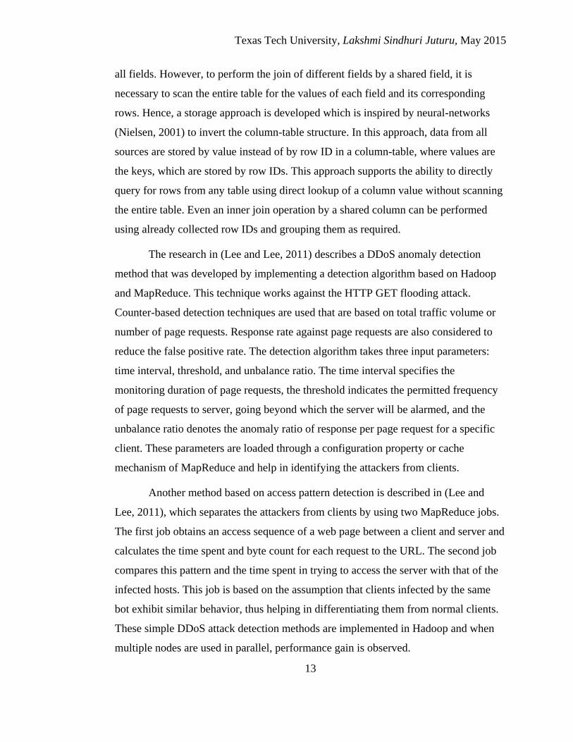
file contains seven columns of data, namely:
1) S.no, which is a sequence number
2) Time, which denotes the seconds’ value at which the request or response occurred
3) Source, which is the IP address of the source
4) Destination, which is the IP address of the destination
5) Length, length of the frame
6) Protocol, which indicates the protocol of the request or response
7) Info, which provides additional information about the request or response
The ‘Info’ column value contains the flags set for the request or response
depending on the protocol used, either ‘TCP’ or ‘ICMP’, and TTL (Time-To-Live)
value. The flags used for a TCP protocol packet can contain one or more flags among
SYN (SYNCHRONIZATION), ACK (ACKNOWLEDGEMENT), FIN (FINISH),
PSH (PUSH) and RST (RESET). Figure 3.1 shows a snapshot of the DDoS attack
dataset retrieved from CAIDA in the form of the .pcap file accessed through
Wireshark.
Figure 3.1: Snapshot of the DDoS attack dataset accessed through Wireshark
In a TCP protocol packet, SYN is used to initiate a connection (Frederick,
2010), ACK is used to acknowledge the validity of the request, FIN is used to
gracefully end the connection, RST is used to abruptly end the connection, and PSH is
used to inform the receiver to distribute the message or data. There are certain key

Texas Tech University, Lakshmi Sindhuri Juturu, May 2015
23
scenarios that are tested to help in identifying abnormal packets when working on the
network traffic datasets, such as 1) packets that do not contain an ACK flag except for
the initial SYN packet, 2) packets that contain SYN and FIN flags together, with or
without other flags in the same packet, 3) packets that contain the FIN flag alone
without any other flags, 4) a packet with no flag at all, and 5) packets that contain the
source or destination port set to zero. All of these scenarios are considered to be
abnormal and help in identifying attack related traffic at the initial stages. Unlike TCP
packets, ICMP packets are not complicated and hence, do not have many
characteristics that can be considered as abnormal. Error messages between two hosts
or a host and a network are transmitted through ICMP packets. In a normal scenario,
no responses are generated for these error messages in order to avoid error message
loops (Frederick, 2010). However, any redirect messages that are sent to a device and
attempt to convince the device that it is an optimal router and route everything to it
can be considered as abnormal. As a result, such ICMP packets are considered fake.
Also, ICMP packets are generally composed of a small header and small payload.
Hence, any ICMP packet that contains a significantly large header or payload should
be considered as abnormal. This is due to the fact that attackers causing DDoS and
other attacks might use ICMP packets as 'containers' that can hide the attack-related
traffic and this could be the reason behind their header or payload being large in size.
Since, all the network data files used in this research are available in ‘.pcap’
format, Wireshark was used to export the data files into .csv (comma separated values)
format. The .csv file contains all the columns separated by commas. However, the
‘info’ column internally contains request or response information along with various
fields separated by commas. Hence, these extra comma characters are removed by
replacing them with a ‘space’ character. Also, all the fields exported from the .pcap
file into .csv format are enclosed with quotation marks. These quotation marks are also
removed as part of the data cleaning process. In the ‘to-victim’ data files, all the
requests are sent to the victim address. Hence, the ‘destination’ column has the same
value throughout the file, which is the host that was attacked. Similarly, the ‘source’

Texas Tech University, Lakshmi Sindhuri Juturu, May 2015
24
column contains the same value in the ‘from-victim’ file. Table 3.1 shows the sample
structure of the ‘from-victim’ dataset converted in .csv format.
Table 3.1: Sample table structure of ‘from-victim’ dataset converted in .csv format
No Time Source Destination Protocol Length Info
349 22.174088 71.126.222.64 198.241.152.229 TCP 40
46426 > http [ACK] Seq=446 Ack=1461 Win=35040 Len=0
350 22.17437 71.126.222.64 198.241.152.229 TCP 40
46426 > http [ACK] Seq=446 Ack=2921 Win=46720 Len=0
351 22.179922 71.126.222.64 198.241.152.229 TCP 40
46426 > http [ACK] Seq=446 Ack=4381 Win=58400 Len=0
352 22.180239 71.126.222.64 198.241.152.229 TCP 40
46426 > http [ACK] Seq=446 Ack=5841 Win=70080 Len=0
353 22.180439 71.126.222.64 198.241.152.229 TCP 40
46426 > http [ACK] Seq=446 Ack=7301 Win=81760 Len=0
In this research, all the rows in the ‘from-victim’ file are taken as they are. But,
the rows of ‘to-victim’ file are appended to the ‘from-victim’ file in such a way that
the ‘source’ column values of ‘to-victim’ are appended to the ‘destination’ column of
‘from-victim’ file. Similarly, ‘destination’ column values of ‘to-victim’ file are
appended to the ‘source’ column of ‘from-victim’ file. A new column ‘Flag’ is
introduced to identify whether the row belongs to the ‘from-victim’ file (Flag: Yes) or
the ‘to-victim’ file (Flag: No) and the existing column ‘S.no’ is removed. By doing the
cross-mapping, the entire dataset can be observed in a unidirectional flow instead of
bi-directional and the computation of all the required factors, such as request, response
and TTL values, become easier since there is no need to distinguish between ‘Source’
and ‘Destination’ fields from each file.
Texas Tech University, Lakshmi Sindhuri Juturu, May 2015
25
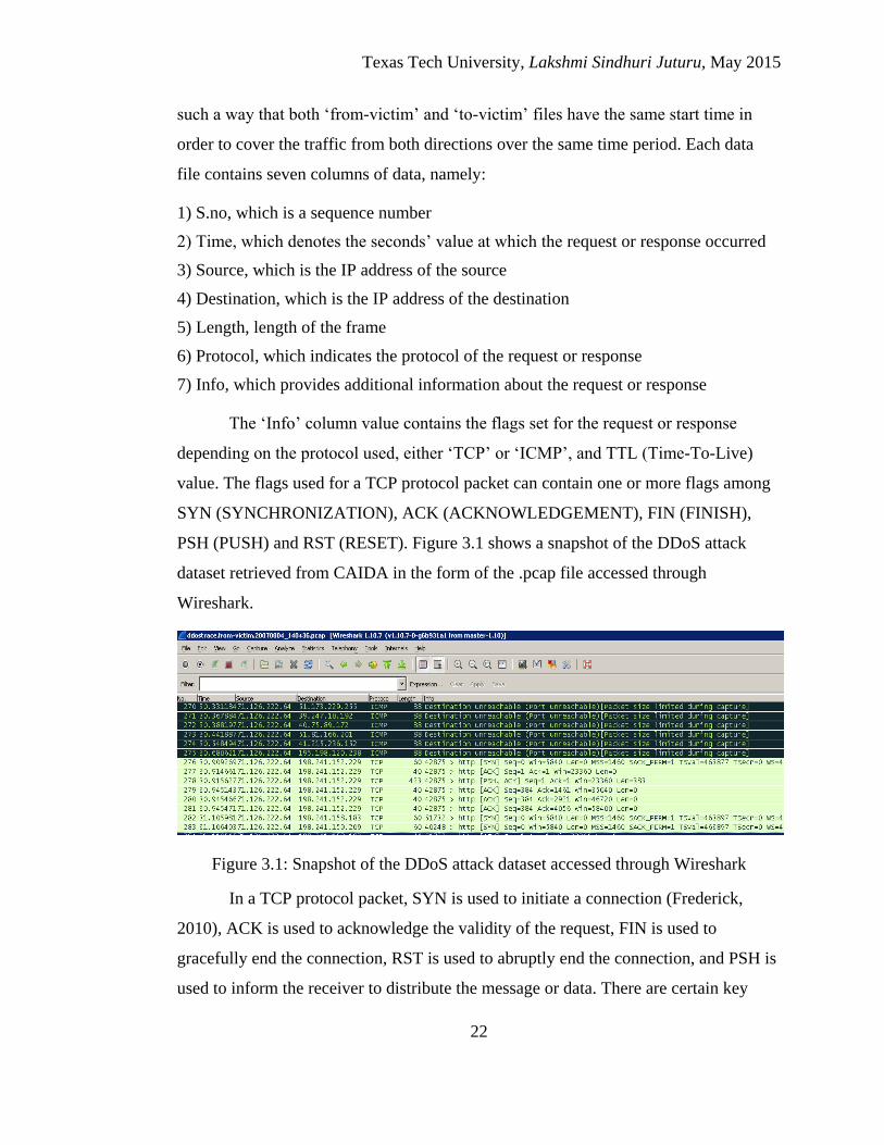
Figure 3.2: Cross-mapping of Source and Destination columns of from-victim and to-
victim files
Figure 3.2 illustrates the cross-mapping of the ‘Source’ and ‘Destination’
columns of ‘to-victim’ data files with that of the ‘from-victim’ data files. Both ‘from-
victim’ and ‘to-victim’ data files contain the columns, 1) S.No (N in Figure 3.2), 2)
Time (T), 3) Source (S), 4) Destination (D), 5) Length (L), 6) Protocol (P), and 7) Info
(I) in a .csv format. The entire ‘Source’ column in every ‘from-victim’ file consists of
same IP address that is the victim’s IP address (in Figure 3.2, v in the ‘from-victim’
file). Similarly, the ‘Destination’ column of every ‘to-victim’ data file consists of the
victim’s IP address (in Figure 3.2, v in the ‘to-victim’ file). Both columns are stored in
the ‘Source’ column of rows table. Similarly, various ‘Destination’ column values of
‘from-victim’ files and ‘Source’ column values of ‘to-victim’ files are stored in the
‘Destination’ column of ‘rows’ table. As shown in Figure 3.2, the ‘Flag’ column
contains ‘Yes’ (y) for all the rows containing data from ‘from-victim’ file and ‘No’ (n)
for the rows containing data from ‘to-victim’ file. When inserting the datasets into the
HBase table structure, the column names are passed as the run time arguments to a
MapReduce program along with the input and output file paths residing on HDFS.
While ‘from-victim’ column names are passed as they are, ‘to-victim’ files are passed

Texas Tech University, Lakshmi Sindhuri Juturu, May 2015
26
as T, D, S, L, P, I, and F as ‘No’ in order to achieve this cross-mapping. The data
stored in the ‘rows’ table is internally loaded into the respective ‘field’ tables, where
each table contains both directions of traffic. Further details about this storage model
are provided in the next chapter.
The DDoS attack datasets obtained from CAIDA are completely anonymized
and the non-attack traffic has been removed as much as possible (The CAIDA, 2007).
Hence, to check the strength of the models developed in this research, real network
traffic from a TTU desktop machine connected to the TTU network has been captured
for five minutes and merged with the attack data. Although this captured data can be
considered as normal, non-attack-related traffic, to attain accuracy in the results, the
sources and destinations obtained in this captured data are verified from the DNS
lookup and are validated against the existing black listings to ensure the authenticity of
the hosts.

Texas Tech University, Lakshmi Sindhuri Juturu, May 2015
27
CHAPTER IV
HBASE DESIGN ALTERNATIVES FOR STORING DATASETS
This chapter describes the design approach chosen for storing the integrated
datasets obtained from the previous chapter. In particular, this chapter 1) lists multiple
use case requirements that are identified for performing data analytics by running data
mining and machine learning techniques on the integrated datasets, 2) describes
various schema designs that were explored for obtaining efficiency in loading the
datasets, as well as retrieving them as per the use case requirements, and 3) illustrates
the evaluations performed on different schema designs and their performance
assessment by comparing the results.
Use Case Requirements
This research has identified certain key use cases that need to be performed on
the network datasets in order to identify the attack-related traffic from the network
traffic. They are:
1) Number of requests made by each unique IP address to the victim
2) Number of responses the same IP address has received from the victim
3) TTL value of each unique IP address that is sending requests to the victim
The TTL values are available in the ‘info’ column for each network packet. These
values are used in calculating the hop-count for each network packet corresponding to
the unique IP address. Hop-count denotes the number of hops a network packet makes
from source to its destination (Gu, 2007). This value is obtained by subtracting the
TTL value available in the ‘info’ column from the standard TTL values. Standard TTL
values are 255, 128, 64, 60, 49, 32, and 30 which depend on the protocol used and the
OS of the machine that generated the packet. Further details on the standard TTL
values and hop-count calculation are provided in the next chapter.
The following use case requirements are related to the ‘Info’ column of ‘to-victim’
data files that are generated while sending requests to the victim (Frederick, 2010).
4) Any network packet that has no flag (such as ACK, SYN, FIN etc.) set

Texas Tech University, Lakshmi Sindhuri Juturu, May 2015
28
5) Any network packet that contain the suspicious combination of SYN and FIN
flags set along with other flags
6) Any network packet that does not contain ACK flag at all except for the initial
connection setup
7) Packets that contain a FIN flag alone without any other flag
These use cases help in generating the statistical data for each unique IP
address that communicated with the victim. The statistical data that is generated for
each IP address based on the given factors help determine whether the IP address is
related to an attacker or not using the data mining algorithms employed in this
research. However, these algorithms cannot be executed directly on a database table
such as HBase or Hive, since each technique expects input in its own type and format.
In this research, Logistic Regression (LR) and Fuzzy k-Means (FKM) algorithms are
used to identify the attack-related traffic. The LR algorithm expects all the factors and
parameters of IP addresses in a .csv format, whereas the FKM algorithm takes input
points represented in an n-dimensional vector space and creates clusters by identifying
the distance among the points. Hence, this research came up with an HBase storage
model where the required data can be efficiently retrieved and used for executing data
mining algorithms.
Design Alternatives
The storage model developed in this research is based on the initial work done
by Stearns (Stearns, 2014), which is a value-based data integration approach that
integrates data by columns instead of rows. Different tables are pooled into a common
collection of columns that can be effectively treated as one single table possessing all
fields. This work is inspired by neural-networks (Nielsen, 2001), which involves
inversion of the column-table structure. In this approach, data from all sources are
stored in a ‘rows’ table, which is in turn divided into many ‘fields’ tables. Here, a
‘rows’ table stores the entire integrated dataset, which further stores the data from
each column in the corresponding ‘fields’ table, which has rowkeys as values followed
by a hash value of ‘Table Id’ and a hash value of ‘Row Id’. This way of storing the
Texas Tech University, Lakshmi Sindhuri Juturu, May 2015
29
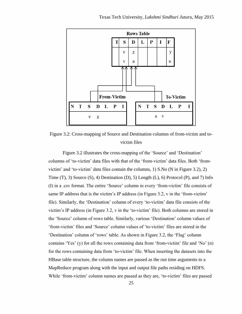
data in HBase is referred as HVID - Hadoop Value-Oriented Integration of Data.
Similarly, a ‘rows’ table also has rowkeys as a hash value of ‘Table Id’ followed by a
hash value of ‘Row Id’. In the HVID model, tables can be directly queried for rows by
direct lookup of a column value without scanning the entire table. Furthermore, an
inner join operation using a shared column among two different tables can be
performed using already collected rowIds and grouping them as required. Also, data
can be quickly merged without having to worry about what columns are used for
merging.
Figure 4.1: Method of storing datasets in rows table followed by field tables
Figure 4.1 shows datasets I and II being inserted into the rows table with the
hash value of ‘Table ID’ followed by a hash value of ‘RowId’ as the rowkey (T1:row1
in the Figure 4.1). A, B, C, D in Figure 4.1 are the column names in the rows table
which stores their corresponding values obtained from the datasets. These values are
inserted into the field tables as well, where each column name in the rows table
becomes the table name of the corresponding field table. Field tables have only one
column that stores only rowkeys that have a value followed by ‘Table ID’ and
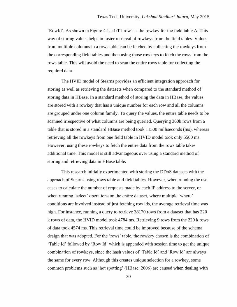
Texas Tech University, Lakshmi Sindhuri Juturu, May 2015
30
‘RowId’. As shown in Figure 4.1, a1:T1:row1 is the rowkey for the field table A. This
way of storing values helps in faster retrieval of rowkeys from the field tables. Values
from multiple columns in a rows table can be fetched by collecting the rowkeys from
the corresponding field tables and then using those rowkeys to fetch the rows from the
rows table. This will avoid the need to scan the entire rows table for collecting the
required data.
The HVID model of Stearns provides an efficient integration approach for
storing as well as retrieving the datasets when compared to the standard method of
storing data in HBase. In a standard method of storing the data in HBase, the values
are stored with a rowkey that has a unique number for each row and all the columns
are grouped under one column family. To query the values, the entire table needs to be
scanned irrespective of what columns are being queried. Querying 360k rows from a
table that is stored in a standard HBase method took 11500 milliseconds (ms), whereas
retrieving all the rowkeys from one field table in HVID model took only 5500 ms.
However, using these rowkeys to fetch the entire data from the rows table takes
additional time. This model is still advantageous over using a standard method of
storing and retrieving data in HBase table.
This research initially experimented with storing the DDoS datasets with the
approach of Stearns using rows table and field tables. However, when running the use
cases to calculate the number of requests made by each IP address to the server, or
when running ‘select’ operations on the entire dataset, where multiple ‘where’
conditions are involved instead of just fetching row ids, the average retrieval time was
high. For instance, running a query to retrieve 38170 rows from a dataset that has 220
k rows of data, the HVID model took 4784 ms. Retrieving 9 rows from the 220 k rows
of data took 4574 ms. This retrieval time could be improved because of the schema
design that was adopted. For the ‘rows’ table, the rowkey chosen is the combination of
‘Table Id’ followed by ‘Row Id’ which is appended with session time to get the unique
combination of rowkeys, since the hash values of ‘Table Id’ and ‘Row Id’ are always
the same for every row. Although this creates unique selection for a rowkey, some
common problems such as ‘hot spotting’ (HBase, 2006) are caused when dealing with

Texas Tech University, Lakshmi Sindhuri Juturu, May 2015
31
large volumes of data. Hot spotting is caused when most of the clients' requests are
directed to a single node or a small set of nodes of a large cluster, keeping other nodes
idle and wasting their resources. Most of the requests that come from the clients are
reads and writes. The problem of hot spotting can lead to consequences such as
unavailability of the hot region, performance degradation, and resource wastage of
cold regions. If all the regions belong to a standalone machine, then other regions are
most likely unavailable. These problems can be eradicated by distributing the data in
such a way that it has a well load-balanced cluster that can be achieved by changing
the row key design. Hence, rowkeys are the single most important aspect of HBase
table design (Khurana, 2012).
Hence, this research has explored various HBase table schema designs by
experimenting with three different rowkey designs and identifying the best possible
design that meets the use case requirements of this research. The three rowkey designs
that were tested are:
1) The ‘S.no’ field as the rowkey with a unique number for each row
2) The ‘Time’ field concatenated with ‘S.no’ as the rowkey
3) The ‘Destination’ field concatenated with ‘S.no’ as the rowkey
Among these three designs, the third one that has ‘Destination’ concatenated with
‘S.no’ gave the best data retrieval times (as shown in Table 4.1). This design has
proven to take less time to store the datasets as well as less time to retrieve that data
compared to the HVID model. Hence, this rowkey design is integrated with the HVID
model and the datasets are cross-mapped (as shown in Figure 3.2) to increase the
efficiency while retrieving the data (as explained in the Chapter 3). This model is
referred to as the HBaseSchema model. The results of the three schema designs that
were tested and the comparisons of the HVID model and the HBaseSchema model in
storing and retrieving the datasets are provided in the “Design Evaluation” section in
this chapter.
After storing the DDoS datasets in the HBaseSchema model, the statistical data
is obtained by running the use cases (as mentioned in the “Use Case Requirements”
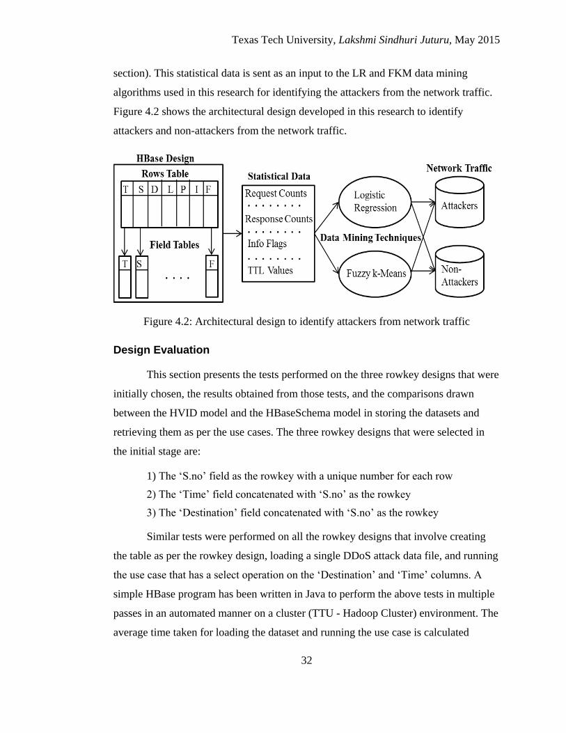
Texas Tech University, Lakshmi Sindhuri Juturu, May 2015
32
section). This statistical data is sent as an input to the LR and FKM data mining
algorithms used in this research for identifying the attackers from the network traffic.
Figure 4.2 shows the architectural design developed in this research to identify
attackers and non-attackers from the network traffic.
Figure 4.2: Architectural design to identify attackers from network traffic
Design Evaluation
This section presents the tests performed on the three rowkey designs that were
initially chosen, the results obtained from those tests, and the comparisons drawn
between the HVID model and the HBaseSchema model in storing the datasets and
retrieving them as per the use cases. The three rowkey designs that were selected in
the initial stage are:
1) The ‘S.no’ field as the rowkey with a unique number for each row
2) The ‘Time’ field concatenated with ‘S.no’ as the rowkey
3) The ‘Destination’ field concatenated with ‘S.no’ as the rowkey
Similar tests were performed on all the rowkey designs that involve creating
the table as per the rowkey design, loading a single DDoS attack data file, and running
the use case that has a select operation on the ‘Destination’ and ‘Time’ columns. A
simple HBase program has been written in Java to perform the above tests in multiple
passes in an automated manner on a cluster (TTU - Hadoop Cluster) environment. The
average time taken for loading the dataset and running the use case is calculated
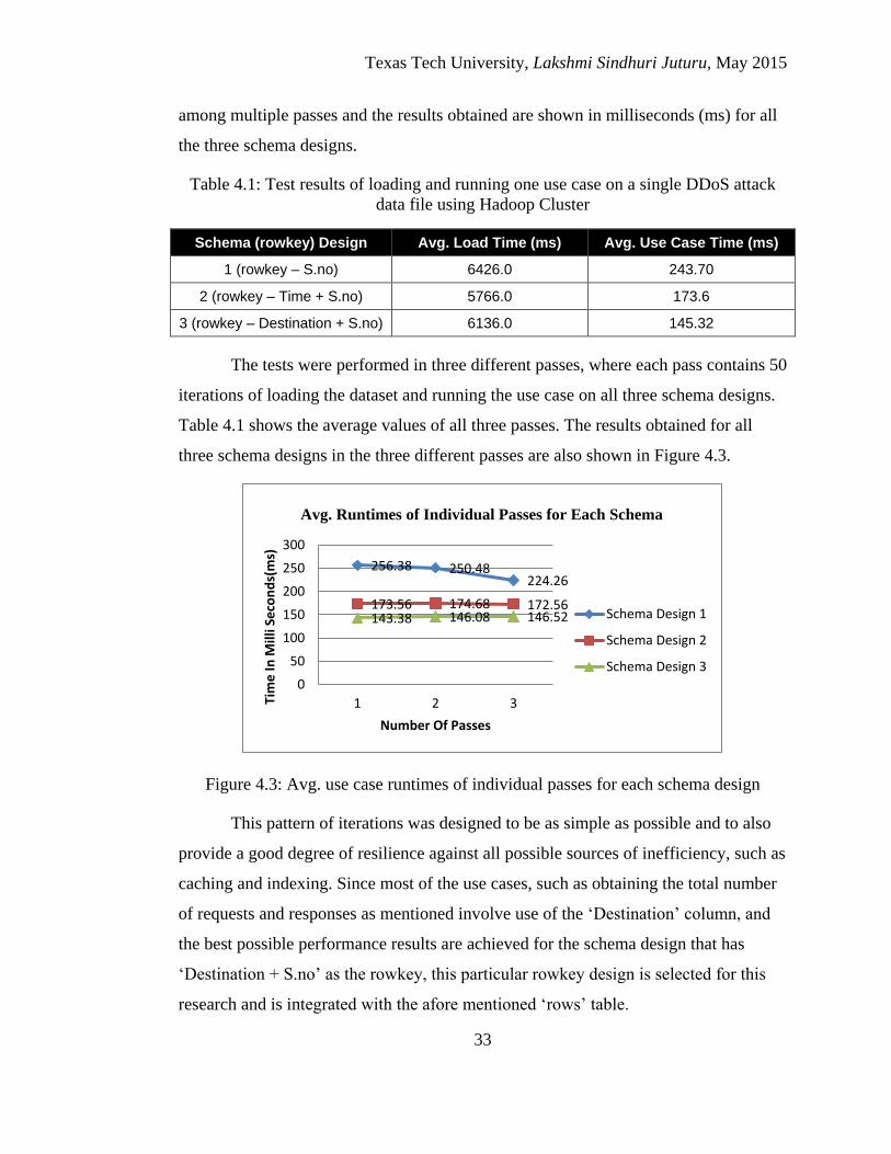
Texas Tech University, Lakshmi Sindhuri Juturu, May 2015
33
among multiple passes and the results obtained are shown in milliseconds (ms) for all
the three schema designs.
Table 4.1: Test results of loading and running one use case on a single DDoS attack
data file using Hadoop Cluster
Schema (rowkey) Design Avg. Load Time (ms) Avg. Use Case Time (ms)
1 (rowkey – S.no) 6426.0 243.70
2 (rowkey – Time + S.no) 5766.0 173.6
3 (rowkey – Destination + S.no) 6136.0 145.32
The tests were performed in three different passes, where each pass contains 50
iterations of loading the dataset and running the use case on all three schema designs.
Table 4.1 shows the average values of all three passes. The results obtained for all
three schema designs in the three different passes are also shown in Figure 4.3.
Figure 4.3: Avg. use case runtimes of individual passes for each schema design
This pattern of iterations was designed to be as simple as possible and to also
provide a good degree of resilience against all possible sources of inefficiency, such as
caching and indexing. Since most of the use cases, such as obtaining the total number
of requests and responses as mentioned involve use of the ‘Destination’ column, and
the best possible performance results are achieved for the schema design that has
‘Destination + S.no’ as the rowkey, this particular rowkey design is selected for this
research and is integrated with the afore mentioned ‘rows’ table.
256.38 250.48 224.26
173.56 174.68 172.56 143.38 146.08 146.52
0
50
100
150
200
250
300
1 2 3Tim
e In
Mill
i Se
con
ds(
ms)
Number Of Passes
Avg. Runtimes of Individual Passes for Each Schema
Schema Design 1
Schema Design 2
Schema Design 3
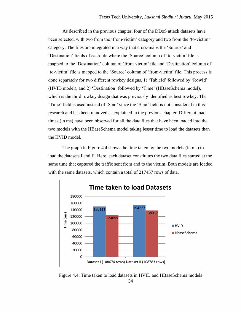
Texas Tech University, Lakshmi Sindhuri Juturu, May 2015
34
As described in the previous chapter, four of the DDoS attack datasets have
been selected, with two from the ‘from-victim’ category and two from the ‘to-victim’
category. The files are integrated in a way that cross-maps the ‘Source’ and
‘Destination’ fields of each file where the ‘Source’ column of ‘to-victim’ file is
mapped to the ‘Destination’ column of ‘from-victim’ file and ‘Destination’ column of
‘to-victim’ file is mapped to the ‘Source’ column of ‘from-victim’ file. This process is
done separately for two different rowkey designs, 1) ‘TableId’ followed by ‘RowId’
(HVID model), and 2) ‘Destination’ followed by ‘Time’ (HBaseSchema model),
which is the third rowkey design that was previously identified as best rowkey. The
‘Time’ field is used instead of ‘S.no’ since the ‘S.no’ field is not considered in this
research and has been removed as explained in the previous chapter. Different load
times (in ms) have been observed for all the data files that have been loaded into the
two models with the HBaseSchema model taking lesser time to load the datasets than
the HVID model.
The graph in Figure 4.4 shows the time taken by the two models (in ms) to
load the datasets I and II. Here, each dataset constitutes the two data files started at the
same time that captured the traffic sent from and to the victim. Both models are loaded
with the same datasets, which contain a total of 217457 rows of data.
Figure 4.4: Time taken to load datasets in HVID and HBaseSchema models
150111 154227
124655 138017
0
20000
40000
60000
80000
100000
120000
140000
160000
180000
Dataset I (108674 rows) Dataset II (108783 rows)
Tim
e (
ms)
Time taken to load Datasets
HVID
HbaseSchema
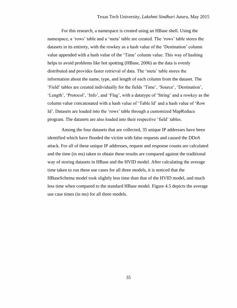
Texas Tech University, Lakshmi Sindhuri Juturu, May 2015
35
For this research, a namespace is created using an HBase shell. Using the
namespace, a ‘rows’ table and a ‘meta’ table are created. The ‘rows’ table stores the
datasets in its entirety, with the rowkey as a hash value of the ‘Destination’ column
value appended with a hash value of the ‘Time’ column value. This way of hashing
helps to avoid problems like hot spotting (HBase, 2006) as the data is evenly
distributed and provides faster retrieval of data. The ‘meta’ table stores the
information about the name, type, and length of each column from the dataset. The
‘Field’ tables are created individually for the fields ‘Time’, ‘Source’, ‘Destination’,
‘Length’, ‘Protocol’, ‘Info’, and ‘Flag’, with a datatype of ‘String’ and a rowkey as the
column value concatenated with a hash value of ‘Table Id’ and a hash value of ‘Row
Id’. Datasets are loaded into the ‘rows’ table through a customized MapReduce
program. The datasets are also loaded into their respective ‘field’ tables.
Among the four datasets that are collected, 35 unique IP addresses have been
identified which have flooded the victim with false requests and caused the DDoS
attack. For all of these unique IP addresses, request and response counts are calculated
and the time (in ms) taken to obtain these results are compared against the traditional
way of storing datasets in HBase and the HVID model. After calculating the average
time taken to run these use cases for all three models, it is noticed that the
HBaseSchema model took slightly less time than that of the HVID model, and much
less time when compared to the standard HBase model. Figure 4.5 depicts the average
use case times (in ms) for all three models.
Texas Tech University, Lakshmi Sindhuri Juturu, May 2015
36
Figure 4.5: Avg. time taken to run use cases in Standard HBase, HVID and
HBaseSchema models
Using this model, required factors such as the total number of requests and the
total number of responses in the datasets to be fetched and calculated per second in
order to obtain the request/response ratio per second. TTL values are also fetched for
all the unique IP addresses that were identified previously, in order to identify the
network packets that have abnormal TTL values. Data mining and machine learning
techniques are then used on these factors to identify the attack-related traffic from the
network traffic. The details of these results are provided in the next chapter.
All of these tests have been performed on IBM BigInsights v2.1.2 that comes
with an installation of Hadoop, HBase and other big data tools, running on a 64-bit
virtual Linux machine. This was installed on a standalone Windows-7 64 bit machine
that has 8 GB RAM and a 2.99 GHz processor.
5250.1
4005.7 3863.1
3600
3800
4000
4200
4400
4600
4800
5000
5200
5400
Standard Hbase HVID HbaseSchema
Tim
e (
ms)
Avg. Usecase Time (ms)
Avg. Usecase Time (ms)

Texas Tech University, Lakshmi Sindhuri Juturu, May 2015
37
CHAPTER V
DATA MINING AND MACHINE LEARNING APPLIED TO
CYBERSECURITY DATASETS
This research aims to create a model using Hadoop and HBase for storing the
integrated datasets and efficiently retrieve statistical data associated with the datasets,
which can be used to run data mining and machine learning algorithms to identify
attack-related traffic from regular traffic. In the previous Chapters 3 and 4, various
HBase models and schema designs have been discussed that provide efficient ways for
data storage and retrieval. This chapter provides details about the data mining and
machine learning techniques such as the Logistic Regression (LR) classification
algorithm (Komarek, 2004) and the Fuzzy k-Means (FKM) clustering algorithm
(Bezdek, 1981), applied on the statistical data to identify the attack related traffic. This
research has experimented with the two algorithms to attain accuracy in the results and
to identify the best algorithm that is potentially capable of identifying attackers in the
network datasets. Comparisons drawn between the results obtained from the LR and
FKM algorithms are also described in this chapter.
Use of Logistic Regression
The LR algorithm is a Supervised Learning algorithm (LR) whereas the FKM
algorithm is an Unsupervised Learning algorithm. Machine Learning is a concept of
Artificial Intelligence using which, a machine can learn from the data without having
the need to explicitly write a program (Kovahi, 1988). Machine learning algorithms
operate by generating a model from the sample data provided to them. This type of
algorithm where sample input and output are provided, and rules are generated to map
the input to the output is called Supervised Learning (Russell, 2003). Examples of
Supervised Learning algorithms are Logistic Regression, Decision Trees, Support
Vector Machine (SVM) and k-Nearest Neighbor (KNN). On the other hand, machine
learning algorithms that do not take any labeled data but identify a hidden structure
and model in the data are termed as Unsupervised Learning algorithms. Examples of
Unsupervised Learning algorithms are k-Means, Fuzzy k-Means algorithms and
hidden Markov models.
Texas Tech University, Lakshmi Sindhuri Juturu, May 2015
38
This research preferred the use of LR for its ability to provide quick and
accurate results while performing classification, as well as its simplicity over other
supervised learning algorithms such as Decision Trees (Mohri, 2012). The LR
algorithm has been employed in the past in cases of fraud detection or spam detection
(Owen, 2012). It is best preferred in scenarios that produce output in a binary form of
0 or 1. For instance, classifying an email as a spam or non-spam is denoted as 1 or 0.
This research has also used Apache Mahout (Mahout, 2009), which is an open
source platform that provides implementations for various classification, clustering,
association, and recommendation-related algorithms. Since, Mahout runs on top of
Hadoop, the algorithms can be run on a single machine or as a MapReduce program
that takes input files from an HDFS cluster. Although there is no single algorithm that
works the best for all problems, the user must identify which algorithm best suits a
given use case. This research utilizes the LR classification algorithm provided by
Mahout that helps in easy and automatic processing of large datasets to classify each
IP address either as an attacker or a non-attacker.
LR provided by Mahout uses a simple, sequential (non-parallel) method called
Stochastic Gradient Descent (SGD) that has a low overhead when compared to other
methods when working on datasets (Owen et al., 2012). Although SGD is non-
parallel, it's invariably fast and can handle large training sets that contain millions of
samples. SGD provided by Mahout is an online learning algorithm, which means that
models can be learned in an incremental fashion and the performance of each model
can be tested while the system continues to run. In this algorithm, every training
sample is used to tweak the model until the best possible model is attained. This
process is repeated over all the available training examples. Mahout has built-in
classes such as CrossFoldLearner that can perform the online evaluation, including
cross-validation. Cross-validation refers to dividing the dataset into 5 equal sets (20%
each) out of which, one set (20%) is used for evaluation and the remaining 80% data is
used for training. This is repeated in a round-robin fashion such that for all the
possible five runs, five different sets are used for evaluation, while the rest is used for
training the model. At the end of the five runs, the best model that fits the dataset can
Texas Tech University, Lakshmi Sindhuri Juturu, May 2015
39
be identified. This method also avoids the problem of overfitting. Overfitting refers to
the scenario, where the model works fine on the training data that is used for
generating the model, but fails to classify new samples when a new set of data is
introduced for evaluation (Pedregosa, 2011).
Since the datasets obtained from CAIDA contain purely attack traffic, with all
non-attack traffic removed, network traffic has been captured for five minutes from a
TTU desktop machine connected to the TTU network and merged with the attack data
as described in the previous section. Also, it might be evident that the data files
obtained from CAIDA contain purely attack data and the data files generated from
TTU machine contain purely non-attack data. However, it helps to generate a robust
model using the LR algorithm by passing this mixture of data files as training samples
for the learning phase of the algorithm. Moreover, this model can be tested by running
it on any network traffic dataset just by using the required statistical data for all the
suspicious IP addresses as the input file.
The datasets that were previously integrated and stored in the HBase model, as
described in the previous section, contain over 200k rows of data. Among these
various rows of data that have both requests and responses, only 34 unique IP
addresses are found. For all 34 unique IP addresses, the number of requests and
responses generated per second are calculated and an input file in the form of .csv is
created. The same process is repeated for the non-attack traffic captured from the TTU
machine, by identifying 7 unique IP addresses and calculating their request and
response counts per second. The statistical data obtained from the non-attack data file
is merged with that of the attack data file.
Logistic Regression algorithm is executed through Mahout in two stages,
namely TrainLogistic and RunLogistic. During the TrainLogistic phase, a training
dataset that constitutes about 80% of the original input dataset is passed and this
algorithm takes several key arguments as inputs. The arguments are:
1) input - path for the input file (.csv format preferred)
2) output - path and name of the model, where the generated model is placed

Texas Tech University, Lakshmi Sindhuri Juturu, May 2015
40
3) predictors - list of predictor variables, which help in classifying the target
4) types - data types of each predictor variable that can be a numeric, word, or text
5) categories - number of categories the target variable contains
6) passes - number of times the input file should be re-examined
(small input files require a dozen times)
7) target - a field in the input file that contains the target variable
8) rate - sets the initial learning rate (usually higher value required for large input
files), and
9) features - sets the size of the internal feature vector that is used in building the
model
Once the model is generated, it outputs the coefficients (B0, B1, B2 ... Bn)
calculated for all the predictor variables (x1, x2 … xn) as well as intercept term (which
is a built-in predictor variable for LR). This model is used to perform the evaluation of
classifying the samples from the given input dataset by running the RunLogistic
algorithm through Mahout. This algorithm takes fewer number of arguments
compared to that of the training phase. The arguments are:
1) input - path for the input file that needs to be evaluated
2) model - path for the model that is used to evaluate the input data
3) auc - (area under curve) that determines the strength and quality of the model,
which ranges from 0 to 1, with 1 considered as the best
4) scores - prints the target variable value along with their scores for each input value
5) confusion - prints the confusion matrix that determines the number of correctly and
incorrectly classified samples.
All the coefficient values obtained from the model and predictor values fetched
from the input data file are substituted in the formula below and the function values
are computed. The output values that are close to 1 are labeled as 1 and the values that
are close to 0 are labeled as 0 under the target column.
Logistic Regression Formula: 1/ [1+e–(B0+B1X1+B2X2+ … +BnXn)
]
Initially, two factors are considered as predictor variables for generating the
model, 1) requests per second calculated for each unique IP address, and 2)
request/response ratio per second. However, the auc that determines the strength and

Texas Tech University, Lakshmi Sindhuri Juturu, May 2015
41
quality of the model was 0.61, which is considered as above average. For a model, the
auc values range from 0 to 1, where 1 indicates that the model is best, 0 indicates that
it is a perverse model, and 0.5 is considered as average or random. Out of 23 samples,
20 were classified by the model when run on the same input dataset that is used to
generate the model. Upon running the model on newly added samples in addition to
the existing ones, the auc value was dropped to 0.5 which is considered as an average
value.
Table 5.1: Sample values (poor results) of the model generated using a single dataset
Target Model-Output Log-Likelihood
0 0.000 -0.000000
0 0.000 -0.000000
1 1.000 -0.000000
1 0.000 -100.000000
AUC = 0.61
Confusion: [[19.0, 3.0], [0.0, 1.0]] //Confusion Matrix
Table 5.1 shows four rows out of the 23 rows obtained by running the model
on the same sample dataset that was used to generate this model. The Target variable
shows whether each IP address is classified as an attacker (0) or non-attacker (1).
Model-Output presents the frequency of each value listed in the input set, and Log-
Likelihood describes the logarithmic values of the probability of each event (here, IP
address) that is likely to happen again. Another important performance metric in the
LR algorithm is the Confusion Matrix, which determines the number of correctly
classified and incorrectly classified samples. Using this sample model that was
generated, 20 (19+1 in the matrix) samples are correctly classified, with 19 as
attackers (0) and 1 non-attacker (1) and 3 (3+0) samples are incorrectly classified,
which are false-positives that indicates 3 samples that are non-attackers are incorrectly
classified as attackers. Although, the model is able to classify 20 samples out of 23
correctly, it has poor auc, model-output, and log values, and is therefore considered as
an unfit model.
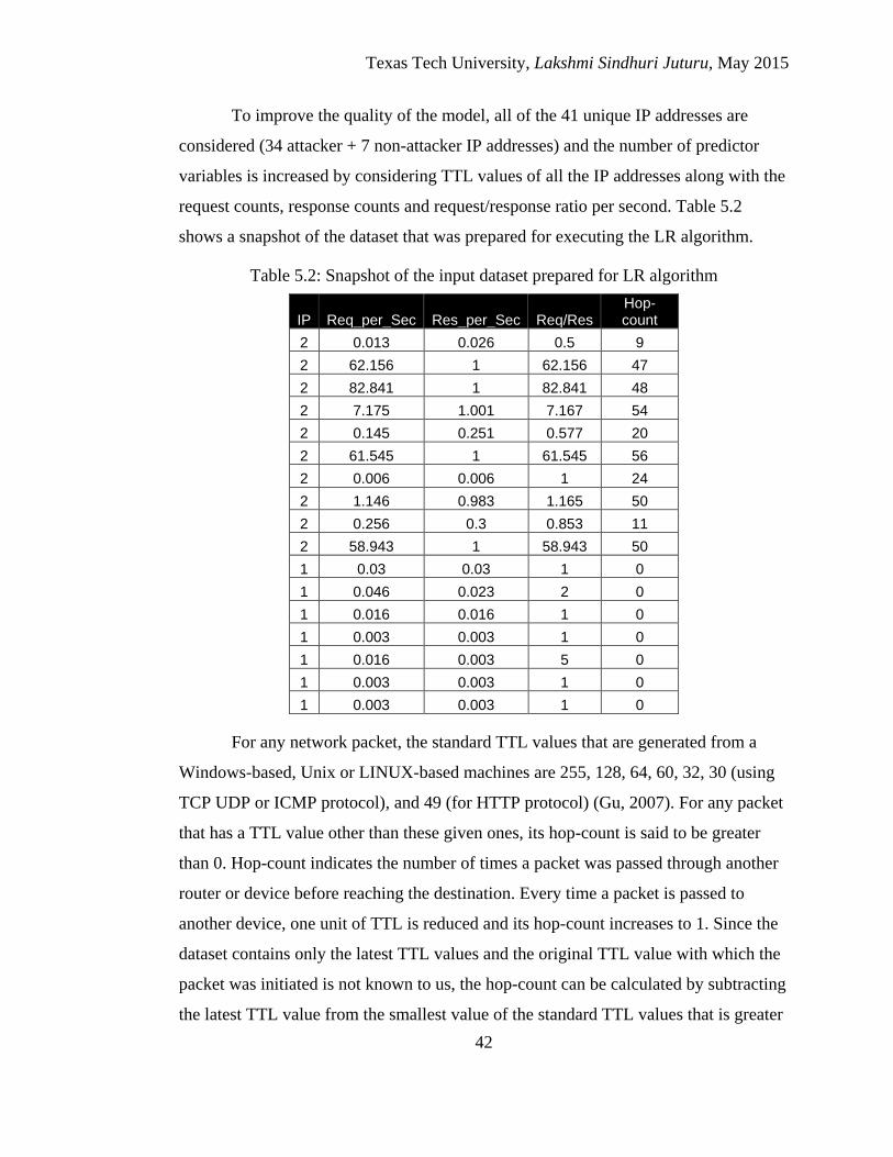
Texas Tech University, Lakshmi Sindhuri Juturu, May 2015
42
To improve the quality of the model, all of the 41 unique IP addresses are
considered (34 attacker + 7 non-attacker IP addresses) and the number of predictor
variables is increased by considering TTL values of all the IP addresses along with the
request counts, response counts and request/response ratio per second. Table 5.2
shows a snapshot of the dataset that was prepared for executing the LR algorithm.
Table 5.2: Snapshot of the input dataset prepared for LR algorithm
IP Req_per_Sec Res_per_Sec Req/Res Hop-count
2 0.013 0.026 0.5 9
2 62.156 1 62.156 47
2 82.841 1 82.841 48
2 7.175 1.001 7.167 54
2 0.145 0.251 0.577 20
2 61.545 1 61.545 56
2 0.006 0.006 1 24
2 1.146 0.983 1.165 50
2 0.256 0.3 0.853 11
2 58.943 1 58.943 50
1 0.03 0.03 1 0
1 0.046 0.023 2 0
1 0.016 0.016 1 0
1 0.003 0.003 1 0
1 0.016 0.003 5 0
1 0.003 0.003 1 0
1 0.003 0.003 1 0
For any network packet, the standard TTL values that are generated from a
Windows-based, Unix or LINUX-based machines are 255, 128, 64, 60, 32, 30 (using
TCP UDP or ICMP protocol), and 49 (for HTTP protocol) (Gu, 2007). For any packet
that has a TTL value other than these given ones, its hop-count is said to be greater
than 0. Hop-count indicates the number of times a packet was passed through another
router or device before reaching the destination. Every time a packet is passed to
another device, one unit of TTL is reduced and its hop-count increases to 1. Since the
dataset contains only the latest TTL values and the original TTL value with which the
packet was initiated is not known to us, the hop-count can be calculated by subtracting
the latest TTL value from the smallest value of the standard TTL values that is greater
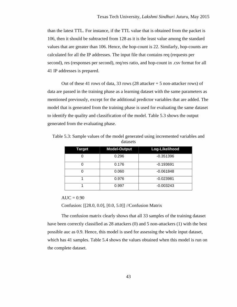
Texas Tech University, Lakshmi Sindhuri Juturu, May 2015
43
than the latest TTL. For instance, if the TTL value that is obtained from the packet is
106, then it should be subtracted from 128 as it is the least value among the standard
values that are greater than 106. Hence, the hop-count is 22. Similarly, hop-counts are
calculated for all the IP addresses. The input file that contains req (requests per
second), res (responses per second), req/res ratio, and hop-count in .csv format for all
41 IP addresses is prepared.
Out of these 41 rows of data, 33 rows (28 attacker + 5 non-attacker rows) of
data are passed in the training phase as a learning dataset with the same parameters as
mentioned previously, except for the additional predictor variables that are added. The
model that is generated from the training phase is used for evaluating the same dataset
to identify the quality and classification of the model. Table 5.3 shows the output
generated from the evaluating phase.
Table 5.3: Sample values of the model generated using incremented variables and
datasets
Target Model-Output Log-Likelihood
0 0.296 -0.351396
0 0.176 -0.193691
0 0.060 -0.061848
1 0.976 -0.023981
1 0.997 -0.003243
AUC = 0.90
Confusion: [[28.0, 0.0], [0.0, 5.0]] //Confusion Matrix
The confusion matrix clearly shows that all 33 samples of the training dataset
have been correctly classified as 28 attackers (0) and 5 non-attackers (1) with the best
possible auc as 0.9. Hence, this model is used for assessing the whole input dataset,
which has 41 samples. Table 5.4 shows the values obtained when this model is run on
the complete dataset.

Texas Tech University, Lakshmi Sindhuri Juturu, May 2015
44
Table 5.4: Sample values of the model evaluated on the complete input dataset
Target Model-Output Log-Likelihood
0 0.177 -0.194467
0 0.209 -0.234551
0 0.060 -0.061848
1 0.976 -0.023981
1 0.998 -0.002318
AUC = 0.89
Confusion: [[34.0, 0.0], [0.0, 7.0]] //Confusion Matrix
Similarly, when the same model is run on the full input dataset that has new
samples other than the one used for training, the auc value was 0.89 and all samples
were correctly identified as 34 attackers and 7 non-attackers.
Use of Fuzzy k-Means
As a data mining technique, this research has used the Fuzzy k-Means (FKM)
(Bezdek, 1981) clustering algorithm for grouping certain IP addresses that exhibit a
similar type of characteristics under one cluster, which helps in segregating attack-
related traffic from regular network traffic. Fuzzy k-Means was chosen for its ability
to identify soft clusters, unlike the original k-Means algorithm (MacQueen, 1967),
which identifies only hard clusters. In a soft cluster, any given point can be placed in
more than a single cluster, which creates overlapping clusters in the dataset. In a hard
cluster, each point belongs to exactly one cluster, thus ruling out the possibility of
identifying attack-related characteristics in normal traffic. However, the FKM
algorithm checks the possibility of each point with an affinity value towards belonging
to other clusters. This affinity value of each point is directly proportional to the
distance of the point from the centroid of each cluster. Hence, the FKM algorithm
creates soft clusters as an extension to the k-Means algorithm (Owen, 2012). FKM
works best in cases where the clusters might be overlapped or mixed with each other
and the distance among the points is not linear, where a k-Means cannot provide a
better solution.

Texas Tech University, Lakshmi Sindhuri Juturu, May 2015
45
The FKM algorithm has built-in methods for measuring the distance and
representing each point in an n-dimensional vector space. Similar to that of an LR
algorithm input file, the same characteristics are considered in the input file of the
FKM algorithm: the number of requests per second, the number of responses per
second, and the hop-count value for all 41 unique IP addresses. However, unlike the
LR algorithm, FKM doesn’t take predictor variables and solely depends on the input
points represented in vector space and the distance of each point with its adjacent
points. Hence, in order to represent all the key characteristics of each network packet
through a single point that can be used in forming clusters, the characteristics observed
for each IP address, request per second, response per second and the hop-count are
added to form a single value for each IP address. This is done in order to give equal
weightage to all the parameters as they all have an equal role in determining an IP
address as an attacker or non-attacker. This algorithm is executed in four steps when
working on a single machine or using MapReduce on a cluster environment.
Step 1:
In the first analysis step, the input file is converted into a sequence file. Since
Mahout runs on top of Hadoop, Mahout provides a number of Hadoop classes that
convert all input files automatically into a sequence file. This sequence file is in turn
converted into a vector file, which is taken as the argument for running the FKM
algorithm. This process is explained in the step 2. The SequenceFile class provided by
Mahout converts each and every value to the form of a (key, value) pair, where the
key is the document name and the value is each number obtained from the input file.
The arguments passed to this class are:
1) input - path that specifies the directory that contains all the input files
2) output - path that specifies the directory where the sequence file is created
3) method - method that is used to execute this step, which can be sequential or
mapreduce
All the remaining parameters are optional and this step can be executed with
the default values provided by the Java class.
Texas Tech University, Lakshmi Sindhuri Juturu, May 2015
46
Step 2:
The next step of the analysis process is to generate vectors from the sequence
file created in the previous step. The Seq2sparse class takes the sequence file as an
input and creates tokenized documents in the form of <docID, tokenizedDoc> pairs
and vectorized documents in the form of <docID, TF-IDF vector>. TF-IDF refers to
Term Frequency and Inverse Document Frequency, which is used to identify the
importance and frequency of each value in the input file or word in case of text-related
documents. TF gives the number of times each word has occurred in the document and
IDF refers to the frequency of the same value in the other documents in order to
identify whether it's a common or rare occurrence in the input files. This factor is not
applicable for the given input file, since it is a single file. In addition to the tokenized
documents, The seq2sparse class also creates sequence files for:
1) dictionary - index for each value followed by the value <valueIndex,
value>
2) word frequency count - index for each value followed by its count
<valueIndex, count>, and
3) document frequency count - index for each value followed by DF count
<valueIndex, DFCount>.
The DFCount is not applicable for the given input file since it is a single file.
This step takes several input parameters other than the usual input and output
arguments. For the 'weight' argument, the value can be specified as TF instead of TF-
IDF, as IDF is not applicable for a single input file. The named vector argument can
be set to true, so that the output vectors that are created will be named.
Step 3:
The third analysis step is to run the FKM algorithm using the TF-IDF vectors
created in the previous step, along with a few key arguments, such as:
1) input - path to the directory that contains the vector files created in the
previous steps
2) output - path to the directory where output files are created
Texas Tech University, Lakshmi Sindhuri Juturu, May 2015
47
3) clusters - path to a new directory where the output clusters are created.
4) distance measure - classname of the distance measure that is preferred
(Euclidean or Cosine)
5) x - maximum number of iterations that is preferred.
6) m - fuzzyness argument that specifies the coefficient for normalization. If
specified as 1, then it is treated as k-Means algorithm.
7) k - number of clusters that need to be created.
Upon successful completion of this step, 'k' (given) number of clusters will be
created in the specified folder for clusters, which contains a separate folder for each
cluster, named from cluster-0, cluster-1, up to cluster-N. Each cluster folder contains a
sequence file that has an identifier followed by the value present in that soft cluster.
Also, the output folder specified contains another sequence file that has all the
clustered points in a (key, value) format, where each key is the clusterId.
The final step is performed using the clusterdump tool that converts the
sequence files of each cluster into a readable format, listing the centroids and all the
values present in that cluster. To perform this step, the input path is mentioned as the
final cluster folder and if output path is specified, the clusters are written to that file,
otherwise the output is printed on the shell itself. The dictionary file created in the
second step can be provided optionally as an argument, if required. Also,
'dictionaryType' should be mentioned as 'sequencefile' since the input file used for
FKM is not a text file.
The input file passed to the first step of running the FKM algorithm is the list
of 41 IP values (given below), which are placed linearly without any commas in a text
file:
[15.838, 9.039, 110.156, 131.841, 62.176, 9.293, 9.105, 9.458, 20.396, 118.545,
24.012, 52.129, 11.556, 109.943, 54.616, 17.04, 17.07, 20.053, 20.059, 4.26, 112.616,
64.755, 61.63, 19.252, 22.06, 15.039, 9.009, 20.15, 5.483, 10.48, 15.02, 52.006,
16.006, 11.106, 0.06, 0.069, 0.032, 0.006, 0.019, 0.006, 0.006]

Texas Tech University, Lakshmi Sindhuri Juturu, May 2015
48
Using the FKM algorithm, 3 clusters C1, C2, and C3 are created with three
centroids for each cluster, highlighted in bigger size in Figure 4.6. The points grouped
in cluster C1 are non-attackers and the remaining points grouped in cluster C2 and C3
are all attackers. In the Figure 4.6, clusters C1 and C2 share the two points, 4.26 and
5.483 as they are created as soft clusters and these two points are similar to that of the
points available in both the clusters. Although these two points are grouped with
cluster C1, which contains non-attacker IP values, these points are attackers and
should be placed in cluster C2. This is both an advantage and disadvantage of using
the FKM algorithm. The disadvantage is that they are placed in cluster C1 in spite of
being attackers. However, it is more advantageous to use the FKM algorithm because
these two points are considered in cluster C2 as well giving a need for attention.
Cluster C3 has more clear values and is a hard cluster because it is not sharing values
with any other cluster. Also, if there are any common points shared between clusters
C2 and C3, this sharing would be acceptable since both clusters contain attackers. The
same input data file run in the k-means algorithm gave a clear cluster of C1 and C2
with these two points being placed in cluster C1 instead of cluster C2. In a real
scenario, these 2 points would have gone unnoticed as they are grouped with non-
attackers, which is dangerous as they are false-negatives.
Cluster C1 contains 9 points with 1 as the centroid:
[0.06, 0.069, 0.032, 0.006, 0.019, 0.006, 0.006, 4.26, 5.483]
Cluster C2 contains 23 points with a centroid of 15 and sharing 4.26 and 5.483 points
with cluster 1:
[15.838, 9.039, 9.293, 9.105, 9.458, 20.396, 24.012, 11.556, 17.04, 17.07, 20.053,
20.059, 19.252, 22.06, 15.039, 9.009, 20.15, 10.48, 15.02, 16.006, 11.106, 4.26,
5.483]
Cluster C3 contains the remaining 11 points with a centroid of 84:
[110.156, 131.841, 62.176, 118.545, 52.129, 109.943, 54.616, 112.616, 64.755, 61.63,
52.006]

Texas Tech University, Lakshmi Sindhuri Juturu, May 2015
49
Figure 4.6: The three clusters formed using FKM algorithm
Comparison and Analysis of LR and FKM Algorithms
This research has experimented with two algorithms that are potentially
capable of segregating the attack-related traffic from regular network traffic. Logistic
Regression is a classification algorithm that is an example of a supervised learning
technique, whereas Fuzzy k-Means is a clustering algorithm that provides an example
of an unsupervised learning technique that does not require any labeled data or
training phases. Although these two algorithms are best in their own ways, Logistic
Regression took 250 to 300 ms for the combined effort of the training and execution
phases, whereas the FKM algorithm took around 700 to 900 ms for each stage. Hence,
the combined effort for all four stages is 4000 ms. Although finalizing the training
model in the LR algorithm may take more number of passes and much time needed to
execute, once the model is finalized, the Logistic Regression algorithm classifies
attackers and non-attackers in less time compared to the FKM algorithm.
Besides taking less time for execution, Logistic Regression gives about 90%
accuracy when all the training scenarios are taken into consideration. The finalized
Texas Tech University, Lakshmi Sindhuri Juturu, May 2015
50
model mentioned in the previous section classified all 41 samples as 34 attackers and
7 non-attackers, identifying 100% accurately. The FKM algorithm accurately grouped
39 out of 41 samples, with 2 samples being shared among two attacker and non-
attacker clusters. Since the FKM algorithm creates clusters of closely-related points, a
few attacker IP addresses that have fewer counts similar to that of a non-attacker IP
addresses are grouped together. Due to this, 2 attackers are incorrectly grouped with
non-attackers. Thus, the FKM algorithm exhibited 95% accuracy in creating clusters
of attackers and non-attackers in the given datasets. In this research, only five datasets
(1 non-attacker + 4 attacker datasets) are considered having about 220k rows of data,
out of which only 41 unique IP addresses are found. If tens of thousands or millions of
IP addresses are considered for performing classification and clustering, these
performance measures and efficiency rates will vary.
Nevertheless, both algorithms are adaptive in a way that more parameters or
contributing factors can be added during the training phase of an LR algorithm or
while executing the first step of an FKM algorithm for identifying attack-related
traffic from regular network traffic.

Texas Tech University, Lakshmi Sindhuri Juturu, May 2015
51
CHAPTER VI
CONCLUSION AND FUTURE WORK
Conclusion
This research has explored DDoS attack datasets and developed a unique
column-based design approach using Hadoop and HBase for efficiently integrating,
storing, and retrieving the datasets. Use case requirements related to these datasets
have been identified and the statistical data related to each unique IP address is
obtained from the integrated datasets as per the use cases, which were used for running
machine learning algorithms, such as the Logistic Regression (LR) classification
algorithm and the Fuzzy k-Means (FKM) clustering algorithm. The LR algorithm
accurately classified attackers and non-attackers from the datasets and the FKM
algorithm successfully created clusters of attackers and non-attackers.
Various attacks, worms, and viruses related to cybersecurity datasets have been
explored and DDoS attack datasets were finalized after the initial research. Major
schema design alternatives in HBase were tested to develop an efficient HBase
rowkey design scheme for storing the integrated datasets. These datasets contained
purely attack related traffic. Hence, regular network traffic from a TTU desktop
machine connected to the TTU network has been captured using Wireshark and
merged with attack-related traffic. The statistical data obtained from the integrated
datasets contain a mixture of attack and non-attack traffic, which was successfully
classified and clustered by LR and FKM algorithms as attackers and non-attackers.
Future Work
In this research, four DDoS attack datasets are integrated, utilizing all of the columns
that are common to the datasets, such as Time, Source, Destination, Length, Protocol,
and Info. Future work is needed to explore the utilization of the additional columns
that are unique to each dataset, in addition to the common fields. The common fields
would, in effect, serve as join columns for the purpose of exploring attack patterns
related to the additional columns of each dataset. This research has also integrated the
existing datasets in a batch mode. In the future, this work should be extended to live,

Texas Tech University, Lakshmi Sindhuri Juturu, May 2015
52
streaming datasets that can be integrated and analyzed on a real time basis. Another
long term goal would be to automate the integration process of datasets and implicitly
send the statistical data to the machine learning and data mining algorithms which
would make a complete end-to-end process of identifying attack-related traffic from
the network datasets.

Texas Tech University, Lakshmi Sindhuri Juturu, May 2015
53
BIBLIOGRAPHY
Big Data: A Workshop Report. Workshop. Washington D.C: National Academic
Press, 2012. Report.
Bezdek, James C. Pattern recognition with fuzzy objective function algorithms.
Kluwer Academic Publishers, 1981.
Big Data Working Group. "Big Data Analytics for Security Intelligence." Cloud
Security Alliance, 2013.
Cardenas, Alvaro, Pratyusa Manadhata and Sreeranga Rajan. "Big Data Analytics for
Security." IEEE Security and Privacy 2013. Document.
Chandola, Varun, et al. Data Warehousing and Data Mining Techniques for Computer
Security. Springer, 2006.
Chapple, Michael J., Nitesh Chawla, and Aaron Striegel. "Authentication anomaly
detection: A case study on a virtual private network." Proceedings of the 3rd
annual ACM workshop on Mining network data. ACM, 2007.
Chien, Eric. CodeRed Worm - Symantec Enterprise. 13 February 2007. Report.
Conficker, Worm. Microsoft Safety and Security Center - Protection from Conficker
Worm. November 2008. Report.
Danyliw, Roman and Allen Householder. CERT - Code Red Worm Exploiting Buffer
Overflow In IIS Indexing Service DLL. 19 July 2001. Report. 17 January 2002.
Dark Reading. Dark Reading: Security Monitoring. 9 March 2012. Case Study.
Frederick, Karen Kent. Abnormal IP Packets: Symantec Connect. 12 October 2000.
Article. 3 November 2010.
Gao, Neng, Deng-Guo Feng, and Ji Xiang. "A data-mining based DoS detection
technique." Jisuanji Xuebao(Chinese Journal of Computers) 29.6, 2006.
García, Enrique, et al. "Drawbacks and solutions of applying association rule mining
in learning management systems." Proceedings of the International Workshop
on Applying Data Mining in e-Learning (ADML), Crete, Greece. 2007.
Gartner. Security Announcements - Retrieved from Gartner. February 2014.
Document.
George, Lars. "HBase Schema Design and Cluster Sizing Notes." ApacheCon Europe.
Sinsheim, Germany, 2012.

Texas Tech University, Lakshmi Sindhuri Juturu, May 2015
54
Gilani, Zafar and Slaman Ul Haq. "Analyzing Large Datasets with Hive." July 2013.
IBM Developer Works.
Giura, Paul, and Wei Wang. "Using large scale distributed computing to unveil
advanced persistent threats." SCIENCE 1.3, 2013.
Gu, Qijun, and Peng Liu. "Denial of service attacks." Department of Computer
Science Texas State University–San Marcos School of Information Sciences
and Technology Pennsylvania State University Denial of Service Attacks
Outline, 2007.
Hadoop, Apache. Apache Hadoop - Apache Software Foundation. 2005.
Harper, Jelani. "Enterprise Threats: Big Data and Cyber Security." 11 June 2013.
Dataversity Education.
HBase, Apache. Apache HBase - Apache Software Foundation. 2006.
Hive, Apache. Apache Hive - Apache Software Foundation. 2009.
ICANN, Community. Root Server Attack: ICANN Factsheet. Callifornia, 2007.
Report.
Juturu, Sindhuri, Noah Metzger and Lakhan Jhawar. Design of Efficient Schema for
Performing Read/Write Operations on Big Datasets Using HBase. Research
Paper. Texas, 2014.
Khurana, Amandeep. "Introduction to HBase Schema Design.", USENIX, Vol. 37. No.
5, Oct. 2012. Print.
Komarek, Paul. "Logistic regression for data mining and high-dimensional
classification." Robotics Institute, 2004.
Kohavi, Ron, and Foster Provost. "Glossary of terms." Machine Learning 30.2-3,
1998.
Labrinidis, Alexandros, and H. V. Jagadish. "Challenges and opportunities with big
data." Proceedings of the VLDB Endowment 5.12, 2012.
Lee, Yeonhee, and Youngseok Lee. "Detecting ddos attacks with
hadoop."Proceedings of The ACM CoNEXT Student Workshop. ACM, 2011.
Levine, John, et al. "The use of honeynets to detect exploited systems across large
enterprise networks." Information Assurance Workshop, 2003. IEEE Systems,
Man and Cybernetics Society. IEEE, 2003.
Texas Tech University, Lakshmi Sindhuri Juturu, May 2015
55
MacQueen, James. "Some methods for classification and analysis of multivariate
observations." Proceedings of the fifth Berkeley symposium on mathematical
statistics and probability. Vol. 1. No. 14. 1967.
Mahout, Apache. Apache Mahout - Apache Software Foundation. 2009.
Mahoney, Matthew V., and Philip K. Chan. "An analysis of the 1999 DARPA/Lincoln
Laboratory evaluation data for network anomaly detection."Recent Advances
in Intrusion Detection. Springer Berlin Heidelberg, 2003.
Mohri, Mehryar, Afshin Rostamizadeh, and Ameet Talwalkar. Foundations of
machine learning. MIT press, 2012.
Nielsen, Fiona. "Neural Networks algorithms and applications." Niels Brock Business
College, 2001.
Owen, Sean, Anil, Robin, Ted Dunning, and Ellen Friedman. Mahout in action.
Manning, 2011.
Pedregosa, Fabian, et al. "Scikit-learn: Machine learning in Python." The Journal of
Machine Learning Research 12, 2011.
Ponemon, Institute. "Big Data Analytics in Cyber Defense." Ponemon Institute
Research Report. 2013.
Russell, Stuart, Peter Norvig, and Artificial Intelligence. "A modern
approach."Artificial Intelligence. Prentice-Hall, Egnlewood Cliffs 25, 1995.
Sangster, Benjamin, et al. "Toward Instrumenting Network Warfare Competitions to
Generate Labeled Datasets." CSET. 2009.
Schneier, Bruce. "The Witty worm: A New Chapter in Malware." 2 June 2004.
Computer World: Maware and Vulnerabilities.
Shannon, Colleen and David Moore. The Spread of the Witty Worm. March 2004.
Document.
Sherman, Michael. Old Data - New Databases. 14 August 2014. Texas Enterprise.
Stearns, Bryan, Susan Urban and Sindhuri Juturu. Integrating Cybersecurity Log Data
Analysis in Hadoop. Research Paper. Texas, 2014.
The CAIDA UCSD "DDoS Attack 2007" Dataset,
http://www.caida.org/data/passive/ddos-20070804_dataset.xml
Virvilis, Nikos, Oscar Serrano, and Luc Dandurand. "Big Data Analytics for
Sophisticated Attack Detection.", 2013

Texas Tech University, Lakshmi Sindhuri Juturu, May 2015
56
Yen, Ting-Fang, et al. "Beehive: Large-scale log analysis for detecting suspicious
activity in enterprise networks." Proceedings of the 29th Annual Computer
Security Applications Conference. ACM, 2013.
Zhang, Jing, et al. "Safeguarding academic accounts and resources with the university
credential abuse auditing system." Dependable Systems and Networks (DSN),
2012 42nd Annual IEEE/IFIP International Conference on. IEEE, 2012.
Zhao, Teng, et al. "Problem Solving Hands-on Labware for Teaching Big Data
Cybersecurity Analysis." Proceedings of the World Congress on Engineering
and Computer Science. Vol. 1. 2014.
Zhong, Rui, and Guangxue Yue. "DDoS detection system based on data
mining." Proceedings of the Second International Symposium on Networking
and Network Security, Jinggangshan, China. 2010.