copyright © 2015 pearson education, inc. all rights reserved. determining how costs behave
TRANSCRIPT
Copyright © 2015 Pearson Education, Inc. All Rights Reserved.
Determining
How Costs Behave

Copyright © 2015 Pearson Education, Inc. All Rights Reserved
1. Describe linear cost functions and three common ways in which they behave
2. Explain the importance of causality in estimating cost functions
3. Understand various methods of cost estimation
4. Outline six steps in estimating a cost function using quantitative analysis
5. Describe three criteria used to evaluate and choose cost drivers
10-2
Copyright © 2015 Pearson Education, Inc. All Rights Reserved
6. Explain nonlinear cost functions, in particular those arising from learning curve effects
7. Be aware of data problems encountered in estimating cost functions
10-3

Copyright © 2015 Pearson Education, Inc. All Rights Reserved
A cost function is a mathematical description of how a cost changes with changes in the level of an activity relating to that cost.
Managers often estimate cost functions based on two assumptions:Variations in the level of a single activity
(the cost driver) explain the variations in the related total costs, and
Cost behavior is approximated by a linear cost function within the relevant range.
10-4
Copyright © 2015 Pearson Education, Inc. All Rights Reserved
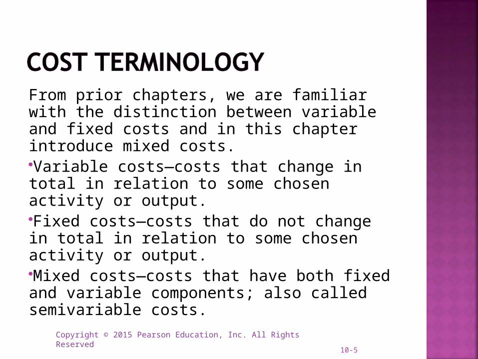
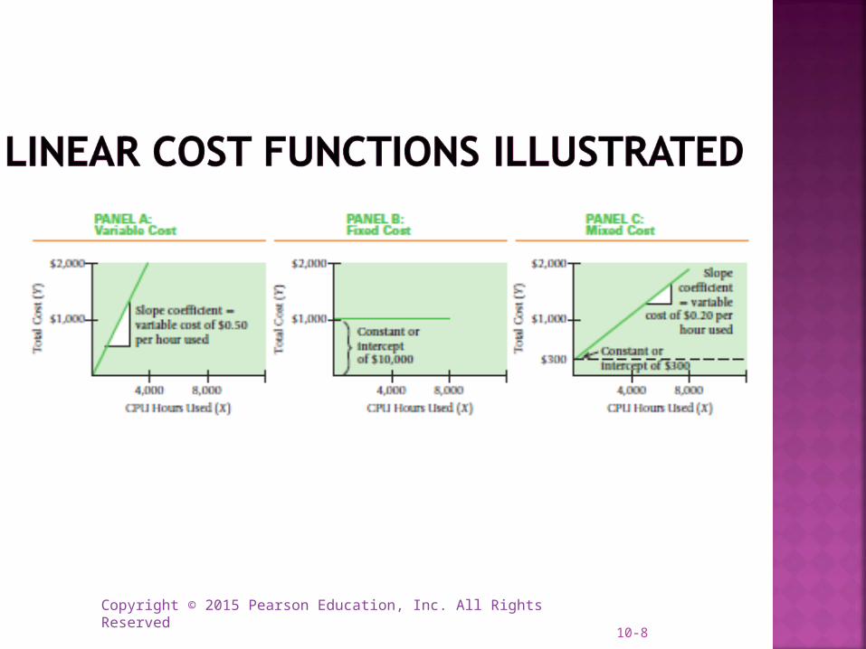
From prior chapters, we are familiar with the distinction between variable and fixed costs and in this chapter introduce mixed costs.Variable costs—costs that change in total in relation to some chosen activity or output.Fixed costs—costs that do not change in total in relation to some chosen activity or output.Mixed costs—costs that have both fixed and variable components; also called semivariable costs.
10-5
Copyright © 2015 Pearson Education, Inc. All Rights Reserved
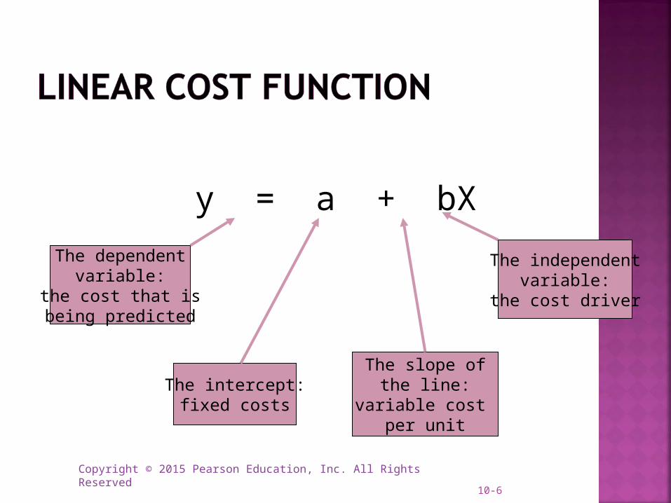
y = a + bX
The dependentvariable:
the cost that isbeing predicted
The independentvariable:
the cost driver
The intercept:fixed costs
The slope ofthe line:
variable cost per unit
10-6

Copyright © 2015 Pearson Education, Inc. All Rights Reserved
Accounting StatisticsVariable Cost Slope
Fixed Cost Intercept
Mixed Cost Linear Cost Function
10-7
Copyright © 2015 Pearson Education, Inc. All Rights Reserved10-8

Copyright © 2015 Pearson Education, Inc. All Rights Reserved
1. Choice of cost object—different objects may result in different classification of the same cost.
2. Time horizon—the longer the period, the more likely the cost will be variable.
3. Relevant range—behavior is predictable only within this band of activity.
10-9
Copyright © 2015 Pearson Education, Inc. All Rights Reserved
The most important issue in estimating a cost function is determining whether a cause-and-effect relationship exists between the level of an activity and the costs related to that level of activity.
Without a cause-and-effect relationship, managers will be less confident about their ability to estimate or predict costs.
10-10
Copyright © 2015 Pearson Education, Inc. All Rights Reserved
A cause-and-effect relationship might arise as a result of:A physical relationship between the level of
activity and the costsA contractual agreementKnowledge of operations
Note: A high correlation (connection) between activities and costs does not necessarily mean causality.
Only a cause-and-effect relationship – not merely correlation – establishes an economically plausible relationship between the level of an activity and its costs.
10-11

Copyright © 2015 Pearson Education, Inc. All Rights Reserved
To correctly identify cost drivers in order to make decisions, managers should always use a long time horizon. Managers should follow the five-step decision-making process outlined in Chapter 1 to evaluate how changes can affect costs and product decisions.
10-12
Copyright © 2015 Pearson Education, Inc. All Rights Reserved
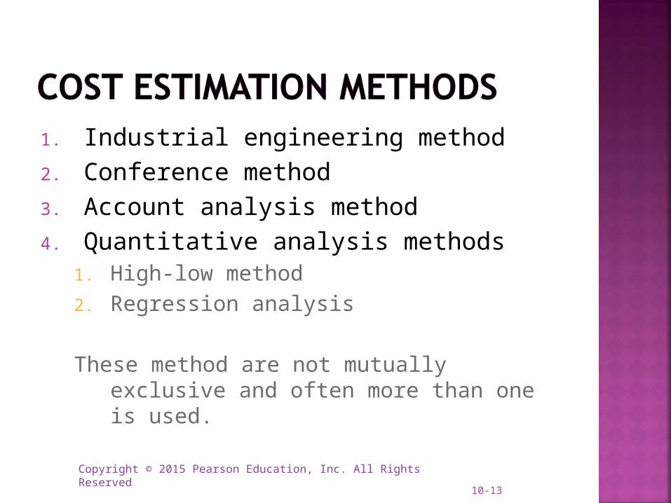
1. Industrial engineering method2. Conference method3. Account analysis method4. Quantitative analysis methods
1. High-low method2. Regression analysis
These method are not mutually exclusive and often more than one is used.
10-13
Copyright © 2015 Pearson Education, Inc. All Rights Reserved
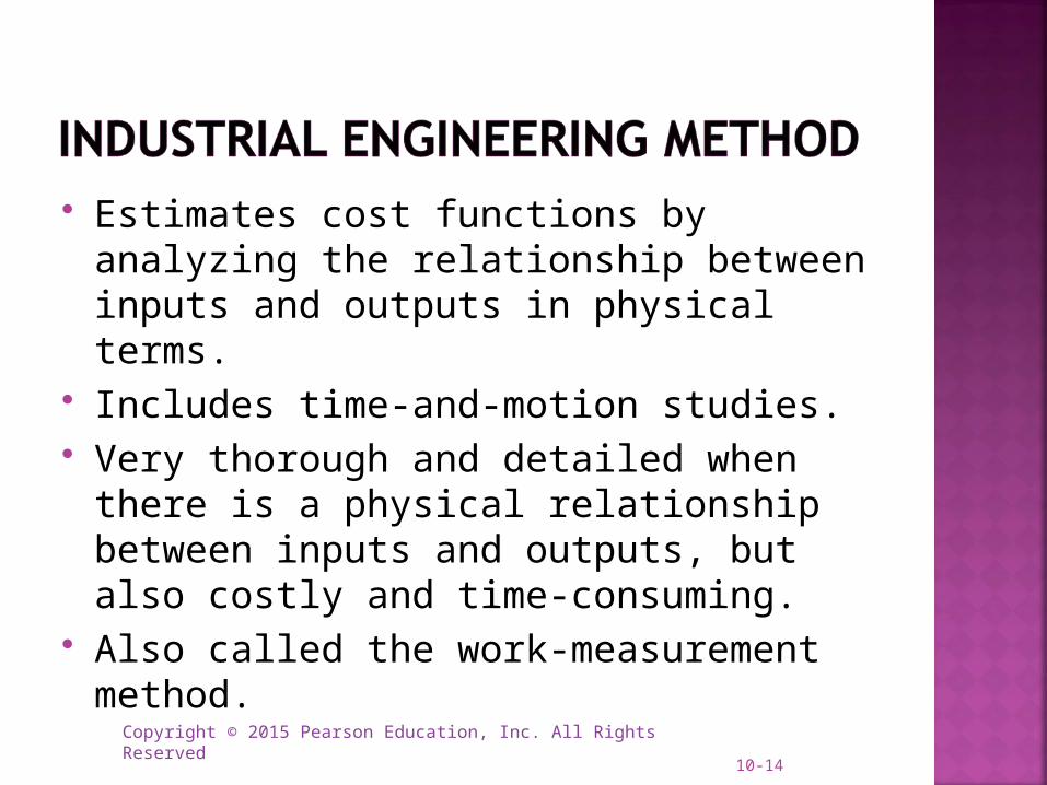
Estimates cost functions by analyzing the relationship between inputs and outputs in physical terms.
Includes time-and-motion studies. Very thorough and detailed when there
is a physical relationship between inputs and outputs, but also costly and time-consuming.
Also called the work-measurement method.
10-14

Copyright © 2015 Pearson Education, Inc. All Rights Reserved
Estimates cost functions on the basis of analysis and opinions about costs and their drivers gathered from various departments of a company.
Pools expert knowledge, increasing credibility.
Reliance on opinions makes this method subjective, though often quicker and less expensive.
10-15

Copyright © 2015 Pearson Education, Inc. All Rights Reserved
Estimates cost functions by classifying various cost accounts as variable, fixed, or mixed with respect to the identified level of activity.
Typically, managers use qualitative rather than quantitative analysis when making these cost-classification decisions.
Widely used because it is reasonably accurate, cost-effective, and easy to use, but is subjective.
10-16
Copyright © 2015 Pearson Education, Inc. All Rights Reserved
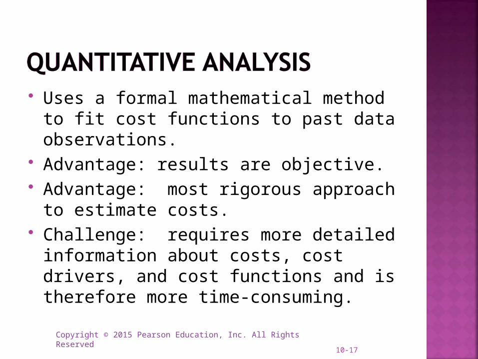
Uses a formal mathematical method to fit cost functions to past data observations.
Advantage: results are objective. Advantage: most rigorous approach to
estimate costs. Challenge: requires more detailed
information about costs, cost drivers, and cost functions and is therefore more time-consuming.
10-17
Copyright © 2015 Pearson Education, Inc. All Rights Reserved
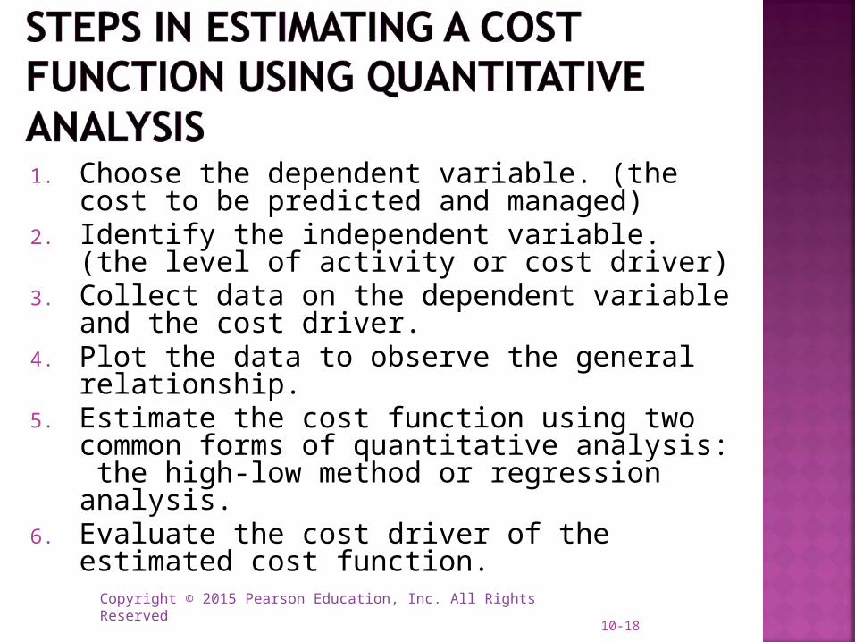
1. Choose the dependent variable. (the cost to be predicted and managed)
2. Identify the independent variable. (the level of activity or cost driver)
3. Collect data on the dependent variable and the cost driver.
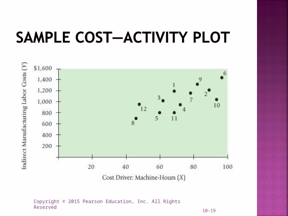
4. Plot the data to observe the general relationship.
5. Estimate the cost function using two common forms of quantitative analysis: the high-low method or regression analysis.
6. Evaluate the cost driver of the estimated cost function.
10-18
Copyright © 2015 Pearson Education, Inc. All Rights Reserved10-19

Copyright © 2015 Pearson Education, Inc. All Rights Reserved
Simplest method of quantitative analysis.
Uses only the highest and lowest observed values.
“Fits” a line to data points which can be used to predict costs.
Three steps in the high-low method to obtain the estimate of the cost function.
10-20
Copyright © 2015 Pearson Education, Inc. All Rights Reserved
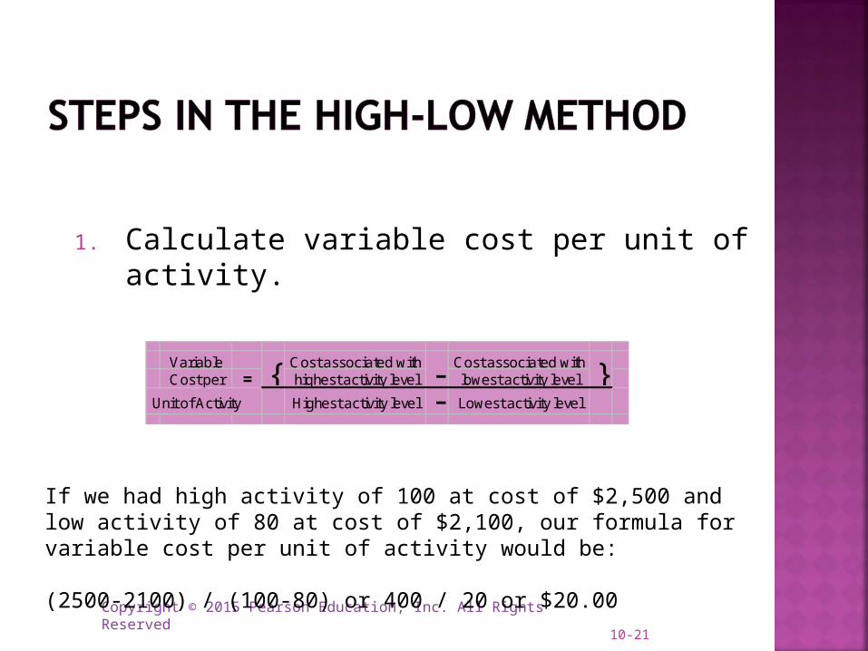
Variable Cost associated with Cost associated withCost per = highest activity level lowest activity level
Unit of Activity Highest activity level - Lowest activity level
{ - }
10-21
1. Calculate variable cost per unit of activity.
If we had high activity of 100 at cost of $2,500 and low activity of 80 at cost of $2,100, our formula for variable cost per unit of activity would be:
(2500-2100) / (100-80) or 400 / 20 or $20.00

Copyright © 2015 Pearson Education, Inc. All Rights Reserved
Total Cost from either the highest or lowest activity level- (Variable Cost per unit of activity X Activity associated with above total cost) =Fixed Costs
10-22
2. Calculate total fixed costs.
Continuing our example, let’s calculate fixed costs using both the high and low levels of activity:High- $2500 – ($20 x 100) = $500 (fixed costs)Low- $2100 – ($20 x 80) = $500 (fixed costs)

Copyright © 2015 Pearson Education, Inc. All Rights Reserved
Finally, we can summarize our calculations into the equation:Y = $500 + ($20 x X)If we wondered what costs would be at a 120 level of activity, we’ll simply plug that number for X in our equation: Y = $500 + ($20 x 120) or Y = $2,900
10-23
3. Summarize by writing a linear equation.
Y = Fixed Costs + ( Variable cost per unit of Activity * Activity )
Y = FC + (VCu * X)
Copyright © 2015 Pearson Education, Inc. All Rights Reserved
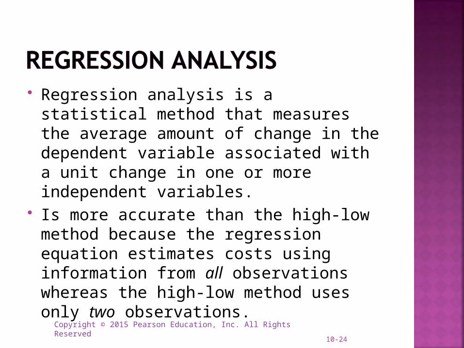
Regression analysis is a statistical method that measures the average amount of change in the dependent variable associated with a unit change in one or more independent variables.
Is more accurate than the high-low method because the regression equation estimates costs using information from all observations whereas the high-low method uses only two observations.
10-24

Copyright © 2015 Pearson Education, Inc. All Rights Reserved
Simple—estimates the relationship between the dependent variable and one independent variable.
Multiple—estimates the relationship between the dependent variable and two or more independent variables.
Regression analysis is widely used because it helps managers understand why costs behave as they do and what managers can do to influence them.
10-25
Copyright © 2015 Pearson Education, Inc. All Rights Reserved10-26
Copyright © 2015 Pearson Education, Inc. All Rights Reserved
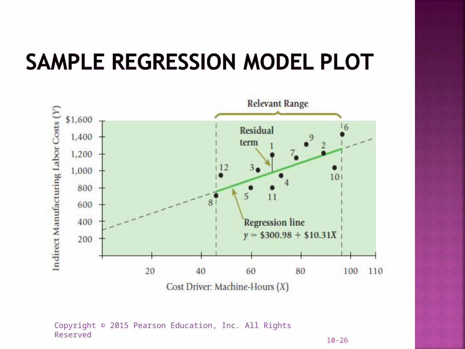
Goodness of fit—indicates the strength of the relationship between the cost driver and costs.
Residual term—measures the distance between actual cost and estimated cost for each observation. The smaller the residual term, the better is the fit between the actual cost observations and estimated costs.
10-27

Copyright © 2015 Pearson Education, Inc. All Rights Reserved
How does a company determine the best cost driver when estimating a cost function? An understanding of both operations and cost accounting is helpful. Here are the three criteria used:1.Economic plausibility2.Goodness of fit3.Significance of the independent variable.
10-28
Copyright © 2015 Pearson Education, Inc. All Rights Reserved
QUESTION: Why is choosing the correct cost driver to estimate costs important?
ANSWER: Identifying the wrong drivers or misestimating cost functions can lead management to incorrect and costly decisions along a variety of dimensions.
10-29
Copyright © 2015 Pearson Education, Inc. All Rights Reserved
Estimating cost drivers in an activity-based costing system doesn’t differ in general from what’s been discussed.However, since ABC systems have a great number and variety of cost drivers and cost pools, managers must estimate many cost relationships.They will do so using the same methods, taking special care with the cost hierarchy. If a cost is batch-level, for example, only batch-level cost drivers can be used.
10-30

Copyright © 2015 Pearson Education, Inc. All Rights Reserved
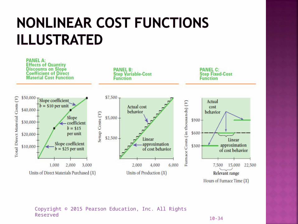
Cost functions are not always linear. A nonlinear cost function is a cost
function for which the graph of total costs is not a straight line within the relevant range.
Some examples of nonlinear cost functions follow.
10-31
Copyright © 2015 Pearson Education, Inc. All Rights Reserved
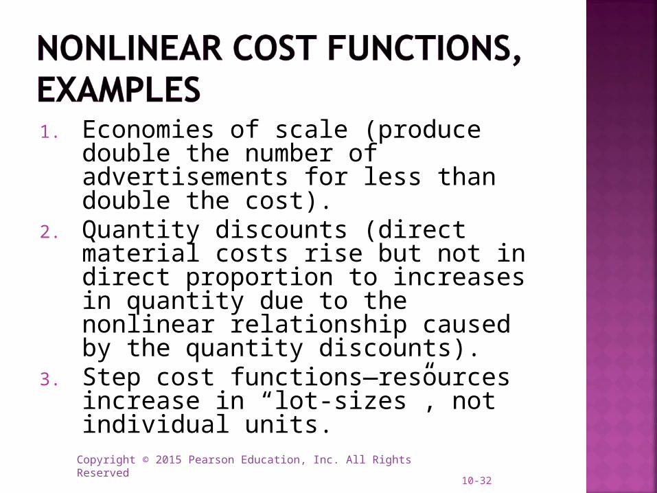
1. Economies of scale (produce double the number of advertisements for less than double the cost).
2. Quantity discounts (direct material costs rise but not in direct proportion to increases in quantity due to the nonlinear relationship caused by the quantity discounts).
3. Step cost functions—resources increase in “lot-sizes”, not individual units.
10-32

Copyright © 2015 Pearson Education, Inc. All Rights Reserved
4. Learning curve—a function that measures how labor-hours per unit decline as units of production increase because workers are learning and becoming better at their jobs.
5. Experience curve —measures the decline in the cost per unit of various business functions as the amount of these activities increases. It is a broader application of the learning curve that extends to other business functions in the value chain such as marketing, distribution and customer service.
10-33
Copyright © 2015 Pearson Education, Inc. All Rights Reserved10-34

Copyright © 2015 Pearson Education, Inc. All Rights Reserved
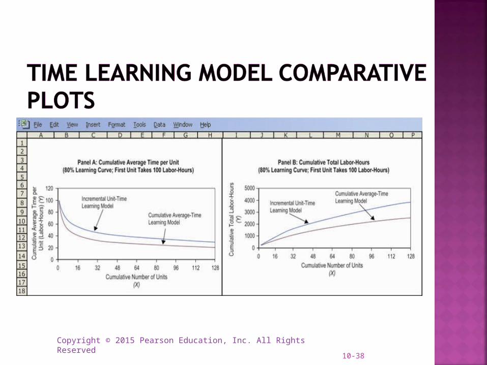
Cumulative average-time learning model—cumulative average time per unit declines by a constant percentage each time the cumulative quantity of units produced doubles.
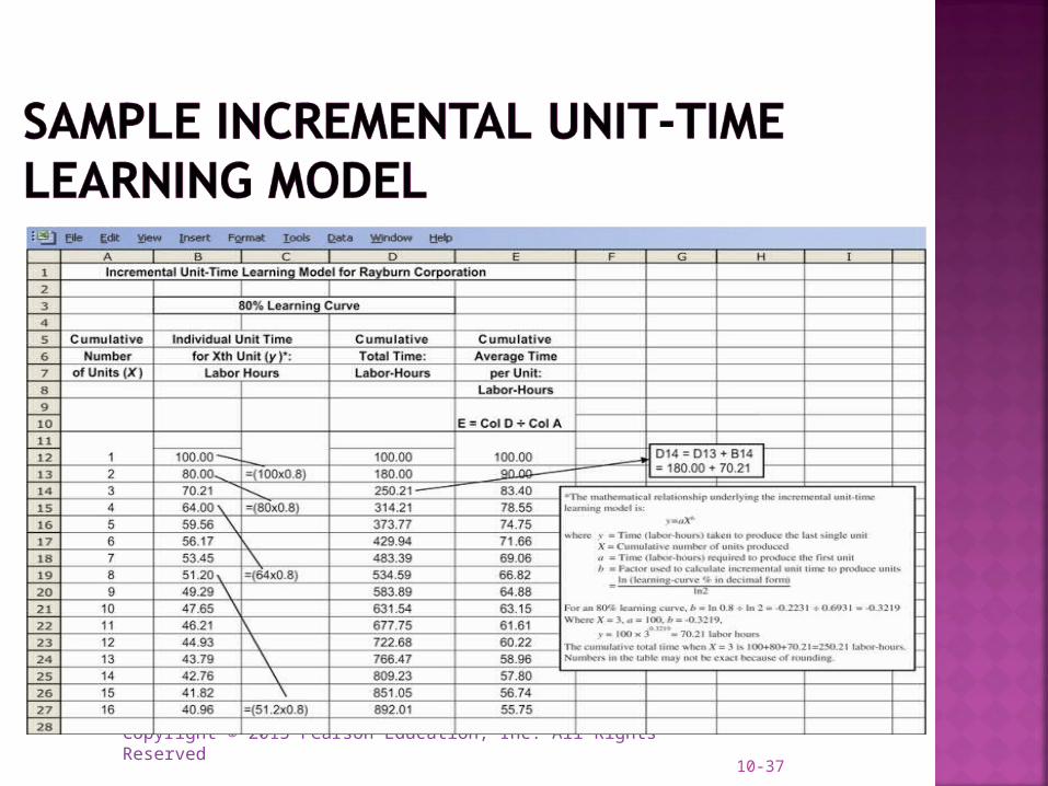
Incremental unit-time learning model—incremental time needed to produce the last unit declines by a constant percentage each time the cumulative quantity of units produced doubles.
10-35
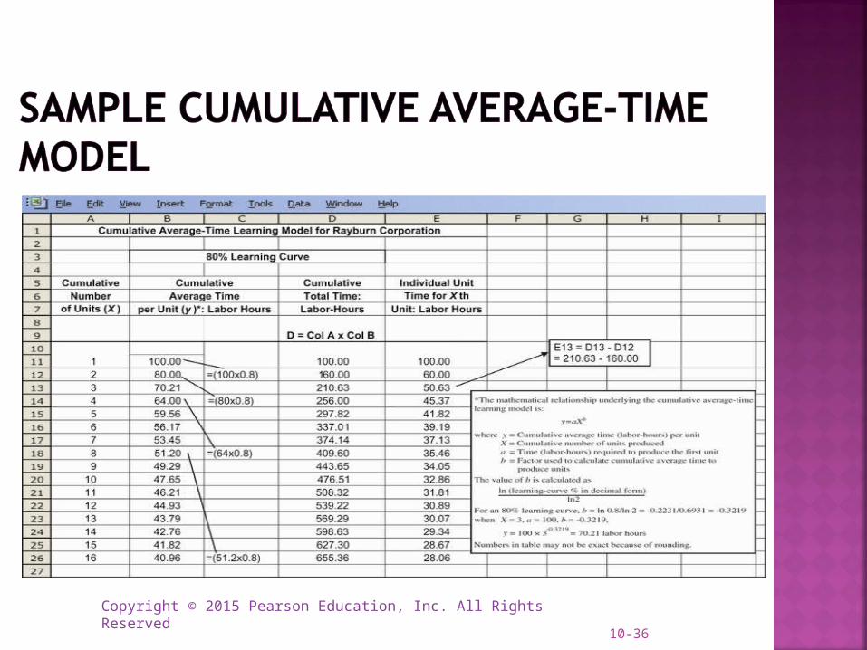
Copyright © 2015 Pearson Education, Inc. All Rights Reserved10-36
Copyright © 2015 Pearson Education, Inc. All Rights Reserved10-37
Copyright © 2015 Pearson Education, Inc. All Rights Reserved10-38

Copyright © 2015 Pearson Education, Inc. All Rights Reserved10-39
Copyright © 2015 Pearson Education, Inc. All Rights Reserved
The ideal database has two characteristics:1.The database should contain numerous reliably measured observations of the cost driver and the related costs.2.The database should consider many values spanning a wide range for the cost driver.
10-40
Copyright © 2015 Pearson Education, Inc. All Rights Reserved
1. The time period for measuring the dependent variable does not properly match the period for measuring the cost driver.
2. Fixed costs are allocated as if they are variable.
3. Data are either not available for all observations or are not uniformly reliable.
10-41

Copyright © 2015 Pearson Education, Inc. All Rights Reserved
4. Extreme values of observations occur.5. There is no homogeneous relationship
between the cost driver and the individual cost items in the dependent variable-cost pool. (A homogeneous relationship exists when each activity whose costs are included in the dependent variable has the same cost driver.)
10-42
Copyright © 2015 Pearson Education, Inc. All Rights Reserved
6. The relationship between the cost driver and the cost is not stationary. This can occur when the underlying process that generated the observations has not remained stable over time.
7. Inflation has affected the costs, the cost driver, or both.
10-43

Copyright © 2015 Pearson Education, Inc. All Rights Reserved
TERMS TO LEARN PAGE NUMBER REFERENCE
Account analysis method Page 377
Coefficient of determination Page 399
Conference method Page 377
Constant Page 372
Cost estimation Page 374
Cost function Page 371
Cost predictions Page 374
Cumulative average-time learning model
Page 390
Dependent variable Page 379
Experience curve Page 389
10-44

Copyright © 2015 Pearson Education, Inc. All Rights Reserved
TERMS TO LEARN PAGE NUMBER REFERENCE
High-low method Page 381
Incremental unit-time learning model
Page 391
Independent variable Page 379
Industrial engineering method
Page 376
Intercept Page 372
Learning curve Page 389
Linear cost function Page 371
Mixed cost Page 372
Multicollinearity Page 406
Multiple regression Page 383
10-45

Copyright © 2015 Pearson Education, Inc. All Rights Reserved
TERMS TO LEARN PAGE NUMBER REFERENCE
Nonlinear cost function Page 388
Regression analysis Page 383
Residual term Page 383
Semivariable cost Page 372
Simple regression Page 383
Slope coefficient Page 372
Specification analysis Page 401
Standard error of the estimated coefficient
Page 400
Standard error of the regression
Page 399
Step cost function Page 388
Work-measurement method Page 376 10-46

Copyright © 2015 Pearson Education, Inc. All Rights Reserved 47