copyright © 2018 by robert r. williams iii
TRANSCRIPT

Suitability Analysis for Wave Energy Farms off the Coast of Southern California: An Integrated Site Selection Methodology
by
Robert R. Williams III
A Thesis Presented to the Faculty of the USC Graduate School
University of Southern California In Partial Fulfillment of the
Requirements for the Degree Master of Science
(Geographic Information Science and Technology)
December 2018

Copyright © 2018 by Robert R. Williams III

iii
Table of Contents
List of Figures ................................................................................................................................ vi
List of Tables ............................................................................................................................... viii
Acknowledgements ........................................................................................................................ ix
List of Abbreviations ...................................................................................................................... x
Abstract ......................................................................................................................................... xii
Chapter 1 Introduction .................................................................................................................... 1
1.1. Motivation ...........................................................................................................................2
1.2. Wave Power Potential .........................................................................................................2
1.3. Benefits of Wave Energy ....................................................................................................3
1.4. Trends in Wave Energy ......................................................................................................5
1.5. Study Area ..........................................................................................................................5
1.6. Thesis Layout ......................................................................................................................6
Chapter 2 Related Work .................................................................................................................. 8
2.1. Wave Data Collection .........................................................................................................8
2.1.1. National Data Buoy Center ........................................................................................9
2.1.2. Coastal Data Information Program ..........................................................................10
2.1.3. Other Wave Data Collecting Organizations ............................................................12
2.2. Quantifying Wave Power ..................................................................................................12
2.3. Wave Energy Converter Technologies .............................................................................13
2.3.1. Categories of WEC Devices ....................................................................................14
2.3.2. Current Leading WEC Designs ...............................................................................16
2.3.3. PowerBuoy Specifications .......................................................................................17
2.4. Site Selection ....................................................................................................................18
2.4.1. Modeling Wave Power ............................................................................................18

iv
2.4.2. Assessing Limiting Factors ......................................................................................19
2.4.3. Weighted Overlay ....................................................................................................20
Chapter 3 Data and Methods......................................................................................................... 22
3.1. Research Design and Data Classification .........................................................................22
3.1.1. Research Design.......................................................................................................22
3.1.2. Data Classification ...................................................................................................23
3.2. Data Acquisition ...............................................................................................................26
3.2.1. Data Acquired for Limiting Factors .........................................................................28
3.2.2. Data Acquired for Wave Power ...............................................................................30
3.3. Methods.............................................................................................................................34
3.3.1. Data Processing ........................................................................................................34
3.3.2. Weighted Overlay ....................................................................................................50
3.3.3. Sensitivity Analysis .................................................................................................52
3.3.4. Cost-Benefit Analysis ..............................................................................................53
Chapter 4 Results and Discussion ................................................................................................. 55
4.1. Weighted Overlay Results ................................................................................................55
4.2. Sensitivity Analysis Results ..............................................................................................58
4.2.1. Breakdown of Suitability Categories .......................................................................58
4.2.2. Change in Spatial Distribution .................................................................................60
4.3. Cost Analysis ....................................................................................................................63
Chapter 5 Conclusions .................................................................................................................. 70
5.1. Limitations ........................................................................................................................71
5.2. Improvements and Future Work .......................................................................................73
References ..................................................................................................................................... 76
Appendix A. A Complete list of potential limiting factors considered by all acquired sources ... 81

v
Appendix B. Global distribution of annual mean wave power and annual mean wave direction 82
Appendix C. Map of wave power density interpolated from CDIP buoy data using the Spline with Barriers tool in ArcGIS ................................................................................................. 83
Appendix D. Detailed Return of Investment equation originally intended for the cost-benefit analysis .................................................................................................................................. 84
Appendix E: Definitions ............................................................................................................... 85

vi
List of Figures
Figure 1. Map depicting the Southern California Bight as the study area ...................................... 6
Figure 2. Diagram of wave profile with free orbital motion ........................................................... 9
Figure 3. Wave energy converter devices categorized by size and orientation to the wave ......... 14
Figure 4. Working principles of WEC devices ............................................................................. 15
Figure 5. PowerBuoy™ diagram and specifications .................................................................... 17
Figure 6. Overview of the method workflow in this study ........................................................... 23
Figure 7. Map of the average wave height for 2017 ..................................................................... 32
Figure 8. Map of the average peak wave period for 2017 ............................................................ 33
Figure 9. Map of Governmentally Regulated Areas and their suitability score ........................... 37
Figure 10. Map of Commercially Used Zones and their suitability score .................................... 39
Figure 11. Map depicting the Distance to Shore in assigned suitability scores ............................ 41
Figure 12. Map of Vessel Density in assigned suitability scores ................................................. 43
Figure 13. Map of Ocean Depth in assigned suitability scores ..................................................... 45
Figure 14. Map of Seabed Slope in assigned suitability scores .................................................... 47
Figure 15. Map depicting the distribution of wave power density with insets focusing on the limited areas with power densities greater than 25 kW/m .................................................... 49
Figure 16. Map of Wave Power Density in assigned suitability scores ........................................ 50
Figure 17. The primary wave farm suitability result .................................................................... 56
Figure 18. Category breakdown for wave farm suitability by area percentage ............................ 57
Figure 19. Sensitivity Analysis 1: Map and suitability breakdown with 40% weighted wave power ..................................................................................................................................... 59
Figure 20. Sensitivity Analysis 2: Map and suitability breakdown with 20% weighted wave power ..................................................................................................................................... 60
Figure 21. Category changes from the primary overlay (30% weight for wave power) to first sensitive analysis (40% weight for wave power) .................................................................. 61

vii
Figure 22. Category change from the primary overlay (30% weight for wave power) to second sensitive analysis (20% weight for wave power) .................................................................. 62
Figure 23. Five potential wave farm locations chosen for cost analysis ...................................... 63
Figure 24. The potential wave farm Site 1 location with primary weighted overlay ................... 64
Figure 25. The potential wave farm Site 2 location with primary weighted overlay ................... 65
Figure 26. The potential wave farm Site 3 location with primary weighted overlay ................... 66
Figure 27. The potential wave farm Site 4 location with primary weighted overlay ................... 67
Figure 28. The potential wave farm Site 5 location with primary weighted overlay ................... 68
Figure A. Global distribution of annual mean wave power .......................................................... 82
Figure B. Map of wave power density generated from CDIP buoy data using the Spline with Barriers tool in ArcGIS ......................................................................................................... 83

viii
List of Tables
Table 1. The limiting factor categories and datasets included in the wave farm suitability analysis ............................................................................................................................................... 25
Table 2. The two forms of the wave data used for calculating wave power ................................. 26
Table 3. Data types, resolutions, and sources ............................................................................... 27
Table 4. Suitability Scores used for Governmentally Regulated Areas ........................................ 35
Table 5. Suitability Scores used for Commercially Used Zones .................................................. 38
Table 6. Suitability Scores used for Distance to Shore ................................................................. 40
Table 7. Vessel Density suitability scores assignment ................................................................. 43
Table 8. Ocean Depth suitability scores assignment .................................................................... 44
Table 9. Seabed Slope suitability scores assignment .................................................................... 46
Table 10. Wave Power Density suitability scores assignment ..................................................... 48
Table 11. Weight designation of the wave farm suitability .......................................................... 51
Table 12. Weights used for Sensitivity Analysis 1 (40%) ............................................................ 53
Table 13. Weights used for Sensitivity Analysis 2 (20%) ............................................................ 53
Table 14. Cost analysis for wave farm site suitability .................................................................. 69
Table A. Complete list of potential limiting factors considered by all acquired sources ............. 81

ix
Acknowledgements
I would like to express my sincere gratitude to Dr. Wu, my advisor, for her support, guidance,
and motivation through the writing of this thesis. I’d also like to thank Dr. Bernstein for helping
me find the project that was right for me and for her encouraging words along with Dr. Vos as
my thesis committee members. Besides faculty members, I would also like to thank Corey Olfe,
a programmer/analyst for the Coastal Data Information Program, for his valuable assistance on a
crucial aspect of this project.

x
List of Abbreviations
AHP Analytic Hierarchy Process
ASBS Area of Special Biological Significance
BODC British Oceanographic Data Centre
CDFW California Department of Fish and Wildlife
CDIP Coastal Data Information Program
CF Capacity Factor
CUZ Commercially Used Zone
DEM Digital Elevation Model
EEZ Exclusive Economic Zone
EFH Essential Fish Habitat
GIS Geographic Information System
GRA Governmentally Regulated Area
GW Gigawatt
GWh Gigawatt Hour
MOP Monitoring and Prediction
MPA Marine Protected Area
MUZ Military Use Zone
NDBC National Data Buoy Center
NMS National Marine Sanctuary
NOAA National Oceanic and Atmospheric Administration
OTP Offshore Power Technology
RE Renewable Energy

xi
SA Sensitivity Analysis
SCB Southern California Bight
SWAN Simulating WAves Nearshore
TW Terawatt
TWh Terawatt Hour
WAM Wave Model
WEC Wave Energy Converter

xii
Abstract
Renewable energy is becoming increasingly important as energy prices and air pollution
increase globally. Wind and solar power have become more affordable and efficient. However,
current renewable energy production cannot bear the weight of the world’s growing need for
energy unless we can effectively tap the world’s greatest source of energy: the ocean. Wave
energy converters are technologies designed to harness the energy from the ocean waves. This
study aims to help energy resource planners identify the most efficient locations for wave farms
near the coast of Southern California. Current studies with the similar goals either only used
wave data as the variables during the decision making process or considered other variables but
omitted the wave data. Few were found to include both, yet those too are lacking in the full
scope.
In this study, wave power data as well as environmental and legal limiting factors were
included in wave farm site selection. These limiting factors, along with the wave data, consisted
of seven individual layers that were each given weights according to their importance in regards
to a PowerBuoy™ wave farm and then combined together using a weighted overlay. The results
of this overlay were used to select five areas with the most potential as a suitable location for a
wave farm. A simple cost comparison was then conducted to determine which site was the most
suitable. It was determined that a site roughly 25 kilometers due south from Point Conception
was the best candidate. However, the conditions in the sea off the coast of Southern California
are less than ideal for wave farms with the current state of wave energy conversion technology
due to a relatively low level of wave power caused by the complex geography of the region.

1
Chapter 1 Introduction
Recent environmental studies have given much attention to renewable and clean energy
due to the increasing energy demands as populations rise (Ozkop and Altas 2017). An increase in
rechargeable devices—including automobiles—is further straining the current energy supply.
Other studies focus less on local energy demands than they do on the global environmental need
of moving away from fossil fuels towards cleaner energy sources. Among the alternative energy
research, however, few studies have focused on one of the greatest untapped resources on the
planet: the ocean.
Wave energy is the combination of potential and kinetic energy harnessed from ocean
waves that is converted into electricity using wave energy converter (WEC) technologies.
Compared to solar and wind farms, the development of commercial wave farms has been slow
over the last decade. The lack of wave farms in mass production can be attributed to
technological, financial, and environmental concerns. This study aims to identify suitable
locations for wave farms with little to no commercial or environmental drawbacks. Spatial
analysis techniques in ArcGIS were used to identify such locations off the coast of Southern
California including the coastline of Santa Barbara, Ventura, Los Angeles, Orange, and San
Diego counties.
Limiting factors and wave energy are the two major considerations of wave farm site
selection. Limiting factors include any variables that might make a location inappropriate or
undesirable for the installation of a wave farm. Wave energy factors refer to the historical pattern
of the waves, primarily the average wave height and peak wave period. By using data from the
Coastal Data Information Program (CDIP), the wave patterns can be calculated for the entirety of
the study area. By combining both the limiting and wave energy factors, this study provides

2
wave energy planners with the information needed to make educated decisions early in the
planning process.
1.1. Motivation
Much of the world is turning to renewable energy (RE) sources in the face of climate
change, the depletion of non-renewable energy reserves, and a growing need for energy as the
global population continues to rise. Advancements in RE technologies continue to grow with a
14.1% increase of global energy production in 2016 coming from renewable sources including
wind, geothermal, solar, and biomass (BP 2017). Continued growth is expected in the near future
primarily in onshore wind and solar photovoltaic technologies (International Energy Agency
2016). Other contributions to this expected growth include hydropower, bioenergy for power,
offshore wind, solar thermal electricity from concentrated solar power plants, geothermal, and
ocean power. With over 40% of the world’s population living within 100 kilometers of the coast,
a concentration on ocean related RE sources could prove most beneficial (IOC/UNESCO 2011).
1.2. Wave Power Potential
Ocean power is comprised of tidal power and wave power. Theoretically, there is also
energy potential in the salinity gradient and thermal gradient of the ocean, though these
technologies have yet to progress beyond the early developmental stages. Tidal power is a form
of renewable energy which is generated from the gravitational and centrifugal forces among the
Earth, the Moon, and the Sun (Segura et al. 2017). Wave power, the focus of this study,
originates from wind energy which is then transferred to the sea surface when wind blows over
large areas of the ocean (Marine and Hydrokinetic Energy Technology Assessment Committee
2013). Although there are no commercial, grid-connected WEC technologies in the U.S.
(Lehmann et al. 2017), wave energy is estimated to be able to provide 910 terawatt hours (TWh)

3
annually for the contiguous U.S. (Lehmann et al. 2017; Electric Power Research Institute 2011).
Based on the estimate that one TWh of electricity can power 90,000 homes per year, the amount
of wave power-generated energy could power nearly 82 million homes if the full potential of
wave energy is tapped (Gosnell 2015).
1.3. Benefits of Wave Energy
Compared to other renewable resources, particularly solar and wind, wave energy is
beneficial for its predictability (several days in advance) and its consistency (throughout the day
and night). Wave energy also consists of significantly higher energy density compared to wind
and solar energy (Lehmann et al. 2017). This means that on average, more energy is available
per square meter of the ocean surface, in the form of waves, than is available per square meter of
land surface, in the form of wind or solar energy. Like these more common renewables, wave
energy is sustainable, meaning that it cannot be depleted and can be generated cleanly with no
significant harm to the environment as WECs do not produce any forms of emission (Boeker and
Van Grondelle 2011; Bento et al. 2014). However, this does not mean that wave energy
generation is completely without risks to the environment.
A major environmental concern often raised against the implementation of WECs in the
U.S. is the possibility of hydraulic fluid leaks. In response, certain WEC technologies, such as
the Pelamis, harden their mechanical components and use biodegradable fluids to minimize the
effects should a leak occur (Ilyas et al. 2014). Other environmental concerns include underwater
noise pollution and hazardous turbines, both of which could negatively affect sea life in
unpredictable ways. Fortunately, unlike designs of tidal energy converters, WECs need neither
turbines nor other noisy components.

4
On the other hand, research has also indicated wave farms as a potential line of defense
against beach erosion (Abanades, Greaves, and Iglesias 2014). Using a computer simulation
model called Simulating WAves Nearshore (SWAN), researchers identified decreases in wave
height and near-bottom orbital velocities leeward of wave farms while other wave dynamics
were generally unchanged (Chang et al. 2016). These simulated results were validated by a test
site in Lysekil, Sweden, where the reduced energy of the waves leeward of a wave farm also had
positive environmental effects. The environment was studied before and after the installment of
an array of WECs. According to this case study, 68 species were significantly more abundant in
the test site leeward of a wave farm than at the control site and no species were found to be
extinct (Ilyas et al. 2014). With this in mind, Marine Protected Areas and other conservation
areas are included as limiting factors in this suitability analysis study, but only considered to be
entirely restricted for wave farms in accordance with state or federal laws.
Besides environmental concerns, wave energy also faces opposition from commercial
interests. Current site selection methods for wave farms do not consider fishing or shipping
traffic. More than two-thirds of California’s marine fishing takes place off the coast of southern
California between the counties of San Diego and Santa Barbara. The amount of recreational
fishing alone in this region results annually in over a $2.5 billion stimulus to the state’s economy
(Southwick Associates Inc. 2009). Furthermore, shipping is one of Southern California’s most
profitable industries, with an operating revenue of 475 million U.S. dollars in Port of Los
Angeles, 355 million dollars in Port of Long Beach, and 169 million dollars in Port of San Diego
in 2016 (San Diego Board of Port Commissioners 2017; Long Beach Board of Harbor
Commissioners 2017; Los Angeles Board of Harbor Commissioners 2017).

5
The year of 2016 marked a record breaking year in terms of volume for any Western
Hemisphere port with 8.86 million containers passing through the Port of Los Angeles (Los
Angeles Board of Harbor Commissioners 2017). Following shortly behind Los Angeles in
volume was the Port of Long Beach, which handled a total of 6.78 million containers in 2016.
Together they process roughly 40 percent of all imports to the U.S. (Hricko 2006). With these
massive industries operating off of the Southern California coast, it is important to consider their
areas of operation when identifying potential wave farm locations.
1.4. Trends in Wave Energy
Wave energy has been lagging behind other RE sources due to their high cost and the
lack of an optimal design identified for commercialization (Foteinis and Tsoutsos 2017). This
uncertainty along with the constant evolution of technologies is responsible for high costs and
low commitment rates among potential investors. The current costs of wave energy exceeds
those of conventional energy generation technologies such as gas and coal (Astariz and Iglesias
2015). However, like wind energy and solar energy, the cost of wave energy will ultimately drop
as resources are no longer spent on inefficient designs but dedicated to a single WEC technology
that proves superior to all others. The foreseeable decrease of wave energy costs combined with
the potential for the rising cost of conventional energy could make wave energy an economical
option in the future.
1.5. Study Area
The study area stretches along the coast from Point Conception (~34.5°N) in the north to
San Diego and the Mexican border (~32.5 °N) in the south and westward beyond the Channel
Islands (Figure 1). This area covers over 30,000 square miles and is known as the Southern
California Bight. It is characterized by shore islands, shallow banks, and deep basins which

diminish
refraction
and Guza
1.6. Th
T
of researc
site selec
study are
The resul
of these r
towards s
deep ocean
n, diffraction
a 1993).
Figure 1
esis Layou
The remainde
ch pertaining
ction method
e introduced
lts of the stu
results in Ch
site selection
gravity wav
n, and dissip
1 Map depic
ut
er of this the
g to wave da
ds, and poten
and the met
udy’s analysi
hapter 5 alon
n, further ana
ves (Emery 1
pation resulti
cting the Sou
esis is divide
ata collection
ntial limiting
thods used to
is are provid
ng with any c
alysis will b
1960). These
ing in a spati
uthern Califo
d into four c
n, wave pow
g factors. In C
o conduct the
ded in Chapte
conclusions
e required; a
e features cau
ially comple
ornia Bight a
chapters. Cha
wer quantific
Chapter 3, th
e site selecti
er 4, which i
that were m
and though t
ause wave ref
ex wave clim
as the study a
apter 2 is a l
cation, WEC
he data requ
ion are discu
is followed b
made. As a pr
the study are
flection,
mate (O’Reill
area
literature rev
technologie
irements for
ussed in deta
by a discussi
reliminary st
ea is limited
6
ly
view
es,
r this
ail.
ion
tep
to

7
the coast of Southern California, the methods described herein can be replicated for any coast
given that the required data exists.

8
Chapter 2 Related Work
To collect wave energy as a power source, we must first understand what we intend to
capture. This literature review discusses research papers and technical reports on the most
effective means of harnessing the power of the ocean. It begins with an introduction to waves,
their attributes, and a summary of wave data collection techniques. The second section focuses
on current attempts at quantifying wave power, which is followed by a quick outline of WEC
technologies. Lastly, this review discusses the current methods of wave energy farm site
selection using nothing but the wave data. Using geographic information systems (GIS), and
including other concerning factors alongside wave data, this study ultimately extends the
research detailed in this review.
2.1. Wave Data Collection
Waves form by transferring wind energy onto the surface. This energy is measured in
kilowatts per meter of wave crest, which is referred to as wave power density (Gunn and Stock-
Williams 2012). Important wave parameters include its length (λ) and height (H). When
calculating wave energy, the depth of water (h) is also important as roughly 95% of a waves
energy exists between the surface of the water and a depth equal to a quarter of the wavelength
(Figure 2) (Ilyas et al. 2014). It is important to recognize that most waves are not simple,
harmonic or regular. Instead, the vast majority of waves are short-crested and irregular due to the
erratic nature of the wind that creates them (Electric Power Research Institute 2011).
To understand the common wave patterns of a specific ocean region for energy collection
purposes, it is important to collect massive amounts of wave data in the field. Wave data has
been collected by a number of sources over the years; this study focused on two sources that are
relevant to Southern California.

Figu
B
remainde
used to p
2.1.1. Na
T
Guard co
transferre
where it w
systems w
A
NDBC in
even in th
air and se
ure 2 Diagram
Before contin
er of Section
produce wave
ational Data
The National
onsolidated a
ed to the new
was ultimate
were deploy
As of Februar
n the coastal
he Great Lak
ea temperatu
m of wave p
nuing, it shou
n 2.1 are used
e energy. En
Buoy Cente
Data Buoy
approximate
wly formed N
ely placed un
yed, 16 of wh
ry 2018, ther
and offshor
kes (Portman
ures, wind at
rofile with f
uld be noted
d for the coll
nergy conduc
er
Center (NDB
ly 50 smalle
National Oce
nder NOAA
hich were in
re are over 1
re waters fro
nn 2016). Th
ttributes (i.e.
free orbital m
d that the tech
lection of wa
cting techno
BC) has its r
er ocean-orie
eanic and At
A’s National W
the Pacific.
100 moored
m the Pacifi
hese buoys a
. direction, s
motion (adap
hnologies de
ave data; the
ologies are co
roots in the 1
ented agenci
tmospheric A
Weather Ser
weather-oce
ic Ocean to t
are used to re
speed, and gu
pted from Bo
escribed belo
ey are not an
overed in Se
1960s when
es. In 1970,
Administrati
rvice. By 19
ean buoys de
the western A
ecord barom
ust), and wa
oström 2011
ow in the
nd cannot be
ection 2.3.
the U.S. Co
the program
ion (NOAA)
79, 26 buoy
eployed by th
Atlantic and
metric pressu
ave
9
)
e
oast
m was
)
he
d
ure,

10
measurements (i.e. significant wave height, dominant wave period, average wave period, and
wave direction).
There are four types of moored buoys currently employed by the NDBC: the 3-meter, 10-
meter, and 12-meter discus hulls, as well as the 6-meter NOMAD hulls. The larger discus buoys
are less portable and more prone to mishaps such as capsizing, while the 3-meter discus and the
NOMAD buoys are smaller and generally more durable. The choice of buoy is determined by the
deployment location and its intended purpose (National Data Buoy Center 2018).
Wave measurements are calculated for each buoy through a three-part process. First,
depending on the buoy model, the heave acceleration or vertical displacement of the hull is
measured by the accelerometer or inclinometer, respectively. Secondly, this data is converted
from the temporal domain to the frequency domain through the application of a fast Fourier
transform using an on-board processor. Lastly, this converted data is cleaned up using a response
amplitude operator process to account for electronic and hull noises. The output of these steps
includes spectral energy, significant wave height, average wave period, and dominant wave
period.
The NDBC also employs a fleet of voluntary observing ships which regularly collect and
report wind and ocean data as they conduct their usual business. There are hundreds of such
ships. Unfortunately, the majority of these ships do not report wave height or wave period,
rendering them unusable for this project.
2.1.2. Coastal Data Information Program
The Coastal Data Information Program (CDIP) began in 1975 with a single underwater
pressure sensor used to measure waves near the coast of Imperial Beach, California. With
funding from the U.S. Army Corps of Engineers, the program grew to an extensive monitoring

11
network for waves and beaches. Currently, CDIP maintains over 100 wave monitoring stations.
Though the bulk of these stations are located along the Pacific and Atlantic coasts, others are
located near the Hawaiian Islands, Guam, the Gulf of Mexico, and even in the Great Lakes
(Coastal Data Information Program 2018).
Waves are measured by CDIP using a variety of instruments. Fixed underwater sensors
include single-point gauges and arrays, both of which measure pressure fluctuations to determine
the height and period of waves passing above. A benefit of arrays is that, by linking multiple
pressure sensors together, it becomes possible to record the directional component of waves as
well. These sensors transmit the recorded data to shore using submerged cables. Surface buoys
are free of these cables as they transmit data via radio links using attached antennas, allowing
them to be deployed farther from shore. The earlier model of buoys was non-directional, though
CDIP has replaced all of these buoys with Datawell Directional Waverider buoys. This advanced
model uses a Hippy heave-pitch-roll sensor to measure wave energy attributes as well as the
wave direction.
Wave data is transferred from the various instruments to an onshore site to be stored
temporarily. This transfer occurs at a continuous interval of one to two transmissions per second.
From the onshore site, the data is then transferred to central facility twice an hour where it is
recorded, processed, and analyzed. The processing of the raw data is completed using two
FORTRAN programs. The first of these programs checks the raw data (rd) files for errors,
separates multiple sensor inputs, and calibrates the recorded values based on recorded calibration
factors before converting them into diskfarm (df) files. The second program performs a data
quality check, completes several complex calculations—such as spectral and directional wave
analyses—and produces outputs including spectral (sp) and parameter (pm) files.

12
2.1.3. Other Wave Data Collecting Organizations
Except for CDIP described in Section 2.1.2, major wave data collecting organizations do
not operate close enough to U.S. coasts to be useful for this project. One such association is the
Data Buoy Cooperation Panel, which is a joint body of the World Meteorological Organization
and the Intergovernmental Oceanographic Commission. They operate the Global
Telecommunication System, which disseminates buoy data through the World Weather Watch
with a focus on the north Atlantic (Data Buoy Cooperation Panel 2018). Other smaller
organizations are dedicated to more specific regions, such as the British Oceanographic Data
Centre and MetOcean Solutions that focus on the Southern Ocean near Antarctica. These
organizations demonstrate that buoys are the standard tool for collecting wave data around the
globe.
2.2. Quantifying Wave Power
Separate attempts to estimate the total wave energy of the world, or even just a specific
coastline, result in tremendously different numbers. This variability can be attributed to a number
of factors including differences in estimated coast lengths, wave data sources, wave attributes
considered, etc. There are no formal agreements upon the methodology for measuring this
resource.
Quantifications of the total wave power in an area represent the theoretical potential of
the area rather than the actual amount of power which could be harnessed. This wave power is
typically measured in gigawatts (GW) for areas the size of a continental coastline. Larger extents
than that might be measured in terawatts (TW, or 1,000 GW). The practical application of this
power is termed wave energy, which is measured in GW or TW per hour (GWh or TWh,

13
respectively). Many of the sources in this literature review quantify power annually (GWh/yr and
TWh/yr).
The benefits of wave energy technologies on any scale can be inferred from the global
quantifications of wave power, dated back to 1965 when Kinsman (1965) estimated 1.87 to 2.22
TW of wave power for the entire Earth. Gunn and Stock-Williams (2012) compiled a table of 11
early global wave power estimates ranging from 800 GW to 2.6 TW using three different
methods. They calculated the global nearshore wave power potential to be 2.11 TW, equal to
roughly 18,500 TWh of energy per year. Altogether, a broad extent of estimates from different
sources ranged from 16,000 TWh/yr all the way up to 32,400 TWh/yr (Reguero, Losada, and
Méndez 2015; Mørk et al. 2010).
The most recent calculation of annual global energy consumption by BP placed it at just
over 24,800 TWh for the year 2016 (BP 2017). Based on this calculation as well as the
estimation of global wave energy, ocean waves alone could meet 65 to 131 percent of the
world’s energy needs with WEC technologies at an efficiency—or capacity factor (CF)—of
100%. Unfortunately, current WEC technologies max out at a CF of 40%, which equates to a
range of only 6,400 to 12,960 TWh per year (26 to 52 percent of the global usage) (Poullikkas
2014). Still, a global array of wave farms with a 40% CF could potentially replace up to 81.5%
of the energy produced from oil and coal (BP 2017).
2.3. Wave Energy Converter Technologies
There are many WEC designs currently in use around the world, with many more being
developed every year. The number of unique WEC designs is already in the hundreds and
continues to grow as more efficient designs are invented (Khan et al. 2017).

2.3.1. Ca
C
single gro
to the wa
absorbers
through t
to a buoy
power fro
of the wa
is also a l
as a break
Figure 3
(A
T
principle
pressure
pressure
ategories of
Categorizing
oup. One me
aves (Figure
s, attenuator
the vertical m
y rising and f
om any direc
ave and gene
long device
kwater, gene
Wave energ
) Point Abso
The WEC tec
s behind the
differential,
differential p
WEC Device
these design
ethod of cate
3). By this c
rs, and termin
movement o
falling along
ction. An att
erates energy
but is positio
erating energ
gy converter
orber, (B) At
chnologies ca
em (Figure 4
floating, ov
principle inc
es
ns even prov
egorization i
categorizatio
nators (Rusu
f the devise
g the crest. It
tenuator is a
y as the wav
oned with it
gy as each w
r (WEC) dev
ttenuator, (C
an also be ca
4). There are
vertopping, a
clude those e
ves to be a ch
is by their siz
on method, th
u and Onea 2
as it rises an
t is the small
longer devic
e passes alon
s long front
wave crashes
vices categor
C) Terminato
ategorized b
four major p
and impact (L
employing th
hallenge as m
ze and direc
here are thre
2017). A poi
nd falls with
lest WEC ty
ce oriented h
ng the length
facing the d
s into the dev
rized by size
or (adapted f
by dividing th
principles re
López et al.
he Archimed
many do not
ction of the d
ee main WE
int absorber
the passing
ype and can c
horizontally
h of the devi
direction of th
vice.
e and orienta
from López e
he devices b
egarding WE
2013). Devi
des effect an
t easily fit in
device in rela
C types: poi
generates en
waves, simi
capture wave
in the direct
ise. A termin
he wave and
ation to the w
et al. 2013)
by the physic
EC design:
ices utilizing
nd those
14
nto a
ation
int
nergy
ilar
e
tion
nator
d acts
wave:
c
g the

operating
troughs a
and can b
of the str
waves. L
impact. T
some tha
T
deploym
at which
waters cl
just beyo
shore wh
common
Terminat
and less p
type devi
g with oscilla
and crests. F
be single or m
ructure, forci
Lastly, impac
There are oth
at fit into mu
Figure 4 Wo
The third met
ent. There ar
the device i
losest to shor
ond that at ab
here the wate
one being d
tors, howeve
predictable w
ices.
ating water c
loating struc
multi-part de
ing the water
ct devices are
her devices t
ultiple catego
orking princ
thod of categ
re three grou
s designed to
re where the
bout 10-25 m
ers are over 4
deployed and
er, are uncom
wave directi
columns, bot
ctures are tho
evices. Over
r to flow thr
e positioned
that do not fa
ories depend
ciples of WE
gorizing WE
ups in this ca
o be located
e waters are r
meters deep;
40 meters de
d can include
mmon in nea
ons near the
th relying on
ose that gene
rtopping dev
rough turbine
d against the
all within an
ing on the co
EC devices (a
EC technolog
ategorization
. Onshore en
roughly 1-10
offshore con
eep (Khan et
e point absor
arshore locat
e coastline. O
n pressure di
erate energy
vices rely on
es as the wat
wave front i
ny of these fo
omplexity o
adapted from
gies is by the
n using the c
nergy conver
0 meters dee
nverters are
t al. 2017). O
rbers, attenu
tions because
Onshore devi
ifferences be
y through osc
n waves crash
ter level dro
in order to ab
our categorie
f the design.
m López et a
eir proximity
correspondin
rters are tho
ep; near-shor
typically the
Offshore dev
uators, and te
e of the shor
ices are near
etween wave
cillatory mot
hing over the
ops between
bsorb the wa
es and there
.
al. 2013)
y to shore up
ng water dep
se located in
re converters
e farthest fro
vices are the
erminators a
rter wavelen
rly all termin
15
e
tions
e top
ave’s
are
pon
pths
n
s are
om
most
like.
ngths
nator

16
2.3.2. Current Leading WEC Designs
Of the hundreds of current WEC designs, relatively few have made it beyond the research
and development phase. Moreover, fewer designs have been deployed to actively generate
energy other than for testing purposes. The Pelamis attenuator, originally manufactured by
Pelamis Wave Power (now made by Wave Energy Scotland), is among those well-established
designs. The world’s first commercially active wave farm was a Pelamis wave farm, completed
off the coast of Portugal in July 2008 (Poullikkas 2014). Other Pelamis wave farms have since
gone into operation in the coastal waters of England as well as Scotland. There are currently no
real contending attenuator designs to the Pelamis though there are few in the field testing stage.
As for terminator devices, there have been a couple commercially active designs since the
late 1990s. For example, Oceanlinx deployed a blueWAVE terminator in Australian waters and
Wavegen deployed one of their LIMPET systems off the coast of the United Kingdom. These
onshore designs have since gained competition by Wave Dragon ApS in Denmark (Rusu and
Onea 2017). Prior to the Pelamis attenuator becoming the first commercial wave farm, in 2003
the Wave Dragon became the world’s first offshore grid-connected WEC, though it only
produced local, non-commercial energy (Peter et al. 2006).
None of the aforementioned WEC designs have a solid footing in the U.S. despite
multiple attempts to do so over the last two decades (Wang, Isberg, and Tedeschi 2018).
However, the U.S. has been actively involved in the field of wave energy conversion during this
period. By 2009, the U.S. already boasted more WEC concepts than any other country, though
not more than Europe as a whole (López et al. 2013). Currently, the only design with plans for
commercial use in the U.S. is the PowerBuoy™, a point absorber, by a New Jersey based
company called Offshore Power Technology (OTP). Because of this being the only commercial

wave farm
project.
2.3.3. Po
T
The Pow
two main
falls in re
motion d
converted
and Edw
as well a
F
m in the plan
owerBuoy Sp
The design an
werBuoy™ ca
n component
eaction to th
drives a push
d into a rotar
ards 2014).
s the moorin
Figure 5 Pow
nning stages
pecifications
nd specificat
an be describ
ts of the desi
e waves whi
h rod connect
ry action by
The table in
ng system an
werBuoy™ d
s in the U.S.,
tions of the P
bed as a two
ign—the flo
ile the heave
ted to the flo
a mechanica
the right sid
nd electrical
diagram and
, the PowerB
PowerBuoy™
o-body floati
at and the he
e plate resists
oat into the s
al actuator to
de of Figure
specification
specification
Buoy was sel
™ is briefly
ing point abs
eave plate (F
s the pull of
spar where th
o drive an el
5 describes
ns.
ns (Mekhich
lected as the
reviewed in
sorber. This
Figure 5). Th
f the float. Th
his linear mo
lectric gener
the dimensi
he and Edwa
e focus for th
n this subsect
means there
he float rises
his relative
otion is
rator (Mekhi
ons of the de
ards 2014)
17
his
tion.
e are
s and
iche
evice

18
2.4. Site Selection
Selecting suitable locations for wave farms requires the calculation of wave power
potential for the study area as well as a careful consideration of all factors which would limit
where a wave farm could be placed.
2.4.1. Modeling Wave Power
Wave power modeling relies on three wave parameters: wave height, peak wave period,
and mean direction of the wave (Gunn and Stock-Williams 2012). As mentioned in Section 2.1,
the height and length of waves relate directly to the potential wave power. The directional
component is a diffusing factor in that wave energy is generally stronger as it flows
perpendicular into a shoreline and weaker in the lee of an obstacle. Another diffusing factor is
the ocean depth which comes into effect in shallow waters as swell energy, from deep ocean
waves, dissipates due to bottom friction and refraction (Wilson and Beyene 2007).
Current wave energy studies rely heavily on wave modeling software that are free of cost.
The leading free software for wave modeling is Simulating WAves Nearshore (SWAN), which
predicts the growth, decay, and transformation of waves given a set of input physical and
environmental parameters (Sørensen et al. 2004). SWAN is a “third generation” wave model that
takes into account whitecapping, wave-on-wave interactions, and bottom dissipation (in
comparison of those “second generation” models considering only wave interactions). SWAN is
unique in including wave-on-wave interactions between three waves as well as depth-induced
wave breaking (Booij, Ris, and Holthuijsen 1999). Wave conditions are simulated in the SWAN
model using user-input data including the local wind speed and direction, bathymetry, and water
boundary. Results of this model are then validated using hindcast data (or backtesting using
historical data) as a basis of comparison. In the Southern California Bight (SCB), the validation

19
results of SWAN are typically accurate to about 0.13 meters, with a higher level of error in
shallower waters (Rogers et al. 2007; Gorrell et al. 2011).
The Coastal Data Information Program (CDIP) has a wave model called the Monitoring
and Prediction (MOP) system which is used to monitor and provide current wave conditions to
the public. MOP is a buoy-driven wave model using hindcast data collected from an array of
deployed buoys in combination with a wave propagation model to generate wave predictions
(O’Reilly et al. 2016). The MOP system generates three standard products: regional swell
predictions, inner water sea and swell predictions, and alongshore sea and swell predictions.
With expert knowledge on the system, MOP was designed specifically with the complex
bathymetry of the SCB in mind. Hindcast validation of this model shows similar errors as those
occurring in wind-wave generation and propagation models such as SWAN.
Other wave modeling software exists. Two examples are the Wave Model Development
and Implementation Group’s WAve Model (WAM) and NOAA’s Wavewatch III. Both are third-
generation wave models similar to SWAN, but they do not perform as well in validation despite
WAM being the first of its kind (Rogers et al. 2007). Alternative model options such as
Aquaveo’s Coastal Wave Modeling with SMS model developed by the U.S. Army Corp of
Engineers offer more customer friendly interfaces available at a steep price.
2.4.2. Assessing Limiting Factors
While wave power is the leading factor in wave farm suitability, a site with optimal wave
conditions is only suitable if it is not restricted for use due to legal regulations, current ocean
uses, or technical limitations. Legal regulations include laws that prohibit activities affecting
natural habitats in the environmentally sensitive areas. Marine Protected Areas, for example, are
areas restricting activities for purposes of maintaining biodiversity (Nobre et al. 2009). Areas of

20
international economic exclusivity fall into this group. Certain human activities currently
occurring in nearshore ocean waters are also likely to influence where a wave farm can or cannot
be placed. Commonly cited limiting factors include oil and gas extraction, military activities,
shipping routes, fisheries, and submarine cables and pipelines (Zubiate et al. 2005).
Lastly, WEC devices are designed to be deployed and operate in specific conditions.
These technical specifications physically limit where wave farm can be placed based on water
depth and seabed slope (Vasileiou, Loukogeorgaki, and Vagiona 2017). A complete list of
limiting factors considered for wave farm installations can be found in Appendix A.
2.4.3. Weighted Overlay
Research regarding weighted overlays was conducted specifically for those focusing on
wave farm site selection. Possible weights for the layers of limiting factors and wave power were
identified through this literature review, providing a range of weighting systems which could be
implemented, and each with their own merit. Two sources in particular referenced wave power
as a factor in wave site selection.
Vasileiou et al. (2017) gave wave power a weight of 29.2% with other factors including
water depth (15%), distance from shore (5%), and vessel density (3.2%). However, this source
also used factors such as wind velocity, connection to electrical grid, and population served that
were not considered for this study. Wind velocity was given a score of 29.2%, equal that of wave
power since this site selection study was for a hybrid wave energy and wind energy farm.
Vasileiou’s site selection process included an analytic hierarchy process (AHP) with pairwise
comparison of the factors to determine these weights, a process requiring an official survey to
acquire advanced knowledge from a number of experts.
21
A second source, again using an array of different factors in their AHP, assigned wave
power a weight of 31.5% (Ghosh et al. 2016). This value was actually the sum of two separate
categories, wave height and distance between waves, which are essentially the two factors of
wave power. Ocean depth (7.9%) and vessel density (4.8%) were also considered in this study.
Other factors included water quality, coastal erosion, tourism potential, and more. These factors,
and the others, were not considered as they are either difficult to measure, impossible to score, or
irrelevant for this study.

22
Chapter 3 Data and Methods
This chapter lists the datasets and the sources of the data used in this study. It also
discusses the methods employed to use this data to identify the most suitable locations off the
coast of Southern California where wave farms can be installed with the least environmental,
commercial, and social impacts. The identified suitable locations were analyzed for their cost-
benefit ratio so that interested parties can have a greater scope of knowledge when selecting
potential suitable sites for wave farm installations.
3.1. Research Design and Data Classification
3.1.1. Research Design
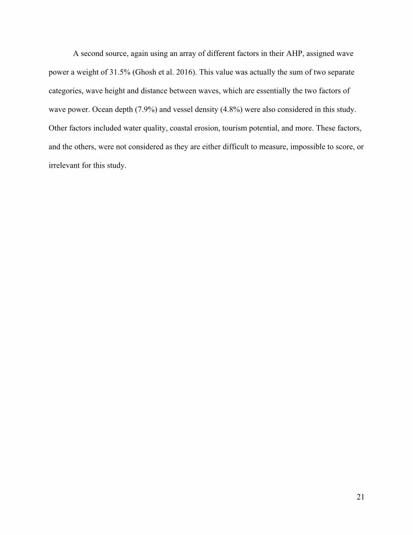
The design of this project is summarized in the workflow depicted in Figure 6. It begins
with the acquisition of pre-processed data from various sources. This data is then processed
separately for vector and raster data types, though with similar steps and identical results. This
process includes scoring the data on a one to five (1-5) suitability scale, followed by a process to
ensure that each dataset has the same extent boundaries, and ends by converting each into
uniform raster datasets of equal extent and cell size. Once this is complete, all data is input into a
final output of a single weighted overlay. This process will be discussed in depth in the following
sections.
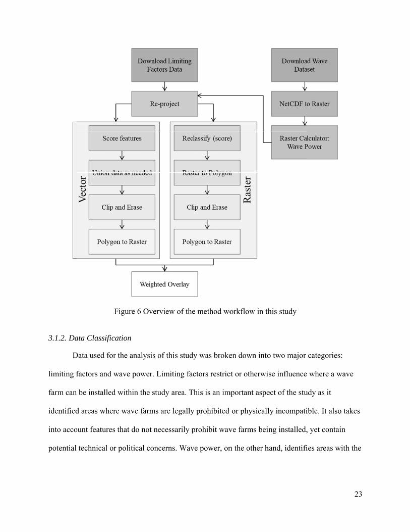
3.1.2. Da
D
limiting f
farm can
identified
into acco
potential
F
ata Classific
Data used for
factors and w
be installed
d areas wher
ount features
technical or
Figure 6 Ove
ation
r the analysis
wave power.
d within the s
re wave farm
that do not
r political co
erview of th
s of this stud
. Limiting fa
study area. T
ms are legally
necessarily p
oncerns. Wav
e method wo
dy was broke
actors restric
This is an im
y prohibited
prohibit wav
ve power, on
orkflow in th
en down into
ct or otherwi
mportant aspe
or physicall
ve farms bein
n the other h
his study
o two major
se influence
ect of the stu
ly incompati
ng installed,
hand, identifi
categories:
e where a wa
udy as it
ible. It also t
, yet contain
ies areas wit
23
ave
takes
n
th the

24
most and least potential power. It acts as a foundation for the study, which is supplemented by
the limiting factors to narrow down the most suitable wave farm locations.
The limiting factors were categorized into six classes, as listed in Table 1 below. Out of
the six classes, three represent areas limited by laws and current uses:
I. Governmentally Regulated Areas (GRA): This class includes all regions where a
city, state, federal, or military law regulates marine usage;
II. Commercially Used Zones (CUZ): This class includes the regions of significant
commercial use;
III. Vessel Density: Vessel density symbolizes the concentration of annual vessel
traffic.
These next three classes are self-explanatory and represent areas limited by the physical terrain
and distance to shore that influences the cost or effectiveness of the technology:
IV. Ocean Depth
V. Seabed Slope
VI. Distance to Shore

Table 1 T
T
including
included
gravel ex
available
fishing in
The limiting
There were m
g kelp beds,
as they fell
xtraction site
e for the stud
n the SCB is
g factor categ
more limiting
eelgrass bed
within the re
es and dredgi
dy area. Fish
not limited
gories and da
g factors con
ds, aquacultu
egions alread
ing locations
eries dataset
to any speci
atasets inclu
nsidered but n
ure farms, div
dy restricted
s were not in
ts were anoth
ific areas as
uded in the w
not included
ve sites, and
d due to shall
ncluded as th
her factor th
well as the f
wave farm su
d in this stud
d surf spots,
low water de
his data was
hat was not in
fact that ava
uitability ana
dy. Such fact
were not
epth. Sand a
not readily
ncluded as
ilable fishin
25
alysis
tors,
and
g

numbers
regards to
is difficu
distances
L
identify w
As shown
wave hei
power.
3.2. Da
D
Details a
are generali
o scale. Last
ult to quantify
s from shore
Limiting the l
where wave
n in Table 2
ight and peak
Table 2 T
ta Acquisi
Data for this p
bout the sou
ized by large
tly, attitudin
fy. Instead, a
where wave
location of a
farms would
, the factors
k wave perio
The two form
ition
project was
urce data and
e grid square
al factors su
a simple rang
e farms wou
a wave farm
d be most ef
necessary to
od. Together
ms of the wa
acquired fro
d their acquis
es presenting
uch as public
ge of buffers
ld be most li
is only half
ffective aside
o determine
r, these varia
ave data used
om five diffe
sitions are d
g a modifiab
c opinions w
s in Class VI
ikely to be v
of the proce
e from conce
the wave po
ables can be
d for calcula
erent sources
described in t
le areal unit
ere not inclu
I was used to
visible to the
ess. Wave po
erns about li
ower of an ar
used to calc
ating wave p
s as listed in
the following
problem in
uded as this d
o represent s
e public.
ower was use
imiting facto
rea comprise
culate wave
ower
Table 3 belo
g sections.
26
data
hort
ed to
ors.
e
ow.

Table 3 Data types, resolutionns, and sourcces
27

28
3.2.1. Data Acquired for Limiting Factors
Marine Protected Areas (MPA) and Areas of Special Biological Significance (ASBS)
were provided by the California Department of Fish and Wildlife (CDFW), both of which were
polygon features downloaded as individual shapefiles that were ready to use. Most of the
datasets, however, was acquired from National Oceanic and Atmospheric Administration
(NOAA), which vetted and uploaded data from various original sources. The polygon vector
datasets from NOAA, according to Table 3, required no formatting and were ready to use.
However, oil platforms, as points, and submarine cables and oil pipelines, as lines, required an
additional step after download before they could be processed for analysis.
The additional step required for point and line features was to create polygon buffers at
significant distances. For the oil platforms, two buffers were created: a 500-meter buffer
representing the rigs’ minimum safety distance in accordance with standard safety practices and
a larger one-kilometer buffer representing the area of increased rig-related vessel traffic. There
were no found regulations regarding the minimum safety buffers for pipelines and submarine
cables; however, a similar study for wave farm suitability analysis used 500 meters for this
buffer distance, matching those of the oil platforms applied in this study (Nobre et al. 2009).
Following that example, a 500-meter buffer was used here as well. These buffers were used in
lieu of their corresponding points and lines in the data processing step.
These vector datasets contained no metadata about source accuracy. When possible,
randomly selected features within each dataset were manually confirmed according to
coordinates on official documents or through satellite imagery. MPAs, for example, are each
described in detail with exact coordinates in title 14, section 632 of the California Code of
Regulations (2017). Similarly, National Marine Sanctuaries (NMS) were confirmed from the
Code of Federal Regulations (2009), title 15, sec. 9.922, which provides a general description of

29
the boundaries along with exact coordinates. Other legal or political boundaries could not be as
easily confirmed, though any error would be expected to be relatively minor at the scale of this
study. Oil platforms were the only features that could be visually confirmed. On the other hand,
oil pipelines and submarine cables could not be fully verified. A small level of verification for
these features was achieved by the fact that their beginning and end points aligned properly with
verifiable locations such as power stations and oil platforms.
Vessel density data was acquired through NOAA as a raster dataset. It was collected by
the U.S. Coast Guard for any vessel equipped with an Automatic Identification Systems (AIS)
transponder. AIS transponders are required, according to Regulation 19.2.4 of the International
Maritime Organization’s Safety of Life at Sea (SOLAS) convention, for all internationally
voyaging ships of 300 gross tonnage or more, non-internationally voyaging ships of 500 gross
tonnage or more, and passenger ships of any size (International Maritime Organization 2007).
The transponder sends GPS coordinates, among other data, every two to ten seconds with a
positional accuracy of 0.0001 minutes. The National Oceanic and Atmospheric Administration
(NOAA) and the Bureau of Ocean Energy Management (BOEM) jointly compiled this data into
a raster with 100-meter grid squares for the contiguous United States offshore waters.
The bathymetry data was acquired as a single raster from BODC, a British agency with a
global bathymetry database compiled in 2014. This source was chosen for its large areal extent
and relatively high raster resolution (30 arc seconds) in comparison to other sources with similar
coverage. 30 arc seconds equates to an approximate raster cell size of 30.9 x 25.7 meters at the
latitude of the SCB. While this raster file was ready to be used for the ocean depth requirement,
it was also processed to create the seabed slope layer using the Slope tool in ArcGIS.
30
Lastly, the distance to shore feature was creating using the buffer tool on a shapefile of
the 2017 version of California counties acquired from the U.S. Census Bureau. The county
polygons were first dissolved into a single feature and all islands were removed before the
buffers were created. Buffers were set at 1, 2.5, 5, 50, 75, 100, and 150 kilometers according to a
logical combination of the values suggested from multiple sources (Nobre et al. 2009; Vasileiou,
Loukogeorgaki, and Vagiona 2017).
All limiting factor datasets acquired were the most up-to-date versions available and were
representative of the actual features at the time of the analysis (July 2018), with a single
exception. Vessel density described the vessel traffic patterns during the year of 2013. This is
acceptable, as it represents a historical trend rather than strict legal boundaries, meaning that
more recent data would not necessarily predict future vessel density any more accurately than
data from 2013.
3.2.2. Data Acquired for Wave Power
To create the wave power layer, a NetCDF file containing the raster layers of the average
wave height and the average peak wave period for the year of 2017 was acquired from CDIP.
The NetCDF file was created by the team at UC San Diego’s Scripps Institute of Oceanography
(Scripps) on request. While the two raster layers could have been generated by the wave models
using the Monitoring and Prediction (MOP) computer program, there were some technical
limitations of installing the MOP program on my personal computer. The request was given with
specific parameters for the study area as well as the timeframe for the entire year of 2017 for
which the wave data was to be averaged. Rather than an average of a 9-band energy spectra,
which is ideal for nearshore waves, the averages of wave height and peak wave period were
acquired so that it could be used to more accurately model the waves farther offshore.

31
While a request like this was happily fulfilled by a team of experts, it is important to
understand how the model used for generating the wave data was created. The program used to
create these wave models is MOP v1.1, downloadable from the CDIP code access webpage
(cdip.ucsd.edu/code_access). The system requirements include a FORTRAN compiler and
NetCDF4 packages. The Scripps team recommends using a Linux operating system and provides
installation instructions in the MOP download package. With knowledge of FORTAN compilers,
MOP can be installed on most modern computer systems.
Running a model in MOP is a two-step process: first, define output sites; and second,
create “hindcast predictions” or wave models for that defined site. Defining the output site can be
done through R_CA_nc, the first of two tools found within the MOP program. The input values
of this tool are the decimal degree coordinates of the CDIP wave data gathering buoys that were
selected for the analysis. Next, follow the coordinates with a five-digit site designation, ideally a
meaningful prefix followed by the buoy number. An example command would be “%
./R_CA_nc 32.93045 -117.39239 BP100”. Running this code results in a NetCDF site definition
file that will be used in step two. This should be repeated for each selected buoy.
The second step of running a wave model uses the second of the tools found in the MOP
program, the net_model. This tool has many different parameters that allow for customization.
The first parameter is the start time (-s), input as 2017010100 for the start of the year 2017. Next
is the duration parameter (-h); it can be set for an hour, week, or month. There is a workaround to
run this model for longer periods, such as for an entire year, which was necessary for this study.
To do this, a new parameter (-z) would be included followed by OWI_hc. This allows the model
to be run with multiple start times while the output NetCDF file is appended rather than rewritten
each time. The next parameter required is the NetCDF site definition files (-c) created in step

one. The
that exten
to connec
to acquir
“% ./net_
socal_alo
options g
R
raster dat
ArcGIS w
Figure 8)
initializatio
nds the near
ct to the THR
re and store t
_model -s 20
ongshore_hin
given coastal
Running the t
tasets. This i
was used to
).
n parameter
shore param
REDDS serv
the data on th
017010100 -
ndcast.INPU
l bathymetry
two-step pro
is what the S
export the im
Figure 7 M
s file name (
meters. The fi
ver to load th
he local mac
h m -c BP10
UT -z OWI_h
y of a differe
ocess above r
Scripps team
mbedded wa
Map of the a
(-i) comes ne
inal paramet
he buoy data
chine. An ex
00_32.93045
hc -e -O”; ho
ent study are
results in the
m provided. T
ave data laye
average wav
ext, followed
ter, another f
a via openda
xample comm
5-117.39239
owever, ther
a.
e NetCDF fi
The Make Ne
ers into raste
ve height for
d by a flag c
flag comman
ap. This elim
mand would
9_ref.nc -i
re are a num
le containing
etCDF Raste
er datasets (s
2017
command (-e
nd (-O), is u
minates the ne
d look like th
mber of other
g the require
er Layer too
ee Figure 7
32
e)
sed
eed
his:
ed
ol in
and

F
combined
height an
where P r
to gravity
tool in A
“WaveH
temperatu
gradient
or the two w
d to create a
nd peak wave
represents w
y (ms-2), H i
ArcGIS was u
eight” * “W
ure and salin
is considere
Figure 8 Ma
wave data lay
single wave
e period usin
wave power (
is wave heig
used for this
WavePeriod”)
nity over a sp
d very limite
ap of the ave
yers to be us
e power data
ng the follow
𝑃
(W/m), p rep
ght (m), and
calculation:
. While wate
pan of the oc
ed. Thus, a v
erage peak w
seful for this
aset. Wave p
wing formula
𝑝𝑔64𝜋
𝐻 𝑇
presents wat
T is peak wa
(1025 * 9.8
er density ca
cean, in a lim
value of 102
wave period f
project, the
power can be
a:
er density (k
ave period (
8 * 9.8) / (64
an fluctuate d
mited area li
5 kg/m3 was
for 2017
two raster la
e calculated f
kgm-3), g is
s). The Rast
4 * 3.14) * (“
due to the va
ike the SCB,
s given (Fran
ayers were
from wave
acceleration
ter Calculato
“WaveHeigh
ariations of w
, the density
nzi et al. 201
33
n due
or
ht” *
water
16).

34
The remaining values in this equation are for acceleration due to gravity at 9.8 m/s2 and pi which
was rounded down to 3.14. The cell values of the resulting raster dataset represent the mean
wave power in Watts per meter of wave crest, or wave power density.
3.3. Methods
The analysis of this study consists of two major steps: (1) Process the data in preparation
of an overlay and (2) conduct a weighted overlay analysis to produce the final data output. This
section breaks down both of these steps so that the study can be replicated for other study areas.
All geoprocessing tasks and spatial analyses—except where noted—were completed using
ESRI’s ArcGIS for Desktop version 10.4.1 running on a Windows 10 laptop with 16 GB of
RAM.
3.3.1. Data Processing
The purpose of this first step is to prepare every dataset to have the same projection,
extent, and cell size, ensuring the best results in the weighted overlay. All of the vector and raster
datasets were first assigned the same coordinate system—the California Teale Albers projection
with the North American Datum of 1983 (NAD 1983 California Teale Albers)—using the
Project tool from the Data Management toolbox in ArcGIS. A projected coordinate system was
required for accurate areal measurements.
Next, a scoring system for the weighted overlay was established. Each individual feature
would be given a suitability score of a value one through five, with one (1) being least suitable
and five (5) being the most suitable for wave farm installations. A logical scoring technique was
used to score each feature based on their limitations according to the sources referenced. Aside
from these features, others were given a restricted score of zero (0) due to technical limitations or
legal regulations which completely remove these areas from consideration.

3.3.1.1. V
In
Table 4 l
(GRA):
The reaso
Vector Datas
n this study,
lists the summ
Table
oning of the
Marin
any an
may o
theref
Areas
though
place
within
restric
sets
the limiting
mary of the
4 Suitability
above score
ne Protected
nd all comm
operate in the
for all MPAs
of Special B
h many proh
to protect th
n ecosystems
ctions, a scor
factor datas
scores used
y Scores used
es in GRA fo
Areas (MPA
mercial activit
ese areas, wh
s were given
Biological S
hibit dredgin
he most biolo
s sensitive to
re of two (2)
sets were spl
for the first
d for Govern
or the individ
A) are federa
ties. Only ce
hich does no
n a restricted
ignificance (
ng and other
ogically sign
o outside dis
) was given t
lit into six cl
class, Gover
nmentally Re
dual layers i
al and state p
ertain preapp
ot fit the desc
score of zer
(ASBS) are
seabed alter
nificant regio
sturbances. W
to these feat
lasses (see S
rnmentally R
egulated Are
is provided b
protected are
proved resea
cription of a
ro (0).
not as prote
ring activitie
ons, much of
Without stri
tures.
Section 3.1.2
Regulated A
eas
below:
eas which fo
arch operatio
a wave farm
cted legally,
es. They are
f which occu
ct legal
35
).
Areas
orbid
ons
,
in
ur

36
National Marine Sanctuaries (NMS) have the widest range of area and many
MPA and ASBS fall within the extent of these sanctuaries. There are two NMS
within the study area: Channel Islands NMS and Cordell Bank. Both regulate the
uses of these areas for educational and research purposes as well as to protect
maritime heritage and high-risk species. There are, however, no regulations
prohibiting wave farms given that the proper protocols and permits are provided.
For this reason, NMS were given a suitability score of three (3).
Essential Fish Habitats (EFH) are areas designated by NOAA as fisheries to help
increase the region’s fish population. As evident by their boxlike extents, these
areas do not strictly represent any habitats, but are placed at strategic locations
according to the species of fish being protected. Wave farms would pose little to
risk for these fish, though interest groups might protest given that the technology
is largely unproven. Therefore a suitability score of four (4) was given to these
features.
Mexico Exclusive Economic Zone (EEZ) is the maritime limit of Mexico’s legal
claim to economic resources. U.S. based wave farms would face jurisdictional and
bureaucratic issues, earning this feature a suitability score of one (1).
Military Use Zones are designated by the U.S. Air Force and Navy as dangerous
due to military activities. Exact regulations pertaining to the legality of wave
farms within these extents are unknown, but it was logically determined that they
would be considered restricted as well, thus a score of zero (0) was assigned to
them.

A
with the
layers wa
(GRA) u
by the Un
ensure th
merged w
represent
a score o
the mainl
to be use
A new attribu
appropriate
as dissolved
sing the Uni
nion tool. Th
he same exte
with that sam
ting the area
f five (5). La
land as well
d in further
Figure 9 M
ute field calle
suitability sc
into a single
ion tool. Are
his dataset w
nt used for a
me extent box
as where no l
astly, a land
as the island
analysis. Fig
Map of Gove
ed “suitabili
core using th
e feature bef
eas of overla
was then clip
all datasets in
x polygon, a
limiting fact
feature poly
ds of Califor
gure 9 depict
ernmentally R
ty” was crea
he Field Calc
fore being m
apping featur
ped to the ar
n the weight
again with th
or was prese
ygon dataset
rnia was use
ts the final o
Regulated A
ated in each
culator. Onc
merged into a
res had mult
rea of an ext
ted overlay.
he Union too
ent within th
t from the U.
d to elimina
outcome of th
Areas and the
layer and wa
ce scored, ea
a single datas
tiple scores a
tent box poly
Then the da
ol, to create a
he study area
.S. Census B
ate all areas a
his process.
eir suitability
as populated
ach of the six
set for Class
assigned to t
ygon, create
ataset was
a feature lay
a, and was gi
Bureau inclu
above sea lev
y score
37
d
x
s I
them
d to
yer
iven
ding
vel

C
manner a
The reaso
Commercially
as the GRE (
Tab
oning for the
Shipp
at the
strictly
Oil Pl
due to
the tw
(0). A
emerg
call, a
Oil Pi
water
this pa
y Used Zone
(Table 5).
ble 5 Suitabi
e scores assi
ing Lanes ar
ports of Los
y prohibited
latforms hav
o the length o
wo. Wave far
A larger buffe
gency related
a suitability s
ipelines requ
but also alo
ath and was
es (CUZ), Cl
ility Scores u
gned in the i
re designated
s Angeles an
d, making a r
ve a required
of the oil pla
rms would b
er of one kilo
d safety zone
score of thre
uire regular c
ng the sea fl
given a suita
lass II of the
used for Com
individual la
d in- and out
nd Long Bea
restricted sco
500-meter s
atform’s anc
e equally at
ometer was
e. This buffe
ee (3) was ch
checks and m
loor. A 500-m
ability score
e limiting fac
mmercially U
ayers is as fo
t-bound lane
ach. Obstruct
ore of zero (0
safety buffer
hor cables a
risk thus the
also include
er is less rest
hosen.
maintenance
meter buffer
e of one (1).
ctors, was sc
Used Zones
ollows:
es for vessel
ting these la
0) the only o
r for any anc
and possible
ey were scor
ed to represen
trictive and,
making a cl
r was chosen
cored in a sim
traffic dock
anes of traffic
option.
choring vess
contact betw
red as restric
nt a larger
in a judgme
lear path abo
n to represen
38
milar
king
c is
els
ween
cted
ent
ove
nt

L
the Union
restrictio
from this
T
IV and V
broken d
two prim
Subm
the sa
featur
Like the GRE
n tool. They
ns which wa
s dataset as w
Figure 1
The final vect
V) are in raste
own into the
mary consider
marine Cables
ame buffer di
res.
E dataset, the
y were also jo
as given a su
well. Figure
10 Map of C
tor layer is C
er format an
e five catego
rations when
s, like oil pip
istance and s
ese CUZ fea
oined with th
uitability sco
10 shows th
Commercially
Class IV, Dis
nd will be dis
ories as descr
n creating an
pelines, requ
suitability sc
atures were d
he extent box
ore of five (5
he final outco
y Used Zone
stance to Sh
scussed in th
ribed in Tab
nd scoring th
uire regular c
core of one (
dissolved and
x to represen
5). The areas
ome of this p
es and their
hore. All rem
he next sectio
ble 6. Econom
hese buffers
checks and m
(1) were give
d then merge
nt areas free
s above sea l
process.
suitability sc
maining datas
on. Distance
mics and aes
distance to t
maintenance
en to those
ed together u
e from
evel were er
core
sets (classes
e to Shore w
sthetics are t
the coastline
39
so
using
rased
III,
as
the
e.

T
shoreline
kilometer
that dista
shore, the
suitability
kilometer
ranges w
50 kilom
suitable f
A
experienc
strictly p
to the coa
farm with
for some
score of t
The economic
e and the pot
rs was given
ance to shore
e cost for ca
y scale. The
rs and betwe
were given th
meters from th
for the cable
As for the aes
ces due to w
rohibit wave
astline) were
hin a kilome
recreational
two (2) was
Table 6 Su
c concern is
tential wave
n for a score
e would be v
ble infrastru
cost for cab
een 50 to 75
e suitability
he shoreline
e cost, and th
sthetics conc
wave farms b
e farm placem
e scored as r
eter of the sh
l concerns si
assigned for
uitability Sco
in regards to
farm locatio
of one (1) fo
very costly. B
ucture is still
ble infrastruc
kilometers t
scores of th
, except whe
herefore earn
cern, it invol
eing seen as
ment, no ran
restricted (0)
horeline wou
ince many hu
r the distanc
ores used for
o the cost of
on. For these
for the least s
Between the
on the high
cture for the
to shore—be
hree (3) and f
ere aesthetic
ning the max
lves the pote
s eyesores. S
nges of dista
) or even the
uld be highly
uman activit
e of one kilo
r Distance to
f cable per k
e reasons, an
suitability, c
distance of
end so it sco
next two ran
ecomes mod
four (4), resp
s come into
ximum score
ential negativ
Since unpleas
ance to huma
least suitab
y contested fo
ties occur in
ometer to sho
o Shore
kilometer bet
ny location b
onsidering a
100 and 150
ored a two (
nges—betwe
derately econ
pectively. An
play, is con
e of five (5) i
ve impacts o
sant aestheti
an developm
le (1). Howe
for visual aes
n region. Thu
ore in this ca
tween the
beyond 150
anything bey
0 kilometers
2) on the
een 75 to 10
nomical, so t
nywhere bel
sidered the m
in this class.
on human
ics would no
ment (in this c
ever, a wave
sthetic as we
us, a suitabil
ategory. Fro
40
yond
to
00
these
low
most
ot
case,
e
ell as
ity
m

there, the
given to t
range bet
considere
except th
A
Shore da
the raster
datasets.
In
layers us
e farther offs
the range be
tween 2.5 an
ed beyond th
he ranges me
After the suit
taset was cli
r dataset usin
Figure 11 sh
Figure 11
n preparation
ing the Poly
shore, the hig
etween 1 and
nd 5 kilomet
he range of r
entioned abo
ability score
ipped to the
ng the same
hows the fin
Map depicti
n of the weig
ygon to Raste
gher the suit
d 2.5 kilomet
ers. The dist
recreational a
ve for the ec
es were appli
study area e
approach m
nal outcome o
ing the Dista
ghted overla
er tool from
tability score
ters to shore
tance to shor
activities and
conomic con
ied to the ap
extent. The a
mentioned as
of this reclas
ance to Shore
ay, these vect
the Convers
e would get.
e and a score
re greater tha
d therefore w
ncerns.
ppropriate va
areas above s
that for both
ssified suitab
e in assigned
tor datasets w
sion Tools to
A score of t
e of four (4) w
an 5 kilomet
was given a
alue range, th
sea level wer
h the GRA a
bility for Dis
d suitability
were conver
oolbox in Ar
three (3) was
was given to
ters was
score of five
his Distance
re removed f
and CUZ
stance to Sh
scores
rted into rast
rcGIS. Each
41
s
o the
e (5),
to
from
hore.
ter

42
dataset was converted individually, but with identical parameters as follows. For each, the
suitability score was selected as the Value field, the Cell Assignment Type was left with the
default CELL_CENTER, the Cellsize was set to 100 (meters), and no Priority field was selected.
3.3.1.2. Raster Datasets Preparation
The process of preparing the raster datasets was more complicated than working with
vector datasets. Because the raster datasets acquired are floating type rasters that naturally do not
contain attribute information, the process of assigning suitability scores was completed through
reclassifying each raster into an integer type raster with the desired classification. The Reclassify
tool in the Spatial Analyst extension in ArcGIS was used to perform this task.
Vessel Density, Class III of the limiting factors in this study (See Section 3.1.2),
represents the density of boat traffic for 2013. According to the metadata of this raster layer, the
cell values for the dataset do not represent the actual number of vessels and should be treated as a
high-low density scale. These values were classified into five suitability score categories using
the Standard Deviation classification method in ArcGIS. The Interval Size was set to “1 Std
Dev” resulting in four value ranges of one standard deviation. Those areas in the highest vessel
density range were given a score of one (1) and those that fell into the category with the lowest
density were given a score of four (4). Suitability scores of two (2) and three (3) were given to
the two categories falling in between. The areas absent of vessel density values were assigned a
score of five (5). Table 7 lists the range of the values and their assigned scores.

O
layer usin
vector da
Figure 12
Once reclassi
ng the Raste
atasets of clip
2 shows the
Fig
Table 7 Ve
ified, the Ve
er to Polygon
pping to the
final output
ure 12 Map
essel Density
ssel Density
n tool in Arc
extent polyg
of this vesse
of Vessel D
y suitability
y raster layer
cGIS. From t
gon and eras
el density lay
Density in ass
scores assig
r was conver
there, the sam
sing the land
yer.
signed suitab
gnment
rted into a po
me procedur
d features wa
bility scores
olygon featu
re applied to
as completed
43
ure
o the
d.

O
Digital E
economic
PowerBu
this techn
and corre
A
operating
therefore
however,
made to a
as the on
meters to
a depth r
energy po
Ocean Depth
Elevation Mo
cs. Because
uoy™, the oc
nology (Mek
esponding sc
According to
g depth rang
e assigned a
, were assign
account for g
ngoing maint
o 500 meters
ange betwee
otential is m
, Class IV of
odel (DEM)
the only WE
cean depth s
khiche and E
cores.
Table 8 O
the manufac
ing between
suitability sc
ned a score o
greater depth
tenance, the
s—were give
en 100 meter
met. This rang
f the limiting
and was sco
EC technolog
suitability wa
Edwards 201
Ocean Depth
cturer’s spec
n 25 meters a
core of zero
of one (1) as
hs. Due to th
next two cat
en the suitab
rs and 250 m
ge was given
g factors (Se
ored based on
gy currently
as categorize
4). Table 8 s
h suitability s
cifications, th
and one kilom
(0) for restri
s the source a
he increases
tegories—50
bility scores o
meters, a bala
n a suitabilit
ee Section 3.
n two factor
y planned for
ed based on
shows this b
scores assign
he PowerBu
meter. Depth
icted. Depth
also notes th
in the initial
00 meters to
of two (2) an
ance between
ty score of fo
.1.2), was re
rs: WEC cap
r installation
the recomm
breakdown o
nment
uoy™ design
hs below 25
hs beyond on
hat costly adj
l cost of inst
one kilomet
nd three (3),
n cost and e
our (4), reser
classified fro
abilities and
n in the U.S.
mendations fo
of depth rang
n has an
meters were
ne kilometer,
justments ca
tallation as w
ter and 250
respectively
stimated wa
rving the sco
44
om a
d
is
or
ges
e
,
an be
well
y. At
ave
ore
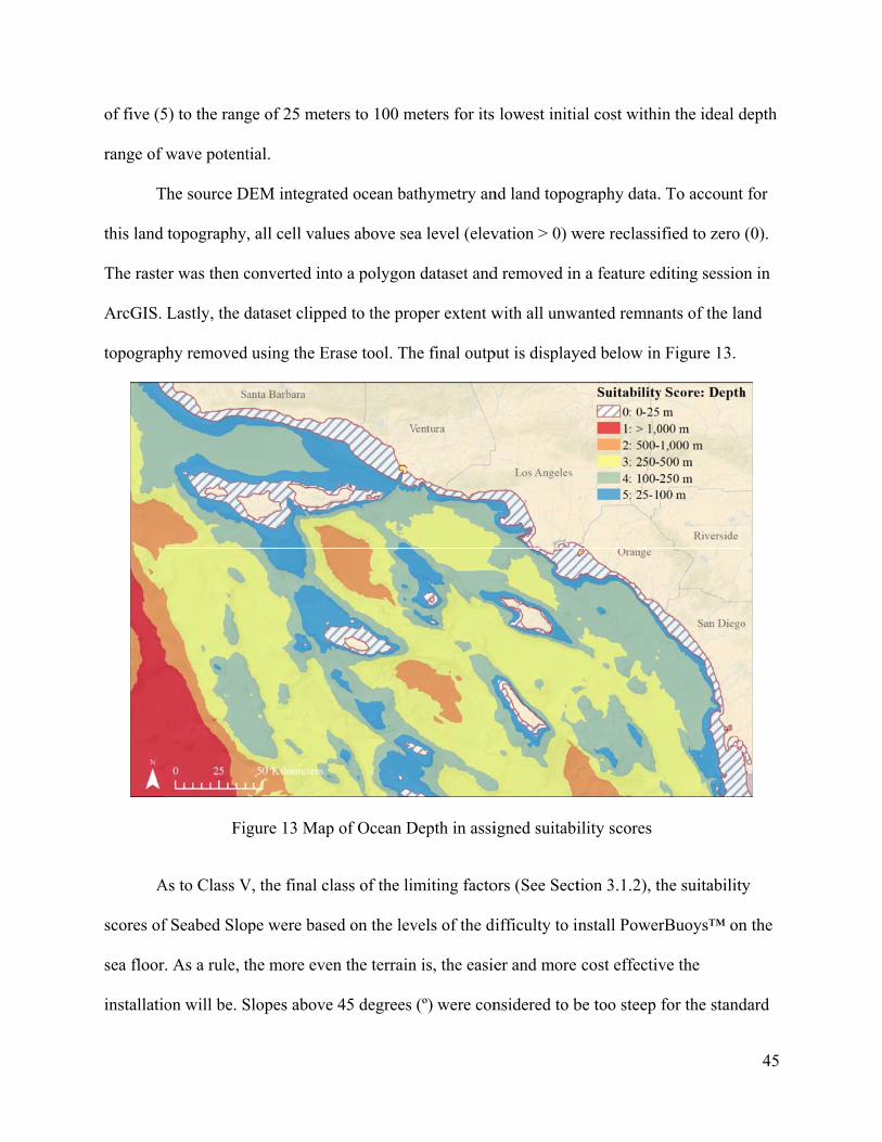
of five (5
range of
T
this land
The raste
ArcGIS.
topograp
A
scores of
sea floor
installatio
5) to the rang
wave potent
The source D
topography,
er was then c
Lastly, the d
hy removed
Fig
As to Class V
f Seabed Slo
. As a rule, t
on will be. S
ge of 25 met
tial.
DEM integrat
, all cell valu
converted int
dataset clipp
using the Er
gure 13 Map
V, the final cl
pe were base
the more eve
Slopes above
ters to 100 m
ted ocean ba
ues above se
to a polygon
ed to the pro
rase tool. Th
p of Ocean D
lass of the li
ed on the lev
en the terrain
e 45 degrees
meters for its
athymetry an
ea level (elev
n dataset and
oper extent w
he final outp
Depth in assi
imiting facto
vels of the di
n is, the easie
(º) were con
lowest initia
nd land topog
vation > 0) w
d removed in
with all unw
put is display
igned suitabi
ors (See Sect
ifficulty to i
er and more
nsidered to b
al cost withi
graphy data.
were reclassi
n a feature ed
wanted remna
yed below in
ility scores
tion 3.1.2), t
install Power
cost effectiv
be too steep
in the ideal d
. To account
ified to zero
diting sessio
ants of the la
n Figure 13.
the suitability
rBuoys™ on
ve the
for the stand
45
depth
t for
(0).
on in
and
y
n the
dard
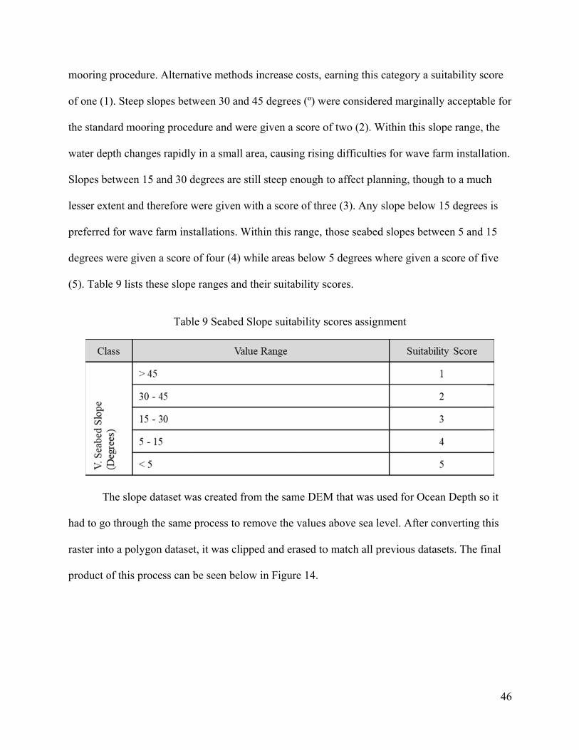
mooring
of one (1
the stand
water dep
Slopes be
lesser ext
preferred
degrees w
(5). Tabl
T
had to go
raster int
product o
procedure. A
). Steep slop
dard mooring
pth changes
etween 15 an
tent and ther
d for wave fa
were given a
e 9 lists thes
The slope dat
o through the
o a polygon
of this proce
Alternative m
pes between
g procedure a
rapidly in a
nd 30 degree
refore were g
arm installati
a score of fou
se slope rang
Table 9 S
taset was cre
e same proce
dataset, it w
ss can be see
methods incr
30 and 45 d
and were giv
small area, c
es are still st
given with a
ions. Within
ur (4) while
ges and their
eabed Slope
eated from th
ess to remov
was clipped a
en below in
rease costs, e
degrees (º) w
ven a score o
causing risin
teep enough
a score of thr
n this range,
areas below
r suitability s
e suitability s
he same DEM
ve the values
and erased to
Figure 14.
earning this
were consider
of two (2). W
ng difficultie
to affect pla
ree (3). Any
those seabed
w 5 degrees w
scores.
scores assign
M that was u
s above sea l
o match all p
category a s
red marginal
Within this sl
es for wave f
anning, thoug
slope below
d slopes betw
where given
nment
used for Oce
level. After c
previous data
suitability sc
lly acceptabl
lope range, t
farm installa
gh to a much
w 15 degrees
ween 5 and 1
a score of fi
ean Depth so
converting th
asets. The fin
46
core
le for
the
ation.
h
is
15
ve
o it
his
nal

T
convert e
were con
each, the
with the
selected.
It
layers int
were fou
were recl
when retu
Fig
The final step
each back int
nverted using
suitability s
default CEL
Once comp
t is importan
to polygons
nd to be acc
lassified into
urning the fe
gure 14 Map
p in preparin
to raster form
g the Polygo
score was se
LL_CENTER
leted, all six
nt to note tha
and then bac
eptable for t
o discrete va
eature to rast
p of Seabed S
ng the datase
mat. Like the
n to Raster t
lected as the
R, the Cellsiz
x classes had
at the potenti
ck into raste
three reasons
alues. Two, th
ter layers thu
Slope in assi
ts in this sec
e original ve
tool with the
e Value field
ze was set to
d the same co
ial for errors
rs was caref
s. One, this p
he CELL_C
us preservin
igned suitab
ction for the
ector layers f
e same input
d, the Cell A
o 100 (meter
oordinate sys
s occurring fr
fully conside
process was
CENTER cel
ng the discret
ility scores
weighted ov
from Section
t parameters.
ssignment T
rs), and no P
stem, extent
from the conv
ered. The pot
performed a
l assignment
te values. An
verlay was to
n 3.3.1.1, the
. Recall that
Type was left
Priority field
t, and cell siz
version of ra
tential errors
after the laye
t type was u
nd three, at a
47
o
ese
for
ft
was
ze.
aster
s
ers
used
a cell

size of 10
original c
3.3.1.3. W
W
since the
to the stu
regions o
kW/m in
value as t
and divid
T
three ran
scores of
density w
density v
grouping
00 meters, an
cell sizes. At
Wave Power
Wave Power
values vary
udy area, the
outside of the
the SCB, m
the upper lim
ded into five
Ta
The values be
ge from 5 to
f two (2), thr
was comprise
values above
gs on the win
ny shift of c
t such a scal
r Dataset Pre
Density was
y dramaticall
suitability s
e SCB. Whil
more than 99%
mit, an adjus
categories,
able 10 Wav
elow 5 kW/m
o 10 kW/m, 1
ree (3), and f
ed those of 2
25 kW/m. T
ndward side
ells to align
e, the maxim
eparation
s treated diff
ly by region.
scoring syste
le the highes
% of the wav
sted mean fo
each with a
ve Power Den
m were score
10 to 15 kW
four (4), resp
20 kW/m and
These high w
of the two w
to the new e
mum shift of
ferently than
Because the
em would no
st values of w
ve power de
or the wave p
5 kW/m ran
nsity suitabi
ed a one (1)
W/m, and 15 t
pectively. Th
d above, inc
wave power
western most
extent were w
f less than 50
n other datas
e range of w
ot be general
wave power
nsity was be
power densit
nge (Table 10
ility scores a
for least suit
to 20 kW/m
he last suitab
luding some
density valu
t islands in b
within the er
0 meters is n
ets in this su
wave power d
lly applicabl
r density wer
elow 25 kW/
ty in this reg
0).
assignment
tability. From
were given
bility class o
e cells with h
ues existed o
both the nort
rror limits of
negligible.
uitability ana
density is un
le for most
re greater tha
/m. Using th
gion was obt
m there, the
the suitabilit
of wave pow
high wave po
only in small
thern and
48
f the
alysis
nique
an 50
hat
ained
next
ty
er
ower

southern
class. No
analyses.
Figure
T
calculate
to the pro
The suita
chain of isla
ote that the v
.
e 15 Map de
l
The process o
d wave pow
oper extent a
ability score
ands within t
values depict
epicting the d
limited areas
of converting
wer data (see
and any area
map of wav
the SCB (Fig
ted are for re
distribution o
s with power
g the raster i
Section 3.3.
as overlappin
ve power can
gure 15) and
eference purp
of wave pow
r densities gr
into polygon
.1.2). The ne
ng land featu
n be seen in F
d were not g
poses only a
wer density w
reater than 2
n was perform
ewly created
ures were eli
Figure 16.
iven a separ
and were not
with insets fo
25 kW/m
med with the
d polygon fea
minated from
rate suitabilit
t used in any
ocusing on th
e previously
ature was cli
m the featur
49
ty
y
he
y
ipped
e.

T
Density v
input par
for the w
3.3.2. We
T
wave pow
Weighted
weighted
B
weighted
Figure
The final step
vector datase
rameters use
weighted over
eighted Over
The Weighted
wer in order
d Overlay to
d according t
Both sources
d overlay wh
e 16 Map of W
p in preparat
et back into
d for the pre
rlay had the
rlay
d Overlay w
to determin
ool uses a com
to its importa
cited in the
hich were not
Wave Power
ion of the w
raster forma
evious six da
same coordi
was the metho
e areas of hi
mmon meas
ance.
literature rev
t used in this
r Density in
weighted over
at using the P
atasets. Once
inate system
od chosen to
igh and low
surement sca
view in Chap
s study and w
assigned su
rlay was to c
Polygon to R
e completed,
m, extent, and
o combine th
suitability fo
ale to overlay
apter 2 had ad
were lacking
uitability sco
convert the W
Raster tool w
, all seven da
d cell size.
he limiting fa
or wave farm
y multiple ra
dditional lay
g other layer
res
Wave Power
with the same
atasets prepa
actors and m
ms. The
asters each
yers in their
rs which wer
50
r
e
ared
mean
re

included
from thes
research
A
importan
remainin
of how d
as they re
failure of
which are
project. T
offers an
the lowes
automati
instance,
. This made
se sources an
for this proj
T
As with the o
nce than othe
ng values wer
depth affects
epresent the
f such projec
e not as pres
Tied at 10%
y legal restri
st weighted l
cally restrict
which is a m
a one-to-one
nd logical co
ect, a fair tab
Table 11 We
other studies
er factors, thu
re closer in w
the effective
legal and pu
cts. Next, Di
ssing as high
each are the
ictions or mu
layer is the C
ted. Only the
minor overal
e comparison
onclusions b
ble of weigh
eight designa
mentioned,
us Wave Pow
weight, with
eness of the
ublic concern
istance to Sh
her weighted
e Vessel Den
uch risk of in
CUZ at 8% d
e extended o
ll concern.
n of the weig
based on pers
hts was deve
ation of the w
wave power
wer Density
h Ocean Dep
WECs. This
ns, both of w
hore was wei
d factors, but
nsity and Sea
ncreasing in
due to the fa
one-kilomete
ghts imposs
sonal knowle
eloped (Table
wave farm su
r was determ
y was assigne
pth outweigh
s was follow
which play a
ighted 12% d
t can still com
abed Slope l
nstallation co
act that most
er buffer is b
ible. Howev
edge acquire
e 11).
uitability
mined to hold
ed a weight
hing them all
wed by the G
a major role i
due to econo
mplicate fina
layers, neithe
osts beyond b
features wit
being weighe
ver, borrowin
ed through
d far more
of 30%. The
l at 16% bec
GRA layer at
in the succes
omic concern
ancing for a
er of which
budget. Last
thin the laye
ed in this
51
ng
e
cause
14%
ss or
ns,
tly,
er are

52
These layers and values were entered into the Weighted Overlay tool in ArcGIS. The “1
to 5 by 1” Evaluation scale was selected so that it would match the Suitability Score scale of 1
through 5. This automatically filled in the Scale Value field to match the Field (Suitability Score)
value so that all Scale Values matched the feature’s Suitability Score. For any features with a
suitability score of 0, the corresponding Scale Value was set to Restricted. This option overrides
the Weighted Overlay calculations and gives those cells a restricted value in the final output
regardless of the cell values of overlapping input rasters. This essentially omits these features
from all of the weighted overlay calculations.
3.3.3. Sensitivity Analysis
A sensitivity analysis (SA) was performed to determine how much the results vary
depending on the importance given to wave power in the weighted overlay. For this SA, the
original (primary) weighted overlay was replicated twice, once with Wave Power Density being
assigned a higher weight at 40% and once with it being assigned a lower weight at 20%. The
remaining weights were adjusted as evenly as possible so that the total weights again equaled
100%. Since the difference in 10% could not be evenly distributed between six categories, a
judgment call was made to account for the difference. Table 12 and Table 13 show the altered
weights for these two SA overlays.
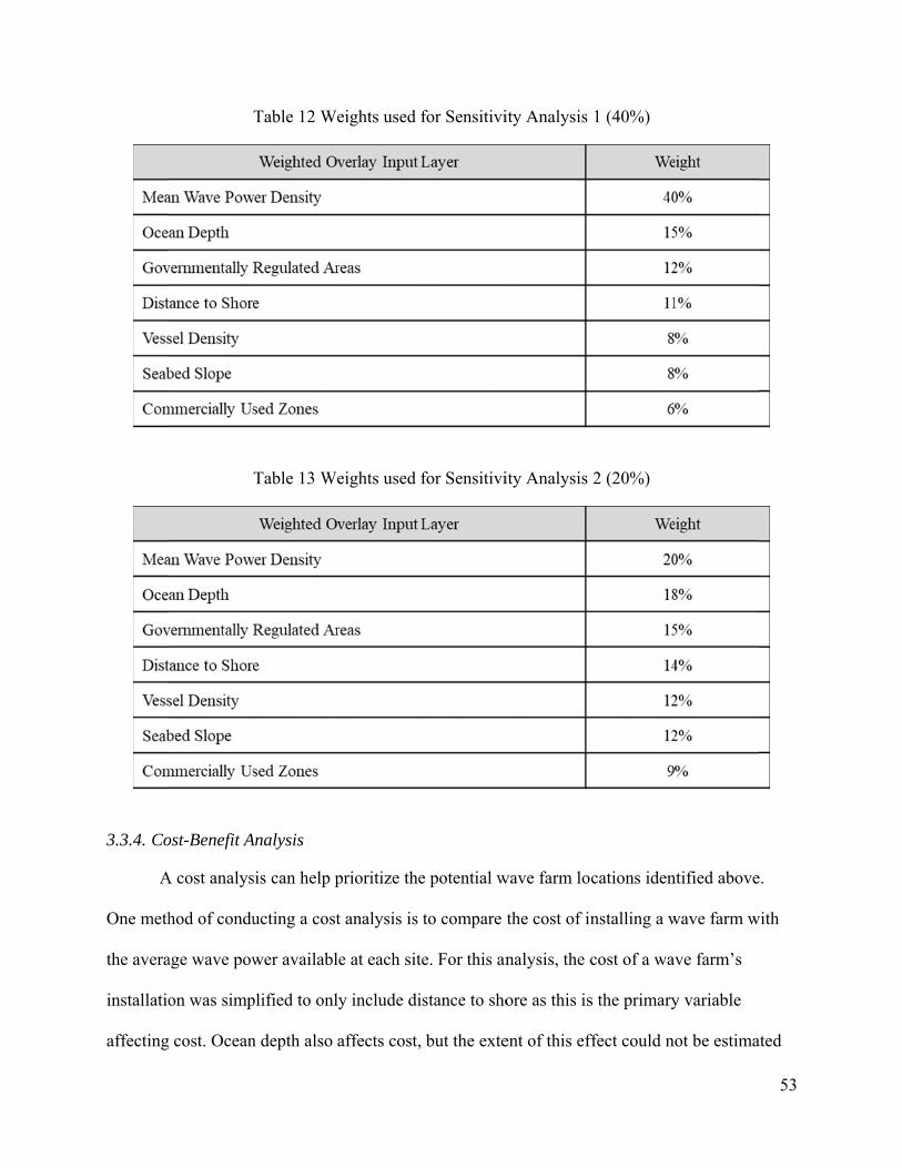
3.3.4. Co
A
One meth
the avera
installatio
affecting
ost-Benefit A
A cost analys
hod of condu
age wave pow
on was simp
g cost. Ocean
Table 12 We
Table 13 We
Analysis
sis can help p
ucting a cost
wer availabl
plified to onl
n depth also
eights used f
eights used f
prioritize the
t analysis is
le at each site
ly include di
affects cost,
for Sensitivi
for Sensitivi
e potential w
to compare
e. For this an
stance to sho
but the exte
ity Analysis
ity Analysis
wave farm lo
the cost of in
nalysis, the c
ore as this is
ent of this ef
1 (40%)
2 (20%)
cations iden
nstalling a w
cost of a wav
s the primary
ffect could no
ntified above
wave farm w
ve farm’s
y variable
ot be estima
53
e.
with
ated

54
so it was left out of this cost analysis. Other values are constants, including cost per WEC device,
cost per kilometer of submarine cable, and the number of WEC devices per site. Since constants
apply to every site equally they do not affect the results of the cost analysis and can be omitted
from this calculation. The simplified fraction between cost and wave power is therefore used as
the cost analysis score:
Cost analysis score = D / P
where D is the distance from site to nearest power station in kilometers and P is the average
wave power per meter of wave crest. For the full cost analysis formula from which this was
simplified, refer to Appendix D.
This cost analysis requires a few assumptions to be met: The wave farm will be
connecting into an existing substation, each WEC device has the same installation cost, and the
full length of the cable to shore will be installed despite preexisting submarine cables.
Furthermore, the number of WEC devices per site is assumed to be a constant and each potential
wave farm site will be large enough to accommodate over 100 PowerBuoys™.

55
Chapter 4 Results and Discussion
The results of the weighted overlay are reported and discussed in three parts in this
chapter. First, a map created from the primary output raster shows the breakdown of final
suitability for wave farms. Second, the sensitivity analyses compared the primary results with the
alternates. Bar graphs depict the percent breakdown per suitability score for each of the three
outputs to compare the variance resulting from a 10% shift in the weight of Wave Power Density
in the weighted overlay. Third, a simple cost-benefit analysis compares the mean wave power of
individual potential wave farm locations along with the distance of each location to the nearest
onshore power station.
4.1. Weighted Overlay Results
The output raster layer from the weighted overlay was broken down into five categories
of suitability, with an increasing score of suitability from Category 1 (least suitable) to Category
5 (most suitable). Category 0 was also included representing restricted areas. A map was
produced for visualization purposes which depicts the layout of these values (Figure 17).
Upon the initial inspection of Figure 12, one might notice that Category 1 is completely
absent from these results. This was due to the fact of relatively few features given this score
which might have been overpowered by multiple layers of higher suitability scores. Category 2 is
the least prominent of the remaining categories with only 200 raster cells grouped together near
the Los Angeles County / Orange County border, nearly indiscernible at the scale used. Next,
Category 3 cells make up several large regions near the center of the study area. Lastly, the
restricted Category 0 falls mainly along the coastline of the mainland as well as each of the
Channel Islands. These first four categories are considered undesirable, if not completely
restricted, for this study.

T
makes up
of these c
as the neu
and Cate
Category
grouping
high imp
within th
are no Ca
The more suit
p nearly 75%
cells, in the m
utral class, w
gory 5 is alo
y 5 are mostl
gs spread out
portance com
he area where
ategory 5 ce
table areas f
% of the cells
map as well
whereas thos
one in consid
ly grouped to
t beyond the
mpared to the
e Wave Pow
lls that fall w
Figure 17
fall within th
s in this raste
as the histog
se scored bel
deration for p
ogether to th
Channel Isl
e other variab
wer Density w
within areas
7 The primar
he 4th and 5th
er layer (Fig
gram, sugge
low 4 (Categ
potentially s
he northwest
lands. Becau
bles, the maj
was also sco
where wave
ry wave farm
h suitability c
gure 18). The
ests that Cate
gory 0 to Ca
suitable wav
t of the study
use wave pow
jority of Cat
ored 5. It is w
e power was
m suitability
categories. C
e abundance
egory 4 shou
ategory 3) are
e farm locat
y area, with s
wer was give
tegory 5 rast
worthwhile to
scored belo
result
Category 4 al
and distribu
uld be consid
e undesirabl
tions. The ce
several smal
en a relative
ter cells fall
o note that th
w 4.
56
lone
ution
dered
le
ells in
ller
ely
here

57
There are areas along the shore that are noticeably lacking any values in the results of the
weighted overlay. These cells are withheld from the weighted overlay and are not relevant to any
statistical analysis. Prominent examples include San Diego Bay, Mission Bay, and San Pedro
Bay (Figure 16). There is also a small strip of missing cells along the coast and surrounding each
island. These missing cells are caused by a lack of original data in the wave energy model and
were therefore assigned no values. Without suitability scores, these areas are omitted from
consideration of wave farm suitability.
Besides above mentioned characteristics in category breakdown (Category 4 and
Category 0, Figure 18 also shows that no cells fall into Category 1 and only 0.003% of the cells
fall into Category 2, essentially 0% as shown in this graph. With these first three categories
excluded, the data appears more normally distributed.
Figure 18 Category breakdown for wave farm suitability by area percentage
Area Percentage (%)10.710.00313.3972.14
3.75
Category543210
Are
a Pe
rcen
tage
(%
)
70
65
60
55
50
45
40
35
30
25
20
15
10
5
0

58
4.2. Sensitivity Analysis Results
Two additional weighted overlays were run, each using a different weighting scheme
primarily to measure the sensitivity of the weight assigned to the wave power input. The results
of these weighted overlays were compared to the results of the primary weighted overlay. The
particular interest was any differences in the percent breakdown of cells between each category
as well as the changes in the spatial distribution of these cells.
4.2.1. Breakdown of Suitability Categories
The first of these weighted overlays (Sensitivity Analysis test 1, or SA1) raised the
weight of wave power density from 30% to 40%. The result was a drastic shift between
Categories 3 and Category 4 (Figure 19). The area percentage of Category 3 rose 18% and that of
Category 4 dropped 18.35%. The other categories combined made up less than a 1% change,
with Category 5 rising only 0.35% and Category 2 rising about 0.017%. There was no change in
the absence of Category 1 cells. Since Category 0 is made up of restricted cells omitted from the
weighted overlay process then the percentage of cells in this category should always remain
constant. In summary, increasing the weight of wave power density decreased the overall
suitability of the results. However, the bulk of this change occurred between two categories of
lesser importance than Category 5, which saw only a marginal increase.

Figure 1
F
power de
shifts in t
7.6%. Th
The rema
with an in
and Cate
trend tow
in Catego
9 Sensitivity
or the secon
ensity was re
the weights,
his decrease
ainder of the
nsignificant
gory 0 as ex
wards a highe
ory 5.
y Analysis 1:
nd weighted
educed from
with the gre
was almost e
e difference w
drop of 0.00
xpected. In co
er rate of sui
Map and su
overlay in se
30% to 20%
eatest change
entirely com
was account
01% in Cate
ontrast to th
itability. Sim
uitability brea
ensitivity an
% (Figure 20
e being in C
mpensated by
ted for by a r
gory 2. Agai
e SA1 weigh
milar to those
akdown with
nalysis test (S
0). These resu
Category 3 as
y an increase
rise in Categ
in, no chang
hted overlay
e results, how
h 40% weigh
SA2), the we
ults showed
s its raster ce
e of 7.26% in
gory 5’s coun
ges were seen
y results, thes
wever, is the
hted wave p
eight of wav
d less extrem
ell count dro
n Category 4
nt by 0.32%
n in Categor
se showed a
e limited gro
59
ower
ve
me
opped
4.
,
ry 1
a
owth

Figure 2
T
minor, bo
overall p
Category
percentag
Similarly
increase
in the pri
considera
4.2.2. Ch
A
wave pow
classified
ArcGIS,
0 Sensitivity
The increase
oth with less
ercentage of
y 5. In the SA
ge from 3.75
y, the increas
from 3.75%
imary weigh
ation given t
hange in Spa
As described
wer had a dr
d as the -1 C
as being one
y Analysis 2:
of area perc
s than 1% inc
f the raster e
A1 weighted
5% to 4.1%,
se of Catego
to 4.07%, a
hted overlay,
the need to e
atial Distribu
above in Se
rastic decrea
ategory in re
e category lo
Map and su
entage in Ca
crease. How
quates to a m
d overlay the
which is a 9
ory 5 cells by
a relative incr
this extra 9
expand the p
ution
ection 4.2.1,
se in overall
ed. These are
ower in the S
uitability brea
ategory 5 in
wever, such a
much larger
e 0.35% over
9.3% relative
y 0.32% in th
rease of 8.5%
.3% and 8.5%
otential site
the SA1 wei
l suitability.
eas were ide
SA1 weighte
akdown with
either of the
a seemingly
change relat
rall change i
e increase of
he SA2 weig
%. With the
% could be u
selection ar
ighted overl
This can be
entified by th
ed overlay th
h 20% weigh
e weighted o
insignificant
tive to the pe
in Category 5
f cells in Cat
ghted overlay
limited area
used as area
rea.
ay using a 4
visualized i
he Differenc
han in the pr
hted wave p
overlays is ve
t change in t
ercent growt
5 increased i
tegory 5.
y resulted in
a of Category
as of seconda
40% weight f
n Figure 21
ce tool, in
rimary weigh
60
ower
ery
the
th of
its
n an
y 5
ary
for
hted

overlay. A
SA1 weig
were unc
Figure
O
categorie
weight in
showed a
density w
category
All +1 Categ
ghted overla
changed in th
e 21 Categor
Opposite yet
es in the SA2
ncrease in wa
an increase i
weight in SA
of suitability
gory areas, i
ay. All other
he SA1 over
ry changes fr
sensitive
similar patte
2 weighted o
ave power d
n category, i
A2, the areas
y.
n green, are
areas not fa
rlay.
rom the prim
e analysis (4
ern changes
overlay with
density, regio
if any chang
beyond the
where the c
alling into eit
mary overlay
40% weight f
can be seen
that of the p
ons southwes
ge at all, in S
islands that
categories inc
ther of these
y (30% weigh
for wave pow
by comparin
primary over
stward beyo
SA1. With th
showed chan
creased from
e classes are
ht for wave
wer)
ng the spatia
rlay (Figure
ond the Chan
he decrease i
nge instead
m the primar
areas which
power) to fi
al distributio
22). With th
nnel Islands
n wave pow
decreased on
61
ry to
h
rst
on of
he
wer
ne

Figure
A
values do
side of th
Chapter 3
between
decrease
also impo
one categ
22 Category
A clear divide
o not intermi
he divide the
3 (Figure 16
suitability sc
of wave pow
ortant to not
gory.
y change from
sensitive
e can be seen
ingle. On on
ey decrease.
6) and these m
cores of 4 an
wer density w
te that neithe
m the prima
e analysis (2
n in both of
ne side of the
A compariso
maps shows
nd 5 in the w
weight prim
er SA1 nor S
ary overlay (3
20% weight f
these maps b
e divide the c
on between t
that this cle
wave power l
marily affects
SA2 resulted
30% weight
for wave pow
between the
category lev
the wave po
ear divide ali
layer. This s
s areas of les
d in an increa
t for wave po
wer)
e classes as th
vel rises whil
ower density
igns with the
shows that th
sser energetic
ase or decrea
ower) to seco
he red and g
le on the oth
map from
e division
he increase o
c waves. It i
ase of more t
62
ond
green
her
or
s
than

4.3. Co
F
suitability
in the nor
cells to th
Site 5 is a
site was c
shore and
distance
by milita
st Analysi
or cost analy
y result in th
rthwest regio
he south of S
an area of C
chosen for sp
d average wa
to the neares
ary use. For t
Figure
is
ysis, five pot
he primary w
on of the stu
San Miguel I
ategory 4 ce
pecific reaso
ave power. D
st onshore po
this analysis
23 Five pot
tential wave
weighted ove
udy area. Site
Island. Site 4
ells adjacent
ons explaine
Distance to s
ower plant w
, the lower s
ential wave
e farm locatio
erlay (Figure
e 2 and Site
4 is an area o
to a restricte
ed further bel
shore was m
while naviga
scores repres
farm locatio
ons were cho
e 23). Site 1
3 are neighb
of Category
ed area near
low, and me
more specifica
ating around
sent more ide
ons chosen fo
osen based o
is an area of
boring group
4 cells near
r San Nicolas
easured for th
ally measure
MPAs and a
eal condition
or cost analy
on their
f Category 5
ps of Catego
Los Angele
s Island. Eac
heir distance
ed by the
areas restrict
ns.
ysis
63
cells
ry 5
es.
ch
e to
ted

S
area; note
Californi
a potentia
kilometer
meter of
F
S
range of
it is still w
and has a
variables
ite 1 was sel
e that the lar
ia Bight. The
al expansion
rs from the n
wave crest.
Figure 24 Th
ite 2 was sel
wave farm p
within an ac
an average w
s into the cos
lected as it is
rge Category
e proximity o
n zone to acc
nearest powe
Inputting th
he potential w
lected as it is
power in the
cceptable dis
wave power o
st analysis eq
s the closest
y 5 site to the
of Site 1 to t
commodate f
er station an
ese variable
wave farm S
s a large gro
study area.
tance. This s
of 20.3 kilow
quation resu
large group
e west is bey
this large gro
future growt
d has an ave
s into the co
Site 1 locatio
ouping of Ca
It is farther
site is 90 kil
watts per me
lted in a sco
ping of Categ
yond the wes
ouping is be
th of the wav
erage wave p
ost analysis r
on with prim
ategory 5 cel
from shore t
lometers from
eter of wave
ore of 4.43.
gory 5 cells w
stern limits o
eneficial as it
ve farm. Thi
power of 19.
resulted in a
mary weighted
lls falling wi
than would b
m the neares
crest. Inputt
within the st
of the South
t could repre
is site is 30
1 kilowatts p
score of 1.5
d overlay
ithin the high
be desirable,
st power stat
ting these
64
tudy
hern
esent
per
7.
hest
, yet
tion

F
S
potential
selected t
importan
closer to
station w
This site
power of
equation
Figure 25 Th
ite 3 was ch
and in size,
to give decis
nt than proxim
the Los Ang
was calculate
is 120 kilom
f 20.3 kilowa
resulted in a
he potential w
osen as an a
but Site 3 is
sion makers
mity to popu
geles metrop
d for the nea
meters from t
atts per mete
a score of 5.9
wave farm S
alternative to
s farther from
the option in
ulation cente
politan area.
arest station
the nearest p
er of wave cr
91.
Site 2 locatio
o Site 2. They
m the neares
n the event t
ers. In this ca
With this in
to the east o
power station
rest. Inputtin
on with prim
y are nearly
st power stat
that the dista
ase, Site 3 w
n mind, dista
of the Chann
n to the east
ng these vari
mary weighted
identical in
tions. Regard
ance to shore
would be ben
ance to the ne
nel Islands, n
and has an a
iables into th
d overlay
wave power
dless, Site 3
e is less
neficial as it i
earest power
near Los Ang
average wav
he cost analy
65
r
was
is
r
geles.
ve
ysis
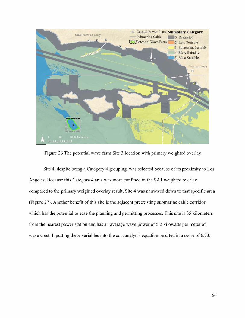
F
S
Angeles.
compared
(Figure 2
which ha
from the
wave cre
Figure 26 Th
ite 4, despite
Because thi
d to the prim
27). Another
as the potenti
nearest pow
est. Inputting
he potential w
e being a Ca
is Category 4
mary weighte
r benefit of th
ial to ease th
wer station an
g these variab
wave farm S
ategory 4 gro
4 area was m
ed overlay re
his site is the
he planning a
nd has an av
bles into the
Site 3 locatio
ouping, was
more confine
esult, Site 4 w
e adjacent pr
and permittin
erage wave p
cost analysi
on with prim
selected bec
ed in the SA
was narrowe
reexisting su
ng processes
power of 5.2
is equation r
mary weighted
cause of its p
1 weighted o
ed down to t
ubmarine cab
s. This site i
2 kilowatts p
resulted in a
d overlay
proximity to
overlay
that specific
ble corridor
s 35 kilomet
per meter of
score of 6.7
66
Los
area
ters
73.

Figure
th
S
cable cor
is consid
is 100 kil
kilowatts
resulted i
27 The poten
e boundary o
ite 5 was sel
rridor. Besid
dered Catego
lometers fro
s per meter o
in a score of
ntial wave fa
of Site 4 wa
lected due to
des, despite b
ry 5 when th
m the neares
of wave crest
f 6.41.
farm Site 4 lo
s defined ba
o its proximi
being a Categ
he weight of
st power stat
t. Inputting t
ocation with
ased on sensi
ity to the ind
gory 4 area i
f wave powe
tion and has
these variabl
h primary we
itivity analys
duction point
in the prima
er was dropp
an average
les into the c
eighted overl
sis 1 result (
t of a preexi
ary weighted
ed to 20% in
wave power
cost analysis
lay (main ma
inset map)
sting subma
d overlay, thi
n SA2. This
r of 15.6
s equation
67
ap);
arine
is site
site

Figure
this loca
T
ideal due
sites. Site
wave pow
fourth du
power po
power re
28 The poten
ation become
The overall c
e to its proxim
e 2 and Site
wer potentia
ue to the high
otential than
lative to the
ntial wave fa
es Category
ost-benefit a
mity to shor
3 were rank
al as Site 1, b
her cost of it
Site 4. Lastl
other sites.
farm Site 5 lo
5 when the w
analysis resu
e as well as
ed second an
but a signific
t being much
ly, Site 4 suf
ocation with
weight of wa
ults can be se
the high ave
nd third, resp
cantly greate
h farther from
ffers in its ra
h primary we
ave power d
een in Table
erage wave p
pectively, as
er distance fr
m shore, but
anking due to
eighted overl
decreases to 2
14. Site 1 w
power comp
s they had si
rom shore. S
t it still had a
o its low ave
lay (main ma
20% (inset m
was the most
ared to other
milar averag
Site 5 is rank
a higher wav
erage wave
68
ap);
map)
r
ge
ked
ve
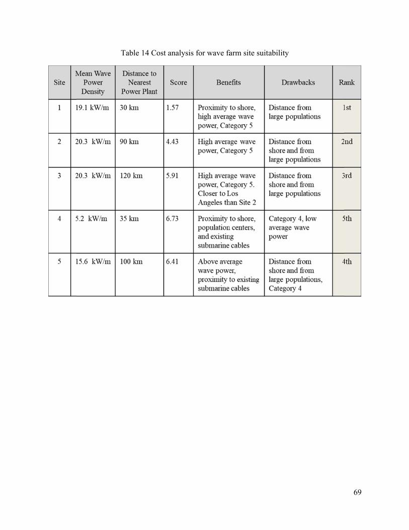
Table 14 CCost analysiss for wave fafarm site suittability
69

70
Chapter 5 Conclusions
The most suitable areas for wave farms within the Southern California Bight (SCB) were
identified based on an extensive set of criteria, including not only wave power but also limiting
factors such as governmentally regulated areas, commercially used zones, vessel density, ocean
depth, seabed slope and distance to the shoreline. This approach assures that the most crucial
elements are considered and weighted according to their importance for the selection of wave
farm sites. Three sites were identified within the SCB during the initial weighted overlay and two
others were selected from the results of the sensitivity analyses. These five potential wave farm
sites were compared against one another and ranked according to their initial cost versus the
estimated average power. A location in the northwestern region of the study area near Point
Conception was selected above the others, primarily due to the higher wave power in that region
along with the site’s proximity to shore. A lack of low scoring limiting factors at this location
earned it a Most Suitable status as Category 5. The only downside of this location is its distance
from major population centers such as Los Angeles and San Diego.
While the Point Conception site and the other four potential wave farm sites scored
highest among the remainder of the study area, the SCB overall is not an ideal location for wave
farms. Due to the average south-southeasterly wave direction of the North Pacific, the SCB is
shielded from much of the ocean’s most powerful waves as pictured in Appendix B. Yet, the
SCB is still moderately suitable only because of the large population that a local wave energy
farm would serve. The limitation in wave power makes a site suitability analysis a critical
process for decision-making in the region.
The International Electrotechnical Commission (IEC) is responsible for creating
International Standards for all electronic or electric related technologies. Their technical

71
specifications for wave resource assessment require a three-part process: preliminary
reconnaissance to identify potential sites, a feasibility assessment of the identified sites, and a
detailed wave farm design plan (Cornett et al. 2014). The process discussed in this thesis should
fall within the first step of this decision making process. Further multi-criteria analysis should be
performed to assess identified locations individually for their quantifiable energy production
potential and economic feasibility. Together, these two analyses will precisely evaluate the actual
suitability and production value of the sites. This process is not limited to the SCB; the
methodology applied in this study can be replicated for any shoreline locations, given the
availability of the necessary data.
5.1. Limitations
There were a few limitations faced within the methods of this study including limitations
of the data, software, and even the status of WEC technology.
One of the major limitations regarding data is the fact that there are so many different
factors to consider for a wave energy farm. Scouring through related research revealed a fair
number of limiting factors yet no source included an array of factors as extensive as those
considered in this study. Even so, there are bound to be at least a few factors which were
unfortunately overlooked. Some factors, on the other hand, were intentionally excluded. For
example, fisheries were not included as the data is not readily available. Commercial fish take, as
an alternative option, was not included in this study because the take tonnage is calculated in a
large grid pattern and would not be useful at the scale of this study. Instead, vessel traffic
somewhat compensated for this gap in the data.
Another limitation with the data was the difficulty in weighing the classes for the
weighted overlay. Research showed that an extensive analytic hierarchy process (AHP)

72
involving a panel of experts given a formal survey showed little promise over a weighted overlay
given equal values to each class. The sensitivity analysis conducted in this study showed that a
moderate change in weighted values could have a large effect on the results. Fortunately, in this
case the changes had a minor effect on the most suitable class (Category 5).
The number of different data sources also presented a problem in this study. Aside from
the difficulty of having to find all required datasets, having multiple sources also made unifying
the data for analysis difficult and time consuming. Differences in coordinate systems, cell sizes,
and extents had to be resolved prior to proceeding. Different sources also held different standards
of accuracy, scale, and completeness that had to be considered along with the issue of dated data.
Some datasets have not been updated in years while others are current. Lastly, others attempting
to replicate this study for a different region might find that all of the data is not globally
available. Wave data, for example, was modeled using a U.S. based array of data buoys meaning
that a different wave modeling technique might be required for projects outside the U.S.
ArcGIS provides many tools and extensions for a broad range of purposes yet wave
modeling is not yet among them. An attempt was made to utilize the Spline with Barriers tool in
ArcGIS as an alternative to a third party wave modeling software, but the results were
inadequate, as shown in Appendix C. This was attempted by using the average wave heights for
each buoy location as the input value points and the land (above sea level) layer to act as
barriers. If the results were promising, the peak wave period values would have been modeled
using spatial interpolation as well. Advanced spatial interpolations available in the Geostatistical
Analysis Tools toolbox in ArcGIS might have generated more suitable results, but these were not
tested.
73
The unsuitable spatial interpolation result of wave power deemed a third party modeling
software to be required, yet this provided its own set of limitations. All promising wave
modeling software was either vastly expensive for a site suitability project like this one, or was
not fully developed into a user-friendly application. Only two free models were found for
consideration: SWAN and MOPS. Both required an advanced level of computing skills (e.g.
FORTRAN) to operate without a graphical user interface (GUI). For this project, it was fortunate
that the creators of the MOPS model were able to assist in running the model themselves and
providing the resulting wave energy rasters.
Choosing the most likely WEC technology that would be selected for use in the SCB
required much research. The state of WEC technology is still a constant flux as more efficient
and less expensive designs are continuously being developed. The most commonly deployed
design is the Pelamis Wave Power attenuator making it the original focus of this study until more
research exposed the fact that all proposed wave farms in the U.S. plan to use the PowerBuoy™
by the company OPT. In another year or two, I expect these designs to evolve or be replaced
completely. With different operating specifications for newer devices, it will likely become
necessary to update the limiting factors—primarily ocean depth—in future projects.
5.2. Improvements and Future Work
This study succeeded where it was meant to. Nevertheless there is always room for
improvement. Apart from the limitations described in the previous section, there are several
additions that might be included in future studies.
One thing that became apparent while conducting research was that wave farms are not
limited to generating energy from waves alone. The terms “hybrid farm” or “dual wind and wave
energy” were used by many different sources in reference to devices which could harness both

74
wind and wave power to generate energy. It was found that the California coast would benefit
greatly from combining these technologies by reducing the idle time during periods of low
resource availability (Stoutenburg, Jenkins, and Jacobson 2010). This might not prove true in the
SCB with its unique wave states as the benefit is minimal in regions with a strong temporal
correlation between resources (Fusco, Nolan, and Ringwood 2010). However, future studies
might consider conducting a site suitability analysis for such a dual-use device by considering
additional limiting factors for wind energy.
Given more time, another addition to this study would be an official survey of experts in
order to conduct a more thorough AHP for the weighting of the site selection factors. The results
would not be expected to vary much, though it would eliminate the impression of guesswork.
Another option would be an extended sensitivity analysis developed to test the effects of altering
the weights of each class rather than just that of wave power.
The cost analysis in this study was effective yet overly simplified. A much more
extensive cost analysis was originally designed to estimate the number of months it would take
for each site to cover the costs of the initial installation of a ten-unit wave farm. Unfortunately,
this cost analysis was exceptionally complex. A more in-depth cost analysis would also require
an engineering feasibility study, for which this project has provided the foundation. In the future,
this in-depth cost analysis can be conducted to provide more accuracy in evaluating the potential
wave farm sites.
One final thought on the improvement of this study would be a more detailed
documentation of the MOP wave model. The instructions provided in this model are limited in
their usefulness. This process thus had to be completed by the scientist team who created the
model. For follow-up studies on wave energy farm site selection, it would be beneficial to gain a

75
better understanding about the modeling software in order to complete the models without this
third party request. A more complete step-by-step tutorial than the brief description provided
would be required.
76
References
Abanades, J., D. Greaves, and G. Iglesias. 2014. “Wave Farm Impact on the Beach Profile: A Case Study.” Coastal Engineering 86 (April). Elsevier: 36–44. doi:10.1016/J.COASTALENG.2014.01.008.
Astariz, S., and G. Iglesias. 2015. “The Economics of Wave Energy: A Review.” Renewable and Sustainable Energy Reviews 45 (May). Pergamon: 397–408. doi:10.1016/j.rser.2015.01.061.
Barclays Official California Code of Regulations. 2017. 14 CCR § 632.
Bento, A. Rute, Eugen Rusu, Paulo Martinho, and C. Guedes Soares. 2014. “Assessment of the Changes Induced by a Wave Energy Farm in the Nearshore Wave Conditions.” Computers and Geosciences 71 (October). Pergamon: 50–61. doi:10.1016/j.cageo.2014.03.006.
Boeker, Egbert, and Rienk Van Grondelle. 2011. Environmental Physics: Sustainable Energy and Climate Change. 3rd ed. West Sussex, UK: John Wiley & Sons, Ltd.
Booij, N, R C Ris, and L H Holthuijsen. 1999. “A Third-Generation Wave Model for Coastal Regions 1. Model Description and Validation.” Journal of Geophysical Research 104 (C4): 7649–66.
Boström, Cecilia. 2011. “Electrical Systems for Wave Energy Conversion.” Digital Comprehensive Summaries of Uppsala Dissertations from the Faculty of Science and Technology 797.
BP. 2017. “BP Statistical Review of World Energy 2017.” doi:http://www.bp.com/content/dam/bp/en/corporate/pdf/energy-economics/statistical-review-2017/bp-statistical-review-of-world-energy-2017-full-report.pdf.
Chang, G., K. Ruehl, C. A. Jones, J. Roberts, and C. Chartrand. 2016. “Numerical Modeling of the Effects of Wave Energy Converter Characteristics on Nearshore Wave Conditions.” Renewable Energy 89 (April). Pergamon: 636–48. doi:10.1016/j.renene.2015.12.048.
Coastal Data Information Program. 2018. “Documentation.” cdip.ucsd.edu/?nav=documents.
Code of Federal Regulations. 2009. 15 CFR § 9.922.
Cornett, Andrew, Mathieu Toupin, Scott Baker, Steffanie Piche, and Ioan Nistor. 2014. “Appraisal of IEC Standards for Wave and Tidal Energy Resource Assessment.” In International Conference on Ocean Energy.
Data Buoy Cooperation Panel. 2018. “Global Data Buoy Observations: A DBCP Implementation Strategy.”
Electric Power Research Institute. 2011. “Mapping and Assessment of the United States Ocean

77
Wave Energy Resource.” Mapping and Assessment of the United States Ocean Wave Energy Resource. doi:1024637.
Emery, K. O. 1960. The Sea Off Southern California, A Modern Habitat Of Petroleum. John Wiley & Sons, Inc.
Foteinis, S., and T. Tsoutsos. 2017. “Strategies to Improve Sustainability and Offset the Initial High Capital Expenditure of Wave Energy Converters (WECs).” Renewable and Sustainable Energy Reviews 70 (April). Pergamon: 775–85. doi:10.1016/j.rser.2016.11.258.
Franzi, Vincenzo, Domenico Curto, Daniele Milone, and Alessia Viola. 2016. “The Desalination Process Driven by Wave Energy: A Challenge for the Future.” Energies 9 (12). doi:10.3390/en9121032.
Fusco, Francesco, Gary Nolan, and John V Ringwood. 2010. “Variability Reduction through Optimal Combination of Wind/wave Resources – An Irish Case Study.” Energy 35 (1). Elsevier Ltd: 314–25. doi:10.1016/j.energy.2009.09.023.
Ghosh, Soumya, Tilottama Chakraborty, Satyabrata Saha, Mrinmoy Majumder, and Manish Pal. 2016. “Development of the Location Suitability Index for Wave Energy Production by ANN and MCDM Techniques.” Renewable and Sustainable Energy Reviews 59 (June). Pergamon: 1017–28. doi:10.1016/j.rser.2015.12.275.
Gorrell, L., B. Raubenheimer, Steve Elgar, and R. T. Guza. 2011. “SWAN Predictions of Waves Observed in Shallow Water Onshore of Complex Bathymetry.” Coastal Engineering 58 (6). Elsevier B.V.: 510–16. doi:10.1016/j.coastaleng.2011.01.013.
Gosnell, Ginger. 2015. “Quadrennial Technology Review: An Assessment of Energy Technologies and Research Opportunities.” Department of Energy.
Gunn, Kester, and Clym Stock-Williams. 2012. “Quantifying the Global Wave Power Resource.” Renewable Energy 44 (August). Pergamon: 296–304. doi:10.1016/j.renene.2012.01.101.
Hricko, Andrea M. 2006. “Ships, Trucks, and Trains: Effects of Goods Movement on Environmental Health.” Environmental Health Perspectives 114 (4): 204–5. doi:ehp0114-a00204 [pii].
Ilyas, Arqam, Syed A.R. Kashif, Muhammad A. Saqib, and Muhammad M. Asad. 2014. “Wave Electrical Energy Systems: Implementation, Challenges and Environmental Issues.” Renewable and Sustainable Energy Reviews 40 (December). Pergamon: 260–68. doi:10.1016/j.rser.2014.07.085.
International Energy Agency. 2016. “Medium-Term Renewable Energy Market Report 2016.” doi:10.1787/9789264188471-en.
International Maritime Organization. 2007. International Convention for the Safety of Life at Sea (SOLAS).

78
IOC/UNESCO. 2011. “A Blueprint for Ocean and Coastal Sustainability. An Inter-Agency Paper towards the Preparation of the UN Conference on Sustainable Development (Rio+20).” Paris.
Khan, N., A. Kalair, N. Abas, and A. Haider. 2017. “Review of Ocean Tidal, Wave and Thermal Energy Technologies.” Renewable and Sustainable Energy Reviews 72 (May). Pergamon: 590–604. doi:10.1016/j.rser.2017.01.079.
Kinsman, Blair. 1965. Wind Waves: Their Generation and Propagation on the Ocean Surface. Englewood Cliffs, N.J.: Prentice-Hall.
Lehmann, Marcus, Farid Karimpour, Clifford A. Goudey, Paul T. Jacobson, and Mohammad Reza Alam. 2017. “Ocean Wave Energy in the United States: Current Status and Future Perspectives.” Renewable and Sustainable Energy Reviews 74 (July). Pergamon: 1300–1313. doi:10.1016/j.rser.2016.11.101.
Long Beach Board of Harbor Commissioners. 2017. “City of Long Beach Adopted Budget for Fiscal Year 2017.” Long Beach.
López, Iraide, Jon Andreu, Salvador Ceballos, Iñigo Martínez De Alegría, and Iñigo Kortabarria. 2013. “Review of Wave Energy Technologies and the Necessary Power-Equipment.” Renewable and Sustainable Energy Reviews 27. Elsevier: 413–34. doi:10.1016/j.rser.2013.07.009.
Los Angeles Board of Harbor Commissioners. 2017. “City of Los Angeles Harbor Department Adopted Annual Budget 2017/2018.” Los Angeles. https://www.hamilton-city.org/ArchiveCenter/ViewFile/Item/365.
Marine and Hydrokinetic Energy Technology Assessment Committee. 2013. An Evaluation of the U.S. Department of Energy’s Marine and Hydrokinetic Resource Assessments. Washington, D.C.: The National Academies Press. doi:10.17226/18278.
Mekhiche, Mike, and Kathleen A Edwards. 2014. “Ocean Power Technologies PowerBuoy: System-Level Design, Development and Validation Methodology.” In 2nd Marine Energy Technology Symposium. Pennington, NJ.
Mørk, Gunnar, Stephen Barstow, Alina Kabuth, and Teresa M. Pontes. 2010. “Assessing the Global Wave Energy Potential.” In 29th International Conference on Ocean, Offshore Mechanics and Arctic Engineering. Shanghai.
National Data Buoy Center. 2018. “Moored Buoy Program.” www.ndbc.noaa.gov/mooredbuoy.shtml.
Nobre, Ana, Miguel Pacheco, Raquel Jorge, M F P Lopes, and L M C Gato. 2009. “Geo-Spatial Multi-Criteria Analysis for Wave Energy Conversion System Deployment.” Renewable Energy 34: 97–111. doi:10.1016/j.renene.2008.03.002.
O’Reilly, W. C., Corey B. Olfe, Julianna Thomas, R. J. Seymour, and R. T. Guza. 2016. “The

79
California Coastal Wave Monitoring and Prediction System.” Coastal Engineering 116. The Authors: 118–32. doi:10.1016/j.coastaleng.2016.06.005.
O’Reilly, W.C., and R.T. Guza. 1993. “A Comparison of Two Spectral Wave Models in the Southern California Bight.” Coastal Engineering 19 (3): 263–82. doi:10.1016/0378-3839(93)90032-4.
Ozkop, E., and I. H. Altas. 2017. “Control, Power and Electrical Components in Wave Energy Conversion Systems: A Review of the Technologies.” Renewable and Sustainable Energy Reviews 67: 106–15. doi:10.1016/j.rser.2016.09.012.
Peter, Jens, Peter Frigaard, Erik Friis-madsen, and Hans Chr. 2006. “Prototype Testing of the Wave Energy Converter Wave Dragon.” Renewable Energy 31: 181–89. doi:10.1016/j.renene.2005.09.005.
Portmann, Helmut H. 2016. “Eyes on the Ocean: NDBC Buoys Supporting Prediction, Forcast and Warning for Natural Hazards.” In Oceans In Action. Stennis Space Center: National Data Buoy Center.
Poullikkas, Andreas. 2014. “Technology Prospects of Wave Power Systems.” Electronic Journal of Energy & Environment, no. April. doi:10.7770/ejee-V2N1-art662.
Reguero, B G, I J Losada, and F J Méndez. 2015. “A Global Wave Power Resource and Its Seasonal , Interannual and Long-Term Variability.” Applied Energy 148. Elsevier Ltd: 366–80. doi:10.1016/j.apenergy.2015.03.114.
Robertson, Bryson, Clayton Hiles, Ewelina Luczko, and Bradley Buckham. 2016. “Quantifying Wave Power and Wave Energy Converter Array Production Potential.” International Journal of Marine Energy 14: 143–60. doi:10.1016/j.ijome.2015.10.001.
Rogers, W. Erick, James M. Kaihatu, Larry Hsu, Robert E. Jensen, James D. Dykes, and K. Todd Holland. 2007. “Forecasting and Hindcasting Waves with the SWAN Model in the Southern California Bight.” Coastal Engineering 54 (1). Elsevier: 1–15. doi:10.1016/J.COASTALENG.2006.06.011.
Rusu, Liliana, and Florin Onea. 2017. “The Performance of Some State-of-the-Art Wave Energy Converters in Locations with the Worldwide Highest Wave Power.” Renewable and Sustainable Energy Reviews 75 (August). Pergamon: 1348–62. doi:10.1016/J.RSER.2016.11.123.
San Diego Board of Port Commissioners. 2017. “San Diego Unified Port District Fiscal Year 16/17 Annual Budget.” San Diego.
Segura, E., R. Morales, J. A. Somolinos, and A. López. 2017. “Techno-Economic Challenges of Tidal Energy Conversion Systems: Current Status and Trends.” Renewable and Sustainable Energy Reviews 77 (September). Pergamon: 536–50. doi:10.1016/j.rser.2017.04.054.
Sørensen, O L E R, Henrik Kofoed-hansen, Morten Rugbjerg, and Lars S Sørensen. 2004. “A
80
Third-Generation Spectral Wave Model Using Unstructured Finite Volume Technique.” In 29th International Conference on Coastal Engineering. Hørsholm, Denmark.
Southwick Associates Inc. 2009. “The Potential Economic and Conservation Impacts of Proposed Marine Recreational Fishing Closures in Southern California.” Alexandria, Virginia.
Stoutenburg, Eric D, Nicholas Jenkins, and Mark Z Jacobson. 2010. “Power Output Variations of Co-Located Offshore Wind Turbines and Wave Energy Converters in California.” Renewable Energy 35 (12). Elsevier Ltd: 2781–91. doi:10.1016/j.renene.2010.04.033.
Thorpe, T. W. 1999. “A Brief Review of Wave Energy.” ETSU-R120: A Report Produced for The UK Department of Trade and Industry. http://lamtengchoy.com/main/uploads/others/1298524568_8914.pdf.
URS. 2009. “Wave Power Feasibility Study Report.” San Francisco.
Vasileiou, Margarita, Eva Loukogeorgaki, and Dimitra G Vagiona. 2017. “GIS-Based Multi-Criteria Decision Analysis for Site Selection of Hybrid O Ff Shore Wind and Wave Energy Systems in Greece.” Renewable and Sustainable Energy Reviews 73 (January). Elsevier Ltd: 745–57. doi:10.1016/j.rser.2017.01.161.
Wang, Liguo, Jan Isberg, and Elisabetta Tedeschi. 2018. “Review of Control Strategies for Wave Energy Conversion Systems and Their Validation: The Wave-to-Wire Approach.” Renewable and Sustainable Energy Reviews 81 (October 2016). Elsevier Ltd: 366–79. doi:10.1016/j.rser.2017.06.074.
Wilson, James H., and Asfaw Beyene. 2007. “California Wave Energy Resource Evaluation.” Journal of Coastal Research 23 (3): 679–90. doi:10.2112/04-0240.1.
Zubiate, L, J L Villate, Y. Torre-Enciso, H C Soerensen, B Holmes, M. Panagiotopoulos, F. Neumann, N. Rousseau, and D. Langston. 2005. “Methodology for Site Selection for Wave Energy Projects.” In 8th European Wave and Tidal Energy Conference (EWTEC08), 1089–95. https://www.researchgate.net/publication/228769826_Methodology_for_site_selection_for_wave_energy_projects.

Appe
Features
endix A. A
in bold are t
A Complet
those consid
e list of poacqui
dered by mul
otential limired sourc
ltiple source
miting factces
es.
tors considdered by a
81
all

App
endix B. G
Wave powe
Global dist
er marked by
(Sour
tribution omean w
y color; annu
rce: Gunn an
of annual wave direc
ual mean wa
nd Stock-Wi
mean wavction
ave direction
illiams 2012
ve power a
n marked by
2)
and annua
y arrows
82
al

Appenndix C. Muap of wavusing the
e power dSpline wit
density inteth Barrier
erpolated rs tool in A
from CDIArcGIS
IP buoy d
83
ata

84
Appendix D. Detailed Return of Investment equation originally intended for the cost-benefit analysis
𝑇𝑈 ∗ 𝑁 𝐷 ∗ 𝑀 𝑂 ∗ 𝐴
𝑃 ∗ 𝑁 ∗ 𝑉 ∗ 𝐻
Where:
T: Number of months until wave farm pays of cost of installation
U: Cost per WEC device = $6 million
N: Number of WECs to be installed = 10
D: Distance from proposed wave farm to shore = Variable
M: Cost of energy transmission cable per meter = $35
O: Average ocean depth of each site = Variable
A: Cost of anchoring cable per meter = Unknown constant
P: Energy produced per hour, dependent on Wave Power = Variable
V: Value of energy per hour at a local rate = 0.178 per kWh
H: Number of hours in a month = 24 × 365 ÷ 12 = 730
85
Appendix E: Definitions
Capacity Factor: The ratio of the actual energy produced by a wave energy converter divided
by the amount of energy that could theoretically be produced from the full-time operation of that
device at its rated capacity (URS 2009).
Clean Energy: Energy sources which minimalize air, water, and land pollutant emissions
(Gosnell 2015). This term is most often related renewable energy sources, but also includes bio-
fuels and nuclear energy as well.
Diffraction and Reflection: Waves interacting with ocean barriers, natural or manmade, will
bend around and behind those objects in what is called diffraction. They also bounce back, or
reflect, off of those barriers. These interactions slow and/or change the direction of the waves
without influence from the seabed (Thorpe 1999).
Peak Wave Period: The time period, in seconds, between waves with the highest spectral
density; as opposed to average wave period which is the average time between each wave
indiscriminate of wave height (Robertson et al. 2016).
Refraction: Waves interact with the seabed as they propagate into coastal shallow waters. This
interaction causes the waves to slow and change direction, bending to conform to the shape of
the underwater terrain (Thorpe 1999).
Renewable Energy: Inexhaustible energy sources are called renewable (Boeker and Van
Grondelle 2011). Examples of renewable energy sources include solar radiation, wind, and water
(rivers and ocean) as these sources are not depleted by human use.

86
Sustainable Energy: Energy sources which fulfill the energy demands of today without
compromising future generation’s ability to meet their energy needs as well (Boeker and Van
Grondelle 2011). Renewable energy and energy efficiency are two main components of
sustainable energy.
Wave Energy: Wave energy is the amount of wave power per a unit of time. It is expressed in
units such as kilowatts per hour (kWh). For example, 1,000 watts per hour for 1 hour is equal to
1 kWh. Note that 1 watt per hour for 1,000 hours is also 1 kWh.
Wave Power: Wave power is the power generated by ocean waves which can be converted into
useable energy. The unit of measurement is Watts (W). In the wave energy example, 1,000 watts
has 1,000x more power and therefore generates the same energy 1,000x faster.
Wave Power Density (aka Wave Energy Flux): Power in waves is concentrated linearly along
the wave crests (Figure 2). This calls for the need of a linear measurement of wave power, watts
per meter of wave crest (Electric Power Research Institute 2011).