copyright by alberto lópez manríquez 2003

Copyright

by

Alberto López Manríquez

2003

The Dissertation Committee for Alberto López Manríquez Certifies that this

is the approved version of the following dissertation:

FINITE ELEMENT MODELING OF THE STABILITY OF

SINGLE WELLBORES AND MULTILATERAL JUNCTIONS

Committee:

Augusto L. Podio, Co-Supervisor

Kamy Sepehrnoori, Co-Supervisor

Martin E. Chenevert

Eric B. Becker

Eric P. Fahrenthold

Carlos Torres-Verdín



by

Alberto López Manríquez, B.S., M.S.

Dissertation

Presented to the Faculty of the Graduate School of

The University of Texas at Austin

in Partial Fulfillment

of the Requirements

for the Degree of

Doctor of Philosophy

The University of Texas at Austin

May 2003

Dedication

I dedicate this work to my adorable children Karla Elizabeth and Carlos Alberto,

hoping it inspires them to pursue great and ambitious goals in their lives.

I am grateful with my wife Adriana for her understanding and support during the

long period of time required to complete this project.

To my parents José Jesús and Consuelo, this work is dedicated with love.

v

Acknowledgements

I want to express my sincere gratitude to Professors Augusto L. Podio and

Kamy Sepehrnoori for their guidance through this research project. I appreciate

their support, patience and tolerance during the development of this work. I

extend my appreciation to the other members of the Dissertation Committee, Dr.

Eric B. Becker, Dr. Eric P. Fahrenthold, Dr. Martin E. Chenevert, and Dr. Carlos

Torres Verdín for their suggestions to complete this work.

I would like to acknowledge the invaluable help and knowledge provided

by all my professors during my studies at the University of Texas at Austin. Their

knowledge added priceless value to my academic career.

My gratitude is also to all the staff in the Petroleum and Geosystems

Engineering and Civil Engineering Departments who with their daily activities

contributed to keeping everything running smoothly.

I would also like to thank my fellow student Baris Guler who helped me to

set up the software and computing system needed to develop this research.

Finally, I express my sincere indebtedness to all those persons in Petroleos

Mexicanos who believed in this project and authorized the financial support

necessary to carry it out successfully.

vi



Publication No._____________

Alberto López Manríquez, Ph.D.

The University of Texas at Austin, 2003

Supervisors: Augusto L. Podio and Kamy Sepehrnoori

This dissertation describes investigation of the stability of single holes and

multilateral junctions in order to optimize their design. The investigation is based

on finite element three-dimensional modeling using the commercial software

ABAQUS. The stability of single holes and multilateral junctions was analyzed at

different orientations in a three-dimensional in-situ stress field. Traditional stress-

displacement analysis in steady-state was coupled with transient phenomena to

compute strain and stress behaviors and changes in pore pressure due to

disturbances created by drilling. This coupled analysis allowed for the inclusion

of time dependent processes and the nonlinear processes that influence the

behavior of the system compounded by rock, fluids contained in the rock, and in-

situ stresses.

vii

The three-dimensional wellbore stability modeling presented here

overcomes the limitations of common assumptions in wellbore stability analysis,

such as linear poroelasticity, homogeneous and isotropic formations, and isotropic

in-situ stress field, because this modeling accounts for the sources of non-linearity

affecting the strain and stress responses of rock.

This study showed that precise knowledge of the in-situ stress field is an

important geomechanical parameter needed to optimize the orientation of a single

wellbore and the orientation of the lateral at the junction in a multilateral scenario

regarding stability. In addition, performing stress-displacement analysis of

multilateral junctions identified critical areas regarding failure in the junction

area. Geometry, placement, and orientation of the junction were analyzed, and the

results provided a real insight to propose strategies to optimize drilling and

completion design of multilateral wells. Comparisons of the predictions of this

numerical approach with experimental data recently published showed that this

numerical approach is reliable for simulating the steady-state phenomena and

some transient phenomena encountered in wellbore stability analysis of both

single holes and multilateral junctions.

viii

Table of Contents

List of Tables ......................................................................................................... xii

List of Figures....................................................................................................... xiii

Chapter 1: Introduction............................................................................................ 1

1.1 Importance of wellbore stability .............................................................. 1

1.2 Multilateral well completion scenarios ................................................... 3

1.3 Organization of this dissertation .............................................................. 5

Chapter 2: An overview of wellbore stability modeling ....................................... 11

2.1 Wellbore stabilty: background .............................................................. 11

2.2 Wellbore stability: literature review....................................................... 12

2.2.1 Single well stability analysis ...................................................... 12

2.2.2 Multilateral well stability analysis ............................................. 18

2.3 Constitutive models ................................................................................ 22

2.3.1 Basic Constitutive Relationships ................................................ 23

2.3.2 Critical State and the Cambridge Model (Cam-Clay) ............... 26

2.4 Failure criterion...................................................................................... 31

2.4.1 Tensile failure criteria ................................................................. 32

2.4.2 Compressive failure criteria ....................................................... 32

2.4.2.1 Is the intermediate stress really important. ..................... 34

2.4.3 Wellbore closure ........................................................................ 37

Chapter 3: Statement of the problem..................................................................... 49

3.1 Elasticity................................................................................................. 49

3.1.1 Differential equations of equilibrium ........................................ 49

3.1.2 Stress-displacement relationships............................................... 50

3.1.3 Stress-strain relationships ........................................................... 51

3.1.4 Displacement formulation of problems in elasticity ................. 52

3.1.5 Stresses around boreholes .......................................................... 54

ix

3.2 Poroelasticity.......................................................................................... 58

3.2.1 Background in poroelasticity ..................................................... 58

3.2.1.1 Terzaghi's principle. ....................................................... 58

3.2.1.2 Biot's theory.................................................................... 59

3.2.2 Stress-strain relationships ........................................................... 61

3.2.3 Displacement formulation of problems in poroelasticity .......... 62

3.2.4 Stresses around boreholes .......................................................... 64

3.3 Boundary conditions ............................................................................... 65

3.4 Switching from a boundary value problem to wellbore stability analysis ................................................................................................ 67

Chapter 4: Numerical approach to the solution of the wellbore stability problem ........................................................................................................ 69

4.1 Computational Modeling ....................................................................... 69

4.1.1 Analytical and Numerical solutions ........................................... 70

4.2 Constitutive models available in ABAQUS ........................................... 72

4.3 Model Definition.................................................................................... 74

4.3.1 Model's geometry for analysis in a single hole .......................... 74

4.3.2 Drilling simulation in a single hole ............................................ 76

4.3.3 Model's geometry for analysis in a multilateral scenario ........... 78

4.3.4 Drilling simulation in a multilateral scenario ............................. 79

4.4 Wellbore stability mathematical model.................................................. 80

4.4.1 General assumptions ................................................................... 80

4.4.2 Governing equations ................................................................... 81

4.4.2.1 Isothermal analysis ......................................................... 83

4.4.2.2 Hydraulic diffusion analysis ........................................... 84

4.4.3 Phenomena in steady state .......................................................... 84

4.4.3.1 Stress-displacement analysis in elasticity....................... 84

4.4.3.2 Stress-displacement analysis in poroelasticity ............... 87

4.4.4 Transient phenomena .................................................................. 89

x

4.4.4.1 Rate of Deformation....................................................... 89

4.4.4.2 Coupled stress-hydraulic diffusion analysis ................... 92

4.5 Solution method used in ABAQUS............................................... 94

4.6 Wellbore inclination and azimuth variation.................................. 96

Chapter 5: Discussion of results ......................................................................... 107

5.1 Stability of a single wellbore ................................................................ 107

5.1.1 Phenomena in steady state ........................................................ 107

5.1.1.1 Effect of assuming different constitutive models: stress-displacement analysis ............................................ 107

5.1.1.2 Effect of wellbore inclination and azimuth variation: stress-displacement analysis ............................................ 112

5.1.1.3 Effect of rock anisotropy: stress-displacement analysis ............................................................................ 119

5.1.2 Transient phenomena ................................................................ 123

5.1.2.1 Rate of deformation...................................................... 123

5.1.2.2 Coupled stress-hydraulic diffusion analysis ................ 125

5.2 Wellbore stability in multilateral scenarios .......................................... 128

5.2.1 Phenomena in steady state ........................................................ 128

5.2.1.1 Elastic stress-displacement analysis ............................. 128

5.2.1.2 Effect of increasing the junction angle ......................... 131

5.2.1.3 Effect of varying the diameter of the lateral hole ......... 133

5.2.1.4 Effect of varying the orientation of the lateral hole ..... 134

5.2.1.5 Effect of changing the depth of placement of the junction............................................................................ 138

5.2.1.6 Independence between holes ........................................ 139

5.2.1.7 Complex multilateral scenarios .................................... 141

Chapter 6: Conclusions and recommendations ................................................... 196

xi

Appendix ABAQUS Input File .......................................................................... 203

Nomenclature ...................................................................................................... 209

References ........................................................................................................... 214

Vita .................................................................................................................... 219

xii

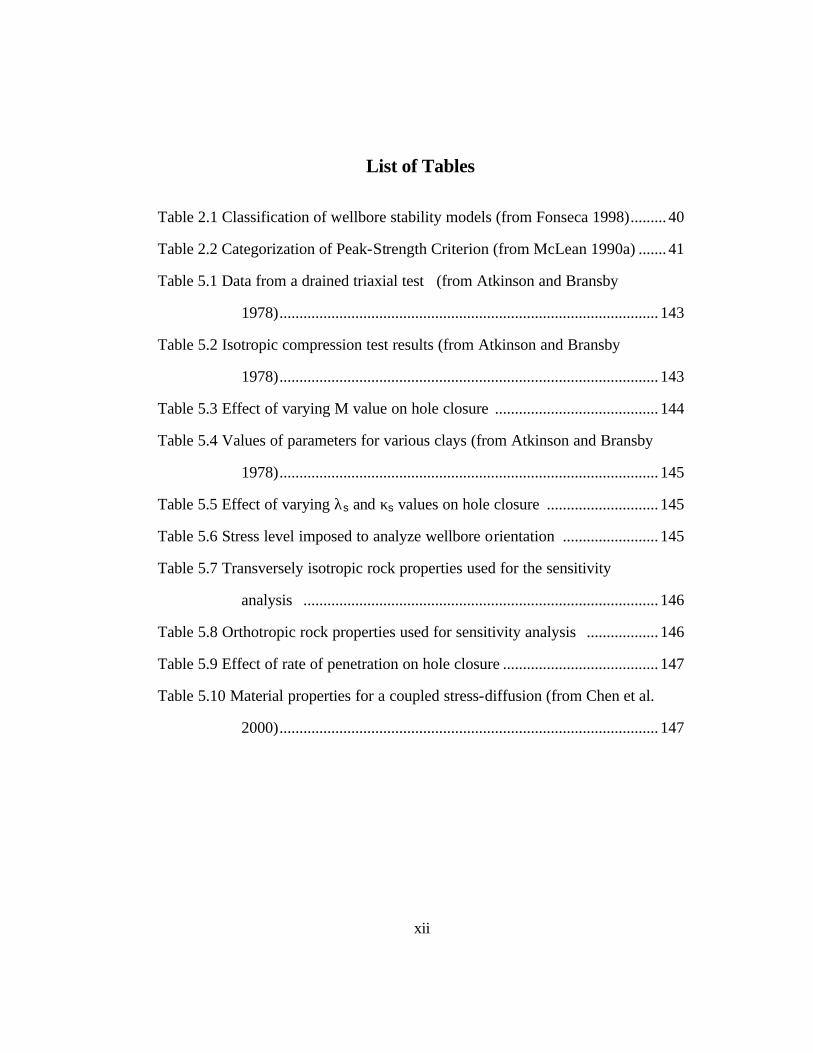
List of Tables

Table 2.1 Classification of wellbore stability models (from Fonseca 1998)......... 40

Table 2.2 Categorization of Peak-Strength Criterion (from McLean 1990a) ....... 41

Table 5.1 Data from a drained triaxial test (from Atkinson and Bransby

1978)............................................................................................... 143

Table 5.2 Isotropic compression test results (from Atkinson and Bransby

1978)............................................................................................... 143

Table 5.3 Effect of varying M value on hole closure ......................................... 144

Table 5.4 Values of parameters for various clays (from Atkinson and Bransby

1978)............................................................................................... 145

Table 5.5 Effect of varying λs and κs values on hole closure ............................ 145

Table 5.6 Stress level imposed to analyze wellbore orientation ........................ 145

Table 5.7 Transversely isotropic rock properties used for the sensitivity

analysis ......................................................................................... 146

Table 5.8 Orthotropic rock properties used for sensitivity analysis .................. 146

Table 5.9 Effect of rate of penetration on hole closure ....................................... 147

Table 5.10 Material properties for a coupled stress-diffusion (from Chen et al.

2000)............................................................................................... 147

xiii

List of Figures

Figure 1.1 Completion levels 1 and 2 according to the Technical

Advancement of Multilateral, TAML................................................ 7

Figure 1.2 Completion levels 3 and 4 according to the Technical

Advancement of Multilateral, TAML................................................ 8

Figure 1.3 Completion level 5 according to the Technical Advancement of

Multilateral, TAML............................................................................ 9

Figure 1.4 Completion level 6 according to the Technical Advancement of

Multilateral, TAML.......................................................................... 10

Figure 2.1 Geometries at the multilateral junction (from Aadnoy and Edland

1999)................................................................................................. 41

Figure 2.2 Definition of independence distance (from Aadnoy and Edland

1999)................................................................................................. 42

Figure 2.3 Comparison between stresses for elastic and plastic solution (from

Charlez 1997a).................................................................................. 42

Figure 2.4 Elastic, hardening, and perfectly plastic behaviors .............................. 43

Figure 2.5 Yield surface (from Atkinson and Bransby 1978)............................... 43

Figure 2.6 Physical phases in plastic collapse (from Charlez 1997a) ................... 44

Figure 2.7 Elastic wall in the three-dimensional p’:q’:v space (from Atkinson

and Bransby 1978)............................................................................ 44

Figure 2.8 Elastic wall and the corresponding yield curve (from Atkinson and

Bransby 1978) .................................................................................. 45

xiv

Figure 2.9 Behavior during isotropic compression and unloading. Hardening

law (from Atkinson and Bransby 1978) .......................……………46

Figure 2.10 Strain increments during yield. Flow rule (from Atkinson and

Bransby 1978) .................................................................................. 46

Figure 2.11 A yield curve as predicted from the Cambridge model (from

Atkinson and Bransby 1978)............................................................ 47

Figure 2.12 Correlation λs – κs (from Charlez 1997a).......................................... 47

Figure 2.13 Common yield surfaces (from McLean 1990b) ................................. 48

Figure 4.1 Pure compression behavior of clay (form ABAQUS/Standard

User's manual, Version 6.1, 2000) ................................................... 99

Figure 4.2. Model mesh for a single hole one step ............................................. 100

Figure 4.3 Effect of mesh refinement in the radial direction on the accuracy of

radial stress calculations ............................................................... 101

Figure 4.4 Effect of mesh refinement in the tangential direction on the

accuracy of radial stress calculations ............................................ 101

Figure 4.5 Effect of mesh refinement in the tangential direction on the

accuracy of tangential stress calculations ..................................... 102

Figure 4.6 Improved accuracy obtained of radial stress calculations in the

nearest region to the wellbore when using “unequally spaced

elements” ....................................................................................... 102

Figure 4.7 Multi- layer model for multi-step drilling ........................................ 103

Figure 4.8 Mutilateral mesh scenario (open view) ............................................ 104

Figure 4.9 Mutilateral mesh scenario (close view) ........................................... 105

xv

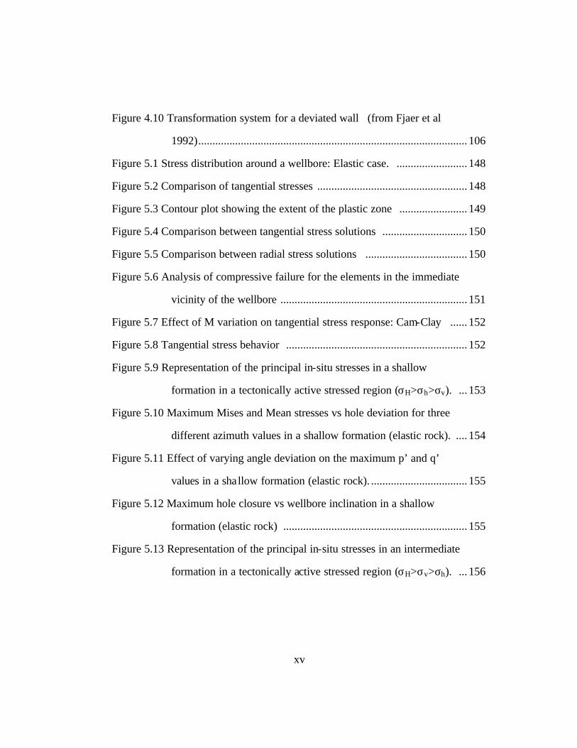
Figure 4.10 Transformation system for a deviated wall (from Fjaer et al

1992)............................................................................................... 106

Figure 5.1 Stress distribution around a wellbore: Elastic case. ......................... 148

Figure 5.2 Comparison of tangential stresses ..................................................... 148

Figure 5.3 Contour plot showing the extent of the plastic zone ........................ 149

Figure 5.4 Comparison between tangential stress solutions .............................. 150

Figure 5.5 Comparison between radial stress solutions .................................... 150

Figure 5.6 Analysis of compressive failure for the elements in the immediate

vicinity of the wellbore .................................................................. 151

Figure 5.7 Effect of M variation on tangential stress response: Cam-Clay ...... 152

Figure 5.8 Tangential stress behavior ................................................................ 152

Figure 5.9 Representation of the principal in-situ stresses in a shallow

formation in a tectonically active stressed region (σH>σh>σv). ... 153

Figure 5.10 Maximum Mises and Mean stresses vs hole deviation for three

different azimuth values in a shallow formation (elastic rock). .... 154

Figure 5.11 Effect of varying angle deviation on the maximum p’ and q’

values in a shallow formation (elastic rock). .................................. 155

Figure 5.12 Maximum hole closure vs wellbore inclination in a shallow

formation (elastic rock) ................................................................. 155

Figure 5.13 Representation of the principal in-situ stresses in an intermediate

formation in a tectonically active stressed region (σH>σv>σh). ... 156

xvi


different azimuth values in an intermediate formation (elastic

rock)................................................................................................ 157

Figure 5.15 Effect of varying angle deviation on the maximum Mean and

Mises effective stresses in an intermediate formation (elastic

rock).......................................................................................…….158

Figure 5.16 Maximum hole closure vs wellbore inclination in an intermediate

formation (elastic rock). ............................................................... 158

Figure 5.17 Representation of the principal in-situ stresses in a deep formation

in a tectonically active stressed region (σv>σH>σh). .................... 159


different azimuth values in a deep formation (elastic rock). .......... 160

Figure 5.19 Effect of varying angle deviation on the maximum Mean and

Mises effective stresses in a deep formation (elastic rock). ........... 161

Figure 5.20 Maximum hole closure vs wellbore inclination in a deep

formation (elastic rock).. ................................................................ 161

Figure 5.21 Maximum Mises stress vs hole deviation for three different

azimuth values in a deep formation (elastic and elastoplastic

cases).. ............................................................................................ 162

Figure 5.22 Comparison of maximum hole closures between the elastic and

the non-elastic cases for three different azimuths in a deep

formation. ....................................................................................... 163

xvii

Figure 5.23 Effect of varying inclination angle on the maximum Mises and

Mean effective stresses. Deep formation (elastic and elastoplastic

cases). ............................................................................................. 164

Figure 5.24 Maximum Mises stresses vs hole deviation at three different Rt

values in a deep transversely isotropic formation (elastic rock). ... 165

Figure 5.25 Comparison of the maximum p’ and q’ values when varying the

deviation angle. Different Rt . Transversely isotropic formation... 166

Figure 5.26 Maximum hole closure vs wellbore inclination. Different Rt.

Transversely isotropic formation.................................................... 167

Figure 5.27 Maximum Mises stresses vs hole deviation at three different Rp

values in a deep orthotropic formation (elastic rock). .................... 168

Figure 5.28 Maximum hole closure vs wellbore inclination. Different Rp.

Orthotropic formation..................................................................... 169

Figure 5.29 Rate of deformation influence on the uniaxial stress-strain curves

and failure of sandstone (from Cristescu and Hunsche 1998)........ 170

Figure 5.30 Comparison of hole closure between one-step and multi-step

analysis. .......................................................................................... 171

Figure 5.31 Progress of drilling with time showing hole closure behind the

advancing face of the wellbore. ...................................................... 171

Figure 5.32 Comparison between pore pressure distribution around a wellbore

for both solutions: elastic and elastoplastic. ................................... 172

Figure 5.33 Contour plot showing pore pressure distribution around a

wellbore after three hours (t=3). ..................................................... 173

xviii

Figure 5.34 Pore pressure distribution as a function of time and radial distance

from the wellbore wall.................................................................... 174

Figure 5.35 Pore pressure distribution as a function of radial distance from the

wellbore wall for different permeability conditions. ...................... 174

Figure 5.36 Effect of yield stress variation on the response of pore pressure

distribution around a wellbore. ....................................................... 175

Figure 5.37 Effect of fluid compressibility variation on the response of pore

pressure distribution around a wellbore. ........................................ 175

Figure 5.38 Distribution of the radial and tangential stresses at the junction

area ................................................................................................. 176

Figure 5.39 Contour plot showing Mises stress. ................................................. 177

Figure 5.40 Contour plot showing displacement in the x-direction ................... 178

Figure 5.41 Stresses in the p’:q’ plane showing changes in the stress cloud .... 179

Figure 5.42 3-D representation showing the three regions A, B, and C

identified at the junction area ......................................................... 180

Figure 5.43 Effect of variation of the junction angle on the stress cloud ............ 181

Figure 5.44 Effect of variation of the diameter of the lateral well on the stress

cloud.. ............................................................................................. 182

Figure 5.45 Contour plot of displacements when the lateral is oriented with an

azimuth (a=90o). ............................................................................. 183

Figure 5.46 Contour plot of Mises stresses when the lateral is oriented with an

azimuth (a=90o) .........…………………………………………….184

xix

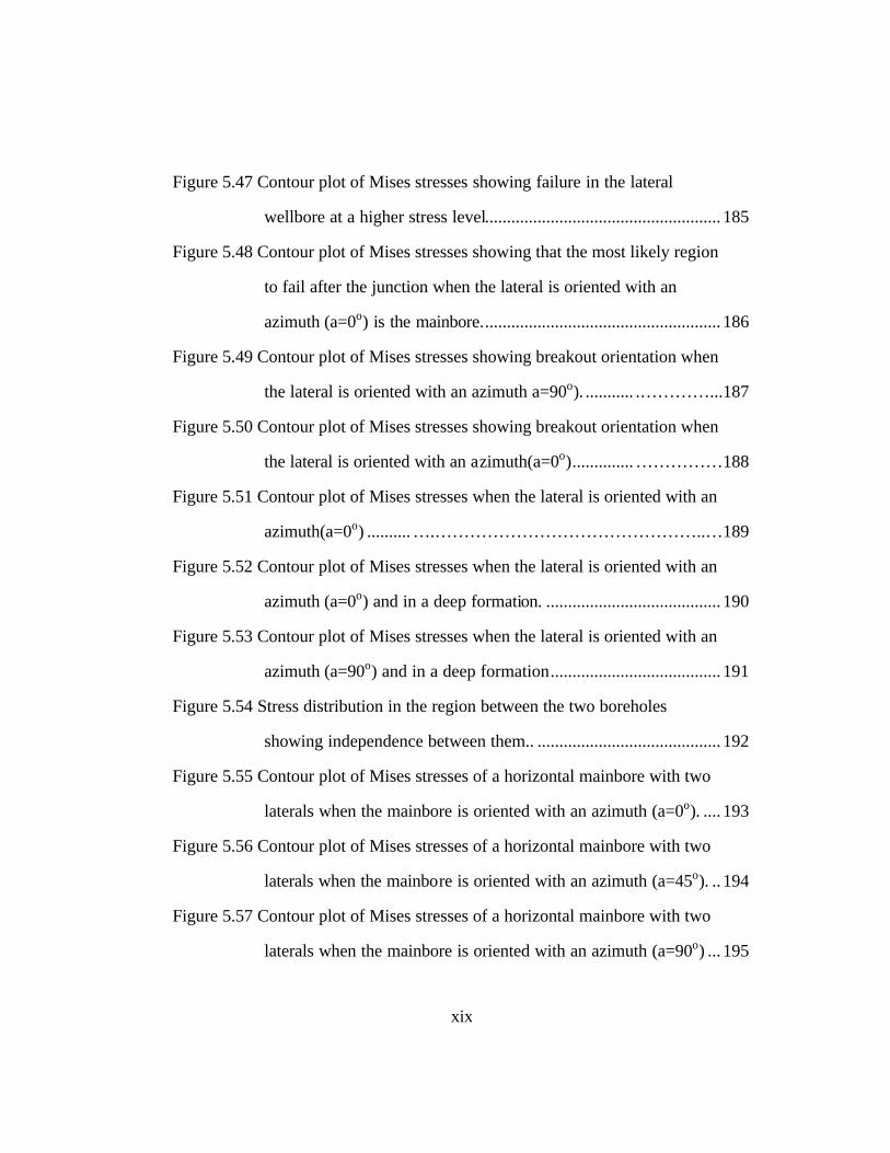
Figure 5.47 Contour plot of Mises stresses showing failure in the lateral

wellbore at a higher stress level...................................................... 185

Figure 5.48 Contour plot of Mises stresses showing that the most likely region

to fail after the junction when the lateral is oriented with an

azimuth (a=0o) is the mainbore....................................................... 186

Figure 5.49 Contour plot of Mises stresses showing breakout orientation when

the lateral is oriented with an azimuth a=90o). ........... .…………...187

Figure 5.50 Contour plot of Mises stresses showing breakout orientation when

the lateral is oriented with an azimuth(a=0o)..............……………188


azimuth(a=0o) ..........….………………………………………..…189


azimuth (a=0o) and in a deep formation. ........................................ 190


azimuth (a=90o) and in a deep formation....................................... 191

Figure 5.54 Stress distribution in the region between the two boreholes

showing independence between them.. .......................................... 192

Figure 5.55 Contour plot of Mises stresses of a horizontal mainbore with two

laterals when the mainbore is oriented with an azimuth (a=0o). .... 193


laterals when the mainbore is oriented with an azimuth (a=45o). .. 194


laterals when the mainbore is oriented with an azimuth (a=90o) ... 195

1

Chapter 1: Introduction

This chapter has the aim to present a general overview of the importance

of wellbore stability in drilling. Initially, brief comments are presented about

general aspects of this topic, followed by a general overview of the scenarios

encountered in multilateral technology and some remarks about the organization

and the structure of the dissertation.

1.1 IMPORTANCE OF WELLBORE STABILITY

Wellbore stability analysis has been the subject of study and discussion for

a long time. The integrity of the wellbore plays a important role in many well

operations during drilling, completion, and production. Problems involving

wellbore stability occur principally through changes in the original stress state due

to removal of rock, interactions between rock and drilling or completion fluids,

temperature changes, or changes of differential pressures as draw down occurs.

For the particular drilling case, support provided originally by the rock is replaced

by hydraulic drilling fluid pressure; this creates perturbation and redistribution of

stresses around the wellbore that can lead to mechanical instabilities. These

instabilities can cause lost circulation or hole closure in the case of tensile or

compressive failure respectively. In severe situations, hole closure can cause stuck

pipe and loss of the wellbore. These events lead to an increase of drilling costs.

The causes of instability have been classified into either mechanical or

chemical effects. A significant amount of research has been focused on these two

2

aspects of instability; the last one mainly oriented to instability in shales.

Although there exists a significant amount of articles related to wellbore stability,

most of them address the study of stability in the vicinity of the wellbore for a

single hole. When two holes interact, the interference that a lateral hole causes on

the stresses around the mainbore is particularly interesting. However, information

about research conducted in a multilateral scenario where two holes interact is

limited. Therefore, the review of literature presented focuses on the status of a

specific area of multilateral wells: the stability of the junction between the

mainbore and the lateral hole.

During the last years, complex well architecture has been implemented as

a new technique to increase well productivity, such as drilling secondary branches

from an existing well. The evolution of multilateral technology has created a wide

range of completion scenarios. Hogg (1997) recognizes that although these new

scenarios have brought new expectations in reservoir management, they have also

created a new set of obstacles, concerns, and risks. To develop a better

understanding of multilateral applications, capabilities, and required equipment,

an oil industry forum on the Technical Advancement of Multilateral (TAML) was

created, and a multilateral classification scheme was developed. Vullings and

Dech (1999) give a complete description of the main characteristics of this

multilateral classification scheme.

3

1.2 MULTILATERAL WELL COMPLETION SCENARIOS

According to Hogg (1997), several factors must be taken into account

when one considers a multilateral project. First, since the goal of the multilateral

is to enhance hydrocarbon recovery, it is crucial to have a good understanding of

reservoir behavior. Secondly, wellbore stability plays an important role;

geological characteristics of the rock must be considered. In addition, even if the

lateral junction is initially competent, the completion system should be designed

for the life of the well. A final consideration for multilateral completion design

should be the need for future workovers requiring re-entry into the lateral or

mainbore with the purpose of periodic cleanouts, stimulations, or any other kind

of workover.

It is interesting to note that although drilling plays a very important role in

multilateral activity, the multilateral classification scheme is based on completion

rather than drilling characteristics. TAML categorizes the multilateral completion

process into levels as a function of risk and complexity.

The goal of multilateral completions is to achieve a junction with full

mechanical and hydraulic integrity by increasing the level of complexity.

According to the TAML classification, there are six different levels of multilateral

completion. The simplest system is Level 1, consisting of branches drilled from a

main open hole. Because little or no completion equipment is required, there is no

mechanical support or hydraulic isolation. The advantage of this system is its low

cost and simplicity. However, the lack of casing limits the installation of

completion equipment, and as a consequence, there is no production control.

4

Furthermore, this kind of completion is limited to competent formations able to

provide borehole stability. The next step in complexity is Level 2. At this level,

the mainbore is cased while the lateral bore is openhole or with a simple slotted

liner. The presence of casing in the mainbore helps to reduce the risk of borehole

collapse, but this is only true in the case where the formation is competent in the

junction area. Figure 1.1 illustrates completion levels 1 and 2 according to

TAML.

The next level of completion is Level 3. This scenario requires the

mainbore to be cased and cemented; the lateral well is cased with a liner, but it is

not cemented. The main advantage of this completion is the mechanical support

given by the casings at the junction area. Therefore, the junction is partially

protected from potential collapse. It is important to remark that although

mechanical support is given, there is no hydraulic isolation at the junction. Level

4 is exactly the same as level 3 from a drilling point of view. However, the main

difference is that both holes are cased and cemented. For this reason, it is

considered that the junction is mechanically protected from collapse. However,

there is no complete hydraulic isolation at the junction since the cement may be

unable to support large differential pressure, or it could fail over time as

drawdawn pressure increases. Figure 1.2 illustrates the characteristics of the levels

mentioned above.

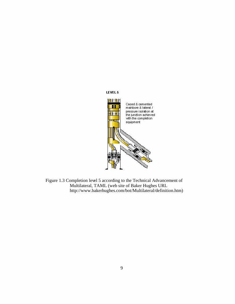
Only levels 5 and 6 provide pressure integrity at the junction, and only

level 6 provides full mechanical and hydraulic integrity. As shown in Figure 1.3,

level 5 completion requires a complex configuration of isolation packers to isolate

5

the junction and provide pressure integrity. In this case, both holes are cased and

cemented, and isolation packers provide three sealing points in the well. Two of

the three are at the junction area in the mainbore; the first one is above, and the

second below. The third one is in the lateral, below the junction. This arrangement

allows isolation of the junction, and as a result, better hydraulic isolation is

achieved where completion equipment works in conjunction with the cement.

Finally, it is important to remark that pressure integrity is achieved with

completion equipment.

The principal characteristic of level 6 completion is that mechanical and

hydraulic integrity at the junction are achieved with the casing using a pre-formed

metal junction, which is installed with the casing itself. Thus, mechanical and

hydraulic integrity are obtained with the casing rather than using completion

equipment. This condition brings some advantages over the lower levels. In

addition to avoiding the risk of handling isolation packer assemblies, it helps to

prevent and to reduce problems related to the quality of the cementing job and the

cement material properties. Figure 1.4 illustrates level 6 completion.

1.3 ORGANIZATION OF THIS DISSERTATION

This introductory Chapter 1 deals with brief comments about the

importance of wellbore stability, mainly in drilling. A general overview about

multilateral well completion scenarios is described. Chapter 2 serves two

purposes. First, it summarizes different approximations to the solution of the

problem of wellbore instability and reviews single and multilateral well stability

6

analyses. With this, the reader has the opportunity to compare what is the state-of-

the-art in each area. Secondly, it points out the importance of choosing an

appropriate constitutive model and an adequate failure criterion to reproduce rock

mechanical behavior and rock failure. Chapter 3 presents the general theory of

material mechanical behavior. It is an overview of the basic formulation of the

general problem in elasticity. For the case of rock analysis, material porosity is

introduced in these theories. Once the formulation of the general problem is

stated, then we switch from the boundary value problem to the wellbore stability

analysis problem.

Chapter 4 aims to support the decision of choosing a commercial finite

element program to conduct this research. It presents the general considerations

for constructing the models using the commercial package. Chapter 5 presents the

analysis of the results obtained by simulation of particular cases. Finally, Chapter

6 presents the conclusions and recommendations for future work.

7

Figure 1.1 Completion levels 1 and 2 according to the Technical Advancement of Multilateral, TAML (web site of Baker Hughes URL http://www.bakerhughes.com/bot/Multilateral/definition.htm)

8

Figure 1.2 Completion levels 3 and 4 according to the Technical Advancement of Multilateral, TAML (web site of Baker Hughes URL http://www.bakerhughes.com/bot/Multilateral/definition.htm)

9

Figure 1.3 Completion level 5 according to the Technical Advancement of Multilateral, TAML (web site of Baker Hughes URL http://www.bakerhughes.com/bot/Multilateral/definition.htm)

10

Figure 1.4 Completion level 6 according to the Technical Advancement of Multilateral, TAML (web site of Baker Hughes URL http://www.bakerhughes.com/bot/Multilateral/definition.htm)

11

Chapter 2: An overview of wellbore stability modeling

This chapter serves two purposes. First, it presents a review of the

literature that is relevant to the solution of the single and multilateral well stability

problems. It provides the opportunity to compare what has been done in each

area. Second, it reviews the importance of choosing an appropriate constitutive

model as well as an adequate failure criterion to analyze wellbore stability

problems.

2.1 WELLBORE STABILITY: BACKGROUND

Simulation of wellbore stability has the purpose of predicting the

redistribution of stresses around the wellbore as result of drilling, completion, or

production operations. The most important elements needed to simulate

geomechanical problems are the rock’s constitutive behavior model and an

appropriate failure criterion. Constitutive behavior models used to forecast

wellbore stability range from those using the theory of elasticity to more complex

models which take into account the theories of elasticity and plasticity, porosity of

the materials, temperature, and time dependent effects. Comparison of the stresses

obtained by using some of these constitutive models with an adequate rock failure

criterion determines whether the rock around the borehole is likely to fail or not.

Fonseca (1998) and McLean and Addis (1990a) include in their works a

classification of wellbore stability models. Table 2.1 shows some special features

that characterize those models for specific purposes.

12

2.2 WELLBORE STABILITY: LITERATURE REVIEW

2.2.1 Single well stability analysis

An attempt to analytically formulate the wellbore stability problem was

done by Bradley (1979a). He used Kirsch’s equations combined with the solution

proposed by Fairhurst in 1968 to develop analytical expressions of stress

distribution around inclined boreholes using the linear elastic theory. Charlez

(1991) explains that Kirsch’s equations were formulated to calculate stresses in an

infinite plate subjected to an initial state of stress. Kirsch’s solution states that the

presence of a circular hole at the center of the plate produces a disturbance within

the solid plate that modifies the initial stress condition. Because Kirsch’s

equations were derived from the assumption that rock was isotropic and

homogeneous, Bradley’s equations keep this condition. Plane strain condition is

also assumed, indicating that the strain component parallel to the wellbore axis is

negligible compared to the radial and tangential strain components. In addition,

Bradley assumed there was no interaction between drilling mud and in-situ

formation fluid.

Bratli et al. (1983) initially investigated the sand problem, which occurs

during production in poorly consolidated sandstones. They focused on the

mechanisms that destabilize the sand behind perforation openings and extended

this theoretical stress analysis to cylindrical wellbores to study stability. Because

they assumed the existence of poorly consolidated material, failure was

considered to be located in a zone around the wellbore, known as the plastic zone.

13

They analyzed the rock stress behavior in this region where high effective stress

concentration occurs.

Aadnoy and Chenevert (1987) and Aadnoy (1988) use Bradley’s approach

to make a detailed analysis about how borehole inclination can influence borehole

stability. They considered two different compressive failure criteria to analyze

borehole collapse: the von Mises and the Jaeger criteria. The first of these takes

into account the intermediate principal stress while the second neglects this.

Jaeger’s criterion, which is an extension of the Mohr-Coulomb criterion, is useful

for laminated sedimentary rocks because it considers the existence of a plane of

weakness that may affect rock behavior. McLean and Addis (1990b) also use

Bradley’s solution, but they focus their analysis by selecting an appropriate failure

criterion to compute safe-drilling fluid densities. They found that when using a

linear elastic constitutive model, the criteria that do not consider the influence of

the intermediate principal stress are likely to underestimate the strength of the

rock.

Earlier work was conducted by considering rock as homogeneous and

isotropic. Aadnoy (1988) and Ong and Roegiers (1993) attempt to provide a better

understanding of the effects of rock properties anisotropies on the stability of a

wellbore. The assumptions they made are that rock behaves as linear elastic

formation, a condition of plane strain prevails, and there is no interaction between

in-situ formation fluids and drilling mud. To fully describe the mechanical

behavior of the rock, the number of elastic constants that Ong and Roegiers

suggest is five: two moduli of elasticity, two Poisson’s ratios and one shear

14

modulus. They concluded that anisotropy strongly influences rock stability,

especially when wellbore inclinations are high or horizontal.

Detournay and Cheng (1988) and Cui et al. (1997) presented ana lytical

solutions for a circular wellbore embedded in a homogeneous and isotropic

formation, which behaves linearly and according to the poroelastic theory. These

solutions are the first attempts to formulate the time-dependent problem

originated from the diffusion process through the porous medium related to the

hydraulic conductivity of the rock. These solutions are restricted to the condition

where the wellbore axis coincides with the direction of the vertical principal

stress. Cui et al. give the analytical solution for a circular wellbore, whose axis is

inclined with respect to the principal stresses, in a linear, poroelastic,

homogeneous, and isotropic formation where the in-situ stresses are anisotropic.

They separate the problem into three parts: poroelastic plane-strain, elastic uni-

axial, and elastic antiplane shear problem. In the first part, they assume that only

in-plane displacements are different from zero. For the second part of the

problem, they claim that the solution is uni-axial and is given by a constant

vertical stress anywhere. For the third part, they explain that the disturbance

caused by the removal of wellbore rock during drilling is introduced to the

analytical problem by a sudden change of shear stress at the wellbore wall.

Finally, they find the final solution by superposition. For wellbore stability

analysis purposes, Drucker-Prager is used as failure criterion.

Another interesting reference is Fonseca (1998). The objective of his work

was to develop a chemical poroelastic model applicable to shales. He considered

15

the poroelastic solution proposed by Detournay and Cheng (1998) to conduct his

research. To investigate the chemical aspect of the instability problem, he took a

microscopic approach of the forces acting in a clay-fluid system, which is based

on the Double-Layer Verwey and Overbeek (DLVO) theory and a macroscopic

approach that evaluates the influence of osmotic potential between shale and

fluid. He found that for a water based mud-shale one-dimensional system, the

total flow of fluid into or out of the shale is driven by two mechanisms: hydraulic

pressure and chemical potential. He reported that the chemical potential can be

introduced into a wellbore stability model as a pore pressure alteration, and it is

controlled by the ratio between the water activity of the shale and the water

activity of the drilling fluid. He concluded that by controlling the water activity of

the mud it is possible to produce a chemical potential that counterbalance the

hydraulic pressure so that the shale behaves as an impermeable formation. A

particular case where a mud with a water activity lower than the water activity of

the shale will induce flow of water out of the shale. This condition is beneficial

for the stability of the wellbore.

Abousle iman et al. (1999) developed software, called Pore-3D, to predict

stability problems during drilling. They claimed that traditional analytical

solutions for wellbore stability, which are based on Bradley’s (1979a) work, fail

to capture the coupled-time dependent phenomenon of stress variation around the

wellbore. They stated that only the analytical solution recently developed by Cui

et al. (1997) considers the coupled-time dependent phenomenon of stress

variation, stating:

16

”The solutions of theories of poroelasticity, porochemoelasticity, porothermoelasticity, and poroviscoelasticity as well as their elastic, chemoelastic, thermoelastic, and viscoelastic counterparts are included in PORE-3D”.

Assumptions involved in this software are that rock formation behaves

linearly when its stress-strain response is analyzed. Moreover, rock formation is

considered homogeneous and isotropic of infinite extent following the

poroelasticity theory. Their development is based on the Cui et al. (1997)

poroelastic solution.

Based on the solution proposed by Lomba et al. (2000a, 2000b) to find the

solute concentration profile in the formation and the poroelastic solution proposed

by Detournay and Cheng (1988), Yu et al. (2001) developed a three dimensional

model to investigate the stress behavior around a wellbore taking into account

chemical and thermal effects in shale formations. They claimed that existing

models, allowing for chemical effect, only take into account the osmotic pressure

effect but do not consider the effect of diffusion of solutes. They concluded that

due to differences between solute concentrations of the drilling fluid and the pore

fluid, competition between water and solute fluxes occurs, altering pore pressure,

which may lead to instabilities.

In recent years, a new modeling approach of wellbore stability has arisen.

Since finite element theory was successfully implemented in other disciplines,

researchers in geomechanics focused their attention on this theory. Pan and

Hudson (1988) developed a couple of nonlinear axisymmetric finite element

models in 2-D and 3-D to study the behavior of stresses and displacements in the

rock surrounding tunnel excavations. They used an elasto-viscoplastic model

17

proposed by Zienckiewicz and Cormeau (1974) that considers the time-dependent

response of the rock associated with its plastic properties. They directed their

study to find the differences between the results predicted by assuming plane

strain in the 2-D model versus the results obtained by the 3-D model.

Development of the 3-D model gave them the opportunity to compare the results

of classical analysis in 2-D, a one-step tunnel excavation, versus multi-step

analysis in 3-D. Among other conclusions, they found that modeling tunnel

excavations in 2-D underestimates deformation compared with the results of the

3-D analysis. They concluded that this discrepancy obeys the plastic response of

the rock behind the tunnel face, a response that a 2-D model cannot reproduce.

Ewy (1993) also used commercial finite element software to study the

behavior of sedimentary rocks to analyze wellbore stability in directional and

horizontal wells. He assumed rock formation behaves according to the

elastoplastic theory. He developed a model in three dimensions (3-D) by

assuming that a “thin slice” of elements orthogonal to the well axis may represent

the rock behavior. Similar analysis was done by Zervos et al. (1998), who

modeled wellbore stability of weak sedimentary rocks for a wide range of

wellbore orientations and deviations. They found that the risk of hole closure

increases as wellbore inclination increases. Orientation of the wellbore becomes

important only for deviations between 30 and 60 degrees. Also wellbores with

inclinations of up to 15 degrees can be treated as vertical wells while for

inclinations of more than 75 degrees, wellbores can be analyzed as horizontal

wells.

18

Chen et al. (2000) developed two numerical models to investigate the pore

pressure diffusion effect in shales. They compared numerical predictions obtained

using a linear and a nonlinear elastoplastic model against those obtained using

experimental observations done with a thick-walled hollow cylinder of synthetic

shale. The analyses demonstrated that for more accurate predictions of stresses

and deformations around a wellbore embedded in shale, the nonlinear model

should be considered because its results showed good agreement with the results

of the laboratory tests.

2.2.2 Multilateral well stability analysis

There exists a considerable amount of publications related to wellbore

stability in a single hole. However, this situation changes radically with respect to

analyses of stability in multilateral junctions. Aadnoy and Edland (1999)

investigated the effect of wellbore geometry on the stability of multilateral

junctions. They assumed that the geometry around the junction takes different

configurations. Above the junction, the hole geometry is circular, which becomes

oval at the junction. Then it splits into two adjacent boreholes below that point, to

finally separate in two independent circular holes. Figure 2.1 illustrates this

situation. They found a relationship between the tangential stress and a stress

concentration factor (Ks) at the wall of the wellbore as shown in Equation 2.1.

They used elasticity theory to set their model.

The tangential stress σθ for an isotropic stress field is represented as

follows:

19

wsHswHsw PKKPKP )1()( −−=−+= σσσθ (2.1)

where

Ks = stress concentration factor

Pw = borehole pressure

σΗ = Maximum horizontal stress

Their approach rests on the assumption that each geometry corresponds to

a different stress concentration factor. First, for circular holes, Ks is a constant

with a value equal to two, Ks = 2. Second, for oval holes, Ks factor is not unique

as is found with circular holes. Instead, there is a Ks value for each of the axes of

the oval geometry. These Ks values are not constant, and they are a function of

n and m values as Equation 2.2 shows.

),( lnfK s = (2.2)

where

l = the vertical/horizontal hole size ratio for the ellipse

n = empirical geometric parameter

Values n and l are functions directly of the geometry of the oval.

According to Aadnoy and Froitland (1991), for the adjacent boreholes condition,

the Ks factor is defined as a function of the distance between holes and the

borehole radius. They found a dimensionless separation distance between holes

20

where the adjacent boreholes can be treated as two independent circular holes.

This distance is expressed as ξ = d/2rw where d is the distance between borehole

centers and rw is the borehole radius. Figure 2.2 illustrates this situation. They

established that the condition to treat the boreholes as independents is ξ > 3. Τhis

model assumes that the two holes are of the same diameter. However, according

to the multilateral completion scheme presented in the previous chapter, holes

have different diameters. The only exception exists in level 6 completion, where

split holes are of the same diameter. Aadnoy and Edland (1999) considered the

Mohr-Coulomb failure criterion, and they also assumed the medium to be

isotropic and homogeneous. Their main conclusion was that the junction is a

critical region where the stress concentration increases as the hole becomes oval.

They found that the oval and the two adjacent holes configurations create extreme

conditions for fracturing and collapse respectively.

Bayfield et al. (1999) showed a particular case of stability at the junction

considering the completion level 6, which means that the junction is cased, and its

integrity is achieved with the casing itself using a pre-formed metal junction.

They performed finite element analysis using a commercial finite element

software to predict the burst and collapse strengths of the pre-formed junction and

then to evaluate the effects of internal and external pressure on the pre-formed

junction, varying the angle between the mainbore and lateral, and cementing the

junction. Their main conclusions are as follows:

21

• Increasing the junction angle from 2.5 to 5 degrees does not

significantly increase burst and collapse strengths.

• Steel reinforcement of the pre-formed junction can significantly

increase junction strength.

• Cement support to the junction can improve burst strength,

depending on the adequate placement of the cement and the

cement properties.

This work aimed at analyzing the resulting stresses along the tubular, the

pre-formed junction, rather than the stress behavior of the rock itself.

Fuentes et al. (1999) present an analysis based on three-dimensional finite

element model, using commercial software to estimate the stress distribution at

the junction. To set up their particular model, they assumed the formation to be

homogeneous sand without shales with no flow between wellbore and formation.

No chemical effects were considered. Other considerations in the model were that

the axes of the global system coincide with the direction of the principal stresses,

and the lateral well is in the direction parallel to the maximum horizontal stress.

The two previous assumptions simplify the problem since no shear stresses occur

when the axes of the system coincide with the direction of the principal stresses.

They used an elastoplastic constitutive model to predict the mechanical behavior

of a sand formation in Lake Maracaibo, Venezuela. Comparing stresses around

the junction region against a compressive failure criterion, they found that the

22

region between the two holes is where stress concentration increases and failure is

more likely to occur.

2.3 CONSTITUTIVE MODELS

Previously, it was mentioned that one of the most important elements to

predict rock behavior is the constitutive behavior model. Choosing an appropriate

constitutive model to simulate rock behavior deeply affects the accuracy of the

results. In this respect, there is still debate over the applicability of some

constitutive models to particular conditions. For instance, it is commonly thought

that wellbores are presumably stronger than the linear elasticity theory predicts.

McLean and Addis (1990a) pointed out that the results of laboratory tests over a

variety of hollow cylinder rock samples show that failure occurs at pressures up to

8 times the failure pressure predicted by linear elasticity used in conjunction with

a failure criterion that does not consider intermediate stress. In the same way,

Charlez (1997a) remarked the significance of plasticity and hardening effects on

stress behavior around wellbores. He mentioned, by comparing the solution based

on a plastic constitutive model to a purely elastic solution, that a plastic zone

surrounding a wellbore exists, which the purely elastic constitutive model is

unable to predict. Figure 2.3 illustrates the comparison between the plastic and the

elastic solutions. The zero value on the radius axis of this figure corresponds to

the wellbore wall. Slight difference can be seen when comparing the radial stress

of the plastic and the elastic solutions. However, considerable relaxation of the

tangential stress occurs in the region nearest to the wellbore (low radius values).

23

Based on this substantial difference of the tangential stress behaviors between the

elastic and the plastic solutions, Charlez (1997a) concluded that there exists a

plastic zone surrounding the wellbore.

2.3.1 Basic Constitutive Relationships

Although it is beyond the scope of this work to give an explanation for

each one of those constitutive models used to describe rock behavior, it is

necessary to briefly mention the principal characteristics of some of the basic

constitutive relations.

The simplest relationship is elastic, which is the foundation for all aspects

of rock mechanics. This theory is based on the concepts of stress and strain,

which are related according to Hooke’s law:

εσ E= (2.3)

The proportionality constant E between stress σ and strain ε is the elastic

modulus. The other parameter required for this model is Poisson’s ratio, which is

a measure of lateral expansion relative to longitudinal contraction. It is defined as

follows:

x

y

ε

εν −= (2.4)

24

However, rocks have what is called “void space”, which is actually

occupied by fluids. Consequently, elasticity theory for solid materials does not

satisfy this condition, and the poroelasticity concept arises. When we talk about

poroelasticity, immediately we should think about two components: solids and

fluids. Therefore, in addition to the variables involved in elasticity, new variables

related to void space and fluid content appear. Thus, a complete description of

rock behavior under this theory requires more than the two simple parameters

considered in the elasticity theory.

Wang (2000) divides poroelastic constants into six different categories: (1)

compressibility bulk modulus, (2) Poisson’s ratio, (3) storage capacity, (4)

poroelastic expansion coefficient, (5) pore pressure buildup coefficient, and (6)

shear modulus. There are three basic material constants: bulk modulus,

poroelastic expansion coefficient, and storage coefficient. However, in order to

define a complete set, a fourth constant has to be considered. This last constant

should include a property related to shear deformation. For instance, Biot and

Willis (1957) suggested the set {G, 1/K, 1/Ku, S}, where 1/Ku is the

compressibility coefficient obtained in an unjacketed test and S is the storage

coefficient. G is the shear modulus. Detournay and Cheng (1988) selected

{G,α, ν, νu} as the complete set of poroelastic constants, where α is the Biot

constant, and ν and νu are the Poisson’s ratios obtained in jacketed and unjacketed

tests respectively.

What happens when elasticity theory is unable to match rock behavior?

Above the elastic limit, the elasticity theory is unable to predict material behavior.

25

Therefore, an appropriate definition of failure criterion and post-failure behavior

are important. Fjaer et al. (1992) mentions that the immediate option for post-

failure behavior is the plasticity theory, although other options such as the

bifurcation theory are available.

Fjaer et al. (1992), Naylor and Pande (1981), and Atkinson and Bransby

(1978) agree that the main concepts supporting the plasticity theory are yield

criterion, hardening rule, flow rule, and plastic strains. Simple definitions about

each concept are as follows: Yield criterion is the point where irreversible

changes occur in the rock. It separates states of stress, which cause only elastic

strains, from those which cause plastic and elastic strains. The hardening rule

describes how rocks under certain conditions might sustain an increasing load

after the initial failure. Flow rule defines the direction of the vector of the plastic

strain increment, δεp, related to the yield surface. Plastic strains take place when a

sample is forced beyond its elastic limit. Total strain, δε, can be expressed as the

summation of the vectors of elastic (δεe) and plastic (δεp) strain increments:

pe δεδεδε += (2.5)

A typical strain-stress diagram for an elastoplastic material is shown in

Figure 2.4. Three different regions can be identified: elastic, hardening, and

perfectly plastic behaviors. Atkinson and Bransby (1978) explain that yielding,

hardening, and failure may be represented on a diagram with axes pca εσσ :: '' as

it is shown in Figure 2.5, where 'aσ and '

cσ are the axial and compressive

26

effective stresses respectively applied on a sample in a conventional “triaxial”

test. This figure shows a set of yield curves such as GaGc, each curve associated

with a particular plastic strain value εp. All curves together define a particular

yield surface shown in Figure 2.5. The yield surface is limited by the curve YaYc

which corresponds to the yield when εp=0 and by the failure envelope FaFc. The

hardening behavior is represented by the response of curve GaGc to plastic strains,

εp.

It is accepted that clays are the main cause of wellbore instability

problems during drilling. Therefore, it is important to have a constitutive model

equipped to handle clay behavior. The literature review showed that, in general,

wellbore stability analysis is done by considering either elasticity or poroelasticity

theories. However, recent numerical approaches have taken into account the

plastic response of rock. Charlez (1991) and Brignoli and Sartori (1993) point out

the importance of two classical elastoplastic models used in geomechanics that

take into account the role of clays. These are the Cambridge model (Cam-Clay)

and the Laderock model, which are both critical state models.

2.3.2 Critical State and the Cambridge model (Cam-Clay)

Charlez (1991, 1997a) reviews the limits of the Cam-Clay model. He

remarks that there are different phases in the plastic collapse mechanism

associated to rock’s volumetric deformation. He establishes that, for ductile rocks

under increasing loading, three phases are observed: (1) rupture of bonds, (2)

plastic collapse, and (3) consolidation. These regions are illustrated in Figure 2.6.

27

However, not all rocks exhibit these three phases. For instance, for

unconsolidated sands and shales, there is not enough cohesion between the grains.

Hence, only a consolidation phase exists.

It is here where soil mechanics begins playing an important role, and the

Cam-Clay model can be selected to analyze shale behavior. Atkinson and Bransby

(1978) discussed in depth the theory of critical state. Because it is complex, here it

is presented only in a brief description of its principles.

There are important definitions in soils mechanics, such as the Roscoe and

Hvorslev surfaces, representing the state boundary surfaces for normal and

overconsolidated materials respectively. Elastic wall, critical state line, normal

consolidation line, and swelling line are also important elements of soils

mechanics analysis. These elements are represented in the q’:p’:v space, shown in

Figure 2.7, where q’ and p’ are known as stress invariants in terms of the effective

stresses ( )'3

'2

'1 ,, σσσ defined according to Equations 2.6 and 2.7. v is the specific

volume of the sample defined as v=1-e, and e is the void space. For a general

three dimensional state of stress, q’ and p’ become:

( ) ( ) ( )[ ]

( )'''31

'

''''''2

1'

321

21

213

232

221

σσσ

σσσσσσ

++==

−+−+−==

pp

qq

eff

eff

(2.6)

For a triaxial stress state, where the horizontal stresses are equal ( )'3

'2 σσ =

and ( )radialaxial σσσσ == '2

'1 ; , these q’ and p’ values are determined by the

following equations:

28

( )radialaxialeff

radialaxialeff

pp

qq

σσ

τσσ

231

'

2'

+==

=−== (2.7)

Atkinson and Bransby (1978) provide the details on how to merge the

yield criterion, the hardening rule, the flow rule, and plastic strains into the Cam-

Clay model.

First, they introduce the concept of elastic wall to show the wall’s

corresponding yield curve. Figure 2.8(a) illustrates the concept of elastic wall in

the three-dimensional space p’:q’:v, with its corresponding projections to the

p’:q’ and p’:v planes shown in Figures 2.8(b) and 2.8(c). These projections are the

yield curve (L’,M’,N) on the p’:q’ plane and the swelling line (L”,M”,N”) on the

p’:v plane respectively. Atkinson and Bransby (1978) say, “For sample states on

the elastic wall and below the state boundary surface, the strains will be purely

elastic and recoverable”. They also define that plastic strains only occur when the

sample state touch the state boundary surface, shown in Figure 2.7. In this sense,

the state boundary surface plays equal role to the yield surface illustrated in

Figure 2.5 in pure plasticity.

Secondly, the hardening rule is obtained by an isotropic compression and

swelling laboratory test on a sample. Typical results of this kind of test are shown

in Figure 2.9. Isotropic compression is represented along the normal consolidation

line to point B, then swelling to point D, compression to point B then point C, and

finally swelling to point E. It is assumed that the sample behaves elastically

29

everywhere except during the loading from B to C where plastic irrecoverable

volumetric strain occurs. These particular plastic strains give enough information

to calculate the hardening behavior of the rock.

A flow rule representation is given in Figure 2.10. The direction of the

vector plastic strain increment δεp, represented by the (QR) vector, is normal to

the yield curve. The flow rule then relates the gradient ( )pv

ps dd εε / of vector (QR)

with the stress applied to the sample represented by (OQ) vector.

The Cam-Clay model, which is valid for normally consolidated materials,

offers one of the alternatives to relate the components of the elastoplasticity

theory. The flow rule is expressed by Equation 2.8.

''

pq

Mdd

ps

pv −=

εε

(2.8)

where M is defined as the slope of the critical state line, identified in Figure 2.11,

on the p’:q’ plane.

The yield curve associated with this flow rule is calculated by the

following equation:

1''

ln'

'=

+

xpp

Mpq

(2.9)

30

where p’x is the value of p’ at the intersection of the yield curve with the

projection of the critical state line at point X as it is shown in Figure 2.11.

At this particular point, the equation of the Cam-Clay state boundary

surface can be obtained and expressed as follows:

( )'ln'

' pvkk

Mpq sss

ss

λλλ

−−−+Γ−

= (2.10)

where λs and κs coefficients are the slopes for the normal consolidation line and

the swelling line respectively, and Γ is defined as the value of v corresponding to

p’=1.0 kNm2 on the critical state line.

Charlez (1997a) published a correlation between λs and κs useful over a

large range of values, which is shown in Figure 2.12. There exists a direct

relationship between these two coefficients where large λs values correspond to

large κs values.

The state boundary surface intersects the v:p’ plane along the normal

consolidation line where q’=0 (see Figure 2.7), and Equation 2.10 reduces to:

'ln pNv sλ−= (2.11)

where ss kN −+Γ= λ .

31

For the critical state line, the specific volume of the sample v is defined by

'ln pv sλ−Γ= , and the Equation 2.10 simplifies to:

'' Mpq = (2.12)

The constitutive relationships discussed in this section will be used in this

work to predict rock behavior in wellbore stability analysis. Chapter 3 presents

the basic formulation of a general boundary value problem using the elastic and

poroelastic constitutive relationships.

2.4 FAILURE CRITERION

Properly choosing the failure criterion is as important as the correct

selection of the constitutive model. The simplest type of criterion is based on the

assumption that the system remains mechanically stable until a certain stress or

strain failure value is achieved (Charlez 1997b). For instance, in a purely elastic

analysis, the stresses are compared against a peak-strength criterion, normally

defined in terms of principal stresses. However, the view that the failure of the

system depends on a single localized point has been debated and considered

pessimistic. On the other hand, when plastic properties of the rock are taken into

account, rock behavior is characterized by a yield criterion. In this case, plastic

strains develop once the stress state reaches the yield criterion instead of at a

peak-strength point.

32

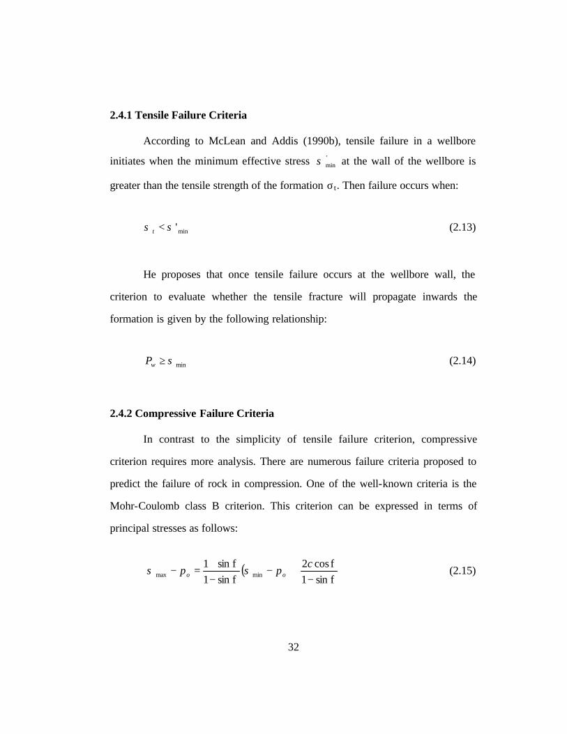
2.4.1 Tensile Failure Criteria

According to McLean and Addis (1990b), tensile failure in a wellbore

initiates when the minimum effective stress 'minσ at the wall of the wellbore is

greater than the tensile strength of the formation σt. Then failure occurs when:

min'σσ <t (2.13)

He proposes that once tensile failure occurs at the wellbore wall, the

criterion to evaluate whether the tensile fracture will propagate inwards the

formation is given by the following relationship:

minσ≥wP (2.14)

2.4.2 Compressive Failure Criteria

In contrast to the simplicity of tensile failure criterion, compressive

criterion requires more analysis. There are numerous failure criteria proposed to

predict the failure of rock in compression. One of the well-known criteria is the

Mohr-Coulomb class B criterion. This criterion can be expressed in terms of

principal stresses as follows:

( )fsin1fcos2

fsin1fsin1

minmax −+−

−+

=−c

pp oo σσ (2.15)

33

where c = cohesion of the sample, po = pore pressure, and f = angle of internal

friction.

On the other hand, the Drucker-Prager (extended Von Mises) category A

criterion is expressed as follows:

( )ooctooct pm −+= σττ (2.16)

where τo and m are Drucker-Prager parameters defined in Equation 2.17.

( ) ( ) ( )

( )minintmax

2maxmin

2minint

2intmax

3131

σσσσ

σσσσσστ

++=

−+−+−=

oct

oct

(2.17)

There are three alternatives in using this criterion for investigating

wellbore stability: the outer, the middle, and the inner Drucker-Prager circles. The

values of τo and m for each alternative are given by Equations (2.18). McLean and

Addis (1990b) discussed the differences in predicting mud weight values as a

result of choosing these different compressive failure criteria. His conclusions are

ambiguous; he says that by using any of the three alternatives given, they may be

successful in one situation, but extremely unrealistic under different conditions.

He presented two different cases of wellbore stability in sandstones.

For the first case, he concluded that, for vertical wells, the Mohr-Coulomb

criterion was in agreement with the inner and middle circle versions of the

Drucker-Prager criterion. As wellbore deviation increases, the two versions of the

34

Drucker-Prager criterion predicted higher mud density requirements than Mohr-

Coulomb. On the other hand, the outer circle version of Druker-Prager was in

agreement with real data values of vertical and horizontal wells.

However, for the second case, when weaker sand with lower cohesion and

friction angle was used, the results between the outer circle version of Drucker-

Prager and the real data field were no longer in agreement. He concluded that

linear failure criteria are applicable to wellbore stability analysis. Only in the

cases of very weak formations with a uniaxial strength less than 1500 psi (10

MPa), a nonlinear criterion may be justified. Figure 2.13(a) shows the projection

of the Mohr-Coulomb criterion and one of the Drucker-Prager circles. Figure

13(b) compares all the Drucker-Prager circles with the Mohr-Coulomb criterion in

the π plane (a plane perpendicular to the line defined when the three principal

stresses are equal ( )minintmax σσσ == .

Outer circle: fsin3fsin22

−=m

fsin3fcos22

−=

coτ

Middle circle: fsin3fsin22

+=m

fsin3fcos22

+=

coτ (2.18)

Inner circle: fsin39

fsin62+

=m fsin39

fcos620

+=

cτ

2.4.2.1 Is the intermediate stress really important?

The importance of whether the intermediate stress (σint) should or should

not be taken into account in the failure criterion for wellbore stability purposes

has been discussed for a long time, and is being debated. Several authors have

35

discussed at length the importance of σint: Mogi (1967), Handin et al. (1967),

McLean and Addis (1990a), Addis and Wu (1993), and numerous others. There

are a variety of reasons for the disagreement related to the significance of the so-

called intermediate stress.

Mogi (1967) established that there are three critical disagreement points

that arise from experimental uncertainties. First, an unknown degree of anisotropy

in rocks, second, inhomogeneity of stress distribution, and third, lack of accuracy

of the failure stress measurements. In this respect, Ong and Roegiers (1993)

agreed with the influence of anisotropy as source of uncertainty. He pointed out

that the usual assumption of rock strength isotropies have been deemed to be

inadequate in describing rock failure under field conditions. To address this

problem, he used a three-dimensional anisotropic failure criterion in conjunction

with the linear elastic theory. The great limitation of this approach is that to fully

describe the mechanical response of rock, the number of elastic constants required

to perform analyses is five: two moduli of elasticity E1 and E2, two Poisson’s

ratios ν1 and ν2, and one shear modulus G, information which most of the time is

unavailable.

Likewise, Handin et al. (1967) established that assumptions such as:

constant temperature, constant strain rate, and mechanical properties of rock

depending only on the state of stress in the material, cause lack of accuracy of

failure criteria. Contrarily, he believed that rock properties are functions at least of

these three factors: state of stress, temperature and strain rate. His main

conclusions were that in the ductile response region, the Von Mises yield

36

condition holds reasonably; in addition, in both the brittle region and the brittle-

ductile transition zone, the shear strength depends on the intermediate stress.

Mogi (1967) agreed with the first of Handin’s conclusions by saying that “In

ductile states failure stresses of rocks are roughly independent of pressure, so that

the Von Mises criterion seems to apply, as for ductile metals.”

McLean and Addis (1990a) separated the different peak-strength failure

criteria in four categories (A, B, C, and D) shown in Table 2.2. According to

McLean, the main problem with many of the criteria which consider the

intermediate stress is that they give great importance to the influence of that

stress. He recognized its importance, but he believed the manner in which Mogi

(1967) incorporated σint into the failure criterion for competent rock as more

reliable. Instead of expressing the stress invariants σoct and τoct in the traditional

way (Equations 2.19), Mogi introduces a weight factor, δ, into the normal

effective stress octσ , which is function of the rock properties (Equation 2.20). He

found that for the four brittle rocks that he tested (Westerly granite, Dunham

dolomite, Darley Dale sandstone, and Solenhofen limestone), the δ value is nearly

the same ( 1.0≅δ ).

( ) ( ) ( )

( )minintmax

2maxmin

2minint

2intmax

3131

σσσσ

σσσσσστ

++=

−+−+−=

oct

oct

(2.19)

where σoct and τoct are octahedral normal and octahedral shear stresses.

37

[ ]minintmax21

σδσσσ ++=oct (2.20)

where σmax, σint, and σmin are the maximum, intermediate, and minimum principal

stresses expressed at the wellbore wall by:

22

max 22 zzz

θθθ τ

σσσσσ +

−+

+=

22

int 22 zzz

θθθ τ

σσσσσ +

−−

+= (2.21)

wP=minσ

where σr, σθ, and σz are the radial, tangential, and axial stresses, and zθτ is the

shear component.

Besides Mohr-Coulomb and Drucker-Prager, there are many others

different compressive failure criteria based on the evaluation of stresses.

However, the importance of the intermediate stress and the consideration that

failure of rocks depends on a single localized point remains in controversy.

Consequently, in recent years, a different class of criterion that evaluates the

maximum wellbore closure allowed has emerged.

2.4.3. Wellbore Closure

Wellbore closure depends on the stress-strain response of the rock and the

stress field, and it can be used as a criterion to identify wellbore instability. Rather

38

than using an ultimate strength limit, wellbore closure is based on the evaluation

of strains until certain strain value is achieved. Ewy (1993) defined this criterion

based on the clearances needed around the drilling tools to allow them to work

properly. The wellbore closure allowed would depend on the size of the tools

being used and the kind of operations being carried out. Therefore, it is not

unique. The review of the literature showed that the accepted value of wellbore

closure allowed is 2% of the wellbore radius. Due to its simplicity and physical

meaning, this is an important parameter in analyzing wellbore stability since

wellbore closure directly affects drilling operations.

The literature review has shown that most of the research in wellbore

stability has focused on two main aspects. These are wellbore instabilities

attributed to mechanical and chemical effects. In addition, most of the research

has been oriented towards the study of stability in the vicinity of a single

wellbore. Significant research has not been conducted in multilateral scenarios to

understand the behavior of rock in the region where two or more wellbores

intersect, region known as the junction. The primary objectives of this research

are as follows: First, to understand rock behavior during drilling of a single

wellbore and then of the junction between the mainbore and the lateral hole, and

second, to propose strategies for design of multilateral wells. Selection and

implementation of an appropriate constitutive model constitutes an important task

of this research to understand the effects of rock anisotropy and stress anisotropy

on wellbore stability. Other aspects such as geometry and placement of the

39

junction and orientation of the lateral wellbore are addressed to evaluate their

effect on the stability of the junction.

40

Table 2.1 Classification of wellbore stability models (from Fonseca 1998).

Reference Model type Special features Bradley (1979) Fuh et al. (1988) Aadnoy and Chenevert (1987) McLean and Addis (1990) Zhou et al. (1996)

Linear elasticity Directional wells

Santarelli (1987) Stress-dependent elasticity

For laboratory analysis. Includes pre-peak yielding

Wang (1992) Mian et al. (1995)

Stress-dependent elasticity

Includes the chemical effect (water content concept)

Paslay and Cheatham (1963)

Linear elasticity Allowancee for fluid flow

Hsiao (1998) Yew and Liu (1992)

Linear poroelasticity Stress at wellbore wall

Mody and Hale (1993) Linear poroelasticity Stress at wellbore wall and chemical effect (osmotic potential concept)

Sherwood (1993, 1994, 1995) Wong and Heidug (1995)

Linear poroelasticity Chemical effect (chemical potential of each species). For laboratory analysis

Detournay and Cheng (1988) Cui (1995)

Linear poroelasticity Simulates the instantaneous drilling effect

Ewy (1991) Mc Lean (1989) Wetergaard (1940)

Elasto-pasticity

Veeken et al. (1989) Elasto-plasticity Incorporate hardening and softening behavior

41

Table 2.2 Categorization of Peak-Strength Criterion. (from McLean 1990a).

Function of σx, σy, & σz Function of σx & σz only

Linear Criterion

Category A e.g. Drucker-Prager

Category B e.g. Mohr-Coulomb

Non-Linear Criterion

Category C e.g. Pariseau

Category D e.g. Hoek-Brown

Single hole Oval Hole

Two Adjacent holes Two Independent holes

Figure 2.1 Geometries at the multilateral junction. (from Aadnoy and Edland 1999)

42

σy

σx σx

d= 2ξrw

σy

Figure 2.2 Definition of independence distance (from Aadnoy and Froitland 1991).

0

2

4

6

8

10

12

14

16

18

20

0 0.1 0.2 0.3

Radius (m)

Str

ess

(MP

a)

Radial stress:Elastic

Tangential stress:Plastic

Tangential stress:Elastic

Radial stress:Plastic

Plastic zone

Figure 2.3 Comparison between stresses for elastic and plastic solution (from Charlez 1997a).

43

σ Perfectly plastic

Hardening

Elastic

ε

Figure 2.4 Elastic, hardening, and perfectly plastic behaviors.

Figure 2.5 Yield surface (from Atkinson and Bransby 1978).

44

Figure 2.6 Physical phases in plastic collapse (from Charlez 1997a).

Figure 2.7 Elastic wall in the three-dimensional p’:q’:v space (from Atkinson and Bransby 1978).

P

1 3 1. Initial material 2. Grains free after rupture of the bonds. 3. Consolidation

Volumetric deformation

2

2 31

45

Figure 2.8 Elastic wall and the corresponding yield curve (from Atkinson and Bransby 1978).

46

Figure 2.9 Behavior during isotropic compression and unloading. Hardening law (from Atkinson and Bransby 1978).

Figure 2.10 Strain increments during yield. Flow rule (from Atkinson and Bransby 1978).

47

Figure 2.11 A yield curve as predicted from the Cambridge model (from Atkinson and Bransby 1978).

0

0.05

0.1

0.15

0.2

0.25

0.3

0 0.2 0.4 0.6 0.8

λs

ks

Figure 2.12 Correlation λs – ks (from Charlez 1997a).

48

Figure 2.13 Common yield surfaces (from McLean 1990b).

49

Chapter 3: Statement of the problem

This chapter presents the basic formulation of a general boundary value

problem in elasticity and poroelasticity. Once the formulation is stated, then we

switch from a boundary value problem to a wellbore stability problem by

imposing a suitable failure criterion.

3.1 ELASTICITY

In practice, generally only the simplest rock properties data are available

for wellbore stability investigation. Because the linear elasticity theory only

requires two parameters: Young’s Modulus (E) and Poisson’s ratio (ν), to

describe a general problem of an isotropic and homogeneous medium, its

applicability becomes feasible. The solution of a given problem considering the

elasticity theory consists on the determination of the stress, strain, and

displacement components. Chou and Pagano (1967) shows in detail the

formulation of a general boundary value problem in elasticity. After the

formulation of the boundary value problem is presented, analytical equations are

obtained to compute stresses around circular wellbores.

3.1.1 Differential equations of equilibrium

For a three dimensional scenario, the equilibrium equations governing

variation of stresses in a body from point to point can be expressed as follows:

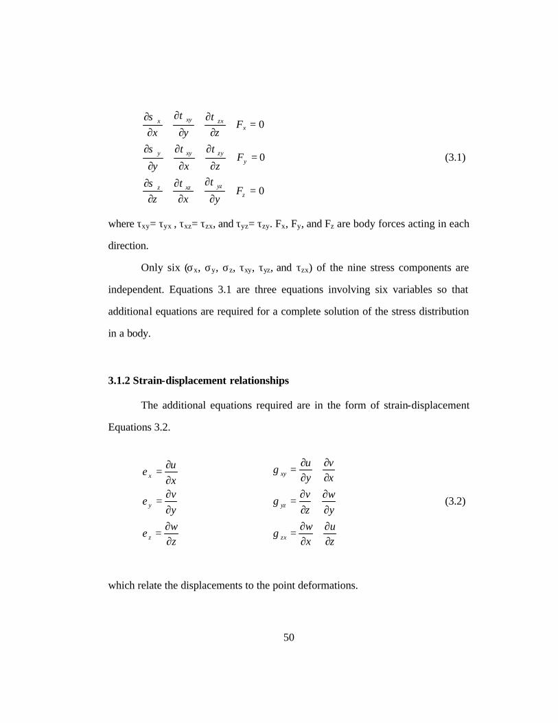
50

0

0

0

=+∂

∂+

∂∂

+∂

∂

=+∂

∂+

∂

∂+

∂

∂

=+∂

∂+

∂

∂+

∂∂

zyzxzz

yzyxyy

xzxxyx

Fyxz

Fzxy

Fzyx

ττσ

ττσ

ττσ

(3.1)

where τxy= τyx , τxz= τzx, and τyz= τzy. Fx, Fy, and Fz are body forces acting in each

direction.

Only six (σx, σy, σz, τxy, τyz, and τzx) of the nine stress components are

independent. Equations 3.1 are three equations involving six variables so that

additional equations are required for a complete solution of the stress distribution

in a body.

3.1.2 Strain-displacement relationships

The additional equations required are in the form of strain-displacement

Equations 3.2.

zwyvxu

z

y

x

∂∂

=

∂∂

=

∂∂

=

ε

ε

ε

zu

xw

yw

zv

xv

yu

zx

yz

xy

∂∂

+∂∂

=

∂∂

+∂∂

=

∂∂

+∂∂

=

γ

γ

γ

(3.2)

which relate the displacements to the point deformations.

51

3.1.3 Stress-strain relationships

Preceding sections showed two sets of equations: the equilibrium 3.1 and

the strain-displacements Equations 3.2. Equations 3.1 involve only stress

components while Equations 3.2 involve strain and displacements. This section

presents the relation between these two sets of equations.

Up to this point, material properties have not been mentioned. Establishing

a relationship between Equations 3.1 and 3.2 depends on the mechanical

properties of the particular material under consideration. For a particular medium

considered to be elastic, the equations relating stress, strain, stress-rate, and strain-

rate take the form of generalized Hooke’s law:

εσ E= (3.3)

Hooke’s law involves only stresses and strains independently of the stress-

rate or strain-rate and consists of the following equations.

( )[ ]

( )[ ]

( )[ ]yxzz

xzyy

zyxx

E

E

E

σσνσε

σσνσε

σσνσε

+−=

+−=

+−=

1

1

1

zxzx

yzyz

xyxy

G

G

G

τγ

τγ

τγ

1

1

1

=

=

=

(3.4)

52

Equations 3.5 are more common expressions of generalized Hooke’s law,

solved for stresses in terms of the strain components.

( )( )( )

zxzx

yzyz

xyxy

zyxzz

zyxyy

zyxxx

G

G

G

G

G

G

γτ

γτ

γτ

εεελεσ

εεελεσ

εεελεσ

=

=

=

+++=

+++=

+++=

2

2

2

(3.5)

Values G and λ are called Lame’s constants, and they are defined as

follows:

( )

( )( )ννν

λ

ν

211

12

−+=

+=

E

EG

(3.6)

3.1.4 Displacement formulation of problems in elasticity

The 15 Equations 3.1, 3.2, and 3.5 involve 15 variables (six stresses, six

strains, and three displacements). To handle this problem there are some reduction

procedures. Here, only the solution in terms of displacement for a three

dimensional problem is shown. It consists of three expressions in terms of

displacement.

53

By introducing Equation 3.2 into 3.5, we get six stress-displacement

relationships.

xu

Gx ∂∂

+= 2λεσ

∂∂

+∂∂

=yv

yu

Gxyτ

yv

Gy ∂∂

+= 2λεσ

∂∂

+∂∂

=xv

yw

Gyzτ (3.7)

zw

Gz ∂∂

+= 2λεσ

∂∂

+∂∂

=zu

xw

Gzxτ

=++= zyx εεεε zw

yv

xu

∂∂

+∂∂

+∂∂

(3.8)

where ε is the volumetric strain.

Combining Equations 3.7 with Equations 3.1, we have nine equations and

nine variables (six stresses plus three displacements). By introducing Equations

3.7 into 3.1, we get three equations in terms of displacements.

( ) 02 =+∇+∂∂

+ xFuGx

Gε

λ

( ) 02 =+∇+∂∂

+ yFvGy

Gε

λ (3.9)

( ) 02 =+∇+∂∂

+ zFwGz

Gε

λ

where

2

2

2

2

2

22

zyx ∂∂

+∂∂

+∂∂

=∇ (3.10)

54

3.1.5 Stresses around boreholes

Bradley (1979a) and Fjaer et al. (1992) among others present analytical

equations to compute stresses around boreholes. They assumed a state of plane

strain. This assumption simplifies the computation of stresses around boreholes

because the displacement in the direction parallel to the wellbore axis is assumed

zero (w = 0). Components u and v are function only of x and y: u=u(x,y),

v=v(x,y). Assuming plane strain, the governing equations reduce to eight: two

equilibrium equations, three stress-displacement relations, and three strain

components.

Equilibrium equations:

0

0

=+∂

∂+

∂

∂

=+∂

∂+

∂∂

yxyy

xxyx

Fxy

Fyx

τσ

τσ

(3.11)

Stress-displacement relations:

0

2

2

==

∂∂

+∂∂

=

∂∂

+

∂∂

+∂∂

=

∂∂

+

∂∂

+∂∂

=

yzxz

xy

y

x

yu

xv

G

yv

Gyv

xu

xu

Gyv

xu

ττ

τ

λσ

λσ

(3.12)

55

Strain components:

0===∂∂

+∂∂

=

∂∂

=

∂∂

=

xzyzz

xy

y

x

xv

yu

yvxu

γγε

γ

ε

ε

(3.13)

These eight equations can be reduced to two equations in terms of

displacements u and v. They are the following:

( )

( ) 0

0

2

2

=+

∂∂

+∂∂

∂∂

++∇

=+

∂∂

+∂∂

∂∂

++∇

y

x

Fyv

xu

xGvG

Fyv

xu

xGuG

λ

λ

(3.14)

Bradley (1979a) and Fjaer et al. (1992) show a set of equations in

cylindrical coordinates r, θ, z, useful to compute stress behavior around wellbores.

This set is given by Equations 3.16 that are the solution of Equations 3.14.

Stresses and strains in cylindrical coordinates relate to the cartesian coordinate

system according to the set of equations 3.15.

56

( ) ( )

θτθττ

θτθττ

θθτθθσστ

σσ

θθτθσθσσ

θθτθσθσσ

θ

θ

θ

sincos

sincos

sincoscossin

cossin2cossin

cossin2sincos

22

22

22

xzyzz

yzxzrz

xyxyr

zz

xyyx

xyyxr

−=

+=

+−=

=

−+=

++=

zw

vu

r

ru

z

r

∂∂

=

∂∂

+=

∂∂

=

ε

θε

ε

θ

1

∂∂

+∂∂

=

∂∂

+∂∂

=

∂∂

+

−

∂∂

=

zvw

r

zu

rw

rv

vu

r

z

rz

r

θγ

γ

θγ

θ

θ

121

2121

(3.15)

The derivation of the stress solution is in Jaeger and Cook (1979), and the

final equations are given by Bradley (1979a) and Fjaer et al. (1992). These are as

follows:

2

2

2

2

4

4

2

2

4

4

2

2

2sin431

2cos4312

12

rr

Prr

rr

rr

rr

rr

ww

wwxy

wwyxwyxr

+

−++

−+

−+

−

+=

θτ

θσσσσ

σ

2

2

4

4

4

4

2

2

2sin31

2cos312

12

rr

Prr

rr

rr

ww

wxy

wyxwyx

−

+−

+

−−

+

+=

θτ

θσσσσ

σ θ

( )

+−−= θτθσσνσσ 2sin42cos2

4

4

2

2

rr

rr w

xyw

yxvz

57

θτθσσ

τ θ 2cos2312sin2312 2

2

4

4

2

2

4

4

+−+

+−

−=

rr

rr

rr

rr ww

xywwyx

r

( )

++−=

2

2

1cossinrrw

yzxzz θτθττθ

( )

−+=

2

2

1sincosrrw

yzxzrz θτθττ (3.16)

where Pw is the wellbore pressure and rw is the wellbore radius.

At the wellbore wall, Equations 3.16 reduce to:

( )( )[ ]

( )0

cossin20

2sin22cos2

2sin42cos2

=

+−==

+−−=

−−−−+==

rz

yzxzz

r

xyyxvz

wxyyxyx

wr

PP

τ

θτθτττ

θτθσσνσσ

θτθσσσσσσ

θ

θ

θ

(3.17)

Although Equations 3.16 are derived form the assumption of a state of

plane strain in a linear elastic and homogeneous material, these equations are

useful to understand stress behavior around boreholes.

58

3.2 POROELASTICITY

3.2.1 Background in poroelasticity

A better mechanical properties representation for a rock formation is to

consider the existence of void space in the rock. Recently, several authors have

contributed to analyze poroelastic response of the rock under stress by developing

analytical solutions for a circular wellbore in a homogeneous and isotropic

formation, which behaves linearly and according to the poroelastic theory.

Detournay and Cheng (1988), Cui et al. (1977), and Bratli et al. (1983) solutions

are some of these. Because fluid now occupies the void space, the two

components of this new system are solid and fluid. Wang (2000) points out that

two basic phenomena underlie poroelastic behavior: Solid-to-fluid coupling and

fluid-to-solid coupling. The first occurs when a change in applied stresses

produces change in fluid pore pressure, and the second when change in fluid

pressure produces change in the volume of the porous medium.

3.2.1.1 Terzaghi’s principle

Wang (2000) among other authors points out that in general

geomechanical studies considering poroelasticity lead to Terzaghi’s formulation.

Terzaghi conducted, between 1916 and 1925, laboratory experiments on rock

samples to understand soils behavior. As a result, he derived the consolidation

equation in one-dimension for these experiments, which is analogous to the

diffusion Equation expressed in 3.18, where p is the excess water pressure, and cc

is a diffusivity factor known as consolidation coefficient.

59

2

2

zp

ctp

c ∂∂

=∂∂

(3.18)

The effective stress concept (σeff), attributed to Terzaghi, is defined as the

total stress σtotal minus formation pressure Po.

ototaleff P−= σσ (3.19)

This equation has been used extensively in rock mechanics to represent

the state of stress of a given fluid saturated porous formation.

3.2.1.2 Biot’s theory

While Terzaghi’s approach was derived in one-dimension, Biot introduced

in 1941 his three dimensional theory for poroelasticity known as “General theory

of three-dimensional consolidation”. He defined several different coefficients to

characterize rock-fluid behavior. They are known as poroelastic material

constants. By monitoring the water exchanged by flow into or out of the rock

sample, Biot defined a quantity called “variation of fluid content”, ζ. This

quantity is given by ζ=−Po/R, and it is related to the proportionality constant

called the “specific storage coefficient at constant stress”, 1/R. The second

constant refers to compressibility of the system. It is 1/H, and it is known as the

“poroelastic expansion coefficient”. The third coefficient, the drained bulk

60

modulus (K), is obtained by measuring the volumetric strain caused by applied

stress, holding the pore pressure constant.

Additional coefficients, such as Skempton’s coefficient (B) and Biot-

Willis coefficient (α), can be derived and expressed in terms of these three main

constants. Skempton’s coefficient is defined as the ratio of the induced pore

pressure to the change in applied stress for undrained conditions (ζ=0). Biot-

Willis coefficient is defined as the ratio of increment of fluid content with respect

to the volumetric strain holding the pore pressure constant. They are expressed as

follows:

( )

( )ν

εζ

α

σσσζ

213

3

0

+=

==

++−==

=

EK

HK

pHR

Bzyx

(3.20)

where ( ) 3/zyx σσσ ++ is the mean normal stress, and p is the excess water

pressure.

According to Wang (2000), the three basic material constants (1/R, 1/H,

1/K) characterize the linear poroelastic behavior of a rock-fluid system. A fourth

independent constant, shear modulus or drained or undrained Poisson’s ratio, is

required to complete the poroelastic constitutive equations when shear stresses are

present.

61

Equation 3.21 now defines the effective stress. The range for α is

1≤≤ αφ where φ is porosity. Coefficient α is less than one when the solid is

compressible (i.e., the change in volumetric strain is greater than the variation of

fluid content). When the solid is incompressible, this coefficient is exactly one

(α=1), and the Equation 3.21 simplifies to Terzaghi’s equation.

ototaleff Pασσ −= (3.21)

3.2.2 Stress-strain relationships

As in the elastic case, the poroelastic problem consists of calculating

stress, strain, and displacement components. Two new variables play a role in

poroelasticity: pore pressure and variation of fluid content in the system. Since

this procedure is analogous to elasticity analysis, the equilibrium Equations (3.1)

and the strain-displacements Equations (3.2) fully apply again. The relationship

between these two sets of equations is now modified according to Biot’s theory.

Establishing the relationship between Equations (3.1) and (3.2) in

poroelasticity depends on the coefficients defined by Biot’s theory. The

generalized Hook’s law is modified by terms that include the pore pressure of the

medium as shown in Equations 3.22.

62

( )[ ]

( )[ ]

( )[ ]

( )Rp

H

G

G

G

Hp

E

Hp

E

Hp

E

zyx

xzxz

yzyz

xyxy

yxzz

xzyy

zyxx

+++=

=

=

=

++−=

++−=

++−=

σσσζ

σγ

σγ

σγ

σσνσε

σσνσε

σσνσε

31

1

1

13

13

13

1

(3.22)

The basic variables in a three-dimensional problem in poroelasticity

include six stress components, three displacements, pore pressure and the

variation of fluid content. These eleven unknowns are solved according to eleven

equations. They are as follows. First, Equations 3.22, which include seven

equations: six stress-strain relations plus one for pore pressure. Secondly,

Equations 3.1 that are the three equilibrium equations, and finally, the diffusion

Equation 3.18 obtained by combining Darcy’s law with the continuity equation.

3.2.3 Displacement formulation of problems in poroelasticity

Analysis analogous to that done previously for elasticity is applied here to

obtain the solution in terms of displacement for a three-dimensional problem. It

consists of three expressions in terms of displacement, which include the

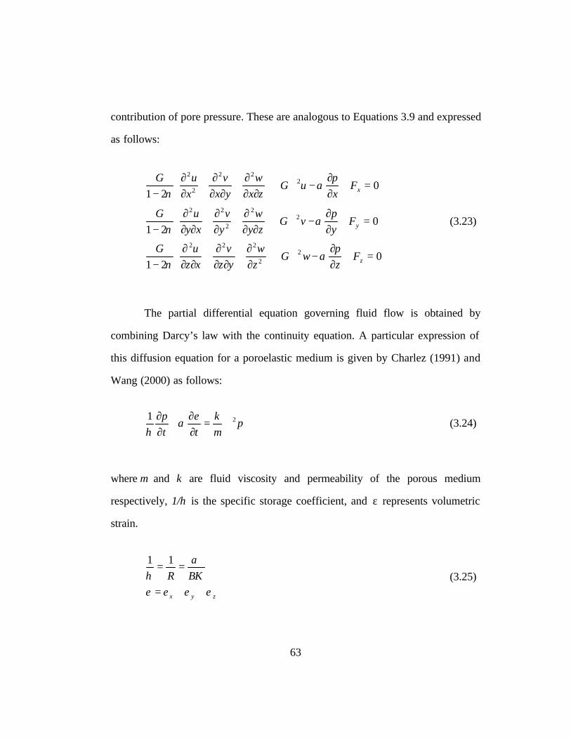
63

contribution of pore pressure. These are analogous to Equations 3.9 and expressed

as follows:

021

222

2

2

=+∂∂

−∇+

∂∂

∂+

∂∂∂

+∂∂

− xFxp

uGzx

wyxv

xuG

αν

021

22

2

22

=+∂∂

−∇+

∂∂

∂+

∂∂

+∂∂

∂− yF

yp

vGzy

wyv

xyuG

αν

(3.23)

021

22

222

=+∂∂

−∇+

∂∂

+∂∂

∂+

∂∂∂

− zFzp

wGzw

yzv

xzuG

αν

The partial differential equation governing fluid flow is obtained by

combining Darcy’s law with the continuity equation. A particular expression of

this diffusion equation for a poroelastic medium is given by Charlez (1991) and

Wang (2000) as follows:

pk

ttp 21

∇=∂∂

+∂∂

µε

αη

(3.24)

where µ and k are fluid viscosity and permeability of the porous medium

respectively, 1/η is the specific storage coefficient, and ε represents volumetric

strain.

zyx

BKRεεεε

αη

++=

==11

(3.25)

64

The term t∂

∂εα in Equation 3.24 couples the time dependence of strain

into the diffusion equation for a porous medium.

3.2.4 Stresses around boreholes

To find an analytical solution for stress distribution and displacements

around a circular wellbore in a linearly poroelastic formation even considering it

is homogeneous and isotropic requires a complex development. Among others,

particular solutions can be found in Bratli et al. (1983), Cui et al.(1997), and

Detournay and Cheng (1988). Other sources such as Fjaer et al. (1992) and

Fonseca (1998) refer also to these solutions. The original set of equations for

stress distribution in a linearly poroelastic formation where the two horizontal

stresses are isotropic can be found in Bratli et al. (1983) and appear in Fjaer et al.

(1992); they are equations presented in Equations 3.26.

65

( )

( ) ( )

( )

( ) ( )

( )

( ) ( )

−

+−−

−−

−−

−+=

−

+

+

−−−

−−

+

−−+=

+

−

−−−

−−

−

−−+=

2ln

ln

2212

21

2

1lnln

11

1221

1

ln

ln1

1221

1

022

2

22

2

2

22

2

2

22

2

2

22

2

2

22

2

ννα

νν

σνσσ

ανν

σσσ

ανν

σσσ

θ

rr

rrrr

rPP

rrr

P

rr

rrr

r

rr

rPP

rr

rrr

P

rr

rr

rr

rrr

PP

rr

rrr

P

o

w

wo

wwo

wo

wwhorvz

o

w

o

o

wo

wwo

o

wo

wwhorhor

w

o

o

o

wo

wwo

o

wo

wwhorhorr

(3.26)

It is assumed that there exists a boundary at a finite radial distance ro,

measured from the center of the wellbore. The following condition is assumed

(ro>>rw).

3.3 BOUNDARY CONDITIONS

A complete boundary value formulation consists of the governing

equations and the boundary conditions. The boundary conditions applicable to the

stress-displacement Equation 3.23 and to the diffusion Equation 3.24 depend on

66

the physical phenomenon analyzed. Chapter 4 presents the assumptions to attempt

simultaneous solutions for stress-displacement and pore pressure distribution in

the physical problem considered in this study. The choice of boundary conditions

is made among the following:

1) Essential boundary conditions: The value of the dependent variable is

specified at the boundary.

In the case in which the displacement components are prescribed over

the entire boundary, the boundary conditions for the stress-displacement

Equation 3.23 are expressed as follows:

( ) utzyxu =,,, : ( ) vtzyxv =,,, : ( ) wtzyxw =,,, (3.27)

For the diffusion Equation 3.24, the essential boundary condition is

pore pressure prescribed over the boundary. In this case, the boundary

condition for the diffusion Equation 3.24 is the following:

( ) ptzyxp =,,, (3.28)

2) Natural boundary conditions: The value of the first derivative of the

dependent variable is prescribed at the boundary.

The boundary conditions for the stress-displacement Equation 3.23 are

the following where the stress, σ , is prescribed over the entire boundary:

67

( ) σ=∇ tzyxuE ,,, : ( ) σ=∇ tzyxvE ,,, : ( ) σ=∇ tzyxwE ,,, (3.29)

For the diffusion Equation 3.24, the boundary conditions are given by

the flow rate, q, specified at the boundary.

( ) qtzyxpk

=∇ ,,,µ

(3.30)

In Chapter 4, it is shown that the complete boundary value formulation of

the physical problem is stated in terms of a combination of the boundary

conditions here presented. Essential boundary conditions are specified at the outer

boundaries for both the stress-displacement and the diffusion equations. Natural

boundary conditions are prescribed at the inner boundary for both equations.

Becker et al. (1981) define this kind of problem as a mixed boundary-value

problem. The physical meaning of imposing these particular boundary conditions

is fully explained in Chapter 4.

3.4 SWITCHING FROM A BOUNDARY VALUE PROBLEM TO WELLBORE STABILITY ANALYSIS

The boundary value formulations stated in this chapter allow finding the

solution for stress and strain around wellbores. This solution is completely

dependent on the constitutive model applied to the analysis. The connection

between these boundary value formulations and wellbore stability analysis is

given by a failure criterion. Different kinds of failure criteria were mentioned in

68

the last chapter. They range from the simplest peak-strength criterion to complex

criteria based on a failure surface. In addition, wellbore closure is being recently

considered as a criterion to determine wellbore instability. These failure criteria

will be used to analyze and discuss wellbore stability in Chapter 5.

69

Chapter 4: Numerical Approach to the Solution of the Wellbore Stability Problem

The review of literature in Chapter 2 discusses the status of the study of

wellbore stability around the junction in multilateral wells and concludes that the

current trend towards analyzing this problem is by implementing numerical

solutions in 3-D. Finite element techniques have proven to be reliable in areas

such as aerospace and structure analysis. As a result of this success, researchers

have turned their attention to use finite element theory in modeling

geomechanical problems and recently in wellbore stability analysis. This chapter

serves to support the decision of using commercial finite element software to

conduct this investigation. The second major part of this chapter presents the

mathematical representation of the physical phenomena studied.

4.1 COMPUTATIONAL MODELING

According to Starfield and Cundall (1988), by comparing rock mechanics

problems with other areas of mechanics such as aerospace or structural

mechanics, rock mechanics modeling falls into the class of problems dealing with

limited amount of data. This leads to the question of why mathematical or

computational models are considered viable tools to forecast the behavior of rock

in the absence of enough information. One of the reasons to think about

computational modeling to simulate rock mechanic problems is accessibility to

more versatile and powerful computer packages that have been successfully

applied in other areas. As a consequence of this versatility, these computer

70

packages have increased their ability to handle geological detail in construction of

appropriate models. Easy access to high-performance computers provides to the

modeler an important tool. Although the limited amount of geological data is a

concern in modeling process, it is necessary to accept and recognize that to

reproduce real events; it should be necessary to construct a model with the same

complexity as reality. An alternative to overcome this situation is simplifying the

model by applying appropriate assumptions.

4.1.1 Analytical and Numerical solutions

The main aspects that support the decision of working with numerical

methods are founded on the statements of researchers who support numerical

simulation. Hibbit, Karlsson, and Sorensen (2000a) state that all physical

phenomena behave non- linearly and the three different sources of non-linearity

are due to material, boundary conditions, and geometry.

The first type of nonlinear problem is associated with material properties.

As mentioned in Chapter 2, for unconsolidated sands and shales there is not

enough cohesion between grains, and only a consolidation deformation

mechanism exists. According to Chen et al. (2000), to estimate displacements and

changes in stress distribution for these materials, non-linear constitutive models

should be considered. Chen agrees with Charlez (1997a) by stating that two

conditions are required to obtain an analytical solution from a given initial

boundary value problem in elastoplasticity. First, the shape of the plastic zone

must be known in advance to couple the elastic equations with the corresponding

71

ones for the plastic zone. Charlez stated that although for an isotropic initial stress

field the shape of the plastic zone can be known, for an anisotropic stress field this

shape remains unknown, and only numerical approaches can be applied to find a

solution. The second requirement is that the constitutive models representing

material behavior for the elastic and the plastic zones must be expressed linearly

in order to superpose their solutions. Other sources of non-linear behavior related

to material properties are for materials exhibiting either strain-rate dependence or

post-failure behavior.

The second source of non- linearity is due to boundary conditions. When

boundary conditions change during a particular analysis, non- linearity occurs. For

instance, in hydraulic diffusion analysis, boundary conditions may change from

no-flow condition to flow condition. This change causes variations in pore

pressure, which are time dependent. This phenomenon can be properly

incorporated numerically.

The third source is related to changes in the geometry of a body during a

given analysis. Necas and Hlavacek (1981) pointed out that the concept of “small

strain tensor”, defined in classical mechanics, raises the question of when a given

strain tensor represents the real deformation of the body. Hibbit, Karlsson, and

Sorensen (2000a) explain that when a problem is defined as a “small-

displacement” analysis, the problem is linearized, ignoring any possible geometric

nonlinear response. The alternative to a “small-displacement” analysis is to

include “large-displacement” effects. This alternative allows taking into account

the geometric non-linear response of the body.

72

Because some of the sources of non- linearity mentioned before are

expected in the physical phenomenon studied in this research, a numerical

approach arises as the most likely tool to attempt a solution.

Selection of a constitutive model is not arbitrary. As many of the

researchers in wellbore stability mention, strictly there will always be a need to

compare the model predictions against laboratory data and calibrate the model if

possible. ABAQUS version 6.2, developed by Hibbit, Karlsson, and Sorensen

(2000a), is a finite element software developed initially to study problems related

to structural analysis. Because of its success, it has become a general purpose

modeling software package. ABAQUS is equipped to handle different constitutive

models to represent material behavior, and as such, it was chosen as the

commercial finite element software to conduct this research.

4.2 CONSTITUTIVE MODELS AVAILABLE IN ABAQUS

In former chapters, it was mentioned that the solution to a particular

boundary value problem depends on the constitutive model used in the analysis.

Since ABAQUS is a general purpose finite element software, it allows

considering different constitutive models. These models range from the purely

elastic model, passing through models that take into account void ratio such as

poroelasticity to complex models that incorporate plasticity. Elastoplastic models,

particularly those based on the theory of critical state introduced by Roscoe and

Burland during the 1960’s at Cambridge, are considered good tools to reproduce

shales behavior. In order to analyze and compare rock behavior with respect to the

73

constitutive model, we discuss the following constitutive models: elastic,

poroelastic, and poroelastoplastic.

For the simplest case of elasticity, Young’s modulus and Poisson’s ratio

are the required parameters. If a porous medium is considered, then in addition to

the elastic parameters, the following parameters are required: bulk modulus of

rock and fluid, shear modulus, average rock porosity and average rock

permeability, densities of rock and fluid contained.

Two different elastoplastic models are addressed: Drucker-Prager and

Cam-Clay. These models are described by Hibbit, Karlsson, and Sorensen

(2000a). For these models, in addition to the information mentioned above,

hardening and post-failure behaviors of rock are required. The results of a triaxial

compression test are required to calibrate the Drucker-Prager model. Two tests are

required to calibrate the Cam-Clay model: a hydrostatic compression test and a

triaxial compression test.

For the Cam-Clay model, laboratory test results must be expressed in

terms of critical state variables. The hydrostatic compression test consists of

applying equal compression forces in all directions to a rock sample. This test

provides the initial shape of the yield surface, a0.

−−−

=ss

s

kpkee

aλ

0010

lnexp

21

(4.1)

where e1 is defined by the intersection of the consolidation line with the void ratio

axis as shown in Figure 4.1 while e0 is the void ratio measured at the beginning of

74

the test. The logarithmic bulk modulus λs, and the swelling coefficient κs

represent the slopes of the consolidation line and the swelling line respectively.

p’:q’ were defined in Equations 2.7 in Chapter 2.

Void ratio, e, is related to the measured volume change as follows:

( )01

1exp

ee

++

=ε (4.2)

Details of the methodology of each test can be found in Atkinson and

Bransby (1978). Briefly, a compression test consists of measuring the volume of

water expelled from the sample at different confining pressures, p’. Specific

volume values v are obtained from the relative density Gs and water saturation Sw

of the sample swGSe +=+= 11v . On the other hand, a triaxial test allows the

calibration of the yield parameter M, which is defined as the slope of the critical

state line on the p’:q’ plane.

4.3 MODEL DEFINITION

4.3.1 Model’s geometry for analysis in a single hole

A 3-D finite element model (FEM) constructed using hexahedral elements

was used to predict the behavior of rock formation surrounding a single wellbore

whose diameter is 8 ½ inches (0.21596 m). Because the initial state of stress is

altered over a distance of 5 to 7 times the wellbore radius, the model consists of a

square region of 3.0 by 3.0 meters, which is equivalent to 15 radii. It helps to

75

represent better the boundary conditions at infinity. Figure 4.2 illustrates the

model.

Mesh refinement calculations were done to assure accuracy of the results.

Figures 4.3 and 4.4 show results of mesh refinements for the radial and tangential

directions using equally spaced quadratic elements. Rock is assumed to be elastic

with the following properties: E=10000 MPa and ν=0.30. The analysis assumes a

plane stress condition for a vertical wellbore of radius equal to 0.1 meters in a

stress field σx=σy=10 MPa. Wellbore pressure imposed is Pw=7 MPa. Figure 4.3

shows the radial stress as a function of radial distance varying the number of

equally spaced quadratic elements in the radial direction (Nr). The results are

compared with the analytic elastic solution. It can be seen how the accuracy of the

results increases significantly as Nr increases from 7 to 28 elements. This plot

shows that accuracy of the results is highly sensitive to mesh size in the radial

direction. The relationship between the size of the element and the number of

elements in the radial direction (Nr) is as follows: element size=0.164 m. for

Nr=7, element size=0.082 m. for Nr=14, and element size=0.041 m. for Nr=28.

These results show that to obtain accuracy in results, the size of the equally

spaced quadratic elements in the radial direction must be equal or smaller than

0.041 m. Figures 4.4 and 4.5 illustrate the radial and the tangential stresses,

respectively, as a function of radial distance varying the number of quadratic

elements in the tangential direction (Nθ) from 8, 16, 32, and 64. Because all the

curves in both Figures 4.4 and 4.5 converge to a single curve, it can be concluded

76

that mesh size in the tangential direction does not affect accuracy of the results for

the radial and tangential stresses in the range of Nθ values analyzed.

Figure 4.3 also shows that the initial state of stress is altered over a

distance of 5 to 7 times the wellbore radius. Beyond this zone, the solution tends

to the initial conditions. In order to improve the accuracy of the results in the

nearest region to the wellbore, a denser concentration of “unequally spaced”

quadratic elements was applied instead of “equally spaced” quadratic elements.

Figure 4.6 shows these results.

4.3.2 Drilling simulation in a single hole

Traditional stress-displacement analyses assume the wellbore has been

previously drilled. It is assumed that a cylindrical hole preexists when the analysis

is performed. In contrast, this model allows simulation of the process of drilling in

sequential steps. A cylindrical hole also exists in this model, which constitutes the

wellbore, but in order to simulate as close as possible the process of drilling a

sequence of steps is followed. The first step of a given analysis consists of trying

to equilibrate geostatic forces acting on the system. Secondary steps simulate the

process of drilling. There are three different strategies to find initial equilibrium

and to simulate drilling.

The first strategy follows Hibbitt, Karlsson, and Sorensen (2000b)

methodology when they simulated tunnel excavations. It consists of applying,

during the first step, concentrated loads at the nodes located in the wellbore wall

(inner boundary). These loads must be in equilibrium with the initial stress field,

77

and they are applied as reaction fo rces to restore as close as possible the state of

stress existing before drilling. To do that, it is necessary to determine from a

previous independent analysis the magnitude and location of these loads, and then

add them to the model manually at the correct nodes of the wellbore wall. Once

these loads are applied and equilibrium is achieved during the first step, drilling

process simulation begins in a second step by reducing those loads to a value of

well pressure desired, one layer at a time until the wellbore penetration is

achieved. This procedure is tedious for fine meshes or large models such as those

defined in Sections 4.3.1 and 4.3.3 and illustrated in Figures 4.7 and 4.8 in this

Chapter 4. Therefore, this strategy is unpractical and a second and simpler

approach may be used.

The second strategy consists of applying during the initial step; instead of

concentrated loads at nodes, distributed loads on the wellbore wall. These

distributed loads are in equilibrium with the initial stress field and equivalent to

pressure applied inside the wellbore. Again, once equilibrium is achieved, the

second step consists of reducing those loads to a value of well pressure desired. It

solves the problem of adding loads manually to the model, which was mentioned

before for fine or large meshes. When a highly anisotropic initial stress field

exists, an independent analysis has to be done in order to estimate the internal

wellbore pressure required to equilibrate the model, and then apply this pressure

as a distributed load on the wellbore wall.

The third alternative is using what in theory is known as “ghost” elements.

This strategy is based on filling the wellbore with additional “ghost” elements. In

78

this way, the model does not require any load at the inner boundary to find

equilibrium. Deactivating those “ghost” elements that represent drilled rock, by

reducing their stiffness to negligible values simulates the drilling process. Then,

fluid pressure inside the wellbore is applied in the form of distributed loads on the

wellbore wall. In this case, since the “ghost” elements are deactivated during the

drilling step, it is necessary to be careful about boundary conditions and any kind

of nodal forces applied to the surfaces that are in contact with those “ghost”

elements.

To simulate drilling in a single step, the model consists of (28x64x1) 1792

hexahedral elements and 12864 nodes and uses a single thin 0.05 meters layer, as

shown in Figure 4.2. In order to keep the aspect ratio of the hexahedral elements,

it is recommended that the size of the layer in the vertical direction be in accord

with the size of the elements in the radial direction. On the other hand, to simulate

drilling in a multi-step process, the model uses ten layers, and it consists of

(28x16x10) 4480 hexahedral elements. This kind of model is defined as a “multi-

layer model”. Figure 4.7 illustrates this case.

4.3.3 Model’s geometry for analysis in a multilateral scenario

A totally different 3-D finite element model shown in Figure 4.8 was

constructed by using the pre-processor ABAQUS/CAE for simulation of the

lateral junction. The dimensions and characteristics of the model are as follows.

The mainbore diameter is 12 ½ inches (0.31758 m), and the lateral wellbore

diameter is 8 ½ inches (0.21956 m). The lateral wellbore is constructed in the

79

direction of the “σx” principal stress with an inclination of 2.5o. Considering the

junction angle equal to 2.5o, the height of the window created in the mainbore is

about 5.05 meters long. It is an axis-symmetric rectangular region 1.2 by 0.4 by

8.0 meters, consisting of 14816 hexahedral quadratic elements and 68575 nodes.

Figure 4.9 shows a closer view of this model. This representation was chosen

after several attempts using different model dimensions. The initial dimensions of

the model were 3.0 by 1.5 by 8.0 meters. However, the computer used to carry out

the analysis was unable to handle the finite element code needed to perform the

numerical calculations of this model; therefore, resizing of the model was done to

allow execution of the code. By doing this resizing, the computing problems were

solved. Section 5.2.1.1 in Chapter 5 will show how this resizing causes alteration

of the stress behavior in the region near to the boundaries, but it does not affect

the stress behavior in the region between the holes where instabilities are expected

due to the presence of the lateral well.

4.3.4 Drilling simulation in a multilateral scenario

The purpose of this research is to observe the influence of drilling a

second hole from the mainbore. Simulation of drilling can also be done in a single

or multiple step analysis like in the situation of a single hole. Some restrictions

apply for drilling simulation process in a multilateral scenario. Drilling simulation

of the lateral wellbore for the multilateral case considers that the mainbore was

drilled previously, and it exists at the time the lateral wellbore is being drilled.

Because of the complexity and large number of nodes and elements required in

80

constructing a model involving a multilateral scenario, only the second strategy

previously described is applicable to simulate the drilling of the lateral well. This

strategy consists of applying, during the initial step, distributed loads on both

wellbore walls the mainbore wall and the lateral wall. Initially, distributed loads

applied at the wellbore wall of the lateral well are in equilibrium with the initial

stress field while distributed loads applied at the wellbore wall of the mainbore

represent hydrostatic pressure created by the drilling fluid. The second step

consists of reducing the loads applied at the lateral wellbore wall to a wellbore

pressure value equal to the wellbore pressure imposed at the mainbore.

4.4 WELLBORE STABILITY MATHEMATHICAL MODEL

This section presents the assumptions and equations to compute stress

distribution and displacements around wellbores. Conventional stress analysis is

fully coupled with fluid flow equations to attempt simultaneous solutions for

stress/displacement and pore pressure distribution.

4.4.1 General assumptions

General assumptions are as follows:

• Static equilibrium (No inertial forces acting).

• It is accepted that the model represents rock formation.

• Rock formation is homogeneous.

• Temperature remains constant during each particular analysis.

81

• The axes of the global coordinate system are parallel to the in-situ

principal stresses.

• Mass diffusion process is not taken into account.

4.4.2 Governing equations

Chapter 3 presented the governing equations involved in the solution of a

general stress-displacement problem in elasticity and poroelasticity. The final

governing equation depends on the constitutive model considered. In general, the

final governing equation can be written in vector form as follows:

0CBA 2 =+∇+∇+⋅∇∇ kFpUU (4.3)

where A, B, and C are material constants, and Fk represents body forces assuming

negligible inertial effects.

Diffusion processes occur in porous media. Three different diffusion

processes can be identified affecting wellbore stability. They are pore pressure

diffusion associated with hydraulic conductivity of rocks, thermal diffusion, and

mass diffusion process related to ions exchange between formation fluids and

drilling mud. This last is recognized as the chemical effect.

According to Charlez (1991) and Wang (2000), the first of these three

processes can be mathematically represented by the diffusion Equation 4.4. In this

equation, 1/η is the specific storage coefficient, ε represents volumetric strain

82

defined by the bulk volume variations, α is Biot’s coefficient, and L is called

latent heat. This diffusion equation coupled with the Equation 4.3 describes a

wellbore stability problem considering hydraulic diffusivity.

pk

tT

TL

ttp 21

∇=∂∂

−∂∂

+∂∂

µηρε

αη

(4.4)

Lomba et al. (2000a) developed a model to calculate the transient pressure

profiles and solute diffusion through low permeability shales. The solute

concentration profile is defined according to the mass diffusion equation:

seffs CD

tC 2∇=∂

∂ (4.5)

where Cs is the concentration of solute, and Deff is the diffusivity of the diffusing

material.

They found that both hydraulic and mass diffusion processes induce the

flow of solute and water. The coupled equation to represent these phenomena is

expressed by Lomba et al. (2000a) as follows:

sf

II

f

I Cc

nRTKp

cK

tp 22 ∇=∇−

∂∂

(4.6)

83

In this equation, IK was defined as hydraulic diffusivity and fc is fluid

compressibility while f

II

cnRTK

represents diffusivity.

The mathematical relationship that describes a problem considering both

hydraulic and mass diffusion processes can be obtained from the Equations 4.4

and 4.6 and expressed as follows:

sf

II

f

I Cc

nRTKp

cK

tT

TL

ttp 221

∇+∇=∂∂

−∂∂

+∂∂

ηρε

αη

(4.7)

Hence, to describe a wellbore stability problem in elasticity and

poroelasticity, the stress-displacement formulation given by Equation 4.3 couples

with Equation 4.7. Because ABAQUS version 6.1 is no t equipped to couple both

the hydraulic and the mass diffusion processes with the stress-displacement

problem, the pore pressure alteration induced by chemical potential cannot be

quantified.

4.4.2.1 Isothermal analysis

Taking into account the general assumptions stated in Section 4.4.1, we

obtain the following for the particular case of an isothermal analysis, where

0=∂∂

tT

TL

ηρ

(4.8)

84

Equation 4.7 reduces to:

sf

II

f

I Cc

nRTKp

cK

ttp 221

∇+∇=∂∂

+∂∂ ε

αη

(4.9)

4.4.2.2 Hydraulic diffusion analysis

Because hydraulic diffusivity is the diffusion process addressed in this

research, the second term in the right hand side of the Equation 4.9 becomes zero,

and the Equation 4.9 reduces to the following.

pcK

ttp

f

I 21∇=

∂∂

+∂∂ ε

αη

(4.10)

Both Equation 4.3 and Equation 4.10 constitute the mathematical

representation of the physical phenomena studied in this research.

4.4.3 Phenomena in steady state

4.4.3.1 Stress-displacement analysis in Elasticity

The simplest case to analyze is to consider a rock formation, which

behaves according to the linear elastic theory. In addition to the general

assumptions stated in Section 4.4.1, these other assumptions are required:

85

• Rock’s porosity is negligible such that the influence of fluid

contents on rock behavior is not taken into account.

• Rock’s behavior can be modeled as a perfect elastic material.

• Because porosity is assumed negligible, diffusive processes do not

occur.

• No time dependent effects are involved (i.e., the rate of

deformation is independent of the rate of loading).

Because of these assumptions, all the terms in Equation 4.10 vanish, and

the Equation 4.3 constitutes the mathematical representation this stress-

displacement problem. In this case, Equation 4.3 is rewritten as follows:

( ) 02 =+∇+⋅∇∇+ kFUGUGλ (4.11)

where the material constants A, B, and C have been substituted.

( )

0CBA

==

+=G

Gλ

Equation 4.11 is the vector form of Equations 3.9 derived in Chapter 3,

which are rewritten in Equations 4.12

86

( ) 02 =+∇+∂∂

+ xFuGx

Gε

λ

( ) 02 =+∇+∂∂

+ yFvGy

Gε

λ (4.12)

( ) 02 =+∇+∂∂

+ zFwGz

Gε

λ

Boundary conditions.

The first alternative to represent boundary conditions at far field is by

using what in ABAQUS is defined as infinite elements. Hibbitt, Karlsson, and

Sorensen (2000a) suggest that these infinite elements can be used in conjunction

with finite elements in boundary value problems defined in unbounded domains

where the region of interest is relatively small compared to the surrounding

medium. Infinite elements were applied at far field in the model; however, the

computer used to perform the analysis was unable to handle the finite element

code needed to perform the numerical calculations due to memory capacity.

Therefore, a second alternative was assumed, which solved the problem. This

second alternative consisted of specifying the magnitudes of the displacements at

far field equal to zero. Equations 4.13 give these boundary conditions.

( )( )( )

0),,(

0,,0,,

0,,

==

====

==

bbbb

bbbb

bbbb

bbbb

UzyxUor

wzyxwvzyxv

uzyxu

(4.13)

87

The boundary condition at the wellbore wall is given by the first derivative

of the displacements. Stress is specified at this boundary and represented by

Equation 4.14.

wooo PzyxUE =∇ ),,( , (4.14)

where E is Young’s modulus representing the material properties, and Pw is the

wellbore pressure.

4.4.3.2 Stress-displacement analysis in Poroelasticity

To perform this kind of analysis, in addition to the general assumptions

imposed in Section 4.4.1, the following assumptions are required.

• A single fluid saturates the porous medium.

• Drilling fluid (mud) creates a membrane on the wellbore wall

representing filter cake. Permeability of this membrane is low

enough to be neglected. The filter cake is assumed impermeable.

• Mass diffusion (chemical interaction) is neglected under the

assumption that the filter cake acts as a perfect barrier impeding

filtrate to invade formation. Under this condition, it is assumed that

in-situ formation fluids do not get into contact with the drilling

fluid. This condition avoids ion exchange into or out the formation,

and chemical interaction between fluids can be neglected.

88

• No time dependent effects are involved (i.e., the rate of

deformation is independent of the rate of loading).

Because of these assumptions, all the terms in Equation 4.10 vanish, and

Equation 4.3 constitutes the mathematical representation of the stress-

displacement problem in poroelasticity. In this case, Equation 4.3 is written as

follows:

021

2 =+∇−∇+⋅∇∇− kFpUGUG

αν

, (4.15)

where the material properties are expressed as follows:

α

ν

−==

−=

CGB

GA

21

In expanded form, Equation 4.15 is written as follows:

021

222

2

2

=+∂∂

−∇+

∂∂

∂+

∂∂∂

+∂∂

− xFxp

uGzx

wyxv

xuG

αν

021

22

2

22

=+∂∂

−∇+

∂∂

∂+

∂∂

+∂∂

∂− yF

yp

vGzy

wyv

xyuG

αν

(4.16)

021

22

222

=+∂∂

−∇+

∂∂

+∂∂

∂+

∂∂∂

− zFzp

wGzw

yzv

xzuG

αν

89


The boundary conditions are given by Equations 4.13 and 4.14 as stated

before.

4.4.4 Transient phenomena

Until recently, wellbore stability had been mainly analyzed as a steady-

state phenomenon. The review of literature in Chapter 2 showed that most authors

actually recognize wellbore instability as a time dependent problem. Charlez

(1997a) classifies these time dependent problems in two categories. First,

deformation and rupture in rocks exhibiting plastic behavior. Second, diffusion

processes through porous medium.

4.4.4.1 Rate of Deformation

Multi step drilling analysis (MSDA) has the purpose of simulating the first

of these effects, material deformation as a function of time, rate of deformation.

To achieve this, rather than considering that the borehole is drilled

instantaneously, MSDA considers the process of drilling in sequential steps. This

condition gives the model the opportunity of behaving as function of time. Each

step in an analysis is divided into multiple increments. The user defines the total

time of each step and suggests the first time increment. Then ABAQUS controls

automatically time increments during a step to obtain a solution in the least

90

possible computational time. These time increments depend on the severity of the

nonlinear response of each particular problem.

Because this kind of analysis is based on a “multi- layer model”, drilling

process can be simulated in several drilling steps according to the number of

layers. The multi- layer model and the simulation of the drilling were described in

Section 4.3.2.

In order to set mathematically this problem, these other assumptions are

considered in addition to the general assumptions defined in Section 4.4.1:

• Rock’s porosity is negligible such as the rock behaves as a solid.

• Rock’s behavior obeys to an elastoplastic constitutive relationship.

• Because porosity is assumed negligible, diffusion processes do not

occur.

As a consequence of these assumptions, the only term remaining in

Equation 4.10 is the coupled term representing the rate-dependent deformation

behavior of the material, which is given according to the equation:

twr ∂

∂=

ε (4.17)

Because an elastoplastic model is being used to carry out the analysis for

this particular case, stress-strain relationships are nonlinear. Equation 4.3 is no

longer applicable because of plastic material properties. In order to set up this new

91

problem, rather than defining the problem in terms of differential equations,

variational principles for energy are applied.

Necas and Hlavacek (1981) and Doltsinis (2000) define a stress-strain

problem of equilibrium in terms of the principle of virtual work for a static stress

field σ as follows. “The virtual work of the internal forces (left hand side of

Equation 4.18) equals the virtual work of the external forces, which are body

forces per unit volume f at any point within the material V plus surface tractions

per unit area t on the surface S bounding this volume (right-hand side).” Equation

4.18 represents a complete statement of the stress-strain problem of equilibrium in

terms of displacements in three-dimensions.

∫ ∫∫ ⋅+⋅=

V SVvdStvdVfDdV δδδσ : , (4.18)

where Dδ is defined as a virtual rate of deformation, and vδ is a virtual velocity

field.

This equation is the basic equilibrium statement for the formulation of a

problem in the finite element theory. Equation 4.18 coupled with Equation 4.17

represents the physical phenomenon of stress behavior and deformation in rocks

exhibiting plastic behavior.

Initial conditions.

This is given according to the strain rate dependence of the material.

92

0)0,,,( εε =zyx (4.19)


The boundary conditions are given by Equations 4.13 and 4.14.

4.4.4.2 Coupled stress-hydraulic diffusion analysis

Another cause of wellbore instabilities associated with time is the fluid

diffusive process through a porous medium. In order to observe the response of a

porous formation, Charlez (1997a, 1997b) proposed the simulation in two

different steps, which must be carried out successively. The first step is a

simulation of the drilling process, which consists in decreasing the pressure

applied in the wellbore. The second step simulates the hydraulic diffusion

response of the porous medium.

In order to set this problem mathematically, in addition to the general

assumptions defined in Section 4.4.1, these assumptions are required:

• A single fluid saturates the porous medium.

• The drilling fluid (mud) creates an impermeable membrane on the

wellbore wall (filter cake). Under this condition, hydraulic

diffusion is allowed within the system, but mass diffusion

(chemical interaction) is neglected. Because the filter cake acts as

a perfect barrier impeding filtrate to invade formation, it is

93

assumed that in-situ formation fluids do no get into contact with

the drilling fluid. This condition avoids ion exchange into or out

the formation, and chemical interaction between fluids can be

neglected.

Equation 4.10 fully applies to this case, and it is rewritten in Equation

4.20.

pcK

ttp

f

I 21∇=

∂∂

+∂∂ ε

αη

(4.20)

Equation 4.20 coupled with Equation 4.18 constitutes the mathematical

representation of the coupled stress-hydraulic diffusion problem.

Initial conditions.

( ) 0

0

0,,,)0,,,(

εε ==

zyxpzyxp

(4.21)


Conditions during the drilling step at the inner and the outer boundaries

are respectively specified in Equations 4.22 and 4.23. Due to the existence of the

94

filter cake, no flow condition at the wellbore wall is imposed. It is represented by

Equation 4.22.

( ) 0,,, =∇ tzyxpk

oooµ (4.22)

Because the outer boundary is assumed at a finite distance far away from

the wellbore, ro, a pressure boundary condition, Equation 4.23, is prescribed at

this boundary. This equals the initial pore pressure of the porous medium.

( ) obbb ptzyxp =,,, (4.23)

4.5 SOLUTION METHOD USED IN ABAQUS

Hibbitt, Karlsson, and Sorensen (1998) give a complete description of the

formulation of a strain-stress finite element analysis. This section only describes

the basics of this formulation.

Equilibrium in terms of the principle of virtual work is defined according

to the following equation.

∫ ∫∫ ⋅+⋅=V SV

vdStvdVfDdV δδδσ : (4.24)

For a porous medium, body forces f include the weight of total liquid

contained, fw.

95

( ) gSf wtww ρφφ += (4.25)

The term ( )twS φφ + in Equation 4.25 includes the fraction of water that is

free to move through the porous medium, φwS , plus the volume of irreducible

water per unit of total volume, tφ . Sw is the water saturation that is free to move,

pww VVS = . φ is porosity, bp VV=φ . wρ is water density, and g is the

gravitational acceleration.

Because IN represents the internal forces and PN represents the external

forces, the virtual work equation can be rewritten as Equation 4.26.

0=−

=NN

NN

PI

PI (4.26)

where IN and PN are respectively.

∫ ∫∫

⋅+⋅=

=

V S

N

V

N

vdStvdVfP

DdVI

δδ

δσ : (4.27)

When Equation 4.27 is discretized in terms of the virtual velocity field vδ

and the virtual rate of deformation Dδ , the resultant system of equations forms

the basis of a finite element analysis. It can be expressed in the following form.

( ) 0=NN xF (4.28)

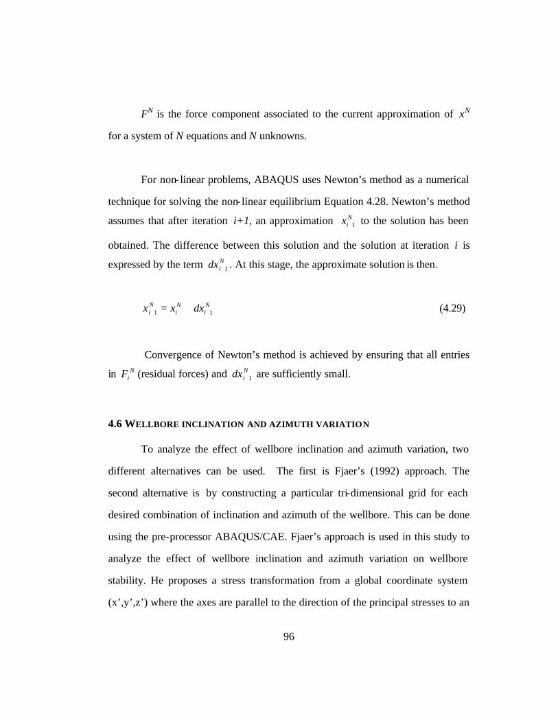
96

FN is the force component associated to the current approximation of xN

for a system of N equations and N unknowns.

For nonlinear problems, ABAQUS uses Newton’s method as a numerical

technique for solving the nonlinear equilibrium Equation 4.28. Newton’s method

assumes that after iteration i+1, an approximation Nix 1+ to the solution has been

obtained. The difference between this solution and the solution at iteration i is

expressed by the term Nidx 1+ . At this stage, the approximate solution is then.

Ni

Ni

Ni dxxx 11 ++ += (4.29)

Convergence of Newton’s method is achieved by ensuring that all entries

in NiF (residual forces) and N

idx 1+ are sufficiently small.

4.6 WELLBORE INCLINATION AND AZIMUTH VARIATION

To analyze the effect of wellbore inclination and azimuth variation, two

different alternatives can be used. The first is Fjaer’s (1992) approach. The

second alternative is by constructing a particular tri-dimensional grid for each

desired combination of inclination and azimuth of the wellbore. This can be done

using the pre-processor ABAQUS/CAE. Fjaer’s approach is used in this study to

analyze the effect of wellbore inclination and azimuth variation on wellbore

stability. He proposes a stress transformation from a global coordinate system

(x’,y’,z’) where the axes are parallel to the direction of the principal stresses to an

97

orthogonal local coordinate system (x,y,z) where the z-axis is parallel to the axis

of the borehole. The global coordinate system (x’,y’,z’) is oriented so that the x’-

axis is parallel to the maximum horizontal stress σH, y’-axis is parallel to the

minimum horizontal stress σh, and z’-axis is parallel to the vertical stress σv.

Figure 4.10 shows this coordinate system transformation for a deviated well.

This transformation is expressed by using the direction cosines which

depend on the azimuth “a” and the wellbore inclination “i”. To transform from the

(x’,y’,z’) to the (x,y,z) coordinate system, the azimuth “a” is defined as the angle

between the x’-axis and the projection of the x-axis on the (x’:y’) plane while the

inclination “i” is defined as the angle between the z’-axis and the z-axis. The

direction cosines matrix [l], and the transformation of the in-situ stress tensor [σ’]

from the global to the local frame [σ0] are given by the following equations.

[s 0] = [l] [s’] [l]T

where

−

−

=iiaia

aa

iiaia

lcossinsinsincos0cossin

sincossincoscos

][

=

v

h

H

σσ

σ

σ00

00

00' (4.30)

=ozz

ozy

ozx

oyx

oyy

oyz

oxz

oxy

oxx

o

σττ

τστ

ττσ

σ

98

The final expressions are as follows:

ial xx coscos' = al yx sin' −= ial zx sincos' =

ial xy cossin' = al yy cos' = ial zy sinsin' = (4.31)

il xz sin' −= 0' =yzl il zz cos' =

Expressed in the (x, y, z) coordinate system, the in-situ stresses σH, σh,

and σv become:

vxzhxyHxxox lll σσσσ ''' 222 ++=

vyzhyyHyxoy lll σσσσ ''' 222 ++=

vzzhzyHzxoz lll σσσσ ''' 222 ++=

vyzxzhyyxyHyxxxoxy llllll σσστ ''''' ++= (4.32)

vzzyzhzyyyHzxyxoyz llllll σσστ ''''' ++=

vxzzzhxyzyHxxzxozx llllll σσστ ''''' ++=

99

Figure 4.1 Pure compression behavior of clay (from ABAQUS/Standard User’s manual, Version 6.1, 2000).

e1 = locates initial consolidation state @ lnp’=0

-ks = slope of swelling line

-λs = slope of consolidation line

ln p’

e

100

Figure 4.2. Model mesh for a single hole one step.

101

Figure 4.3 Effect of mesh refinement in the radial direction on the accuracy of radial stress calculations.

Figure 4.4 Effect of mesh refinement in the tangentia l direction on the accuracy of radial stress calculations.

6.5

7.0

7.5

8.0

8.5

9.0

9.5

10.0

10.5

0 0.2 0.4 0.6 0.8 1Radius (m)

Str

ess

(MP

a)

Exact Nr=7 Nr=14 Nr=28

6.5

7.0

7.5

8.0

8.5

9.0

9.5

10.0

10.5

0 0.1 0.2 0.3 0.4 0.5Radius (m)

Str

ess

(MP

a)

N=8 N=16 N=32 N=64

102

Figure 4.5 Effect of mesh refinement in the tangential direction on the accuracy of tangential stress calculations.

Figure 4.6 Improved accuracy obtained of radial stress calculations in the nearest region to the wellbore when using “unequally spaced elements”.

9.5

10.0

10.5

11.0

11.5

12.0

12.5

13.0

13.5

0 0.1 0.2 0.3 0.4 0.5Radius (m)

Str

ess

(MP

a)

N=8 N=16 N=32 N=64

6.5

7.0

7.5

8.0

8.5

9.0

9.5

10.0

10.5

0 0.1 0.2 0.3 0.4 0.5 0.6 0.7Radius (m)

Str

ess

(MP

a)

Exact Numerical

103

Figure 4.7 Multi- layer model for multi-step drilling.

104

Figure 4.8 Mutilateral mesh scenario (open view).

105

Figure 4.9 Mutilateral mesh scenario (close view).

106

Figure 4.10 Transformation system for a deviated well (from Fjaer et al. 1992).

σσvv

zz’’

zz

ii

yy’’

yy

xx

xx’’

aa

θθ

σσhh

σσHH

107

Chapter 5: Discussion of Results

This chapter presents the discussion of results obtained with the models

described in Chapter 4. This chapter is divided into two major sections. The first

contains the discussion related to wellbore stability analysis in a single hole while

the second deals with wellbore stability in multilateral scenarios. In order to

present the results in an orderly manner, these sections are also divided into two

subsections: phenomena in steady state and transient phenomena. This chapter

also presents the discussion of the effect of taking into account rock anisotropies

on the stability of an inclined wellbore. A series of plots and tables are presented

to analyze and discuss stress distribution around wellbores.

5.1 STABILITY OF A SINGLE WELLBORE

5.1.1 Phenomena in Steady State

5.1.1.1 Effect of assuming different constitutive models: stress-displacement analysis

The objective of these analyses is to point out how constitutive models

impact stress behavior around wellbores. This section presents the results of

simulations carried out assuming rock properties correspond to a poorly

consolidated, soft, homogeneous, and isotropic shale formation. The first analysis

is performed assuming this rock can be characterized as an elastic material; the

second analysis is conducted assuming this rock follows elastoplastic behavior.

108

Sections 4.3.1 and 4.4.3.1 in Chapter 4 defined the geometry of the model

and the mathematical representation for stress-displacement analysis around a

single hole respectively. The initial state of stress imposed for this case is the

corresponding to a normally stressed region, σx=10 MPa, σy=10 MPa, and σz=30

MPa, where the maximum principal in-situ stress is vertical and the other two

principal in-situ stresses are horizontal and equal or nearly equal. Wellbore

pressure is Pw=0 MPa. The rock is homogeneous and isotropic which behaves as a

linear elastic material with the following properties: Young’s Modulus, E=10000

MPa and Poisson’s ratio, ν=0.25. Figure 5.1 illustrates the behavior of the radial

and tangential stress components assuming the rock is an elastic material. Zero

value in the axis of radius represents the wellbore wall.

Two different constitutive models were used to characterize rock

formation as an elastopastic material: Drucker-Prager and Cam-Clay models. The

Drucker-Prager parameters were obtained from a triaxial test for a clay soil

published by Atkinson and Bransby (1978). The results of this test are presented

in Table 5.1. Confining pressure and pore pressure were 240 and 80 MPa

respectively. The Cam-clay parameters were obtained from the same triaxial test

data presented in Table 5.1 and an isotropic compression test for a clay soil also

published by Atkinson and Bransby (1978). The results from this isotropic

compression test are shown in Table 5.2

Figure 5.2 illustrates the comparison of behavior of the tangential

component of stress for a rock characterized by the Cam-Clay model versus the

elastic solution. A substantial relaxation of the tangential stress is observed in the

109

region near the wellbore. Many authors, Fjaer (1992) and Charlez (1997) among

them, recognize this region as the plastic zone. This relaxation zone is attributed

to high effective stress concentration, which causes the plastic response of the

rock. For this particular case, the plastic zone extends approximately 0.05 meters

into the formation, which approximately is equivalent to one half of the wellbore

radius. Figure 5.3 shows a contour plot of the Mises stress for this case where

Mises stresses are expressed in [MPa]. The extent of the plastic zone, where a

high stress concentration occurs, is shown in red. Figure 5.4 shows the

comparison of the tangential stress component for the three cases: elastic, Cam-

Clay, and Drucker-Prager solutions. Both Drucker-Prager and Cam-Clay curves

exhibit a maximum stress level inside the formation and a slightly lower stress

level at the wellbore wall. The radial component of stress is only slightly affected.

Comparison of radial stress behavior for these cases is shown in Figure 5.5.

Plotting the effective mean stress versus the effective Mises stress for the

elements in the immediate vicinity of the wellbore helps to visualize how the

relaxation of the tangential stress in this zone increases stability. Figure 5.6

illustrates this plot for the three cases analyzed: elastic, Cam-Clay, and Drucker-

Prager. It shows how the effective stresses increase with respect to the initial state

of stress. The elastic solution exceeds the hypothetical failure envelope while

Cam-Clay and Drucker-Prager solutions remain in the stable region. It is

interesting to remark that the three different effective Mises stresses for the elastic

case shown in Figure 5.6 constitute three different regions in the model, regions

A, B, and C. The region “A” represents the group of nodes that form the wellbore

110

wall while regions “B” and “C” represent those nodes at a distance 0.025 and 0.05

meters within the formation respectively. Instead, for the Cam-Clay and the

Drucker-Prager models, the Mises stresses for these three regions A, B, and C

tend to converge to a single point.

A simple sensitivity analysis was done for the parameters involved in the

Cam-Clay model. Figure 5.7 shows the effect of varying M, the slope of the

critical state line on the p’:q’ plane, on the tangential stress behavior. All other

parameters remained constant. It can be seen how low M values increase the

extent of the plastic zone and produce additional relaxation of the tangential

stress. These results are in agreement with results published by Charlez (1997)

showing the physical effect of varying parameter M. He concluded that low M

values relax the tangential stress at the borehole wall. Hole closure is computed

from the maximum radial displacement calculated at the wellbore wall. Table 5.3

shows wellbore closure computations as a percentage of the wellbore radius for

the different M values. This is called case “A”.

The same sensitivity analysis was done for different stress levels. A

tectonically active stressed region, where all the principal in-situ stresses are

unequal is assumed. The initial state of stress is σx=15 MPa, σy=10 MPa, and

σz=20 MPa for case “B”, and σx=25 MPa, σy=20 MPa, and σz=30 MPa for case

“C”. Wellbore pressure is Pw=0 MPa for both cases. Wellbore closure results are

shown in Table 5.3. From these results, it can be seen that when low or

intermediate stress levels are applied such as cases A and B, changing the value of

parameter M does not modify significantly hole closure. However, at a higher

111

stress levels such as the applied in case C, a slight decrement of M value (e.g.

M=2.0 to M=1.9) affects significantly hole closure. It can be concluded that for

any stress condition, cases A, B, and C, low M values lead to additional hole

closure.

In order to analyze the effect of bulk modulus λs and swelling coefficient

κs parameters on stress behavior, calculations were carried out for different λs and

κs values. Three particular cases are based on data for various clays published by

Atkinson and Bransby (1978). These data are given in Table 5.4. In Section 2.3.2,

Chapter 2, it was shown that there exists a direct relationship between these two

coefficients. In general, large λs values correspond to large κs values. The results

of tangential stress calculations for these three cases are shown in Figure 5.8. It

can be seen how the tangential stress in the nearest region to the wellbore wall

relaxes for London clay and Kaolin samples. The largest relaxation occurs for

Kaolin, which has the highest λs value and the intermediate κs value even though

Kaolin has the highest M value. On the other hand, there is not relaxation of the

tangential stress when low λs and κs values are applied such as for Weald clay.

Hole closures for these three cases are shown in Table 5.5 and compared with

hole closure for the elastic case. Only Kaolin sample experiences an additional

hole closure. Equation 4.1 states that λs and κs values define the initial shape of

the yield surface for the Cam-Clay model. Therefore, these results demonstrate

that high λs and κs values are associated with additional relaxation of the

tangential stress and increase of the extent of the plastic zone. The shadowed zone

112

in Figure 5.8 shows the difference between the plastic zones computed for

London clay and Kaolin samples.

5.1.1.2 Effect of wellbore inclination and azimuth variation: stress-displacement analysis

The model geometry and mathematical representation for stress-

displacement analysis around a single hole was defined in Sections 4.3.1 and

4.4.3.1 in Chapter 4. This section discusses the results of analyzing the effect of

wellbore inclination (i) and azimuth variation (a) on wellbore stability. Because

this analysis is done assuming rock is homogeneous and isotropic, this section

also serves as a foundation to later discuss results for an anisotropic porous

medium.

The effect of wellbore inclination and azimuth variation on wellbore

stability has been widely discussed in literature. Bradley (1979a), Aadnoy and

Chenevert (1987), and Zervos et al. (1998) among others discussed this topic.

Bradley (1979a) concluded that in normally stressed regions (σv>σH=σh), vertical

wellbores are more stable to collapse and to fracture than inclined wellbores.

Aadnoy and Chenevert (1987) agreed with Bradley’s conclusion when they

reported that isotropic formations become more sensitive towards collapse the

higher the wellbore inclination. They also concluded that in a tectonically active

region (σv>σH>σh), stability regarding collapse could be improved by orienting

the wellbore in the same direction as the minimum principal in-situ stress. Zervos

et al. (1998) conducted elastoplastic finite element analysis of inclined wellbores

assuming an isotropic formation. They reported that for the particular stress

113

condition they imposed into their analysis (σv>σH>σh), hole closure in general

increases with wellbore inclination. They also concluded that in wellbores with

inclinations from 30o to 60o the role of the azimuth is important when analyzing

wellbore stability towards collapse. Finally they stated that wellbores with

inclinations up to 15o can be treated as vertical wellbores, and wellbores with

inclinations more than 75o can be treated as horizontal wellbores.

A total of 90 different runs were completed to analyze the effect of

wellbore inclination and azimuth variation on the stability of a single wellbore in

a homogeneous and isotropic formation. The states of stresses imposed for this

parametric study are shown in Table 5.6. The minimum horizontal stress, σh, is

always assumed 2/3 times the maximum horizontal stress, σH. These states of

stresses correspond to a tectonically active stressed region, where all the principal

in-situ stresses are unequal, and the maximum is not necessarily vertical. They

were associated with depth as follows:

Shallow: σH>σh>σv

Intermediate: σH>σv>σh

Deep: σv>σH>σh

Three different kinds of plots are used to discuss the results obtained. The

first kind of plot illustrates the variation of the maximum Mean effective stress p’

and maximum Mises effective stress q’ calculated at the wellbore wall when the

inclination angle varies from 0o, 30o, 45o, 60o, and 90o. The second kind of plot

114

illustrates behavior of the maximum Mean effective stress p’ and maximum Mises

effective stress q’ on the p’:q’ plane. The third kind of plot shows the maximum

hole closure, calculated from the maximum radial displacement at the wellbore

wall expressed as a percentage of the wellbore radius.

Figures 5.9 through 5.20 serve to present the results of stress-displacement

analysis assuming rock is homogeneous, isotropic, and behaves as a linear elastic

material with the following properties: E=10000 MPa and ν=0.268. Figure 5.9

shows the representation of the principal in-situ stresses in a formation at a

shallow depth.

For a deviated wellbore in a shallow formation oriented with azimuth zero

degrees (a=0o), parallel to the direction of the maximum horizontal stress (σH),

Figure 5.10a shows that increasing the inclination angle (i) in the range from 0o to

60o reduces p’ and q’ values. For inclination angles higher than 60o, p’ and q’

values show a slight increment. This behavior is also seen in Figure 5.11 when

a=0o. The stress pair of points (p’,q’) move down and shift to the left in the

direction of lower effective mean stress when (i) is between 0o and 60o. For

inclination angles higher than 60o, (p’:q’) values move up and to the right in the

direction of higher effective mean stress. On the other hand, when a deviated

wellbore is oriented with azimuth (a=90o), parallel to the direction of the

minimum horizontal stress (σh), Figure 5.10c shows that p’and q’ values increase

as the inclination angle increases. Figure 5.11 shows how stresses increase as

inclination angle increases from 0o to 90o when a=90o. These behaviors indicate

that increasing the inclination angle in parallel direction to the maximum

115

horizontal stress (σH), azimuth zero (a=0o), improves wellbore stability regarding

collapse in a shallow formation. Figure 5.12 corroborates this conclusion because

hole closure decreases as inclination increases when a=0o. Hole closure values are

smaller for (a=0o) than the other hole closure values computed for the other

azimuth values.

Figure 5.13 shows the representation of the principal in-situ stresses in a

formation at an intermediate depth. Figures 5.14 and 5.15 show that in general, a

deviated wellbore in an intermediate formation is more stable towards collapse

than a vertical wellbore because p’ and q’ stresses decrease as inclination

increases. A wellbore oriented with azimuth zero degrees (a=0o), parallel to the

direction of the maximum horizontal stress (σH), represents the most stable

condition. Figure 5.16 shows that hole closure values are smaller for (a=0o) than

the other hole closure values computed for different azimuths in the range of

inclination angles from 30o to 90o.

For deep formations, the behavior of p’ and q’ varies with respect to the

shallow an intermediate formation cases. Figure 5.17 shows the representation of

the principal in-situ stresses in a formation at a deep depth. The results indicate

that in general, increasing the inclination angle causes increment of p’ and q’

values as shown in Figure 5.18. The behavior shown in the p’:q’ plane, Figure

5.19, indicates that in general a wellbore becomes unstable with tendency towards

borehole collapse as inclination increases. Hole closure behavior in Figure 5.20

confirms this statement. The behavior shown in these plots suggests that at deep

depths, wellbore trajectories close to the vertical should be pursued. However,

116

many times drilling oriented wells is needed to reach hydrocarbons zones. When

this happens, we can infer from Figures 5.18 through 5.20 that drilling deep

deviated wells with an azimuth (a=90o), parallel to the minimum horizontal stress

(σh), and inclination angles less than (i=45o) constitutes the least adverse wellbore

stability condition.

Particular statements for the limit case (i=90o) can be done. For instance,

the results in Figures 5.19 and 5.20 indicate that drilling a horizontal well (i=90o)

in parallel direction to the minimum horizontal stress (a=90o) is the most stable

condition. In contrast, drilling a horizontal well in parallel direction to the

maximum horizontal stress (a=0o) is the least stable condition.

The same analysis of the effect of wellbore inclination (i) and azimuth

variation (a) on wellbore stability is now done taking into account the non-elastic

behavior of rock. The Drucker-Prager model is used to predict the mechanical

behavior of rock whose elastic properties are assumed to be the same as the

analysis previously presented: E=10000 MPa and ν=0.268. Two different yield

stress values (Yo) are imposed, and the results are compared with the elastic case.

First, the yield stress value is assumed to be equal to the magnitude of the

minimum horizontal stress, Yo= 67 MPa. The second analysis is done assuming

an arbitrary lower yield stress, Yo= 20 MPa. The results obtained for the cases of

shallow and intermediate formations taking into account the non-elastic behavior

of rock are the same as the results obtained previously assuming the elasticity

theory. For this reason they are not shown and no further discussion is needed.

These results indicate that at the low and intermediate stress levels imposed in this

117

analysis, the non-elastic response of rock is negligible. However, when the

analysis is done at a higher stress level, corresponding to deep formations, the

results change. Figures 5.21 through 5.23 serve to present the discussion about

these results.

Some of the conclusions achieved previously remain valid. For instance,

wellbore trajectories close to the vertical should be pursued at deep depths. In the

same way, when needed, oriented wells should be drilled parallel to the minimum

horizontal stress (a=90o). Figures 5.21 through 5.23 support these statements and

serve to discuss the effect of varying yield stress on wellbore stability.

Figures 5.21 show that the Mises stress curves for Yo= 67 MPa follows the

same behavior as the Mises stress curves for the elastic case until certain

inclination angle is reached. These curves separate at a different deviation angle.

Figure 5.21a shows that when azimuth=0o, both curves separate at a deviation

angle (i=30o). Figure 5.21b shows that they separate at a deviation angle (i=45o)

when azimuth=45o, and finally, when azimuth=90o, they separate at a deviation

angle (i=60o) as shown in Figure 5.21c. Figure 5.22 shows that the magnitude of

hole closure computed when Yo= 67 MPa is in all cases equal to the magnitude of

hole closure computed when pure elasticity is assumed. Different results are

found when a lower yield stress is imposed, Yo= 20 MPa. Figure 5.21 shows that

in general Mises stresses experience a significant relaxation. Figure 5.22 show

that although hole closure trends are the same, hole closure magnitudes increase.

Comparing the magnitudes of hole closures between the cases Yo= 67 MPa and

Yo= 20 MPa results in differences up to 14 %.

118

When plotting the results on the p’:q’ plane (see Figure 5.23), the

separation points previously described in Figure 5.21, are visualized again. These

separation points (i=30o, i=45o, and i=60o) indicate that for these particular cases

(a=0o, a=45o, and a=90o) the rock behaves elastically whenever wellbore

inclination angles (i) remain equal or lower than these values. When a wellbore is

inclined at a higher angle than these values, the rock is likely to exhibit non-

elastic response.

It is important to note that analyzing wellbore stability using a different

constitutive model than the elasticity theory requires using both a stress failure

criterion and a strain failure criterion. To demonstrate this statement, let compare

the particular case when Yo= 67 MPa versus the elastic case. Figure 5.23a shows

the comparison of stresses in the p’:q’ plane for both cases: elastic and

elastoplastic. p’ and q’ stresses for both cases exceed the failure envelope. This

indicates that according to the stress failure criterion imposed by the failure

envelope, rock formation is unstable and fails. However, according to the strain

failure criterion (e.g., maximum 2 % of hole closure allowed), hole closure

remains below the maximum hole closure allowed as illustrated in Figure 5.22a.

For this particular case, it should be concluded that under the stress field

conditions imposed, this wellbore is stable against collapse. This suggests that

analyzing wellbore stability regarding collapse using a peak-strength criterion is

pessimistic when rock exhibits non-elastic behavior, and a yield criterion should

be taken into account.

119

5.1.1.3 Effect of rock anisotropy: stress-displacement analysis

This section deals with the shortcomings caused by the usual assumption

of isotropic rock properties. This section provides a basic understanding of the

effects that laminated sedimentary rock anisotropy causes on wellbore stability

when analyzing wellbore inclination and azimuth variation. This analysis assumes

the rock is a linear elastic but anisotropic formation whose elastic constants relate

to a bedding plane orientation. In order to define the orientation of the bedding

plane, a rock property coordinate system is arbitrarily attached to the global

coordinate system (x’,y’,z’), where the axes are parallel to the direction of the

principal in-situ stresses. Figure 4.10 in Chapter 4 illustrates this global

coordinate system. When imposing this arbitrary rock property coordinate system,

it is assumed a 0o angle of the bedding plane relative to the horizontal plane

defined by the two principal in-situ horizontal stresses. The analysis is divided in

two parts. The first part assumes the simplification of a transversely isotropic

porous medium and the second part assumes an orthotropic porous medium.

To describe anisotropic behavior of rock, it is assumed the rock exhibits a

transversely isotropic behavior. It means that the elastic properties are assumed to

be the same in the horizontal direction but different in the vertical direction

(transverse plane). Table 5.7 shows the data used for this parametric study, which

does not have the purpose of simulate real field conditions but analyze the effect

of high rock anisotropy on the stability of an inclined wellbore. The state of stress

is the same as the one associated with deep formations defined in Table 5.6.

According to Ong and Roegiers (1993) and Hibbitt et al. (2000), this material

120

definition allows setting the number of independent elastic properties to five: Two

elastic moduli, one for the horizontal plane “Exy” and the other for the transverse

plane “Exz”, two Poisson’s ratios νxy and νxz, and one shear modulus, xzG . The

degree of anisotropy “Rt” is defined in terms of Young’s moduli by the ratio

xzxyt EER = . Sensitivity analysis is done for different degrees of anisotropy

“Rt”: Rt=1, Rt=2 Rt=5, and Rt=10. The results are compared with the results

obtained assuming the rock is isotropic, where Rt =1. It is important to remark two

important aspects about the results obtained in this analysis.

First, the set of Figures 5.24 through 5.26 show that in general, increasing

the degree of anisotropy slightly increases the Mises stresses and causes

additional hole closure of a deviated well. Figures 5.24a, b, and c show that at

inclination angles lower than 30o the effect of the anisotropy of rock on Mises

stress magnitudes is negligible. Figures 5.25a, b, and c show that the anisotropy of

rock reduces the mean stresses moving the (p’:q’) pair of points to the left in the

direction of lower mean effective stress. Further inspection of Figures 5.25a, b,

and c shows that wellbore stability in an anisotropic rock is improved with

increasing the azimuth of the deviated wellbore in the direction of the minimum

principal in-situ stress (a=90o). This statement reinforces the conclusion achieved

before with respect to the orientation of a deviated or a horizontal wellbore in an

isotropic formation.

Secondly, according to the sources reviewed, Chenevert and Gatlin (1965)

and Podio (1968), they reported that the degree of anisotropy “Rt” found in

laminated sedimentary rocks, sandstone and shales, is less than two (Rt<2). This

121

situation allows to concentrate this analysis in comparing results between Rt=1

and Rt=2 values. Figures 5.26 a, b and c show that hole closures for Rt=2 are

greater than hole closures for Rt=1. The maximum differences between hole

closures calculated for these two Rt values are about 6.7%, and they occur when

an inclined wellbore is drilled with azimuth 45o and an inclination angle higher

than 30o. These results indicate that when a deviated wellbore is drilled into an

anisotropic formation, it is slightly more unstable than one drilled into an

isotropic formation.

No further discussion is needed with respect to the effect of varying

inclination (i) and azimuth (a) on wellbore stability because the behavior of the

curves in Figures 5.24 through 5.26 follows the same trend as the isotropic case

(Rt=1). The conclusions achieved in the last Section 5.1.1.2 with respect to

wellbore orientation in an isotropic rock formation under an isotropic stress field

fully apply.

The second part of the analysis assumes the rock behaves as an orthotropic

formation. It implies that the elastic properties are different in both the horizontal

and the vertical plane. According to Hibbitt et al. (2000), this material definition

requires nine independent elastic properties: an elastic modulus, a Poisson’s ratio,

and a shear modulus for each one of the three principal directions (x’,y’,z’). Two

degrees of anisotropy are defined in terms of Young’s moduli: one in the

horizontal plane, yxp EER = and the other in the transverse plane zxt EER = .

Sensitivity analysis is done for two different degrees of anisotropy in the

horizontal plane “Rp” keeping “Rt” constant (Rt=2). Table 5.8 shows the data used

122

to simulate the two cases for different “Rp” values. The state of stress imposed

corresponds to that associated with deep formations. Comparison of the results is

done with those obtained assuming the rock behaves accordingly to the

transversely isotropic theory. This allows visualizing the effect of varying

anisotropy in the horizontal plane on wellbore stability of inclined wellbores.

Figures 5.27 and 5.28 show these results from which the following important

aspects are pointed out.

The most important changes occur when the azimuth increases (see Figure

5.27). It can be noted that when azimuth is (a=0o), no significant changes occur

between the curves from Case I (Rp=1.5) to Case II (Rp=2). In contrast, when

azimuth is (a=45o or a=90o) the magnitude of Mises stresses show major changes.

These results show that the two different Young’s moduli assumed in the

horizontal plane create an additional weakness condition in regards to wellbore

collapse of a deviated wellbore. This is particularly important when the azimuth

of the wellbore changes towards the direction of the minimum horizontal

principal in-situ stress. Figures 5.28b and 5.28c show that this statement is true for

azimuths 45o and 90o and inclination angles lower than 60o. As the wellbore

inclination increases above 60o, the effect that an orthotropic rock formation

causes on the stability of the wellbore is less pronounced.

Finally, the results obtained in this study are limited to the effect that

anisotropies of laminated sedimentary rocks cause on wellbore stability when the

angle of the bedding plane is 0o. Abaqus is capable to handle any angle of the

123

bedding plane; therefore, further analysis is recommended about the effect of

varying the angle of the bedding plane on wellbore stability of deviated wellbores.

5.1.2 Transient phenomena

5.1.2.1 Rate of deformation

Section 2.2 in Chapter 2 included the review of the research conducted by

Pan and Hudson (1988) related to time-dependent response of rock associated

with its non-elastic properties. They explained that modeling tunnel excavations

using a two-dimensional numerical model underestimates deformation compared

with the results obtained from a three-dimensional numerical model. They

concluded that this discrepancy obeys the non-elastic response of the rock behind

the tunnel face, a response that a two-dimensional model cannot reproduce. This

section shows the discussion of the results obtained with the three-dimensional

model described in Section 4.3.2. A stress-displacement analysis is performed

coupled with the time dependent response of rock associated with its rate of

deformation as described in Section 4.4.4.1 in Chapter 4.

The initial state of stress imposed in this analysis was σx=61 MPa, σy=61

MPa, and σz=68 MPa. Wellbore pressure was computed assuming water is in a

vertical wellbore. Rock is assumed to be homogeneous and isotropic with the

following elastic properties: Young’s Modulus, E=22500 MPa and Poisson’s

ratio, ν=0.2. Rate of deformation data were obtained from a uniaxial test for

sandstone published by Cristescu and Hunsche (1998). The results of this test are

presented in Figure 5.29. Comparison of hole closures, calculated from the radial

124

displacement at the wellbore wall expressed as a percentage of the wellbore

radius, were computed for simulation of drilling in two different modes. Figures

5.30 and 5.31 show the results of this analysis.

The first mode of drilling was assuming the wellbore is drilled

instantaneously, assumption applied in a two-dimensional elastic model and

usually in a three-dimensional elastic model. This mode of simulation of the

drilling is defined in this study as drilling in a single step. Hole closure computed

by this mode was 0.63 %. The same computations of radial displacement at the

wellbore wall were done assuming the rock behaves elasto-plastically and

accordingly to the Drucker-Prager constitutive model. Simulation of the drilling

in this case was done in five successive steps following the second strategy

described in Section 4.3.2 in Chapter 4. This mode of simulation of the drilling is

defined in this study as drilling in a multi-step analysis. Figure 5.30 shows that

larger hole closures were found when the multi-step analysis was performed. A

maximum hole closure value of 0.667 % was computed. For these particular

conditions, the difference between hole closures computed was 5.87 %.

Assuming a constant rate of penetration equals 1 m/hr. The 0.5 m

thickness model was assumed to be drilled in five sequential steps of 6 minutes

each one. The total time of the simulation was 30 minutes. The initial time step

suggested was ti=3 min. then ABAQUS controlled automatically the time

increments during each step. Figure 5.31 shows the progress of drilling. It can be

seen that after the first step (t=6 min) the maximum hole closure is 0.288 %. As

125

time progresses and drilling continues, hole closure increases to a maximum value

of 0.667 % at the end of the last step (t=30 min).

The effect of rate of penetration on hole closure computations was

analyzed by executing three different cases at three different rates of penetration:

1, 10 and 20 m/hr. Table 5.9 shows the results of the effect of the rate of

penetration on hole closure. It can be seen that hole closure values approach to the

elastic solution as the rate of penetration increases.

From these results it can be concluded that a three-dimensional model in

conjunction with simulation of drilling in a muti-step process is the only mode

that accounts correctly for the non-elastic behavior of a formation associated with

its rate of deformation, which causes deformation of the wellbore after it has been

drilled. This is an effect that the elasticity theory is unable to quantify.

5.1.2.2 Coupled Stress-hydraulic diffusion analysis

In order to show the time dependent response of pore pressure during

simulation of drilling, this section discusses the results obtained when a stress-

displacement analysis is coupled with a hydraulic diffusion analysis. The

governing equations and assumptions taken into account for this modeling are

described in Section 4.4.4.2 in Chapter 4. Analysis of this coupled phenomenon is

performed using two different constitutive models: the elastic and the Drucker-

Prager elastoplastic. Material properties used in this analysis are listed in Table

5.10 and were obtained from data published by Chen et al. (2000) for synthetic

shale. The initial state of stress applied was σx=σH=61 MPa, σy=σh=55 MPa, and

126

σx=σv=68 MPa. (σH=0.9σv and σh=0.9σH). In order to visualize the diffusion

process through a porous medium due to the hydraulic conductivity of the

formation, it is followed the modeling procedure proposed by Charlez (1997b)

where two different analyses must be carried out successively. First, simulation of

drilling was performed by implementing the second strategy for simulation of

drilling described in Section 4.3.2 in Chapter 4. Wellbore pressure was decreased

from 55 MPa to 39 MPa, process simulated in a step time of three hours with time

increments of an hour each. It was assumed that the drilling fluid created an

impermeable filter cake on the wellbore wall. The initial pore pressure was 31

MPa assuming a pressure gradient of 0.465 psi/ft. The second part of the analysis

simulates a period time of 24 hours at constant wellbore pressure equal to 39

MPa. This part of the analysis was with the purpose of simulating propagation of

pore pressure due to the hydraulic conductivity of the rock.

Figure 5.32 illustrates the comparison between pore pressure behavior as a

function of the radial distance for both solutions: the elastic and the Drucker–

Prager elastoplastic. This is the pore pressure response at three hours (t=3),

immediately after the simulation of drilling has finished. It can be seen that the

coupled elastic-hydraulic diffusion analysis does not detect variations in pore

pressure. However, when the Drucker–Prager elastoplastic model is coupled with

the hydraulic diffusion analysis, pore pressure reaches its lowest value at the

wellbore wall and increases rapidly to reach its initial value at a short distance

within the formation. The difference between both behaviors is attributed to

relaxation of rock in the region near the wellbore, a phenomenon that the

127

elasticity theory is unable to quantify as previously stated in Section 5.1.1.1.

Maximum hole closures were computed for both cases: 0.420 % and 0.441 % for

the elastic and the elastoplastic cases respectively. Figure 5.33 shows a contour

plot of pore pressure in the region near the wellbore showing in red the under-

pressurized zone at (t=3) hours.

Figure 5.34 shows the time dependent pore pressure response during the

second phase of the modeling. Results are shown at time (t=27) hours. One can

see a “pore pressure wave” displacing into the formation as time progresses. The

rate of pore pressure propagation is controlled by the permeability conditions of

the formation, defined by the hydraulic diffusivity value KI. Figure 5.35 shows a

comparison of the under-pressurized zone and pore pressure profiles for three

different KI values. Formations with higher KI induce less severe pore pressure

reduction and propagate faster pore pressure than formations with lower KI.

It was found that for an elastoplastic model such as the Drucker-Prager,

the yield stress of rock affects the response of the pore pressure curve. Figure 5.36

shows how pore pressure response in the vicinity of the wellbore is affected when

varying the yield stress. In general, as yield stress decreases, lower pore pressure

values are computed in the region near the wellbore and the extent of the under-

pressurized zone extends into the formation. Otherwise, as expected, pore

pressure response approaches the elastic solution as yield stress increases.

The effect of fluid compressibility, cf,, on the response of pore pressure

around a wellbore was analyzed for four different fluid compressibility values: a

totally incompressible fluid (cf =0), water at atmospheric conditions (cf =4.79E-4

128

1/MPa), a slightly compressible fluid such as oil containing dissolved gas at (cf

=1.0E-3 1/MPa), and a compressible gas (methane) at p=31 MPa and T=100 oC

(cf =1.89E-2 1/MPa). Figure 5.37 shows that for a compressible fluid, pore

pressure behavior varies slightly in the region near the wellbore. For the other

fluid compressibility values, pore pressure behavior does not change significantly.

5.2 WELLBORE STABILITY IN MULTILATERAL SCENARIOS

5.2.1 Phenomena in Steady State

5.2.1.1 Elastic stress-displacement analysis

This section describes the results of the stress-displacement analysis in a

multilateral scenario. The geometry of the model and the assumptions taken into

account were defined in Sections 4.3.2 and 4.4.3.1 in Chapter 4. A normally

stressed formation is assumed where σx=10 MPa, σy=10 MPa, and σz=30 MPa,

wellbore pressure Pw=0 MPa. Rock formation is assumed to be homogeneous and

isotropic which behaves as a linear elastic material with the following properties:

E=10000 MPa and Poisson’s ratio ν=0.25.

Figure 5.38 illustrates the stress distribution around the main and lateral

holes as a function of radial distance three meters below the junction in the

direction of the x-axis of the model. Zero value in the x-axis in Figure 5.38

corresponds to the axis of the mainbore. The two sections where no data appear

correspond to the main and lateral wellbores. The purpose of this plot is to show

the interference originated at the junction area due to the presence of the lateral

hole. Maximum values of tangential stress occur in the region between the two

129

holes (0.15<r<0.30). The maximum tangential stress occurs at a radius 0.3 m

(r=0.30). This is located on the wall of the lateral wellbore at its closest point to

the mainbore. A high value of tangential stress is also computed at (r=0.16),

which corresponds to the point on the mainbore wall closest to the lateral well.

Figure 5.39 shows a contour plot of the Mises stress. This plot confirms that

maximum stress values are achieved in the region between both holes. This

behavior in the region between the holes can be interpreted as an additional

weakness condition affecting wellbore stability in regards to collapse.

Figure 5.40 shows a contour plot of displacements in the x-direction. This

contour plot illustrates two important events. First, the mainbore closes uniformly.

Secondly, the lateral wellbore experiences closure at its farthest side with respect

to the mainbore but enlargement at its closest side even under an isotropic state of

stress. A scale factor of 300 is used in this plot in order to make these events

visible.

Analysis of stresses in the p’:q’ plane for all the elements forming the

lateral wellbore wall is shown to illustrate rock behavior. These p’:q’ pair of

points form a “stress cloud”, a concept introduced by Bradley (1979b). Figure

5.41 illustrates this plot with data from the very first stage of the analysis (initial

or equilibrium conditions). This plot shows that the stress cloud tends to converge

to the initial stress in the stable region, below the hypothetical failure envelope.

However, once simulation of drilling of the lateral hole is done (final conditions),

the stress cloud is modified. The same Figure 5.41 illustrates the stress cloud at

this final stage. It can be seen how the stress cloud that originally tended to

130

converge now changes its shape and disperses. These particular changes in shape

and position of the stress cloud on the p’:q’ plane represent weakness of the rock

that can lead to mechanical instability around the junction.

Three regions were identified in this stress cloud plot and correlated to

their corresponding location at the junction. Figure 5.42 shows the “3-D”

representation of the junction area where the three main regions are identified.

Region A in Figure 5.42 corresponds to the closest elements to the mainbore

forming the lateral wellbore wall. Region A in Figure 5.41 groups stresses that

exceed the failure envelope. Region B in Figure 5.42 corresponds to the portion of

the lateral wellbore wall farthest from the mainbore. In Figure 5.41, this region is

identified in the stable zone, below the failure envelope. Finally, tensile stresses

shown in Figure 5.41 correlate with those points located in the window created to

initiate the lateral well, identified as Region C on Figure 5.42. Both regions A and

C are mechanically unstable. Region A is unstable towards collapse while Region

C is unstable towards fracture.

Identification of these regions gives the opportunity to discuss with respect

of the weakness of the junction area during petroleum field operations. Once the

junction has been drilled, changes in wellbore pressure may create additional

instabilities at the junction. When increasing wellbore pressure, a fracture may be

initiated in the Region C, which can lead to circulation losses of drilling or

completion fluids. On the other hand, reduction of wellbore pressure can lead to

wellbore collapse in the region between the two holes. Changes in fluid density

during drilling or completion operations change the wellbore pressure at the

131

junction. In addition, there are other drilling and completion operations that

change the wellbore pressure. For instance, when making a trip or running casing

into the wellbore, wellbore pressure changes at the junction. If drillstring or a

casing string is lowered into the wellbore, the wellbore pressure increases. This

effect is known as surge pressure. If the drillstring or casing is pulled from the

wellbore, the wellbore pressure decreases, effect known as swab pressure. This

exemplifies how it is important to take into account the stability of the junction

not only during the drilling but also during the completion operations.

Furthermore, the integrity of the junction must be designed for the entire life of

the well. The completion design must take into account how the formation

behaves as the wellbores produce and pressure drawdown occurs in the

hydrocarbons reservoir. A junction that initially is competent may eventually fail

on time as drawdown occurs.

Previously, it was stated that the window created to initiate the lateral well

and the region between the two holes are unstable regions. The following two

sections discuss the effect of modifying the geometry of the junction area on

wellbore stability.

5.2.1.2 Effect of increasing the junction angle

The window in the junction area was identified as a critical zone regarding

fracture. Increasing the junction angle reduces the height of the window. This

section discusses the effect of increasing junction angle as a mean to influence

wellbore stability at the junction.

132

In this study, the junction angle was varied from 2.5o to 5o to 10o. Analysis

of “stress cloud” in the p’:q’ plane for all the elements forming the lateral

wellbore wall is included to visualize this effect. Figure 5.43 illustrates the

corresponding “stress cloud” for junction angles 2.5o, 5o, and 10o. It can be seen

how even increasing the junction angle from 2.5o to 10o, the shape of the “stress

cloud” only changes slightly. Two results should be pointed out. First, the stress

cloud for the 10o junction angle is less disperse than the corresponding stress

cloud for the 2.5o junction angle. Secondly, the magnitudes of p’ and q’ values

remain practically the same. From the first statement, it may be stated that the

junction of a lateral wellbore drilled at a 10o junction angle is more stable than

one drilled at 2.5o because of changes of the shape of the stress cloud. On the

other hand, no significant changes in magnitude of p’ and q’ stresses indicate that

the position of the stress cloud is not modified.

Maximum radial displacements in the main and lateral wellbores are

computed for the three cases of 2.5o, 5o, and 10o junction angles. The maximum

values are wellbore enlargements found in the lateral wellbore wall. For the 2.5o

case, the maximum lateral hole enlargement expressed as the percentage of the

wellbore radius was 0.199 %. For the 5o case, the maximum hole enlargement is

0.192 %, and for the 10o case, this value is 0.188 %. The difference between the

hole enlargements is negligible. Thus, for the particular conditions imposed in this

analysis, it is concluded according to these results that wellbore stability benefits

expected at the junction area when the junction angle is increased is limited.

133

5.2.1.3 Effect of varying the diameter of the lateral hole

Another alternative to modifying the height of the window is varying the

size of the lateral wellbore. This section is devoted to analyzing the effect of

changing the diameter of the lateral well on wellbore stability in the junction area.

The diameter of the lateral well was varied from 10.625 to 8.5 to 6.75

inches, keeping constant the 12.5 inches diameter of the mainbore. These

diameters were chosen according to conventional bit size combinations available

in the oil industry when planning multilateral wells. The results were analyzed

using stress cloud plots and the maximum radial displacement computed during

the analysis in both the mainbore and lateral wellbore. Figure 5.44 shows the limit

cases when the lateral hole is 10.625 and 6.75 inches diameter. By comparing

Figures 5.44a and 5.44b, it can be noted that there are not significant changes

between the two stress clouds. The stress cloud (b), corresponding to the 6.75 in.

diameter lateral hole, shows a slight change in shape with respect to the stress

cloud (a) because stress cloud (b) is less disperse than stress cloud “a”. When

analyzing radial displacements in both wellbores for each one of the geometries,

again the maximum radial displacements are found at the lateral wellbore wall

and they represent wellbore enlargements. The difference between wellbore

enlargements in both cases (a) and (b) is negligible. In conclusion, varying the

diameter of the lateral wellbore does not significantly affect the mechanical

stability of the junction area.

134

5.2.1.4 Effect of varying the orientation of the lateral hole

Papanastasiou et al. (2002) presented the study of the stability of a

multilateral junction based on experimental results and numerical modeling. They

performed physical tests in a true triaxial cell on cubical blocks of weak sandstone

with two holes intersecting at 22.5o. Deformation of wellbore walls and

development of breakouts were monitored with a video camera placed either into

the lateral wellbore or into the mainbore. They compared their experimental

results with numerical modeling based on a generalized plane strain formulation.

Details on the experimental procedure, wellbore deformation calculations, and the

numerical modeling can be consulted in Papanastasiou et al. (2002). They

characterized the rock using the elasticity theory and reported the following

elastic parameters: Young’s modulus E=22500 MPa and Poisson’s ratio ν=0.2.

They concluded that their numerical model predicts reasonably well the area

around holes that is prone to failure, but it underestimates the stress level at which

failure initiates. They reported that the rock tested exhibited a pronounced elastic

brittle behavior. They also concluded that for the state of stresses imposed, the

most stable direction for a lateral to be drilled is parallel to the maximum

principal in-situ stress. Based on this last conclusion, this section has the purpose

of discussing the effect of varying orientation (azimuth) of the junction as a mean

to influence wellbore stability in the junction area.

An elastic stress-displacement analysis using the same elastic constants as

Papanastasiou et al. (2002) is done with the model and assumptions defined in

Sections 4.3.3 and 4.4.3.1 in Chapter 4. Although the physical dimensions of the

135

cubical blocks, the angle of the junction, and the diameters of the mainbore and

lateral wellbores are different between the actual model and the blocks used in

Papanastasiou’s experiments, the results achieved in Section 5.2.1.2 and 5.2.1.3 in

this chapter demonstrated that wellbore stability is not significantly affected when

the junction angle and the diameter of the lateral hole change. Therefore, it is

assumed that the results from the actual model can be satisfactorily compared

with Papanastasiou’s experimental results. Because this analysis is limited to a

particular state of stress, it is not the purpose of this analysis comparing actual

results with those obtained by Papanastasiou et al. (2002) in its full extent. This

comparison is limited the following state of stresses σx=σH=30 MPa, σy=σh=18

MPa, and σz=σv=18 MPa, same as the stress level where they reported failure in

the mainbore. No wellbore pressure is applied, Pw=0 MPa.

Simulations were carried out at two different orientations of the lateral

wellbore. The first is for the lateral in the direction of the maximum horizontal in-

situ stress, azimuth equals zero degrees (a=0o). The second is for the lateral in the

direction of the minimum horizontal in-situ stress, azimuth equals ninety degrees

(a=90o). The results using the actual model and the results found by Papanastasiou

et al. from their experimental tests have some differences, but for the most part

they have similarities.

The first difference is the location of failure. Based on their experimental

results (deformation of the mainbore), they reported the onset of failure in the

mainbore when the lateral wellbore is oriented with an azimuth (a=90o), while the

actual model, based on the maximum hole closure allowed (2 %), predicts stable

136

mainbore and lateral holes. Secondly, they do not report failure in the lateral

wellbore in any case neither in experimental results nor numerical modeling.

However, the results from the actual model show that once the junction fails, the

lateral wellbore will fail at a higher stress level.

The results obtained with the actual model for the lateral oriented in the

direction of the minimum horizontal in-situ stress (a=90o) are shown in a contour

plot of displacements (see Figure 5.45). This Figure shows that the maximum

displacements computed are wellbore closures equivalent to 0.433% found in the

window and less than the maximum hole closure allowed. Figure 5.46 shows a

contour plot of the Mises stresses. It can be seen that failure occurs first in the

junction, where the maximum Mises stresses are computed. At a higher stress

level, the most likely region to fail is the lateral wellbore wall. Figure 5.47 shows

a contour plot of stresses showing failure of the lateral wellbore at a higher stress

level.

Despite the differences, there are more similarities between results. First,

when the lateral is oriented with an azimuth (a=0o), both results found the onset of

failure in the junction. Secondly, both results also predict that when increasing the

stress level, the mainbore fails after the junction has failed. Figure 5.48 shows this

situation. The orange area shows how stress concentration in the mainbore is high.

In addition, although the actual model does not predict the creation of breakouts,

from the high stress concentration areas seen in Figures 5.49 and 5.50 it can be

inferred that the direction of the breakouts is in agreement with the physical

results that Papanastasiou et al. found in their experimental work. Furthermore,

137

they concluded that the most stable direction for a lateral to be drilled is parallel

to the maximum principal in-situ stress just as the actual model predicts. This

conclusion is founded on the comparison of the maximum values of Mises stress

computed by the actual model in each simulation. Figure 5.51 shows the results

obtained with the actual model for the lateral wellbore oriented in the direction of

the maximum horizontal in-situ stress (a=0o). By comparing the maximum Mises

stresses computed between both simulations (see Figures 5.46 and 5.51), it can be

seen that higher Mises stress values are computed when the lateral wellbore is

oriented parallel to the minimum principal in-situ stress.

There are some explanations to the differences found between both results.

First, they reported failure based on the deformation measured during the

experimental results. During these measurements, they explained the difficulties

they faced to identify the instant at which failure initiated due to the lighting

conditions and position of the video camera. They reported that in some of the

experiments it was impossible to measure deformation of the lateral wellbore.

This explains why they do not report failure in the lateral wellbore. The

conclusions achieved with the actual model are based on the Mises stresses

computed rather than the deformations (hole closures). Because Papanastasiou et

al. reported an elastic brittle behavior of the rock, deformations were not expected

to be large before brittle failure occurred. This justifies why in this particular case,

hole closure allowance criterion is not useful in predicting failure in numerical

simulations.

138

5.2.1.5 Effect of changing the depth of placement of the junction

The purpose of this section is to study the effect of changing the depth of

placement of the junction from a shallow or intermediate formation to a deep

formation on the stability of the junction itself. The stress level imposed in the

study by Papanastasiou et al. (2002), σH>σh=σv, is associated with depth as in

Section 5.1.1.2. Either a shallow formation or an intermediate formation

corresponds to this stress condition according to the following classification.

Shallow: σH>σh>σv

Intermediate: σH>σv>σh

Deep: σv>σH>σh

Two new simulations are conducted imposing the following stress

condition σx=σH=30 MPa, σy=σh=18 MPa, and σz=σv=50 MPa. One simulation is

for the lateral in the direction of the maximum horizontal in-situ stress (a=0o) and

the other for the lateral in the direction of the minimum horizontal in-situ stress

(a=90o).

Comparison of the results obtained for both orientations of the lateral

wellbore (a=0o) and (a=90o) serves to discuss about the most stable direction for a

lateral to be drilled when the junction needs to be placed at a deep depth. Figures

5.52 and 5.53 show contour plots of the Mises stresses for orientations of the

lateral wellbore (a=0o) and (a=90o) respectively. It can be seen that lower Mises

stress values are computed when the lateral wellbore is oriented parallel to the

maximum principal in-situ stress. This indicates that independently of the depth of

placement of the junction, the most stable junction is with the lateral wellbore

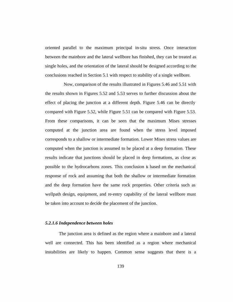
139

oriented parallel to the maximum principal in-situ stress. Once interaction

between the mainbore and the lateral wellbore has finished, they can be treated as

single holes, and the orientation of the lateral should be designed according to the

conclusions reached in Section 5.1 with respect to stability of a single wellbore.

Now, comparison of the results illustrated in Figures 5.46 and 5.51 with

the results shown in Figures 5.52 and 5.53 serves to further discussion about the

effect of placing the junction at a different depth. Figure 5.46 can be directly

compared with Figure 5.52, while Figure 5.51 can be compared with Figure 5.53.

From these comparisons, it can be seen that the maximum Mises stresses

computed at the junction area are found when the stress level imposed

corresponds to a shallow or intermediate formation. Lower Mises stress values are

computed when the junction is assumed to be placed at a deep formation. These

results indicate that junctions should be placed in deep formations, as close as

possible to the hydrocarbons zones. This conclusion is based on the mechanical

response of rock and assuming that both the shallow or intermediate formation

and the deep formation have the same rock properties. Other criteria such as

wellpath design, equipment, and re-entry capability of the lateral wellbore must

be taken into account to decide the placement of the junction.

5.2.1.6 Independence between holes

The junction area is defined as the region where a mainbore and a lateral

well are connected. This has been identified as a region where mechanical

instabilities are likely to happen. Common sense suggests that there is a

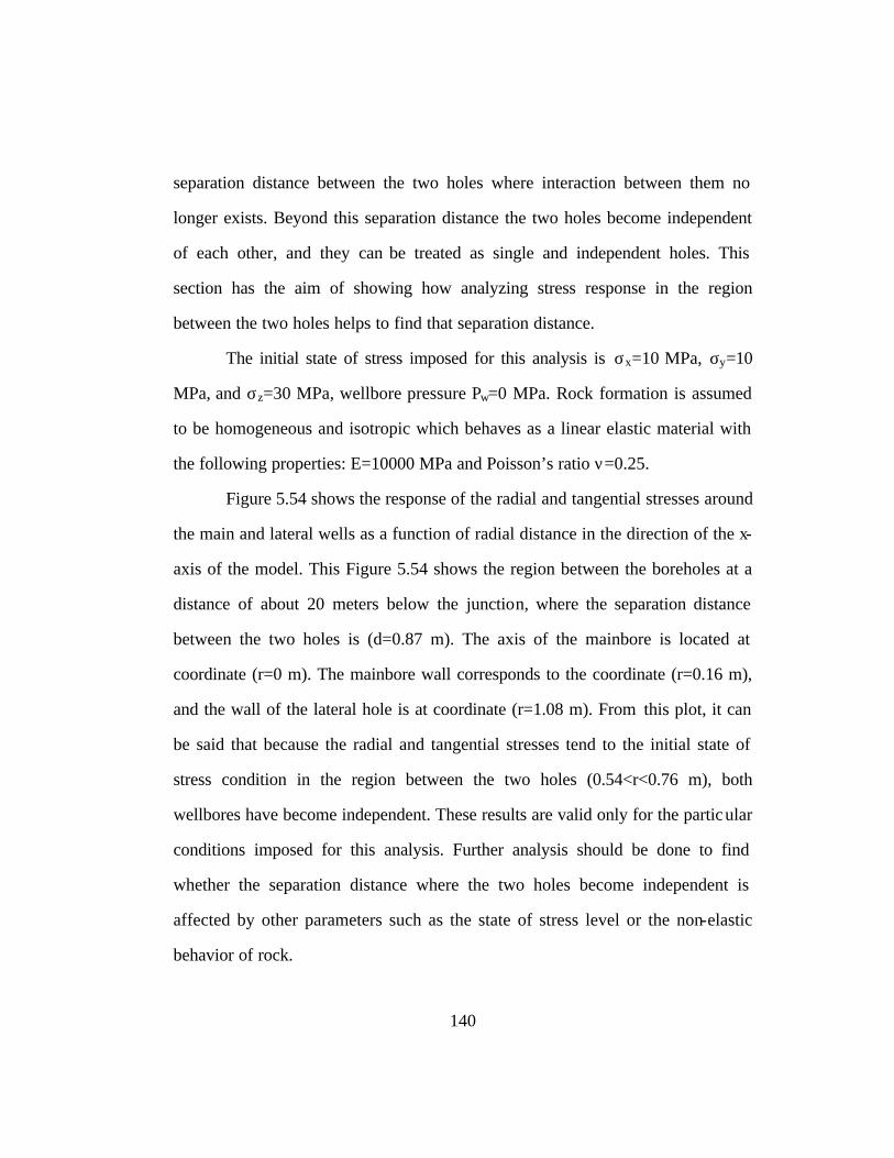
140

separation distance between the two holes where interaction between them no

longer exists. Beyond this separation distance the two holes become independent

of each other, and they can be treated as single and independent holes. This

section has the aim of showing how analyzing stress response in the region

between the two holes helps to find that separation distance.

The initial state of stress imposed for this analysis is σx=10 MPa, σy=10

MPa, and σz=30 MPa, wellbore pressure Pw=0 MPa. Rock formation is assumed

to be homogeneous and isotropic which behaves as a linear elastic material with

the following properties: E=10000 MPa and Poisson’s ratio ν=0.25.

Figure 5.54 shows the response of the radial and tangential stresses around

the main and lateral wells as a function of radial distance in the direction of the x-

axis of the model. This Figure 5.54 shows the region between the boreholes at a

distance of about 20 meters below the junction, where the separation distance

between the two holes is (d=0.87 m). The axis of the mainbore is located at

coordinate (r=0 m). The mainbore wall corresponds to the coordinate (r=0.16 m),

and the wall of the lateral hole is at coordinate (r=1.08 m). From this plot, it can

be said that because the radial and tangential stresses tend to the initial state of

stress condition in the region between the two holes (0.54<r<0.76 m), both

wellbores have become independent. These results are valid only for the particular

conditions imposed for this analysis. Further analysis should be done to find

whether the separation distance where the two holes become independent is

affected by other parameters such as the state of stress level or the non-elastic

behavior of rock.

141

5.2.1.7 Complex Multilateral Scenarios

Up to the knowledge of the author, no research has been conducted in

analyzing the effect of two lateral wellbores with the same starting point from the

mainbore on wellbore stability of the junction. Section 5.2.1.5 discussed the effect

of changing the placement of the junction from a shallow or intermediate

formation to a deep formation. That discussion is limited to consider the mainbore

is vertical with the lateral wellbore oriented in the direction of one of the principal

in-situ stresses. That analysis is applicable to a multilateral scenario where the

junction is placed somewhere above the hydrocarbons zone, in the overburden.

When reservoir management requires construction of a multilateral in a

single producing formation, a different analysis is required to study the stability of

the junction. The junction is assumed to be located into the producing formation

with the mainbore and the two laterals lying on the horizontal plane. This section

has the aim of providing a basic understanding about the effect of three wellbores

interacting on the stability of the junction when the junction is placed in a

producing formation.

Three elastic stress-displacement analyses are done at three different

orientations of the mainbore wellbore. The first is for the mainbore in the

direction of the maximum horizontal principal in-situ stress, azimuth equals zero

degrees (a=0o). The second is for the mainbore with an azimuth equals 45 degrees

(a=45o), and the third for the mainbore in the direction of the minimum horizontal

principal in-situ stress, azimuth equals ninety degrees (a=90o). The elastic

142

constants are the same as in Papanastasiou et al. (2002) study: E=22500 MPa and

ν=0.2. The stress level applied is the following σx=σH=30 MPa, σy=σh=18 MPa,

and σz=σv=50 MPa.

The results obtained are shown in contour plots of Mises stresses in

Figures 5.55 through 5.57. The first comment about these plots is that the region

that is prone to failure is in any case the junction. Secondly, comparison of these

figures confirms that drilling a horizontal well in the direction of the minimum

horizontal principal in-situ stress (a=90o) constitutes the most stable condition. It

can be seen in these figures that once the junction fails the next region to fail is

the mainbore. Red in these contour plots indicates zones that are more likely to

fail. It can be seen in Figure 5.55 (a=0o) a red zone in the mainbore, which

indicate failure in the mainbore while in Figure 5.57 (a=90o) the no presence of a

red zone indicates that the wellbores remain stable. The third important aspect

from these plots is that the stability of the junction is slightly affected by the

azimuth of the mainbore. Maximum Mises stresses are computed when the

mainbore is oriented with a=90. When a=0o, the maximum Mises stress is 1022

MPa. When a=45o, then the maximum Mises stress is 1042 MPa, and the

maximum Mises stress is1089 MPa when a=90o.

143

Table 5.1 Data from a drained triaxial test (from Atkinson and Bransby 1978).

Axial force (N)

Change of length (mm)

Volume of Water expelled (mm3x103

)

Volumetric strain

Axial strain (Fraction)

Area (m2x10-3)

q’ (Mpa)

0 0 0 0 0 1.134 0

115 -1.95 0.88 0.010 0.025 1.151 0.10

235 -5.85 3.72 0.042 0.075 1.174 0.20

325 -11.70 7.07 0.080 0.150 1.227 0.26

394 -19.11 8.40 0.095 0.245 1.359 0.29

458 -27.30 8.40 0.095 0.350 1.579 0.29

Table 5.2 Isotropic compression test results (from Atkinson and Bransby 1978).

Cell pressure (MPa)

Volume of water expelled (cm3)

Volume of the sample (cm3)

Specific volume

ln p’

0.020 0 88.5 2.74 -3.91

0.060 7.2 81.3 2.50 -2.81

0.200 15.0 73.5 2.28 -1.61

1.000 25.4 63.1 1.96 0

0.200 22.8 65.7 2.04 -1.61

0.060 20.8 67.7 2.08 -2.81

144

Table 5.3 Effect of varying M value on hole closure.

Model Case “A” Low stress level

Case “B” Intermediate stress level Hole closure (% of radius)

Case “C” High stress level

Elastic 0.121 0.310 0.431

Cam-Clay M=3.0 0.121 0.310 0.431

Cam-Clay M=2.0 0.121 0.310 0.544

Cam-Clay M=1.9 0.121 0.310 2.668

Cam-Clay M=1.8 0.121 0.310 *

Cam-Clay M=1.5 0.121 0.310 *

Cam-Clay M=1.2 0.125 0.310 *

Cam-Clay M=1.1 0.129 0.621 *

Cam-Clay M=1.09 0.129 1.329 *

Cam-Clay M=1.085 0.129 2.000 *

Cam-Clay M=0.9 0.148 * *

* Excessive deformation occurs so that the plasticity-algorithm used by Abaqus is unable to find a solution.

145

Table 5.4 Values of parameters for various clays (from Atkinson and Bransby 1978)

London clay Weald clay Kaolin

λs 0.161 0.093 0.260

κs 0.062 0.035 0.050

Γ 2.759 2.060 3.767

M 0.888 0.950 1.020

Table 5.5 Effect of varying λs and κs values on hole closure.

Model Hole closure (%)

Elastic 0.121

London clay 0.121

Weald clay 0.121

Kaolin 0.216

Table 5.6 Stress level imposed to analyze wellbore orientation

Case Depth σv σH σh *Pw

[ft] [MPa] [MPa] [MPa] [MPa] Shallow 2000 12 22.5 15 6 Intermediate 7000 48 60 40 21 Deep 18000 120 100 67 54

*Pw was calculated assuming water in the wellbore.

146

Table 5.7 Transversely isotropic rock properties used for sensitivity analysis.

Parameter Value Parameter Value

Exy 10000 MPa νxy 0.268

Exz 5000 MPa when (Rt=2) νxz 0.098

Exz 2000 MPa when (Rt=5) σx 100 MPa

Exz 1000 MPa when (Rt=10) σy 67 MPa

Gxz 3129 MPa when (Rt=2) σz 120 MPa

Gxz 1614 MPa when (Rt=5)

Gxz 893 MPa when (Rt=10)

Table 5.8 Orthotropic rock properties used for sensitivity analysis.

Parameter Value Parameter Value

Ex 10000 MPa νxy 0.268

Ez 5000 MPa νxz = νyz 0.098

Ey 6667 MPa when (Rp=1.5) CASE I σx 100 MPa

Ey 5000 MPa when (Rp=2) CASE II σy 67 MPa

σz 120 MPa

Gyz 3036 MPa when (Rp=1.5) Gxy 3943 MPa

Gyz 2277 MPa when (Rp=2) Gyz 2277 MPa

147

Table 5.9 Effect of rate of penetration on hole closure.

Rate of penetration [m/hr] Hole closure [%] Difference respect to one-step simulation (elastic) [%]

1 0.667 5.87

10 0.656 4.12

20 0.645 2.38

One-step (Elastic) 0.630 0.0

Table 5.10 Material properties for a coupled stress-diffusion analysis (from Chen et al. 2000).

Properties Units Model

Density of the sample Kg/m3 2278

Bulk modulus sample Gpa 18.87

Shear modulus sample Gpa 7.72

Friction angle sample Degrees 37

Cohesion sample MPa 6.3

Dilation angle sample Degrees 0

Tensile strength sample MPa 2.07

Porosity sample % 24.23

Mobility ratio sample (m/s)/(Pa/m) 5.14E-20

Bulk modulus fluid GPa 2.0

Density fluid Kg/m3 1000

148

0.02.04.06.08.0

10.012.014.016.018.020.0

0 0.25 0.5 0.75 1 1.25Radius (m)

Str

ess

(MP

a)

Radial Tangential

Corresponding to the Wellbore wall

Figure 5.1 Stress distribution around a wellbore: Elastic case.

8.0

10.0

12.0

14.0

16.0

18.0

20.0

0 0.1 0.2 0.3 0.4 0.5 0.6 0.7Radius (m)

Str

ess

(MP

a)

Elastic Cam-Clay

Corresponding to thewellbore wall

Relaxation of thetangential stress

Extent of the plastic zone

Figure 5.2 Comparison of tangential stresses

149

Figure 5.3 Contour plot showing the extent of the plastic zone.

150

8.0

10.0

12.0

14.0

16.0

18.0

20.0

0 0.25 0.5 0.75 1 1.25Radius (m)

Str

ess

(MP

a)

Elastic Cam-Clay D-PragerCorresponding to thewellbore wall

Maximum tangential stress valueslocated inside the formation

Figure 5.4 Comparison between tangential stress solutions.

0.0

2.0

4.0

6.0

8.0

10.0

12.0

0 0.25 0.5 0.75 1 1.25Radius (m)

Str

ess

(MP

a)

Elastic Cam-Clay D-PragerCorresponing to thewellbore wall

Figure 5.5 Comparison between radial stress solutions.

151

Figure 5.6 Analysis of compressive failure for the elements in the immediate vicinity of the wellbore.

0

2

4

6

8

10

12

14

16

18

20

0 2 4 6 8Effective mean stress [MPa]

Effe

ctiv

e M

ises

stre

ss [M

Pa]

Elastic Cam-Clay D-Prager Envelope Initial State

Failure Envelope

Elastic

Cam-ClayDrucker-Prager

Initial state

Region

ABC

152

8.0

10.0

12.0

14.0

16.0

18.0

20.0

0 0.25 0.5 0.75 1 1.25

Radius (m)

Tan

gent

ial s

tres

s (M

Pa)

M=1.5 M=1.1 M=1.0 M=0.9


Figure 5.7 Effect of M variation on the tangential stress response: Cam-Clay

8.0

10.0

12.0

14.0

16.0

18.0

20.0

0 0.25 0.5 0.75 1 1.25

Radius (m)

Str

ess

(MP

a)

Kaolin London clay Weald clay


Difference between the extent of the plastic zones

Figure 5.8 Tangential stress behavior

153

Figure 5.9 Representation of the principal in-situ stresses in a shallow formation in a tectonically active stressed region (σH>σh>σv).

Global coordinate system

σσvv==1122 MMPPaa

σhh=15 MPa

σσHH==2222..55 MMPPaa

yy’’

zz’’

xx’’

154

a) azimuth=0

0

10

20

30

40

50

0 15 30 45 60 75 90

Inclination [degrees]

Str

esse

s [M

Pa]

Misses Mean

b) azimuth=45

0

10

20

30

40

50

0 15 30 45 60 75 90


Str

esse

s [M

Pa]

Misses Mean

c) azimuth=90

0

10

20

30

40

50

0 15 30 45 60 75 90


Str

esse

s [M

Pa]

Misses Mean

Figure 5.10 Maximum Mises and Mean stresses vs hole deviation for three different azimuth values in a shallow formation (elastic rock).

155

0

10

20

30

40

50

0 5 10 15 20 25 30

Mean [MPa]

Mis

es [M

Pa]

a=0 a=45 a=90

Figure 5.11 Effect of varying angle deviation on the maximum p’ and q’ values in a shallow formation (elastic rock).

0.00.10.20.30.40.50.60.70.80.91.0

0 15 30 45 60 75 90


Hol

e cl

osur

e [%

]

a=0 a=45 a=90

Figure 5.12 Maximum hole closure vs wellbore inclination in a shallow formation (elastic rock).

0o 90o

90o

90o 60o

Failure envelope

156


Figure 5.13 Representation of the principal in-situ stresses in an intermediate formation in a tectonically active stressed region (σH>σv>σh).

σσvv==4488 MMPPaa

σhh=40 MPa

σσHH==6600 MMPPaa

yy’’

zz’’

xx’’

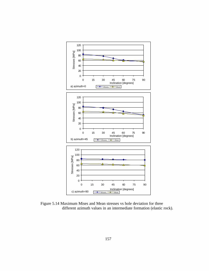
157

a) azimuth=0

0

20

40

60

80

100

120

0 15 30 45 60 75 90Inclination [degrees]

Str

esse

s [M

Pa]

Misses Mean

b) azimuth=45

0

20

40

60

80

100

120


Str

esse

s [M

Pa]

Misses Mean

c) azimuth=90

0

20

40

60

80

100

120

0 15 30 45 60 75 90


Str

esse

s [M

Pa]

Misses Mean

Figure 5.14 Maximum Mises and Mean stresses vs hole deviation for three different azimuth values in an intermediate formation (elastic rock).

158

30

40

50

60

70

80

90

30 40 50 60 70

Mean effective [MPa]

Mis

es e

ffect

ive

[MP

a]

a=0 a=45 a=90

Figure 5.15 Effect of varying angle deviation on the maximum Mean and Mises effective stresses in an intermediate formation (elastic rock).

0.0

0.1

0.20.3

0.4

0.50.6

0.7

0.8

0.91.0

0 15 30 45 60 75 90


Hol

e cl

osur

e [%

]

a=0 a=45 a=90

Figure 5.16 Maximum hole closure vs wellbore inclination in an intermediate formation (elastic rock).

0o

90o

90o 90o

Failure envelope

159


Figure 5.17 Representation of the principal in-situ stresses in a deep formation in a tectonically active stressed region (σv>σH>σh).

σσvv==112200 MMPPaa

σhh=67 MPa

σσHH==110000 MMPPaa

yy’’

zz’’

xx’’

160

a) azimuth=0

020406080

100120140160180200

0 15 30 45 60 75 90


Str

esse

s [M

Pa]

Misses Mean

b) azimuth=45

020406080

100120140160180200

0 15 30 45 60 75 90


Str

esse

s [M

Pa]

Misses Mean

c) azimuth=90

020406080

100120140160180200

0 15 30 45 60 75 90


Str

esse

s [M

Pa]

Misses Mean

Figure 5.18 Maximum Mises and Mean stresses vs hole deviation for three different azimuth values in a deep formation (elastic rock).

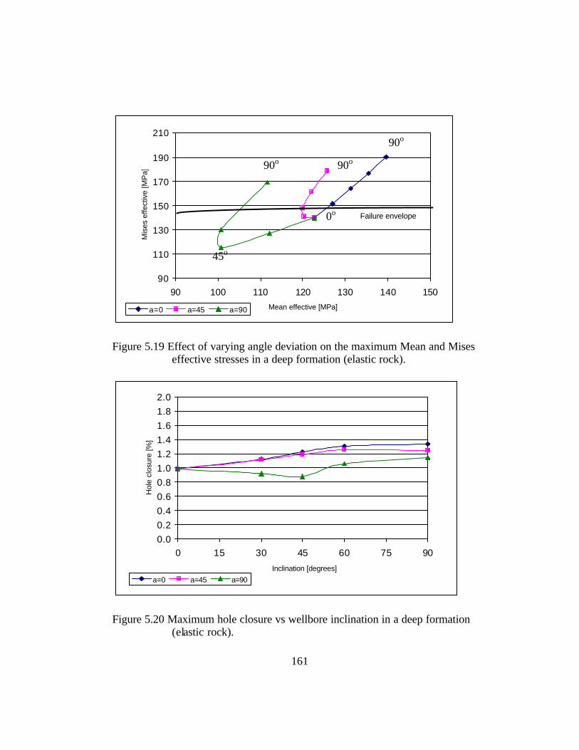
161

90

110

130

150

170

190

210

90 100 110 120 130 140 150


Mis

es e

ffect

ive

[MP

a]

a=0 a=45 a=90

Figure 5.19 Effect of varying angle deviation on the maximum Mean and Mises effective stresses in a deep formation (elastic rock).

0.00.20.40.60.81.01.21.41.61.82.0

0 15 30 45 60 75 90


Hol

e cl

osur

e [%

]

a=0 a=45 a=90

Figure 5.20 Maximum hole closure vs wellbore inclination in a deep formation (elastic rock).

0o

45o

90o

90o

90o

Failure envelope

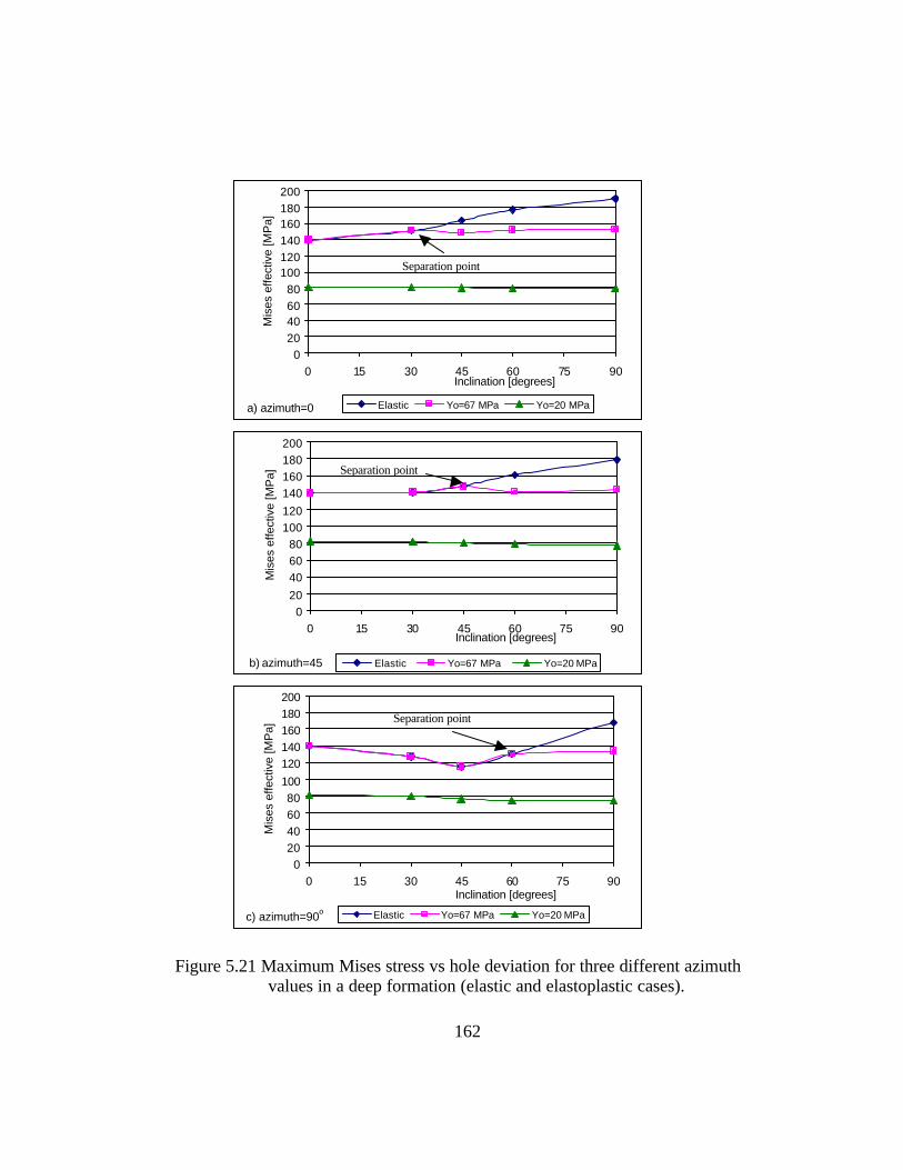
162

a) azimuth=0

020406080

100120140160180200


Mis

es e

ffect

ive

[MP

a]

Elastic Yo=67 MPa Yo=20 MPa

b) azimuth=45

020

406080

100120

140160180200


Mis

es e

ffect

ive

[MP

a]


c) azimuth=90o

020406080

100

120140160180200


Mis

es e

ffect

ive

[MP

a]


Figure 5.21 Maximum Mises stress vs hole deviation for three different azimuth values in a deep formation (elastic and elastoplastic cases).

Separation point

Separation point

Separation point

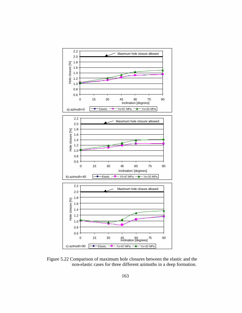
163

a) azimuth=0

0.6

0.8

1.0

1.2

1.4

1.6

1.8

2.0

2.2


Hol

e cl

osur

e [%

]


Maximum hole closure allowed

b) azimuth=45

0.6

0.8

1.0

1.2

1.4

1.6

1.8

2.0

2.2


Hol

e cl

osur

e [%

]

Elastic Y0=67 MPa Yo=20 MPa


c) azimuth=90

0.6

0.8

1.0

1.2

1.4

1.6

1.8

2.0

2.2


Hol

e cl

osur

e [%

]



Figure 5.22 Comparison of maximum hole closures between the elastic and the non-elastic cases for three different azimuths in a deep formation.

164

a) azimuth=0

0

50

100

150

200

70 90 110 130 150Mean effective [MPa]

Mis

es e

ffect

ive

[MP

a]


b) azimuth=45

0

50

100

150

200

70 90 110 130 150Mean effective [degrees]

Mis

es e

ffect

ive

[MP

a]

Elastic Y0=67 MPa Yo=20 MPa

c) azimuth=90

0

50

100

150

200

70 90 110 130 150Mean effective [degrees]

Mis

es e

ffect

ive

[MP

a]


Figure 5.23 Effect of varying inclination angle on the maximum Mises and Mean effective stresses. Deep formation (elastic and elastoplastic cases).

0o 90o

90o

0o 90o

Failure envelope

Failure envelope

90o

90o

0o

0o

45o

30o

Failure envelope

60o

90o

90o

0o

0o

165

a) azimuth=0

100

120

140

160

180

200

0 15 30 45 60 75 90


Mis

es e

ffect

ive[

MP

a]

Rt=1 Rt=2 Rt=5 Rt=10

b) azimuth=45

100

120

140

160

180

200

0 15 30 45 60 75 90


Mis

es e

ffect

ive

[MP

a]


c) azimuth=90

100110120130140150160170180190200

0 15 30 45 60 75 90


Mis

es e

ffect

ive

[MP

a]


Figure 5.24 Maximum Mises stresses vs hole deviation at three different Rt values in a deep transversely isotropic formation (elastic rock).

166

a) azimuth=0

100

125

150

175

200

100 110 120 130 140 150


Mis

es e

ffect

ive

[MP

a]


0o

90o90o

0o

b) azimuth=45

100

125

150

175

200

90 100 110 120 130 140 150


Mis

es e

ffect

ive

[MP

a]


0o

90o90o

0o

c) azimuth=90

100

125

150

175

200

90 100 110 120 130 140 150


Mis

es e

ffect

ive

[MP

a]


0o

90o

90o

0o

Figure 5.25 Comparison of the maximum p’ and q’ values when varying the deviation angle. Different Rt . Transversely isotropic formation.

Failure envelope

Failure envelope

Failure envelope

167

a) azimuth=0

0.6

0.8

1.0

1.2

1.4

1.6

1.8

2.0

0 15 30 45 60 75 90


Hol

e cl

osur

e [%

]


b) azimuth=45

0.6

0.8

1.0

1.2

1.4

1.6

1.8

2.0

0 15 30 45 60 75 90


Hol

e cl

osur

e [%

]


c) azimuth=90

0.6

0.8

1.0

1.2

1.4

1.6

1.8

2.0


Hol

e cl

osur

e [%

]


Figure 5.26 Maximum hole closure vs wellbore inclination. Different Rt. Transversely isotropic formation.

168

a) azimuth=0

100

120

140

160

180

200

220

0 15 30 45 60 75 90


Mis

es e

ffect

ive

[MP

a]

Rt=2 Rp=1.5 Rp=2

b) azimuth=45

100

120

140

160

180

200

220

0 15 30 45 60 75 90


Mis

es e

ffect

ive

[MP

a]

Rt=2 Rp=1.5 Rp=2

c) azimuth=90

100

120

140

160

180

200

220

0 15 30 45 60 75 90


Mis

es e

ffect

ive

[MP

a]

Rt=2 Rp=1.5 Rp=2

Figure 5.27 Maximum Mises stresses vs hole deviation at three different Rp values in a deep orthotropic formation (elastic rock).

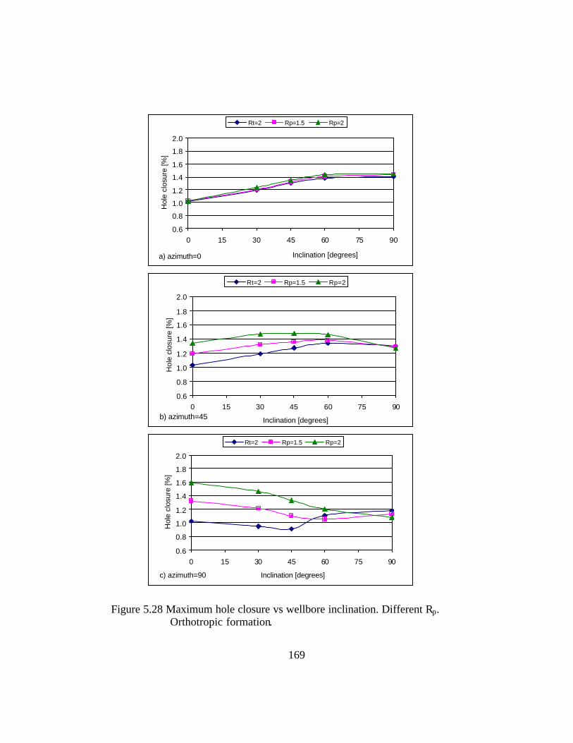
169

a) azimuth=0

0.6

0.8

1.0

1.2

1.4

1.6

1.8

2.0

0 15 30 45 60 75 90


Hol

e cl

osur

e [%

]

Rt=2 Rp=1.5 Rp=2

b) azimuth=45

0.6

0.8

1.0

1.2

1.4

1.6

1.8

2.0

0 15 30 45 60 75 90


Hol

e cl

osur

e [%

]

Rt=2 Rp=1.5 Rp=2

c) azimuth=90

0.6

0.8

1.0

1.2

1.4

1.6

1.8

2.0

0 15 30 45 60 75 90


Hol

e cl

osur

e [%

]

Rt=2 Rp=1.5 Rp=2

Figure 5.28 Maximum hole closure vs wellbore inclination. Different Rp. Orthotropic formation.

170

Figure 5.29 Rate of deformation influence on the uniaxial stress-strain curves and failure of sandstone (from Cristescu and Hunsche 1998).

171

3000.00

3000.05

3000.10

3000.15

3000.20

3000.25

3000.30

3000.35

3000.40

3000.45

3000.500.0 0.1 0.2 0.3 0.4 0.5 0.6 0.7 0.8 0.9 1.0

Hole closure (%)

Figure 5.30 Comparison of hole closure between one-step and multi-step analysis.

3000.00

3000.05

3000.10

3000.15

3000.20

3000.25

3000.30

3000.35

3000.40

3000.45

3000.500.0 0.2 0.4 0.6 0.8 1.0

Hole closure (%)

Dep

th [m

]

t=6 t=12 t=18 t=24 t=30

Figure 5.31 Progress of drilling with time showing the hole closure behind the advancing face of the wellbore.

One-step

Multi-step

Advancing face of the wellbore at corresponding times

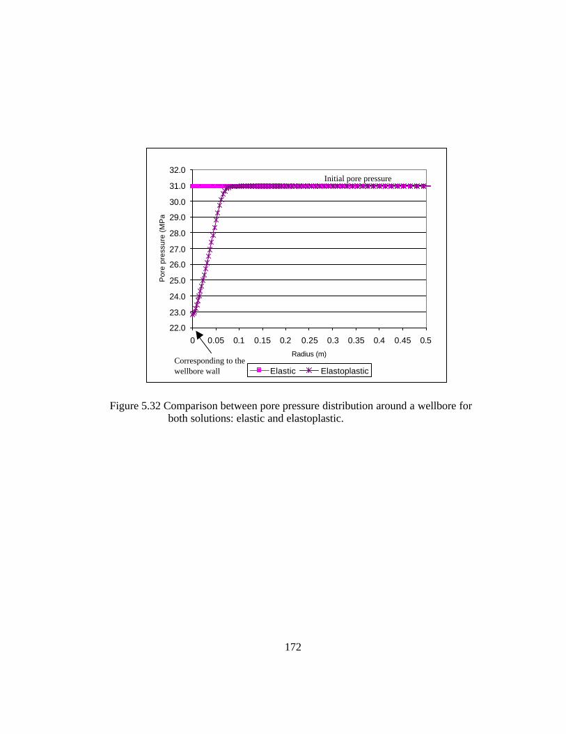
172

22.0

23.0

24.0

25.0

26.0

27.0

28.0

29.0

30.0

31.0

32.0

0 0.05 0.1 0.15 0.2 0.25 0.3 0.35 0.4 0.45 0.5

Radius (m)

Por

e pr

essu

re (

MP

a)

Elastic Elastoplastic

Figure 5.32 Comparison between pore pressure distribution around a wellbore for both solutions: elastic and elastoplastic.

Corresponding to the wellbore wall

Initial pore pressure

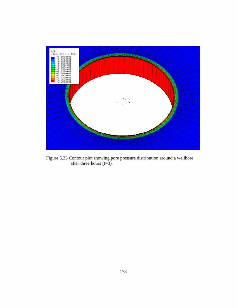
173

Figure 5.33 Contour plot showing pore pressure distribution around a wellbore after three hours (t=3).

174

22.0

23.0

24.0

25.0

26.0

27.0

28.0

29.0

30.0

31.0

32.0

0 0.05 0.1 0.15 0.2 0.25 0.3 0.35 0.4 0.45 0.5

Radius (m)

Por

e pr

essu

re(M

Pa)

t=3 hr t=27 hr

Figure 5.34 Pore pressure distribution as a function of time and radial distance from the wellbore wall.

22.0

23.0

24.0

25.0

26.0

27.0

28.0

29.0

30.0

31.0

32.0

0 0.05 0.1 0.15 0.2 0.25 0.3 0.35 0.4 0.45 0.5

Radius (m)

Por

e pr

essu

re (

MP

a)

Ki=5.14E-20 Ki=5.14E-18 Ki=5.14E-17

Figure 5.35 Pore pressure distribution as a function of radial distance from the wellbore wall for different permeability conditions.



175

18.019.020.021.022.023.024.025.026.027.028.029.030.031.032.0

0 0.05 0.1 0.15 0.2 0.25 0.3 0.35 0.4 0.45 0.5Radius (m)

Por

e pr

essu

re (

MP

a)

Yo=45 MPa Yo=55 Mpa Yo=68 MPa Elastic

Figure 5.36 Effect of yield stress variation on the response of pore pressure distribution around a wellbore.

22.0

23.0

24.0

25.0

26.0

27.0

28.0

29.0

30.0

31.0

32.0

0 0.05 0.1 0.15 0.2 0.25 0.3 0.35 0.4 0.45 0.5

Radius (m)

Por

e pr

essu

re(M

Pa)

cf=0 cf=4.79E-4 cf=1.0E-3 Cf=1.89E-2

Figure 5.37 Effect of fluid compressibility variation on the response of pore pressure distribution around a wellbore.



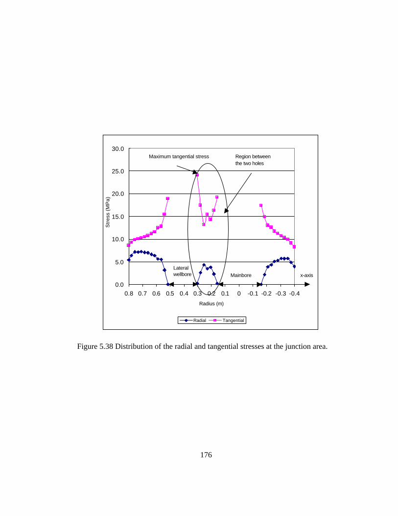
176

0.0

5.0

10.0

15.0

20.0

25.0

30.0

-0.4-0.3-0.2-0.100.10.20.30.40.50.60.70.8

Radius (m)

Str

ess

(MP

a)

Radial Tangential

x-axisMainboreLateralwellbore

Maximum tangential stress Region betweenthe two holes

Figure 5.38 Distribution of the radial and tangential stresses at the junction area.

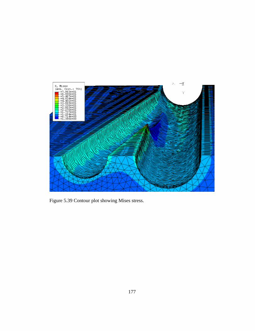
177

Figure 5.39 Contour plot showing Mises stress.

178

Figure 5.40 Contour plot showing displacement in the x-direction.

Closure Enlargement

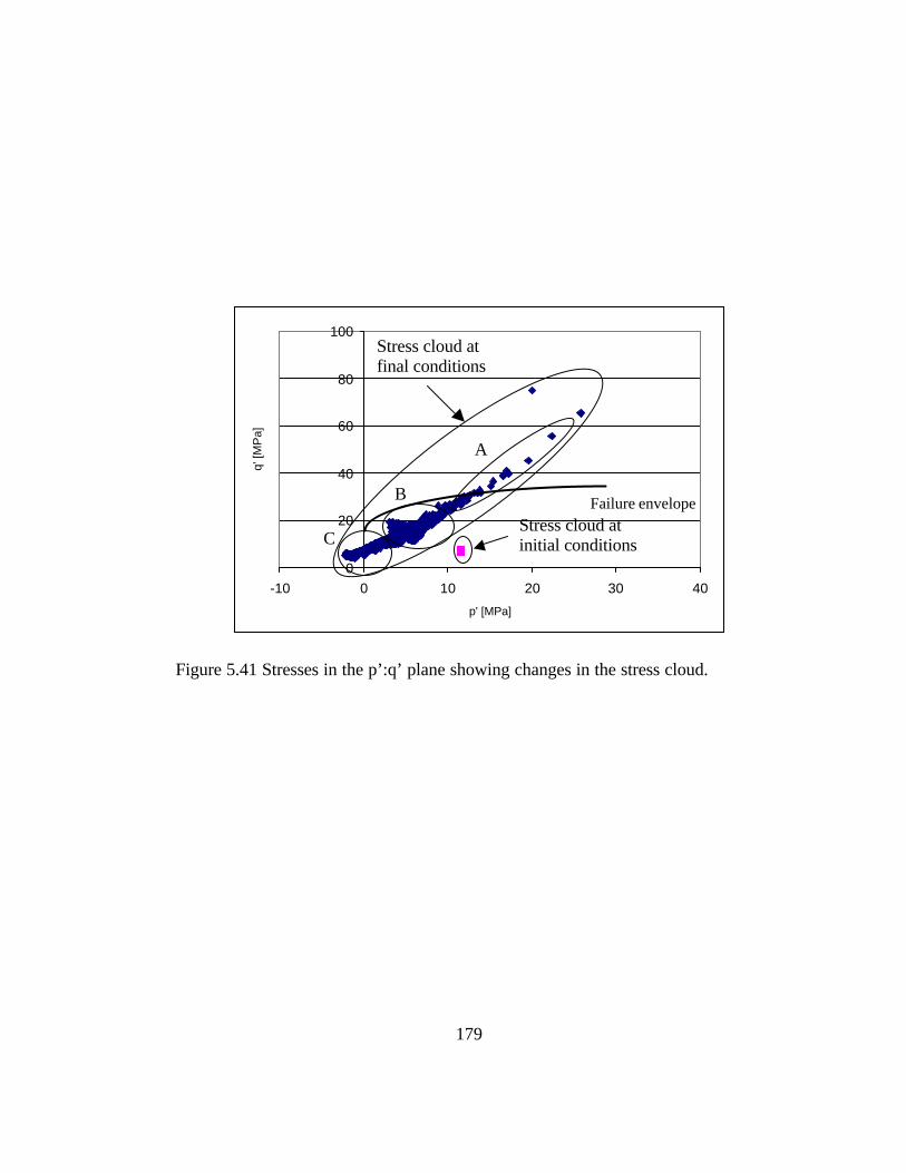
179

0

20

40

60

80

100

-10 0 10 20 30 40

p' [MPa]

q' [M

Pa]

Figure 5.41 Stresses in the p’:q’ plane showing changes in the stress cloud.

Failure envelope Stress cloud at initial conditions

A

B

C

Stress cloud at final conditions

180

Figure 5.42 3-D representation showing the three regions A, B, and C identified at the junction area.

B

C

A

181

2.5 o Junction angle

0

20

40

60

80

100

-10 -5 0 5 10 15 20 25 30 35 40

p' [MPa]

q' [M

Pa]

b) 5o Junction angle

0

20

40

60

80

100

-10 -5 0 5 10 15 20 25 30 35 40

p' [MPa]

q' [M

Pa]

c) 10o Junction angle

0

20

40

60

80

100

-10 -5 0 5 10 15 20 25 30 35 40

p' [MPa]

q' [M

Pa]

Figure 5.43 Effect of variation of the junction angle on the stress cloud.

Failure envelope

Failure envelope

Failure envelope

182

a) 10.625 in. diameter lateral hole

0

20

40

60

80

100

120

140

160

-10 0 10 20 30 40 50 60p' [MPa]

q' [M

Pa]

b) 6.75 in. diameter lateral hole

0

20

40

60

80

100

120

140

160

-10 0 10 20 30 40 50 60

p' [MPa]

q' [M

Pa]

Figure 5.44 Effect of variation of the diameter of the lateral well on the stress cloud.

Failure envelope

Failure envelope

183

Figure 5.45 Contour plot of displacements when the lateral is oriented with an azimuth (a=90o).

184

Figure 5.46 Contour plot of Mises stresses when the lateral is oriented with an azimuth (a=90o).

Failure in the junction

185

Figure 5.47 Contour plot of Mises stresses showing failure in the lateral wellbore at a higher stress level.

The lateral wellbore fails after the junction fails

186

Figure 5.48 Contour plot of Mises stresses showing that the most likely region to fail after the junction when the lateral is oriented with an azimuth (a=0o) is the mainbore.

The mainbore fails after the junction fails

187

Figure 5.49 Contour plot of Mises stresses showing breakout orientation when the lateral is oriented with an azimuth (a=90o).

Breakout orientation

188

Figure 5.50 Contour plot of Mises stresses showing breakout orientation when the lateral is oriented with an azimuth (a=0o).

Breakout orientation

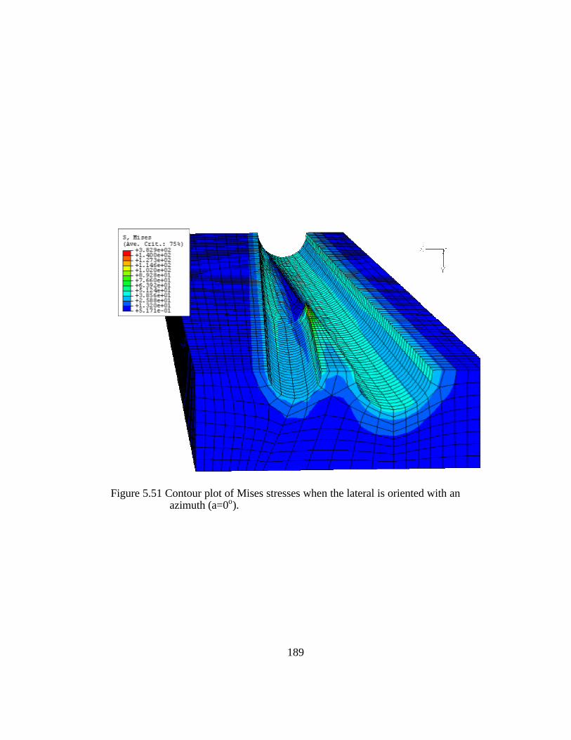
189

Figure 5.51 Contour plot of Mises stresses when the lateral is oriented with an azimuth (a=0o).

190

Figure 5.52 Contour plot of Mises stresses when the lateral is oriented with an azimuth (a=0o) and in a deep formation.

191

Figure 5.53 Contour plot of Mises stresses when the lateral is oriented with an azimuth (a=90o) and in a deep formation.

192

0

5

10

15

20

25

0 0.1 0.2 0.3 0.4 0.5 0.6 0.7 0.8 0.9 1 1.1 1.2

Radius (m)

Str

ess

(Pa)

Radial Tangential

x-axis

Lateral wallMainborewall

Mainboreaxis

Region where radial and tangental stressestend to the initial state of stress

Figure 5.54 Stress distribution in the region between the two boreholes showing independence between them.

193

Figure 5.55 Contour plot of Mises stresses of a horizontal mainbore with two laterals when the mainbore is oriented with an azimuth (a=0o).

Failure in the mainbore

194


Failure in the mainbore

195


196

Chapter 6: Conclusions and Recommendations

The following conclusions and recommendations were reached from this

study of the stability of single wellbores and multilateral junctions. These

conclusions and recommendations are given with the aim to contribute to

subsequent investigation on this topic.

The analysis of the stability of a single wellbore led to the following

conclusions.

1) The three-dimensional finite element model used for computations of

strains and stresses around a single wellbore in this study is reliable for

the analysis of the stability of a wellbore oriented in any direction.

2) When rock is characterized using a constitutive model that takes into

account the non-elastic behavior of the rock, such as the Cambridge or

the Drucker-Prager models applied in this work, a substantial

relaxation of the tangential stress is observed in the region near the

wellbore. This relaxation zone is attributed to high effective stress

concentration, which causes the plastic response of the rock in this

region. Comparison of the results obtained with the elastic constitutive

model and the two non-elastic constitutive models demonstrated that

relaxation of the tangential stress in the region near the wellbore

increases stability regarding collapse.

3) Comparing the results obtained from the elastic constitutive model and

the two non-elastic constitutive models, it was concluded that

197

analyzing wellbore stability for collapse using a peak-strength criterion

is pessimistic when the rock exhibits non-elastic behavior. In this case,

a yield criterion should be taken into account.

4) The analysis of the effect of varying wellbore inclination and azimuth

on the stability of an oriented wellbore showed the best orientations

for a single wellbore to be drilled at different depths. In a shallow or

intermediate formation, stability regarding collapse is improved by

inclining the wellbore in the direction parallel to the maximum

horizontal stress (σH). In a deep formation, wellbore trajectories close

to the vertical should be pursued. When this is not possible, the least

adverse wellbore stability condition is drilling the wellbore in the

direction parallel to the minimum horizontal stress (σh) with

inclination angles less than 45o.

5) The best orientation to drill a horizontal wellbore regarding stability is

in the direction parallel to the minimum horizontal stress (σh).

6) In general, hole closure of a deviated wellbore and Mises stresses

around this wellbore slightly increase when the degree of anisotropy of

a given formation increases. The stability of the wellbore decreases

when the wellbore is oriented towards the direction parallel to the

maximum horizontal stress (σH). Thus, a deviated wellbore drilled into

an anisotropic formation is slightly more unstable than one drilled into

an isotropic formation.

198

7) When analyzing the transient phenomenon associated with the effect

of rate of deformation of rocks, the only mode that accounts correctly

for the non-elastic behavior of a formation associated with its rate of

deformation is a three-dimensional model in conjunction with

simulation of drilling in a muti-step process. This transient

phenomenon cannot be quantified when rock is characterized with the

elasticity theory.

The second part of the conclusions was reached from the analysis of the

stability of a junction in a multilateral scena rio.

1) Because the results obtained using the axis-symmetric three-

dimensional finite element models for the study of wellbore stability in

multilateral junctions were in reasonable agreement with recent

published results from experimental tests, these models can be trusted

to perform efficient stability analysis in multilateral scenarios.

2) Three main regions were identified in the junction area. Two of these

regions were defined as critical regarding failure and the third as

stable. A collapse region was located between the mainbore and the

lateral wellbores, and a fracture region was located in the window

created by drilling the lateral wellbore.

199

3) Maximum stress values are located in the region between both holes.

These maximum stress values indicate that the onset of collapse failure

is in the junction.

4) Limited benefits should be expected in regards to wellbore stability at

the junction area when the angle between the mainbore and the lateral

wellbore is increased. The same conclusion applies with respect to

wellbore stability when the diameter of the lateral wellbore is

increased.

5) Based on the mechanical response of rock, junctions of multilateral

wells should be placed as close as possible to the hydrocarbon zones.

Other criteria such as wellpath design, equipment, and re-entry

capability of the lateral wellbore should be taken into account to

decide the optimum placement of the junction.

6) The most stable junction, independently of the depth of its placement,

is with the lateral wellbore axis oriented parallel to the maximum

principal in-situ stress (σH). Once interaction between the mainbore

and the lateral wellbore has finished, both wellbores should be treated

as single holes, and the orientation of the lateral should be designed

according to the conclusions reached with respect to stability of a

single wellbore.

7) Analysis of the behavior of the tangential and radial stresses in the

region between the mainbore and the lateral wellbore serves to define

200

the distance below the junction where the two holes become

independent.

8) When a junction is located in a homogeneous and isotropic producing

formation with the mainbore and the two laterals lying in the

horizontal plane, stress analysis indicates that the onset of collapse

failure is in the junction. Once the junction fails, the next region prone

to fail is the mainbore.

9) In the same scenario of a junction located in a homogeneous and

isotropic producing formation with the mainbore and the two laterals

lying on the horizontal plane, it was found that the stability of the

junction is slightly affected by the azimuth of the mainbore.

10) When increasing wellbore pressure, a fracture may be initiated in the

region of the window created by drilling the lateral wellbore. This

situation can lead to circulation losses of drilling or completion fluids.

In contrast, reduction of wellbore pressure can cause wellbore collapse

in the region between the holes.

11) Using ABAQUS commercial software based on finite element theory

constitutes a fundamental tool to design multilateral wells in regards to

parameters of design such as geometry, placement, and orientation of

the junction. ABAQUS is equipped to handle the sources of non-

linearity affecting the strain and stress responses of rock.

201

The results found in this study with respect to stability of single wellbores

and junctions in multilateral scenarios are the basis for recommending further

study of wellbore stability in the following topics.

1) The study of stability in multilateral junctions in this work was

restricted to the completion levels 1 defined in Chapter 1, where

mechanical support or hydraulic isolation at the junction are not

provided. This research was focused on the study of rock behavior.

Future work should include more complex scenarios found in

completion and production operations where casing and cement

modify the strength of the junction.

2) Further investigation is recommended about the effect of chemical

interaction between the drilling or completion fluids and the in-situ

formation fluids on the stability of the junction.

3) The results obtained in this study with regards to rock anisotropy were

limited to the effects that laminated sedimentary rocks cause on

wellbore stability when the bedding planes are horizontal. Further

analysis is recommended about the effect of varying the dip angle of

the bedding plane on wellbore stability of deviated wellbores.

4) Additional study is recommended regarding factors affecting

separation distance such as the in-situ state of stress and rock

properties.

202

5) Data on the in-situ state of stress are not the only important parameters

to be known, but also other parameters such as pore pressure and

reliable geomechanical characterization of rock and the fluids

contained in it. Further study is recommended on tools, techniques,

and laboratory tests that allow accurate characterization of rock, fluids,

and the in-situ stresses. In particular, it was shown that critical state

models such as the Cambridge model account for unconsolidated

sands and shales. The Cambridge model should be selected to analyze

shale behavior.

The set of conclusions here presented provide a real insight of rock

behavior regarding stability during the drilling of a single wellbore and the

junction in a multilateral scenario. These conclusions were the basis to propose

strategies to optimize drilling and completion design of single and multilateral

wells. Both conclusions and recommendations accomplish the primary objectives

stated in this research.

203

Appendix

ABAQUS Input File

A typical input file used in ABAQUS is shown. This contains the

sequence of instructions, data, and loading history representing a model. The

input file is divided in two main parts: the model data and the loading history.

Each part is composed of a number of blocks that contain the instructions and

data. The first part is called model data and contains all the information required

to define the structure to be analyzed and definition of material properties. The

second part defines the sequence of events in the simulation and is called loading

history. The loading history contains the loads and constrains and is subdivided

into a sequence of steps, each step defining a different stage of the simulation.

204

*********************************************************************** ********** TYPICAL ABAQUS INPUT FILE ********** *********************************************************************** *HEADING *PREPRINT, CONTACT=NO, ECHO=NO, MODEL=NO, HISTORY=NO *********************************************************************** ********** MODEL DATA ********** *********************************************************************** ** ********** NODAL COORDINATES ********** ** *NODE 56001, 0.0, -1.25, 0. 56033, 1.25, -1.25, 0. 56097, 1.25, 1.25, 0. 56161, -1.25, 1.25, 0. 56225, -1.25, -1.25, 0. 56257, 0.0, -1.25, 0. *NGEN 56001, 56033, 1 56033, 56097, 1 56097, 56161, 1 56161, 56225, 1 56225, 56257, 1 *NODE, SYSTEM=C 1, 0.1, -90., 0. 256, 0.1, -91.40625, 0. *NGEN, LINE=C, NSET=HOLE 1, 256, 1, , 0., 0., 0., 0., 0., 1. *NSET, NSET=GEN1, GENERATE 56001, 56256, 1 *NFILL, BIAS=.975 HOLE, GEN1, 112, 500 *NSET, NSET=ALLN, GENERATE 1, 56257 *NCOPY, SHIFT, CHANGE NUMBER=100000, OLD SET=ALLN 0., 0., 0.025 0., 0., 0., 0., 0., 1., 0. *NCOPY, SHIFT, CHANGE NUMBER=200000, OLD SET=ALLN 0., 0., 0.05 0., 0., 0., 0., 0., 1., 0. ** ********** ADDITIONAL NODE SETS ********** ** *NSET, NSET=WALL, GENERATE 1, 257, 2 100001, 100257, 4

205

200001, 200257, 2 *NSET, NSET=LEFT, GENERATE 56161, 56225, 2 156161, 156225, 4 256161, 256225, 2 *NSET, NSET=RIGHT, GENERATE 56033, 56097, 2 156033, 156097, 4 256033, 256097, 2 *NSET, NSET=BACK, GENERATE 56097, 56161, 2 156097, 156161, 4 256097, 256161, 2 *NSET, NSET=FRONT1, GENERATE 56001, 56033, 2 156001, 156033, 4 256001, 256033, 2 *NSET, NSET=FRONT2, GENERATE 56225, 56257, 2 156225, 156257, 4 256225, 256257, 2 *NSET, NSET=FRONT FRONT1, FRONT2 *NSET, NSET=TOP, GENERATE 1, 257, 2 1001, 1257, 4 2001, 2257, 2 3001, 3257, 4 4001, 4257, 2 5001, 5257, 4 6001, 6257, 2 7001, 7257, 4 8001, 8257, 2 9001, 9257, 4 10001, 10257, 2 *NSET, NSET=BOTTOM, GENERATE 200001, 200257, 2 201001, 201257, 4 202001, 202257, 2 203001, 203257, 4 204001, 204257, 2 205001, 205257, 4 206001, 206257, 2 207001, 207257, 4 208001, 208257, 2 209001, 209257, 4 210001, 210257, 2

206

** ********** ELEMENT CONNECTIVITY ********** ** *ELEMENT, TYPE=C3D20R, ELSET=HOLEIN 1, 1,2001,2005,5, 200001,202001,202005,200005, 1001,2003,1005,3, 201001,202003,201005,200003, 100001,102001,102005,100005 64, 253,2253,2001,1, 200253,202253,202001,200001, 1253,2255,1001,255, 201253,202255,201001,200255, 100253,102253,102001,100001 *ELGEN, ELSET=HOLE 1, 63, 4, 1, 28,2000,100 *ELGEN, ELSET=HOLE 64, 28, 2000, 100 *ELSET, ELSET=LUG HOLE ** ********** ADDITIONAL ELEMENT SETS ********** ** *ELSET, ELSET=PRESSW, GENERATE 1, 64 *ELSET, ELSET=FARXE, GENERATE 2609, 2624 *ELSET, ELSET=FARXW, GENERATE 2641, 2656 *ELSET, ELSET=FARYA, GENERATE 2625, 2640 *ELSET, ELSET=FARY2, GENERATE 2657, 2664 *ELSET, ELSET=FARY3, GENERATE 2601, 2608 *ELSET, ELSET=FARYB FARY2, FARY3 *ELSET, ELSET=ALLEL, GENERATE 1, 64 101, 164 201, 264 301, 364 401, 464 501, 564 601, 664 701, 764 801, 864 901, 964 1001, 1064 *ELSET, ELSET=RADIALY, GENERATE 1, 2701, 100 *ELSET, ELSET=RADIALX, GENERATE 17, 2717, 100

207

*ELSET, ELSET=RADIAL60, GENERATE 6, 2706, 100 ********** END OF MESH GENERATION COMMANDS ********** *ORIENTATION, NAME=OR, SYSTEM=CYLINDRICAL 0.0,0.0,0.0, 0.0, 0.0,1.0 3, 0.0 *TRANSFORM, NSET=WALL, TYPE=C 0.0,0.0,0.0, 0.0,0.0,1.0 ** ********** PHYSICAL AND MATERIAL PROPERTIES ********** ** *SOLID SECTION, ELSET=LUG, MATERIAL=ROCK, ORIENTATION=OR *MATERIAL, NAME=ROCK *ELASTIC 22500.0, 0.2 *DRUCKER PRAGER 37.0, 1.0, 37.0 *DRUCKER PRAGER HARDENING 67.0, 0.0 70.0, 0.2 77.0, 0.7 ************************************************************************ ********** LOADING HISTORY ********** ************************************************************************ *INITIAL CONDITIONS, TYPE=STRESS ALLEL, -100.0, -67.0, -120.0, 0.,0.,0. ** ********** GEOSTATIC STEP TO EQUILIBRATE ********** ** *STEP, NLGEOM, INC=100,UNSYMM=YES step 1: add initial stress state and pressure inside the wellbore *GEOSTATIC ** ********** LOADS ********** ** *DLOAD PRESSW, P6, 67.0 ** ********** BOUNDARY CONDITIONS ********** ** *BOUNDARY LEFT, ENCASTRE RIGHT, ENCASTRE FRONT, ENCASTRE BACK, ENCASTRE TOP, 3 BOTTOM,3

208

** ********** OUTPUT REQUEST ********** ** *NODE PRINT, NSET=WALL U, *EL PRINT, ELSET=RADIALX, POSITION=AVERAGED AT NODES S,PRESS,MISES *EL PRINT, ELSET=RADIALX, POSITION=AVERAGED AT NODES Sinv *EL PRINT, ELSET=PRESSW, POSITION=AVERAGED AT NODES S, PRESS, MISES *EL PRINT, ELSET=PRESSW, POSITION=AVERAGED AT NODES Sinv *END STEP *STEP, NLGEOM, INC=100, UNSYMM=YES step 2: reduce pressure inside the wellbore *STATIC *DLOAD PRESSW, P6, 54.0 *END STEP

209

Nomenclature

a azimuth

ao initial shape of the yield surface for a critical state

A,B,C Material constants

B Skempton’s coefficient

c cohesion

cc Consolidation coefficient

cf fluid compressibility

Cs Concentration of solute

d distance between adjacent wellbores

Deff Diffusivity of a diffusing material

e void ratio

E Young’s modulus

f Body forces defined in the equilibrium equation in terms of

virtual work

fw weight of total liquid contained in rock

Fx,y,z Body forces in each of the directions x, y, and z

G Shear modulus

Gs relative density

1/H Poroelastic expansion coefficient

i inclination angle

k Permeability of porous medium

210

K Bulk modulus

KI Hydraulic diffusivity

Ks Stress concentration factor

1/Ku Compressibility coefficient under an unjacketed test

l, n geometric values in Aadnoy’s solution

L Latent heat

m Drucker-Prager parameter

M Slope of the Critical State line for the Cam-Clay model

N specific volume of a normally consolidated soil

Nr Number of quadratic elements in radial direction

Nθ Number of quadratic elements in tangential direction

p’ Effective Mises stress

p excess water pressure

Po pore pressure

Pw wellbore pressure

q’ Effective mean stress

Rxy Degree of anisotropy between the x and y planes.

Rxz Degree of anisotropy between the x and z planes.

1/R Biot constant related to storage capacity

r radial distance

rw wellbore radius

S Storage coefficient

Sr strain rate or rate of deformation

211

Sw water saturation

t time

T Temperature

U Displacement variable

v Specific volume

wr rate-dependency deformation

Yo Yield stress

x,y,z Rectangular coordinate system

r,θ,z Radial coordinate system

α Biot constant

δ Mogi’s factor for intermediate stress

δD Virtual rate of deformation

δε Vector of total strain

δεe Vector of elastic strain increment

δεp Vector of plastic strain increment

δv Virtual velocity stress field

ε Volumetric Strain

εx,y,z Strain in each of the directions x, y, and z eε Elastic Strain pε Plastic Strain

1/η Specific storage coefficient

φ Porosity

f Angle of internal friction

212

Γ Critical state constant

ks Critical State constant (Cam-Clay swelling coefficient)

λ Lame’s constant

λs Critical State constant (Cam-Clay consolidation

coefficient)

µ Viscosity

ν Poisson’s ratio from a jacketed test

ν u Poisson’s ratio from an unjacketed test

ρ density

σa Axial stress

σc Compressive stress

σeff Effective stress

σtotal Total stress

σint Intermediate principal stress

σmax Maximum principal stress

σmin Minimum principal stress

σθ Tangential stress

σr Radial stress

σΗ Maximum horizontal in-situ stress

σh Minimum horizontal in-situ stress

σhor Horizontal stress in a horizontally isotropic stress field

σt Tensile strength

σv Vertical in situ stress

213

σx Principal in-situ stress in the direction of the x-axis

σy Principal in-situ stress in the direction of the y-axis

σz Principal in-situ stress in the direction of the z-axis

το Drucker-Prager parameter

ξ Aadnoy’s variable to set independency between holes

ζ Specific storage coefficient at constant stress

τ(x,y) (y,z) (z,x) Shear stress on each plane

γ(x,y) (y,z) (z,x) Shear strain on each plane

214

References

Aadnoy, B.S. and Chenevert, M.E.: “Stability of Highly Inclined Boreholes,” paper SPE/IADC 16052 presented at the SPE/IADC Drilling conference held in New Orleans, Louisiana, (March 1987), 25-41.

Aadnoy, B.S.: “Modeling of the Stability of Highly Inclined Boreholes in Anisotropic Rock Formations,” SPE Drilling Engineering, (September 1988), 259-268.

Aadnoy, B.S. and Froitland, T.S.: “Stability of adjacent boreholes,” Journal of Petroleum Science and Engineering, Elsevier Science Publishers B.V., Amsterdam, (July 1991), Vol. 6, No.1, 37-43.

Aadnoy, B.S. and Edland, C.: “Borehole Stability of Multilateral Junctions,” paper SPE 56757 presented at the SPE Annual Technical Conference and Exhibition held in Houston, Texas, (October 1999).

Atkinson, J.H. and Bransby, P.L.: The Mechanics of Soils an Introduction to Critical State Soil Mechanics, University Series in Civil Engineering, McGraw-Hill Book Company, United Kingdom (1978).

Abousleiman, Y. et al.: “Time-Dependent Coupled Processes in Wellbore Design and Stability: PBORE-3D,” paper SPE 56759 presented at the SPE Annual Technical Conference and Exhibition held in Houston, Texas, (October 1999).

Addis, M.A. and Wu, B.: “The Role of the Intermediate Principal Stress in Wellbore Stability Studies: Evidence from Hollow Cylinder Tests,” International Journal of Rock Mechanics and Mining Sciences and Geomechanics, (1993), Vol.30, No. 7, 1027-1030.

Bayfield, M., Fisher, S., and Ring, L.: “Burst and Collapse of a Sealed Multilateral Junction: Numerical Solutions,” paper SPE/IADC 52873 presented at the SPE/IADC Drilling Conference held in Amsterdam, Holland, (March 1999).

215

Becker, E.B., Carey, G.F., and Oden, J.T.: Finite Elements an Introduction, Volume 1, Texas Institute for Computational Mechanics, The University of Texas at Austin, Prentice-Hall, Inc., Englewood Cliffs, New Jersey (1981).

Bradley, W.B.: “Failure of Inclined Boreholes,” Journal of Energy Resources Technology, Transactions of the ASME, (December, 1979a), Vol. 101, 232-239.

Bradley, W.B.: “Mathematical concept-stress cloud can predict borehole failure,” The Oil and Gas Journal, (February 19, 1979b).

Bratli, R.K., Horsrud, P, and Risnes R.: “Rock Mechanics Applied to the Region near wellbore,” Proc. 5th International Congress on Rock Mechanics, (1983), F1-F17.

Brignoli, M. and Sartori, L.: “Incremental Constitutive Relations for the study of Wellbore Failure,” International Journal of Rock Mechanics, Mining, Science, and Geomechanics, (1993), Vol.30, No.7, 1319-1322.

Charlez, P.A.: Rock Mechanics Theoretical Fundamentals, Volume 1, Editions Technip, Paris (1991).

Charlez, P.A.: Rock Mechanics Petroleum Applications, Volume 2, Editions Technip, Paris, (1997a).

Charlez, P.A.: “The impact of Constitutive Laws on Wellbore Stability: A General Review,” paper SPE 28058 JPT Drilling & Completion, (June 1997b), 119-127.

Chen, X., Tan, C.P., and Haberfield, C.M.: “Numerical evaluation of the deformation behaviour of thick walled hollow cylinders of shale,” International Journal of Rock Mechanics and Mining Sciences, (2000), Vol.37, 947-961.

Chenevert, M.E. and Gatlin, C.: “Mechanical Anisotropies of Laminated Sedimentary Rocks,” Society of Petroleum Engineers Journal, (March 1965).

Choi, S.K.: “Modeling of Effects of Drilling Fluid Temperature on Wellbore Stability,” paper SPE 47304 presented at the SPE/ISRM Eurock ’98 held in Trondheim, Norway, (July 1998), 471-477.

216

Chou, P.C. and Pagano, N.J.: Elasticity: tensor dyadic and engineering approaches, University Series in Basic Engineering, D. van Nostrand Company, Canada (1967).

Cui, L., Cheng, A., and Abousleiman, Y.: “Poroelastic Solution for an Inclined Borehole,” Journal of Applied Mathematics, Transactions of the ASME, (March 1997), Vol.64.

Cristescu, N.D. and Hunsche, U.: Time Effects in Rock Mechanics, Wiley Series in Materials, Modelling and Computation, John Wiley & Sons Ltd, England (1998).

Detournay, E. and Cheng, A.: “Poroelastic Response of a Borehole in a Non-hydrostatic Stress Field,” International Journal of Rock Mechanics and Mining Sciences and Geomechanics, (1988), Vol.25, No.3, 171-182.

Doltsinis I.: Elements of Plasticity Theory and Computation, WIT press, Ashurst, Southampton, United Kingdom (2000).

Ewy, R.T.: “Yield and Closure of Directional and Horizontal Wells,” International Journal of Rock Mechanics and Mining Sciences and Geomechanics, (1993), Vol.30, No.7, 1061-1067.

Fjaer, E., Holt, R., Horsud, P., Raaen, A., and Risnes, R.: Petroleum Related Rock Mechanics, Elsevier Science Publishers B.V, The Netherlands (1992).

Fonseca, C.: “Chemical-Mechanical Modeling of Wellbore Instability in shales,” Ph.D. Dissertation, The University of Texas at Austin, Austin, Texas, (1998).

Fuentes, J.A., Economides M.J., and Carbonell R.S.: “Stability of Junctures for Multilateral/Multibranched Wells,” paper SPE 57279 presented at the Asia Pacific Conference held in Malaysia, (October 1999).

Handin, J., Heard, H.C., and Magouirk, J.N.: “Effects of the Intermediate Principal Stress on the Failure of Limestone, Dolomite, and Glass at Different Temperatures and Strain Rates,” Journal of Geophysical Research, (1967), Vol.72, No.2, 611-640.

Hibbitt, Karlsson, and Sorensen, Inc.: Abaqus Theory Manual version 5.8, U.S.A., (1998).

217

Hibbitt, Karlsson, and Sorensen, Inc.: Abaqus/Standard User’s Manual version 6.1, U.S.A., (2000a).

Hibbitt, Karlsson, and Sorensen, Inc.: Abaqus Example Problems Manual Volume I, version 6.1, U.S.A., (2000b).

Hogg, C.: “Comparison of Multilateral Completion Scenarios and their Application,” paper SPE 38493 presented at the Offshore Europe Conference held in Aberdeen, Scotland, (September 1997).

Jaeger, J.C., and Cook, N.G.W.: Fundamentals of Rock Mechanics, Third Edition. Chapman and Hall, London, (1979).

Lomba, R.F.T., Chenevert, M.E., and Sharma, M.M.: “The Ion-Selective Membrane Behavior of Native Shales,” J. Pet. Sci. Engr., (2000a), Vol.25, 9-23.

Lomba, R.F.T., Chenevert, M.E., and Sharma, M.M.: “The Role of Osmotic Effects in Fluid Flow Through Shales,” J. Pet. Sci. Engr., (2000b), Vol.25, 25-35.

McLean, M.R. and Addis, M.A.: “Wellbore Stability Analysis: A review of Current Methods of Analysis and their Field Application,” paper SPE 19941 presented at the IADC/SPE Drilling Conference held in Houston, Texas, (February 27-March 2, 1990a), 261-274.

McLean, M.R. and Addis, M.A.: “Wellbore Stability: The Effect of Strength Criteria on Mud Weight Recommendations,” paper SPE 20405 presented at the 65th Annual technique Conference and Exhibition of the SPE held in New Orleans, LA, (September 1990b), 9-17.

Mogi, K.: “Effect of the Intermediate Principal Stress on Rock Failure,” Journal of Geophysical Research, Department of Geology and Geophysics, Massachusetts Institute of Technology, Cambridge, (October, 1967), Vol.72, No.20, 5117-5131.

Naylor, D.J. and Pande G.N.: Finite Elements in Geotechnical Engineering, Pinered Press Limited, Swansea, Bell and Bain Ltd., Glasgow, First edition, United Kingdom (1981).

Necas, J. and Hlavacek I.: Mathematical Theory of Elastic ad Elasto-Plastic Bodies: An Introduction, Elsevier North-Holland, Inc. New York (1981).

218

Ong, S. H., and Roegiers, J. C.: “Influence of Anisotropies in Borehole Stability,” International Journal of Rock Mechanics and Mining Sciences and Geomechanics, (1993), Vol.30, No.7, 1069-1075.

Pan, X.D. and Hudson, J.A.: “Plane Strain Analysis in Modeling Three-dimensional Tunnel Excavations,” International Journal of Rock Mechanics and Mining Sciences and Geomechanics. (1988), Vol.25, No.5, 331-337.

Papanastasiou, P. et al.: “Stability of a Multilateral Junction: Experimental Results and Numerical Modeling,” paper SPE/ISRM 78212 presented at the Rock Mechanics Conference held in Irving, Texas, (October 2002).

Podio, A.L.: “Experimental Determination of the Dynamic Elastic Properties of Anisotropic Rocks Ultrasonic Pulse Method,” Ph.D. Dissertation, The University of Texas at Aus tin, Austin, Texas, (1968).

Starfield, A.M. and Cundall, P.A.: “ Towards a Methodology for Rock Mechanics Modelling,” International Journal of Rock Mechanics, Mining, Sciences and Geomechanics, (1988), Vol.25, No.3, 99-106.

Vullings, P., and Dech, J.A.: “Multilateral Well Utilization on the Increase,” paper SPE/IADC 52871 presented at the SPE/IADC Drilling Conference held in Amsterdam, Holland, (March 1999).

Wang, H.F.: Theory of linear poroelasticity with applications to geomechanics and hydrogeology, Princeton University Press, New Jersey, U.S.A. (2000).

Yu, M., Chen, G., Chenevert, M.E. and Sharma, M.M.: “Chemical and Thermal Effects on Wellbore Stability of Shale Formations,” paper SPE 71366 presented at the SPE Annual Technical Conference and Exhibition held in New Orleans, Louisiana, (September 30 – October 3, 2001).

Zervos, A., Papanastasiou, P., and Cook, J.: “Elastoplastic Finite Element Analysis of Inclined Wellbores,” paper SPE/ISRM 47322 presented at the Eurock ’98 held in Trondheim, Norway, (July, 1998).

Zienckiewicz, O.C. and Cormeau, I.C.: “Visco-plasticity-plasticity and creep in elastic solids-a unified numerical approach,” Int. J. Numer. Engr., (1974), Vol.8, 821-845.

219

Vita

Alberto López Manríquez was born in Pachuca, Hidalgo, México, on

November 14, 1965. He is the son of Consuelo Manríquez Ramos and José Jesús

López Jasso. He attended elementary through high school in Pachuca, Hidalgo. In

1984, he enrolled in the Universidad Nacional Autónoma de México (UNAM) in

México City in Petroleum Engineering. He graduated from the Universidad

Nacional Autónoma de México in October 1988. He received the degree of

Bachelor of Science in Petroleum Engineering in June 1990. After graduation, he

joined the Mexican national oil company, Petroleos Mexicanos (PEMEX), and

has worked with it ever since as a field and design engineer in drilling,

completion, and workover. From 1993 to 1995, he studied his Masters in

Petroleum Engineering in the Universidad Nacional Autónoma de México, where

he received the degree of Master of Science in June 1996.

In the summer of 1999, he enrolled in the Graduate School at the

University of Texas at Austin in pursuit of the Ph.D. in Petroleum Engineering.

In 1990, he married Adriana Bray. They have two children. Karla

Elizabeth, age 11 and Carlos Alberto, age 6.

220

Permanent address: Alamo #530, Depto. 302-B, Col. Palma Sola

Poza Rica, Veracruz, c.p.93320

México.

This dissertation was typed by the author.

copyright by alberto lópez manríquez 2003

Documents