copyright by honguk woo 2008
TRANSCRIPT

Copyright
by
Honguk Woo
2008
The Dissertation Committee for Honguk Woo
certifies that this is the approved version of the following dissertation:
Monitoring Uncertain Data for Sensor-based Real-Time
Systems
Committee:
Aloysius K. Mok, Supervisor
Prabhudev Konana
James C. Browne
Mohamed G. Gouda
Deji Chen

Monitoring Uncertain Data for Sensor-based Real-Time
Systems
by
Honguk Woo, M.S., B.S.
Dissertation
Presented to the Faculty of the Graduate School of
The University of Texas at Austin
in Partial Fulfillment
of the Requirements
for the Degree of
Doctor of Philosophy
The University of Texas at Austin
May 2008

To my family

Acknowledgments
I owe my gratitude to the many people who have made this dissertation possible
and made my experience at UT Austin deeply cherishable.
I would like to gratefully and sincerely thank my advisor Prof. Al Mok for his
guidance, patience, understanding and generosity during my whole graduate studies.
I have been fortunate to have an advisor who not only gave me the continuous
encouragement to complete my Ph.D. studies but let me have the enough freedom
to explore the research problems and ideas on my own. Without his constant support
and guidance, I would not have been able to have this dissertation done.
My deepest gratitude goes to the rest of my thesis committee members. I
thank Prof. James Browne for giving me the great opportunity to work with him
and participate in the project “A feedback-based architecture for highly reliable
embedded software” during the recent years. It was my honor and pleasure to stay
closely with him on the same fifth floor in the Taylor Hall building where I have
been impressed by his diligence, enthusiasm, and passion for computer science all
the time. I am grateful to Prof. Prabhudev Konana for his support and guid-
ance through the project “The next generation e-brokerage” in my early graduate
studies. This project experience is one that helped me improve my knowledge and
v

intuition about real-time data processing systems and led me to stay focused on
the monitoring issues as my research topic. I thank Prof. Mohamed Gouda for his
insightful comments and good questions that always helped me think through my
research problems. A special thanks goes to Dr. Deji Chen for his encouragement
and valuable advices on possible practical applications for the timing monitoring
technique.
I would like to thank the current members of the Real-Time System Research
Group: Jianliang Yi, Jianping Song, Wing-Chi Poon, Pak Ho Chung, Song Han,
Xiuming Zhu, and Thomas Lauzon with whom I have enjoyed working in various
projects and activities. I am indebted to many former members, especially Gu-
nagtian Liu and Chan-Gun Lee who developed the fundamental theories where my
research started. Their dissertations helped me understand the monitoring prob-
lems. Moreover Chan-Gun has been a good friend to me in the lonely TAY 5.112
room for several years. I also would like to thank Dong-Young Lee for the many
valuable research-related discussions and all the enjoyable chats. His insight helped
me a lot in many ways.
Most importantly I cannot express enough gratitude for my family. I greatly
acknowledge my parents Sookum Lee and Joongho Woo, my brothers Hongsuh Woo
and Hongkun Woo, and my parents-in-law Byungsook Kim and Yeonho Suh for their
support. I appreciate their belief in me and their gracious understanding during the
long years of my education.
This dissertation is dedicated to my lovely wife Youjin, my little Erin and
Jayden, who are my pride and joy. Without their love and sacrifice, I would never
have gone through these Ph.D. years.
vi

Lastly I acknowledge the ministry of information and communication in Ko-
rea for the IT graduate study scholarship, and I appreciate the financial support
from NSF, ONR, and IBM that partially funded the research discussed in this dis-
sertation.
Honguk Woo
The University of Texas at Austin
May 2008
vii

Monitoring Uncertain Data for Sensor-based Real-Time
Systems
Publication No.
Honguk Woo, Ph.D.
The University of Texas at Austin, 2008
Supervisor: Aloysius K. Mok
Monitoring of user-defined constraints on time-varying data is a fundamental func-
tionality in various sensor-based real-time applications such as environmental mon-
itoring, process control, location-based surveillance, etc. In general, these applica-
tions track real-world objects and constantly evaluate the constraints over the object
trace to take a timely reaction upon their violation or satisfaction. While it is ideal
that all the constraints are evaluated accurately in real-time, data streams often
contain incomplete and delayed information, rendering the evaluation results of the
constraints uncertain to some degree. In this dissertation, we provide a compre-
hensive approach to the problem of monitoring constraint-based queries over data
streams for which the data or timestamp values are inherently uncertain.
First, we propose a generic framework, namely Ptmon, for monitoring timing
constraints and detecting their violation early, based on the notion of probabilistic
violation time. In doing so, we provide a systemic approach for deriving a set of
viii

necessary timing constraints at compilation time. Our work is innovative in that
the framework is formulated to be modular with respect to the probability distribu-
tions on timestamp values. We demonstrate the applicability of the framework for
different timestamp models.
Second, we present a probabilistic timing join operator, namely Ptjoin, as an
extended functionality of Ptmon, which performs stream join operations based on
temporal proximity as well as temporal uncertainty. To efficiently check the Ptjoin
condition upon event arrivals, we introduce the stream-partitioning technique that
delimits the probing range tightly.
Third, we address the problem of monitoring value-based constraints that are
in the form of range predicates on uncertain data values with confidence thresholds.
A new monitoring scheme Spmon that can reduce the amount of data transmission
and thus expedite the processing of uncertain data streams is introduced. The
similarity concept that was originally intended for real-time databases is extended for
our probabilistic data stream model where each data value is given by a probability
distribution. In particular, for uniform and gaussian distributions, we show how
we derive a set of constraints on distribution parameters as a metric of similarity
distances, exploiting the semantics of probabilistic queries being monitored. The
derived constraints enable us to formulate the probabilistic similarity region that
suppresses unnecessary data transmission in a monitoring system.
ix

Contents
Acknowledgments v
Abstract viii
List of Tables xiii
List of Figures xiv
Chapter 1 Introduction 1
1.1 Sensor-based Real-Time Monitoring Systems . . . . . . . . . . . . . 1
1.2 Related Work . . . . . . . . . . . . . . . . . . . . . . . . . . . . . . . 12
1.2.1 Event-based Monitoring . . . . . . . . . . . . . . . . . . . . . 12
1.2.2 Monitoring with Uncertainty . . . . . . . . . . . . . . . . . . 14
Chapter 2 PTMON: Probabilistic Timing Monitoring 18
2.1 A Probabilistic Framework for Monitoring Timing Constraints . . . 19
2.1.1 Notations and Assumptions . . . . . . . . . . . . . . . . . . . 19
2.1.2 Monitoring Probabilistic Constraints . . . . . . . . . . . . . . 21
2.1.3 Monitoring Constraint Conjunctions . . . . . . . . . . . . . . 24
x
2.2 Monitoring in Gaussian Timestamp Model . . . . . . . . . . . . . . . 29
2.2.1 Gaussian Timestamp Model . . . . . . . . . . . . . . . . . . . 29
2.2.2 pvt in Gaussian Timestamp Model . . . . . . . . . . . . . . . 31
2.2.3 Computing pvw . . . . . . . . . . . . . . . . . . . . . . . . . . 35
2.3 Monitoring in Histogram Timestamp Model . . . . . . . . . . . . . . 39
2.3.1 Histogram Timestamp Model . . . . . . . . . . . . . . . . . . 39
2.3.2 pvt in Histogram Timestamp Model . . . . . . . . . . . . . . 43
2.3.3 Computing pvw . . . . . . . . . . . . . . . . . . . . . . . . . . 46
2.4 Monitoring in Uniform Timestamp Model . . . . . . . . . . . . . . . 46
2.4.1 Uniform Timestamp Model . . . . . . . . . . . . . . . . . . . 47
2.4.2 Maximum Probability with Different Configuration Cases . . 49
2.4.3 pvt in Uniform Timestamp Model . . . . . . . . . . . . . . . 55
2.5 Realizing the Potential of Monitoring Uncertain Event Streams . . . 57
2.6 Summary . . . . . . . . . . . . . . . . . . . . . . . . . . . . . . . . . 65
Chapter 3 PTJOIN: Probabilistic Timing Join 67
3.1 Event Timing Join . . . . . . . . . . . . . . . . . . . . . . . . . . . . 68
3.1.1 Partitioning Max-time Sorted Streams . . . . . . . . . . . . . 71
3.1.2 Managing Stream Buffers . . . . . . . . . . . . . . . . . . . . 74
3.1.3 Handling Unknown Templates . . . . . . . . . . . . . . . . . 76
3.2 Evaluation . . . . . . . . . . . . . . . . . . . . . . . . . . . . . . . . . 78
3.3 Summary . . . . . . . . . . . . . . . . . . . . . . . . . . . . . . . . . 86
Chapter 4 SPMON: Similarity-based Probabilistic Monitoring 89
4.1 Probabilistic Monitoring and Filtering . . . . . . . . . . . . . . . . . 90
xi
4.1.1 Uncertain Data Stream Model . . . . . . . . . . . . . . . . . 92
4.1.2 Value-based Constraints with Thresholds . . . . . . . . . . . 93
4.1.3 Similarity-based Uncertain Data Filtering . . . . . . . . . . . 95
4.2 psr Formation with Static Variances . . . . . . . . . . . . . . . . . . 99
4.2.1 psr for Uniform data . . . . . . . . . . . . . . . . . . . . . . . 99
4.2.2 psr for Gaussian data . . . . . . . . . . . . . . . . . . . . . . 105
4.2.3 Pre-calculated Table for Constrained Curves . . . . . . . . . 110
4.3 psr Formation with Dynamic Variances . . . . . . . . . . . . . . . . 113
4.3.1 Rectangular psr Formation . . . . . . . . . . . . . . . . . . . 113
4.3.2 psr for Join Constraints . . . . . . . . . . . . . . . . . . . . . 116
4.4 Evaluation . . . . . . . . . . . . . . . . . . . . . . . . . . . . . . . . . 119
4.5 Summary . . . . . . . . . . . . . . . . . . . . . . . . . . . . . . . . . 125
Chapter 5 Conclusion and Future Work 126
5.1 Ongoing and Future Work . . . . . . . . . . . . . . . . . . . . . . . . 126
5.1.1 Efficient Monitoring based on Analysis for System Safety Ver-
ification . . . . . . . . . . . . . . . . . . . . . . . . . . . . . . 126
5.1.2 Monitoring and Filtering Framework . . . . . . . . . . . . . . 134
5.1.3 Extended Stream Timing Joins . . . . . . . . . . . . . . . . . 135
5.2 Conclusion . . . . . . . . . . . . . . . . . . . . . . . . . . . . . . . . 135
Bibliography 138
Vita 147
xii

List of Tables
3.1 Stream parameter settings . . . . . . . . . . . . . . . . . . . . . . . . 82
4.1 Experiment parameters . . . . . . . . . . . . . . . . . . . . . . . . . 119
xiii

List of Figures
1.1 A probabilistic monitoring system . . . . . . . . . . . . . . . . . . . 3
1.2 Uncertainty of event occurrence times . . . . . . . . . . . . . . . . . 4
1.3 Central Monitor, Edge Monitor, and Spmon . . . . . . . . . . . . . . 7
1.4 Time-varying gaussian pdf s and psr -based filters . . . . . . . . . . . 10
2.1 gt(.) with various κ (detection latency) settings . . . . . . . . . . . 33
2.2 gt(.) with various δ settings . . . . . . . . . . . . . . . . . . . . . . . 33
2.3 An example graph of probabilistic violation time offset . . . . . . . 34
2.4 An example of compilation . . . . . . . . . . . . . . . . . . . . . . . 38
2.5 An example of h-streams . . . . . . . . . . . . . . . . . . . . . . . . . 41
2.6 Event occurrence, detection, and arrival times . . . . . . . . . . . . 60
2.7 Wireless mesh network for process control . . . . . . . . . . . . . . . 64
3.1 An example graph for partitions . . . . . . . . . . . . . . . . . . . . 73
3.2 Updating the bounds of ge(Hi,Hj, 0) . . . . . . . . . . . . . . . . . . 77
3.3 Event monitoring architecture for Ptjoin . . . . . . . . . . . . . . . 79
3.4 The number of joined tuples and probings with various δ . . . . . . 83
xiv

3.5 The number of joined tuples and probings with various d (window
size) . . . . . . . . . . . . . . . . . . . . . . . . . . . . . . . . . . . . 84
3.6 Performance with various δ . . . . . . . . . . . . . . . . . . . . . . . 85
3.7 Performance with various d (window size) . . . . . . . . . . . . . . . 85
3.8 Base with various λ (event rate) . . . . . . . . . . . . . . . . . . . . 86
3.9 PTJ1 with various λ (event rate) . . . . . . . . . . . . . . . . . . . . 87
3.10 Performance with different classes and δ . . . . . . . . . . . . . . . . 88
3.11 Performance with different classes and λ (event rate) . . . . . . . . 88
4.1 Spmon structure . . . . . . . . . . . . . . . . . . . . . . . . . . . . . 95
4.2 Constrained graph for uniform data . . . . . . . . . . . . . . . . . . 100
4.3 Cases of overlapping formations . . . . . . . . . . . . . . . . . . . . 102
4.4 Weighted middle partition . . . . . . . . . . . . . . . . . . . . . . . 105
4.5 Constrained graph for gaussian data . . . . . . . . . . . . . . . . . . 107
4.6 psr for pcU . . . . . . . . . . . . . . . . . . . . . . . . . . . . . . . . 114
4.7 psr with respect to (cU , 0.2) . . . . . . . . . . . . . . . . . . . . . . 117
4.8 psr for σ part . . . . . . . . . . . . . . . . . . . . . . . . . . . . . . 119
4.9 Stream monitoring example . . . . . . . . . . . . . . . . . . . . . . . 120
4.10 msg with various settings . . . . . . . . . . . . . . . . . . . . . . . . 122
4.11 Adaptive weight . . . . . . . . . . . . . . . . . . . . . . . . . . . . . 123
4.12 Multiple constraints . . . . . . . . . . . . . . . . . . . . . . . . . . . 125
5.1 Development Cycle (proposed in [64]) . . . . . . . . . . . . . . . . . 128
xv

Chapter 1
Introduction
1.1 Sensor-based Real-Time Monitoring Systems
Recent emergence of embedded sensor technologies has generated a demand for
new hardware/software architectures for monitoring real-time, high volume data
streams [5]. The requirements of these new architectures go beyond active databases
or reactive programs that monitor and react to external events in a control loop. To-
day’s sensor-based systems often must operate in harsh and far-flung environments,
where sensor operation might be subject to uncertainty with respect to the times-
tamp or data values that are continuously conveyed in data streams. In practice,
uncertainty is a common and key challenge in various domains of real-time event and
data stream processing such as environmental monitoring, process control, location-
based surveillance, RFID-enabled supply chain management [8, 10, 14, 13].
Uncertainty comes from such factors as measurement errors by sensing mech-
anism, natural limitation with respect to spatial/temporal tracking ranges, imper-
fectly synchronized clocks, or systematic errors in modeling unpredictable environ-
1
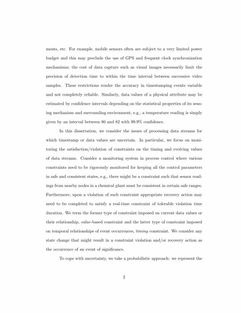
ments, etc. For example, mobile sensors often are subject to a very limited power
budget and this may preclude the use of GPS and frequent clock synchronization
mechanisms; the cost of data capture such as visual images necessarily limit the
precision of detection time to within the time interval between successive video
samples. These restrictions render the accuracy in timestamping events variable
and not completely reliable. Similarly, data values of a physical attribute may be
estimated by confidence intervals depending on the statistical properties of its sens-
ing mechanism and surrounding environment, e.g., a temperature reading is simply
given by an interval between 80 and 82 with 99.9% confidence.
In this dissertation, we consider the issues of processing data streams for
which timestamp or data values are uncertain. In particular, we focus on moni-
toring the satisfaction/violation of constraints on the timing and evolving values
of data streams. Consider a monitoring system in process control where various
constraints need to be rigorously monitored for keeping all the control parameters
in safe and consistent states, e.g., there might be a constraint such that sensor read-
ings from nearby nodes in a chemical plant must be consistent in certain safe ranges.
Furthermore, upon a violation of such constraint appropriate recovery action may
need to be completed to satisfy a real-time constraint of tolerable violation time
duration. We term the former type of constraint imposed on current data values or
their relationship, value-based constraint and the latter type of constraint imposed
on temporal relationships of event occurrences, timing constraint. We consider any
state change that might result in a constraint violation and/or recovery action as
the occurrence of an event of significance.
To cope with uncertainty, we take a probabilistic approach: we represent the
2

�������������� ������� ������������������������� ! "#�$�%&��� #���#%'()*+,-.( /-,- 0,+*-10 2344 56789:;<79=>;43;9<67:=83498?@?@?@
ABC/-,- 0D'+)*EFGHIJ KLMMHGNOP MQG FRJHSFIJTS QGUIFI VIWLHS32X;9=8 6Y :=;4Z[6:4X 6\]=598^Q_SFGIR_F SHF9:;5`<7a8=786: 8b89=c8
def0.)-g hD+g/ijklmnop
qHISLGHJH_FS QMGHIWrsQGWU QKtHuFS EH_SR_vJHuwI_RSJHGGQG JQUHW TGQKIKRWRSFRuUIFI uQ_SFGIR_FHVIWLIFRQ_Figure 1.1: A probabilistic monitoring system
uncertainty in object trace data probabilistically and specify a minimum probability
requirement to each constraint that denotes the confidence level of its violation or
satisfaction. Figure 1.1 sketches our architecture for a constraint monitoring system
where data sources (i.e., sensor nodes) track real-world objects in unpredictable
environments via error-prone sensing mechanism and generate continuous streams
of object trace data, and a stream processor constantly processes these data streams
to keep the constraint results up-to-date. Our approach to the issues of this system
is focussed specifically on the type of constraints to be monitored: timing constraint
or value-based constraint.
The first part of this dissertation proposes a probabilistic monitoring model
that incorporates temporal uncertainty into an event-based timing monitor. In
Chapter 2, we first present a generic framework Ptmon (probabilistic timing mon-
itor) [61] for monitoring timing constraints and capturing the early detection of
their violation. Monitoring timing constraints over events has been recognized as
an important issue in the area of real-time systems [11, 29, 45, 33]. In general, a
timing constraint defines a lower or upper bound on the time difference between
the event occurrences of interest. Given a set of such timing constraints as a part
3

xyz{|} ~�}�} ���� �� ���{�{��y�������{��{
�}����� ������ ������~�}��������������
Figure 1.2: Uncertainty of event occurrence times
of timing specification, an event monitor checks the constraints against an event
trace to detect their violation or satisfaction. In particular, detecting the violation
at the earliest time possible is desired since it allows users to take proper actions on
erroneous conditions in a timely manner [11, 45, 39].
Consider the following example illustrating an anomaly that arises when
events are correlated by using as input the time points at which the events are
detected from processing the data streams. This mode of event processing is said
to be by detection semantics. If the exact times of occurrence of the events are
known and are used as input, then we say that the mode of event processing is by
occurrence semantics. Unqualified use of the detection semantics can easily yield a
wrong answer where occurrence semantics is intended.
Example 1. Consider a constraint c stipulating that event e2 must occur within
60ms after the occurrence of event e1. Suppose that both sensors s1 and s2 have im-
perfect hardware that can incur errors in the timestamps that mark event detection.
Event e1 occurs at time=30 and event e2 occurs at time=150. However they are
detected and given timestamps equal to 70 and 120 respectively by sensors s1 and
s2, as shown in Figure 1.2. Notice that the constraint has indeed been violated and
should have been caught at time=90 but the violation is not detected in this case if
4

detection semantics applies.
As such, an event occurrence time may not be accurately known, but it is
often possible to represent it probabilistically by finding statistical properties of
individual sensing mechanisms via experiments and simulations [3].
By extending the run-time monitor models, temporal uncertainty was ad-
dressed in earlier work [46, 45] with the simplifying assumption that the occurrence
time of an event is uniformly distributed within a time interval [37]. There has also
been significant work from the database community to deal with the uncertainty
of time-varying objects in the context of probabilistic data and query execution
models [10, 13]. However, these models do not address the issue of correlating
the temporal relationship among data streams in order to determine whether cer-
tain timing constraint violation/satisfaction has occurred, which may in turn decide
whether the value of data attributes and occurrence times further down the data
stream are valid or not. We extend the problem of monitoring timing constraints
so as to cover a much broader class of models regarding timestamp uncertainty.
Based on the notion of probabilistic violation time, our framework provides a
systematic method for deriving the early detection of timing constraint violations.
We transform constraints between event occurrences into those between event de-
tections. We call such a transformed constraint a derived constraint, as opposed
to those that are explicitly given as a part of system specification. We also exploit
implicit constraints that can be inferred from a set of derived constraints in order to
monitor a constraint conjunction. An implicit constraint is considered necessary if
its violation can be detected earlier than any other constraints that will eventually
be violated. We note that the algorithm for identifying necessary implicit constraints
5

was first developed in the time point model [45]. Our framework distinguishes itself
from the past work (i.e., [29, 45, 44, 37, 43, 47]) in that it incorporates tempo-
ral uncertainty and is not limited to a specific probability distribution. Using the
proposed framework, we illustrate its applicability for different timestamp models.
The gaussian timestamp model can be used for various domains of monitoring data
streams where the physics of the noisy sensing mechanisms is well modelled. We
demonstrate that we can efficiently check the violation of timing constraints against
gaussian timestamps by exploring the graphs of probabilistic violation time with
respect to gaussian pdf (probability distribution function) parameters. In contrast,
the histogram timestamp model can be used when timestamp uncertainty is from
measurements only and may be represented by arbitrary probability distributions.
In this case, we show how to efficiently check the violation of timing constraints un-
der our framework. The framework allows the derivations to be done in a systematic
approach that can be followed like a recipe for other distributions. More specifically,
the framework leads to a timestamp-model-independent architectural layer that is
the core engine for conjunction compilation and run-time monitoring. Compiling
for some other distributions can thus be simplified as the implementation of the
function specified in Ptmon i.e., ge, pvt and pvw .
In Chapter 3, we also investigate a stream join operator Ptjoin (probabilistic
timing join) [47] of which join specification is based on temporal proximity as well
as temporal uncertainty. We show that the calculation of timing correlation shown
in Ptmon can be cast into a stream join operation that creates an output stream,
where each output tuple must satisfy the probability that the events in the join
specification occur together within a specified time interval. For efficiently checking
6

�� ¡¢£¤ ¥¦§ ©¦ª¨§£«¬¬ ®¯°±²³¬´²µ³´µ¶®¬²µ®¯¶·±¶
¸¹ ¸¹º»¼½º¾»¿ÀÁ»Â º»¼½º¾»¿ÀÁ»Â�à Ĥ§©ªÃŨƤ¢ ¥¦§¨©¦ª¨§£ÇÈÉÊËÌ ÍÉÎÏÊÇÇÎɶ®¯¬Ð ®¯³¯²Ñ¯®ÒÓÔÕÖ×ØÙÚÔÛÕÒÜÖÔÕ×ÚÔÖÕÚÒ°·±±³´µ¶®¬²µ ®¯¶·±¶·µ³¯®¬²µ¶®¯¬Ð¶°·¶Ý¸¹ ¸¹ ¸¹
¸¹Þ «¬¬ ¶´·®³¯
�ß àáâãä°·¶Ý å²±¯®¯« «¬¬¶®¯¬Ð¶ «¬¬ °®´æ¯ çèéê ·°«¬¯
ÇÈÉÊËÌ ÍÉÎÏÊÇÇÎɶ®¯¬Ð ®¯³¯²Ñ ®ÒÓÔÕÖ×ØÙÚÔÛÕÒÜÖÔÕ×ÚÔÖÕÚÒ °·±±³´µ¶®¬²µ ®¯¶·±¶¸¹ëìÀº ¸¹ëìÀºíî²±Þ ¯«ï¯ å²±¯®
ëìÀºèéêðñÖòÕØÒ×ÜÔÜóØÒ
¸¹Figure 1.3: Central Monitor, Edge Monitor, and Spmon
the Ptjoin condition upon event arrivals, we introduce the stream-partitioning
technique that delimits the probing range tightly. Ptjoin requires the detection of
timing constraint satisfaction, and so it can be seen as a dual problem of checking
timing constraint violations in Ptmon.
The second part of this dissertation addresses the problem of handling un-
certain data values and monitoring value-based constraints. This work is orthogonal
to that for accommodating uncertain timestamp values in event-based timing moni-
tors, which is covered by Ptmon and Ptjoin in the first part. As mentioned earlier,
a value-based constraint is in the form of range predicates on individual data values
or their relationships. In Chapter 4, we propose a new stream processing technique
Spmon (Similarity-based Probabilistic Monitoring) [58] which can incorporate un-
certainty in the monitoring of value-based constraints and reduce the amount of
data transmission from sensor nodes to a stream processor. More specifically, Sp-
mon considers the following problem: given a set of objects being tracked O, their
7
corresponding data streams capturing uncertainty of O in the form of time-varying
pdf s, and a set of user-specified value-based constraints C with confidence require-
ments, we want to monitor C over the data streams by updating the violation set
of C that contains all the violated constraints c ∈ C. Note that our approach can
be used for updating the satisfaction set that contains all the satisfied constraints
in C.
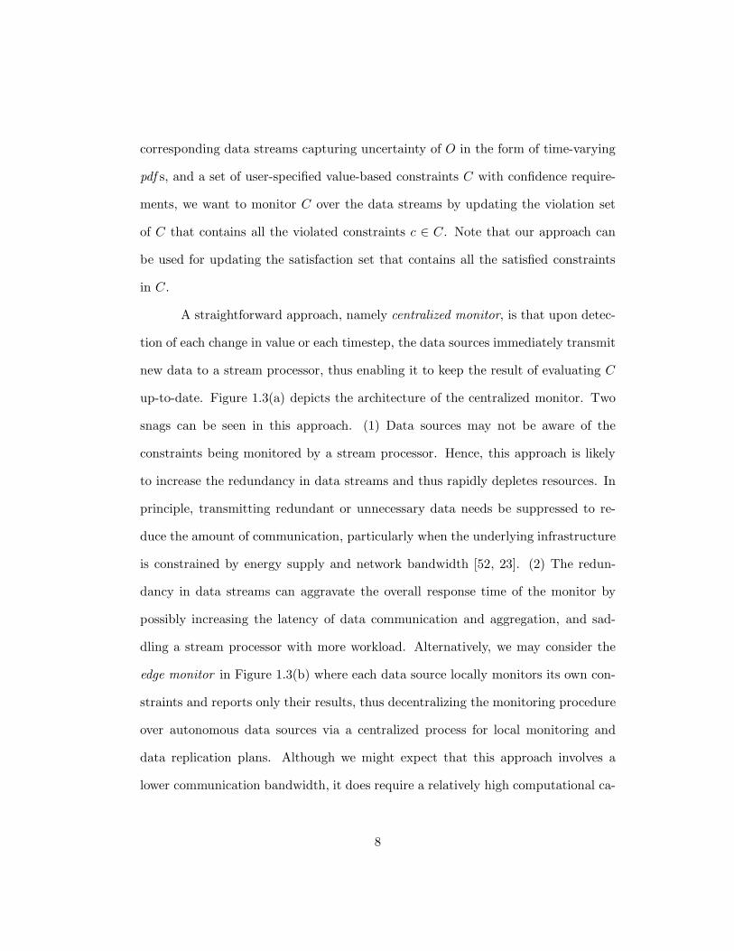
A straightforward approach, namely centralized monitor, is that upon detec-
tion of each change in value or each timestep, the data sources immediately transmit
new data to a stream processor, thus enabling it to keep the result of evaluating C
up-to-date. Figure 1.3(a) depicts the architecture of the centralized monitor. Two
snags can be seen in this approach. (1) Data sources may not be aware of the
constraints being monitored by a stream processor. Hence, this approach is likely
to increase the redundancy in data streams and thus rapidly depletes resources. In
principle, transmitting redundant or unnecessary data needs be suppressed to re-
duce the amount of communication, particularly when the underlying infrastructure
is constrained by energy supply and network bandwidth [52, 23]. (2) The redun-
dancy in data streams can aggravate the overall response time of the monitor by
possibly increasing the latency of data communication and aggregation, and sad-
dling a stream processor with more workload. Alternatively, we may consider the
edge monitor in Figure 1.3(b) where each data source locally monitors its own con-
straints and reports only their results, thus decentralizing the monitoring procedure
over autonomous data sources via a centralized process for local monitoring and
data replication plans. Although we might expect that this approach involves a
lower communication bandwidth, it does require a relatively high computational ca-
8

pacity for individual data sources. Moreover, monitoring constraints involving more
than a single data stream (e.g., monitoring the join relation on two objects for which
data values are captured by different remote sensor nodes) requires data replication
between data sources, which is often challenging in resource constrained environ-
ments. As such, both seemingly simple methods rely solely on either server-side
or source-side processing and both have limitations. Therefore, we take a different
approach to combine edge filters and a server-side monitor, and this is briefly illus-
trated in Figure 1.3(c); each data source monitors not user-specified constraints but
its filter, and a stream processor re-calculates the filter condition of data sources
upon the arrival of new data passing a filter.
In real-time databases, the consistency requirement of a transaction can be
relaxed in the sense that two different values of a database object are interchangeable
with respect to the transaction without incurring any undue effects if they are
similar [34, 7]. In general, two values of a database object are considered similar, if
their distance is within the deviation bound tolerance, and this is usually given by an
application designer as a part of the specification of the transactions referencing the
object. We adapt this notion of data similarity to the processing of uncertain data
streams. In doing so, we provide a systematic method to derive psr (probabilistic
similarity region) that specifies similarity relation on the pdf parameter space from
the semantics of given constraints.
Consider the example in Figure 1.4 (the detail is in Example 9-10 in Chap-
ter 4.1). We have a set of user-defined constraints over two objects o1 and o2 that
have the same type. Assume in this case the data values of o1 and o2 are given by
the gaussian distribution with different parameters, and accordingly each constraint
9

ôõö ÷õøõ ùõúûü ýþõÿ�ü���� �������� � � ��õøõ ùõúûü� �� ��� üýø� �� ��� ����� ! "#"$% & '
()*+,- .�+/0 1�2�3452 61�7589:;'&<$!=>!�>>?@"!$"�= &A ' A
Figure 1.4: Time-varying gaussian pdf s and psr -based filters
specification contains a given probability threshold. In figure(a), we have a pair of
gaussian distributions u and v that denote the estimate of o1 and o2 respectively
in timestep t1. As time progresses to the next timestep t2, we have new estimates
u′ and v′ for o1 and o2. Figure(b) depicts an example of psr as rectangles in the
2-dimensional (mean vs. standard deviation) space of gaussian pdf parameters. A
point in this space denotes a gaussian pdf. The gray (white) rectangle, the psr of
o1 (o2), depicts the area where any point (gaussian pdf ) is similar to u (v) with
respect to the given constraints. Notice that psr is not given by the user, but is
derived from the constraints. The derivation for psr will be shown in Chapter 4.
In figure(b), both estimates of o1 and o2 in timestep t2 are located within their
respective psr, ensuring that they do not affect the evaluation result of the given
10
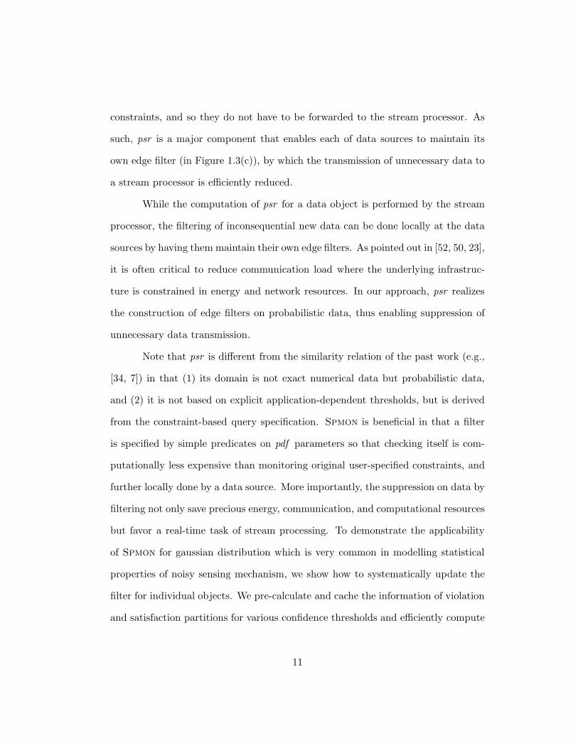
constraints, and so they do not have to be forwarded to the stream processor. As
such, psr is a major component that enables each of data sources to maintain its
own edge filter (in Figure 1.3(c)), by which the transmission of unnecessary data to
a stream processor is efficiently reduced.
While the computation of psr for a data object is performed by the stream
processor, the filtering of inconsequential new data can be done locally at the data
sources by having them maintain their own edge filters. As pointed out in [52, 50, 23],
it is often critical to reduce communication load where the underlying infrastruc-
ture is constrained in energy and network resources. In our approach, psr realizes
the construction of edge filters on probabilistic data, thus enabling suppression of
unnecessary data transmission.
Note that psr is different from the similarity relation of the past work (e.g.,
[34, 7]) in that (1) its domain is not exact numerical data but probabilistic data,
and (2) it is not based on explicit application-dependent thresholds, but is derived
from the constraint-based query specification. Spmon is beneficial in that a filter
is specified by simple predicates on pdf parameters so that checking itself is com-
putationally less expensive than monitoring original user-specified constraints, and
further locally done by a data source. More importantly, the suppression on data by
filtering not only save precious energy, communication, and computational resources
but favor a real-time task of stream processing. To demonstrate the applicability
of Spmon for gaussian distribution which is very common in modelling statistical
properties of noisy sensing mechanism, we show how to systematically update the
filter for individual objects. We pre-calculate and cache the information of violation
and satisfaction partitions for various confidence thresholds and efficiently compute
11

psr at run-time using these cached partitions.
The last part of this dissertation discusses our ongoing research issues. We
first introduce the hybrid monitoring technique [64] for resource-critical control-
oriented embedded systems. We also describe some extended functionalities in Pt-
mon and Spmon: (1) a generalized framework for probabilistic monitoring and fil-
tering of uncertain data streams to cover various types of probability distributions,
and to meet real-time requirements of a monitoring task by using adaptive monitor-
ing technique and data prediction models, and (2) a new stream join operator that
handles the intersection of uncertain period data.
1.2 Related Work
1.2.1 Event-based Monitoring
Much work on event-based monitoring systems has been done in the area of real-
time systems and active databases. In [11], Chodrow et al. presented the run-time
monitor model where system specifications expressed as invariant assertions in real-
time logics are constantly checked against event occurrences. The model includes
a graph-based monitoring scheme for catching the violation of invariant assertions
during the execution of time critical applications. In [46, 45], Mok and Liu devised
this run-time monitor model to improve its performance by exploiting the shortest
path graphs which can be constructed at the compilation time and the implicit
constraints which can expedite the violation detection of timing constraints. The
compilation algorithm for deriving a constraint graph containing all the necessary
constraints and the run-time algorithm for monitoring the constraint graph against
12

event occurrences were presented in [46] and the detail proofs for the correctness of
the algorithms were shown in [45]. This extended monitor model provides a distinct
advantage over the work by Chodrow et al. [11] in that it works in the complexity
O(n) at run-time where n is the number of time terms in a constraint in comparison
of the complexity O(n3) of [11].
Several composite event detectors e.g., [20, 19, 6] were proposed within trig-
ger systems of active databases, which enable databases to react to incoming events
or specific changes of database states. In general, composite event detectors have
similar specifications in the event-condition-action style; a trigger rule with event e,
condition c, and action a works as: upon the detection of e, c is evaluated against
the current database state, and if c holds, a is executed. On the contrary, they differ
in detection mechanism, for example, finite state automata in Ode [20], Petri-net
in SAMOS [19], event graphs in Sentinel [6]. While the event specification and de-
tection of the run-time monitor model above is based on event instances, that of
active databases is typically based on event types and event consumption policies
(e.g., parameter context [6]). Event consumption policies define semantics of event
composition by specifying which event instances should match the type-based argu-
ments in event operators and when they can expire. Owing to application-specific
properties of event consumption policies [43], active databases often become more re-
strictive in semantic clarity and extensibility of event operators than instance-based
models (e.g. [11, 46, 45]).
13

1.2.2 Monitoring with Uncertainty
As utility of wireless and embedded sensor technologies grows, event-based moni-
toring has become fundamental to today’s sensor-based applications. Here, we list
some of recent studies incorporating uncertainty in processing continuous streams
of sensor data, which are most closely related to the issues discussed in this disser-
tation.
In [44], Mok et al. proposed two qualitative modalities, possibly and certainly
in the run-time monitor model [46, 45] in order to handle uncertain event times-
tamps where each timestamp value is bounded in a time interval. These modalities
allow users to specify their certainty requirement by either non-zero possibility or
100% possibility for monitoring timing constraints over time intervals. In [37], the
assumption of uniform distribution on time intervals was made and accordingly the
algorithm for calculating the satisfaction probability of a timing constraint of two
time intervals was presented. We generalize this uncertainty-aware monitor model
and provide a probabilistic framework Ptmon by which we can capture the viola-
tion of a timing constraint over uncertain event occurrences at early stages and we
can adapt the monitoring functionalities to a broader range of uncertainty models
in a lightweight procedure. The approximate but histogram-like representation in
the context of valid-time indeterminacy has been used to express the probability
of the temporal data precedence, termed ordering plausibility [16]. The valid-time
indeterminacy is conceptually compatible with the notion of temporal uncertainty
of Ptmon. However, the target domain of valid-time indeterminacy is not a sensor-
based monitoring system but a temporal database. In the former, queries are re-
peatedly evaluated over high volume of data streams, but in the latter, queries are
14

once executed on temporal data, which are less frequently updated.
In recent years, various adaptive techniques in stream data management
have been proposed [30, 50, 52, 9, 2, 57]. In general, the tradeoff between the
quality of query results and the update frequency has been explored for achieving
either of two related goals: maximizing the precision of query results under the
resource limitation or minimizing the resource consumption while satisfying the
precision requirement. Particularly the work in [50, 52, 27, 9] can be categorized
as edge filtering on remote data sources. The edge filtering approach exploits the
specific query semantics (e.g., numerical aggregation queries with absolute precision
requirements [50], spatial range queries [27, 52], and entity-based queries [9]) for
efficient filter adaptation. In [27, 52], a safe region of objects being tracked is used for
efficiently monitoring spatial queries in the moving object database literature. A safe
region ensures the result of its associated spatial queries to remain unchanged as long
as a newly measured data value does not deviate from the safe region itself. While
none of these previous studies in edge filtering considered inherent uncertainty in
underlying data, our work Spmon specifically addresses the probabilistic models for
uncertain data together with the probabilistic semantics for constraint-based queries,
and concentrates on the efficient derivation of filter conditions for probabilistic data.
It is also important to note that we consider the probabilistic models only
for capturing the inherent imprecision in measurement data [8, 15, 24]. Such impre-
cision is generally incurred by error-prone sensing mechanisms independently from
the monitoring process. Thus our work differs from the approximate processing
(e.g., [50, 57]) that trades off the data quality for the query processing performance.
The notion of data similarity was originally introduced in the real-time
15

database literature to cope with the dynamics of real-world objects in real-time
environments, inasmuch as their updates are often captured with uncertainty but
those uncertain values are acceptably referenced by real-time transactions in a cer-
tain context. Especially, this similarity notion has been explored for relaxing the
data consistency requirements [34] and representing the flexible query semantics in
distributed real-time databases [7]. Work in [34, 7] only handled the uncertainty by
deterministic error bounds without the consideration of probability distributions of
underlying data. Our work Spmon is conceptually related with [34, 7], but it adapts
the similarity to pdf parameter spaces and furthermore exploits the given constraint
semantics for the derivation of local constraints on the pdf parameters of individ-
ual objects. As we described earlier, temporal uncertainty in the run-time monitor
model was first treated quantitatively [44] and later probabilistically [37, 61]. This
line of work has focused on the monitoring of timing constraints and accordingly
handled the temporal uncertainty of event streams, but not accommodated the
value uncertainty of data attributes contained in events. Therefore, Spmon can be
considered complementary to this prior work.
Data streams are unbounded and thus a stream operation needs to be re-
stricted with respect to its valid scope on input data streams. One common way is
to specify a time duration d and constantly keep a sliding window [tcur - d, tcur] on
data streams where tcur is the current system time. Significant work on data stream
research has been based on this sliding window mechanism [31].
While uncertainty regarding the transmission delay between data acquisition
and arrival to the stream processor has been considered for the sliding window mech-
anism in [22, 56], the issue of uncertain timestamps was not addressed. Particularly,
16

in [22], Hammad et al. introduced a sliding window join, so-called W-join, which can
handle the possible disorder and delay of data streams, given the assumption that
timestamp values of stream data are explicitly determined by remote data sources
with variable transmission capacity. This assumption is distinct from what typically
made in general stream join processing, that is, timestamp values of stream data
are implicitly consistent with their arrival time to a stream processor. Ptjoin can
be seen as one form of W-join operations, but its main concern is on the underlying
temporal uncertainty of event streams.
In the temporal database literature, many indexing structures for interval
data have been introduced. Efficient indexing structures are beneficial for imple-
menting temporal join operations if scanning the entire data stream is prohibitive
because of the database’s sheer size [17]. On the contrary, Ptjoin exploits statistical
properties of streams so as to improve the join performance and keep the necessary
index as simple. Indeed, in stream environments, a decision on selecting an index
structure should be made restrictively due to the high maintenance cost.
17

Chapter 2
PTMON: Probabilistic Timing
Monitoring
This chapter provides a comprehensive approach to the problem of monitoring tim-
ing constraints over event streams for which the timestamp values are inherently
uncertain and so they can be only given probabilistically. We propose a generic
probabilistic framework Ptmon by which the early detection of the violation of
timing constraints is made possible. To do so, we provide a systemic method for
deriving a set of necessary constraints at compilation time, using the notion of prob-
abilistic violation time. The framework is formulated to be modular with respect
to the probability model on uncertain timestamp values so that its implementa-
tion can be extended for different application requirements. We demonstrate the
applicability of the framework with different timestamp models.
18

2.1 A Probabilistic Framework for Monitoring Timing
Constraints
In this Chapter 2.1, we describe our framework for monitoring timing constraints
over event streams in probabilistic timestamp models.
2.1.1 Notations and Assumptions
A data stream A consists of a sequence of event occurrences (or simply, events)
{a1, a2, a3, . . .}. Events are detected by sensor nodes and transmitted to a data
stream processor.
Definition 1 (timing data). For an event ai, the timing data of ai, denoted by
ai.td, is a pair:
(ai.ts, ai.dt)
where ai.ts denotes the occurrence time of ai and ai.dt denotes the detection time
of ai.
Throughout this chapter, we make the following assumptions.
(1) The domain of time points is the set T P = R+ + {0}.
(2) For any event ai, its occurrence time is given by a pdf (probability distribution
function) and its detection time is given by a time point. We shall use the term
probabilistic timestamp1 to denote the probabilistic characterization of the occur-
rence time of an event. The timestamp of ai is made available at its detection time.
Accordingly, we assume that ai.dt = ∞ holds and ai.ts is not defined during at any
time t < ti, if ai has been detected at time point ti.
1For simplicity, we use timestamp to mean probabilistic timestamp throughout this chapter.
19
(3) The probability distributions associated with different event occurrences are in-
dependent of one another as in [16]. We emphasize that this assumption pertains
only to when within the time domain of its timestamp an event occurs, given that it
has been detected to occur within the time domain. The assumption is an assertion
about properties of the detection system, and not about the causes of the events
whose correlation is the subject of interest.
(4) If the degree of uncertainty of the occurrence time and the network delay of
events cannot be bounded, it is impossible to determine the violation or satisfaction
of a timing constraint. Henceforth, we consider only streams for which the tem-
poral uncertainty can be bounded. We use the term model parameter to denote a
parameter that applies as a bound for every event in a stream, to be detailed in
Chapter 2.2-2.3. We shall use M to denote a set of model parameters defined for
events and T DM to refer to the domain of timing data that satisfy all the parameters
in M.
Definition 2 (probabilistic timing relation, ge (≥) function). Given proba-
bilistic timestamps tsi, tsj and d ∈ R, we define the function ge as follows:
ge(tsi, tsj , d) = P (Xi + d ≥ Xj) =
∫
T PFj(t + d)fi(t)dt
where Xi and Xj are r.v. (random variable) on tsi and tsj respectively and Fj(t) =
P (Xj ≤ t) and fi(t) = P (Xi = t).
Note that timestamp arguments of the function ge above are each repre-
sented by their respective pdf in the definition. ge(.) is a basic function to define
the temporal relationship of two events. Most temporal operators in conventional
uncertain data models are formalized on top of such a temporal relationship.
20

Definition 3 (timing constraint). Given timing constraint
c : T1 + d ≥ T2
where T1, T2 are the time terms corresponding to the occurrence time of events and
d ∈ R (following the notation in [45]), we define probabilistic (timing) constraint
in the form of
(c, δ)
where 0 < δ < 1 is the confidence threshold [37]. P (X1 + d ≥ X2) is known as
the satisfaction probability of c where X1 and X2 are r.v. associated with T1 and T2
respectively. Let spc = P (X1 +d ≥ X2). The satisfaction of (c, δ) occurs if spc ≥ δ;
likewise, the violation of (c, δ) occurs if spc < δ.
2.1.2 Monitoring Probabilistic Constraints
As illustrated in [45], one of the main problems of monitoring timing constraints
is to find the inspection time point for expediting the violation detection of timing
constraints. Consider timing constraint c: a1.ts + 120 ≥ a2.ts. This asserts that
the occurrence of a2 is within 120 time units (i.e., ms) after the occurrence of a1.
Suppose that a1 occurs at time 100 but a2 does not by that time. In this case, c is
imposed on the occurrence of a1 with respect to the occurrence of a2 at runtime. If
uncertainty is not considered, i.e., ts is a time point, we can set up a timer expiring
at time 220 to detect the violation of c. The state of c must be unknown until time
220 unless a2 occurs by that time. This earliest time at which we can certainly
detect the violation of timing constraints is known as earliest violation time [45].
Now consider probabilistic constraint pc: (c, δ) in our probabilistic timestamp
model. If both a1 and a2 are detected by time 100, it is possible to determine the
21

violation or satisfaction of pc at no later than time 100 by calculating the satisfaction
probability of c, ge(a1.ts, a2.ts, 120). Like the previous example, suppose only a1 is
detected at time 100. In this case, owing to the absence of a specific timestamp of
a2, we cannot calculate the satisfaction probability of c until a2 is detected. With
a specific value of δ, however, it is only necessary to know whether the satisfaction
probability of c can exceed it or not in order to detect the violation of pc. Henceforth,
we consider the upper bound of the satisfaction probability of a timing constraint
and call the earliest time when it is impossible to meet the confidence threshold the
probabilistic violation time.
Definition 4 (pvt). Consider probabilistic constraint pc: (T1 + d ≥ T2, δ) and the
model parameter set M where T1 and T2 are time terms, d ∈ R, and 0 < δ < 1.
The probabilistic violation time of timestamp tsi is defined as follows:
pvt(tsi)|Mpc = max t s.t. ∃tsk ∈ S(t), ge(tsi, tsk, d) ≥ δ
where S(x) = {tsk|(tsk, dtk) ∈ T DM, dtk ≤ x}. Likewise, the probabilistic violation
time offset from time point tr is denoted by:
pvt(tsi, tr)|Mpc = pvt(tsi)|Mpc − tr.
Considering the domain set of possible timestamps where the detection time
is no later than some time point t, (denoted by S(t)), Definition 4 is meant to
capture the intuitive meaning of a probabilistic violation time. For example, given
probabilistic constraint pc: (a1.ts + d ≥ a2.ts, δ), the time point t1 = pvt(a1.ts)|Mpc
denotes the maximum possible time for the detection of a2 in order not to unavoid-
ably violate pc, provided a1.td, a2.td ∈ T DM. Put differently, t1 denotes the earliest
time at which we can detect the violation of pc during the period when a1 has been
22

detected but a2 has not. It should be noted that in practice, S(t) is not finite; it is
introduced only for the purpose of definition and not for implementation.
Theorem 1 (constraint derivation). Consider probabilistic constraint pc: (ai.ts+
d ≥ aj.ts, δ) where ai.td, aj .td ∈ T DM. A constraint cc
ai.dt + pvt(ai.ts, ai.dt)|Mpc ≥ aj .dt (2.1)
is said to be a derived constraint of pc. Clearly, cc is violated at time point t iff
t ≥ max(ai.dt, ti) ∧ aj .dt > ti where ti=pvt(ai.ts)|Mpc . For a probabilistic constraint
pc and its derived constraint cc, we have
violation of cc⇒ violation of pc.
Proof. Let ti = pvt(ai.ts)|Mpc . According to Definition 4, we have ge(ai.ts, ak.ts, d) <
δ for all ak such that ak.td ∈ T DM and ak.dt > ti.
Based on the notion of probabilistic violation time, Theorem 1 derives cc,
a timing constraint that is specified by the relationship of event detection times
given by time points from pc. Notice that cc is also a necessary constraint for pc,
particularly useful for catching its violation as early as possible. Accordingly, pc can
be evaluated at time point t in the following way:
satisfaction : if t ≥ max(ai.dt, aj .dt) ∧ spc ≥ δ
violation : if t ≥ max(ai.dt, aj .dt) ∧ spc < δ
: ∨ t ≥ max(ai.dt, ti) ∧ aj.dt > ti
unknown : otherwise,
where ti=pvt(ai.ts)|Mpc and spc=ge(ai.ts, aj .ts, d). The following algorithms encode
the monitoring method above particularly for detecting the violation of probabilistic
23

constraint pc. Algorithm 1 is invoked upon either the detection of events or the
expiration of a timer at time point t. Note that the algorithms contain the function
calls to ge(.) and pvt(.) and their implementation is timestamp model dependent.
They will be presented in Chapter 2.2 and 2.3.
Algorithm 1 checkPC (pc, cc, t)
1: // pc : probabilistic constraint (ai.ts + d ≥ aj .ts, δ)2: // cc : derived constraint of pc by Theorem 13: if checkTC (cc, t) = violation then4: violationHandler (pc)5: else if t ≥ max(ai.dt, aj .dt) ∧ δ > ge(ai.ts, aj .ts, d) then6: violationHandler (pc)7: end if
Algorithm 2 checkTC (cc, t)
1: // cc : ai.dt + pvt(ai.ts, ai.dt)|Mpc ≥ aj.dt2: if t = ai.dt ∧ t < aj .dt {upon the detection of ai} then3: // calculate probabilistic violation time offset4: time offset o← pvt(ai.ts, t)|Mpc
5: if o > 0 {set the timer} then6: set timer mcc at expiration time t + o7: else8: return violation9: end if
10: else if the expiration time of mcc = t ∧ t < aj.dt {upon the timer expiration}then
11: return violation12: end if
2.1.3 Monitoring Constraint Conjunctions
Consider a conjunction of timing constraints:
c1 : a1.ts + 100 ≥ a2.ts and c2 : a2.ts− 90 ≥ a3.ts
24

In case that uncertainty is not considered (i.e., time point model), we can find a
constraint c3: a1.ts + 10 ≥ a3.ts which makes it possible to detect the violation of
the conjunction early. For example, suppose a1 occurs at time 10 but neither a2
nor a3 occurs by time 20; then, c3 is violated at time 20 but neither of c1 nor c2
is violated at that time. Such a constraint being inferred from explicitly specified
constraints is known as an implicit constraint [45]. As such, monitoring implicit
constraints often expedites the violation detection. Now, consider a conjunction of
probabilistic constraints, (c1, 0.8) and (c2, 0.4). Finding implicit constraints, in this
case, is not as simple as that above since we need to consider uncertainty while
attempting to combine two constraints and to cancel the intermediate time term
being shared by the constraints.
Definition 5 (pvw). Consider probabilistic constraint pc: (T1 + d ≥ T2, δ) and the
model parameter set M where T1 and T2 are time terms, d ∈ R, and 0 < δ < 1.
The probabilistic violation window is defined by the time interval:
pvw |Mpc = [ min(tsk ,dtk)∈T DM
pvt(tsk, dtk)|Mpc ,
max(tsk,dtk)∈T DM
pvt(tsk, dtk)|Mpc ]
We denote the lower and the upper bound of probabilistic violation window v by lb(v)
and ub(v) respectively.
pvw |Mpc specifies the possible range of the probabilistic violation time offset
from the detection time of an event. Using this notion of probabilistic violation
window, we now present a way for inferring implicit constraints from a set of derived
constraints.
25

Definition 6 (implicit constraint). Given a conjunction Cec of probabilistic con-
straints, let Cdc be the set of derived constraints obtained from Cec by Theorem 1.
We call a constraint ccl
ccl : ai.dt + pvt(ai.ts, ai.dt)|Mpci+ Dl ≥ ak.dt (2.2)
an implicit constraint of Cdc if
cci : ai.dt + pvt(ai.ts, ai.dt)|Mpci+ Di ≥ aj.dt
and
ccj : aj .dt + pvt(aj .ts, aj .dt)|Mpcj+ Dj ≥ ak.dt
are derived constraints in Cdc or implicit constraints of Cdc where
Dl = Di + Dj + ub(pvw |Mpcj)
and pci, pcj are probabilistic constraints in Cec. Note that for any cci that is a
derived constraint but not an implicit constraint, Di = 0 holds.
Since Dl ≥ Di + Dj + pvt(aj .ts, aj .dt)|Mpcjnecessarily holds for any aj.td, we
obtain
violation of ccl ⇒ violation of cci ∧ ccj ⇒ violation of Cec.
More specifically, the violation of cci ∧ ccj implies the same for at least one derived
constraint in Cdc, regardless whether cci and ccj are derived constraints or implicit
constraints, and this in turn leads to the violation of at least one probabilistic
constraint in Cec by Theorem 1.
Monitoring a conjunction Cec of probabilistic constraints requires a multi-
step compilation task: (1) transforming the probabilistic constraints in Cec to the
26

corresponding derived constraints by using Theorem 1, (2) constructing a constraint
graph using the derived constraints, (3) adding edges to the constraint graph to in-
corporate the implicit constraints being generated according to Definition 6, (4)
eliminating unnecessary constraints. After completing this compilation task, we
obtain a necessary constraint set Cnc where each constraint is a derived constraint
or an implicit constraint for detecting the violation of Cec early. Each derived
constraint in Cnc and its paired probabilistic constraint in Cec can be monitored
together by Algorithm 1-2. Similarly, each implicit constraint in Cnc can be moni-
tored by Algorithm 2 with a simple modification: given an implicit constraint form
in Equation 2.2, the time offset in line 4 must be given by pvt(ai.ts, t)|Mpci+ Dl.
Since derived constraints are in the form of timing constraints between event
detection time points, they can be readily converted into the constraint graph rep-
resentation in step (2). A constraint graph consists a set of vertices corresponding
to the event detection times and a set of edges being annotated by time difference
between the vertices. We denote such a constraint graph that contains all the de-
rived constraints and all the implicit constraints by Gdc. Gdc is obtained in step
(3). It is noteworthy that every path in Gdc containing at least one intermediate
vertex corresponds to an implicit constraint. In step (4), based on the constraint
compilation method introduced in [45], we prune any constraints that are redundant
in terms of their timeliness for possible violations. However, owing to the fact that
every edge in Gdc is annotated by not a constant but a function of the timestamp
on its starting vertex (recall that pvt(.) function is contained in both Equation 2.1
and 2.2), we cannot directly use the time point based technique of [45].
In the following, we introduce a modified pruning technique for our prob-
27

abilistic model. Firstly, we prune every constraint that cannot possibly become a
shortest path of the vertex pair corresponding to the detection time pair of the
constraint. For any constraint ccl in the form of Equation 2.2, the lower and upper
bounds of its corresponding path length are given by
lb(pvw |Mpci) + Dl and ub(pvw |Mpci
) + Dl (2.3)
respectively. From these bounds, we can prune a constraint whose lower bound is
longer than the upper bound of some other constraint that has the same vertex
pair. We denote a constraint graph that contains only the candidate shortest paths,
Gsc. Secondly, we prune from Gsc every implicit constraint that is inferred from a
constraint pair for which a violation must occur no later than that of the implicit
constraint itself.
Theorem 2 (pruning). Consider constraints cci, ccj , and their implicit constraint
ccl in Definition 6. If
ub(pvw |Mpci) + Di ≤ 0 ∨ lb(pvw |Mpcj
) + Dj ≥ 0 (2.4)
then ccl can be pruned.
Proof. Given constraint c, let evt(c) be the earliest time at which c can be violated
and furthermore let ti = pvt(ai.ts)|Mpciand tj = pvt(aj .ts)|Mpcj
. We shall show that
either cci or ccj must be violated no later than evt(ccl) if ccl is violated; therefore, ccl
is redundant and can be pruned. Consider the condition that ub(pvw |Mpci) + Di ≤ 0
holds. In this case, we have
evt(ccl) = max(ai.dt, ti + Di + Dj + ub(pvw |Mpcj)),
evt(cci) = ai.dt,
evt(ccj) = max(aj .dt, tj + Dj)
28

regardless of the values of ai.ts and aj.ts. This is simply because we have evt(c) =
max(T1, T1+d) for any timing constraint c in the form: T1 +d ≥ T2. Now, suppose
ccl is violated at time evt(ccl), and so
ti + Di + Dj + ub(pvw |Mpcj) < ak.dt. (2.5)
Since evt(ccl) ≥ evt(cci) = ai.dt necessarily holds, we conclude that cci must be
violated no later than time evt(ccl) if cci is violated. Similarly, let us consider the
other case where cci is not violated at time evt(ccl), i.e, ti + Di ≥ aj.dt. From
Equation 2.5, we obtain aj .dt + Dj + ub(pvw |Mpcj) < ak.dt. Owing to the fact that
aj .dt + ub(pvw |pcj) ≥ tj necessarily holds, we obtain tj + Dj < ak.dt, which implies
evt(ccl) ≥ evt(ccj). The proof for the other condition (i.e., lb(pvw |Mpcj) + Dj ≥ 0) is
similar and is omitted.
2.2 Monitoring in Gaussian Timestamp Model
In Chapter 2.2, we describe the realization of the proposed framework in the gaus-
sian probability model. We consider timestamps that follow gaussian distribution
(namely, gaussian timestamp) and accordingly event streams with gaussian times-
tamps (namely, g-stream).
2.2.1 Gaussian Timestamp Model
For an event ai in g-stream A, we denote its gaussian timestamp by ai.ts = Gi:
(µi, σi) such that Xi ∼ N(µi, σ2i ) where Xi is r.v. on ai.ts. Thus, we have
P (Xi ≤ x) =
∫ x
−∞
1√2πσi
exp(−(y − µi)2
2σ2i
)dy
29
for Gi. Since no closed form solution exists for such an integral on gaussian distri-
bution, we use a well-known error function
Erf (x) =2√π
∫ x
0exp(−y2)dy
and the standard normal distribution function and its inverse function
Φ(x) = P (z ≤ x) =1
2(1 + Erf (
x√2)), Φ−1(Φ(x)) = x (2.6)
where z ∼ N(0, 1).
To realize the framework in the gaussian model, we first define model pa-
rameters and then provide the methods for computing ge(.) and pvt(.) functions.
Definition 7 (Gaussian timestamp). The following model parameters M =
{ω, κ,D} are defined for the gaussian model.
(1) ω is the model parameter that denotes the degree of uncertainty on the occurrence
time of events, i.e., for any gaussian timestamp Gi: (µi, σi), 0 < σi ≤ ω holds.
(2) κ is the model parameter that denotes the detection latency of events, i.e., for
any event ai with Gi: (µi, σi), ai.dt = µi + κσi holds. We assume that κ > 0 holds.
(3) D is the model parameter that denotes the network transmission delay of events,
i.e., any event ai is transmitted to a stream processor by time ai.dt+D. D is needed
to ensure that events are processed in the order of their detection time and the expi-
ration of a timer is delayed until the time by which the processing of all the events
detected no later than the expiration time of the timer has been completed.
Accordingly, the domain of timing data in g-streams, T DM is represented as
{((µk, σk), dtk)|µk, dtk ∈ T P , 0 < σk ≤ ω, dtk = µk + κσk}.
30

Throughout this Chapter 2.2, we shall suppose gaussian timestamps Gi:
(µi, σi), Gj : (µj , σj) and d ∈ R. Let us now consider the ge(.) function in Defi-
nition 2. By the linear transformation of gaussian distribution, we have
ge(Gi, Gj , d) = P (Xi + d−Xj ≥ 0) = 1− Φ(µj − µi − d)√
σ2i + σ2
j
) (2.7)
where Xi and Xj are r.v. associated with Gi and Gj respectively.
Example 2. Consider c: a1.ts + 110 ≥ a2.ts and δ = 0.9 where a1.ts = G1:
(100, 8), and a2.ts = G2: (200, 6). We obtain ge(G1, G2, 110) = 1−Φ(200−100−110)√82+62
)
= 1− Φ(−1) = 0.841 and thus (c, δ) is violated.
2.2.2 pvt in Gaussian Timestamp Model
In the following, we show how to compute pvt(.) in Definition 4 using the model
parameter set M = {ω, κ,D}. Consider probabilistic constraint pc in Theorem 1
and suppose pc is satisfied. Then, we have
ge(Gi, Gj , d) = 1− Φ(µj − µi − d√
σ2i + σ2
j
) ≥ δ
by Equation 2.7 and subsequently have
Φ(µj − µi − d√
σ2i + σ2
j
) ≤ 1− δ.
Due to the fact that Φ(x) < Φ(x + θ) necessarily holds for any x and θ > 0, we
obtain
µj − µi − d√
σ2i + σ2
j
≤ Φ−1(1− δ)
which is equivalent to
µj + κσj ≤ Φ−1(1− δ)√
σ2i + σ2
j + µi + d + κσj . (2.8)
31

Let v = Φ−1(1 − δ). Notice that Equation 2.8 denotes the upper bound of the
detection time of aj that can satisfy pc. Recall that pvt(.) ensures the violation for
any timestamp being detected after that time, and that it is calculated without a
specific timestamp of aj . Hence, we denote the right-hand side of Equation 2.8 by
a function of x = σj,
gt(x)|κGi,d,δ = v√
σ2i + x2 + µi + d + κx (2.9)
where 0 < x ≤ ω. From Equation 2.9, considering all the possible values of σj, we
finally obtain the following equation:
pvt(Gi)|Mpc = max0<x≤ω
gt(x)|κGi,d,δ (2.10)
We show examples of the graphs of gt(.) with various settings on κ (in Defi-
nition 7) and δ in Figure 2.1-2.2. In Figure 2.1, X-axis represents 0 < x = σj ≤ 50,
Y-axis represents 0 < κ ≤ 5, and Z-axis represents gt(x)|κGi,d,δ. And we set δ = 0.995,
Gi=(100, 8), and d=120. In Figure 2.2, X-axis represents 0 < x = σj ≤ 50, Y-axis
represents 0 < δ < 1, and Z-axis represents gt(x)|κGi,d,δ. And we set κ = 1.96,
Gi=(100, 8), and d=120.
In what follows, we explain how to find the maximum value of those graphs
for completing Equation 2.10.
First, consider the case when v ≥ 0 (equivalently, 0 < δ ≤ 12 ) holds. In this
case, gt(.) is a monotonic increasing function with respect to x = σj, and so we have
the following equation:
pvt(Gi)|Mpc = v√
σ2i + ω2 + µi + d + κω (2.11)
Second, consider the other case when v < 0 (equivalently 12 < δ < 1) holds. In this
case, the function gt(.) is not necessarily monotonically increasing, and so we find
32

010
20
30
40
500
1
2
3
4
5
100
200
300
010
20
30
40
Figure 2.1: gt(.) with various κ (detection latency) settings
010
20
30
40
50
0.2
0.4
0.6
0.8
100200
300
400
500
010
20
30
40
Figure 2.2: gt(.) with various δ settings
the upper bound of gt(.) by computing its derivative
dgt(x)|κGi,d,δ
dx= κ +
xv√
σ2i + x2
and a critical point,
x′ =σiκ√
v2 − κ2s.t.
dgt(x′)|κGi,d,δ
dx= 0.
If x′ is within the possible range of σj , that is
0 < x′ ≤ ω which is rewritten as δ ≥ Φ(κ
ω
√
ω2 + σ2i ), (2.12)
33

0.00.2
0.40.6
0.80
1020
3040
-100
0
100
200
300
400
500
Figure 2.3: An example graph of probabilistic violation time offset
then we obtain the following equation:
pvt(Gi)|Mpc = gt(σiκ√
v2 − κ2)|κGi,d,δ (2.13)
Otherwise, x′ > ω, and we have Equation 2.11 since in this case gt(.) is a monotonic
increasing function in the range of σj.
Theorem 3 (Gaussian pvt). The probabilistic violation time, pvt(Gi)|Mpc in Defi-
nition 4 can be calculated in the gaussian model as follows:
v√
ω2 + σ2i + µi + d + κω : if δ < Φ( κ
ω
√
ω2 + σ2i )
σi(κ2−v2)√
v2−κ2+ µi + d : otherwise,
where v = Φ−1(1− δ).
Proof. By Equation 2.11 and 2.12, we obtain the first formula for the case that
0 < δ < 12 = Φ(0) < Φ( κ
ω
√
ω2 + σ2i ). Similarly, we obtain the second formula by
Equation 2.12 and 2.13.
34

Example 3. Figure 2.3 shows the graph of probabilistic violation time offset
pvt(ai.ts, ai.dt)|Mpc where pc: (ai.ts + 120 ≥ aj.ts, δ), κ=1.96, and ω=50 are given.
In the figure, X-axis represents 0 < δ < 1, Y-axis represents 0 < σi ≤ ω, and Z-axis
represents probabilistic violation time offset. We find the derived constraint cc where
the time difference between the time terms is given by this time offset function of
ai.ts by Theorem 1 for a specific value of δ. For example, suppose δ = 0.8, ai is
detected at time 119.6 and its timestamp is given by Gi: (100, 10). Then, we obtain
δ = 0.8 < Φ( κω
√
ω2 + σ2i ) = 0.98 and accordingly, the time offset, pvt(ai.ts, ai.dt)|Mpc
= pvt(ai.ts)|Mpc − ai.dt = 155.5 by using the first formula in Theorem 3, as marked
in the graph. Hence, a deadline timer can be set to expire at time 275.1 for checking
the violation of cc upon the detection of ai as in Algorithm 2.
2.2.3 Computing pvw
As shown in Chapter 2.1.3, monitoring a constraint conjunction requires the calcu-
lation of probabilistic violation windows. Here we present the calculation for the
gaussian model.
Theorem 4 (Gaussian pvw). Consider a probabilistic violation window pvw |Mpc
in Definition 5 in the gaussian model. Let
g1(x) = v√
x2 + ω2 − κx + d + κω,
g2(x) =x(κ2 − v2)√−κ2 + v2
− κx + d
35
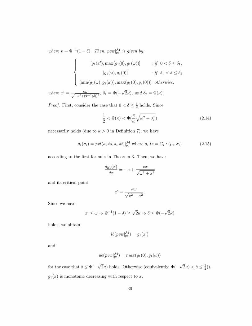
where v = Φ−1(1− δ). Then, pvw |Mpc is given by:
[g1(x′),max(g1(0), g1(ω))] : if 0 < δ ≤ δ1,
[g1(ω), g1(0)] : if δ1 < δ ≤ δ2,
[min(g1(ω), g2(ω)),max(g1(0), g2(0))]: otherwise,
where x′ = κω√−κ2+(Φ−1(δ))2
, δ1 = Φ(−√
2κ), and δ2 = Φ(κ).
Proof. First, consider the case that 0 < δ ≤ 12 holds. Since
1
2< Φ(κ) < Φ(
κ
ω
√
ω2 + σ2i ) (2.14)
necessarily holds (due to κ > 0 in Definition 7), we have
g1(σi) = pvt(ai.ts, ai.dt)|Mpc where ai.ts = Gi : (µi, σi) (2.15)
according to the first formula in Theorem 3. Then, we have
dg1(x)
dx= −κ +
vx√ω2 + x2
and its critical point
x′ =κω√
v2 − κ2.
Since we have
x′ ≤ ω ⇒ Φ−1(1− δ) ≥√
2κ⇒ δ ≤ Φ(−√
2κ)
holds, we obtain
lb(pvw |Mpc ) = g1(x′)
and
ub(pvw |Mpc ) = max(g1(0), g1(ω))
for the case that δ ≤ Φ(−√
2κ) holds. Otherwise (equivalently, Φ(−√
2κ) < δ ≤ 12)),
g1(x) is monotonic decreasing with respect to x.
36

Second, consider the case 12 < δ ≤ Φ(κ). By Equation 2.14, we have Equa-
tion 2.15 and g1(x) is monotonic decreasing in the valid range of x as explained
previously.
Finally, consider the case Φ(κ) < δ < 1. As discussed in the if -condition
of Theorem 3, Equation 2.15 does not always hold in this case. Hence, we need
to find pvw |Mpc by comparing the lower and upper bounds of both g1(x) and g2(x).
As shown before, g1(x) is monotonic decreasing for the case δ > Φ(κ) > Φ(−√
2κ).
Now consider g2(x). Since we have
δ > Φ(κ)⇒ Φ−1(δ) > κ⇒ Φ−1(1− δ) < −κ
holds, g2(x) is also monotonic decreasing in this case.
In Figure 2.4, we show an example set of derived and implicit constraints after
the compilation in the gaussian model. In figure(a) we have a graph representation
for 6 probabilistic constraints among the occurrences of 5 events and in figure(b) we
obtain a set of necessary derived/implicit constraints among the detection times of
the events being found via the compilation task in Chapter 2.1.3. Notice 3 implicit
constraint are inferred from the example conjunction of 6 probabilistic constraints,
but two of them can be pruned.
Example 4. In Figure 2.4, we illustrate an example set of derived and implicit con-
straints after compilation in the gaussian model with ω = 20, κ = 1.96. Figure 2.4(a)
illustrates the constraint graph representation of a conjunction of 6 probabilistic con-
straints over events a1-a5. An annotated triple (pci, d, δ) on each edge denotes a
probabilistic constraint between the pair of event occurrence times that correspond to
the starting/ending vertex in the constraint graph, e.g., pc1: (a1.ts+80 ≥ a2.ts, 0.6)
37

BCDEF EGEHEI
EJKLMNOPOQP RS TUVWXYVZ[\] _ a bccdceTfgVWZYfX\ hij ki lmn kjopqrrstu qvrswxpyrswu z{s{x
|}~��}�~��� ��� �� ��� �������������
����� ������
��� ¡¢£¤¢¥¦§¤ ¨©ª¢«¬¤¢¥¦¨©®¢¯¥¢¥¦ ¤¨©°¢§¥¢¥¦¬ ¨©±¢«²¥¢¥¦¨©³¢ ¥¢¥¦ §
Figure 2.4: An example of compilation
by the edge between a1 and a2. In Figure 2.4(b), derived constraints (by Theorem 1)
and implicit constraints (by Definition 6) are denoted by solid and dotted lines re-
spectively. An annotated pair on each edge denotes the lower and upper bounds of
the probabilistic violation time offset from the start vertex (Equation 2.3). Unlike
those in Figure 2.4(a) that correspond to the occurrence time of events, the vertices
correspond to the detection time of events. The implicit constraint covering the path
38

a1, a3, a4, a5 is pruned because it cannot become a shortest path (since 103 > 97.7).
And the implicit constraint covering the path a3, a4, a5 is pruned by Theorem 2.
2.3 Monitoring in Histogram Timestamp Model
In Chapter 2.3, we show how to realize the framework for event streams with his-
togram timestamps [47], namely h-stream.
2.3.1 Histogram Timestamp Model
We use the symbol I to denote a time interval I = [t1, t2] where t1 and t2 are
time points such that t1 < t2. The following auxiliary functions are defined for
time intervals: lb(I) = t1, ub(I) = t2, x ∈ I iff lb(I) ≤ x ≤ ub(I), and I + x =
[lb(I) + x, ub(I) + x] for any x ∈ R. For a event ai in h-stream A, we denote its
histogram timestamp by
ai.ts = Hi : ((Ii1, pi1), (Ii2, pi2), . . . , (Iin, pin))
where (Iik, pik) is called the kth bucket such that P (Xi ∈ Iik) = pik and Xi is r.v.
on ai.ts. Every histogram timestamp Hi has the following properties:
(1)∑n
k=1 pik = 1,
(2) ∀1 ≤ k < n, ub(Iik) = lb(Iik+1),
(3) ∀1 ≤ k ≤ n, the occurrence time is uniformly distributed over each Iik. Formally,
pdf is described by f(x) = pik
ub(Iik)−lb(Iik) if x ∈ Iik.
We have the following auxiliary functions:
(1) |Hi| = the number of buckets n,
(2) lb(Hi) = lb(Ii1),
39

(3) ub(Hi) = ub(Ii|Hi|),
(4) len(Hi) = ub(Hi)− lb(Hi),
(5) Hi + x = ((Iik + x, pik))1≤k≤|Hi| for any x ∈ R. To realize the framework in the
histogram model, we first define the model parameters and then provide the method
for computing ge(.) and pvt(.) functions.
Definition 8 (Histogram timestamp). The following model parameters M =
{τ,H,D} are defined for the histogram model.
(1) τ is the model parameter that denotes the detection latency of events, i.e., for
any event ai, ai.dt = lb(Hi) + len(Hi)τ where Hi = ai.ts.
(2) H = {φ1, φ2, . . . , φn} is the model parameter that denotes the set of template
histograms2. More specifically, we assume that for every event, a stream processor
can determine its own histogram timestamp by shifting its associated template his-
togram that is a priori known. For example, suppose that event ai is detected at time
ti by a sensor node sl that is observed to empirically satisfy a probability distribution
represented by the template histogram φl ∈ H with respect to the detection latency
of its sensing modality. Then, upon the arrival of ai, a stream processor can capture
Hi = φl + (ti − lb(φl)− len(φl)τ) (2.16)
for the timestamp of ai. We may write Hi ≃ φl to denote such a relation of times-
tamp Hi and its template histogram φl.
(3) D is same as that in Definition 7.
2For clarity, the symbol φ is used to denote a template histogram that represents a pdf when the
the associated event is not named.
40

µ¶·¸¹º»¼½¼¾½¿ÀÁ Âà ÄÅÆÇ ÈÇ ÉÇÊÇ ËÇÌÇ ÍÇÇ ÍÍÇÎÇ ÍËÇ ÊÇÇ ÊÍÇÍÎÇ¹Ï »¼½¼¾½¿ÀÁ Âà ÄÐ ¹Ñ»¼½¼¾½¿ÀÁ Âà ÄÅFigure 2.5: An example of h-streams
Accordingly, the domain of timing data in h-streams is represented as
T DM = {(φk + t, dtk)|φk ∈ H, dtk ∈ T P, t ∈ R,
dtk = lb(φk) + t + len(φk)τ, t ≥ −lb(φk)}.
The following example illustrates how we can capture the histogram times-
tamp of an event by using the template histogram that models the detection latency
of the event. For clarity, we shall use the symbol φ to denote a template histogram
that represents a pdf when the the associated event is not named. Without loss of
generality, we assume that lb(φi) = 0 for all template histograms φi.
Example 5. Consider a stream A consisting of events from multiple sensor nodes
s1, s2, . . . , sn where a sensor node si is observed to empirically satisfy a probabil-
ity distribution represented by the template histogram φi = ((Ii1, pi1), . . . , (Iim, pim))
with respect to the detection latency of its sensing modality for i = 1, . . . , n. For
example, suppose the detection latency of s1 satisfies the distribution
((0, 10, 0.6), (10, 20, 0.3), (20, 40, 0.1)). Note that here a bucket may be written in a
triple without the inner brackets enclosing its time interval. So the template his-
togram of s1 is defined as φ1 = ((0, 20, 0.1), (20, 30, 0.3), (30, 40, 0.6)). In this case,
for an event aj that is detected at time tdet by s1, the data stream processor can
probabilistically approximate the occurrence time of aj by Hj = φ1 + tdet − ub(φ1).
41

Figure 2.5 depicts three timestamps captured from two sensor nodes, i.e., s1 detects
two events a1 and a3 at time 60 and 210, and s2 detects an event a2 at time 110
where φ2 = ((0, 10, 0.15), (10, 20, 0.3), (20, 30, 0.4), (30, 40, 0.15)).
Here let us consider ge(.). Suppose we have histogram timestamps Hi, Hj
and let Xi, Xj be r.v. associated with Hi, Hj respectively. Then, ge(Hi,Hj, d) can
be expressed as|Hi|∑
u=1
|Hj |∑
v=1
P (Xi + d ≥ Xj ,Xi ∈ Iiu,Xj ∈ Ijv) (2.17)
which sums up the probability contributions from all the possible interval pairs. In
order to compute Equation 2.17 efficiently, we use histogram adjustment [47].
Definition 9 (adjusted histogram). Let Ti=lb(Ii1),lb(Ii2),. . .,lb(Iin), ub(Iin) be
the list of the time points in Hi and let Tj = lb(Ij1), lb(Ij2),. . . ,lb(Ijm), ub(Ijm)
where n=|Hi| and m=|Hj|. By merging Ti and Tj in ascending order without rep-
etition of any equal time points, we obtain a list of time points t1 < t2 < . . . <
tl < tl+1 and construct the time intervals I1 = [t1, t2], . . . , Il = [tl, tl+1]. The his-
togram consisting of the buckets (I1, P (Xi ∈ I1)),. . . ,(Il, P (Xi ∈ Il)) will be called
the adjusted histogram of Hi and similarly the histogram consisting of the buckets
(I1, P (Xj ∈ I1)),. . . ,(Il, P (Xj ∈ Il)) will be called the adjusted histogram of Hj.
Given two histogram timestamps Hi and Hj, let Hi = ((Iu, piu))1≤u≤l and
Hj = ((Iv, pjv))1≤v≤l be the adjusted histograms of Hi + d and Hj respectively,
where |Hi| = |Hj | = l. Then, we have [35, 47]
ge(Hi,Hj , d) =
l∑
u=1
u−1∑
v=1
piupjv +1
2
l∑
u=1
piupju. (2.18)
Notice that the complexity of calculating ge(Hi,Hj, d) is O(|Hi|+ |Hj|). The time
required for shifting a histogram timestamp and acquiring the adjusted histograms
42

is linear with respect to the number of buckets in the same way as merging two
sorted lists. Algorithm 3 implements Equation 2.18. As can be seen, its complexity
is also linear with respect to the number of buckets.
Algorithm 3 calGE (Hi, Hj)
1: cp← 0, prob← 02: for u = 1 to |Hi| do3: prob← prob + piucp + 1
2 piupju
4: cp← cp + pju
5: end for6: return prob
2.3.2 pvt in Histogram Timestamp Model
In the following, we show how to compute pvt(.) with M = {τ,H,D}. Let us first
define the following function on a histogram pair:
ht(φi, φj , δ) = t s.t. ge(φi, φj , tj − t) = δ (2.19)
where t ∈ R and tj = lb(φj) + len(φj)τ . It is clear that for any d ∈ R, we have
ht(φi, φj , δ) + d = ht(φi + d, φj , δ). (2.20)
Let Tiu and Tjv be the list of the time points in φi and φj where u=1 . . . n + 1,
v=1 . . . m+1, n=|φi| and m=|φj | as in Definition 9. We use the term configuration to
denote a tuple (y1, y2, . . . , ym+1) where yk = 0 if Tjk < Ti1, yk = l if Til ≤ Tjk < Til+1
(1 ≤ l ≤ n), and yk = n + 1 if Tjk ≥ Tin+1 for k = 1, . . . ,m + 1. A straightforward
approach for computing ht(.) is to enumerate all possible configurations that pertain
to φi and φj+x by increasing x where lb(φi)−ub(φj) ≤ x ≤ ub(φi)−lb(φj) in order to
find the bounding configuration such that ge(φi, φj ,−x) = δ. For each configuration,
43

we compute the lower and upper bounds of ge(φi, φj ,−x). Let δ1 = ge(φi, φj , d) for
some d ∈ R and suppose 0 < δ1 < 1. Then the inequality
ge(φi, φj , d− θ) < δ1 < ge(φi, φj , d + θ) (2.21)
necessarily holds for any θ > 0 according to the formula in Definition 2. Therefore,
the bounds of ge(φi, φj ,−x) are achieved by calculating ge(φi, φj ,−x) with the
minimum and maximum possible values of x in a configuration.
In practice, we can find the configuration bounding δ efficiently by using
binary search, delimiting the range of x into
max(lb(φi)− tj, ti − ub(φj)) ≤ x ≤ min(ub(φi)− tj, ti − lb(φj))
where Xi, Xj are r.v. on φi, φj respectively, and ti, tj are the time points such
that P (Xi ≤ ti) = 1 − δ, P (Xj ≤ tj) = δ respectively. In particular, this method
efficiently prunes unnecessary configurations in case the number of buckets in his-
tograms is large. Once the configuration bounding δ is identified, we can formulate
the quadratic equation corresponding to ge(φi, φj ,−x) = δ in the configuration. Fi-
nally, we obtain ht(φi, φj , δ) = x+ lb(φj)+ len(φj)τ exactly by solving the quadratic
equation for x.
Theorem 5 (Histogram pvt). The probabilistic violation time, pvt(Hi)|Mpc in Def-
inition 4 can be calculated in the histogram model as follows:
maxφk∈H
ht(φl, φk, δ) + d + ti (2.22)
where Hi ≃ φl and ti = lb(Hi)− lb(φl).
Proof. Let t1=ht(φl, φh, δ)+d+ti and th = lb(φh)+len(φh)τ for a template histogram
φh ∈ H. Then, we have t1=ht(Hi + d, φh, δ) (by Equation 2.20) and subsequently
44

ge(Hi + d, φh, th − t1)=δ (by the definition in Equation 2.19). Now, consider a time
point t2 > t1. We have that ge(Hi+d, φh, th−t2) < δ necessarily holds for any t2 > t1
by Equation 2.21. Similarly, for any time point t3 ≤ t1, we have ge(Hi+d, φh, th−t3)
≥ δ. Thus, t1 is the maximum possible time for the detection of event aj in order
to satisfy pc in the case of aj.ts=Hj ≃ φh. So, we have the following inequality
aj.dt ≤ t1 = ht(φl, φh, δ) + d + lb(Hi)− lb(φl)
for satisfying pc. Obviously, pvt(.) must be calculated based on not a specific dis-
tribution but all the possible distributions for the timestamp of aj. By exploiting
the set of template histograms given, Equation 2.22 realizes the formula in Defini-
tion 4.
Notice that given H and a specific value of δ, we can pre-compute ht(φi, φj , δ)
for all pairs of template histograms φi, φj ∈ H so as to find the probabilistic violation
time for a histogram timestamp in constant time upon the arrival of events at
runtime.
Example 6. Consider the satisfaction time ht(H3,H2, 0.8) where H2 and H3 are
the histogram timestamps of a2 and a3 in Example 5. From ge(H3,H2,−90) = 0.925
and prob(H3,H2,−100) = 0.769, we obtain the bounding configuration (0, 1, 1, 2, 3)
for ge(H3,H2,−x) = 0.8 where 90 ≤ x < 100. Let y = lb(H2) + x = 70 + x and
H ′2 = H2 + x = H2 + y − 70 for notational convenience, and we obtain the adjusted
histograms H3 = ((I1, 0), (I2, 0.005y−0.8), (I3 , 0.05), (I4,−0.005y+0.85), (I5 , 0.03y−
4.8), (I6,−0.03y+5.1), (I7, 0.06y−9.6), (I8 ,−0.06y+10.2)) and H ′2 = ((I1,−0.015y+
2.55), (I2, 0.015y− 2.4), (I3, 0.3), (I4,−0.04y +6.8), (I5, 0.04y +−6.4), (I6,−0.015y +
2.55), (I6, 0.015y−2.4), (I7 , 0)) of H3 and H ′2 respectively where Ik = [y, 170], [170, y+
45

10], [y + 10, y + 20], [y + 20, 190], [190, y + 30], [y + 30, 200], [200, y + 40], [y + 40, 210]
for k = 1, . . . , 8. Then we have
ge(H3,H′2, 0) =
8∑
u=1
u−1∑
v=1
p3up2v +1
2
8∑
u=1
p3up2u
= −0.0007625y2 + 0.236y − 17.315 = 0.8
where p3u and p2v denote the probabilities in H3 and H ′2. By solving the equation,
we have y = 168.59 and subsequently we have ht(H3,H2, 0.8) = x + ub(H2) =
y − lb(H2) + ub(H2) = 168.59 − 70 + 110 = 208.59.
2.3.3 Computing pvw
The following theorem shows how to calculate pvw in the histogram model.
Theorem 6 (Histogram pvw). Consider a probabilistic violation window pvw |Mpc
in Definition 5 in the histogram model. Let
h(H) = pvt(H)|Mpc − lb(H)− len(H)τ
for the histogram H. Then, pvw |Mpc in Definition 5 is given by
[ minφk∈H
h(φk), maxφk∈H
h(φk)].
Proof. The proof should be obvious and is omitted.
2.4 Monitoring in Uniform Timestamp Model
The interval model in [37, 35] is a single bucket histogram (e.g., Hi : ((Ii1, 1.0)))
where the timing uncertainty is uniformly spread out within an interval. Due to the
46

simplified assumption of the interval model, the computation required for checking
the temporal relationship of events can be much less complex than that of the
histogram model. Here we generalize the interval model by following the Ptmon
framework and removing the assumption (made in [37, 35]) such that an event
is detected only at the upper bound of its interval timestamp. We rather exploit
a model specifying the relationship between event occurrences and detections by
model parameters.
2.4.1 Uniform Timestamp Model
We use the symbol U to denote a uniform timestamp (or a single bucket histogram).
We call such an event stream with uniform timestamps u-stream. The auxiliary
functions defined for intervals are used in the same way for uniform timestamps:
lb(Ui) = i1, ub(Ui) = i2, len(Ui) = i2 − i1, Ui + x = [i1 + x, i2 + x] for Ui: [i1, i2]
and x ∈ R.
Definition 10 (Uniform timestamp). The following model parameters M =
{τ, π, ρ,D} are defined for the uniform model.
(1) τ is the detection latency parameter defined similarly as that in Definition 8,
i.e., for any event ai, ai.dt = lb(Ui) + len(Ui)τ where Ui = ai.ts. We assume that
12 ≤ τ ≤ 1 holds.
(2) π and ρ are the model parameters that denote the maximum and the minimum
length of uniform timestamps, i.e., ∀Ui, ρ ≤ len(Ui) ≤ π.
(3) D is the delay parameter defined same as that in Definition 7.
Accordingly, the domain of timing data in u-streams is represented as
T DM = {([i1, i2], dtk)|i1, i2, dtk ∈ T P , ρ ≤ i2 − i1 ≤ π, dtk = i1 + (i2 − i1)τ}.
47

The ge(.) function for uniform timestamps is established based on the con-
figurations possibly made by two intervals. Note that the notion of configurations is
explained in Chapter 2.3.2. The six different cases in the below lemma correspond
to the configurations (2, 2), (0, 0), (1, 2), (1, 1), (0, 1), and (0, 2) respectively.3
Lemma 1. Given Ui = [i1, i2] and Uj: [j1, j2], we have
ge(Ui, Uj , d) =
0 : if i′2 ≤ j1,
1 : if j2 < i′1,
(i′2−j1)2
2(i′2−i′
1)(j2−j1)
: if i′1 ≤ j1 < i′2 ∧ i′2 ≤ j2,
(2i′2−j1−j2)
2(i′2−i′
1) : if i′1 ≤ j1 ∧ j2 < i′2,
1− (j2−i′1)2
2(i′2−i′
1)(j2−j1)
: if j1 < i′1 ∧ i′1 ≤ j2 < i′2,
(i′2−2j1+i′
1)
2(j2−j1): otherwise
where i′1 = i1 + d and i′2 = i2 + d.
Proof. Since the proof for non-overlapping intervals is straightforward, here let us
show the proof for the cases when Ui +d and Uj overlap. We can divide the timeline
on Ui + d into three subintervals: Ia where Ui + d definitely precedes Uj, Ib where
Ui + d and Uj intersect, and Ic where Ui + d definitely follows Uj .
Let us use Xi and Xj for r.v. on Ui + d and Uj. Consider the third case
(configuration (1, 2)). We find Ia and Ib but not Ic. Since there is no way to satisfy
Xj < Xi in Ia, we only need to consider the probability in Ib = [j1, i′2] such that
P (Xi ≥ Xj |Xi ∈ Ib,Xj ∈ Ib)(Xi ∈ Ib)(Xj ∈ Ib) =P (Xi ∈ Ib)P (Xj ∈ Ib)
2.
This is because we have
P (Xi ≥ Xj |Xi ∈ Ib,Xj ∈ Ib) =1
len(Ib)2
∫ ub(Ib)
lb(Ib)t− lb(Ib)dt =
(ub(Ib)− lb(Ib))2
2 · len(Ib)2=
1
2.
3While in [37, 35] the configurations are notated by α, β, and γ, we uses the numbers to beconsistent with the histogram model.
48

Owing to the uniform distribution on each time interval, the probability for subin-
tervals can be easily calculated by P (Xi ∈ Ib) = len(Ib)len(Ui)
and P (Xj ∈ Ib) = len(Ib)len(Uj)
.
Similarly let us consider the fourth case (configuration (1, 1)). In addition to the
probability in the overlapping interval Ib = [j1, j2], we need to add the probability
in the interval Ic = [j2, i′2] where Xi ≥ Xj always holds. We obtain that
P (Xi ∈ Ic)P (Xi ≥ Xj|Xi ∈ Ic) =len(Ic)
len(Ui).
Then we sum the contribution from Ib and Ic, that is,len(Uj)2len(Ui)
+ len(Ic)len(Ui)
. The other
cases can be similarly established. In particular, we can derive the formula for the
fifth case (the sixth case) from that of the third case (the fourth case) using the
inverse relation, i.e., P (Xi ≥ Xj) = 1− P (Xj ≥ Xi).
In the following, we show how to compute the uniform pvt(.) with the model
parameter set M = {τ, π, ρ,D} in Definition 10.
2.4.2 Maximum Probability with Different Configuration Cases
To get the uniform pvt(.), we first analyze the property of the ge(.) function in differ-
ent configurations. More specifically, we derive the upper bound of the ge(.) function
over time when Ui in the constraint calculation, e.g., ge(Ui, Uj , d), is resolved but
Uj is not.
Recall that we focus only on the case of 12 ≤ τ ≤ 1, as described in Defini-
tion 10. The other cases can be established similarly as the derivations introduced
here. It is obvious that we have Ui +d = [i1 +d, i2 +d] for any Ui: [i1, i2] and d ∈ R,
thus we assume d = 0 for simplicity. And we use a timestamp variable denoted by
t and l,
Ut : [t− τ l, t + (1− τ)l] (2.23)
49

where t is the detection time of Ut and l is the length of Ut.
Configuration (1, 2) case. Given Ui: [i1, i2] and Ut (Equation 2.23), for the con-
figuration (1, 2), the ge(.) can be rewritten as the function of the length l of Ut by
using the corresponding third formula in Lemma 1:
sp(1,2)(l)|τUi,t= ge([i1, i2], [t− τ l, t + (1− τ)l], 0) = −(i2 + lτ − t)2
2l(i1 − i2). (2.24)
The condition of the configuration (1, 2) regarding the valid range of l is given by
i1 ≤ t− τ l < l2 ∧ i2 ≤ t + (1− τ)l ⇒ max(t− i2τ − 1
,t− i2
τ) ≤ l ≤ t− i1
τ. (2.25)
By calculating the the critical point (minimum point):
l′ =i2 − t
τs.t.
dsp(1,2)(l′)|τUi,t
dl= 0,
and comparing it with the valid range of l, we have that
l′ =i2 − t
τ≤ max(
t− i2τ − 1
,t− i2
τ) (2.26)
necessarily holds. It is because if t < i2, l′ ≤ t−i2τ−1 holds (since 1
2 ≤ τ ≤ 1), and
otherwise (t ≥ i2), l′ ≤ t−i2τ
holds.
Therefore, we have sp(1,2)(l)|τUi,tincreases with respect to l. Furthermore,
from the configuration condition in Equation 2.25, we have
i2 ≤ t + (1− τ)l ⇒ t ≥ i1 + i22
(2.27)
necessarily holds.
50

Configuration (1, 1) case. Similarly as Equation 2.24, using the corresponding
fourth formula in the Lemma 1, we get
sp(1,1)(l)|τUi,t=
2(t− lτ − i2) + l
2(i1 − i2). (2.28)
The condition of the configuration (1, 1) regarding the valid range of l is given by
i1 ≤ t− τ l ∧ t + (1− τ)l < i2 ⇒ l ≤ min(t− i1
τ,i2 − t
1− τ). (2.29)
where i1 ≤ t ≤ i2. By differentiating Equation 2.28, we have
dsp(1,1)(t, l)|τUi,t
dl=
1− 2τ
2(i1 − i2). (2.30)
Therefore, we have sp(1,1)(t)|τUi,lincreases with respect to l for τ > 1
2 while
it is a constant for τ = 12 .
Configuration (0, 1) case. Similarly as Equation 2.24, using the corresponding
fifth formula in the Lemma 1, we get
sp(0,1)(l)|τUi,t= 1 +
(l + t− lτ − i1)2
2l(i1 − i2). (2.31)
The condition of the configuration (0, 1) regarding the valid range of l is given by
t− τ l < i1 ∧ i1 ≤ t + (1− τ)l < i2 ⇒ max(t− i1
τ,i1 − t
1− τ) ≤ l <
i2 − t
1− τ. (2.32)
And then we have the critical point (maximum point)
l′ =t− i11− τ
s.t.dsp(0,1)(l
′)|τUi,t
dl= 0. (2.33)
Considering the configuration condition in Equation 2.32, we have
t− i1τ≤ l′ =
t− i11− τ
<i2 − t
1− τ⇒ t <
i2 + i12
51

for τ 6= 1 and i1 ≤ t; likewise we have i2−t1−τ≤ l′ ⇒ i2+i1
2 ≤ t.
Therefore, we have sp(0,1)(l)|τUi,tmaximizes with l = l′ = t−i1
1−τif i1 ≤ t < i2+i1
2
and τ 6= 1 hold; it increases with along increasing l if i2+i12 ≤ t (or τ = 1) holds;
and it decreases if t < i1 (since in this last case, l′ < i1−t1−τ
holds).
Configuration (0, 2) case. Similarly as Equation 2.24, using the corresponding
sixth formula in the Lemma 1, we get
sp(0,2)(l)|τUi,t=
i1 + i2 − 2t + 2lτ
2l. (2.34)
The condition of the configuration (0, 2) regarding the valid range of l is given by
t− τ l < i1 ∧ i2 ≤ t + (1− τ)l ⇒ i1 + t
τ< l ≤ i2 − t
1− τ. (2.35)
And then we have
dsp(0,2)(l)|τUi,t
dl= − i1 + i2 − 2t
2l2. (2.36)
Therefore we have sp(0,2)(l)|τUi,tincreases for i2+i1
2 < t, decreases for t < i2+i12 ,
and becomes a constant for t = i2+i12 .
From the above analysis results, we now show the relationship between the
configurations in terms of the upper bound of the ge(.) function.
From configuration (1, 1) to (0, 1). Given θ > 0 and lx = t−i1τ
(which is the exact
l value between the configuration (1, 1) and (0, 1)), let
g(x) = sp(0,1)(lx + θ)|τUi,t− sp(1,1)(lx)|τUi,t
. (2.37)
Then for t−i1τ
+ θ < i2−t1−τ
(for the configuration (0, 1)), we have
g(x) =θ(θ(τ − 1)2 + (i1 − t)(2τ − 1))
2τ(i1 − i2)(θ − i1 + t)> 0 (2.38)
52

holds (for small 0 < θ and i1 < t, which are valid in this case). This implies that for
a specific time point t, ge(Ui, Ut, d) increases while the configuration changes from
(1, 1) to (0, 1) along with increasing l.
From configuration (0, 1) to (0, 2). Given θ > 0 and lx = i2−t1−τ
(which is the exact
l value between the configuration (0, 1) and (0, 2)), let
g(x) = sp(0,2)(lx + θ)|τUi,t− sp(0,1)(lx)|τUi,t
, (2.39)
and then we have g(x) = θ(i1+i2−2t)(τ−1)2
2(i2−t)(t−i2+θ(τ−1)) . Due to the fact of t < i2 given by
the condition of the configuration (0, 1) (and assuming small θ), we obtain that if
t < i1+i22 holds, g(x) < 0; otherwise, 0 ≤ g(x). This implies that for such time point
t < i1+i22 (or i1+i2
2 ≤ t), ge(Ui, Ut, d) decreases (or increases) while the configuration
changes from (0, 1) to (0, 2) along with increasing l.
From configuration (1, 1) to (1, 2). Similarly to the above case, let
g(x) = sp(1,2)(lx + θ)|τUi,t− sp(1,1)(lx)|τUi,t
(2.40)
where lx = i2−t1−τ
(which is the exact l value between the configuration (1, 1) and
(1, 2)). Then we have g(x) = θ((i2−t)(1−2τ)+d(τ−1)τ2)2(i1−i2)(θ+i2−t−θτ) . Since t < i2 and τ ≥ 1
2 (and
assuming small θ), we have g(x) > 0 holds. This implies that for a specific time
point t, ge(Ui, Ut, d) increases while the configuration changes from (1, 1) to (1, 2)
along with increasing l.
From configuration (1, 2) to (0, 2). Let
g(x) = sp(0,2)(lx + θ)|τUi,t− sp(1,2)(lx)|τUi,t
(2.41)
53

where lx = t−i1τ
(which is the exact l value between the configuration (1, 2) and
(0, 2)). Then we have g(x) = − θτ2(i1+i2−2t)2(i1−t)(i1−t−θτ) . Since i1+i2
2 ≤ t holds by Equa-
tion 2.27 (and assuming small θ), we have 0 ≤ g(x) holds. This implies that for a
specific time point t, if i1+i22 < t holds, ge(Ui, Ut, d) increases while the configura-
tion changes from (1, 2) to (0, 2) along with increasing l. Note we have shown that
sp(0,2)(.) becomes a constant in case of t = i1+i22 .
The timeline partitions. So far we have shown how to calculate the upper bound
of ge(Ui, Ut, 0) with respect to the length variable l of Ut within each configuration,
and how the upper bound changes over different configurations by increasing l. By
this result, we have the following partitions over time regarding the upper bound.
(1) For t < i1, we have
ge(Ui, Ut, 0) > ge(Ui, U′t : [t− τ(l + θ), t2 = t + (1− τ)(l + θ)], 0) (2.42)
holds where 0 < θ if i1 < t2. It is because for any i1 ≤ k < t2, we have
P (X ′t ≤ k) < P (Xi ≤ k) necessarily holds where X ′
t and Xi are r.v. on U ′t and
Ut. Thus, the ge(.) decreases with increasing l in this case.
(2) For i1 ≤ t < i1+i22 , with increasing l (e.g., from 0), we have the configurations
(1, 1), (0, 1), and (0, 2) subsequently made by Ui and Ut. In this case, the ge(.) in-
creases during the configurations (1, 1) and (0, 1) until the maximum point l′ = x−i11−τ
in Equation 2.33 and then decreases along with increasing l during the configura-
tions (0, 1) and (0, 2).
(3) For t = i1+i22 , with increasing l, the ge(.) increases and then becomes a constant
when the configuration (0, 2) starts, that is, l = i2−t1−τ
.
(4) For i1+i22 < t < i2, with increasing l, we have the configurations (1, 1), (0, 1) (or
54
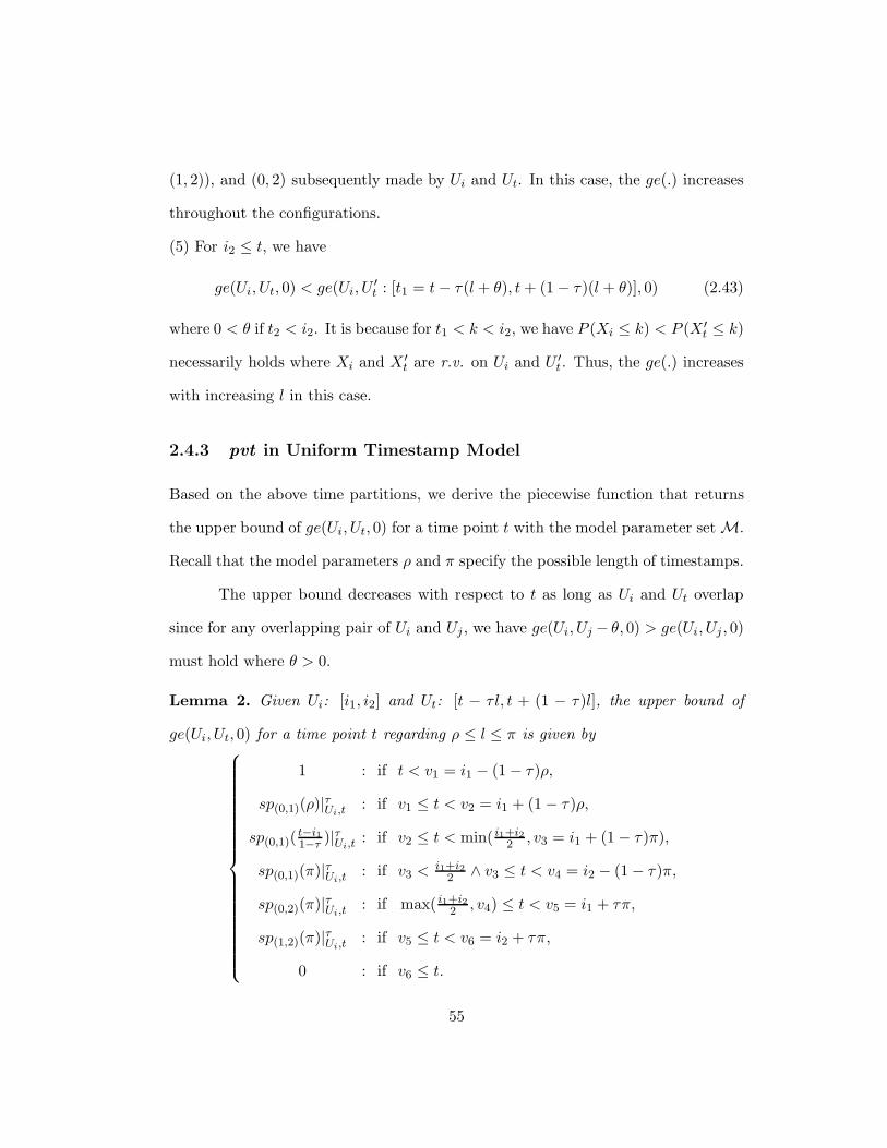
(1, 2)), and (0, 2) subsequently made by Ui and Ut. In this case, the ge(.) increases
throughout the configurations.
(5) For i2 ≤ t, we have
ge(Ui, Ut, 0) < ge(Ui, U′t : [t1 = t− τ(l + θ), t + (1− τ)(l + θ)], 0) (2.43)
where 0 < θ if t2 < i2. It is because for t1 < k < i2, we have P (Xi ≤ k) < P (X ′t ≤ k)
necessarily holds where Xi and X ′t are r.v. on Ui and U ′
t. Thus, the ge(.) increases
with increasing l in this case.
2.4.3 pvt in Uniform Timestamp Model
Based on the above time partitions, we derive the piecewise function that returns
the upper bound of ge(Ui, Ut, 0) for a time point t with the model parameter setM.
Recall that the model parameters ρ and π specify the possible length of timestamps.
The upper bound decreases with respect to t as long as Ui and Ut overlap
since for any overlapping pair of Ui and Uj , we have ge(Ui, Uj − θ, 0) > ge(Ui, Uj , 0)
must hold where θ > 0.
Lemma 2. Given Ui: [i1, i2] and Ut: [t − τ l, t + (1 − τ)l], the upper bound of
ge(Ui, Ut, 0) for a time point t regarding ρ ≤ l ≤ π is given by
1 : if t < v1 = i1 − (1− τ)ρ,
sp(0,1)(ρ)|τUi,t: if v1 ≤ t < v2 = i1 + (1− τ)ρ,
sp(0,1)(t−i11−τ
)|τUi,t: if v2 ≤ t < min( i1+i2
2 , v3 = i1 + (1− τ)π),
sp(0,1)(π)|τUi,t: if v3 < i1+i2
2 ∧ v3 ≤ t < v4 = i2 − (1− τ)π,
sp(0,2)(π)|τUi,t: if max( i1+i2
2 , v4) ≤ t < v5 = i1 + τπ,
sp(1,2)(π)|τUi,t: if v5 ≤ t < v6 = i2 + τπ,
0 : if v6 ≤ t.
55

Proof. Due to non-overlapping cases, obviously we have the first and the seventh
formulas. Here we sketch the proof of the other cases by using the timeline partitions
described in Chapter 2.4.2.
For v1 ≤ t < i1: by the partitioned case (1), we have the maximum of
ge(Ui, Ut, 0) when l is minimized (l = ρ).
For i1 ≤ t < i1+i22 : by the partition (2), we have the maximum of ge(Ui, Ut, 0)
when l = l′ = t−i11−τ
, if
ρ ≤ l′ ≤ π ⇒ v2 = i1 + (1− τ)ρ ≤ t ≤ v3 = i1 + (1− τ)π (2.44)
holds. Thus for v2 ≤ t < min( i1+i22 , v3), we have the maximum, sp(0,1)(l
′)|τUi,t. If
l′ < ρ, we have the maximum when l = ρ, since for l′ < t < i1+i22 , sp(0,1)(.) decreases
with respect to l. On the contrary, if π < l′, we have the maximum when l = π.
Combining these two cases v1 ≤ t < i1 and i1 ≤ t < i1+i22 above, we have
the third and the fourth formula. Notice that for any v1 < t < i1+i22 , there must be
such l value that makes the configuration (0, 1) (since 12 ≤ τ ≤ 1 and len(Ui) ≤ π).
For i1+i22 ≤ t: by the partitions (3)-(5), we have the maximum of ge(Ui, Ut, 0)
when l = π, as long as such l = π can make the configuration (0, 2). Since v4 =
i2− (1− τ)π ≤ t < v5 = i1 + τπ for the configuration (0, 2), we have the maximum,
sp(0,2)(π)|τUi,t, which corresponds to the fifth formula, for max( i1+i2
2 , v4) ≤ t < v5.
For v5 ≤ t < v6, we have only the configuration (1, 2) that can be made with
l = π, where ge(.) increases with respect to l, thus obtaining the sixth formula.
By taking the inverse function form regarding a confidence threshold δ from
the above upper bound function, we can establish the pvt(.) function for the uniform
model.
56

Theorem 7 (Uniform pvt). The probabilistic violation time, pvt(Ui)|Mpc in Defi-
nition 4 can be calculated in the uniform model as follows.
For 12 ≤ τ < 1, pvt(Ui)|Mpc =
i1 +√
2ρ(i1 − i2)(δ − 1) + ρ(τ − 1) + d : if p1 = sp(0,1)(ρ)|τUi,v2≤ δ < 1,
i1+i2+i1δ−i2δ−2i1τ2−2τ
+ d : if p2 = sp(0,1)(t′−i11−τ
)|τUi,t′≤ δ < p1,
i1 +√
2π(i1 − i2)(δ − 1) + π(τ − 1) + d : if v3 < i1+i22 ∧ p′2 = sp(0,1)(π)|τUi,v4
≤ δ < p2,
i1+i2+2π(τ−δ)2 + d : if p3 = sp(0,2)(π)|τUi,v5
≤ δ < p′,
i2 −√
2δπ(i2 − i1) + πτ + d : if 0 < δ < p3
where v2 ∼ v5 are given in Lemma 2, t′ = min( i1+i22 , v3), and p′ = p′2 if v3 < i1+i2
2 ;
otherwise, p′ = p2. For τ = 1, the first three formulas above are combined into
i1 +√
2π(i1 − i2)(δ − 1) + π(τ − 1) + d : if p′2 = sp(0,1)(π)|τUi,v4≤ δ < 1.
Proof. By taking the inverse function of the second formula in Lemma 2, that is,
by rearranging the formula using t′ such that sp(0,1)(ρ)|τUi,t′= δ, we have the first
formula in this theorem. The valid range of δ is calculated using the range values of
the corresponding second case in the lemma. The other formulas are found in the
same way.
2.5 Realizing the Potential of Monitoring Uncertain Event
Streams
The issue of temporal uncertainty is a common and challenging problem in many
embedded applications. Temporal uncertainty comes from the inherent restrictions
in the underlying sensing layer, such as the temporal/spatial limitations of sam-
pling, inaccurate clocks and unpredictable network latency. Although events occur
57

instantaneously (dense time) in the physical world, event occurrence often cannot be
assigned a precise time owing to the above limitations. Not surprisingly, a central-
ized processing architecture for correlating event streams from remote data sources
does not alleviate such the uncertainty in event timestamps.
While the physical system properties depend on event occurrence times, event
processing acts on event detection and notification time values. We have shown
that given a probability model of the temporal distance from event occurrence to
event detection, timing constraints based on event occurrence can be transformed
to those based on event detection. This transformation enables the early detection
of timing constraint violations. Let us illustrate this with an example. Consider a
campus surveillance system that tracks the locations of professors in real time by
taking images periodically of the faculty parking lot. Consider a punctual professor
who usually walks to his office from the parking lot within 3 minutes of arriving
at the parking lot. The professor has a student who will immediately launch a
search if the professor is late in showing up at his office. In this case, the safety
assertion for the professor not to become missing may be represented by a timing
constraint that defines a temporal relationship over a pair of events. We say that
the events at parking lot and at office occur when the professor enters respectively
the parking lot and his office. The safety assertion that the professor is not missing
can be expressed by a deadline timing constraint c that specifies an upper bound
of 3 minutes on the time interval between the at parking lot and at office events.
Suppose that one day the professor’s car is captured by a camera in the parking lot
at time 9:10 and later the professor logs-in the office computer at time 9:14. Here we
introduce some temporal uncertainty by assuming that the parking lot camera takes
58
pictures of the parking at one-minute intervals and that the professor logs in on his
computer at most within 2 minutes after he enters his office. Accordingly, we may
represent the timestamps of the corresponding at parking lot and at office events
respectively by the time intervals I1 : [9 : 09, 9 : 10] and I2 : [9 : 12, 9 : 14]. We
may also specify probabilistically the distribution of the actual time of occurrence
of the two events in the respective intervals. Let us use X1 and X2 to denote r.v.
on I1 and I2. If we assume a uniform distribution, we can compute the satisfaction
probability of the timing constraint c, P (X1 + 3 ≥ X2) = 0.25. The detection of
a probable timing constraint violation presupposes a confidence threshold in the
satisfaction probability of the constraint. With respect to a confidence threshold, it
is possible to calculate a violation detection time after which the constraint cannot
be met with a probability no lower than the threshold. We have shown how this
can be done efficiently by pre-computing a function of the maximum satisfaction
probability with respect to time and the uncertainty model of the timestamp. In
the above example, consider a probabilistic constraint pc : (c, 0.75) where 0.75 is the
threshold. In this case, the violation detection time is t = 9 : 13 for the constraint
pc, since P (X1 + 3 ≥ [t − 2, t]) = 0.75 and P (X1 + 3 ≥ [t + θ − 2, t + θ]) < 0.75
necessarily holds for any θ > 0. Hence, the violation of pc can be declared unless pc
is satisfied by time 9:13.
Given that the sensor has detected an event, the probability distribution
characterizes the uncertainty in the exact time of event occurrence as allowed by
the sensor. In general, the mathematical derivation of the violation detection time
formulae is dependent on the probability distribution specific to the sensor; Ptmon
in this chapter provides a customizable solution. In the following, we discuss how
59

ÒÓÔÔ ÒÕÖ× ÒØÙÚÛÜÝ Þ ÛÜÝ ß àáâãàáâãäàåâæ çèéãêàåáèàë àêåèäâáääáìè çèéãêàåáèàë
Figure 2.6: Event occurrence, detection, and arrival times
we can exploit the monitoring technique of Ptmon for real-world applications. In
particular, we discuss complications where the uncertainty related to detecting,
timestamping and transmitting events together renders the realization of general
monitoring functions problematic.
Figure 2.6 depicts the relationship of event occurrence, detection, and ar-
rival times. An event occurring at tocc, is detected/timestamped at tdet, and then
a notification is sent to a monitoring processor that receives it at time tarv. As
we have discussed earlier, imperfect sensing (such as sampling error) and other in-
frastructure limitations (such as clock synchronization) may render the accuracy of
detection less than 100% reliable. Thus, the timestamp of an event is an estimate
of tocc. In practice, a pdf may be acquired by understanding the statistical prop-
erties of the sensing and timestamping operations, the distribution on the interval
tdet − tocc via experiments. Similarly, the event transmission delay tarv − tdet may
not be deterministically given but its distribution may be obtainable empirically. In
addressing the problem of timestamp uncertainty, it is possible to simplify the prob-
lem of event transmission delays by relying on the event buffering method with the
assumption that the upper bound of the delay is known. This approach is justified
when the uncertainty of event transmission delays is relatively negligible, compared
to that of event timestamps.
60

Data sources in embedded applications (i.e., sensors) are normally located
in remote field locations but monitoring applications often run on in host server.
Yet many sensor networks cannot provide reliable guarantees on transmission de-
lays, except certain real-time networks such as fieldbus in industrial process control.
Furthermore, event transmission delays may have to include more than the latency
of underlying networks, e.g., polling intervals in case that the monitoring processor
periodically polls data sources to retrieve events of interest. For monitoring timing
constraints that define the temporal relationship of event occurrences, event buffer-
ing is commonly used to ensure that events remotely generated are processed in
their temporal order, and the expiration of a timer catching the violation of timing
constraints is delayed until the monitoring processor has completed the processing
of all the events that are detected up to the timer’s expiration. Whereas event
buffering is necessary for detecting timing constraint violations that are conditioned
on the non-occurrence of certain events, this implementation technique incurs addi-
tional delay in processing events, thus leaving less time to recover from the detected
constraint violations. In our previous example, suppose that it takes no more than
∆ time to deliver the events, e.g., the professor’s login record is periodically updated
to the monitoring host. Then, the violation of pc could not have been ascertained
before time 9 : 13 + ∆. In such situations, a customer might want to have more
fine-grained control on the responsiveness of the event monitor so as to provide flexi-
bility in scheduling reactions to the events. This could be achieved in a probabilistic
framework, similar to what we have done for addressing the timestamp uncertainty.
Rather than conservatively taking the upper bound of the delays, we could calculate
the minimum duration required for ascertaining constraint violations according to
61

a user-specific tolerance on false positives in constraint violation detection.
Here we discuss three real-life applications that can benefit from the frame-
work [60]: real-time baggage tracking, Internet applications, and wireless process
control.
Real-time baggage tracking. RFID technology and sensor networks are paving
a way to efficiently, economically track physical objects in various business domains.
The use of RFID technology for baggage tracking systems in airports is one exam-
ple. While the traditional baggage tracking systems in use today are limited in
their tracking range in that they can neither update the location of a passenger’s
bag continually nor access it quickly, RFID-enabled baggage tracking systems make
it possible to easily locate a passenger’s bag, thus providing the better tracking vis-
ibility, and eventually lowering the number of mishandled bags and the operational
cost. Event timing monitors can be used in RFID-enabled baggage tracking systems
as follows. Here the location update operations of a passenger’s bag by RFID tag
readings are the events of interest. Once a passenger’s bag is checked in, the latest
time for it to be on the plane is looked up. Then, for each RFID reader along the
path of the bag, the latest time by which the bag must be spotted passing by the
corresponding RFID reader is calculated. If any of the RFID events that detect
the bag does not occur in time, an alarm will be triggered. In order to realize this
tracking functionality, however, we must carefully address the temporal uncertainty
that comprises the inaccuracy from today’s error-prone RFID technology and the
variable delays caused not only by the transmission of raw RFID readings to the
central control system but by the processing required to transform the raw data into
62

meaningful application data through several data cleaning steps.
Internet applications. Net neutrality means no special treatment for any packet.
With many packets competing for routing resources on the Internet at any given
time, the network delay for a stream of data is highly variable and randomly dis-
tributed. It seems hopeless to bring real-time guarantees into the equation. How-
ever, probabilistic event monitoring could help in this direction. Given empirically
studied probabilistic models on network delays, event timing monitors such as Pt-
mon can be applied to Internet-based applications e.g., remote monitoring, online
multimedia downloading, teleconference, etc. For example, we can monitor the syn-
chronization of video and audio streams at the receiving end or monitor different
data packets within the same media stream. In doing so, the distribution function
for network delays can be used to calculate the pattern of out-of-order packets and
derive appropriate monitoring constraints.
Wireless process control. In industrial process control systems, both process
data and control data are generated and acted upon deterministically, usually pe-
riodically as well. The goal of this design, of course, is to minimize or eliminate
unpredictability. Put differently, unlike our interest in uncertainty, if the event
timestamp is not precise or not transmitted deterministically, the system configu-
ration is considered not properly working and so needs to be improved. For this
reason, typically real-time networks such as fieldbus are used. Meanwhile, the bene-
fit of wireless technology brings wireless network into the process control field. While
initially we only see wireless for non-critical part of the plant control, it is inevitable
63

Host Router
Router
Sensor Sensor
Actuator
Gateway
Figure 2.7: Wireless mesh network for process control
that process control over wireless, as depicted in Figure 2.7, will be required [55].
The inherent unreliability of wireless gives us new challenges. And the probabilistic
nature of transmission delays between two wireless nodes provides an appropriate
field to apply our study.
None of the current wireless standards or systems fits exactly the process
control requirements. Under the auspices of the ISA (Instrumentation, Systems,
and Automation Society), work is progressing in drafting new wireless standards for
this industry. It is reasonable that synchronization and multi-path will be included
in any new standards. Synchronization enables precise timestamping of sensor data.
To address the problem of wireless over process control, we need multi-path to
guarantee data delivery; but it also leads to variable data transmission delays. Jitter
in data transmission already exists and is manageable in non-wireless process control.
When it becomes significant in wireless process control, however, new techniques for
tackling it must be developed. One benefit of wireless for process control is that
more data can be collected and more aspects of process control become possible.
Correlations of different data streams could be formulated into timing constraints.
64

For example, a jump in upstream pressure will be reflected in a jump in downstream
pressure. What we have at the controller are a set of streaming data coming from
the wireless sensors. While the data is timestamped, the controller will receive
them with variable delays. The controller can check the timing constraints using
the probabilistic monitoring technique of Ptmon.
2.6 Summary
In this chapter, we have addressed the issue of temporal uncertainty in monitoring
timing constraints over events. Our approach is innovative in that it incorporates
the uncertainty of the difference between event occurrences and detections and it
provides a general framework for expediting the detection of timing constraint vio-
lations under the given different probabilistic models for the uncertainty.
In order to demonstrate the power of our framework, we have showed how
to derive the monitoring functionalities within the framework for gaussian, uniform,
and histogram distributions. As has been shown in Chapter 2.1, the framework
works as the timestamp-model-independent architectural layer for the monitoring
problem. To incorporate some other distributions (e.g., besides gaussian, histogram,
and uniform) in the framework, therefore, the appropriate implementation of the
functions ge, pvt and pvw is only needed. Note that the framework can be extended
by integrating a control mechanism for the degree of event timing uncertainty so
as to gain the flexibility between resource usages and event accuracy. For example,
given some latency requirement of a monitoring system, sensing and communication
by a set of wireless sensor devices can be enabled or disabled adaptively to trade
off resource consumption for the detection latency. When and how long a sensor or
65

communicator node is disabled will obviously impact the temporal uncertainty of
the sensor data stream.
66

Chapter 3
PTJOIN: Probabilistic Timing
Join
This chapter addresses the problem of processing event-timing join queries over
event streams where the uncertainty in the values of the timestamps is characteri-
zable by histograms. We describe a stream-partitioning technique for checking the
satisfaction of a probabilistic timing constraint upon event arrivals in a systematic
way in order to delimit the “probing range” in event streams. This technique can be
formalized as a probabilistic timing join Ptjoin operator where the join condition
is specified by a time window and a confidence threshold in our model. We present
efficient Ptjoin algorithms that tightly delimit the probing range and efficiently
invalidate events in event streams.
67

3.1 Event Timing Join
In this chapter, we show that the calculation of timing correlation can be cast into
the problem of performing a join operation that creates an output stream, where
each output tuple must satisfy the probability that the events in the join specification
occur together within a specified time interval. We refer to this class of band joins
over streams with temporal uncertainty as Ptjoin.
Example 7. Consider a set of sensor nodes that are spread densely in a surveillance
region where the detection latency of a suspicious activity by an intruder in the
region is probabilistically known according to specific sensor settings (i.e., sensing
modalities, power level, hardware mechanisms) and environmental conditions (i.e.,
variations on terrain and weather) via experiments [3]. To make a more accurate
hypothesis on possible intrusions, events from different modalities and nearby sensor
nodes can be joined based on their temporal proximity, that is, “if the probability that
acoustic and seismic sensor events occur within, say, 2000ms exceeds the confidence
threshold 0.6, then raise alarm for possible intrusion.” To adjust the false alarm
rate, this threshold must be updated efficiently.
The above example specifies a join calculation that is predicated on tempo-
ral proximity. A confidence threshold is embedded in a join condition to denote
the uncertainty of the temporal correlation. A SQL-style query representation for
Example 7 takes the following form:
select * from SEISMIC A, ACOUSTIC B
where WINDOW(A, B) = 2000 with THRESHOLD 0.6
The join condition of Ptjoin above is specified by two parameters, the time window
d = 2000 and the confidence threshold δ = 0.6. In general, we shall denote such a
68

join condition by jc: (d, δ); event ai in stream A and event bj in stream B qualify
jc iff P (Xi + d ≥ Xj ∧Xj + d ≥ Xi) ≥ δ holds where Xi and Xj are r.v. associated
with ai.ts and bj.ts respectively. Note that the case of using a uniform distribution
over time intervals has been studied in interval timing join [36]. For providing a
more generalized and flexible expression, we use the histogram timestamp model
introduced in Chapter 2.3.1.
A straightforward method to perform Ptjoin is as follows. Upon a new event
arrival in stream A (or B), first retrieve all events in stream B (or A) and then keep
evaluating the join condition with each of the possible event pairs. The evaluation
of the join condition may require performing the task of histogram adjustment to
check the temporal relationship between two events. Three problems arise with this
approach. First, how can we tightly delimit the set of event pairs being probed
upon an event arrival? Second, how can we efficiently evaluate the join condition
for an event pair? Third, how can we effectively manage stream buffers? Based on
the nested loop join model for sliding time windows [31], we investigate the stream
partitioning technique that tightly identifies the probing range for an arriving event
by parameterizing the uncertain temporal properties of streams and keeping events
in the temporal order. In particular, we show for an event arrival, how to partition
a temporally ordered event stream by finding minimum/maximum time points that
satisfy timing constraints associated to a join condition in a systematic way so
that we can optimize Ptjoin calculation with the necessary probing range. It
is possible to keep such a temporal order in streams without incurring significant
overheads owing to the fact that events normally arrive in ascending order of their
occurrence times [56]. The partitioning allows us to prune unnecessary join tests
69

and furthermore derive the tightest sliding time window over a stream, rendering
the events outside the sliding time window obsolete.
As described in Chapter 2.1.1, we consider only streams where the temporal
uncertainty of all the events can be bounded and specified by their model parameters.
It is because without the specification by the model parameters (in Definition 8), we
cannot confine the probing range to within a finite interval. Note that for specifying
the properties of multiple streams being involved in join operations, we especially
notate a model parameter m for stream A by mA , e.g., HA for the template his-
togram set of stream A. In addition to the model parameters previously given in
Definition 8 for the histogram model, we use the following parameter, similarly to
Definition 10 (2) of the uniform model.
Definition 11 (max length of timestamps). πA is a model parameter that de-
notes the maximum length of template histograms that can occur in stream A, i.e.,
∀φi ∈ HA, len(φi) ≤ πA holds.
In the following, we restrict our discussion to the cases where (1) the model
parameters in Definition 8 and 11 are known a priori as part of system specification,
and (2) the time window size d in Ptjoin queries is relatively large such that
d ≥ max(πA, πB) holds.1 In particular, with such d values, the evaluation of the
join condition jc in Ptjoin transforms to that of its associated probabilistic timing
constraint: (ai.ts+d ≥ bj .ts, δ) or (bj .ts+d ≥ ai.ts, δ) for a pair of events ai and bj .
Notice that we can check a probabilistic timing constraint such as (ai.ts+d ≥ bj .ts, δ)
by calculating ge(Hi,Hj, d) as explained in Chapter 2.3.
1Note that π used in Chapter 2.4 has the same meaning of the maximum length for uniformtimestamps, but in this chapter we use this symbol for the histogram model.
70
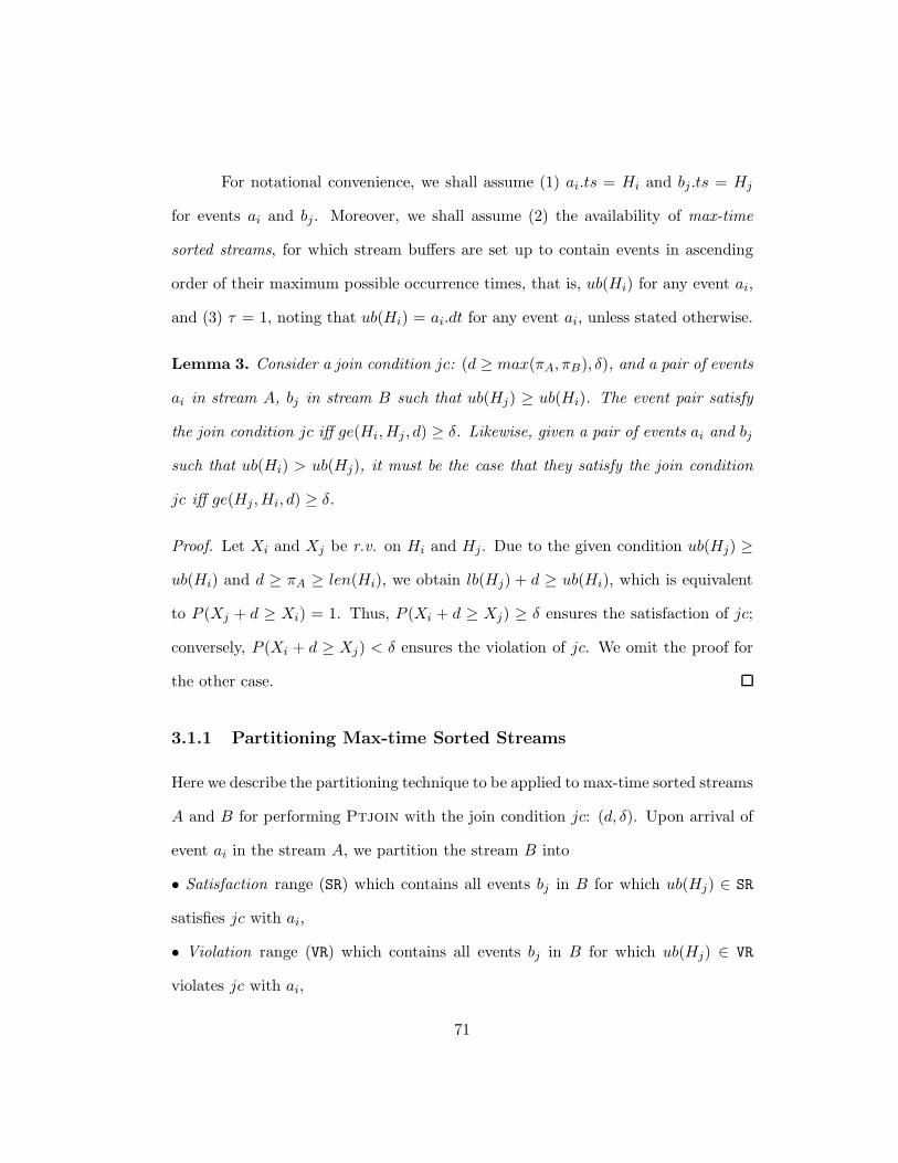
For notational convenience, we shall assume (1) ai.ts = Hi and bj.ts = Hj
for events ai and bj . Moreover, we shall assume (2) the availability of max-time
sorted streams, for which stream buffers are set up to contain events in ascending
order of their maximum possible occurrence times, that is, ub(Hi) for any event ai,
and (3) τ = 1, noting that ub(Hi) = ai.dt for any event ai, unless stated otherwise.
Lemma 3. Consider a join condition jc: (d ≥ max(πA, πB), δ), and a pair of events
ai in stream A, bj in stream B such that ub(Hj) ≥ ub(Hi). The event pair satisfy
the join condition jc iff ge(Hi,Hj , d) ≥ δ. Likewise, given a pair of events ai and bj
such that ub(Hi) > ub(Hj), it must be the case that they satisfy the join condition
jc iff ge(Hj ,Hi, d) ≥ δ.
Proof. Let Xi and Xj be r.v. on Hi and Hj. Due to the given condition ub(Hj) ≥
ub(Hi) and d ≥ πA ≥ len(Hi), we obtain lb(Hj) + d ≥ ub(Hi), which is equivalent
to P (Xj + d ≥ Xi) = 1. Thus, P (Xi + d ≥ Xj) ≥ δ ensures the satisfaction of jc;
conversely, P (Xi + d ≥ Xj) < δ ensures the violation of jc. We omit the proof for
the other case.
3.1.1 Partitioning Max-time Sorted Streams
Here we describe the partitioning technique to be applied to max-time sorted streams
A and B for performing Ptjoin with the join condition jc: (d, δ). Upon arrival of
event ai in the stream A, we partition the stream B into
• Satisfaction range (SR) which contains all events bj in B for which ub(Hj) ∈ SR
satisfies jc with ai,
• Violation range (VR) which contains all events bj in B for which ub(Hj) ∈ VR
violates jc with ai,
71

• Probing range (PR) which contains all events bj in B for which ub(Hj) ∈ PR may
or may not satisfy jc with ai.
With these partitions, we can limit probing events in B to only those in PR. Regard-
less of the value of δ, we can have the partitions constructed by two PRs:
LPR = [lb(Hi)− d, ub(Hi)− d + πB), RPR = (lb(Hi) + d, ub(Hi) + d + πB] (3.1)
Therefore, only events bj such that ub(Hj) ∈ LPR or ub(Hj) ∈ RPR in B will be
checked with ai. Not surprisingly,
SR = [ub(Hi)− d + πB, lb(Hi) + d] (3.2)
is surrounded by two PRs, and VR is necessarily confined by the ranges that are
neither PRs nor SR. Given a specific confidence threshold δ, we can find the tightest
PRs for an event that triggers the probing over a stream of its join partners.
Theorem 8 (stream partitions). Consider jc: (d ≥ max(πA, πB), δ). Upon
arrival of event ai such that Hi ≃ φu in stream A, we have the partitions in stream
B as follows:
LPR = [ minφv∈HB
ht(φu, φv , 1− δ) + g(−d), maxφv∈HB
ht(φu, φv, 1− δ) + g(−d)),
RPR = ( minφv∈HB
ht(φu, φv, δ) + g(d), maxφv∈HB
ht(φu, φv , δ) + g(d)]
where g(x) = ub(Hi)− ub(φu) + x. Note that ht(.) function is in Equation 2.19.
Proof. Let us denote two time points of RPR by rpr1 = minφv∈HBht(φu, φv, δ) +
g(−d) and rpr2 = maxφv∈HBht(φu, φv , δ) + g(−d). Consider an event br ≃ φk
(φk ∈ HB) such that ub(Hr) > rpr2 and ub(Hr) ≥ ub(Hi) hold. And further let
tk = ht(φu, φk, δ)+ub(Hi)−ub(φu)+d. By Theorem 8, then, we conclude that since
72
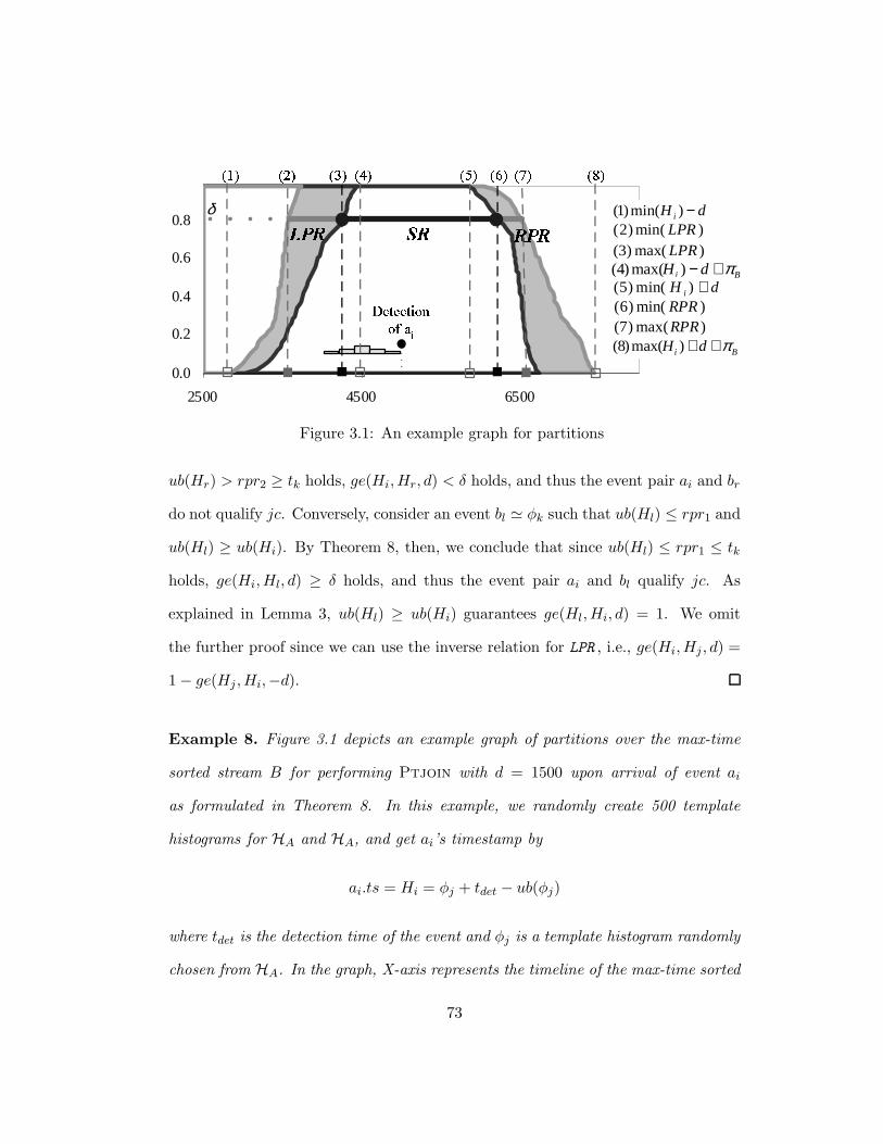
2500 4500 6500
0.0
0.2
0.4
0.6
0.8δ íîïðî îðîñòóòôóõö÷öø ùú
ûüý ûþý ûÿý û�ý û�ý û�ý û�ý û�ýBi dH π+−)max()4(
)max()3( LPR
dH i −)min()1()min()2( LPR
)max()7( RPR
Bi dH π++)max()8(
dH i +)min()5()min()6( RPR
Figure 3.1: An example graph for partitions
ub(Hr) > rpr2 ≥ tk holds, ge(Hi,Hr, d) < δ holds, and thus the event pair ai and br
do not qualify jc. Conversely, consider an event bl ≃ φk such that ub(Hl) ≤ rpr1 and
ub(Hl) ≥ ub(Hi). By Theorem 8, then, we conclude that since ub(Hl) ≤ rpr1 ≤ tk
holds, ge(Hi,Hl, d) ≥ δ holds, and thus the event pair ai and bl qualify jc. As
explained in Lemma 3, ub(Hl) ≥ ub(Hi) guarantees ge(Hl,Hi, d) = 1. We omit
the further proof since we can use the inverse relation for LPR , i.e., ge(Hi,Hj , d) =
1− ge(Hj ,Hi,−d).
Example 8. Figure 3.1 depicts an example graph of partitions over the max-time
sorted stream B for performing Ptjoin with d = 1500 upon arrival of event ai
as formulated in Theorem 8. In this example, we randomly create 500 template
histograms for HA and HA, and get ai’s timestamp by
ai.ts = Hi = φj + tdet − ub(φj)
where tdet is the detection time of the event and φj is a template histogram randomly
chosen from HA. In the graph, X-axis represents the timeline of the max-time sorted
73

stream B in milliseconds and Y-axis represents the probability. The figure clearly
shows two PRs and SR when δ = 0.8 and tdet = 5000, highlighting their tightness
with the comparison of those by Equation 3.1 and 3.2. The time points (2), (3), (6)
and (7) represent the partitions by Theorem 8 while the time points (1), (4), (5) and
(8) represent the partitions by Equation 3.1 and 3.2.
Lemma 3 and Theorem 5 provide a join method that evaluates the Ptjoin
condition for an event pair in the probing ranges, using their respective template
histograms. Consider events ai and bj such that Hi ≃ φu and Hj ≃ φv. If ub(Hj) ≥
ub(Hi) holds, we can check if the inequality
ht(φu, φv , δ) + d + ub(Hi)− ub(φu) ≥ ub(Hj) (3.3)
for evaluating the probabilistic timing constraint (Hi + d ≥ Hj , δ); otherwise, we
can check if the inequality
ht(φu, φv, 1 − δ) − d + ub(Hi)− ub(φu) ≤ ub(Hj) (3.4)
holds for evaluating the probabilistic timing constraint (Hj +d ≥ Hi, δ). Notice that
such ht(.) for specific δ and 1− δ values can be pre-computed for a set of template
histograms at query installation time, and thus evaluating the join condition for an
event pair in PRs can be done in constant time.
3.1.2 Managing Stream Buffers
Whereas most conventional sliding window joins include an explicit clause for the
time window in their join specification and rely on event buffering for dealing with
any possibly delayed event arrivals, we need to derive the sliding time window from
the Ptjoin condition and the stream parameters. Since Theorem 8 restricts the
74

candidate join partners for an arriving event within a combined time window of SR
and PR, it is possible to find the maximum time point for removing obsolete events
that will not become a join partner of any future event. Clearly, such maximum
time point confines the sliding time window over a stream.
Theorem 9 (obsolete event condition). Consider jc: (d ≥ max(πA, πB), δ).
When the join operation triggered by event ai in stream A is processed, any event bj
in a stream B such that ub(Hj) < ub(Hi)−DA−d+tmin must be obsolete where tmin
= minφu∈HA,φv∈HBht(φu, φv, 1− δ)− ub(φu). Note that DA is the model parameter
for the transmission delay of an event (in Definition 8).
Proof. According to Definition 8, when processing event ai in A, we may have the
maximum possibly delayed event aj in A such that ub(Hj) = ub(Hi)−DA. Assuming
such an event aj ≃ φk, consider time tl = minφv∈HBht(φk, φv, 1 − δ) + max(Hi)−
ub(φk) − d as similarly shown in Theorem 8. Any event whose max time is earlier
than tl cannot be a join partner of aj due to the property of PRs. The minimum
possible tl by all possible template histograms φu ∈ HA guarantees that any possible
pair of aj in A and bl in B such that ub(Hl) < tl must violate the join condition.
A stream buffer can be implemented as a circular buffer such that front and
rear pointers are maintained to locate the valid sliding time window over a max-time
sorted stream. A stream buffer grows as a new event is placed at the rear position,
but it shrinks as obsolete events are removed by advancing the front pointer. Based
on Theorem 9, the sliding time window over a stream for Ptjoin can be tightly
constructed whenever a new arriving event is processed and inserted into a stream
buffer by setting the front pointer to just after the latest obsolete event. Notice that
75
the time offset to the latest obsolete events is a constant that can be calculated at
query installation time regarding all possible template histogram pairs. It should be
noted that the model parameter for denoting the maximum possible network delays,
i.e., DA is needed to ensure that the invalidated events cannot be joined even if some
event triggering the join operation may arrive late within the parameter value.
3.1.3 Handling Unknown Templates
Thus far, we have shown that if template histograms are known, PR can be com-
puted by identifying a pair of template histograms that have the minimum and the
maximum satisfaction time for each template histogram at query installation time.
Here we consider the removal of the previous assumption that a set of template
histograms, e.g., HA for a stream A are known a priori. We consider the particular
case where the probability distribution on the detection latency of events is dynami-
cally determined depending on various environmental settings as in Example 7. For
this case, we assume the stream parameters in Definition 11 are given without the
specification of individual template histograms.
In the absence of template histograms, upon arrival of event ai in a stream
A, we have the partitions for a stream B as follows:
LPR = [tδ − d, tδ − d + πB), RPR = (t1−δ + d, t1−δ + d + πB ] (3.5)
where tδ is a time point such that P (Xi ≤ tδ) = δ and t1−δ is a time point such that
P (Xi ≤ t1−δ) = 1− δ. Here, we can find the time offset for keeping the sliding time
window: when the join operation triggered by ai in a stream A is processed, we can
conclude that any event bj in a stream B such that ub(Hj) < ub(Hi)−DA− d−πA
must be obsolete, thereby obtaining the time offset, DA + d + πA.
76

����� � �� �� � ������������� �����
���
����� � �� �� � �����
�!"#"$ %&'
Figure 3.2: Updating the bounds of ge(Hi,Hj, 0)
For evaluating the join condition of a event pair in PRs, we need to evaluate its
associated timing constraint at runtime. Given ge(Hi,Hj, d) ≥ δ, obviously we can
determine its satisfaction or violation by considering the adjusted histograms H ′i and
Hj of H ′i = Hi+d and Hj and then evaluating calGe(H ′
i, Hj) (in Algorithm 3). With
a specific confidence threshold δ, however, it is only necessary to know whether the
satisfaction probability exceeds it or not, so we can efficiently check the constraint
during the task of histogram adjustment by updating the bounds of its satisfaction
probability and comparing them with the threshold for early termination. For sim-
plicity, we omit d in the following illustration since Hi + d is a shifted histogram of
77

Hi by d,
Let sp = ge(Hi,Hj , 0), and Xi, Xj be r.v. for Hi and Hj respectively. The
probability that one histogram definitely precedes or succeeds the other can be used
to approximate the bounds of sp before performing histogram adjustment. For
example, given the histogram pair in Figure 3.2(a), we establish the initial bounds
from the non-overlapping buckets,
P (Xi ≥ tr) + P (Xj ≤ tl)− P (Xi ≥ tr)P (Xj ≤ tl) < sp < 1 (3.6)
where tr = ub(Iiu) such that ub(Hj) ∈ Iiu and tl = lb(Ijv) such that lb(Hi) ∈ Ijv. If
these bounds are not tight enough, we can start histogram adjustment only with the
overlapping buckets (gray buckets in Figure 3.2(a)). For each shared subinterval Is
(dark buckets in Figure 3.2(b)) that is identified during histogram adjustment, we
update the bounds of sp by adding the gain probability of Is to the current lower
bound and subtracting the loss probability of Is from the current upper bound. The
gain probability is calculated by
P (Xi ∈ Is)P (tl ≤ Xj ≤ lb(Is)) +P (Xi ∈ Is)P (Xj ∈ Is)
2(3.7)
and the loss probability is calculated by
P (Xi ∈ Is)P (Xj ≥ ub(Is)) +P (Xi ∈ Is)P (Xj ∈ Is)
2. (3.8)
3.2 Evaluation
To evaluate the effectiveness of our approach, we have implemented an event stream
monitor as our testbed to conduct performance experiments. As illustrated in Fig-
ure 3.3, the monitor includes three packages written in JDK 1.5: stream receiver,
78

()*+,- *+.+/0+*10+2).3**+4,)3*
56789: ;
()*+,- <=>>+* ? ()*+,- <=>>+* @A8B977CD9E
FGHIFGEEJ7KA6L897
M=)N=) O)*+,-CAH87678:KD8 7867C8D8J7KA6L897
PQ56789: R
QSQTSQU VWXYZ[ \] ^_` aδ
Figure 3.3: Event monitoring architecture for Ptjoin
stream buffer and event correlator. Through the receiver, an event is sent to the
correlator, processed according to the stream operator plugged-in, and stored in the
stream buffers for further processing by future events. Because of the lack of publicly
available benchmark for uncertain event streams, we implemented an event genera-
tor that can produce event streams with randomly created histograms that satisfy
given stream parameters. Each event contains stream id, sensor id, histogram, and
optional data attributes. All the experiments were run on a PC with a Pentium4
2.4GHz processor and 512M main memory against a data file which has 20k events,
with an exponential distribution on their inter-occurrence times. Stream buffers
were set up to keep the sorted-index over max time (ub(H)) of histograms.
Algorithm 4 encodes the framework for computing Ptjoin. Upon arrival of
event si, the join operation takes 5 steps: calculating the time windows for two PRs,
SR (line 2), evaluating the join condition with the events in PRs (line 5), outstreaming
79
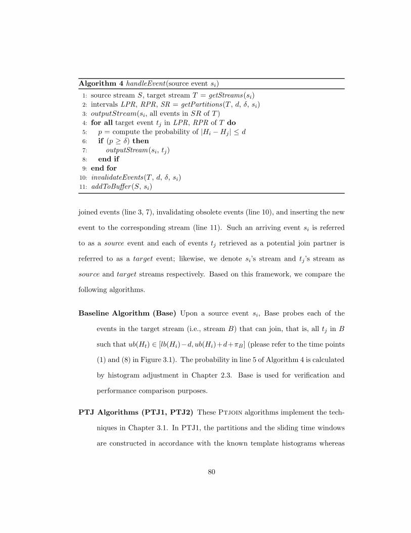
Algorithm 4 handleEvent(source event si)
1: source stream S, target stream T = getStreams(si)2: intervals LPR, RPR, SR = getPartitions(T , d, δ, si)3: outputStream(si, all events in SR of T )4: for all target event tj in LPR, RPR of T do5: p = compute the probability of |Hi −Hj| ≤ d6: if (p ≥ δ) then7: outputStream(si, tj)8: end if9: end for
10: invalidateEvents(T , d, δ, si)11: addToBuffer (S, si)
joined events (line 3, 7), invalidating obsolete events (line 10), and inserting the new
event to the corresponding stream (line 11). Such an arriving event si is referred
to as a source event and each of events tj retrieved as a potential join partner is
referred to as a target event; likewise, we denote si’s stream and tj’s stream as
source and target streams respectively. Based on this framework, we compare the
following algorithms.
Baseline Algorithm (Base) Upon a source event si, Base probes each of the
events in the target stream (i.e., stream B) that can join, that is, all tj in B
such that ub(Ht) ∈ [lb(Hi)−d, ub(Hi)+d+πB ] (please refer to the time points
(1) and (8) in Figure 3.1). The probability in line 5 of Algorithm 4 is calculated
by histogram adjustment in Chapter 2.3. Base is used for verification and
performance comparison purposes.
PTJ Algorithms (PTJ1, PTJ2) These Ptjoin algorithms implement the tech-
niques in Chapter 3.1. In PTJ1, the partitions and the sliding time windows
are constructed in accordance with the known template histograms whereas
80

the technique for checking a timing constraint at runtime for unknown tem-
plate histograms in Chapter 3.1.3 is mainly tested in PTJ2.
The performance metric we are interested in is the required time for Ptjoin
operations per event arrival, termed sid (stream-in delay):
sid =
∑
ctim(si)− atim(si)
N
where ctim(si) is the time when an event si is inserted into the stream buffer af-
ter completing the join operations by si, atim(si) is the time when an event si is
received, and N is the total number of processed events. Since the delay duration
may not be stabilized until stream buffers are sufficiently filled, only the perfor-
mance data after stabilization was considered. In this chapter, the time unit of the
time window d and sid is in milliseconds and λ denotes the event occurrence rate,
the average number of events per second. Table 3.1 illustrates the stream parameter
settings that were used to create event streams with different characteristics. The
stream parameters (defined in Chapter 3.1) are set identically for two streams, so
each stream name is omitted here. In the table, avg|H| denotes the average number
of buckets in histograms and |H| denotes the number of template histograms in a
stream. Three different test classes (small, med, large) were designed. Although
these settings were chosen in lieu of unavailable benchmarks, the following results
in terms of sid of the PTJ algorithms compared to that of the baseline algorithm
provide an assessment of our approach.
Here, let us consider the performance of Ptjoin, given a set of template
histograms as a stream parameter. The event generator was programmed to create
a set of template histograms and then event streams were created from the set of
81

small med large
avg|H| 5 10 20
π 500 1000 1500D 1000 1500 2000|H| 100 500 1000
Table 3.1: Stream parameter settings
template histograms according to the parameter settings in Table 3.1. Figure 3.4
shows the number of probings and joined tuples in Base and PTJ1 with various
confidence thresholds, δ. In this test, class=med, d=2000, and λ=100 are given,
and X-axis represents δ. In figure(a), Y-axis represents the number of joined tuples
(#join). In figure(b), Y-axis represents the number of probings by Base (#prb B),
the number of probings by PTJ1 (#prb P), the number of joined tuples in PRs by
PTJ1 (#jPR P), and the number of joined tuples in SR by PTJ1 (#jSR P). As
expected, with larger δ, the number of joined tuples decreases. Note that in PTJ1,
the number of probings slightly increases but the number of joined tuples in SR
decreases as δ increases. This result corresponds to the graph in Figure 3.1; with
larger δ, SR and RPR shrink, but LPR is extended instead. Likewise, Figure 3.5 shows
the number of probings and joined tuples with various time windows, d. In this test,
class=med, δ=0.8, and λ=100 are given and X-axis represents d. In figure(a), Y-axis
represents the number of joined tuples (#join). In figure(b), Y-axis represents the
number of probings by Base (#prb B), the number of probings by PTJ1 (#prb P),
the number of joined tuples in PRs by PTJ1 (#jPR P), and the number of joined
tuples in SR by PTJ1 (#jSR P).
The number of joined tuples increases along with larger d; interestingly, in
PTJ1, the number of joined tuples from SR increases but that from PRs does not. It
is because the size of PRs is independent of d.
82

0
2000000
4000000
6000000
0.1 0.2 0.3 0.4 0.5 0.6 0.7 0.8 0.9
#join
bcd0
2000000
4000000
6000000
0.1 0.2 0.3 0.4 0.5 0.6 0.7 0.8 0.9
#prb_B
#prb_P
#jRP_P
#jSR_P
bedFigure 3.4: The number of joined tuples and probings with various δ
Figure 3.6-3.7, under various thresholds and time windows, clearly show the
performance advantage of our partitioning scheme, that is, pre-calculating the satis-
faction time of template histogram pairs provides the offset time for constructing PRs
as well as for checking the join condition of an event pair. In Figure 3.6, class=med,
d=2000, and λ=100 are given; X-axis represents δ and Y-axis represents sid. Sim-
ilarly in Figure 3.7, class=med, δ=0.8, and λ=100 are given; X-axis represents d
and Y-axis represents sid. Particularly, sid of Base increases but that of PTJ1 are
stabilized as d increases. This highlights the benefit of the construction of SR, that
is, a larger d setting poses not larger PRs but a larger SR.
Figure 3.8-3.9 show the performance effect of various event occurrence rates
83

0
2000000
4000000
6000000
8000000
1500 2300 3100 3900
#join
fgh
0
2000000
4000000
6000000
8000000
10000000
1500 2300 3100 3900
#prb_B
#prb_P
#jRP_P
#jSR_P
fihFigure 3.5: The number of joined tuples and probings with various d (window size)
in streams. In Figure 3.8, class=med, d=1500 in (a), 3500 in (b), and δ=0.2,0.4,0.6,0.8
are given; X-axis represents 1000/λ and Y-axis represents sid of Base. Similarly in
Figure 3.9, class=med, d=1500 in (a), 3500 in (b), and δ=0.2,0.4,0.6,0.8 are given;
X-axis represents 1000/λ and Y-axis represents sid of PTJ1. Of course, the the
higher rates require more computation to perform the join operations for an event,
so sid is expected to increase as λ gets higher. Most importantly, the effect is rela-
tively less significant to PTJ1 because of its pre-calculation of satisfaction times.
Now let us consider the performance of Ptjoin when template histograms
are not available. In doing so, we compare Base and PTJ2 against randomly gen-
erated event streams without template histograms. Figure 3.10-3.11 illustrate the
84

0
1
2
3
0.1 0.3 0.5 0.7 0.9
BasePTJ1
c
Figure 3.6: Performance with various δ
0
1
2
3
1500 2300 3100 3900
BasePTJ1
Figure 3.7: Performance with various d (window size)
performance comparison of difference classes with various δ and λ. Clearly, PTJ2
outperforms Base in all the test cases. In Figure 3.10, d=1500 and λ=100 are given;
X-axis represents the class and δ, and Y-axis represents sid. Similarly in Figure 3.11,
d=1500 and δ=0.8 are given; X-axis represents the class and 1000/λ, and Y-axis
represents sid.
It should be noted that PTJ2 constructs the partitions less tightly due to the
absence of template histograms. However, PTJ2 can end the computation for a pair
of histogram timestamps before adjusting all of their buckets so as to reduce the
85

jkl mnoo
jpl qnoo0
2
4
6
8
10
20 18 16 14 12 10 8 6
0.2 0.4 0.6 0.8
0
2
4
6
8
10
20 18 16 14 12 10 8 6
0.2 0.4 0.6 0.8
Figure 3.8: Base with various λ (event rate)
probing cost. Since more buckets in histogram timestamps incur more computation
in checking timing constraints at runtime, sid of Base degrades with the large class.
It is observable that such degradation is quite insignificant for PTJ2.
3.3 Summary
In this chapter, we have addressed the issue of temporal uncertainty in processing
a continuous join query over event streams. We assume the uncertainty model such
that exact time of event occurrences may be known only probabilistically. With
86
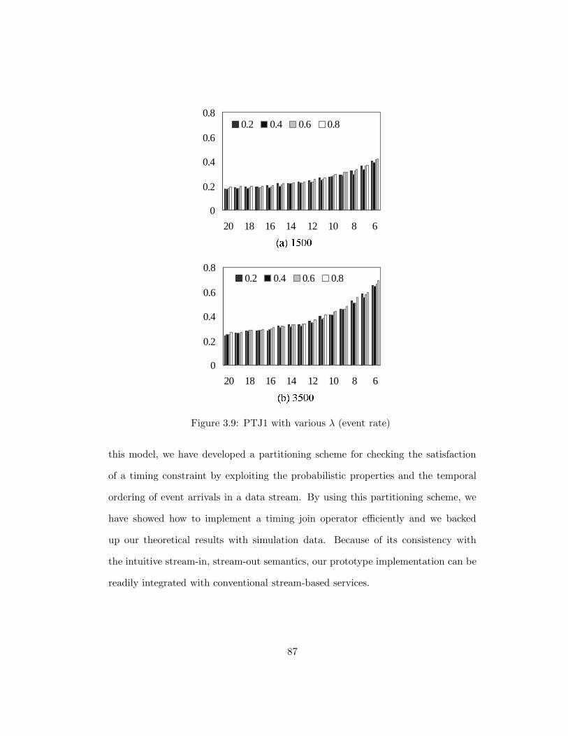
rst uvww
rxt yvww
0
0.2
0.4
0.6
0.8
20 18 16 14 12 10 8 6
0.2 0.4 0.6 0.8
0
0.2
0.4
0.6
0.8
20 18 16 14 12 10 8 6
0.2 0.4 0.6 0.8
Figure 3.9: PTJ1 with various λ (event rate)
this model, we have developed a partitioning scheme for checking the satisfaction
of a timing constraint by exploiting the probabilistic properties and the temporal
ordering of event arrivals in a data stream. By using this partitioning scheme, we
have showed how to implement a timing join operator efficiently and we backed
up our theoretical results with simulation data. Because of its consistency with
the intuitive stream-in, stream-out semantics, our prototype implementation can be
readily integrated with conventional stream-based services.
87
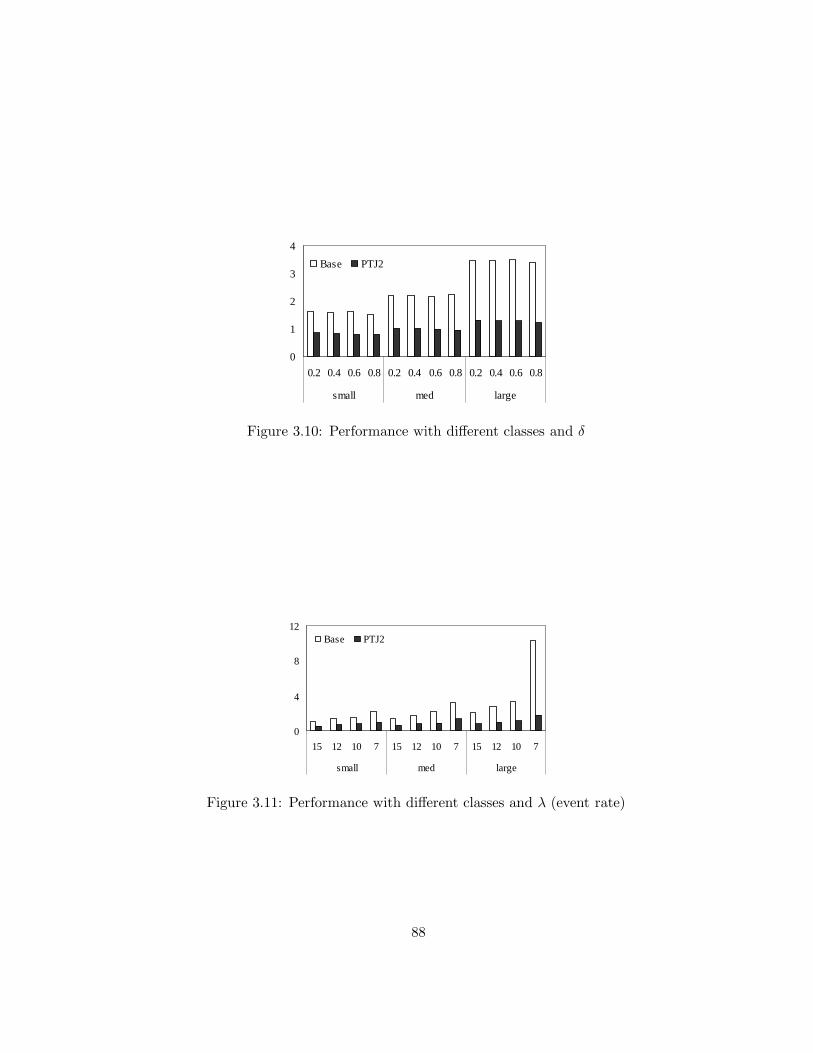
0
1
2
3
4
0.2 0.4 0.6 0.8 0.2 0.4 0.6 0.8 0.2 0.4 0.6 0.8
small med large
Base PTJ2
Figure 3.10: Performance with different classes and δ
0
4
8
12
15 12 10 7 15 12 10 7 15 12 10 7
small med large
Base PTJ2
Figure 3.11: Performance with different classes and λ (event rate)
88

Chapter 4
SPMON: Similarity-based
Probabilistic Monitoring
Data uncertainty is a common problem for the real-time monitoring of data streams.
In this chapter, we address the issue of efficiently monitoring the satisfaction/violation
of user-defined value-based constraints over data streams where the data uncertainty
can be probabilistically characterized. We propose a monitoring architecture Spmon
that can incorporate probabilistic models of uncertainty in constraint monitoring.
We adapt the concept of data similarity in real-time databases to the processing of
uncertain data streams. In doing so, we generalize the data similarity by a new con-
cept psr (probabilistic similarity region) that allows us to define similarity relations
for probabilistic data with respect to the set of constraints being monitored. This
enables the construction of lightweight filters for saving bandwidth. We also show
how to efficiently update the filter conditions at run-time.
89
4.1 Probabilistic Monitoring and Filtering
With the adoption of wireless technology in process control applications, the mini-
mization of communication between field devices and host systems is an important
issue because of the bandwidth and power limitations in the wireless devices. A
well-known strategy is for the resource-limited field devices to report sensor data to
the host system only if the data indicates critical state changes of the industrial pro-
cess under control that the host system must know about [7]. This type of strategy
has also been studied to guarantee QoS (quality of service) in the control-theoretic
setting [40, 41]. A simple example of this strategy is for a pressure sensor to report
its data to the host system if the pressure deviates from some range, say, [500, 1000]
psi. This simple rule is straightforward to implement if there is no uncertainty in
the sensor data. However, this is no longer the case if the sensor measurements are
known to have significant errors due to temporal and spatial uncertainties or other
physical limitations, as is the case of many wireless sensor monitoring systems.
For example, suppose a pressure sensor obtains a measurement of 990 psi but
the measurement can be off by 20 psi. Then the actual pressure can be as low as 970
psi and as high as 1010 psi. In this case it is easy to see that there is a 0.25 probability
that the actual pressure has exceeded 1000 psi, assuming that the error probability
is uniformly distributed over the [970, 1010] interval of possible pressure values. The
decision for the sensor to signal the host system or not can now depend on whether
the 0.25 probability is deemed acceptable for the application. For example, given a
user-specified threshold δ in probability, the monitoring condition can be specified
as: “whether or not the probability that the pressure is in between 500 and 1000 psi
is no smaller than δ.” Such probability threshold requirement is common for query
90

specification in the uncertain database literature [8, 10, 15].
In general, the processing of sensor data to determine whether or not the host
system needs to be signalled can be rather complex if a constraint specifying the
critical state change involves more than a single data stream, e.g., a join relation
involving pressure data from different locations in a pipe. This problem can be
alleviated by an architecture that combines “edge filters” and a “stream processor”
such that each data source (or a sensor node) can set up an edge filter to minimize the
transmission of data that does not cause some query result to change, and the stream
processor can recalibrate the edge filters. Here, we use the term filtering to denote
the suppression of unnecessary data transmission and redundant computation in the
context of monitoring continuous queries in stream data management. This differs
from the filtering in classical signal processing for noise reduction, which is not our
interest. This architecture of using edge filters has been studied in various areas
such as distributed web caches (e.g., TRAPP system [51]), moving object databases
(e.g., safe region based spatial query processing [52, 27]), and stream databases (e.g.,
adaptive filters [50, 9]). In [50], Olston et. al. investigated the filter adaptation for
monitoring continuous aggregation queries over distributed data sources where each
source tracks its exact numerical value and maintains an interval containing the
exact value as the filter condition. Employing edge filters is also consistent with
emerging industrial standards such as the WirelessHart standard for the process
control industry [26].
In this chapter, we address the problem of data uncertainty in monitoring
constraint-based queries in the stream database context and provide an efficient
solution for maintaining edge filters. While aiming at reducing the communication
91

load in a monitoring system like the related work above e.g., [50, 9], our problem is
distinct in two aspects that we (1) assume inherent uncertainty in underlying data
and (2) consider user-defined constraints with probability thresholds as continuous
query specification. Because of these two aspects, the condition of edge filters is
formulated based on the constraint specifications and dynamically set by the value
changes, and furthermore is made consistent with the uncertainty model. Therefore,
our problem is different from monitoring dynamic objects with static precision re-
quirements being individually imposed on the objects. Relating to the uncertainty,
we assume that data values at each data source are taken in discrete timesteps and
each data value is only given by a pdf.
The efficiency in our method makes explicit use of the concept of data space
similarity from our earlier work [34, 7]. Figure 4.1 illustrates the structure of Spmon.
The data sources (ds in the figure) rely on their edge filters (EFil) to determine if
new data values need to be forwarded to the stream processor which in turn updates
the filtering criteria of the edge filters and returns the evaluation results of monitored
constraints. Central to the operation of the edge filter is the concept of psr.
4.1.1 Uncertain Data Stream Model
The source of data is a set of real-valued objects O={oi}i=1,2,...,|O|. In generating
data values for the data sources, each object embodies a stochastic process that is
indexed by time. Throughout this chapter, we make the following assumptions.
(1) The value of an object is a function of time. The value can only be estimated
at every timestep by a pdf. A pdf is specified by its parameters as dictated by the
distribution type. For example, a gaussian pdf is defined by its (mean, standard
92

deviation) pair. We shall use the term p-data to denote the set of parameters that
characterize a pdf, and the term p-data space to denote the Cartesian space whose
coordinates are the parameters of the pdf.
(2) Each object generates a sequence of p-data as measured by the data sources
at each timestep. We use this stream structure independently of models for p-data
acquisition, which should be application-specific. The discussion about stochastic
modeling techniques for dynamic objects can be found in [15, 49, 30].
(3) The data sources are stateless. The p-data obtained by a sensor is dependent
solely on the true value of the object at the time of measurement and the device
characteristics of the sensor.
4.1.2 Value-based Constraints with Thresholds
Throughout this chapter, we consider value-based constraints of the following two
forms:
cR : r ≤ oi ≤ r, cJ : r ≤ oi − oj ≤ r (4.1)
where [r, r] is an interval such that r, r ∈ R and r < r. We refer to cR and cJ as
range constraint and join constraint respectively. Notice here oi and oj refer to the
true values of the objects that can only measured statistically by their p-data.
In Chapter 2, we have investigated the timing constraint monitoring over
uncertain event timestamps using a generalized probabilistic model-based approach.
Our work here is complementary to that in Chapter 2 in that we focus on the
monitoring of value-based constraints on uncertain data attributes of events.
Given p-data u of oi and v of oj in timestep t, the satisfaction probability of
93

cR and cJ are defined respectively as:
prob(cR)|u = P (r ≤ Xi ≤ r),
prob(cJ )|u,v = P (r ≤ Xi −Xj ≤ r)
where Xi and Xj denote respectively the r.v. associated with oi and oj in timestep
t. Notice that Xi and Xj are represented by their p-data.
We now define the probabilistic constraints for continuous query specification
as follows. A probabilistic constraint pc is a pair: (c, δ) where c is a constraint and
0 < δ < 1 is a confidence threshold in probability. Corresponding to the range
and join constraints, the probabilistic range and the probabilistic join constraint are
denoted by the pairs:
pcR : (cR, δ) and pcJ : (cJ , δ) (4.2)
A probabilistic range constraint is satisfied (we write: pcR|u = satisfaction) if its
satisfaction probability is not smaller than the given confidence threshold, and it is
violated (we write: pcR|u = violation) otherwise. Likewise, pcJ |u,v = satisfaction if
prob(cJ )|u,v ≥ δ. As described, we use c and pc for value-based constraints through-
out Chapter 4. There should be no confusion with those for timing constraints in
Chapter 2.
Example 9. Consider a set of probabilistic constraints: pc1:(0 ≤ o1 ≤ 60, 0.2),
pc2:(−20 ≤ o1 ≤ 75, 0.6), pc3:(−40 ≤ o1 − o2 ≤ 20, 0.4). And suppose p-data u and
v are generated for o1 and o2 respectively in timestep t1, and given by gaussian
distribution, e.g., u ∼ N(58, 102) and v ∼ N(79, 22). Then we have prob(0 ≤
o1 ≤ 60)|u = 0.58, prob(−20 ≤ o2 ≤ 75)|v = 0.02, prob(−40 ≤ o1 − o2 ≤ 20)|u,v = 0.97
94
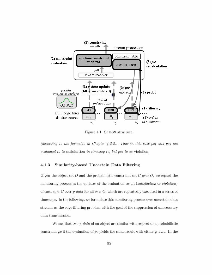
z{| }~���� ������z������ �����������|��������� ����� ������ z�| ����� ¡¢£
¤¥¦§¨© ª¦«¬§¤¤«¦®¯°±² ¯°³°´µ°¯�����¶� ·��¸������¶������¹º��z»| ·��¸��������¸���¸
¼½¾ ¡¢£ ¼½¿ ¡¢£ÀÁ´Âà °ÄÅ° ƴ®°¯Äà ı®± Çȯ³°ÉÃÊËÌÍÎÏ Ð¿Ð¾
³ÇÑ®¯±´Ñ® ®±Ò°ÓÔ¼ÕÖÕ×�ØÙØÚ Ù�º����Û ����Ü
ÐÝ z{| ��������Þz»|}ßà������
z{|}~�����·á��¸�����
z»| }ßà��·��·�������}ßà ¶���Þ��z�| ·��¸����������������
¼½ÝFigure 4.1: Spmon structure
(according to the formulae in Chapter 4.2.2). Thus in this case pc1 and pc3 are
evaluated to be satisfaction in timestep t1, but pc2 to be violation.
4.1.3 Similarity-based Uncertain Data Filtering
Given the object set O and the probabilistic constraint set C over O, we regard the
monitoring process as the updates of the evaluation result (satisfaction or violation)
of each ck ∈ C over p-data for all oi ∈ O, which are repeatedly executed in a series of
timesteps. In the following, we formulate this monitoring process over uncertain data
streams as the edge filtering problem with the goal of the suppression of unnecessary
data transmission.
We say that two p-data of an object are similar with respect to a probabilistic
constraint pc if the evaluation of pc yields the same result with either p-data. In the
95

context of data stream processing, a p-data that is similar to the one in the previous
measurement need not be transmitted to the stream processor. We now define psr
(probabilistic similarity region) as follows:
Definition 12 (probabilistic similarity region). Consider objects oi, oj and the
probabilistic constraints pcR, pcJ in Equation 4.2. Given p-data u of oi and v of oj,
we define psr of oi with respect to pcR by
psr (oi)|pcRu = rei s.t. u ∈ rei ∧ ∀u′ ∈ rei, pcR|u = pcR|u′
We define the psr of oi and oj with respect to pcJ by
psr (oi)|pcJu,v = rei, psr (oj)|pcJ
u,v = rej s.t.
u ∈ rei ∧ v ∈ rej ∧ ∀u′ ∈ rei∀v′ ∈ rej, pcJ |u,v = pcJ |u′,v′
where rei and rej are regions in the p-data space of the corresponding objects. We
define the overall psr of oi by
psr (oi)|u =⋂
pc∈C
psr (oi)|pcu∗
(4.3)
where C is the constraint set and u∗ is the p-data (i.e., a single p-data for range
constraints or a pair of p-data for join constraints) of objects specified in pc. Note
that if pc does not involve oi, we assume the psr (oi)|pcu∗
is the domain of the p-data
space.
Suppose we have object oi, and its corresponding data source dsi and data
stream si. As defined above, psr (oi)|u denotes the region within which any sub-
sequently obtained p-data u′ of oi can be considered unnecessary with respect to
monitoring all the constraints (because of Equation 4.3). Put differently, if u is the
96

last update in si, then we can suppress the new updates in si by filtering out all the
subsequent p-data u′ of oi as long as u′ ∈ psr (oi)|u holds.
As shown in Figure 4.1, the monitoring process in Spmon using psr -based
filters works in the following 3 phases per timestep. “(k) action” means that the
action occurs at the kth phase of the psr -based filtering procedure explained here.
Suppose u is the last update in si; the filter region of oi is set as psr (oi)|u.
• In the first phase, suppose dsi acquires new p-data u′ of oi. If u′ does not
pass the filter (i.e., u′ ∈ psr (oi)|u), then u′ should be dropped. Otherwise
(u′ /∈ psr (oi)|u, so the filter is invalidated), u′ is put in si to be processed by
the stream processor. We assume that all data sources complete the p-data
acquisition, checking p-data against the filter condition (filtering), and update
to the stream in the first phase.
• In the second phase, a stream processor, on receiving u′ of oi that passes
the corresponding filter, retrieves all the associated constraints in the con-
straint table and re-evaluates the constraints. The constraint table provides
the indexing structure of the associated constraints per object. To re-evaluate
a probabilistic join constraint that involves the objects oi and, say oj (e.g.,
when the constraint (10 ≤ oi − oj ≤ 20, 0.8) is being monitored), it might
be necessary to probe (retrieve) the new p-data of oj if it was filtered out
in the previous phase. Once probed, the satisfaction probability of the join
constraint can be computed using p-data for oi and oj to be compared with
the threshold.
• In the third phase, the stream processor reports to the host system the results
97
of the constraint evaluation, and finally it re-calculates the filter region of
oi (i.e., psr (oi)|u′) and oj, and sends the re-calculated filter regions to the
respective data sources.
These phases are iterated for the next timestep.
We use a simple predicate form for representing psr to minimize the cost
of processing continuous data with psr -based filters. In our notation, we adopt
the following coordinate system for defining rectangular regions (in pdf parameter
space) on an 〈x, y〉-plane where x is the horizontal axis and y is the vertical axis. A
rectangle having the lower-left corner point (x, y) and the upper-right corner point
(x, y) is given by [x, y, x, y].
Example 10. Continuing from Example 9, suppose we have psr-based filters on
the data sources o1 and o2 for monitoring the constraints pc1, pc2, and pc3. From
the given p-data u and v in timestep t1, we obtain psr(o1)|pc1
u = [−5.3, 6.4, 65.3, 112.7],
psr(o2)|pc2
v = [74.9, 0.4,∞,∞], psr(o1)|pc3
u,v = [48.1, 3.3, 78.9, 36.2], psr(o2)|pc3
u,v = [58, 0, 88.9, 28.2].
Then we have psr (o1)|u = [48.1, 6.4, 65.3, 36.2], psr (o2)|v = [74.9, 0.4, 88.9, 28.2] by Equa-
tion 4.3. Note that these two rectangles correspond to those in Figure 1.4(b) where
x-axis and y-axis represent mean and standard deviation respectively. Now consider
new p-data for o1 and o2 acquired in the next timestep t2 (as illustrated in Fig-
ure 1.4(a)). If such p-data are each located in the filter region, that is psr(o1)|u and
psr (o2)|v above, then they can be dropped from the corresponding streams, e.g., the
pair of u′ ∼ N(62, 72) and v′ ∼ N(83, 42) in t2 can be suppressed. The calculation
for this rectangular psr will be explained in Chapter 4.3.
In the followings, we shall show how to calculate psr for uncertain data
streams that are characterized by uniform or gaussian distribution. The gaussian
98

distribution is common in modeling statistical properties for tracking and monitoring
physical objects [14, 24]. The uniform distribution is often used for query processing
on uncertain data because of its simplicity for probability computation, analysis and
index construction [10].
4.2 psr Formation with Static Variances
4.2.1 psr for Uniform data
We denote p-data characterized by the uniform distribution by Ui: (mi, wi), noting
that P (X = x) = 1wi
if x ∈ [mi − wi
2 ,mi + wi
2 ] and P (X = x) = 0 otherwise, where
mi, wi ∈ R, wi > 0, and X is the r.v. characterized by Ui. We shall call Ui uniform
data. Since we focus on value-based constraints in this chapter, there should be no
confusion with uniform timestamps with the same symbol in Chapter 2.4. Regarding
a set of uniform data Ui that satisfy a probabilistic range constraint pcR: (r ≤ oi ≤
r, δ) (Equation 4.2), we obtain the following inequality: prob(r ≤ oi ≤ r)|Ui=
max(min(r,mi + wi
2 )−max(r,mi − wi
2 ), 0)
wi≥ δ (4.4)
From this inequality, it is possible to derive the satisfaction and violation areas in a
2-dimensional parameter space, so-called 〈m,w〉-plane1.
Figure 4.2(a) shows an example graph of the satisfaction probability with
various uniform data. In this figure, X-axis, Y-axis, and Z-axis represent −1 ≤
mi ≤ 2, 0 ≤ wi ≤ 3, and prob(0 ≤ oi ≤ 1)|(mi ,wi) respectively. Figure 4.2(b)
depicts its contour graph. In this figure, X-axis and Y-axis represent −4.5 ≤ mi ≤ 5
and 0 ≤ wi ≤ 10.5 respectively. Each isosceles trapezoid (contour line) represents
1The plane of uniform data parameters, middle m and width w.
99

-1
0
1
2
1
2
3
0
0.25
0.5
0.75
1
-1
0
1
(a) Satisfaction probability
-4 -2 0 2 40
2
4
6
8
10
(b) Constrained trapezoids
Figure 4.2: Constrained graph for uniform data
prob(0 ≤ oi ≤ 1)|(mi,wi) = δ where δ = 0.1, 0.2, . . . , 0.9 (from the most outer curve),
thus showing the satisfaction and violation areas for a specific value of δ.
For satisfying pcR, obviously wi ≤ r−rδ
must hold. And observe that given
the range interval [r, r], moving an interval from [r−wi, r] (or [r, r + wi]) to the left
(or right) over the range interval cannot increase their overlapping area. Therefore
to satisfy pcR, we have
(δ − 1
2)wi + r ≤ mi ≤ (
1
2− δ)wi + r ∧wi ≤
r − r
δ(4.5)
100

regarding Ui: (mi, wi).
Note that throughout Chapter 4.2, the variance of each object oi is assumed
to be time-invariant. For example, in the uniform data model, for all possible
uniform data of oi during the monitoring period, wi is a constant and thus a single
data item for mi is transmitted, whenever necessary. Accordingly, the filter condition
(psr) is represented as an interval regarding mi.
Interval psr for Range Constraints
Consider pcR and Ui:(mi, wi) of oi. Corresponding to a specific constant wi ≤ r−rδ
and a value of δ, we have the partitioned satisfaction and violation ranges regarding
mi (e.g., from Figure 4.2(b)). These partitioned ranges are directly used for psr
formation. Since wi is constant, the filter condition can be represented as an interval
regarding mi. If pcR|Ui= satisfaction, the psr of oi is described by a confined interval,
that is the satisfaction range. On the contrary, if pcR|ui= violation and wi ≤ r−r
δ,
the psr is described by a non-closed interval which corresponds to a partial violation
range, either of the right- or left-side of a contour line. Thus, we have
psr(oi)|pcR
Ui=
(xu,∞] if mi > xu ∧ wi ≤ r−rδ
[xl, xu] if xl ≤ mi ≤ xu ∧ wi ≤ r−rδ
[-∞, xl) if mi < xl ∧ wi ≤ r−rδ
[-∞,∞] otherwise
(4.6)
where xl = (δ − 12)wi + r and xu = (1
2 − δ)wi + r.
101

âãä âåäâæä io
jo
jw
iwrç
−
r− âèäFigure 4.3: Cases of overlapping formations
psr for Join Constraints
We now consider a probabilistic join constraint pcJ (Equation 4.2) and Ui:(mi, wi)
of oi, Uj:(mj , wj) of oj . We have prob(cJ )|Ui,Uj= ov
wiwjwhere ov is the overlapping
area by the rectangle rcij: [mi − wi
2 ,mj − wj
2 ,mi + wi
2 ,mj +wj
2 ] and the constraint
cJ : r ≤ oi − oj ≤ r on the 〈oi, oj〉-plane.
To find the psr of oi and oj , we take two steps; we first derive the partitioned
satisfaction and violation ranges regarding mi −mj from pcJ by transforming pcJ
to the constraint on mi−mj, and then get the appropriate range predicate for each
mi and mj depending on the partitioned ranges and the given uniform data. To see
this, let x be a variable for mi, and then let rcmv(x) [x− wi
2 , mj − wj
2 , x+ wi
2 , mj +wj
2 ]
and ov(x) each be a function corresponding to the rectangle rcij and the overlapping
area ov above. Notice that ov(x) is necessarily non-decreasing for any x ≤ mj + r+r2
and non-increasing for any x ≥ mj + r+r2 . Using this monotonicity property, we
can calculate the lower bound (sl) and the upper bound (su) of x to satisfy pcJ for
some specific mj, e.g., for the simplest derivation, let mj= 0. With each of the four
cases in Figure 4.3(a)-(d), observe that the lower bound sl must be found from the
range where ov(x) monotonically increases, if it exits. In the figure, the dotted lines
102

denote r ≤ oi− oj ≤ r and the rectangles denote rcmv(x) in different cases when the
overlapping area (in gray) is maximized. Let l1=wi+wj
2 .
(a) wi + wj ≤ r− r: for r− l1 ≤ x < r + l1, ov(x) increases along with increasing x
and for r + l1 ≤ x < r − l1, ov(x) = wiwj.
(b) wj − wi ≥ r − r: let l2 =wi−wj
2 . For r − l1 ≤ x < r + l2, ov(x) increases along
with increasing x and for r + l2 ≤ x < r− l2, ov(x) = wi(r− r). If r− r < wiδ,
pcJ is necessarily violated, and so sl and sh cannot exist.
(c) wi − wj ≥ r − r: similar as the above except that l2 =wj−wi
2 and ov(x) =
wj(r − r).
(d) Otherwise: ov(x) increases for r−l1 ≤ x < r+r2 and decreases for r+r
2 ≤ x < r+l1
along with increasing x.
To find sl exactly, consider the possible relationships involving the rectangle
rcmv(x) and the constraint cJ . Let (pk,i, pk,j)k=0,...,3 be the list of corner points of
rcmv(x). We use the term configuration to denote a quadruple (q0, . . . , q3) where qk
= 0 if pk,i− r ≤ pk,j, qk = 1 if pk,i− r ≤ pk,j < pk,i− r, and qk = 2 if pk,j < pk,i− r.
By increasing x and enumerating all possible configurations in the appropriate range
(e.g., r − l1 ≤ x < r + l1 in the case (a)), we can find the bounding configuration
such that ov(x) = wiwjδ. Since we only consider the range where ov increases
for sl, the bounds of ov(x) in each configuration are achieved with the minimum
and maximum values of x in the configuration. Once the bounding configuration is
found, we can formulate a quadratic equation corresponding to ov(x) = wiwjδ in
the configuration. Having calculated sl, we then use the point symmetric property
of overlapping areas about the midpoint ( r+r2 , 0) to obtain the upper bound su =
103
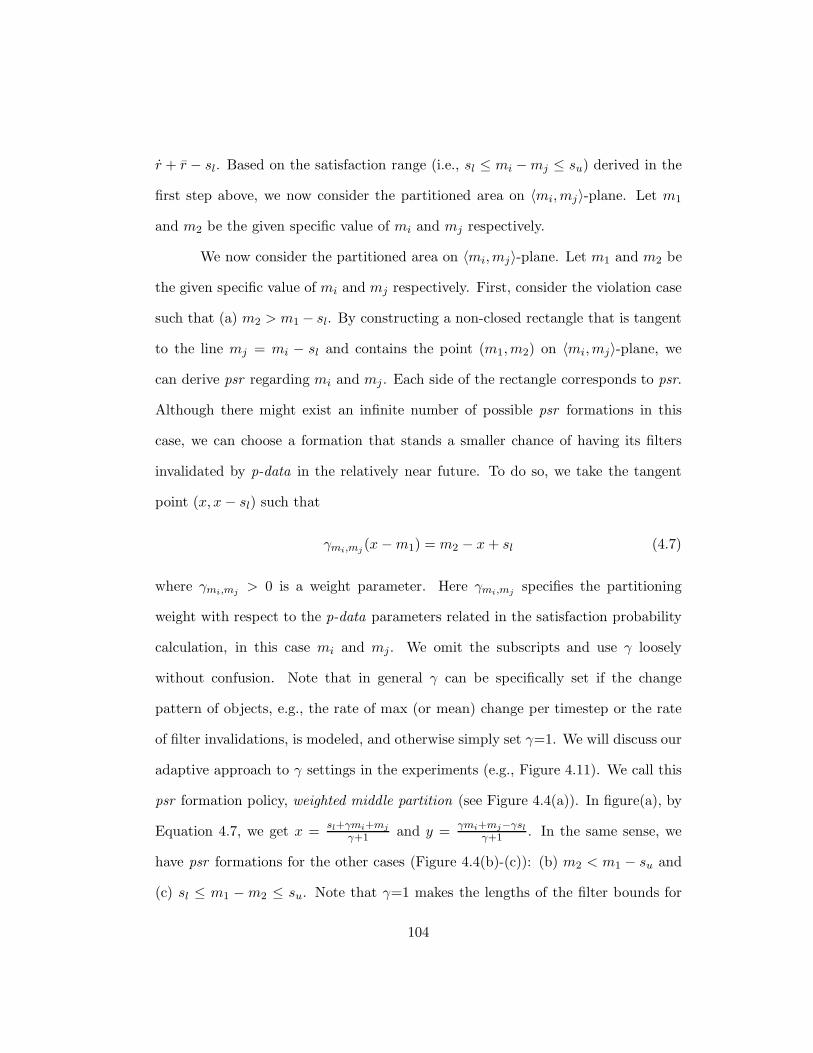
r + r − sl. Based on the satisfaction range (i.e., sl ≤ mi −mj ≤ su) derived in the
first step above, we now consider the partitioned area on 〈mi,mj〉-plane. Let m1
and m2 be the given specific value of mi and mj respectively.
We now consider the partitioned area on 〈mi,mj〉-plane. Let m1 and m2 be
the given specific value of mi and mj respectively. First, consider the violation case
such that (a) m2 > m1 − sl. By constructing a non-closed rectangle that is tangent
to the line mj = mi − sl and contains the point (m1,m2) on 〈mi,mj〉-plane, we
can derive psr regarding mi and mj . Each side of the rectangle corresponds to psr.
Although there might exist an infinite number of possible psr formations in this
case, we can choose a formation that stands a smaller chance of having its filters
invalidated by p-data in the relatively near future. To do so, we take the tangent
point (x, x− sl) such that
γmi,mj(x−m1) = m2 − x + sl (4.7)
where γmi,mj> 0 is a weight parameter. Here γmi,mj
specifies the partitioning
weight with respect to the p-data parameters related in the satisfaction probability
calculation, in this case mi and mj. We omit the subscripts and use γ loosely
without confusion. Note that in general γ can be specifically set if the change
pattern of objects, e.g., the rate of max (or mean) change per timestep or the rate
of filter invalidations, is modeled, and otherwise simply set γ=1. We will discuss our
adaptive approach to γ settings in the experiments (e.g., Figure 4.11). We call this
psr formation policy, weighted middle partition (see Figure 4.4(a)). In figure(a), by
Equation 4.7, we get x =sl+γmi+mj
γ+1 and y =γmi+mj−γsl
γ+1 . In the same sense, we
have psr formations for the other cases (Figure 4.4(b)-(c)): (b) m2 < m1 − su and
(c) sl ≤ m1 −m2 ≤ su. Note that γ=1 makes the lengths of the filter bounds for
104

éêéëìíî ïðñò óðôõö÷ïðñéø÷ïéùñò÷ïéùñéø÷
úûü úýü úþüÿ�� ������� � ������� ����������������
Figure 4.4: Weighted middle partition
mi and mj equal.
Notice that the case (c) is for satisfaction and a closed rectangle being tangent
to both lines mj = mi − sl and mj = mi − su needs to be chosen.
Finally, given specific Ui of oi and Uj of oj, we have psr(oi)|pcJ
Ui, psr(oj)|pcJ
Uj=
[-∞, g(sl)), (g(−γsl),∞] if mj > mi − sl
(g(su),∞], [-∞, g(−γsu)) if mj < mi − su
[g(sl), g(su)], [g(−γsu), g(−γsl)] otherwise
(4.8)
where g(x) =x+γmi+mj
γ+1 in case that sl and sh exist.
4.2.2 psr for Gaussian data
We denote p-data that is characterized by the gaussian distribution by Gi: (µi, σi),
noting that X ∼ N(µi, σ2i ) where X is the r.v. characterized by Gi. Such Gis will
be called gaussian data. We represent the standard normal distribution function
and its inverse function by
Φ(x) = P (z ≤ x) and Φ−1(Φ(x)) = x where z ∼ N(0, 1).
105

For simplicity in explanation, we will use, besides pcR and pcJ , the following con-
straint with a unit-length range [0, 1], the so-called unit-length constraint.
cU : 0 ≤ oi ≤ 1, pcU : (cU , δ) (4.9)
Note that psr for the unit-length constraint can be adjusted to that for any con-
straints with arbitrary ranges.
Given a set of gaussian data satisfying pcU , we obtain a non-linear curve on
the 2-dimensional mean and standard deviation parameter space, i.e., 〈µ, σ〉-plane,
by using the following inequality.
prob(cU )|Gi= Φ(
1− µi
σi)− Φ(
0− µi
σi) ≥ δ (4.10)
Although it might appear simple to locate individual points on the constraint
curve, there is no analytical solution, i.e., we do not have a closed form solution to
obtain an x that satisfies prob(cU )|(µi,x) = δ for specific values of µi and δ except
for µi=12 . Figure 4.5(a) shows an example graph of the satisfaction probability
with various gaussian data. In this figure, X-axis represents −2.5 ≤ µi ≤ 3, Y-axis
represents 0 ≤ σi ≤ 2.5, and Z-axis represents prob(cU )|(µi,σi) where cU is defined
in Equation 4.9. Figure 4.5(b) depicts its contour lines, which can be numerically
found. In this figure, X-axis represents −2.5 ≤ µi ≤ 3.5, Y-axis represents 0 ≤ σi ≤
2.5, and the curves represent prob(cU )|(µi,σi) = δ where δ = 0.1, 0.2, . . . , 0.9 (from
the most outer curve). Each contour line corresponds to the constrained curve by
Equation 4.10 and thus describes the satisfaction and violation areas for pcU with
a specific value of δ, similarly as shown in Figure 4.2(b).
Lemma 4. Given a range constraint cR: r ≤ oi ≤ r and gaussian data (µi, σi) of
106

-2
0
20.5
1
1.5
2
2.5
0
0.25
0.5
0.75
1
-2
0
2
(a) Satisfaction probability
-2 -1 0 1 2 3
0.5
1
1.5
2
2.5
(b) Constrained curves
Figure 4.5: Constrained graph for gaussian data
oi, we have
prob(cR)|(µi,σi) = prob(0 ≤ oi ≤ 1)|(µu ,σu)
where µu = µi−rr−r
and σu = σi
r−r.
Proof. prob(cR)|(µi,σi) = Φ( r−µi
σi) − Φ( r−µi
σi) = Φ(1−µu
σu) − Φ(−µu
σu) = prob(0 ≤ oi ≤
1)|(µu ,σu).
Lemma 4 allows us to transform a constrained curve of the unit-length con-
straint to that of any arbitrary range constraint with the same value of δ. Further-
107

more, we can exploit the symmetry of constrained curves. Note that all the curves
in Figure 4.5(b) are symmetric about r+r2 = 1
2 , to be consistent with the following
lemma.
Lemma 5. Given a range constraint cR: r ≤ oi ≤ r and gaussian data (µi, σi) of
oi, we have
prob(cR)|(µi,σi) = prob(cR)|(r+r−µi,σi).
Proof. prob(cR)|(r+r−µi,σi) = Φ(µi−rσi
) − Φ(µi−rσi
) = 1 − Φ( r−µi
σi) − 1 + Φ( r−µi
σi) =
prob(cR)|(µi,σi).
Interval psr for Range Constraints
Similarly as in the case of uniform data, psr for gaussian data with static variances
is given by an interval regarding µ. However, such an interval must be found numer-
ically, unlike uniform data. For efficiently updating psr -based filters at run-time, we
can pre-calculate a table, named G-table, that contains the approximate points of
the constrained curve (e.g., derived by Equation 4.10) for various values of δ of pcU .
This requires using a numerical method. In particular, to prune unnecessary sam-
pling points in our numerical calculation, we use a rectangle tightly enclosing the
constrained curve. Such rectangle is called a minimum violation rectangle (e.g., the
solid line rectangles in Figure 4.6). The implementation of our numerical method
will be described in Chapter 4.2.3. In the following, suppose we have the minimum
violation rectangle for pcU , denoted by
rcv : [µv, σv, µv, σv] (4.11)
and the following auxiliary function that provides the interface to the G-table.
108

Definition 13. For the unit-length constraint pcU :(cU , δ), we define the constrained
curve function:
G(x)|δ = µi s.t. prob(cU )|(µi,x) = δ ∧ µi ≥1
2(4.12)
for x ≥ 0. Note that given µi = G(σi)|δ, we have prob(cU )|(1−µi,σi) = δ by Lemma 5.
It is obvious that given a specific value of σi ≤ σv, (the derivation of σv is
in Equation 4.17 below), we have the partitioned satisfaction and violation ranges
regarding µi. These ranges immediately specify psr, and thus
psr(oi)|pcu
Gi=
(x,∞] if µi > x ∧ σi ≤ σv
[-∞, 1− x) if µi < 1− x ∧ σi ≤ σv
[1− x, x] if 1− x ≤ µi ≤ x ∧ σi ≤ σv
[-∞,∞] otherwise
(4.13)
where x = G(σi)|δ .
Generalization for arbitrary ranges. We have shown psr formation for the unit-
length constraint pcU above. For an arbitrary range [r, r], the psr with respect to
pcU can be adjusted by Lemma 4. For example, from (i) calculated by Equation 4.13,
we obtain (ii) below where l = r − r.
(i) psr(oi)|pcU
(µi−r
l,
σil
)= [µ, µ], (ii) psr(oi)
pcR
(µi,σi)= [lµ + r, lµ + r] (4.14)
psr for Join Constraints
Based on the linear property of the difference of independent gaussian r.v., that is,
given Gi:(µi, σi) and Gj :(µj, σj),
prob(cJ)|Gi,Gj= Φ(
r − µi + µj√
σ2i + σ2
j
)− Φ(r − µi + µj√
σ2i + σ2
j
),
109

it is possible to find the partitioned ranges regarding µi − µj by using gaussian
data Gk: (µi − µj ,√
σ2i + σ2
j ) and Equation 4.13-4.14. This allows us to find the
satisfaction range of µi − µj , denoted as sl ≤ µi − µj ≤ su. Assume a weight
parameter γ and let g(x) =x+γµi+µj
γ+1 . By the policy of weighted middle partition,
then, the respective psr of oi and oj are given same as Equation 4.8 except for here
using µi, µj instead of mi, mj.
4.2.3 Pre-calculated Table for Constrained Curves
Here we discuss how to construct the G-table and implement G(.) function in Defini-
tion 13. Note that this procedure is required only for the unit-length constraint and
can be done off-line. As mentioned before, we first derive the minimum violation
rectangle rcv (Equation 4.11) so as to efficiently restrict the range to be handled by
our numerical method. We adapt the calculation method in [18].
First, consider σv and σv in rcv. Let us denote the satisfaction probability
function of µ by
Fµ(x) = prob(cU )|(x,σi) in Equation 4.10. (4.15)
Then, using the derivative of the above function
dFµ(x)
dx=
1
σi
√2π
(− exp(−(−1 + x)2
2σ2i
) + exp(− x2
2σ2i
)) (4.16)
and the critical point x′ = 12 such that
dFµ(x′)dx
= 0, we observe that Fµ(x =
12) is the maximum (as shown by the contour lines in Figure 4.5(b)) and thus
prob(cU )|( 1
2,σv) = δ. Due to the fact that prob(cU )|( 1
2,σv) = Φ( 1
2σv) − Φ( −1
2σv) =
Φ( 12σv
) − 1 + Φ( 12σv
) holds, we have Φ( 12σv
) = δ+12 . Since Φ(.) is a monotonically
110

increasing function, we have
1
2σv= Φ−1(
δ + 1
2) =⇒ σv = (2Φ−1(
δ + 1
2))−1. (4.17)
Moreover, obviously we have
σv = 0 (4.18)
because prob(cU )|( 1
2,0) ≥ δ always holds.
Second, consider µv and µv in rcv. In the case of 0.5 ≤ δ < 1, since
prob(cU )|(1,0) = 1 holds and prob(cU )|(µi,σi) < 0.5 holds for any µi /∈ [0, 1] and
σi ≥ 0, we have
µv = 1, and accordingly µv = 0 by Lemma 5. (4.19)
Now, consider the other case: 0 < δ < 0.5. Similar to what has been done previously
for finding σv but using x = σi instead here, let us define a function
Fσ(x) = prob(cU )|(µi,x). (4.20)
By solving dFσ(x′)dx
= 0, we get x′ such that Fσ(x′) is the maximum. Such x′ is
denoted by a function of y = µi,
Fσµ (y) =
√
(2y − 1)/
ln
[
y2
(y − 1)2
]
. (4.21)
Then we may write
µv = y s.t. δ = prob(cU )|(y,Fσµ (y)), and µv = 1− µv. (4.22)
It should be noted that due to the recursive definition in the above expression,
the exact value of µv cannot be directly derived but can be numerically estimated.
Finally Equation 4.17-4.22 establish the minimum violation rectangle rcv.
111

G-table construction. SincedFµ(x)
dx= 0 (Equation 4.16) holds for x = 1
2 and
dFµ(x)dx
< 0 holds for x > 12 , it is possible to numerically find the estimate of µi
such that δ = prob(cU )|(µi,σi) by increasing the sample points sk ∈ [12 , µv] for the
given specific values of δ and σi < σv. It is important to note that due to limited
sampling steps of sk, we rather take a range estimate of µi for the satisfaction and
violation areas; for each pair (δ, σi), the range estimate [µsi , µ
vi ] is found and kept in
G-table where the exact estimate of µi should be in [µsi , µ
vi ]. Furthermore, using the
derivative of the function in Equation 4.20:
dFσ(x)
dx=
1
x2√
2π((µi − 1) exp(−(−1 + µi)
2
2x2)− µi exp(− µ2
i
2x2)),
we obtain that dFσ(x)dx
< 0 holds for 0 < µi < 1. Therefore, in the case 0.5 ≤ δ < 1
(so, µv = 1), we can restrict the necessary sample range sk along with decreasing
σi values. More specifically, given a range estimate [µsi , µ
vi ] of µi found for some
σi, the sample range for σ′i < σi is reduced to 1
2 < µsi ≤ sk ≤ µv = 1. In case of
0 < δ < 0.5, we consider two different cases: (i) σi > Fσµ (µv) (where dFσ(x)
dx< 0)
and (ii) otherwise (where dFσ(x)dx
≥ 0). Then, it is possible to reduce the necessary
sample range by increasing the lower bound (using µsi similarly as above) for the
case (i) and by decreasing the upper bound for the case (ii) along with decreasing
σi values.
Since range estimates [µsi , µ
vi ] are tabulated, the actual G(.) function needs to
return either µsi or µv
i depending on the constraint result by the given gaussian data.
For example, for the first two (violation) cases in Equation 4.13, we take G(σi)|δ =
µvi ; for the third (satisfaction) case, G(σi)|δ = µs
i . Since taking such proper bound
from a range estimate is obvious, we omit this description.
112

4.3 psr Formation with Dynamic Variances
Thus far, we have focused on psr formation with static variances. The static variance
assumption is normally suitable for modeling the tracking of object values that
are not highly dynamic i.e., they do not change drastically in a short time. In
reality, however, there are situations where the uncertainty degree of an object
fluctuates for subsequent timesteps and so it should be modeled as a variable. In
this chapter, we consider the gaussian data streams and focus on the rectangular
psr formation, incorporating the continuous updates of both µ and σ parameters to
the psr formation and filter construction.
In addition to the minimum violation rectangle rcv (Equation 4.11), we no-
tate σµ such that the point (µv, σµ) is located on rcv (see Figure 4.6(b); (µv , σµ) is
called max-µ point). And let us denote psr (e.g., psr (oi)|pcU
Gi) by a rectangle rcpsr on
〈µ, σ〉-plane. We will then show how to determine rcpsr depending on the location
of the given gaussian data. Note that in case µi < 12 , we can calculate psr with
the gaussian data (1 − µi, σi), psr(oi)|pcU
(1−µi,σi)= [µ, σ, µ, σ], using the formulae for
the case of µi ≥ 12 , and then convert it to rcpsr:[1 − µ, σ, 1 − µ, σ] according to the
symmetric property of Lemma 5. Thus, we only consider µi ≥ 12 in the following
derivation.
4.3.1 Rectangular psr Formation
Here suppose pcU |Gi= violation. First, consider the case of 0.5 ≤ δ < 1. As shown
in Figure 4.6(a), the constrained curve (i.e., G(.)) is monotonically decreasing with
respect to σi. In the figure, X-axis and Y-axis represent µi and σi; The solid line
rectangle denotes the minimum violation rectangle. Thus, in this case, we prefer
113

�� !"#$%"&'( )*+),( 11 σµ
,- )1( −iµγ./01232141 526789263:;<983=7;>?@ABC?@D BEFB
),( yxGBC?GH BIC?@D BEFBvi σµγ +− )5.0(
vσ
vµ
�J !"#$%"&'( )*Kµσ
vi σµγ +− )5.0(
µσµµγ +− )( iv
vµ
µσµµγ +− )( vi
./01232141 526789263:;<983=7;
GBC?GH BIC?@D BEFB>?@ABC?@D BEFB
vσ
Figure 4.6: psr for pcU
rcpsr the lower-left corner (x, y) of which is tangent to the constrained curve, so rcpsr
is in the form [x, y,∞,∞]. As describe before, such (x, y) is determined based on
the weighted middle partition; if (x, y) cannot exist by the relation of rcv and the
given gaussian data, we take either the upper-side or the right-side of rcv instead.
114

Then, given specific Gi such that pcU |Gi= violation, we have (x, y) =
(-∞, σv) if γ(µi − 12 ) + σv ≤ σi
(µv, 0) if γ(µi − µv) ≥ σi
(G(y)|δ , y = γ(G(y)|δ − µi) + σi) otherwise
(4.23)
where γ is a weight parameter for modeling the change pattern of oi (e.g., the change
ratio between gaussian parameters). Note that y otherwise in the case above is not
directly calculated but a binary search on G-table can rapidly locate it thanks to
the aforementioned monotonicity property. And µv = 1 necessarily holds (Equa-
tion 4.19). The gray rectangle in Figure 4.6(a) depicts the third case psr in above
Equation 4.23 for the given specific gaussian data (µ1, σ1).
Second, consider the other case 0 < δ < 0.5. Different from the previous
case, G(.) is convex around the max-µ point (µv, σµ) as shown in Figure 4.6(b).
We have the similar result to the previous case if σi ≥ γ(µv − µi) + σµ holds.
Otherwise, we find the rectangle rcpsr whose the upper-left corner (x, y) is tangent
to the constrained curve, which is
[x = G(y)|δ , 0,∞, y = γ(µi − G(y)|δ) + σi]. (4.24)
Now suppose pcU |Gi= satisfaction. In this case, psr is in the closed rectangle
inside the constrained curve. If 0.5 ≤ δ < 1 holds, obviously rcpsr is given by
[1− G(y)|δ , 0,G(y)|δ , y = γ(G(y)|δ − µi) + σi].
For x ≥ 1 and 0 < δ < 0.5, let
g1(x) = σ s.t. G(σ)|δ = x ∧ σ > σµ, g2(x) = σ s.t. G(σ)|δ = x ∧ σ ≤ σµ.
115

If 0 < δ < 0.5 holds, rcpsr can be given by
[1− x1, 0, x1, y1] if γ(µi − 1) + g1(1) ≤ σi
[1− x1, g2(x1), x1, y1] if σµ ≤ σi < γ(µi − 1) + g1(1)
[1− x2, y2, x2, g1(x2)] if γ(1 − µi) ≤ σi < σµ
[0, 0, 1, g1(1)] otherwise
(4.25)
where x1 = G(y1)|δ, y1 = γ(G(y1)|δ−µi)+σi, x2 = G(y2)|δ, and y2 = γ(µi−G(y2)|δ)+
σi.
Generalization for arbitrary ranges. Equation 4.14 is extended for rectangular
psr, psr(oi)pcR
(µi,σi)as in (ii) below.
(i) psr (oi)|pcU
(µi−r
l,σil
)= [µ, σ, µ, σ], (ii) [lµ + r, lσ, lµ + r, lσ] (4.26)
Example 11. Suppose we have pc:(−10 ≤ oi ≤ 10, 0.2) and G1:(30, 10), G2:(5, 25)
of oi, and assume the weight parameter γ=12 . As shown in Figure 4.7 and Equa-
tion 4.26, we first calculate psr(oi)|(cU ,0.2)G′
1:(2,0.5)
and psr(oi)|(cU ,0.2)G′
2:(0.75,1.25)
for G1 and
G2 respectively (as in (i), G′1=(30+10
20 , 1020 ) and G′
2=(5+1020 , 25
20 ), and then convert
them to psr (oi)|pcG1
=[21.3, 0,∞, 14.2] and psr (oi)|pcG2
=[−20.1, 12.42, 20.10, 32.69]. In
the figure, X-axis and Y-axis represent µi and σi. The gray rectangles denote
psr (oi)|(cU ,0.2)(2,0.5) =[1.56, 0,∞, 0.74] and psr(oi)|(cU ,0.2)
(0.75,1.25)=[−0.5, 0.62, 1.5, 1.63].
4.3.2 psr for Join Constraints
By the property of gaussian data explained in Chapter 4.2.2, given Gi of oi and
Gj of oj , it is possible to calculate the intermediate psr form regarding µi − µj
116

LM N M OPQRSSQRT
UVWXY Z
Figure 4.7: psr with respect to (cU , 0.2)
and√
σ2i + σ2
j , from which the respective psr of oi and oj can be derived. Suppose
we obtain such intermediate psr as a rectangle [µp, σp, µp, σp] by the formulae in
Chapter 4.3.1. Since we have presented our method to derive the respective psr
part for µi and µj in Chapter 4.2.2, here we explain its complementary part. From
the condition σp ≤√
σ2i + σ2
j ≤ σp given by the aforementioned intermediate psr,
we derive the individual range predicates on each σi and σj. Note that combining
the range predicate on σi and that on µi completes the psr of oi. In the following,
assume a weight parameter γ for modeling the difference of the change patterns of
σi and σj , supposing given specific σ1 of oi and σ2 of oj . For notational simplicity,
let
g(x) =γ2σ1 − γσ2 +
√
x2 − (σ2 + (x− σ1)γ)(σ2 − (σ1 + x)γ)
1 + γ2.
First, if σp > 0 and σp =∞, we have
σi ≥ x and σj ≥√
σp2 − x2
117

where
x =
0 if γσ1 + σp ≤ σ2
g(σp) if γ(σ1 − σp) < σ2 < γσ1 + σp
σp otherwise.
Note that Figure 4.8(a)-(b) show the different psr formations according to the first
two cases in the above equation. Each gray rectangle with solid lines denotes the
range predicates (or psr part) on σi and σj depending on the given specific σ pair
(σ1, σ2). Also note that as shown in figure(b), x = g(σp) is the tangent point on the
σi-axis, which is found by solving
γ(x− σ1) + σ2 =√
σ2p − x2.
Second, if σp = 0 and σp 6=∞, as in Figure 4.8(c) we have
σi ≤ g(σp) and σj ≤√
σ2p − (g(σp))2.
Third, if σp > 0 and σp 6= ∞, from the above two cases, we find a rectangle being
enclosed by two quadrants as in the examples in Figure 4.8(d).
We have
x ≤ σi ≤ y,√
σp2 − x2 ≤ σj ≤
√
σp2 − y2
where x and y are respectively given by
0, g(σp) if γσ1 + σp ≤ σ2
g2(σp), g(σp) if γ(σ1 − σp) < σ2 < γσ1 + σp
σp, g(σp) otherwise.
Otherwise, the range of σi and σj is the same as each domain.
118
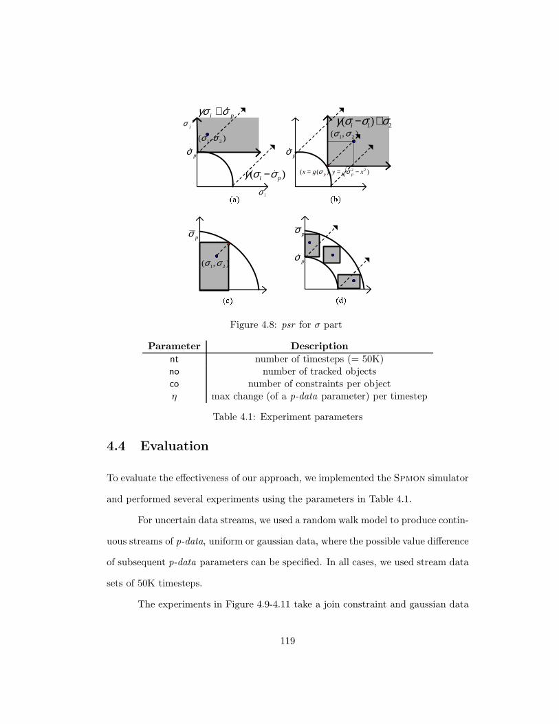
[\]),( 21 σσ
pi σγσ ^+
iσ
jσ
)( pi σσγ _−
),( 21 σσ
pσ
)),(( 22 xygx pp −== σσ aa 21)( σσσγ +−i
bcdpσ
bed bfd),( 21 σσ
pσ pσ
pσgFigure 4.8: psr for σ part
Parameter Description
nt number of timesteps (= 50K)no number of tracked objectsco number of constraints per objectη max change (of a p-data parameter) per timestep
Table 4.1: Experiment parameters
4.4 Evaluation
To evaluate the effectiveness of our approach, we implemented the Spmon simulator
and performed several experiments using the parameters in Table 4.1.
For uncertain data streams, we used a random walk model to produce contin-
uous streams of p-data, uniform or gaussian data, where the possible value difference
of subsequent p-data parameters can be specified. In all cases, we used stream data
sets of 50K timesteps.
The experiments in Figure 4.9-4.11 take a join constraint and gaussian data
119
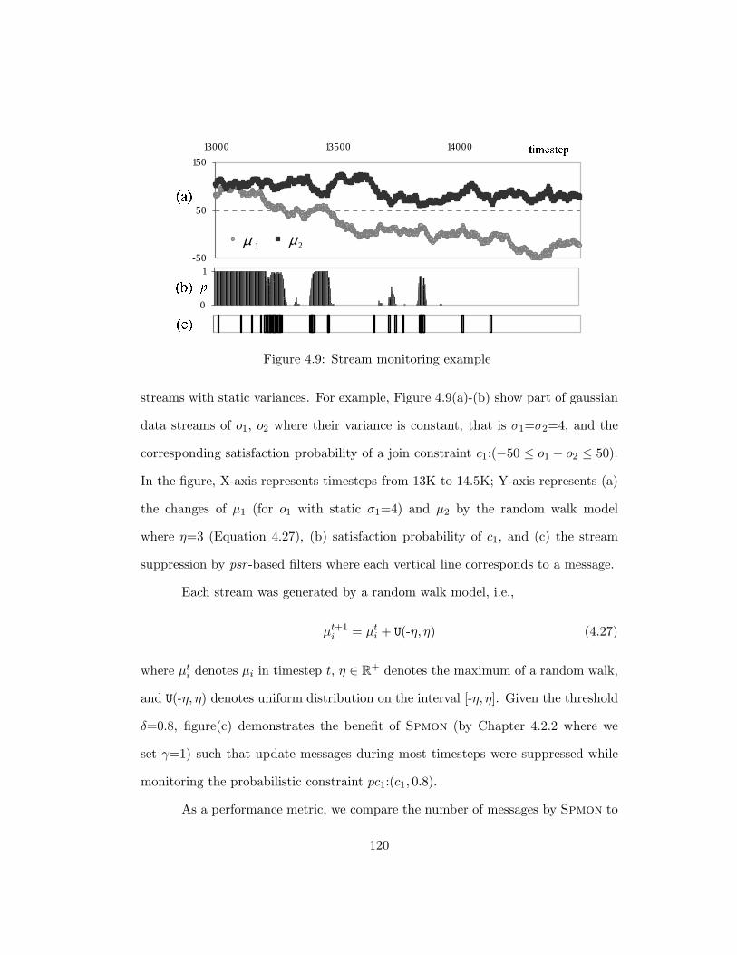
hijkilkimk
0
1
nopqrnqs-50
50
150
13000 13500 14000
m_1 m_21µ 2µ
Figure 4.9: Stream monitoring example
streams with static variances. For example, Figure 4.9(a)-(b) show part of gaussian
data streams of o1, o2 where their variance is constant, that is σ1=σ2=4, and the
corresponding satisfaction probability of a join constraint c1:(−50 ≤ o1 − o2 ≤ 50).
In the figure, X-axis represents timesteps from 13K to 14.5K; Y-axis represents (a)
the changes of µ1 (for o1 with static σ1=4) and µ2 by the random walk model
where η=3 (Equation 4.27), (b) satisfaction probability of c1, and (c) the stream
suppression by psr -based filters where each vertical line corresponds to a message.
Each stream was generated by a random walk model, i.e.,
µt+1i = µt
i + U(-η, η) (4.27)
where µti denotes µi in timestep t, η ∈ R
+ denotes the maximum of a random walk,
and U(-η, η) denotes uniform distribution on the interval [-η, η]. Given the threshold
δ=0.8, figure(c) demonstrates the benefit of Spmon (by Chapter 4.2.2 where we
set γ=1) such that update messages during most timesteps were suppressed while
monitoring the probabilistic constraint pc1:(c1, 0.8).
As a performance metric, we compare the number of messages by Spmon to
120

that by a traditional centralized monitor where p-data are transmitted to a stream
processor in every timestep. We compute the message transmission rate (msg) by
msg =nm
nt× no
where nm is the number of messages. For messages in Spmon,
nm = nivd + 2nprb + nudt (4.28)
where nivd denotes the number of psr -based filters that are invalidated by p-data;
nprb denotes the number of probes initiated by a stream processor to retrieve the
p-data of the other object in the join when the filter of one object is invalidated; and
nudt denotes the number of psr -based filter updates. Recall that the re-evaluation of
a join constraint upon invalidation by the p-data of an object oi passing through its
filter may require probing to the other object in the join in which oi appears. Owing
to these probes (more specifically, probing request and reply messages) and filter
update messages, in general, query-aware filtering methods are not always of benefit
to message reduction. We will show the effect of the overhead in Figure 4.12, in some
cases with relatively large η and co. It is also important to note that one cannot
simply use a variant of centralize monitor that uses “constant” filter ranges for our
problem, since even a minimum value change of a p-data parameter in the domain
of real numbers may require the revalidation of its associated constraints; in fact,
this is also a reason why monitoring specific continuous queries (e.g., probabilistic
constraints in this chapter, spatial queries [52]) is different from tracking time-
varying data [40, 41] which is independent of query types, although both often aim
at the same goal of low communication overhead.
Single join constraint. Figure 4.10 shows msg of monitoring a single join con-
121
tuv wxyz{|u}y{ |~z��{ ���u{~z 0
0.25
0.5
20 160 300
ms g
0
0.25
0.5
0.1 0.3 0.5 0.7 0.9
ms g
0
0.25
0.5
0.1 4.6 9.1
ms g
t�v �u� ��uy�~t�v ��|~z�x��t�v �x}y �xyz{|u}y{ |uy�~0
500
1000
20 160 300
# Cupda te
Figure 4.10: msg with various settings
straint. Figure(a) shows the number of constraint result updates depending on the
join constraint range size. In figures(b)-(d), Y-axis represents msgand X-axis rep-
resents (b) join constraint range size rs, (c) threshold δ, and (d) max change per
timestep η. Figures(b)-(d) show msg of monitoring (−rs2 ≤ o1 − o2 ≤ rs
2 , δ) where
(b) δ=0.8, η=3, (c) rs=100, η=3, (d) rs=100, δ=0.8. We set γ=1 for all the cases.
As expected and shown in figures(a)-(b), msg is heavily dependent on the degree of
fluctuation in the results of constraint evaluation over time; more dynamicity in the
tracked objects (i.e., larger η) is likely to change the constraint results rapidly and
accordingly break psr -based filters more, thus resulting in larger msg as shown in
the figure(d).
As explained, psr consists of simple predicates on p-data parameters and our
psr formation formulae contain weight parameters γ. Figure 4.11 demonstrates the
impact of this γ setting against streams with different properties. In the figure, Y-
122
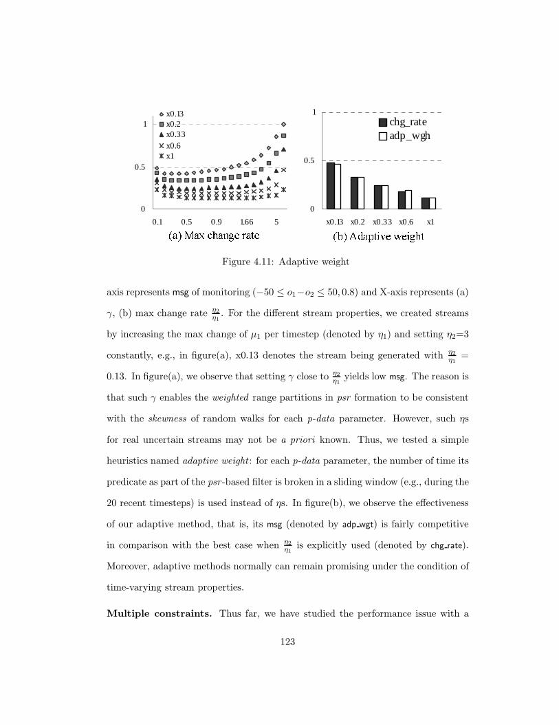
��� ��� ������ ����0
0.5
1
0.1 0.5 0.9 1.66 5
x0.13x0.2x0.33x0.6x1
0
0.5
1
x0.13 x0.2 x0.33 x0.6 x1
chg_rateadp_wgh
����������� ������Figure 4.11: Adaptive weight
axis represents msg of monitoring (−50 ≤ o1−o2 ≤ 50, 0.8) and X-axis represents (a)
γ, (b) max change rate η2
η1. For the different stream properties, we created streams
by increasing the max change of µ1 per timestep (denoted by η1) and setting η2=3
constantly, e.g., in figure(a), x0.13 denotes the stream being generated with η2
η1=
0.13. In figure(a), we observe that setting γ close to η2
η1yields low msg. The reason is
that such γ enables the weighted range partitions in psr formation to be consistent
with the skewness of random walks for each p-data parameter. However, such ηs
for real uncertain streams may not be a priori known. Thus, we tested a simple
heuristics named adaptive weight : for each p-data parameter, the number of time its
predicate as part of the psr -based filter is broken in a sliding window (e.g., during the
20 recent timesteps) is used instead of ηs. In figure(b), we observe the effectiveness
of our adaptive method, that is, its msg (denoted by adp wgt) is fairly competitive
in comparison with the best case when η2
η1is explicitly used (denoted by chg rate).
Moreover, adaptive methods normally can remain promising under the condition of
time-varying stream properties.
Multiple constraints. Thus far, we have studied the performance issue with a
123

single constraint using psr. Two major observations were that (1) msg is mainly
influenced by the dynamicity of p-data and (2) our adaptive weight policy works
quite well, not needing a priori knowledge of stream properties. Here we discuss the
case of multiple constraints with dynamic variances (for gaussian data streams in
Chapter 4.3). We created different sets of objects and constraints randomly using
given values for the parameters no, co, the range size of each constraint rs ∈ [50, 120],
and the threshold δ ∈ (0, 1). Given co=k, we created ⌈k2⌉ range constraints and ⌊k2⌋
join constraints for each object. We also created different sets of data streams using
given η of µ and σ for each object. Figure 4.12 shows that msg is also influenced by
co while it is not directly influenced by the size of object or constraint set as long
as co is same. This is because psr of an object is achieved by the intersection of psr
with respect to all the constraints being imposed on the object. In other word, a
filter region is likely to shrink more along with larger co, implying that the benefit
of Spmon could increase with small co and thus Spmon must be used conservatively
otherwise; e.g., it seems advantageous to use Spmon for the cases where co≤ 4 and
η < 3. In the figure, Y-axis represents msg and msg n denotes the different streams
of which η of µ and σ are given n and n2 respectively. X-axis represents (a) no and
(b) co. We set (a) co=2 and (b) no=10.
Finally we note that adaptiveness of Spmon such as combining the psr -based
filter and non-filtering of centralized monitor for different stream and constraint
properties is an interesting issue but is not included here due to the space limit.
124

0
0.5
1
1 2 3 4
msg_1msg_2msg_3msg_4
�� ¡¢£¤¥¦§¨£¥¤ ©ª¦ ¢�«ª¬¥ �¬¢ 0
0.5
1
10 20 30 40 50
msg_3
�§ �«ª¬¥ ¤ª¥ �£¢ Figure 4.12: Multiple constraints
4.5 Summary
As usage of sensor-based real-time monitoring systems grows, probabilistic data
processing based on statistical modeling techniques has gained much attention in
both the stream database and real-time database literature [10, 15, 30]. In this
chapter, we have presented Spmon, a monitoring architecture that incorporates
data value uncertainty in monitoring constraint-based queries. In particular, we
have generalized the notion of data similarity to cover data objects whose values
can only be determined probabilistically. To the best of our knowledge, Spmon
is the first to attempt monitoring and filtering of uncertain data streams in pdf
parameter spaces. As shown, the filter conditions based on the new psr concept can
be systematically derived for well-known distributions.
Although we believe Spmon is general enough to incorporate different data
models, it should be noted that the derivation for psr formation can be challenging
depending on distributions. However, our work for uniform and gaussian models
could be a reference for further development, particularly for other distributions
with one or two pdf parameters, that is, those specifying location and variance
properties in the pdf definition.
125

Chapter 5
Conclusion and Future Work
5.1 Ongoing and Future Work
There are several directions to extend the work in this dissertation. Some of them
are described here.
5.1.1 Efficient Monitoring based on Analysis for System Safety Ver-
ification
Model-based development has been recognized as a practical method for efficiently
developing correct and robust control-oriented real-time embedded systems. In
general model-based development has focused on verification and testing for func-
tional or timing aspects. However, embedded software also involves para-functional
resource-related aspects. Such para-functional resource-related aspects of embedded
software are termed resource (bound) properties. These properties enforce resource
limits on CPU time, memory, battery power, network bandwidth, etc. Unlike func-
tional properties, yet the verification and testing for resource properties has not
126

been completely addressed in executable model-based development. Specifically
resource-related language constructs are not incorporated in the action semantics
of executable models since early design is intended to be platform independent.
Accordingly resource properties have not been entirely linked with functional veri-
fication from the beginning of the development cycle. This limitation often renders
the process of resource safety verification (the verification of resource bound prop-
erties) non-systemic or ad hoc at best leading to excessive cost for monitoring and
analysis. Furthermore, resource safety verification is usually deferred to testing
during/after the implementation phase. Resource safety violations detected dur-
ing implementation testing commonly require redesign and reimplementation of the
system.
Recently we proposed the software engineering discipline incorporating re-
source safety verification into a design and development methodology for embedded
systems in [64, 62, 59]. This work focuses on how to integrate the verification of
para-functional resource properties into the software development cycle of executable
model-based approaches. The proposed methodology integrates:
• xUML (eXecutable Unified Modeling Language [42]) modeling and simulation-
based model testing processes supported by the commercial software modeling
and simulation environment Objectbench [54]
• Automatic code generation from xUML models by CodeGenesis code genera-
tor [53]
• Formal functional verification by model checking for xUML models [63]
• Resource bound checking based on static analysis and dynamic monitoring [48,
127
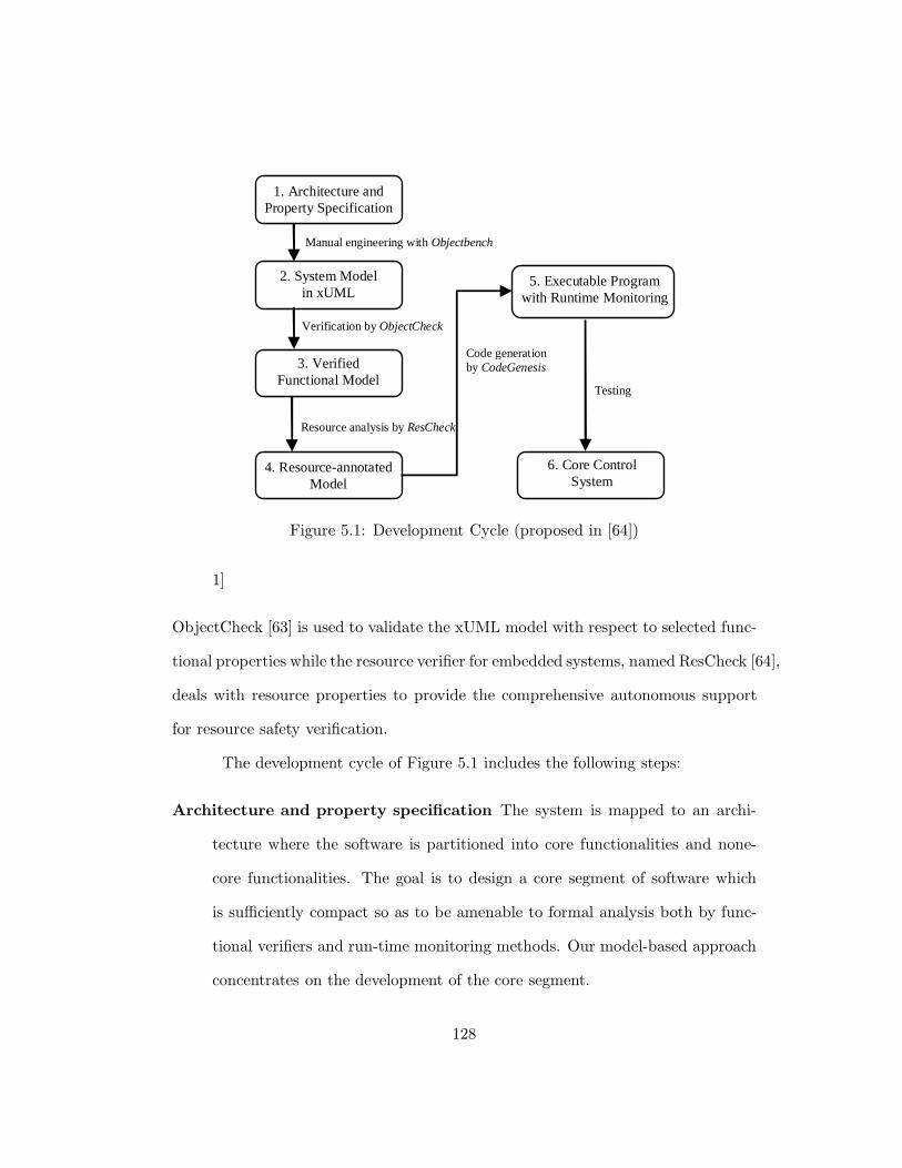
1. Architecture and
Property Specification
2. System Model in xUML
3. Verified Functional Model
4. Resource-annotated Model
5. Executable Program with Runtime Monitoring
6. Core Control System
Manual engineering with Objectbench
Verification by ObjectCheck
Resource analysis by ResCheck
Code generation by CodeGenesis
Testing
Figure 5.1: Development Cycle (proposed in [64])
1]
ObjectCheck [63] is used to validate the xUML model with respect to selected func-
tional properties while the resource verifier for embedded systems, named ResCheck [64],
deals with resource properties to provide the comprehensive autonomous support
for resource safety verification.
The development cycle of Figure 5.1 includes the following steps:
Architecture and property specification The system is mapped to an archi-
tecture where the software is partitioned into core functionalities and none-
core functionalities. The goal is to design a core segment of software which
is sufficiently compact so as to be amenable to formal analysis both by func-
tional verifiers and run-time monitoring methods. Our model-based approach
concentrates on the development of the core segment.
128
xUML model The executable model in xUML for the core segment is manually
developed by using Objectbench. Objectbench is a software development tool
that supports a UML-like OOA method [42] and generates executable and com-
pilable specifications for analysis models. The model is executed and tested
under the control of the discrete event simulator in Objectbench.
Verified functional model The model is formally verified with respect to the
selected functional properties by the xUML model checking tool ObjectCheck.
The xUML specification of the model is automatically translated to the S/R
model specification to be verified by COSPAN model checker [25]. The details
of xUML model checking can be found in [63].
Resource-annotated model The model is further specified by manually adding
resource-related specification into the functional specifications. At present our
approach (implemented and tested in [64]) requires the developers to write the
partial implementation code of resource-related operations and insert it to the
executable state actions of the state model in xUML. Note that the language
constructs for resource specification in xUML models can be developed to
provide the appropriate abstraction of resource specification. The model is
then analyzed by ResCheck. As a result, violations of resource properties can
be detected at this design phase and the model revised accordingly. Run-time
monitoring code for resource safety verification is automatically inserted in the
action specifications in the model for those resource properties that cannot
be statically verified. By using a low overhead run-time monitoring scheme,
ResCheck supports efficient dynamic evaluation of resource consumption upper
bounds. The detailed procedure for static resource analysis and monitoring in
129

ResCheck can be found in [64].
Executable program The model is automatically translated into executable pro-
gram code via CodeGenesis code generator [4] for a particular target platform.
Based on the resource-annotated model specification derived from the static
resource analysis in the previous step, the generated program contains the
minimum necessary monitoring code. Then the program is run and tested
on the target platform. Run-time violations of resource properties can be de-
tected and reported. Resource safety violation rates above critical thresholds
may require redesign.
Core control system The model satisfying all the functional and resource prop-
erties is ready to be extended with the further design and implementation for
non-core functionalities. It is important to note that the development cycle in
Figure 5.1 can be iterated until the software implementation for core segment
is verified by model checking (the task spanning box 2 to 3 in Figure 5.1) and
testing with run-time monitoring (the task spanning from the box 4, 5 to 6)
In the development methodology above, verification for functional or resource
properties is done by combining model checking, resource analysis and run-time
monitoring. As mentioned, using xUML model checking for functional properties
has been well studied by in [63], which is briefly introduced in the following. In
ObjectCheck, designers of the system use the Property Specification Interface and
xUML Visual Modeler to specify the properties of the system and xUML model. An
xUML-to-S/R translator converts them to S/R query and S/R model respectively.
The COSPAN model checker accepts these inputs and checks whether the query
130

is valid in the model. In case that the verification fails, COSPAN model checker
generates an error track and then Error Report Generator produces an error report
in xUML from the error track. To help the debugging process, Error Visualizer
creates a test case from the error report and reproduces the error by running the
xUML model with the test case.
The complementary problem, efficient run-time monitoring has been intro-
duced in [64] where resource properties are treated as the primary concern on verifi-
cation. Notice that due to their inherently dynamic nature, resource properties are
not usually addressed in the static-verification-only context. It is also important to
note that resource properties can be translated in the form of continuous constraint
queries in Chapter 4.
The work in [64] primarily aims at incorporating the verification process
for resource-related properties into the early development cycle, thereby lowering
development cost and enhancing the quality of resource critical embedded software.
Resource safety verification requires additional resource-related specification in the
model as input to further analysis at the design phase. It is worthwhile to note,
however, the developer’s labor can be reduced by exploiting the executable semantics
of xUML and the autonomous tool support for resource analysis and monitoring code
insertion. The executable semantics of xUML enables the model specification to be
tested in the simulation environment and to be automatically translated into an
executable program [42, 63], and furthermore it allows resource-related operations
to be specified as part of state actions in the state model.
The approach in [64] employs a hybrid framework where static analysis and
monitoring techniques cooperatively work to provide resource safety verification. In
131

the framework, the run-time monitoring makes explicit use of static analysis results
to cope with the possible performance overhead of traditional run-time monitor-
ing mechanism. To do so, the static analysis in the framework first translates a
given executable model containing resource-related code into a tree-based resource
evaluation structure.
The resource evaluation structure may involve statically-unbounded variables
e.g., loop bounds that can only be dynamically determined. This often renders
the verification inherently incomplete at analysis time and necessitates run-time
monitoring support. For monitoring efficiency, the static resource analysis simplifies
run-time operations by having in-lined monitoring code.
The run-time monitoring relies on static analysis and thus monitors discrete
updates of a small set of specific variables in the program execution, instead of di-
rectly tracking and managing dynamic resource usage information. Since in practice
testing alone cannot completely guarantee system correctness, it is natural that a
product system employs run-time monitoring support at the execution environment
as part of exception handling. This would in turn incur inordinate performance
overhead to the execution environment unless the monitoring algorithm is carefully
designed. The hybrid framework specifically, lightweight monitoring based on static
analysis results, addresses this problem of run-time overhead. More importantly, it
can cover a wide variety of property types in software safety requirements.
This hybrid framework is consistent in the recent work [1]. Ajay et al. [1] first
classifies the extant work on program resource verification into static, dynamic, and
hybrid approaches. The dynamic approaches have an advantage in that they can
be implemented easily; however, they introduce extra run-time overhead for moni-
132
toring. On the other hand, static approaches do not impose the run-time overhead.
But they depend on program analysis requiring complex implementations and some-
times they cannot be done completely [1]. Furthermore if resource bounds depend
on dynamic data which are known only during run-time, then pure static analysis
may fail to check the resource bounds. Dynamic approaches include [32, 4, 12].
Most of the research taking the dynamic approach supports Java and converts the
byte code of the source program to a functionally equivalent code appended with
run-time monitoring for resources. Since most languages lack fine-grained resource
control mechanism, many dynamic approaches provide resource management inter-
face so that users can design various policies. Crary and Weirich’s work [6] is a
purely static approach. It uses virtual clocks to augment a program and certifies
that the program does not exceed its resource boundary by showing that the virtual
clocks cannot expire.
The critical functionalities identified in a system design can be verified by
model checking and/or completely tested in the development cycle above, and then
the corresponding software component can be treated as core segment. The hybrid,
lightweight monitoring technique is also naturally consistent with desirable exten-
sion to the implementation and integration of non-core segment where the static
verification may be inherently limited. The monitoring technique for providing the
safe interplay between core and non-core segments of a control-oriented embedded
system is one of our future directions. Out-stream of unreliable components and
dynamic environmental information can be relatively unreliable to some extent, thus
necessitating probabilistic approach for handling those information streams.
133

5.1.2 Monitoring and Filtering Framework
As for dealing with the uncertainty of data values and monitoring data constraints,
we have considered a specific case when uncertain data values in streams are char-
acterized by gaussian or uniform distribution. For extensibility, it is desirable to
have a set of model-independent function specifications for the monitoring and fil-
tering of uncertain data streams as an underlying layer in the monitoring system,
similarly to what we have done in Ptmon for monitoring timing constraints. Given
specifications, it is possible to show how to efficiently realize them within different
data models, e.g., with arbitrary histogram distributions.
In practice, we can often predict the near-term data values of dynamic ob-
jects, by understanding their update pattern [21, 28]. For example, the future loca-
tion of a moving object can be predicted by combining the current position and the
speed of the object in the future speculation, and some environmental attribute in
process controls may show a certain type of correlation with other related attributes.
Owing to distributed data sources in typical sensor-based applications, data streams
are likely to contain delayed information, but in general, data streams need to be
processed in real-time. Thus it is worthwhile to provide a systematic method for
integrating some promising predictive data models to the real-time monitoring ar-
chitecture, thus enabling end-users to control the quality and the responsiveness
of a monitoring task. Our monitoring framework can be extended to incorporate
predictive data stream models for this purpose.
134

5.1.3 Extended Stream Timing Joins
A composite event resulting from the timing correlation of imprecise instantaneous
events incurs uncertainty on an activity that spans a time period. If event times-
tamp values are given as time points, in general, such a period is denoted as two
time points, the starting time and the terminating time of the activity. To handle
uncertainty, however, it is natural to consider the uncertain timestamp model where
two pdf s are associated with their respective time intervals for starting and termi-
nating times. In correlating period events, an intersection operator is fundamental.
For example, suppose we have a monitoring query based on the intersection for a
surveillance system, that is “if the probability that acoustic signals and seismic sig-
nals from near locations instantly intersect at least 0.2 sec exceeds the confidence
threshold 0.9, then raise alarm for possible intrusion.” The monitoring condition
can be written as
P (min(Xa, Xs)− 0.2 ≥ max(Xa, Xs)) ≥ 0.9
where Xa and Xs (Xa and Xs) are r.v. on the terminating (starting) times of the
acoustic signal event and the seismic signal event. A unified stream join method for
handling both uncertain instant events and periodic events would be rather desirable
as an extension of Ptjoin.
5.2 Conclusion
In recent years, it has been often argued by the real-time community that program-
ming models for embedded real-time applications are more naturally expressible
in terms of data and event streams as first class objects and operators on these
135

objects [38]. In this dissertation, we have undertaken the research to study the
monitoring of real-time event and data streams under uncertainty in either event
timing or data values. Uncertainty has been regarded as a very common problem
upon the rapid emergence of various sensor-based real-time monitoring applications
for which the disparity between values in these application databases and the actual
target attributes in the physical world cannot be easily avoided [8].
Our broad framework is to think of these applications as a special type of data
management systems where a query engine is used to answer questions about the cor-
relation of events. In general, events have attributes including timestamp, location,
data fields. The query form in the monitoring framework is based on a propositional
version of the real time logic so as to represent the relation of events as monitoring
queries. Our work focuses on the definition of operators on the event attributes and
their efficient implementation by exploiting the attribute-specific properties such as
the monotonicity of timestamps while allowing the uncertainty in temporal and data
values.
In this dissertation, we have first addressed the problem of event-based mon-
itoring with uncertainty. The proposed timing monitoring framework Ptmon incor-
porates the uncertainty of the difference between event occurrences and detections
in the monitoring of timing constraints over events. The framework provides a
generalized and modular scheme for expediting the detection of timing constraint
violations, and can be specifically realized along with different uncertainty models.
We have also showed how this framework can be used for a timing join operator
Ptjoin in the context of stream data management. Ptjoin can be seen as the
implementation of a time-window-based stream join but with the assumption of
136

probabilistic timestamp models.
We have then presented a new monitoring approach to cope with uncertainty
for data values on underlying data streams. By exploring the notion of similarity
in the real-time database literature, we have focused on the stream monitoring and
filtering technique Spmon that suppresses the degree of update redundancy on data
streams. Notice that the value uncertainty in Spmon is orthogonal to the timing
uncertainty in Ptmon for processing events and continuous queries in stream data
management. And accordingly the integrated approach for both uncertainties would
be required in case complex event queries exist.
137

Bibliography
[1] C. Ajay, E. David, and I. Nayeem. Enforcing Resource Bounds via Static Verifica-
tion of Dynamic Checks. ACM Transactions on Programming Languages and Systems
(TOPLAS), 29(5), January 2007.
[2] M. Amirijoo, N. Chaufette, J. Hansson, S. H. Son, and S. Gunnarsson. Generalized
Performance Management of Multi-Class Real-Time Imprecise Data Services. In Proc.
of IEEE Real-Time Systems Symposium(RTSS), pages 38–49, December 2005.
[3] T. Anderson, M. Moran, S. Ketcham, and J. Lacombe. Tracked Vehicle Simulations and
Seismic Wavefield Synthesis in Seismic Sensor Systems. IEEE Computing in Science
and Engineering, 6(6):22–28, November/December 2004.
[4] W. Binder and J. Hulaas. A Portable CPU-Management Framework for Java. IEEE
Internet Computing, 8(5), 2004.
[5] D. Carney, U. Cetintemel, M. Cherniack, C. Convey, S. Lee, G. Seidman, M. Stone-
braker, N. Tatbul, and S. Zdonik. Monitoring Streams: A New Class of Data Man-
agement Applications. In Proc. of the International Conference on Very Large Data
Bases(VLDB), pages 215–226, 2002.
[6] S. Chakravarthy, V. Krishnaprasad, E. Anwar, and S. K. Kim. Composite Events for
Active Databases: Semantics, Contexts and Detection. In Proc. of the International
Conference on Very Large Data Bases(VLDB), pages 606–617, August 1994.
[7] D. Chen and A. K. Mok. SRDE: Application of Data Similarity to Process Control. In
Proc. of IEEE Real-Time Systems Symposium(RTSS), pages 136–145, December 1999.
138

[8] R. Cheng, D. V. Kalashnikov, and S. Prabhakar. Evaluating Probabilistic Queries
over Imprecise Data. In Proc. of the ACM SIGMOD International Conference on
Management of Data, pages 551–562, 2003.
[9] R. Cheng, B. Kao, S. Prabhakar, A. Kwan, and Y. Tu. Adaptive Stream Filters for
Entity-based Queries with Non-value Tolerance. In Proc. of the International Confer-
ence on Very Large Data Bases(VLDB), pages 37–48, August 2005.
[10] R. Cheng, Y. Xia, , S. Prabhakar, R. Shah, and J. S.Vitter. Efficient Indexing Methods
for Probabilistic Threshold Queries over Uncertain Data. In Proc. of the International
Conference on Very Large Data Bases(VLDB), pages 876–887, August 2004.
[11] S. E. Chodrow, F. Jahanian, and M. Donner. Run-time Monitoring of Real-time Sys-
tems. In Proc. of IEEE Real-Time Systems Symposium(RTSS), pages 74–83, December
1991.
[12] G. Czajkowski and T. Eicken. JRes: A Resource Accounting Interface for Java. In
OOPSLA, pages 21–35, Octobor 1998.
[13] A. Deshpande, C. Guestrin, and S. Madden. Using Probabilistic Models for Data
Management in Acquisitional Environments. In Proc. of Conference on Innovative
Data Systems Research(CIDR), pages 317–328, 2005.
[14] A. Deshpande, C. Guestrin, S. Madden, J. Hellerstein, and W. Hong. Model Driven
Data Acquisition in Sensor Networks. In Proc. of the International Conference on Very
Large Data Bases(VLDB), pages 588–599, 2004.
[15] A. Deshpande and S. Madden. MauveDB: Supporting Model-based User Views in
Database Systems. In Proc. of the ACM SIGMOD International Conference on Man-
agement of Data, pages 73–84, June 2006.
[16] C. E. Dyreson and R. T. Snodgrass. Supporting Valid-time Indeterminacy. ACM
Transactions on Database Systems, 23(1):1–57, March 1998.
[17] J. Enderle, M. Hampel, and T. Seidl. Joining Interval Data in Relational Databases. In
Proc. of the ACM SIGMOD International Conference on Management of Data, pages
683–694, 2004.
139
[18] A. Faradjian, J. Gehrke, and P. Bonnet. GADT: A Probability Space ADT for Rep-
resenting and Querying the Physical World. In Proc. of the International Conference
on Data Engineering(ICDE), pages 201–211, March 2002.
[19] S. Gatziu, A. Geppert, and K. R. Dittrich. Detecting Composite Events in Active
Database Systems Using Petri Nets. In Proc. of the 4th International Workshop on
Research Issues in Data Engineering, pages 2–9, Feburary 1994.
[20] N. H. Gehani, H. V. Jagadish, and O. Shmueli. Composite Event Specification in Active
Databases: Model and Implementation. In Proc. of the International Conference on
Very Large Data Bases(VLDB), pages 327–338, August 1992.
[21] S. Goel and T. Imielinski. Prediction-based Monitoring in Sensor networks: Taking
Lessons from MPEG. ACM SIGCOMM Computer Communication Review, 31(5):82–
98, 2001.
[22] M. A. Hammad, W. G. Aref, and A. K. Elmagarmid. Stream Window Join: Tracking
Moving Objects in Sensor-network Databases. In Proc. of the International Conference
on Scientific and Statistical Database Management, pages 75–84, 2003.
[23] Q. Han and N. Venkatasubramanian. Addressing Timeliness/Accuracy/Cost Tradeoffs
in Information Collection for Dynamic Environments. In Proc. of IEEE Real-Time
Systems Symposium(RTSS), pages 108–117, December 2003.
[24] S. Han, E. Chan, R. Cheng, and K.-Y. Lam. A statistics-based sensor selection scheme
for continuous probabilistic queries in sensor networks. Real-Time System, 35(1):33–58,
2007.
[25] R. H. Hardin, Z. Har’El, and R. P. Kurshan. COSPAN. In Proc. of Computer Aided
Verification(CAV), July 1996.
[26] HART Communication Foundation. WirelessHART Specification Released for Ap-
proval. www.hartcomm2.org.
[27] H. Hu, J. Xu, and D. L. Lee. A Generic Framework for Monitoring Continuous Spatial
Queries over Moving Objects. In Proc. of the ACM SIGMOD International Conference
on Management of Data, pages 479–490, June 2005.
140

[28] S. Ilarri, O. Wolfson, E. Mena, A. Illarramendi, and N. Rishe. Processing of Data
Streams with Prediction Functions. In Proc. of Hawaii International Conference on
System Sciences (HICSS-39), 2006.
[29] F. Jahanian and A. Goyal. A Formalism for Monitoring Real-Time Constraints at
Runtime. In Proc. of the IEEE Fault-Tolerant Computing Symposium, June 1990.
[30] A. Jain, E. Y. Chang, and Y. F. Wang. Adaptive Stream Resource Management
using Kalman Filters. In Proc. of the ACM SIGMOD International Conference on
Management of Data, pages 11–22, June 2004.
[31] J. Kang, J. F. Naughton, and S. Viglas. Evaluating Window Joins over Unbounded
Streams. In Proc. of the International Conference on Data Engineering(ICDE), pages
341–352, 2003.
[32] M. Kim, S. Kannan, I. Lee, and O. Sokolsky. Java-MaC: a Run-Time Assurance Tool
for Java Programs. In Electronic Notes in Theoretical Computer Science 55, 2001.
[33] M. Kim, I. Lee, U. Sammapun, J. Shin, and O. Sokolsky. Monitoring, Checking, and
Steering of Real-Time Systems. Electronic Notes in Theoretical Computer Science,
70(4), 2002.
[34] T. W. Kuo and A. K. Mok. Real-Time Data Semantics and Similarity-Based Concur-
rency Control. IEEE Transactions on Computers, 49(11):1241–1254, 2000.
[35] C.-G. Lee. Monitoring of Timing Constraints and Streaming Events with Temporal
Uncertainties. PhD thesis, Department of Computer Sciences, The University of Texas
at Austin, 2005.
[36] C.-G. Lee, P. Konana, and A. K. Mok. Applying Interval Timing Monitoring to Stream
Data Processing: Interval Timing Join for Streaming Data. Technical report, Univer-
sity of Texas at Austin, 2005.
[37] C.-G. Lee, A. K. Mok, and P. Konana. Monitoring of Timing Constraints with
Confidence Threhold Requirements. In Proc. of IEEE Real-Time Systems Sympo-
sium(RTSS), 2003.
[38] E. A. Lee. The Problem with Threads. IEEE Computer, 39(5):33–42, May 2006.
141

[39] V. C. S. Lee, J. A. Stankovic, and S. H. Son. Intrusion Detection in Real-Time Database
Systems via Time Signatures. In Proc. of Real-Time Technology and Applications
Symposium(RTAS), pages 124–133, 2000.
[40] R. Majumdar, K. M. Moudgalya, and K. Ramamritham. Adaptive Coherency Main-
tenance Techniques for Time-Varying Data. In Proc. of IEEE Real-Time Systems
Symposium(RTSS), pages 98–107, December 2003.
[41] R. Majumdar, K. Ramamritham, R. Banavar, and K. Moudgalya. Disseminating
Dynamic Data with QoS Guarantee in a Wide Area Network: A Practical Con-
trol Theoretic Approach. In Proc. of Real-Time Technology and Applications Sym-
posium(RTAS), pages 510–517, May 2004.
[42] S. J. Mellor and M. J. Balcer. Executable UML: A Foundation for Model-Driven
Architecture. Addison-Wesley, 2002.
[43] A. K. Mok, P. Konana, G. Liu, C.-G. Lee, and H. Woo. Specifying Timing Constraints
and Composite Events: An Application in the Design of Electronic Brokerages. IEEE
Transactions on Software Engineering, 30(12):841–858, December 2004.
[44] A. K. Mok, C.-G. Lee, H. Woo, and P. Konana. The Monitoring of Timing Constraints
on Time Intervals. In Proc. of IEEE Real-Time Systems Symposium(RTSS), pages
191–200, December 2002.
[45] A. K. Mok and G. Liu. Early Detection of Timing Constraint Violation at Runtime. In
Proc. of IEEE Real-Time Systems Symposium(RTSS), pages 176–185, December 1997.
[46] A. K. Mok and G. Liu. Efficient Runtime Monitoring of Timing Constraints. In Proc.
of Real-Time Technology and Applications Symposium(RTAS), pages 252–262, June
1997.
[47] A. K. Mok, H. Woo, and C.-G. Lee. Probabilistic Timing Join for Uncertain Event
Streams. In Proc. of IEEE Embedded and Real-Time Computing Systems and Appli-
cations(RTCSA), pages 17–23, August 2006.
[48] A. K. Mok and W. Yu. TINMAN: A Resource Bound Security Checking System
142

for Mobile Code. In Proc. of the European Symposium on Research in Computer
Security(ESORICS), pages 178–193, Octobor 2002.
[49] M. Y. Nam, C. G. Lee, K. Kim, and M. Caccamo. Time-Parameterized Sensing
Task Model for Real-Time Tracking. In Proc. of IEEE Real-Time Systems Sympo-
sium(RTSS), pages 245–255, December 2005.
[50] C. Olston, J. Jiang, and J. Widom. Adaptive Filters for Continuous Queries over
Distributed Data Streams. In Proc. of the ACM SIGMOD International Conference
on Management of Data, pages 563–574, June 2003.
[51] C. Olston and J. Widom. Offering a Precision-Performance Tradeoff for Aggregation
Queries over Replicated Data. In Proc. of the International Conference on Very Large
Data Bases(VLDB), pages 144–155, September 2000.
[52] S. Prabhakar, X. Xia, D. V. Kalashnikov, W. G. Aref, and S. E. Hambrusch. Query In-
dexing and Velocity Constrained Indexing: Scalable Techniques for Continuous Queries
on Moving Objects. IEEE Transactions on Computers, 51(10):1124–1140, 2002.
[53] SES. Code Genesis Manual. 1996.
[54] SES. Objectbench User Reference Manual. 1996.
[55] J. Song, A. K. Mok, D. Chen, and M. Nixon. Using Real-Time Logic Synthesis Tool to
Achieve Process Control over Wireless Sensor Networks. In Proc. of IEEE Embedded
and Real-Time Computing Systems and Applications(RTCSA), pages 420–426, August
2006.
[56] U. Srivastava and J. Widom. Flexible Time Management in Data Stream Systems. In
Proc. of the ACM SIGACT-SIGMOD-SIGART Symposium on Principles of Database
Systems, pages 263–274, 2004.
[57] Y. Wei, V. Prasad, S. H. Son, and J. A. Stankovic. Prediction-Based QoS Management
for Real-Time Data Streams. In Proc. of IEEE Real-Time Systems Symposium(RTSS),
pages 344–355, December 2006.
[58] H. Woo and A. K. Mok. Real-time Monitoring of Uncertain Data Streams using Proba-
143

bilistic Similarity. In Proc. of IEEE Real-Time Systems Symposium(RTSS), December
2007.
[59] H. Woo, A. K. Mok, and J. C. Browne. A Hybrid Framework for Resource Verification
in Executable Model-based Embedded System Development. SIGBED Review, 5(1),
January 2008.
[60] H. Woo, A. K. Mok, and D. Chen. Realizing the Potential of Monitoring Uncertain
Event Streams in Real-Time Embedded Applications. In Workshop of Event-based
Semantics in Real-Time Technology and Applications Symposium(RTAS), April 2007.
[61] H. Woo, A. K. Mok, and C.-G. Lee. A Generic Framework for Monitoring Tim-
ing Constraints over Uncertain Events. In Proc. of IEEE Real-Time Systems Sympo-
sium(RTSS), pages 435–444, December 2006.
[62] H. Woo, J. Yi, J. C. Browne, A. K. Mok, E. Atkins, and F. Xie. Design and Develop-
ment Methodology for Resilient Cyber-Physical Systems. In The First International
Workshop on Cyber-Physical Systems(WCPS), June 2008.
[63] F. Xie, V. Levin, and J. C. Browne. ObjectCheck: A Model Checking Tool for
Executable Object-Oriented Software System Designs. In Proc. of Fundamental Ap-
proaches to Software Engineering(FASE), April 2002.
[64] J. Yi, H. Woo, J. C. Browne, A. K. Mok, F. Xie, E. Atkins, and C.-G. Lee. Incorporat-
ing Resource Safety Verification to Executable Model-based Development for Embed-
ded Systems. In Proc. of Real-Time Technology and Applications Symposium(RTAS),
April 2008.
144

Index
O (uncertain object set), 92
[r, r] (range interval), 93
δ (threshold), 21
η (max change per timestep), 119
γ (weight parameter), 104
κ (relation of ts and dt), 30
λ (event occurrence rate), 81
D (transmission delay), 30, 47, 75
H (template histogram set), 40, 75
M (model parameter set), 20
T D (timing data domain), 20
T P (time point set), 19
ω (uncertainty degree), 30
φ (template histogram), 40
π (maximum length), 47, 70, 81
ρ (minimum length), 47
τ (detection latency), 40, 47
cJ (join constraint), 93
cR (range constraint), 93
cU (unit-length constraint), 106
cc (derived constraint), 23
dt (detection time), 19
ge (timing relation function), 20, 42, 48
gt (gaussian satisfaction time), 32
ht (histogram satisfaction time), 43, 72
jc (join condition), 69, 72
lb (lower bound), 39, 47
pcJ (probabilistic join constraint), 94
pcR (probabilistic range constraint), 94
sp (satisfaction probability), 56
td (timing data), 19
ts (occurrence timestamp), 19
ub (upper bound), 39, 40, 47
p-data (pdf parameters), 93
pdf (probability distribution function), 19
psr (probabilistic similarity region), 9,
96, 101, 105, 109, 115, 116
psr -based filter, 9
pvt (probabilistic violation time), 5, 22,
25, 31, 34, 43, 44
145

pvw (probabilistic violation window), 25,
35, 46
r.v. (random variable), 20
sid (stream-in delay), 81
co (number of constraints per object),
119
msg (message transmission rate), 121
no (number of objects), 119
nt (number of timesteps), 119
adjusted histogram, 42
configuration, 43, 50
data similarity, 9, 92
derived constraint, 5, 23
detection semantics, 4
edge filter, 91
filtering, 91
gaussian timestamp, 29, 30
histogram timestamp, 39, 40
implicit constraint, 5, 25
occurrence semantics, 4
probabilistic timestamp, 19
satisfaction probability, 20
timing constraint, 2, 20
uniform timestamp, 47
value-based constraint, 2, 93
xUML, 127
146

Vita
Honguk Woo earned his B.S. degree in Computer Science in 1995 from Korea Uni-
versity, Seoul, Korea and M.S. degree in Computer Sciences in 2002 from University
of Texas at Austin. He worked as a software engineer and a IT consultant in KCC,
IBM, and Samsung SDS for 6 years. He has been working toward his Ph.D degree
in the Department of Computer Sciences, University of Texas at Austin, since 2003
Fall under the advising of Professor Aloysius K. Mok.
Permanent Address: Jamwon-Dong 58 Kumho Bestville Apt. 101-204
Seocho-Gu, Seoul 137 - 907
Republic of Korea
This dissertation was typeset with LATEX2ε1 by the author.
1LATEX2ε is an extension of LATEX. LATEX is a collection of macros for TEX. TEX is a trademark ofthe American Mathematical Society. The macros used in formatting this dissertation were writtenby Dinesh Das, Department of Computer Sciences, The University of Texas at Austin, and extendedby Bert Kay and James A. Bednar.
147