copyright by hua su 2009
TRANSCRIPT

Copyright
by
Hua Su
2009

The Dissertation Committee for Hua Su certifies that this is the approved version of
the following dissertation:
Large-scale snowpack estimation using ensemble data assimilation
methodologies, satellite observations and synthetic datasets
Committee:
Zong-Liang Yang, Supervisor
Robert Dickinson
Guo-Yue Niu
Bridget Scanlon
John Sharp
Clark Wilson

Large-scale snowpack estimation using ensemble data assimilation
methodologies, satellite observations and synthetic datasets
by
Hua Su, B.E.; M.S.
Dissertation
Presented to the Faculty of the Graduate School of
The University of Texas at Austin
in Partial Fulfillment
of the Requirements
for the Degree of
Doctor of Philosophy
The University of Texas at Austin
December, 2009

Dedication
I dedicate this thesis to my parents and my wife.

v
Acknowledgements
This work was funded by the National Aeronautics and Space Administration
(NASA), the National Oceanic and Atmospheric Administration (NOAA), and the
Jackson School of Geosciences.
I would like first of all to thank my supervisor Dr. Zong-Liang Yang for his
consistent guidance and support throughout the many stages of my PhD. I have learned a
lot from him and it is his direction and assistance that make the work presented in this
dissertation possible. I would like to thank Dr. Robert Dickinson, who has provided
invaluable insights and continuously encouraged me to gain new knowledge. I would like
to thank Dr. Guo-Yue Niu for providing countless assistance and sharing ideas with me. I
would like to thank Dr. Clark Wilson for enlightening conversations and comments on
my research. I would like to thank Dr. Bridget Scanlon and Dr. John Sharp for their time
and guidance. Their suggestions are very important in shaping the work presented here.
Thanks to Dr. Haris Vikalo for his help on estimation theory.
I would also like to thank our research group for their supports and critiques: Dr.
Lindsey Gulden, Xiaoyan Jiang, Enrique Rosero, Dr. Marla Lowrey, Benjamin Wagman,
Mingjie Shi, Dr. Seungbum Hong, and Dr. Chun-Fung Lo.
I would like to thank my wonderful parents and my dear wife for their unflagging
support and encouragement.
vi
Large-scale snowpack estimation using ensemble data assimilation
methodologies, satellite observations and synthetic datasets
Publication No._____________
Hua Su, Ph.D.
The University of Texas at Austin, 2009
Supervisor: Zong-Liang Yang
This work focuses on a series of studies that contribute to the development and
test of advanced large-scale snow data assimilation methodologies. Compared to the
existing snow data assimilation methods and strategies, which are limited in the domain
size and landscape coverage, the number of satellite sensors, and the accuracy and
reliability of the product, the present work covers the continental domain, compares
single- and multi-sensor data assimilations, and explores uncertainties in parameter and
model structure.
In the first study a continental-scale snow water equivalent (SWE) data
assimilation experiment is presented, which incorporates Moderate Resolution Imaging
Spectroradiometer (MODIS) snow cover fraction (SCF) data to Community Land Model
(CLM) estimates via the ensemble Kalman filter (EnKF). The greatest improvements of
the EnKF approach are centered in the mountainous West, the northern Great Plains, and
the west and east coast regions, with the magnitude of corrections (compared to the use of
model only) greater than one standard deviation (calculated from SWE climatology) at
vii
given areas. Relatively poor performance of the EnKF, however, is found in the boreal
forest region. In the second study, snowpack related parameter and model structure errors
were explicitly considered through a group of synthetic EnKF simulations which
integrate synthetic datasets with model estimates. The inclusion of a new parameter
estimation scheme augments the EnKF performance, for example, increasing the Nash-
Sutcliffe efficiency of season-long SWE estimates from 0.22 (without parameter
estimation) to 0.96. In this study, the model structure error is found to significantly
impact the robustness of parameter estimation. In the third study, a multi-sensor snow
data assimilation system over North America was developed and evaluated. It integrates
both Gravity Recovery and Climate Experiment (GRACE) Terrestrial water storage
(TWS) and MODIS SCF information into CLM using the ensemble Kalman filter (EnKF)
and smoother (EnKS). This GRACE/MODIS data assimilation run achieves a
significantly better performance over the MODIS only run in Saint Lawrence, Fraser,
Mackenzie, Churchill & Nelson, and Yukon river basins. These improvements
demonstrate the value of integrating complementary information for continental-scale
snow estimation.

viii
Table of Contents
List of Tables ......................................................................................................... xi
List of Figures ...................................................................................................... xiii
Chapter 1: Introduction ........................................................................................... 1
1.1 Importance of large-scale snowpack estimation ................................... 1
1.2 Large-scale snowpack variability monitoring ....................................... 2
1.2.1 Ground measurements ................................................................. 3
1.2.2 Satellite observations and inversion ............................................. 4
1.3 Snow data assimilation ......................................................................... 6
1.4 Motivation for developing advanced large-scale snow data assimilation schemes ................................................................................................. 8
1.5 Outline of this dissertation ..................................................................... 11
Chapter 2: Enhancing the estimation of continental-scale snow water equivalent by assimilating MODIS snow cover with the Ensemble Kalman Filter ................................................................ 12
2.1 Abstract .................................................................................................. 12
2.2 Introduction ......................................................................................... 13
2.3 Methodology .......................................................................................... 15
2.3.1 The LSM .................................................................................... 15
2.3.2 The EnKF and its implementation ............................................. 17
2.3.3 The Observational operator ........................................................ 19
2.4 Experimental setup and datasets ......................................................... 22
2.5 Results ................................................................................................. 25
2.5.1 Initial evaluation of the assimilated SWE dataset ...................... 25
2.5.1.1 Comparison with ground observations .......................... 25
2.5.1.2 Comparison with passive microwave sensor retrieved data in selected regions ............................................................. 26
2.5.1.3 Spatial patterns evaluation .......................................... 26
2.5.2 Assessing the behavior of ensemble filtering in large-scale snow assimilation ................................................................................ 28
ix
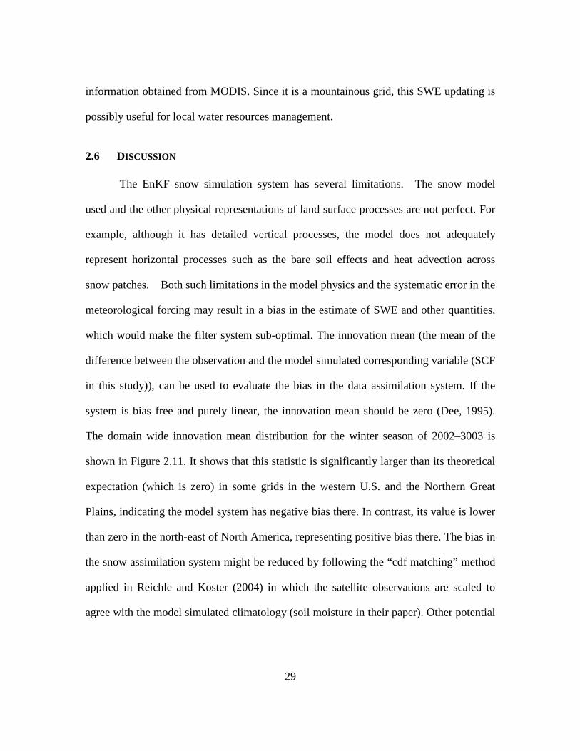
2.6 Discussion ........................................................................................... 29
2.7 Concluding remarks ............................................................................ 31
Chapter 3: Parameter estimation in ensemble based snow data assimilation: a synthetic study ..................................................................... 47
3.1 Abstract ............................................................................................... 47
3.2 Introduction ......................................................................................... 48
3.3 Methodology ....................................................................................... 51
3.4 The performance of parameter estimation with perfect-model-structure53
3.5 Effects of structural error on parameter estimation ............................... 60
3.6 Discussion .............................................................................................. 63
3.6.1 Parameter estimation convergence/divergence .......................... 63
3.6.2 Several limitations in current research ....................................... 65
3.7 Concluding remarks ............................................................................... 66
Chapter 4: Multi-sensor snow data assimilation at continental-scale: the value of GRACE TWS information .......................... 85
4.1 Abstract .................................................................................................. 85
4.2 Introduction ............................................................................................ 86
4.3 Data and methodology ........................................................................... 90
4.3.1. MODIS and GRACE satellite datasets ..................................... 90
4.3.2 Observation based climatologic SWE and snow depth datasets 91
4.3.3 Land surface model .................................................................... 92
4.3.4 The ensemble Kalman filter and smoother ................................ 92
4.4 Implementation of the data assimilation experiments ........................... 95
4.5 Results .................................................................................................... 98
4.5.1 Monthly SWE difference between MOD and MOD_GR .......... 98
4.5.2 Terrestrial water storage anomaly ............................................ 100
4.5.3 Climatologic monthly SWE and snow depth ........................... 102
4.6 Discussion ............................................................................................ 105
4.6.1 Role of the auto-covariance of SWE ensemble ....................... 105
4.6.2 Ensemble variance reduction by assimilating GRACE ........... 107
4.7 Concluding remarks ............................................................................. 108

x
Chapter 5: Conclusions and future work ....................................................... 120
5.1 Summary .............................................................................................. 120
5.2 Future work .......................................................................................... 123
Appendix ............................................................................................................. 127
References ........................................................................................................... 128
Vita ............................................................................................................ 136

xi
List of Tables
Table 2.1 Calibrated parameter α used in observation operator for different land types ........................................................................................................................................... 33
Table 3.1. Description of simulations in experiments. ..................................................... 68
Table 3.2. The Nash-Sutcliffe efficiency for ensemble mean of different simulation shown in Figure 3.1. The value equal to 1 represents the perfect simulation, with the value the larger the better. ................................................................................................. 69
Table 3.3. The temporal averaged error in SWE (ensemble mean minus the true value) for parameter estimation run DA_STRUCT_TRUE with different 0Q shown in Figure
3.8. Here 0Q is represented by standard deviation (0Q ), which is equal to R multiplying
the initial parameter: Std=R*0α . ...................................................................................... 70
Table 3.4. The temporal averaged error in SWE (ensemble mean minus the true value) for parameter estimation run DA_STRUCT_NEW with different 0Q shown in Figure
3.9. Here 0Q is represented by standard deviation (0Q ), which is equal to R
multiplying the initial parameter: Std=R*0α . .................................................................. 71
Table 3.5. The ensemble mean of α retrieved in DA_STRUCT_TRUE when ground is snow-free in May (for every ensemble member), as a function of different 0Q
constraining the parameter variance. Here 0Q is represented by standard deviation
( 0Q ), which is equal to R multiplying the initial parameter: Std=R*0α . ...................... 72
Table 3.6. The dZ retrieved in DA_STRUCT_NEW when ground is snow-free in May
(for every ensemble member), as a function of different 0Q constraining the parameter
variance. Here 0Q is represented by standard deviation (0Q ), which is equal to R
multiplying the initial parameter: Std=R* 0dZ . ................................................................. 73
Table 4.1 The mean absolute error (MAE) of monthly SWE (mm) from Jan to Jun at eight river basins in North America for three experiments. The superscripts represent that

xii
a specific experiment has significantly lower MAE (t-test, p-value < 0.01) in associated river basin and month than some of its counterparts. In particular, (a) - MOD_GR MAE is significantly lower than that of both MOD and Open Loop; (b) - MOD_GR MAE is only significantly lower than MOD; (c) - MOD_GR MAE is only significantly lower than Open Loop; (d)- Open_Loop MAE is significantly lower than that of both MOD and MOD_GR; (e) – Open Loop MAE is only significantly lower than MOD. ................... 110
xiii
List of Figures
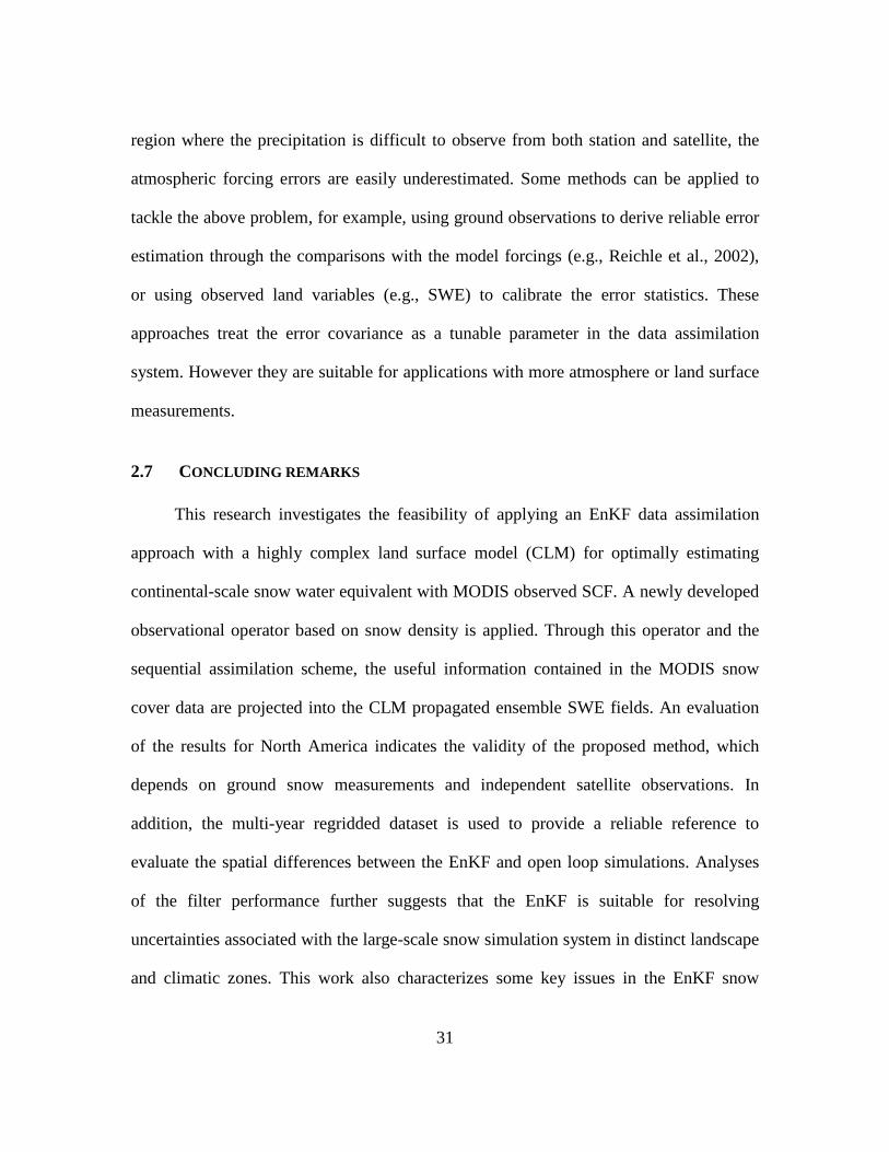
Figure 2.1. SCF parameterization using snow density. Each curve represents a different snow density in equation (6). ............................................................................................ 34
Figure 2.2. Comparison of regional averaged SWE (52º–54 º N, 112º –114ºW , shown as the rectangular box in the upper panel in Figure 2.5, in 2002–2003) from simulation results and ground observations. ....................................................................................... 35
Figure 2.3. Comparisons among daily basin averaged SWE estimations in North Central River Basin. A five-day moving average is used on AMSR-E data to filter out the high frequency fluctuations in the original AMSR-E daily data. ..................................... 36
Figure 2.4. Comparisons among daily basin averaged SWE estimations in the Missouri River Basin. ....................................................................................................................... 37
Figure 2.5. The spatial distribution of the monthly averaged SWE (mm) in Feb from the EnKF and open loop simulations, the climatology from reanalysis dataset, and the AMSR dataset. .............................................................................................................................. 38
Figure 2.6. The spatial distribution of SWE standard deviation (mm) in Feb derived from the reanalysis dataset, the absolute value of monthly mean (Feb) difference (mm) between the EnKF and climatology, also the difference (mm) between the open loop and climatology. ...................................................................................................................... 39
Figure 2.7. Comparison of the EnKF and open loop simulated monthly mean SWE with reanalysis derived climatological mean from Nov, 2002 to Jun, 2003 in three rectangular regions. .............................................................................................................................. 41
Figure 2.8. Ensemble simulations of SWE and their error statistics at a grid in the prairie region. .................................................................................................................... 42
Figure 2.9. Ensemble simulations of SWE and their error statistics at a grid in the boreal forest region. .......................................................................................................... 43
Figure 2.10. Ensemble simulations of SWE and their error statistics at the grid in the mountainous region. .......................................................................................................... 44

xiv
Figure 2.11. Spatial distribution of the average of the innovation (difference between observation and simulation) mean for the winter season in the 2002-2003 simulation (December 2002 to April 2003). ....................................................................................... 45
Figure 2.12. Spatial distribution of the mean of normalized innovation variance (equation (2.7) for the winter season in 2002–2003 (December 2002 to April 2003). ..... 46
Figure 3.1. Ensemble mean simulations of SWE (mm) for SYN_CR, DA_PAR_CR and SYN_TRUE, DA_PAR_α , DA_PAR_θ , DA_TRUE. (see Table 3.1 for the description of these simulations). ........................................................................................................ 74
Figure 3.2. Parameter ensemble mean of α in DA_PAR_α . ................................ 75
Figure 3.3. Parameter ensemble mean of θ in DA_PAR_θ ......................................... 76
Figure 3.4. Ensemble mean of DTR (diurnal temperature range) for SYN_CR, DA_PAR_CR and SYN_TRUE, DA_PAR_α , DA_PAR_θ , DA_TRUE. ................... 77
Figure 3.5. Daily averaged ensemble mean of ground radiative temperature for SYN_CR, DA_PAR_CR and SYN_TRUE, DA_PAR_α , DA_PAR_θ , DA_TRUE. ................... 78
Figure 3.6. Daily averaged ensemble mean sensible heat flux for SYN_CR, DA_PAR_CR and SYN_TRUE, DA_PAR_α , DA_PAR_θ , DA_TRUE. ................... 79
Figure 3.7. Daily averaged ensemble mean albedo for SYN_CR, DA_PAR_CR and SYN_TRUE, DA_PAR_α , DA_PAR_θ , DA_TRUE. .................................................. 80
Figure 3.8. Ensemble mean error in SWE (mean – true value) for DA_STRUCT_TRUE with different 0Q constraining the parameter variance. ................................................ 81
Figure 3.9. Ensemble mean error in SWE (mean – true value) for DA_STRUCT_NEW with different 0Q constraining the parameter variance. ............................................... 82
Figure 3.10. Parameter ensemble mean for DA_STRUCT_TRUE with different 0Q constraining the parameter variance. ................................................................................ 83

xv
Figure 3.11. Parameter ensemble mean for DA_STRUCT_NEW with different 0Q constraining the parameter variance. ................................................................................ 84
Figure 4.1. The difference of monthly SWE (mm) between MOD_GR and MOD data assimilation experiments in the cold season of 2003. ..................................................... 111
Figure 4.2. Eight river basins in North American that are analyzed. .............................. 112
Figure 4.3. The monthly TWS anomaly (Nov, 2002-May, 2007) from the simulations: OL, MOD, MOD_GR and the GRACE observation, averaged over four river basins in North America. In OL, the TWS anomaly in other months in the years of 2002 and 2007 are also shown for reference. .......................................................................................... 113
Figure 4.4. Same as Figure 4.3., but for another four river basins in North America. 114
Figure 4.5. The difference of average Apr SWE (mm) between simulation result (MOD_GR, MOD and OL) and CMC. CMC Apr SWE is given for reference. ............ 115
Figure 4.6. The climatological monthly mean SWE (mm) and snow depth (m) from Nov to Jun in two rectangular regions for the simulations (MOD, MOD_GR and OL), and the CMC long term observation data. Upper panel: (A) 51º–55 º N, 94º –85ºW; Lower panel: (B) 46º– 49º N, 98º –94ºW. See the rectangular boxes in Figure 4.8 for their locations. ......................................................................................................................... 116
Figure 4.8. In those colored grids, the number of the days in which the corresponding daily correlation (zero temporal and spatial lag) between (1) SWE and soil moisture (upper) (2) SWE and groundwater (lower) is significant (p value < 5%) exceeds two in February 2003. ................................................................................................................ 118
Figure 4.9. The daily river basin averaged ρ (%) (equation (4.7)) from Jan to Jun 2003, for the Mackenzie River basin and the North Central River basin. ................................ 119

1
Chapter 1: Introduction
1.1 IMPORTANCE OF LARGE-SCALE SNOWPACK ESTIMATION
Snowpacks are an important component of the Earth’s climate system, serving as
critical freshwater reservoirs and playing a unique role in the global water and energy
cycles. Of all the large-scale (e.g., regional to continental to hemispheric scale) terrestrial
features, snowpacks have the largest fluctuations in space and time, with the area ranging
from 7% to 40% in the Northern Hemisphere during the annual cycle. Associated with
these fluctuations are variations in the surface albedo and radiation balance, turbulent
heat exchange with the atmosphere, water vapor input to the atmosphere through
sublimation and evaporation, and water input to the soil and river systems through melt.
Consequently, an accurate estimation of snow water equivalent (SWE), snow depth, and
other snowpack properties on a large-scale is important for many active research areas,
which include:
(1) Hydrological prediction and water resources management. Much of the global
population (one-sixth, according to Barrett et al., 2005) lives in areas where streamflow is
dominated by snowmelt runoff. Therefore, a reliable description of spatial and temporal
variability of snowpack is critical for the estimation of freshwater availability in those
regions.
(2) Assessment of climate change impacts in cold regions. Global climate change
may have profound impacts on land hydrological processes. However, the impacts on
snowpack variation in large time scales (e.g., inter-annual to decadal scale or larger) are

2
still poorly understood at the global scale, except for some assessments for areas with
abundant snow data (e.g., western U.S. (Mote et al., 2005)).
(3) Characterization of climate-snowpack linkages, as related to atmospheric general
circulation and some low-frequency climate system modes. Continental-scale snow
anomalies can lead to considerable variations in the atmosphere (e.g., Cohen and
Entekhabi 2001; Gong et al., 2002), and in turn can be controlled by atmospheric
temperature and/or general circulation (e.g., Derksen et al., 1997; Clark and Serreze,
2000). Low-frequency climate modes, although largely produced from ocean-atmosphere
interaction, are often seen over land (including snowpack variability). Recent research
(Ge and Gong, 2009) demonstrated a significant relationship between North American
snow depth and the Pacific Decadal Oscillation (PDO) and the Pacific-North American
(PNA) pattern. As highlighted in their work, characterization of these relationships
hinges on a newly available continental-scale snow depth dataset (Dyer and Mote 2006).
In addition to the above mentioned areas, large-scale snowpack information is also
valuable to many other applications, for example, evaluation of coupled Global Climate
Models (GCMs) in terms of their ability to represent observed snow dynamics (e.g., Frei
and Gong, 2005) and the derivation of initial land data for climate and meteorological
numerical simulation (e.g., Souma and Wang, 2009).
1.2 LARGE-SCALE SNOWPACK VARIABILITY MONITORING
Snowpack variability is complex in both temporal and spatial scales. Temporally it
mainly involves accumulation and melting stages. At accumulation stage, the dominant

3
processes include precipitation, sublimation, wind blowing, etc. At melting stage, the
dominant processes include solar radiation, canopy-snow interaction, snow-albedo
feedback, etc. Spatially, the distribution of snowpack can show different patterns across
various scales. For example, at 1~100 meters scale, snow distribution could be controlled
by distributions of leaf area, plant type composition, canopy density (Liston, 2004). At
1~10km scale, snow variability was found (e.g., Donald et al., 1995; Pomeroy et al.,
1998) to follow two-parameter log-normal distribution. Given the general
interchangeability among specific distribution formats by fitting appropriate parameters,
the snow variability at the above scale can be also characterized by other distributions,
such as Poisson or Gamma distribution. In addition, field work (e.g., Shook and Gray,
1996; Deems et al., 2008) demonstrated that snow distribution has fractal property,
indicating consistent driving processes running at multi-scales. The detail fractal feature
can be function of local physiography and vegetation characteristics (Deems et al., 2008).
Currently, the task of monitoring large-scale snowpacks depends on ground (in situ)
and satellite observations. These two approaches are briefly reviewed in this section, with
additional discussion on their limitations (along with the strength of the data assimilation
approach) in next section of this chapter. There are other complementary methods for
snow monitoring, such as low flying aircraft scanning, which are not discussed here
because their data are not used.
1.2.1 Ground measurements
Ground surveys of snowpack properties, including SWE, snow depth, snow density,
and grain size through well designed snow courses and/or operational meteorological

4
stations, is highly accurate compared to other approaches. In North America there are
several ground survey programs that provide long-term snowpack monitoring over large
areas. For example, the Snowpack Telemetry (SNOTEL,
http://www.wcc.nrcs.usda.gov/snow/) is an extensive, automated system that collects
snowpack and related climatic data in the western United States. Installed and maintained
by the Natural Resources Conservation Service (NRCS), SNOTEL includes 730 sites in
11 states (including Alaska), most of which are located in remote high-mountain
watersheds where access is difficult. The data from SNOTEL are delivered in near-real-
time using meteor burst communications technology. Another example is the Canadian
Daily Snow Depth and Snow Water Equivalent Database
(http://www.ccin.ca/datasets/snowcd/docs/1999/DOCUMNTS/INTRO_E.HTM) which
consists of daily ruler measurements of snowpack taken by Meteorological Service of
Canada (CMC) observers. The dataset extends from late 1800s to after 2000, although
most of the data were collected after 1950. At their peak in the early 1980s, there were
over 1700 snow course observations per year in the database. The number of associated
snow course stations sharply declined after 2000.
1.2.2 Satellite observations and inversion
As a promising alternative of ground snow measurements, satellite observations have
been explored by the research community in recent decades. This remotely sensed
information is becoming a major tool for large-scale snow characterization, mainly owing
to its superb spatial coverage (usually at continental to global scale), near-real-time
delivery, and many other cost-effective features.
5
Different physical mechanisms are used by these space-born sensors for monitoring
various features of snowpacks. In particular, the areal extent of snowpack can be detected
and monitored by visible/infrared (VIS/IR) sensors because the reflectivity of snow in
these bands is unique compared with other types of land cover (Hall et al., 2002). The
passive microwave sensors can detect thermal radiation from snow, from which they can
infer snow mass and/or depth (as well as grain size, density and other snowpack internal
properties) information (Derksen et al, 2003; Tedesco et al, 2004; Foster et al, 2005).
Other technologies include active microwave sensing (e.g., Tsang et al., 2007), which can
be used to quantify the areal extent of snowpack.
All these remote sensing approaches consist of some “inversion” algorithms, which
map actual signals obtained at satellites (e.g., electromagnetic fields at ground) to those
variables of interest (e.g., SWE, snow depth). These inversions depend on various
assumptions. Some of these algorithms are relatively simple and straightforward, for
example, the normalized difference of snow index (NDSI) for snow areal retrieval (Hall
et al., 2007), and linear regression of brightness temperature for snow depth retrieval
(Derksen et al, 2003). Other algorithms involve more complicated mechanisms, for
example, using radiative transfer models to derive snow mass and snow depth
information from passive microwave observations (e.g., Tedesco and Kim, 2006). Each
inversion method may have its own strengths and weaknesses, depending on the
geophysical properties of the location where it is applied, and the corresponding
assumptions on which it relies.

6
1.3 SNOW DATA ASSIMILATION
Ground or satellite measurements alone cannot fully meet the need for accurate
characterization of snowpack at large-scale for a number of reasons involved. The value
of in situ observations is constrained by its spatial representativeness, which is usually at
the order of 10~100 m and a function of local topography, vegetation, wind, etc (e.g.,
Liston, 2004). Accordingly, the use of point scale ground measurements to delineate
macro-scale (10~100 km in grid size) snow variability can introduce significant error
(e.g., Pan et al., 2006). Satellite measurements, on the other hand, are usually not a direct
reflection of snowpack hydrological properties. The estimates from inverting satellite
signals can often be contaminated by some unresolved factors, such as the complex
topography, vegetation and meteorological conditions (e.g, clouds). The error associated
with this inversion process can be very complicated, with its magnitude varying from
location to location and from season to season. Before being widely applied in different
climatic and/or hydrological applications, these satellite products need to be
comprehensively evaluated (Foster et al, 2005) regarding their application scope and
error quantification. However, regional to continental evaluation of satellite retrievals can
be very difficult, considering the lack of benchmark data (independent high-quality
observations) at these scales. In addition, the spatial and temporal scales of these satellite
observations could significantly differ from (usually coarser than) those required by
applications because of sensor and orbit limitations.
Given these limitations of in situ and remote sensing snowpack observations, snow
data assimilation has emerged in recent years as an innovative approach (Andreadis and
Lettenmaier, 2006; Clark et al., 2006; Durand and Margulis 2007, 2008). Its goal is to

7
more accurately characterize snowpack variability across a variety of scales. Its central
idea is to combine snow observations with model estimates. Here model refers to the
numerical simulation of snowpack physical processes driven by meteorological forcing.
There are a large number of studies about developing numerical models to estimate
snowpack (Jordan, 1991; Koren, 1999; Niu and Yang, 2004). In general, snow models are
subject to various errors, such as forcing (e.g., precipitation and temperature data) error,
physical parameterization (structural) error, and parameter error. Schemes (e.g., data
assimilation) that optimally integrate models and observations offer promises to reduce
errors in each of them. In its early stage, snow data assimilation used a direct insertion
method (Liston, 1999; Rodell, 2004), which assumes snow observations are perfect.
Recent research recognized that more sophisticated methods are needed to derive weights
that combine models and observations and represent their individual uncertainty, and fit
other requirements such as sequential estimation. The Kalman type algorithms (e.g., the
Kalman filter) and ensemble (Monte Carlo) approaches (ensemble Kalman filter (EnKF),
Evenson, 1994) were introduced to address this need, particularly for the purpose of
accurately representing the temporally and/or spatially varying error statistics of models
and/or observations. In addition, various kinds of ensemble snow data assimilation
schemes have been developed to accommodate distinct properties of different snow
observations (Andreadis and Lettenmaier, 2006; Durand and Margulis 2007). These
include the data from the inversion of the satellite signal, and radiance (both VIS/IR and
microwave) observation directly obtained by satellite.
8
1.4 MOTIVATION FOR DEVELOPING ADVANCED LARGE-SCALE SNOW DATA
ASSIMILATION SCHEMES
In general, the current snow data assimilation schemes are not adequate for large-
scale snowpack estimation. Most previous ensemble snow data assimilation experiments
were designed at watershed or smaller scale, and so many complex issues that could be
critical for large-scale retrieval have been neglected. In particular, the impacts of different
climatic (e.g., temperature and precipitation regime, and wind pattern) and geographical
(e.g., topography, vegetation) conditions on the data assimilation performance are
especially important but not well understood. These impacts can only be explored and
assessed over a large-scale region. Also the robustness of data assimilation algorithms,
such as the observational operator (a function that relates an observation with a model
estimate) and the error parameters in the EnKF, has not been adequately tested in
previous research. The spatial heterogeneity of snowpack and land cover, together with
other complexities involved for a large domain, may impose additional requirements on
these algorithms. Consequently, the development and evaluation of new observational
functions or other components may become necessary.
The motivation for the research in this dissertation not only came from the above
mentioned “large domain” problem, but also from other theoretical and practical
considerations pertinent to snow estimation. In particular, the effects of parameter and
model structural error on snow data assimilation are not discussed in the literature, which
limits the value of proposed algorithms because they often need to be applied in untested
areas where both the true (or most appropriate) model structure and parameters are
unknown. This deficiency can be especially evident in large-scale applications, because

9
the proper parameter (even structure) may be spatially varying and difficult to estimate. It
is necessary to quantify and mitigate the impacts of these errors with some “flow-
dependent” approach (which means running concurrently with model propagation).
Furthermore, my research has been motivated by the fact that only limited satellite
information (single sensor observation) has been considered in traditional large-scale
snow data assimilation studies. There are always drawbacks inherent to any given type of
observation (e.g., Moderate Resolution Imaging Spectroradiometer (MODIS) observed
snow cover fraction (SCF)) and their negative effects (e.g., systematic error) can be
preserved in associated data assimilation products. As advocated in some synthetic
radiance research (e.g., Durand and Margulis 2006, 2007), assimilation of
complementary information from different radiometer sensors or frequencies can mitigate
the problem and lead to better snow estimates. However, these studies focused on
assimilating synthetic radiometer observations (which include the brightness
temperature and/or albedo at microwave and/or VIS/IR bands) at relatively small scale.
One problem is that their effectiveness could be influenced by high standing vegetation
(e.g, forest), as well as the patchy pattern of snow cover because the thermal emission
from vegetation and soil can dominate the radiometer signal (Andreadis et al., 2008). In
this regard a relatively coarse grid (as commonly adopted in large-scale simulations)
blending multiple vegetation types and snow cover/free patches, could affect
performance of these approaches. In addition these multi-frequency algorithms are
complicated by the “many-to-one” problem (the radiometric signal is a function of many
snowpack properties like SWE, snow depth, snow density, grain size, etc). The
estimation of a particular property (e.g., SWE) could be significantly influenced by errors
10
in quantification of others (e.g., grain size) (Andreadis et al., 2008). Although the
snowpack radiative transfer models (RTM) that have been incorporated that can simulate
these properties (and their errors), their ability (e.g., in grain size simulation) to cope with
geographic heterogeneity (e.g., snowpack or vegetation variability) on a large-scale has
not been adequately evaluated in the literature. Another caveat associated with the multi-
frequency algorithms is that microwave bands are generally less effective in estimating
snowpack with liquid water. Novel approaches are needed that can integrate further
complementary observations and accommodate specific features confronted in large-scale
application, and also avoid the problems of multi-frequency radiometer assimilation.
This dissertation is a first attempt to address all the limitations raised above. It
focuses on the scientific question of how to estimate large-scale snowpack properties
accurately through advanced ensemble data assimilation methods and multiple types of
observations. These investigations have not been previously performed, so some “proof-
of-concept” studies are given in this dissertation. In brief, my research in this dissertation
improves on previous work by 1) using a newly developed observational operator for a
North American data assimilation experiment, in which various climatic and geographic
zones are covered and their impacts to the EnKF performance are comprehensively
evaluated; 2) performing simultaneous state and parameter estimation in a synthetic
EnKF framework, and investigating the dependence of parameter estimation on model
structure error is investigated; 3) blending observations from two sensors (measuring
SCF and terrestrial water storage (TWS), respectively) into a North American snow data
assimilation framework that integrates two differing ensemble methods, and factors that

11
can hamper multi-frequency radiometer assimilation are generally circumvented by the
unique features of MODIS and GRACE observations.
1.5 OUTLINE OF THIS DISSERTATION
Chapter 2 presents a continental-scale SWE data assimilation experiment, which
integrates MODIS SCF data with Community Land Model (CLM) estimates via the
EnKF. It uses a newly available observational function, and the performance of data
assimilation is comprehensively evaluated over various climatic and geographical
environments. Chapter 3 provides a group of synthetic EnKF experiments that jointly
estimate state and parameter. It incorporates a parameter estimation scheme and evaluates
its merit for snowpack estimation. Also Chapter 3 provides a preliminary assessment of
the impacts of model structure error on the performance of parameter estimation. Chapter
4 develops a multi-sensor snow data assimilation system over North America. It
integrates both Gravity Recovery and Climate Experiment (GRACE) TWS and MODIS
SCF information into CLM using the ensemble Kalman filter (EnKF) and smoother
(EnKS). Chapter 5 summarizes the major finds, and presents possible directions for
future research.
12
Chapter 2: Enhancing the estimation of continental-scale snow water equivalent by assimilating MODIS snow cover
with the Ensemble Kalman Filter1
2.1 ABSTRACT
SWE datasets at continental-scale are generally not available, although they are
important for climate research. This study investigates the feasibility of a framework for
developing such needed datasets over North America, through the EnKF approach that
assimilates the snow cover fraction observed by the MODIS into the CLM. I use
meteorological forcing from the GLDAS to drive CLM, and apply a snow-density based
observation operator. This new operator is able to fit the observed seasonally varying
relationship between the snow cover fraction and the snow depth. Surface measurements
from Canada and Advanced Microwave Scanning Radiometer-Earth Observing System
(AMSR-E) estimates (in particular regions) are used to evaluate the assimilation results.
The filter performance including its ensemble statistics in different landscapes and
climatic zones is interpreted. Compared to the open loop, the EnKF method more
accurately simulates the seasonal variability of SWE and reduces the uncertainties in the
ensemble spread. Different simulations are also compared with spatially distributed
climatological statistics from a regridded dataset, which shows that the SWE estimates
from the EnKF are most improved in the mountainous West, the Northern Great Plains,
and the West and East Coast regions. However in boreal forest the performance of the
1Substantial portions of this chapter were previously published in Su, H., Z.-L. Yang, G.-Y. Niu, and R. E. Dickinson (2008), Enhancing the estimation of continental-scale snow water equivalent by assimilating MODIS snow cover with the ensemble Kalman filter, J. Geophys. Res., 113, doi:10.1029/2007JD009232. The References section contains full citations for all articles referenced here.

13
EnKF is degraded. Limitations of the assimilation system are analyzed and the domain
wide innovation mean and normalized innovation variance are assessed, yielding
valuable insights (e.g., about the misrepresentation of filter parameters) as to
implementing the EnKF method for the estimation of large-scale snow properties.
2.2 INTRODUCTION
Snow is a very important component of the climate system that controls surface
energy and water balances. Its high albedo, low thermal conductivity, and properties of
surface water storage impact regional to global climate, as has been documented in
numerous observational and modeling studies (e.g., Barnett et al., 1999; Yang et al.,
2001; Gong et al., 2003).
The various properties characterizing snow are highly variable and so have to be
determined as dynamically active components of climate. These include SWE, density,
and SCF. However, on large spatial scales the properties of snow are not easily quantified
either from modeling or observations. For example, station based snow measurements
often lack spatial representativeness, especially in regions where the topography,
vegetation and overlaying atmosphere produce considerable heterogeneity of the
snowpack distribution (Liston, 2004). In recent decades SWE and snow depth products
have been available from passive microwave sensors (e.g., AMSR-E). Nevertheless,
since the microwave signature of snowpack depends on a number of varying features
(e.g., snow grain size, density, liquid water content, vegetation, etc), direct estimation
(e.g., linear regression) of snow parameters that does not include these dynamic
properties can be plagued by complicated errors (Grody et al. 1996; Forster et al., 2005;

14
Dong et al., 2005). In addition, snow estimation from land surface models (LSMs) can
have large uncertainties partly due to their imperfect parameterizations of snow dynamics
and the errors in their meteorological forcing. Since neither observations nor LSMs
alone are capable of providing adequate information about the time space variability of
continental snow properties, it becomes necessary to combine their information as
achievable through the technology of land surface data assimilation (e.g., McLaughlin,
2002; Houser et al., 1998; Reichle et al., 2002; Margulis et al., 2002; Crow et al., 2003).
Such assimilation can effectively reduce estimation uncertainties through optimally
combining the information from both LSMs and observations.
A number of studies have initially applied data assimilation methods for deriving
snow properties (e.g., SWE) (e.g., Rodell and Houser, 2004; Slater and Clark, 2006;
Dong et al., 2007; Durand and Margulis, 2006, 2007). Among these studies the ensemble
Kalman filter (EnKF) has been used to combine the observed SCF information with the
model simulated SWE (e.g., Andreadis and Lettenmaier, 2006; Clark et al., 2006). The
SWE, a prognostic variable derived from the snow mass balance, has been optimally
updated through its correlative relationship with other more readily observed quantities
(e.g., SCF). However, most of these studies were confined to small river basins or plot
scales, and few have addressed continental or hemispheric applications where the snow
effects on the atmospheric circulation may be pronounced and where the simulation and
observational uncertainties of snow properties may depend on different landscape
properties and climate zones. Thus, more optimal methods of estimation on these scales
are needed. Further, only limited (some very simple) snow physical models and
observational functions were involved in previous studies, and the performance of the
15
data assimilation was inadequately evaluated for operational application. Therefore the
feasibility of data assimilation methods for the retrieval of such properties on a large-
scale has not yet been decisively demonstrated.
The purpose of this paper is to assess the feasibility of the EnKF methodology and
a new observational operator for the retrieval of SWE on a continental-scale. It
demonstrates that the SCF as measured by the MODIS instrument can be assimilated into
continental SWE fields simulated by a highly complex LSM - the National Center for
Atmosphere Research (NCAR) CLM. Section 2 gives a brief description of the EnKF,
the CLM, and a recently developed SCF observational operator. Datasets and
experiments are discussed in Section 3. The results analyses are given in Section 4.
Section 5 discusses limitations of the proposed method, with concluding remarks in
Section 6.
2.3 METHODOLOGY
The EnKF based snow data assimilation system used in this paper has two
essential components: (1) an LSM (including its snow model) that evolves related state
variables in an ensemble approach and provides background error statistics; (2) the
Kalman filter updating scheme that combines the physical simulations with observations
using an observational function.
2.3.1 The LSM
The CLM (e.g., Bonan et al., 2002, Oleson et al., 2004) numerically simulates
energy, momentum, and water exchanges between the land surface and the overlying
atmosphere at each computational grid. It employs 10 soil layers to resolve soil moisture
16
and temperature dynamics and uses plant functional types (PFTs) to represent sub-grid
vegetation heterogeneity. The CLM snow model simulates a snowpack with multi-layers
(1-5 layers) depending on its thickness, and accounts for processes such as liquid water
retention, diurnal cycling of thawing–freezing, snow melting, and surface frost and
sublimation. Heat and water are transported between its adjacent snow layers, also
between its top layer and the overlying canopy and/or the atmosphere. Snow layers may
be combined or divided every time step to ensure a realistic representation of snow
physics and numerical stability. The grid averaged albedo is area weighted using a snow
cover fraction. The CLM also explicitly incorporates densification processes (e.g.,
destructive or equitemperature metamorphism, compaction by snow overburden, and
melt metamorphism) following Anderson (1976), for calculating snow density of each
snow layer. This multi-layer approach is found to significantly enhance the simulation
quality, correcting the previously underestimated snow mass and early time of melting
that is obtained in a single layer model (Yang and Niu, 2003).
The SWE propagation equation in the CLM can be summarized as follows:
dtMEPxx ttttt )(1 −−+= − (2.1)
where tx and 1−tx denote the SWE in a sub-grid tile of a grid at time step t and
1−t , respectively. tP represents the solid precipitation provided by measurements, tE
represents the loss of snow due to sublimation and evaporation, and tM represents the
melting of snow. The latter two quantities are calculated from the model. By adding
together layers, the sub-grid tile total SWE can be obtained as:

17
∑+
=
+=1snl
0iiliq,iice,t )w(wx (2.2)
where iicew , and iliqw , denote solid and liquid water mass in layer i , and snl denotes
the number of layers. Each of these terms has its own mass balance equation similar to
(2.1).
2.3.2 The EnKF and its implementation
The EnKF was first introduced by Evensen (1994) as a Monte Carlo approach to
accomplish the Kalman filter updating scheme in numerical modeling systems. It is also
related to the theory of Stochastic Dynamic Prediction (Epstein, 1969). Detailed
descriptions and discussions of this method in various contexts are available in the
literature (e.g., Evensen, 1994, 2003; Reichle et al., 2002; Hamill, 2006).
Using the model physical configuration described in 2.1, the EnKF is
implemented as follows: (a) each sample (ensemble member) of model state variables
is propagated at every time step using prognostic equations like equation (1); these
simulations are driven by perturbed meteorological forcing data (the method of sampling
forcing is introduced in Section 3); (b) each sample of the LSM forecast variables is
updated (e.g., SWE in this study) using Equation (3):
)v)H(x(yKxx it
jti,tt
jti,
'jti, +−+= (2.3)
where 'j
ti,x denotes the filter updated states (e.g., SWE), jti,x the model simulated states,
i the ensemble index, j the tile index in a given grid, ty the observation in that grid
(SCF in this study), and H the observational operator (to be described subsequently).
18
itv is randomly drawn from a Gaussian distribution (with zero mean and the variance
equal to tR as described below) to ensure an adequate spread of the analysis ensemble
members (Burgers et al., 1998).
The tK in Equation (2.3), which is the “Kalman gain”, takes the form of:
1t
Tbt
Tbtt )RH(HPHPK −+= (2.4)
where btP represents the error covariance of simulated ensembles; tR , the error
covariance of observed SCF. The latter is a prescribed value in this study. The model
state jti,x is a sub-grid tile based value, while the observational statistic ty (SCF) is
defined at a grid. The model is compared with observation using )H(x jti, , the
summation of model predicted SCF over all tiles in the specified grid:
∑=
=n
1e
eti,
jti, )h(x)H(x (2.5)
where e loops all the tiles in the grid and )( ,etixh denotes the observational operator at
each tile weighted by the tile area. It should be emphasized that the above
implementation does not directly assimilate SWE measurements nor does it directly
update the CLM simulated SCF. Instead the implementation updates the CLM simulated
SWE with SCF observations, which requires an observation function linking the state
variable SWE and the MODIS observed SCF as described in section 2.3.3.
The updated SWE or 'j
ti,x in Equation (2.3) represents the total snow mass for
the entire snowpack, which must be disaggregated into ice and liquid parts for each of the
layers according to (2.2). A simple rule is designed for this allocation. Snow mass is
19
always added or subtracted in the layers starting from the top, and the ratio between solid
and liquid water components is kept the same after each allocation (this is a simple
assumption, since there is no information about liquid/solid ratio from SCF observation).
The total snow mass and energy are conserved as the layers are separated or combined,
and the procedure follows the existing parameterization in the snow layering scheme
(Oleson et al., 2004). The snow depth in each layer is also updated accordingly. In CLM
the snow density is calculated from the snow water equivalent and snow depth. Therefore
it can be indirectly updated with these two variables.
2.3.3 The Observational operator
A snow depletion curve (SDC) that parameterizes the relationship between
regional averaged SWE and SCF has been used to optimize SWE estimates in recent
ensemble based data assimilation experiments (e.g., Andreadis and Lettenmaier, 2006;
Clark et al., 2006). Its basic philosophy is that the accumulation or ablation of the
unevenly distributed snow determines both SWE and SCF such that both are highly
correlated (Yang et al., 1997; Luce et al., 1999, 2004; Liston, 2004). Accordingly, any
observed SCF information should contribute to the estimation of SWE.
A new SCF parameterization has been developed by Niu and Yang (2007) using
the snowpack density to account for the large-scale depletion pattern and its temporal
variability. This SCF scheme, which is used in this study to transfer observational
information into the CLM, takes the following mathematical form:
))/(5.2
tanh(0
αρρ newsno
sno
z
hSCF= (2.6)

20
where SCF is the fractional snow cover, snoh and 0z are the spatially averaged snow
depth (or rewritten to be a function of SWE and snow density) and the ground roughness
length, respectively. newρ is a prescribed fresh snow density with adjustable values
depending on local conditions. snoρ is the model calculated snow density. The curve
shape parameter α is tunable and assumed to be controlled by several factors including
scale and, hypothetically, the grid-specific physiographic properties.
The snow depth and snow cover relationship (Equation 2.6) differs from any of the
parameterizations reviewed by Liston (2004). Instead of one static curve for the entire
snow season, it provides a family of snow depletion curves with each such curve
representing a non-linear relationship between SCF and snow depth characterized by a
unique value of snowpack density (Figure 2.1). Further, this SCF operator accommodates
the multi-layer structure of CLM snow model by using the layer integrated snow density
in the Equation (6). Niu and Yang (2007) evaluated the validity of this seasonally varying
SCF scheme using long term (1979-1996) ground based data of SWE and snow depth in
North America (Brown et al., 2003) and satellite observed monthly SCF from Advanced
Very High Resolution Radiometer (AVHRR). Equation (6) performs reasonably well in
terms of reconstructing the relationship between SCF and snow depth in large river
basins in North America.
To apply Equation (6) for data assimilation, it is needed to calibrate newρ and α
based on field measurements or other high-quality datasets at hand. This study sets newρ
to 100 kg/m3 (Dingman, 2002) for each grid in the model domain. The value ‘2.5’ in
Equation (2.6) is itself tunable, but it is here assumed to be a constant for simplicity.
21
My experiments use gridded North America snow datasets (1979-1996) (Brown, 2003)
and AVHRR monthly SCF data to calibrate the shape parameter α . The reason to use
the AVHRR SCF dataset is that it covers the same time period as the data in Brown et al.
(2003). These datasets are regridded to 1° by 1° resolution, the resolution used for the off-
line model. An optimal α is obtained by requiring the SCF derived from Equation (6)
to best fit the AVHRR observed SCF in a least mean square error sense. The Genetic
Algorithm (GA) is used to efficiently search for this optimal parameter. I account for
the region-specific variability of α by considering three landscape categories: (1) flat
regions with low standing vegetation (e.g., the prairie in the Northern Great Plains); (2)
flat regions with high standing vegetation (e.g., the boreal forest of Canada) and (3)
mountainous regions (e.g., the Rocky Mountains). This approach to representing
heterogeneity of SDC is comparable to that of Liston (2004), which used a statistical
distribution to characterize SDC and retrieve related parameters (e.g., CV in Liston
(2004)) based on the physiographic properties of a geographic region to represent.
Three regions in North America have been used to represent the above landscape
categories, each large enough to retrieve the optimal value of α . The calibrated α
(using observations from 1979 to 1993) and correlation coefficient between reconstructed
and observed SCF in the validation period (using observations from 1994–1996) are
given in Table 2.1. Table 2.1 shows that α is slightly less than one for the flat and low
vegetation region, greater than two for the flat and high vegetation region, and in between
over mountainous regions.
22
2.4 EXPERIMENTAL SETUP AND DATASETS
My experiments use near surface meteorological forcing variables from the Global
Land Data Assimilation System (GLDAS) at 1º×1º resolution (Rodell et al., 2004) to
drive CLM. The GLDAS forcing data are observationally derived fields including
precipitation, air temperature, air pressure, specific humidity, shortwave and longwave
radiation. The vegetation and soil parameters from finer resolution raw data of CLM2.0
as used in previous studies (Bonan et al., 2002; Niu et al., 2005) are aggregated. CLM is
run from January 2002 to June 2004, spanning the time period during which the MODIS
retrieved SCF is available.
The GLDAS precipitation and temperature fields are perturbed in order to account
for uncertainties in these model inputs to the snow dynamics. The samples of
precipitation forcing are derived by multiplying the GLDAS values by spatially
correlated log-normal random fields (with zero mean and unit variance), as described in
Nijssen and Lettenmaier (2004). The e-folding scale of horizontal error correlations are
assumed to be 1º in latitude/longitude coordinates, to provide the spatial covariance of
forcing uncertainties. The relative error is defined at 50% in the log-normal distribution
approach. Temperature ensembles are produced in the same way, except that typical
normal random fields are applied to mimic true uncertainties, with zero mean and 3ºC
standard deviation. The ensemble size is set to 25, a compromise between computational
affordability in the large land assimilation system and the filter effectiveness. Previous
studies (e.g., Reichle et al., 2002; Andreadis and Lettenmaier, 2006) showed reasonable
performance for the EnKF with this ensemble size.
23
MODIS observed snow cover fraction is assimilated into the CLM. MODIS uses 36
spectral bands to retrieve land surface properties. Its snow mapping algorithm detects
land snow fraction using NDSI (Hall et al., 1995), and has the ability to distinguish
between snow and cloud (Hall et al., 2002). The spatial resolution of SCF data from
MODIS can be as high as 500 m but the product applied in this research is MOD10C1
with 0.05º resolution (Hall et al., 2002). I determine from the 0.05º cells, a weighted
average at 1º resolution using the CMG confidence indices (Hall et al., 2002), assuming
that the raw data SCF is unchanged by cloud obscuration. A threshold of 50% for the
cloud cover is used to determine whether or not the SCF observation is used in the
corresponding grid. This value is reasonable in that it does not have large negative effects
on the filter performance compared to a stricter criteria, while rendering the system a
relative increase in the SCF data frequency. The model is spun up to November 2002,
and after that the MODIS SCF data sets are assimilated.
The MODIS SCF has errors whose standard deviation varies seasonally and
geographically. Accurate characterization of the MODIS SCF error structure is beyond
the scope of this study. An extensive literature search (e.g., Klein and Barnett, 2003;
Simic et al., 2004; Brubaker et al., 2005; Hall and Riggs, 2007) indicates that it is fairly
reasonable to assume the MODIS error at 10% in this particular study. Using this simple,
stationary error criteria is also consistent with previous research (e.g., Andreadis and
Lettenmaier, 2006). To account for parameter errors, a Gaussian error distribution with
zero mean and 10% (based on nominal value in Table 1) standard deviation is prescribed
for α in Equation (2.6).

24
High-quality, spatially distributed ground SWE data at the continental-scale are
generally not available as independent datasets for validation. Furthermore, since the
snow density is simulated to be a time-dependent variable as considered in Equation 2.6,
the abundant measurements of snow depth across North America (e.g., the NOAA Coop
measurements) may not be directly applied as a benchmark for evaluating the SWE.
Another limitation is the requirement that GLDAS forcing data overlap with MODIS
observations, precluding their use for long-term simulations.
Based on these considerations, two independent observational sources are used
to evaluate the assimilated continental-scale SWE fields. The first source is the ground
measurements in Canada (Canadian Snow CD, 2000) which contain snow course
surveyed SWE data over recent decades. The Canada snow course data are mainly
located in river basins in southern Canada (Canadian Snow CD, 2000; Brown et al.,
2003) encompassing different topographic and vegetative types. The measurements from
winter 2002 to summer 2003 (overlapping with the CLM integration period) are scattered
in western mountainous regions and southern flat regions, with a relatively small portion
of area in the central southern prairie region. The other source is AMSR-E derived SWE
data. AMSR-E (flown on board the NASA Aqua satellite) is a passive microwave
radiometer with a wide range of frequencies (from 6.9–89 GHz), which can provide
spatially and temporally continuous SWE estimation with adequate resolution for global
analyses. These SWE estimates may have large errors in mountainous regions, forests,
and where the snow is wet (e.g., Dong et al., 2005; Foster et al., 2005). Under certain
circumstances (e.g., for low vegetation flat regions where snow is dry and shallow) the
snow grain size and snow density assumed in the retrieval algorithm are relatively

25
reliable (e.g., the Northern Great Plains), the passive microwave retrieved SWE can be
relatively accurate (Brubaker et al., 2001; Mote et al., 2003; Foster et al., 2005).
2.5 RESULTS
2.5.1 Initial evaluation of the assimilated SWE dataset
2.5.1.1 Comparison with ground observations
Distributed observations in the Canadian prairie region are limited, but they are
still suitable for my evaluation. Figure 2.2 shows the inter-station averaged measurements
and their simulation counterparts within the region of 52º–54ºN, 112º–114º in the 2002–
2003 cold season. This comparison is rather representative in my assessing the
assimilation quality for several reasons. First, it illustrates the relatively low frequency of
ground observations, though the accumulation and melting stages are clearly displayed.
Second, it represents some typical benefits through incorporating the SCF information
into the CLM simulation in broad prairie regions. Figure 2.2 shows that the assimilated
SWE values at the peak and melting stage are elevated to value closer to the observations.
The extent to which the SWE is adjusted changes from place to place, determined by the
weighting of model forecasted SCF and MODIS observed SCF according to the ensemble
error statistics. In this particular case, the CLM predicted SCF is lower than that from the
MODIS observations, and the filter partially corrected this difference during the
assimilation cycles. Although only limited ground validation are provided here, it is
argued that these analyses are consistent with the purpose in current research, which is to
obtain a qualitative assessment on the proposed methodology.

26
2.5.1.2 Comparison with passive microwave sensor retrieved data in selected regions
Global SWE estimates from AMSR-E are available for the period of the CLM
simulations in selected regions in North America. In the mid-latitude flat and low
vegetation covered regions with a shallow snowpack, such as the Missouri River Basin
and the North Central River Basin in the Northern Great Plains, AMSR-E derived daily
SWE products can be utilized for assessing assimilation results. The comparisons are
shown in Figure 2.3 and Figure 2.4. In each plot the daily time series of basin averaged
snow water equivalent estimates are displayed, representing the EnKF assimilation run,
the open-loop run (without assimilation) and the AMSR-E estimation, respectively. The
figures indicate that the SCF assimilation significantly adjusts the snow estimation in
these two basins and provides results more like the AMSR-E estimates. During
December to February when the snow is likely to be dry in those regions, the AMSR-E
retrieved SWE should have less uncertainty induced by liquid water content (Tedesco et
al., 2006). During this time, the EnKF simulations better agree with satellite observations
than over the melting period of March and April. Some new snow retrieval algorithms
are currently under development for more accurately inverting or assimilating the passive
microwave signals (e.g., Markus et al., 2006; Durand and Margulis, 2006). The above
results may be further evaluated when those enhanced SWE estimations from space-
borne sensors are available.
2.5.1.3 Spatial patterns evaluation
A ground based SWE regridded dataset from Brown et al. (2003) is used to
further assess the distribution of EnKF assimilated SWE. Its climatological monthly
27
mean values and the associated anomalies facilitate us to interpret the difference between
the model above (open loop) and EnKF simulations. Figure 2.5 shows the spatial
distribution of monthly mean SWE (Feb, 2003) from different simulations, also the
climatological mean (comparisons in other months have similar results). It is clear that in
many regions the EnKF results and the climatology are more similar to each other than
with the open loop, particularly in the Northern Great Plains, the middle-west
mountainous regions, west coastal regions, and part of the east costal regions. However,
the EnKF simulation has a high bias in the boreal forests, which may reflect the forest
effects on MODIS SCF data, or the systematic error in the meteorological forcing.
Figure 2.6 shows the climatological standard deviation of SWE (Feb) as derived
from the multi-year reanalysis dataset, and the absolute difference between each
simulation (Feb, 2003) and the climatology. It demonstrates that in most of the regions
where the EnKF and the climatology are in better agreement, their differences are within
the range of inter-annual variability. Figure 2.7 further supports this conclusion using a
temporal comparison of monthly mean SWE (from Nov, 2002 to Jun, 2003) in three
small representative places within those regions summarized above. The error bars
associated with the climatological mean denotes the standard deviations of monthly
SWE. During the majority of the snow season (e.g., from Jan to Mar), the EnKF
simulated monthly mean values are usually confined within the error bar. In contrast, the
open loop simulations are often outside of the standard deviation range. Specifically in
the first region (41º–42 º N, 75º –80ºW) the difference between the open loop and the
mean is nearly twice a standard deviation, which suggests the erroneousness of the open
loop simulation there. The above spatial evaluation takes an indirect approach because

28
the multi-year data used to construct climatological statistics do not cover my simulation
periods. However, it should be meaningful, partly because of the relative stability of
climatological mean and standard deviation of large-scale SWE.
2.5.2 Assessing the behavior of ensemble filtering in large-scale snow assimilation
The ensemble simulations of SWE at the CLM grid test sites with different land
surface properties and climatic scenarios are presented in Figures 2.8, 2.9, 2.10. Figure
2.8 shows by the middle-latitude prairie grid that the model simulations have large
spreads in both accumulation and melting periods. This variability is markedly reduced in
the data assimilation run, especially in the melting season. Apparently, the GLDAS
forcing terms do not fully constrain the timing of melting compared to the EnKF.
Meanwhile the decrease in the EnKF ensemble variance demonstrates that the EnKF
algorithm is implemented properly in this simulation.
Typical simulation results in boreal forest regions are shown in Figure 2.9. Similar
to those displayed in Figure 2.8, the ensemble uncertainties are reduced in the EnKF run.
However, the effect of altering the peak SWE is not as significant as that shown in Figure
2.8. These areas are covered by large extent of snow of a longer duration than that of the
prairie regions (where the snow cover is usually ephemeral), so it is easier for the model
simulated SCF to agree with MODIS observation, making the filter update more smooth.
The filter feature for a mountainous grid in Colorado (Figure 2.10) appears to be
similar to those in Figures 2.8 and 2.9. However, it differs from the other two in that the
timing of snow melt is largely altered in the EnKF simulation due to the incremental
29
information obtained from MODIS. Since it is a mountainous grid, this SWE updating is
possibly useful for local water resources management.
2.6 DISCUSSION
The EnKF snow simulation system has several limitations. The snow model
used and the other physical representations of land surface processes are not perfect. For
example, although it has detailed vertical processes, the model does not adequately
represent horizontal processes such as the bare soil effects and heat advection across
snow patches. Both such limitations in the model physics and the systematic error in the
meteorological forcing may result in a bias in the estimate of SWE and other quantities,
which would make the filter system sub-optimal. The innovation mean (the mean of the
difference between the observation and the model simulated corresponding variable (SCF
in this study)), can be used to evaluate the bias in the data assimilation system. If the
system is bias free and purely linear, the innovation mean should be zero (Dee, 1995).
The domain wide innovation mean distribution for the winter season of 2002–3003 is
shown in Figure 2.11. It shows that this statistic is significantly larger than its theoretical
expectation (which is zero) in some grids in the western U.S. and the Northern Great
Plains, indicating the model system has negative bias there. In contrast, its value is lower
than zero in the north-east of North America, representing positive bias there. The bias in
the snow assimilation system might be reduced by following the “cdf matching” method
applied in Reichle and Koster (2004) in which the satellite observations are scaled to
agree with the model simulated climatology (soil moisture in their paper). Other potential

30
approaches may include enhanced representation of model parameters and structures
(system identification) in the data assimilation framework.
Determining the covariance of forcing errors is another important issue in land
data assimilation systems (Reichle and Koster, 2003; Crow and Loon, 2006). The forcing
error variances largely dictate the ensemble evolving path and the magnitude of the EnKF
updates. The mean of normalized innovation variance can be used to detect the
misrepresentation of model error in the data assimilation system, as defined below:
]RHHP
vvE[
tTb
t
T
+=ϕ (2.7)
where ν represents the average of innovation over the ensemble members, and []E
represents the temporal mean.
If the EnKF is used with optimal statistical conditions (e.g., linear models and
observational operators, and additive Gaussian errors), and the model errors are perfectly
represented by the ensemble statistics, then the mean of the normalized variance of the
innovation should =1.0 (Dee, 1995). The spatial distribution of the mean of the
normalized innovation variance for the winter season in 2002–2003 is shown in Figure
2.12. Its value is significantly larger than this theoretical expectation in some grids in the
western U.S., the North Great Plains and the eastern coastal regions, but is lower than one
in the northern tundra area. The prescribed forcing errors may be underestimated in the
regions where this statistic is larger than one, while in the regions where this statistic is
lower than 1.0, the forcing errors may be overestimated. This implication is intuitively
reasonable considering that in the middle latitude region where the ground temperature
often fluctuates around the freezing point in the cold season, and in the mountainous
31
region where the precipitation is difficult to observe from both station and satellite, the
atmospheric forcing errors are easily underestimated. Some methods can be applied to
tackle the above problem, for example, using ground observations to derive reliable error
estimation through the comparisons with the model forcings (e.g., Reichle et al., 2002),
or using observed land variables (e.g., SWE) to calibrate the error statistics. These
approaches treat the error covariance as a tunable parameter in the data assimilation
system. However they are suitable for applications with more atmosphere or land surface
measurements.
2.7 CONCLUDING REMARKS
This research investigates the feasibility of applying an EnKF data assimilation
approach with a highly complex land surface model (CLM) for optimally estimating
continental-scale snow water equivalent with MODIS observed SCF. A newly developed
observational operator based on snow density is applied. Through this operator and the
sequential assimilation scheme, the useful information contained in the MODIS snow
cover data are projected into the CLM propagated ensemble SWE fields. An evaluation
of the results for North America indicates the validity of the proposed method, which
depends on ground snow measurements and independent satellite observations. In
addition, the multi-year regridded dataset is used to provide a reliable reference to
evaluate the spatial differences between the EnKF and open loop simulations. Analyses
of the filter performance further suggests that the EnKF is suitable for resolving
uncertainties associated with the large-scale snow simulation system in distinct landscape
and climatic zones. This work also characterizes some key issues in the EnKF snow

32
estimation framework, such as the system bias and model error misrepresentation. It
provides the spatial distributions of related statistics useful for characterizing the quality
of the data assimilation system. The method could be improved by better quantification
of the errors in the modeling system including its mean value (bias) and variance.

33
Table 2.1 Calibrated parameter α used in observation operator for different land types
Flat and Low Vegetation
Mountainous region Flat and high vegetation
Optimized α 0.98 1.69 2.21
Correlation Coefficient R 0.92 0.82 0.96
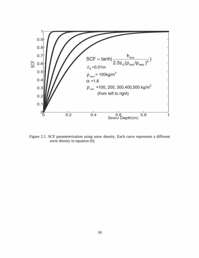
34
Figure 2.1. SCF parameterization using snow density. Each curve represents a different snow density in equation (6).
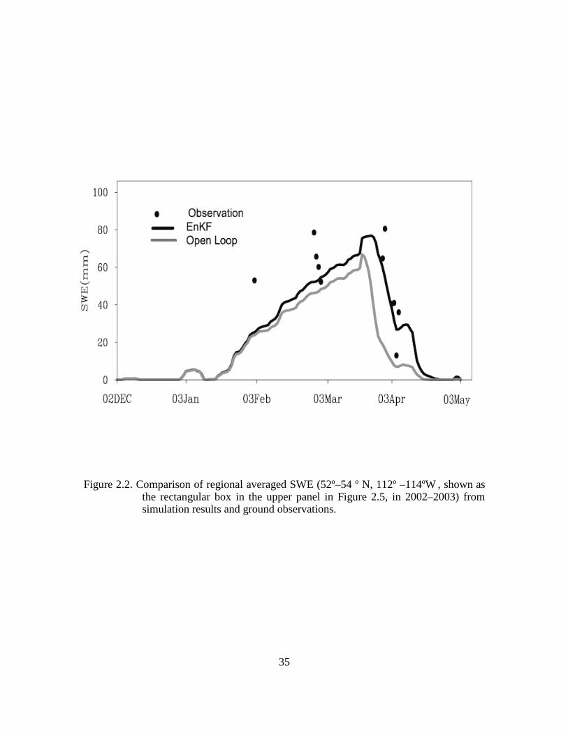
35
Figure 2.2. Comparison of regional averaged SWE (52º–54 º N, 112º –114ºW , shown as the rectangular box in the upper panel in Figure 2.5, in 2002–2003) from simulation results and ground observations.
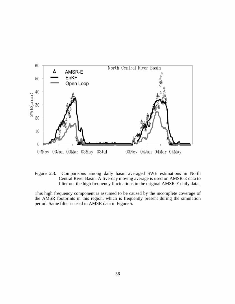
36
Figure 2.3. Comparisons among daily basin averaged SWE estimations in North Central River Basin. A five-day moving average is used on AMSR-E data to filter out the high frequency fluctuations in the original AMSR-E daily data.
This high frequency component is assumed to be caused by the incomplete coverage of the AMSR footprints in this region, which is frequently present during the simulation period. Same filter is used in AMSR data in Figure 5.

37
Figure 2.4. Comparisons among daily basin averaged SWE estimations in the Missouri River Basin.

38
Figure 2.5. The spatial distribution of the monthly averaged SWE (mm) in Feb from the EnKF and open loop simulations, the climatology from reanalysis dataset, and the AMSR dataset.
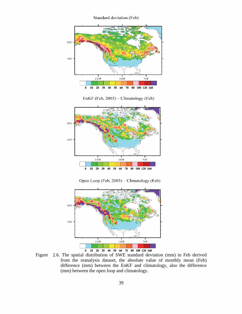
39
Figure 2.6. The spatial distribution of SWE standard deviation (mm) in Feb derived from the reanalysis dataset, the absolute value of monthly mean (Feb) difference (mm) between the EnKF and climatology, also the difference (mm) between the open loop and climatology.
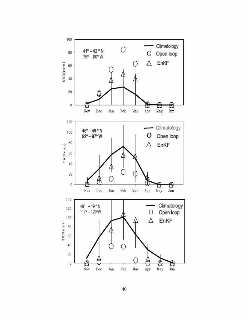
40

41
Figure 2.7. Comparison of the EnKF and open loop simulated monthly mean SWE with reanalysis derived climatological mean from Nov, 2002 to Jun, 2003 in three rectangular regions.
The error bar (vertical line) is given for each climatological mean value, which stands for the standard deviation (inter-annual variability) of each month.

42
Figure 2.8. Ensemble simulations of SWE and their error statistics at a grid in the prairie region.
Left : Open loop run; right: EnKF run. Upper: 2002-2003; Lower: 2003-2004. Ensemble simulations are represented by gray curves, the range (difference between the maximal ensemble value and the minimal ensemble value) of ensemble is the blue curve, and the standard deviation of ensemble is the green curve.

43
Figure 2.9. Ensemble simulations of SWE and their error statistics at a grid in the boreal forest region.
Left : Open loop run; right: EnKF run. Upper: 2002-2003; Lower: 2003-2004. Ensemble simulations are represented by gray curves, the range (difference between the maximal ensemble value and the minimal ensemble value) of ensemble is the blue curve, and the standard deviation of ensemble is the green curve.
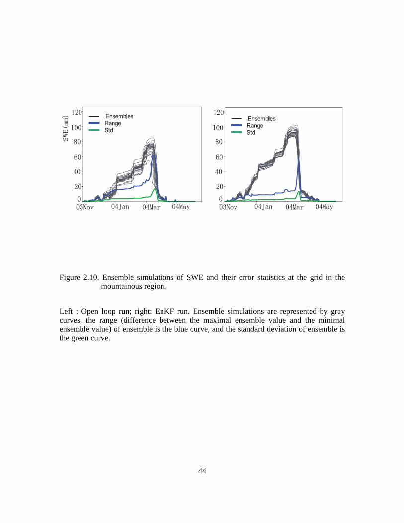
44
Figure 2.10. Ensemble simulations of SWE and their error statistics at the grid in the mountainous region.
Left : Open loop run; right: EnKF run. Ensemble simulations are represented by gray curves, the range (difference between the maximal ensemble value and the minimal ensemble value) of ensemble is the blue curve, and the standard deviation of ensemble is the green curve.

45
Figure 2.11. Spatial distribution of the average of the innovation (difference between observation and simulation) mean for the winter season in the 2002-2003 simulation (December 2002 to April 2003).
This value is significantly larger than its theoretical expectation, zero, in some grids in the western U.S. and the North Great Plains, indicating the model system has low bias there. In contrast, the value is lower than zero in the north-east of North America, representing the model system has high bias there.

46
Figure 2.12. Spatial distribution of the mean of normalized innovation variance (equation (2.7) for the winter season in 2002–2003 (December 2002 to April 2003).
This value is significantly larger than its theoretical expectation, one, in some grids in the western U.S., the North Great Plains and the eastern coastal regions. In contrast, the value is lower than one in the northern tundra area.

47
Chapter 3: Parameter estimation in ensemble based snow data assimilation: a synthetic study
3.1 ABSTRACT
Estimating erroneous parameters in ensemble-based snow data assimilation
systems has received little attention in the literature. The objective of this study is to
assess the effectiveness, performance, and sensitivity of the ensemble based method to
other sources of error such as model structural error. Synthetic one-dimensional snow
data assimilation with the ensemble Kalman filter was run to achieve this obejctive. The
traditional Kalman analysis equation is augmented to include a parameter vector. The
first part of the paper investigates the effectiveness of this parameter estimation approach
in a perfect-model-structure scenario, and the second part focuses on its dependence on
model structure by introducing a simple parameterization error.
Results from first part research show that this parameter estimation approach
reduces the systematic error of SWE estimates, and retrieves the correct parameter value.
In addition, the simulation of related ground energy variables was improved due to
correction of parameters and their influence through model physics. Results from the
second part indicate that, at least in this experiment, there is an evident dependence of
parameter search convergence on model structural error. In the imperfect-model-structure
run, the parameter search diverges, although it can simulate the state variable well.
Empowered by the state-space infrastructure of the EnKF, this result suggests that, good
data assimilation performance in estimating state variables is not a sufficient indicator of
reliable parameter retrieval in the presence of model structural error (here I have good
performance along with parameter divergence). The generality of this conclusion needs to
48
be tested by data assimilation experiments with more complex structural error
configurations.
3.2 INTRODUCTION
As an important freshwater resource, snow also affects the land surface energy
balance via its unique thermodynamic properties (e.g., high albedo, low thermal
conductivity) that vary spatially and temporally. In this respect accurately characterizing
snow conditions is critical for hydrological forecasts, diagnosing hydroclimatologic
trends (Brown et al., 2003) and subsystem interactions (e,g, land snow cover-atmosphere
interaction), and monitoring floods and droughts, among other applications. Although
this need of snow data is pressing, the related tasks of snow monitoring have not been
satisfactorily accomplished over a wide range of scales (e.g., from the watershed-scale
snowpack monitoring to global-scale snow mapping). One difficulty involved in this data
inadequacy is a cold environment that prohibits extensive ground survey efforts.
Remotely sensed snow information provides a new opportunities for snow
estimation. The EnKF methods have been used with such datasets to estimate snow water
equivalent (SWE) and other cold region variables (e.g., Clark et al., 2006; Durand and
Margulis, 2007; Su et al., 2008). The various work focused on different spatial scales,
while they used the same error-covariance based algorithm to sequentially adjust model
simulations. Theoretically, the EnKF method requires that the function relating
observations and model simulations is free of systematic error, to accurately propagate
the ensemble and to avoid bias in the update equation. However, land surface model
(LSM) and observational functions applied in the above studies may have system errors

49
that originate from a broad range of sources including, for example, incomplete
representation of snow properties and associated dynamical processes, uncertainties in
model parameters, and scaling or physical discrepancy (Blöschl, 1999) between
observation and model estimates of snow properties, etc. Each of the related sources of
error is linked to different stages of model development or remote sensing data
processing. The mixture of these errors in the highly non-linear LSM simulation makes
their individual effects difficult to isolate and interpret (Clark et al., 2008). Affected by
these uncertainties, the snow data assimilation system is vulnerable to systematic error
and unrealistic updates, especially in estimating the ensemble mean. In particular,
parametric errors are common in LSMs and observational functions, yielding negative
effects on the EnKF algorithm. Because of the nonlinear nature of the hydrological
system, these effects may be magnified through interactions with other error sources (Liu
and Gupta, 2007).
To tackle such issues, recent studies (Andreadis et al., 2007) have examined the
impacts of parameter uncertainty in multi-scale snow simulations that include its
electromagnetic signatures. However, few studies have focused on methods to correct
parameter uncertainty in ensemble snow data assimilation systems. In most of the EnKF
experiments, critical parameters characterizing snowpack dynamics were simply treated
as perfectly known or by inflating with prescribed noise (e.g., Andreadis et al., 2006; Su
et al., 2008). Related studies in meteorology (Anderson, 2001, Aksoy et al., 2006) have
shed light on how to deal with this drawback. Their work combined parameters and states
in an “augmented vector” and reduced the parameter-state optimization to a state-variable
filtering problem. Following the same general method, this study concentrates on

50
reducing parameter uncertainties in a highly-nonlinear and dissipative snow model forced
with prescribed meteorological data.
Besides its overall performance, another inherently related question is that how
state-space based parameter estimation is dependent on model physical structures (or, the
physical structural error in the system). This issue has often been neglected in previous
research. In other words, it is currently not clear that whether the parameter estimation
algorithm can achieve performance comparable to those using perfect-structure model in
simulating snowpack state variables and retrieve reliable parameter values, given that the
model has structural error. The insights gained from addressing this question may benefit
snow data assimilation in a broad sense. Currently there are a wide range of physical
structures (parameterizations) in different snow models (e.g., Etchevers, et al., 2002),
reflecting distinct (or incompatible) perspectives that represent the same real world
process. These different perspectives usually result from, for example, limited predicative
capability for a given model structure and availability and quality of measurements.
Although it is difficult to rank the physical appropriateness of these model structures, and
each model structure (describing physically equivalent processes) may only capture part
of the truth, understanding the impact of their differences on the parameter estimation
performance in the EnKF environment is crucial to model selection in snow data
assimilation. Further, according to Clark et al (2008), for streamflow simulation in a
given climate regime, selection of model structure could be just as important as selection
of model parameters. This brought upon the similar concern for my research, which is,
can parameter estimation, if conducted elaborately, fully compensate for the structural
deficiency in the EnKF snow estimation system. Insights obtained from this study might
51
contribute to accurately evaluating the cross-region transferability of those estimated
parameters for individual model structure given that true (or most appropriate) structures
and parameters are often unknown (or partially known) for the tested region.
This paper consists of two-fold research that are closely related to each other and
can be accomplished in a common data assimilation framework. First, performance of
parameter estimation in a synthetic EnKF snow data assimilation system is
comprehensively evaluated. In this part the model physical structure is assumed perfectly
known. Built on the similar data assimilation infrastructure, a relatively simple model
structure error is introduced in the second part and performance of parameter estimation
is compared to that of the perfect-model-structure run. The next section introduces the
LSM, the EnKF method, and the parameter estimation scheme. Two different snow data
assimilation experiments are described in sections 3 and 4. A further discussion of results
is given in section 5 with concluding remarks in section 6.
3.3 METHODOLOGY
The CLM (2.0 version, Bonan et al., 2002) is used to propagate land state
variables. CLM numerically simulates energy, momentum and water exchanges between
the land surface and the overlying atmosphere. It employs 10 soil layers to resolve soil
moisture and temperature dynamics and uses plant functional types (PFTs) to represent
sub-grid vegetation heterogeneity. Its snow model simulates a snowpack with multi-
layers (1-5 layers) depending on its thickness, and accounts for processes such as liquid
water retention, diurnal cycling of thawing–freezing, snowpack densification, snow
melting, and surface frost and sublimation. Besides these features, the CLM used in this
52
research includes a new SCF parameterization which dynamically adjust the relationship
between grid averaged SWE and SCF (Niu and Yang, 2007). Estimating a related
parameter in this parameterization is one of the central topics in this experiment. More
discussion about this parameter and the associated equation is given in section 3. The
general performance of CLM2.0 in cold region simulations is given by Bonan et al.
(2002), and Niu and Yang (2006, 2007).
The classic EnKF method (Evensen, 1994) is implemented with an observation
perturbing scheme (Burgers et al., 1998). Additional discussion of the EnKF scheme in
CLM is given by Su et al. (2008). Modifications to include parameter estimation are
incorporated in the same mathematical framework. Equation (3.1) gives a brief statement
of the parameters-augmented EnKF analysis.
))],([()],([)],([ bTttt
bTt
aTt xHyKxx δδδ −+= (3.1)
where tx and δ are state and parameter vectors, all of which are in an ensemble
form; tK , ty and H are the Kalman gain, observations, and observation operator,
respectively. Superscripts a and b denote analysis and background, respectively. To
deal with the problems of variance reduction in parameter ensemble space and filter
divergence, this research adopt the “conditional covariance inflation” method proposed
by Aksoy et al. (2006), which prescribes a threshold for the parameter ensemble variance,
without augmenting ensemble spread at each system propagation step. Equation (3.2)
gives the formulation of this inflation method (which is the evolution equation of
parameter ensemble δ ).
at
bt δδ =+1 if 0)( QVar a
t ≥δ
53
εδδ +=+
at
bt 1 if 0)( QVar a
t ≤δ , ))(,0( 0atVarQN δε −∈ (3.2)
In which ))(,0( 0atVarQN δ− represents the normal distribution with zero mean and
variance of )(0atVarQ δ− . 0Q is the prescribed variance threshold. This inflation
approach has been shown successful in a highly non-linear and flow-dependent
meteorological data assimilation system (Aksoy et al. 2006), where the proper constraints
on parameter ensemble variance are shown to be important for the accurate EnKF update.
Because there is no prior knowledge about the evolution of parameters, 0Q largely
controls the parameter ensemble trajectory. The selection of 0Q and its implications are
discussed in following sections.
3.4 THE PERFORMANCE OF PARAMETER ESTIMATION WITH PERFECT-MODEL-
STRUCTURE
The first group of simulations is synthetic experiment in which a single grid
simulation for six months (November-April) is created with CLM driven by ensemble
meteorological forcing. In the experiment, the true state of related variables is known.
Table 1 provides a list of these simulations. The model time step is 30 minutes, which is
small enough to characterize those major snowpack dynamic processes. For simplicity,
only one vegetation tile type (grass) is used in the grid. Therefore the parameters
involved in the forest-snowpack thermodynamic interactions (e.g., as shown in Niu and
Yang, 2004) are neglected. In addition, the subgrid snow cover heterogeneity is included.
Since the patch of snow cover can drive similar process across a diverse range of scales
in influencing snowpack radiative energy balance, the related experiments in this one-

54
dimensional synthetic study can have some degree of spatial representativeness.
Ensemble forcing is produced by perturbing nominal precipitation and air temperature
with 50% and 3o C (rms) Gaussian error, respectively. The ensemble runs contain 59
members and an additional run is conducted to represent synthetic truth. This provides a
benchmark for quantitatively understanding parameter estimation effects. Synthetic SWE
observations are produced every two days by adding Gaussian perturbations (20 mm rms)
to the true state.
Here consider estimation of two parameters that are typically difficult to determine
from measurements. These are: (1) exponent α in the snow cover fraction
parameterization described by equation (3) (Niu and Yang, 2007); (2) liquid water
holding capacity θ (the maximum volume, in percentage, of liquid water in snowpack,
equation 5). The parameter α governs the relationship between the snow depth (or
SWE) and the snow cover fraction (SCF), strongly influencing grid averaged albedo and
snowpack energy processes (equation (4)). Niu and Yang (2007) have demonstrated the
significant sensitivity of CLM performance in simulating cold region variables to this
parameterization (3) and the parameter α , implying their potential importance to the
snow data assimilation.
))/(5.2
tanh(0
αρρ newsno
sno
z
hSCF= (3.3)
)1(** SCFASCFAA grasssnowtotal −−= (3.4)
θθθ −= −snowpackliquiddrainage , if θθ >−snowpackliquid (3.5)

55
Here snoh and 0z are the snow depth and the ground surface roughness length,
respectively; newρ is a prescribed fresh snow density; snoρ is the model calculated
snow density (Niu and Yang, 2007). totalA is the grid averaged albedo to calculate the
ground energy balance, snowA and grassA are the snow and grass albedo, respectively
(with snowA much larger thangrassA ). With other conditions unchanged, increasing α
generally leads to a decrease of SWE and vice versa. The parameter θ sets the
threshold for the variability of liquid water content in the snowpack, thus controlling its
thermodynamic properties, stratigraphic characteristics (e.g., snow density), and melting
process. With other conditions unchanged, increasing θ generally leads to an increase
of SWE, and vice versa. In previous research (e.g., Niu and Yang, 2007), this parameter
is often given an empirical number without quantitative method to derive application
specific value. The main reason could be that there are few physical laws, if any, to
estimate θ . It can exert significant effects on the dynamical processes. In section 3.3, it
would be shown how an erroneous θ can influence the simulation of snowpack.
A further reason to select these parameters is that I assume they are representative for
the parametric uncertainty in this nonlinear model structure, and the demonstrated system
behaviors could be typical in the scope defined by my central objectives in section 3.1.
Considering that my purpose here is to preliminarily assess the overall performance of
the parameter estimation approach and not to enumerate parameters in different
components of the model and comprehensively characterize their joint estimation,
increasing the number of analyzed parameters may be less important than the need of
keeping the system tractable by limiting the size of parameter vector. Accordingly, the
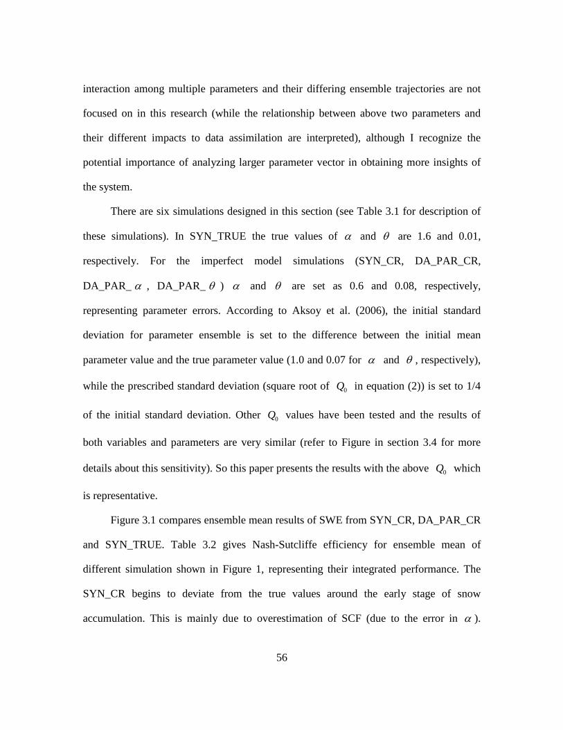
56
interaction among multiple parameters and their differing ensemble trajectories are not
focused on in this research (while the relationship between above two parameters and
their different impacts to data assimilation are interpreted), although I recognize the
potential importance of analyzing larger parameter vector in obtaining more insights of
the system.
There are six simulations designed in this section (see Table 3.1 for description of
these simulations). In SYN_TRUE the true values of α and θ are 1.6 and 0.01,
respectively. For the imperfect model simulations (SYN_CR, DA_PAR_CR,
DA_PAR_α , DA_PAR_θ ) α and θ are set as 0.6 and 0.08, respectively,
representing parameter errors. According to Aksoy et al. (2006), the initial standard
deviation for parameter ensemble is set to the difference between the initial mean
parameter value and the true parameter value (1.0 and 0.07 for α and θ , respectively),
while the prescribed standard deviation (square root of 0Q in equation (2)) is set to 1/4
of the initial standard deviation. Other 0Q values have been tested and the results of
both variables and parameters are very similar (refer to Figure in section 3.4 for more
details about this sensitivity). So this paper presents the results with the above 0Q which
is representative.
Figure 3.1 compares ensemble mean results of SWE from SYN_CR, DA_PAR_CR
and SYN_TRUE. Table 3.2 gives Nash-Sutcliffe efficiency for ensemble mean of
different simulation shown in Figure 1, representing their integrated performance. The
SYN_CR begins to deviate from the true values around the early stage of snow
accumulation. This is mainly due to overestimation of SCF (due to the error in α ).
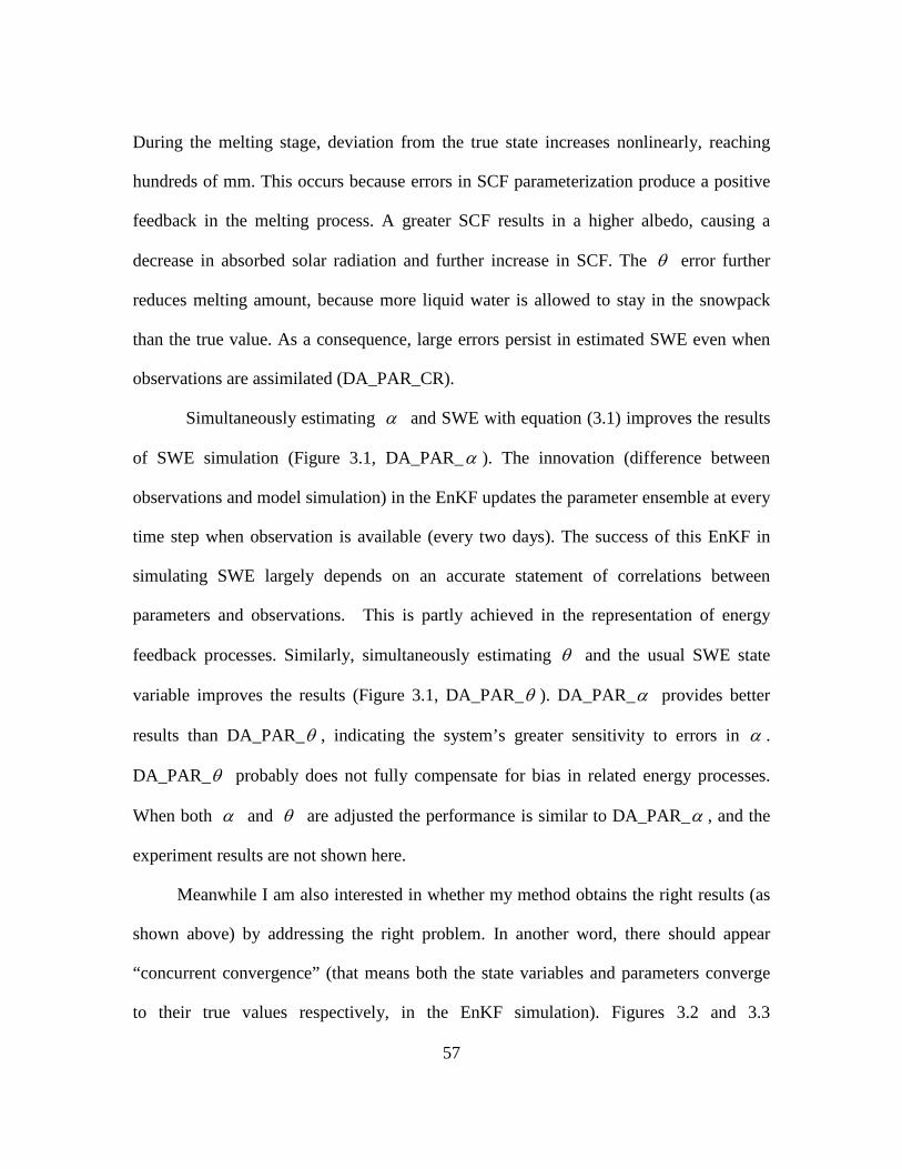
57
During the melting stage, deviation from the true state increases nonlinearly, reaching
hundreds of mm. This occurs because errors in SCF parameterization produce a positive
feedback in the melting process. A greater SCF results in a higher albedo, causing a
decrease in absorbed solar radiation and further increase in SCF. The θ error further
reduces melting amount, because more liquid water is allowed to stay in the snowpack
than the true value. As a consequence, large errors persist in estimated SWE even when
observations are assimilated (DA_PAR_CR).
Simultaneously estimating α and SWE with equation (3.1) improves the results
of SWE simulation (Figure 3.1, DA_PAR_α ). The innovation (difference between
observations and model simulation) in the EnKF updates the parameter ensemble at every
time step when observation is available (every two days). The success of this EnKF in
simulating SWE largely depends on an accurate statement of correlations between
parameters and observations. This is partly achieved in the representation of energy
feedback processes. Similarly, simultaneously estimating θ and the usual SWE state
variable improves the results (Figure 3.1, DA_PAR_θ ). DA_PAR_α provides better
results than DA_PAR_θ , indicating the system’s greater sensitivity to errors in α .
DA_PAR_θ probably does not fully compensate for bias in related energy processes.
When both α and θ are adjusted the performance is similar to DA_PAR_α , and the
experiment results are not shown here.
Meanwhile I am also interested in whether my method obtains the right results (as
shown above) by addressing the right problem. In another word, there should appear
“concurrent convergence” (that means both the state variables and parameters converge
to their true values respectively, in the EnKF simulation). Figures 3.2 and 3.3
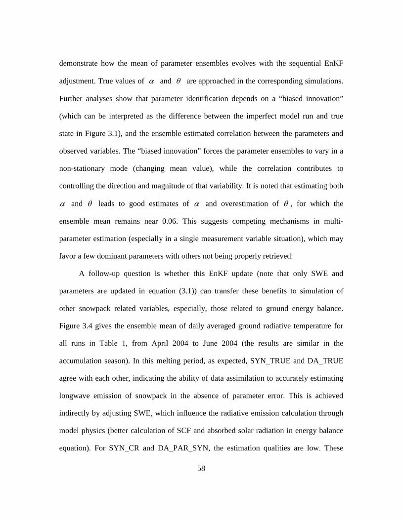
58
demonstrate how the mean of parameter ensembles evolves with the sequential EnKF
adjustment. True values of α and θ are approached in the corresponding simulations.
Further analyses show that parameter identification depends on a “biased innovation”
(which can be interpreted as the difference between the imperfect model run and true
state in Figure 3.1), and the ensemble estimated correlation between the parameters and
observed variables. The “biased innovation” forces the parameter ensembles to vary in a
non-stationary mode (changing mean value), while the correlation contributes to
controlling the direction and magnitude of that variability. It is noted that estimating both
α and θ leads to good estimates of α and overestimation of θ , for which the
ensemble mean remains near 0.06. This suggests competing mechanisms in multi-
parameter estimation (especially in a single measurement variable situation), which may
favor a few dominant parameters with others not being properly retrieved.
A follow-up question is whether this EnKF update (note that only SWE and
parameters are updated in equation (3.1)) can transfer these benefits to simulation of
other snowpack related variables, especially, those related to ground energy balance.
Figure 3.4 gives the ensemble mean of daily averaged ground radiative temperature for
all runs in Table 1, from April 2004 to June 2004 (the results are similar in the
accumulation season). In this melting period, as expected, SYN_TRUE and DA_TRUE
agree with each other, indicating the ability of data assimilation to accurately estimating
longwave emission of snowpack in the absence of parameter error. This is achieved
indirectly by adjusting SWE, which influence the radiative emission calculation through
model physics (better calculation of SCF and absorbed solar radiation in energy balance
equation). For SYN_CR and DA_PAR_SYN, the estimation qualities are low. These
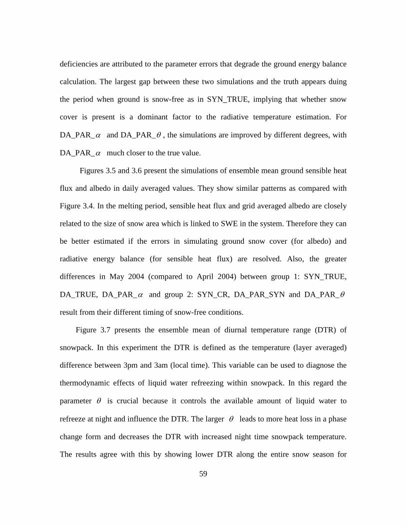
59
deficiencies are attributed to the parameter errors that degrade the ground energy balance
calculation. The largest gap between these two simulations and the truth appears duing
the period when ground is snow-free as in SYN_TRUE, implying that whether snow
cover is present is a dominant factor to the radiative temperature estimation. For
DA_PAR_α and DA_PAR_θ , the simulations are improved by different degrees, with
DA_PAR_α much closer to the true value.
Figures 3.5 and 3.6 present the simulations of ensemble mean ground sensible heat
flux and albedo in daily averaged values. They show similar patterns as compared with
Figure 3.4. In the melting period, sensible heat flux and grid averaged albedo are closely
related to the size of snow area which is linked to SWE in the system. Therefore they can
be better estimated if the errors in simulating ground snow cover (for albedo) and
radiative energy balance (for sensible heat flux) are resolved. Also, the greater
differences in May 2004 (compared to April 2004) between group 1: SYN_TRUE,
DA_TRUE, DA_PAR_α and group 2: SYN_CR, DA_PAR_SYN and DA_PAR_θ
result from their different timing of snow-free conditions.
Figure 3.7 presents the ensemble mean of diurnal temperature range (DTR) of
snowpack. In this experiment the DTR is defined as the temperature (layer averaged)
difference between 3pm and 3am (local time). This variable can be used to diagnose the
thermodynamic effects of liquid water refreezing within snowpack. In this regard the
parameter θ is crucial because it controls the available amount of liquid water to
refreeze at night and influence the DTR. The larger θ leads to more heat loss in a phase
change form and decreases the DTR with increased night time snowpack temperature.
The results agree with this by showing lower DTR along the entire snow season for
60
simulations with erroneous θ (SYN_CR, DA_PAR_SYN). DA_PAR_α also
underestimates DTR, demonstrating the independence between α adjustment and the
night time refreezing process. Estimating θ enables DA_PAR_θ to better capture the
amplitude of DTR, which much more resembles the true value than DA_PAR_α .
3.5 EFFECTS OF STRUCTURAL ERROR ON PARAMETER ESTIMATION
This section only investigates a simple case of structural error in snowpack
simulation, to facilitate a straightforward diagnose of its effects. Here a primary goal is to
keep the diagnostic framework simple and tractable, recognizing that complicated
structural error behavior may result from incorporating multiple processes and their
nonlinear interaction. Situations consisting of more complex structure errors would be
valuable topics for further research. Another SCF parameterization (replacing equation
3.3) is introduced and represents the structural error. It is shown in equation (3.6). In
addition to the above mentioned simplicity, at least two reasons are considered to
construct the error in this way. First, both two parameterizations share the common role
in the model architecture (representing grid-scale snow cover-snow depth relationship),
so they are comparable. Second, they differ greatly in their formulation, representing
significant structural difference.
Two simulations are designed. The DA_STRUCT_TRUE is the perfect-model-
structure run using equation (3.3), and starts with an erroneous θ =0.6. The
DA_STRUCT_NEW uses equation (3.6) with dZ ln as the adjustable parameter.
dZ ln characterizes the roughness length of ground and is assumed uncertain in
DA_STRUCT_NEW. To construct a comparable framework, all other structural and

61
parametric features in DA_STRUCT_TRUE and DA_STRUCT_NEW are the same as in
SYN_TRUE. Both of them assimilate a common dataset of SWE generated with the same
approach in section 3.3.
snod
sno
hZ
hSCF
+=
10 (3.6)
As mentioned in section 3.2, the selection of 0Q in equation (2) influences the
trajectory of parameter ensemble. To ensure a fair comparison, this work run the above
simulations with different 0Q , to obtain enough spread to lead to the dependable results.
In addition, the dependence of system performance and parameter retrieval on the
selection of initial value of dZ ln has been considered. My preliminary test found that
varying this input did not affect the simulation too much, so use 0dZ = 0.01 (a default
value for CLM2.0, 0dZ denotes the initial value of dZ ).
Figures 3.8 and 3.9 display the error (ensemble mean SWE minus corresponding
true value) of DA_STRUCT_TRUE and DA_STRUCT_NEW respectively, for each of
their own 0Q used to constrain the parameter ensemble variance. Note that each curve is
given in the same color as the label showing magnitude of square root of 0Q (std). Here
std is represented by a number multiplying the initial value. Tables 3.3, 3.4 give the
temporal mean of these errors (in absolute value) for DA_STRUCT_TRUE and
DA_STRUCT_NEW, respectively. Agreeing with results in section 3.3,
DA_STRUCT_TRUE performs well in estimating SWE for most of the 0Q selected,
except that the std equals half of 0α (its SWE error is still much lower than in the data
assimilation run without parameter estimation, not shown here). On the other hand,

62
DA_STRUCT_NEW performs almost equally well in estimating SWE (only with
significantly larger error for std=1/4 0dZ , while its SWE error is still much lower than the
data assimilation run without parameter estimation, not shown here). Moreover, the same
pattern exists in both figures; the error remains low at accumulation period and peaks at
melting period. The evolution of parameter ensemble stops when the ground is snow-free
for every ensemble member.
Figures 3.10 and 3.11 show how the parameters (ensemble mean) are updated in
each simulation. A difference emerges in this comparison: α converges at the end of
simulation to around 1.7 for different 0Q , while dZ ( dZ represents the ensemble
mean of dZ ) diverges to significantly different values for different 0Q . Further
inclusion of a broader range of 0Q in DA_STRUCT_NEW (including std=1/8, …to
3 0dZ , which can give a reasonable performance in SWE estimation) don’t result in an
evident convergence zone. This has been shown in Tables 3.5, 3.6, where a broad
spectrum of 0Q have been tested and the retrieved parameter have been given for
DA_STRUCT_TRUE and DA_STRUCT_NEW. These results imply that
DA_STRUCT_NEW is likely to reduce the transferability of estimated parameter
because no consensus can be made about dZ .
To test the reliability of the above results, also concerning that the most appropriate
model structure would be usually unknown for regions without adequate measurements, a
“symmetric experiment” is given, where equation (3.6) is the synthetic true
parameterization (structure) in the ensemble data assimilation framework, and equation

63
(3.3) represents the structural error. In this experiment, the observation is derived from
the synthetic true simulation with (3.6) (true dZ =0.01), and assimilated into two
different data assimilation run with equation (3.6) (DA_STRUCT_TRUE_2) and (3.3)
(DA_STRUCT_NEW _2), respectively. In general, results in this experiment are very
similar to those shown above. That means the state variable can be well estimated in both
DA_STRUCT_TRUE_2 and DA_STRUCT_NEW _2, while the parameters converge in
DA_STRUCT_TRUE_2 ( dZ ), and don’t show an evident convergence in
DA_STRUCT_NEW _2 (α ). The details of these results are omitted here.
3.6 DISCUSSION
3.6.1 Parameter estimation convergence/divergence
In a perfect-model-structure run, parameter estimation in the ensemble snow data
assimilation has shown promise in accurately estimating a suite of land surface variables.
In this scenario, both variables and parameters converge to the true value simultaneously,
which is in contrast to the result in the imperfect-model-structure run.
A hypothetical explanation for the above result is that, driven by model structural
error, each 0Q , a degree of freedom constraining the parameter variance, seems to
become an independent condition and leads the stochastic update to a unique value in the
parameter space, while to the structure-error free case (DA_STRUCT_TRUE), the effects
of 0Q on parameter retrieval appear to be refrained, with different 0Q amounting to
largely equivalent constraints, which leads to parameter convergence.
64
The insensitivity of parameter estimation to the magnitude of prescribed parameter
error 0Q in the perfect-model-structure run (in which the forcing and observation error
are also perfectly represented) is somehow analogous to results shown in Crow and Van
Loon (2006), which demonstrated that, if the single error (only refer to random error, the
model structure is perfect) source and observation error are both perfectly represented in
the EnKF soil moisture data assimilation system, the overestimation of model error has
little impact on the accuracy of retrieved state variable. This linkage implies that the
results of parameter convergence (or not) shown here can be interpreted from the
observational control perspective, where the structural accuracy might foster a robust
relation between observation (invariant for different 0Q ) and the parameter update. This
relationship is important to the availability of a relatively consistent trajectory for the
sequential parameter search against the variation of 0Q . In this experiment, this
connection can be partly reflected by the refrained updates of α (in the ablation stage)
where 0Q have been increased (Figure 10, also Table 5, same observation data are used
in different simulations). On the other side, the structural error may distort the
representation of parameter uncertainty through ensemble and attenuate this connection
between observation (structural invariant) and parameter (in the problematic structure),
therefore hinder the presence of a consistent parameter evolution among different 0Q .
This deficiency can be well characterized by an excessively broad divergence zone in the
corresponding 0Q space (Figure 3.11 and Table 3.6, same observation data are used in
different simulations).

65
The detailed features associated with the 0Q space may be dependent on a number
of complex issues such as the structural role in parameter estimation, which is modulated
by the EnKF effects associated with ensemble space dynamics (e.g., using ensemble
covariance to calculate increments), as well as the observation control on parameter
evolution. Evaluation of the above potential explanations warrants further investigation,
which may include how to measure these connections and mechanisms (e.g. between the
degree of freedom 0Q and parameter evolution), whether they are ad-hoc, and what they
are conditioned on.
In addition, the above parameter search divergence in DA_STRUCT_NEW could
be alleviated by developing a more physically based method to estimate 0Q or predict
the variance of parameter ensemble, for example, linking them to the flow-dependent
error covariance of state variables (an approach similar to bias estimation in De Lannoy
et al., 2008). When 0Q or parameter variance could be calculated through a physically
robust scheme, this divergence problem becomes trivial, and the optimal parameter can
be identified. However, a fully dynamical parameterization of these ensemble-space
parameters can be difficult, considering the nature of parameter (a physically constant
value) in the snow hydrological system.
3.6.2 Several limitations in current research
This study may have limitations in several aspects. First, there are alternative
approaches to achieve the simultaneous state and parameter estimation that do not require
time varying parameter (ensemble) (e.g., Vrugt et al., 2005, Clark and Vrugt, 2006). The
relative strengths and limitations among these algorithms are still not clear, and their
66
optimal design and application remain an active research area in the land surface system
characterization (Moradkhani et al., 2005).
It is also recognized that the structural error and associated parameter adopted in
my research are simplistic, because it only involves a specific parameterization equation.
In this regard an extended study of temporal behavior of parameter statistics (e.g.,
ensemble mean) with elaborately perturbed structures in the EnKF simulation is
suggested. Along this line I highlight the importance of testing large number of
parameters embedded in multiple model structural components. Niu and Yang (2004)
discussed several important physical processes governing snowpack evolution and their
various representation in LSM, for example, canopy interception (with or without),
radiation transfer (traditional scheme or revised two-stream), and below canopy
turbulence. The uncertainties in simulating these processes can be incorporated into
current framework as structural error. The interactions among these structural
components may give rise to far more complicated results (e.g., different relations
between 0Q and parameter search convergence) than those revealed in this work. In
addition, because parameters in LSM can have significant and complex interactions (e.g.,
Rosero et al., 2009), it is worthy to investigate the appropriate size of parameters
involved in this estimation framework, for example, whether to use all snowpack related
parameters or to select part of them.
3.7 CONCLUDING REMARKS
This study investigates the performance of parameter estimation in snow data
assimilation experiments, and its dependency on the model structure. In the synthetic
67
EnKF simulation without model structure error, simultaneous state and parameter
estimation is effective. The algorithm reduces the systematic error in SWE estimates and
accurately retrieves the parameter values. Further, a suite of other land surface variables,
especially those related to snowpack (and ground) energy balance, are better estimated
when the parameters are correctly updated. Another important implication from this
research is that, in the presence of model structural error, parameter search convergence
and accurate estimation of state variables might not be simultaneously achieved,
indicating the potential problem resulting from structure error. In particular, this work
introduces a new degree of freedom, parameter variance constraint, in the parameter
estimation framework, and find that imperfect-model-structure leads to parameter
divergence over a broad zone in this constraint space. This is in contrast to the clearly
retrieved parameter convergence in the perfect-model-structure run. These results
demonstrate that with a problematic model structure, good performance in estimating
state variables does not necessarily mean that the associated parameter estimation is
reliable. In this sense, my investigation may provide a way for diagnosing structural
robustness in the ensemble snow data assimilation system. It is also emphasized that the
generality of this result should be investigated with a more complex structural error
configuration (e.g., a combination of multiple structural components).

68
Table 3.1. Description of simulations in experiments.
SYN_CR Synthetic ensemble simulation with parameters error but without synthetic data assimilation
DA_PAR_CR Synthetic ensemble simulation with parameters error and synthetic data assimilation
DA_PAR_α Synthetic ensemble simulation with parameters error, synthetic data assimilation and parameter estimation of α
DA_PAR_θ Synthetic ensemble simulation with parameters error, synthetic data assimilation and parameter estimation of θ
DA_TRUE Synthetic ensemble simulation with true parameters and synthetic data assimilation
SYN_TRUE Synthetic truth from a particular forcing set and true parameters
DA_STRUCT_TRUE Synthetic ensemble simulation with parameter error in α , other feature same to DA_TRUE
DA_STRUCT_NEW Synthetic ensemble simulation with parameter error in dZ , also with equation (3.6),
other feature same to DA_TRUE
DA_STRUCT_TRUE_2 Synthetic ensemble simulation with parameter error in dZ , assimilates observation
from another synthetic true with equation (3.6), other feature same to DA_TRUE DA_STRUCT_NEW_2 Synthetic ensemble simulation with parameter error in α , assimilates observation
from another synthetic true with equation (3.6), other feature same to DA_TRUE.

69
Table 3.2. The Nash-Sutcliffe efficiency for ensemble mean of different simulation shown in Figure 3.1. The value equal to 1 represents the perfect simulation, with the value the larger the better.
DA_TRUE DA_PAR_α DA_PAR_θ DA_PAR_CR SYN_CR 0.98 0.96 0.61 0.22 -1.21

70
Table 3.3. The temporal averaged error in SWE (ensemble mean minus the true value) for parameter estimation run DA_STRUCT_TRUE with different 0Q
shown in Figure 3.8. Here 0Q is represented by standard deviation (0Q ),
which is equal to R multiplying the initial parameter: Std=R* 0α .
R 1/4 1/2 3/4 1 3/2
Error (mm) 7.49 11.36 8.08 7.68 7.71

71
Table 3.4. The temporal averaged error in SWE (ensemble mean minus the true value) for parameter estimation run DA_STRUCT_NEW with different 0Q
shown in Figure 3.9. Here 0Q is represented by standard deviation (0Q ),
which is equal to R multiplying the initial parameter: Std=R* 0α .
R 1/4 1/2 3/4 1 3/2
Error (mm) 19.96 8.86 8.61 8.63 8.62

72
Table 3.5. The ensemble mean of α retrieved in DA_STRUCT_TRUE when ground is snow-free in May (for every ensemble member), as a function of different
0Q constraining the parameter variance. Here 0Q is represented by
standard deviation ( 0Q ), which is equal to R multiplying the initial
parameter: Std=R*0α .
R 1/8 1/4 1/2 3/4 1 11/4 3/2 2 5/2 3
α 1.70 1.72 1.73 1.77 1.78 1.79 1.81 1.83 1.89 1.96
152.0=−
Min
MinMax
α
αα

73
Table 3.6. The dZ retrieved in DA_STRUCT_NEW when ground is snow-free in May
(for every ensemble member), as a function of different 0Q constraining
the parameter variance. Here 0Q is represented by standard deviation
( 0Q ), which is equal to R multiplying the initial parameter: Std=R* 0dZ .
R 1/8 1/4 1/2 3/4 1 11/4 3/2 2 5/2 3
dZ 0.0026 0.0042 0.0070 0.0090 0.0108 0.0129 0.0142 0.0181 0.0266 0.0362
9.12=−
Mind
MindMaxd
Z
ZZ
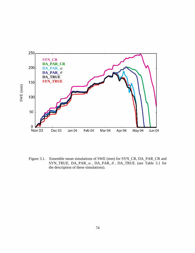
74
Figure 3.1. Ensemble mean simulations of SWE (mm) for SYN_CR, DA_PAR_CR and SYN_TRUE, DA_PAR_α , DA_PAR_θ , DA_TRUE. (see Table 3.1 for the description of these simulations).
SW
E (
mm
)
SYN_CR DA_PAR_CR DA_PAR_α DA_PAR_θ DA_TRUE SYN_TRUE
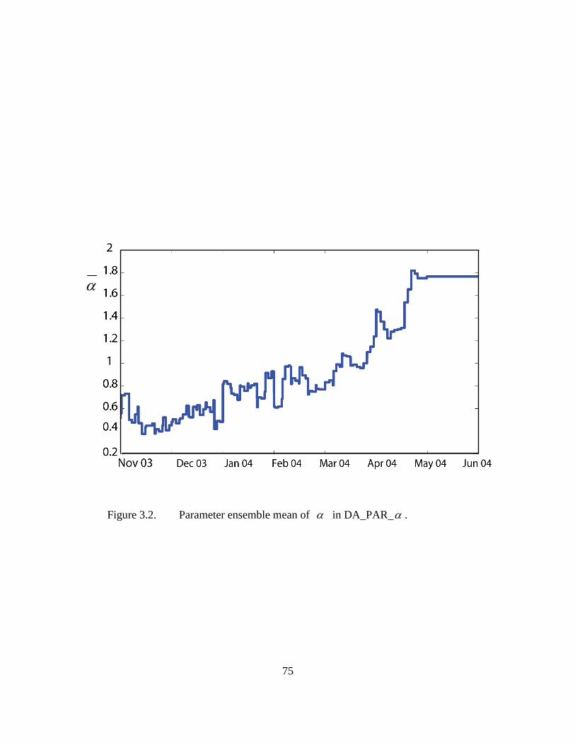
75
α
Figure 3.2. Parameter ensemble mean of α in DA_PAR_α .
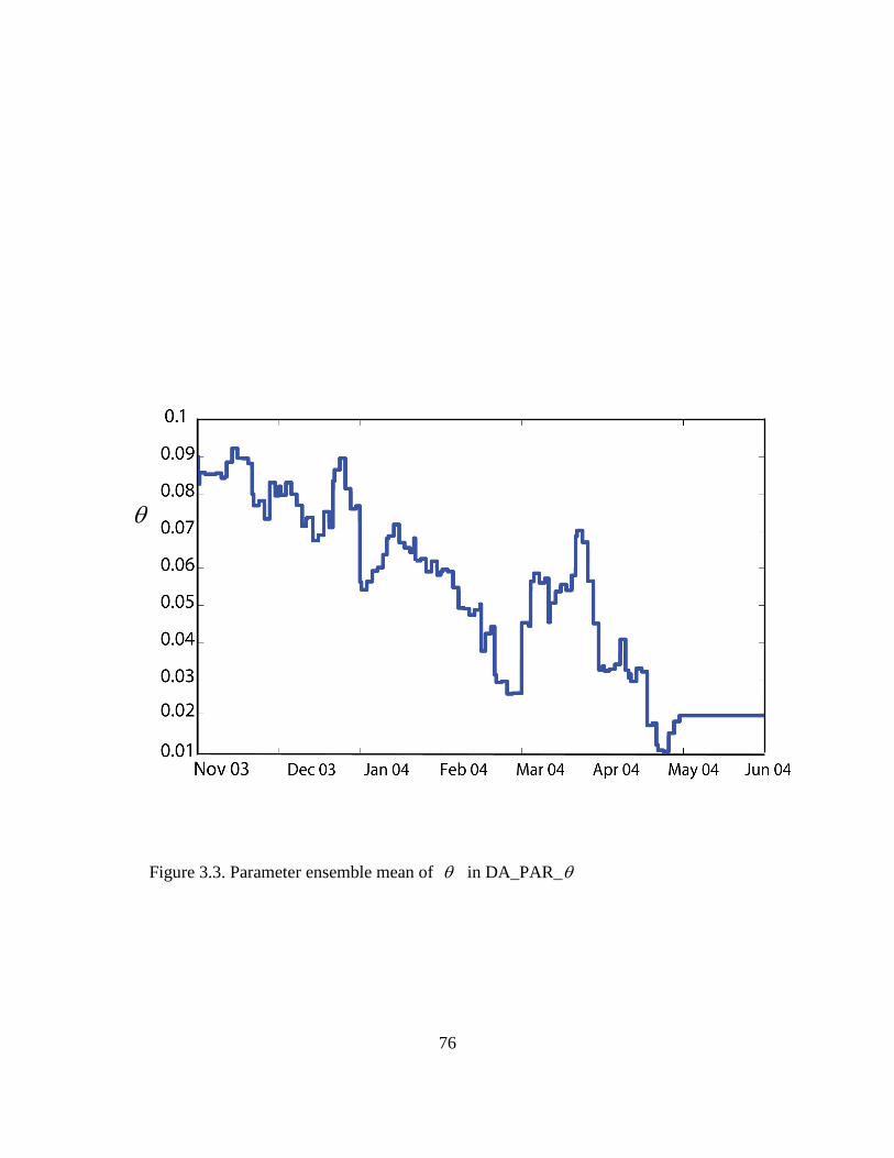
76
θ
Figure 3.3. Parameter ensemble mean of θ in DA_PAR_θ

77
`
Figure 3.4. Ensemble mean of DTR (diurnal temperature range) for SYN_CR, DA_PAR_CR and SYN_TRUE, DA_PAR_α , DA_PAR_θ , DA_TRUE.
DT
R (◦
C)
SYN_CR DA_PAR_CR DA_PAR_α DA_PAR_θ DA_TRUE SYN_TRUE
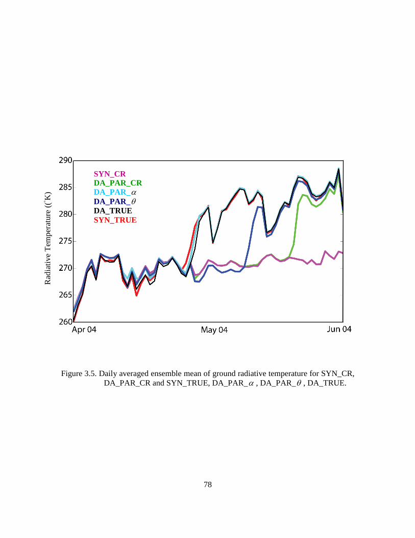
78
Figure 3.5. Daily averaged ensemble mean of ground radiative temperature for SYN_CR, DA_PAR_CR and SYN_TRUE, DA_PAR_α , DA_PAR_θ , DA_TRUE.
SYN_CR DA_PAR_CR DA_PAR_α DA_PAR_θ DA_TRUE SYN_TRUE
Rad
iativ
e T
empe
ratu
re (
(◦K
)

79
Figure 3.6. Daily averaged ensemble mean sensible heat flux for SYN_CR, DA_PAR_CR and SYN_TRUE, DA_PAR_α , DA_PAR_θ , DA_TRUE.
SYN_CR DA_PAR_CR DA_PAR_α DA_PAR_θ DA_TRUE SYN_TRUE
Sen
sibl
e H
eat F
lux
(W/m2 )
SYN_CR DA_PAR_CR DA_PAR_α DA_PAR_θ DA_TRUE SYN_TRUE

80
a
Figure 3.7. Daily averaged ensemble mean albedo for SYN_CR, DA_PAR_CR and SYN_TRUE, DA_PAR_α , DA_PAR_θ , DA_TRUE.
SYN_CR DA_PAR_CR DA_PAR_α DA_PAR_θ DA_TRUE SYN_TRUE
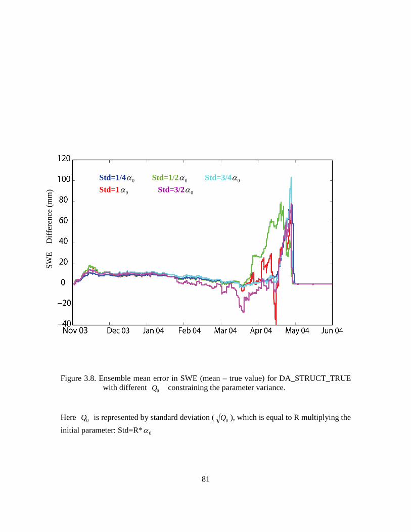
81
Figure 3.8. Ensemble mean error in SWE (mean – true value) for DA_STRUCT_TRUE with different 0Q constraining the parameter variance.
Here 0Q is represented by standard deviation (0Q ), which is equal to R multiplying the
initial parameter: Std=R* 0α
Std=1/4 0α Std=1/2 0α Std=3/4 0α
Std=1 0α Std=3/2 0α
SW
E
Diff
eren
ce (
mm
)
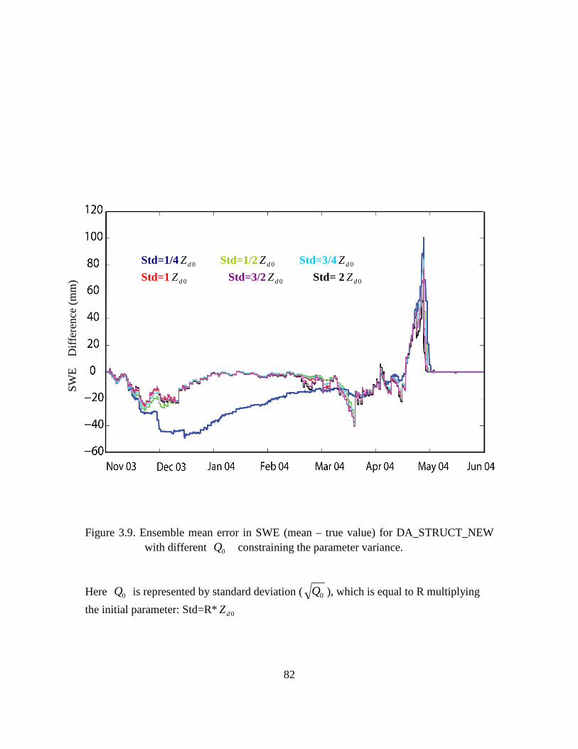
82
Figure 3.9. Ensemble mean error in SWE (mean – true value) for DA_STRUCT_NEW with different 0Q constraining the parameter variance.
Here 0Q is represented by standard deviation (0Q ), which is equal to R multiplying
the initial parameter: Std=R* 0dZ
Std=1/4 0dZ Std=1/2 0dZ Std=3/4 0dZ
Std=1 0dZ Std=3/2 0dZ Std= 2 0dZ
SW
E
Diff
eren
ce (
mm
)
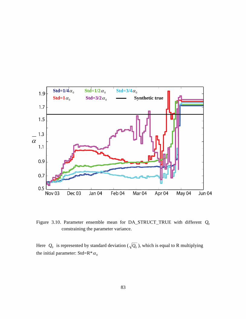
83
Figure 3.10. Parameter ensemble mean for DA_STRUCT_TRUE with different 0Q constraining the parameter variance.
Here 0Q is represented by standard deviation (0Q ), which is equal to R multiplying
the initial parameter: Std=R*0α
Std=1/4 0α Std=1/2 0α Std=3/4 0α
Std=1 0α Std=3/2 0α Synthetic true
α

84
Figure 3.11. Parameter ensemble mean for DA_STRUCT_NEW with different 0Q constraining the parameter variance.
Here 0Q is represented by standard deviation (0Q ), which is equal to R multiplying
the initial parameter: Std=R* 0dZ
dZ
Std=1/4 0dZ Std=1/2 0dZ
Std=3/4 0dZ Std=1 0dZ
Std=3/2 0dZ Std= 2 0dZ

85
Chapter 4: Multi-sensor snow data assimilation at continental-scale: the value of GRACE TWS information
4.1 ABSTRACT
This investigation establishes a multi-sensor snow data assimilation system (for data
over North America from Jan 2002 to Jun 2007) with improved estimation of snowpack
(in particular, SWE and snow depth) by incorporating both GRACE TWS and MODIS
SCF information into the CLM. The different properties associated with the TWS and
SCF observations have been accommodated through a unified approach using the
ensemble Kalman filter (EnKF) and smoother (EnKS). Results show that this multi-
sensor approach can provide significant improvements over the traditional MODIS only
approach, for example, in Saint Lawrence, Fraser, Mackenzie, Churchill & Nelson, and
Yukon river basins, and the south-west rim of Hudson Bay. In mid-latitudes, for example,
the North Central and Missouri river basins, inclusion of GRACE information preserves
the advantages (compared with Open Loop) shown in the MODIS only run. However, in
some high latitude areas and given months, the open loop run can have a comparable or
even better performance, implying considerable room for refinements of the multi-sensor
algorithm. In addition, ensemble based metrics are calculated and interpreted at domain
wide. They indicate the potential importance of accurate representation of SWE auto-
covariance in assimilating TWS observations, and the regional and/or seasonal
dependence of the GRACE capability in reducing ensemble variance. These analyses
contribute to clarifying the effects of GRACE’s special features (e.g., a vertical integral

86
of different land water storage changes, coarse spatial and temporal resolution) in the
snow data assimilation system.
4.2 INTRODUCTION
Snow is an important component of the earth climate system. At continental and inter-
annual scales SCF and SWE have large variations, depending on atmospheric circulation
patterns. High albedo and low thermal conductivity of snow significantly affect land
surface energy and water budgets. Consequently, accurate estimation of snowpack
properties at large scale is important for various research areas, for example: (1)
hydrological prediction and water resources management, especially for those regions in
which fresh water availability is heavily dependent on snow melt (Barnett et al., 2005);
(2) evaluation of coupled General Circulation Models (GCMs) in terms of their ability to
represent observed snow dynamics (Frei and Gong, 2005); (3) climate trend
quantification in cold regions; and (4) land-atmosphere-ocean interactions associated
with snow cover (Gong et al., 2003).
In recent years, derivation of high quality snow datasets, SWE in particular, has
increasingly relied on data assimilation technology, which optimally blends numerical
model results and remotely sensed information to generate more accurate and physically
consistent products. Compared with ground observations that are scattered and often do
not represent regional averages, satellite observations effectively expand the spatial
coverage to regional and continental scales. Among satellites observations, SCF products
are unique in their estimation of SWE distribution when compared with other products,
such as microwave-based estimates. Snow has distinct reflectance effects in visible and
87
infrared bands (Hall et al., 2002), which can be measured at relatively high spatial
resolution (Hall et al., 2002; Hall and Riggs, 2007). Further, the SCF retrieval with these
algorithms does not require information about the micro-scale internal properties of
snowpack, for example, density, grain size, and liquid water content, although implicit
relations may be involved. Consequently, remotely sensed SCF information has been
increasingly used to correct SWE estimates from land surface models (LSMs), via the
EnKF technology (e.g., Andreadis and Lettenmaier, 2006; Clark et al., 2006; Su et al.,
2008). However, a number of limitations degrade the quality of assimilated SWE
products, or hamper application in specific climatic and geographic environments,
including:
(1) Low correlation between SCF and SWE when model grid averaged SWE
exceeds a threshold. In this situation, small changes in SCF lead to a wide range of SWE
for a given location. Several studies (Clark et al., 2006; Su et al., 2008) found the SCF
assimilation performs best with partial snow cover (e.g., ephemeral snow in mountains
and grasslands), but performs poorly when the SCF signal is saturated (near 100% SCF)
and insensitive to further SWE increments (e.g., during the accumulation season over
boreal forest and tundra).
(2) Parameter errors in the observational operator. A key component of the SCF
approach is a parameterized relationship (observation operator or function) between SCF
and SWE at each model grid. Various observation functions have been utilized in the
literature (Andreadis and Lettenmaier, 2006; Clark et al., 2006; Su et al., 2008), each
having some key parameters characterizing geographic and scale effects. These

88
distributed parameters are usually difficult to measure (because they rely on intensive
calibration) and their errors can degrade SWE retrievals.
(3) Errors in satellite-derived SCF data. Although the EnKF algorithm can account
for observational noise, SCF error magnitude (variance) can be difficult to quantify in
certain environments like mountains (Hall and Riggs, 2007), or when obscured by cloud
cover and vegetation (Hall and Riggs, 2007). These environments can also lead to
systematic errors not accommodated by current data assimilation systems.
These three types of errors tend to be magnified when present simultaneously. For
example, if the SCF signal is saturated during a boreal forest winter, a small amount of
bias in SCF data or uncertainty in parameters may lead to significant errors in the
observation operator and hence SWE update.
All these limitations motivate me to develop a new methodology for improving
continental scale SWE and relevant estimates, using additional information from other
satellites. Because SCF observations mainly characterize the spatial distribution of
snowpack, inclusion of further model constraints such as mass and energy terms should
be complementary. An analogous approach has been applied in estimating soil moisture,
evapotranspiration, and other hydrological states and fluxes (Renzullo et al., 2008),
where multiple data resources are shown to improve estimates. Nevertheless, there has
been little research devoted to exploring the nature of multi-sensor or multi-frequency
(for radiometer) snow data assimilation. Among the first studies are those of Durand and
Margulis (2006, 2007), but their synthetic experiments are confined to point and river
basin scale snowpack, and focus on radiometric observations.

89
Monthly global TWS estimates have been available from the GRACE satellite
system since 2002. GRACE provides estimates of total surface mass change from month
to month using changes in Earth's gravity field, with a spatial resolution comparable to
satellite altitude of about 400 km. Thus, unlike visible band instruments, GRACE can
monitor ground under all-weather conditions (as do microwave radiometers) and
measures integrated total land water storage changes from canopy to deep groundwater.
Much research has focused on extracting from GRACE meaningful trends and
variabilities of individual TWS components (e.g., soil moisture, snow, groundwater)
(Syde et al., 2008; Rodell et al., 2004; Niu et al., 2007). More recently Zaitchik et al
(2008) incorporated GRACE TWS data into a land surface model using an ensemble
Kalman smoother (EnKS) to improve water storage and flux estimates in the Mississippi
River basin (where snowpack was simply updated without direct calculation of SWE
increments from its ensemble statistics).
In this study I use GRACE TWS measurements to complement MODIS SCF data
assimilation over North America. Integration of radiometer (at visible and infrared bands)
and gravity measurements into a land surface model over such a large domain has
received little attention. Accordingly I focus on the following questions: How can the two
types of snow information that have distinct physical and geographic features be jointly
assimilated? Can GRACE data assimilation improve SWE and snow depth retrival,
relative to MODIS only data assimilation? How do these improvements (multi-sensor vs.
single sensor), if any, vary geographically and with what underlying mechanisms?
Specific attention is given to the special properties of GRACE TWS data (its spatial and
temporal resolution). Some controlling factor for GRACE TWS assimilation and its

90
capability of reducing errors were interpreted quantitatively. The central purpose was to
develop observational and algorithmic techniques for accurately characterizing SWE and
other cold region hydrological variables.
Section 4.3 introduces data and methods applied in the data assimilation
experiments. Section 4.4 describes in detail how these experiments were implemented.
The results are analyzed in section 4.5 and section 4.6 provides interpretations and
comments on specific features of the multi-sensor data assimilation. Concluding remarks
are given in section 4.7.
4.3 DATA AND METHODOLOGY
4.3.1. MODIS and GRACE satellite datasets
Daily MODIS SCF data at 0.05º resolution (MOD10C1) are used in this study.
MODIS uses 7 spectral bands to retrieve land surface properties. Its snow mapping
algorithm estimates SCF using Normalized Difference of Snow Index (NDSI) (Hall et al.,
2002), and is able to distinguish between snow and clouds (Hall et al., 2002). Su et al.
(2008) described the MODIS data processing used in this study, including spatial
upscaling of raw data and cloud parameter selection for quality control.
GRACE monthly gravity fields are represented as spherical harmonics to degree
and order 60, with most time variable atmospheric and oceanic gravitational effects
removed during data processing. Remaining gravity changes are interpreted as monthly
changes in vertically integrated water storage components, for example, snow, soil
moisture, and groundwater. GRACE estimates are smoothed with a Gaussian averaging
kernel with a 500 km radius, and filtered to remove longitudinal stripes that are a

91
recognized noise component in current solutions (Chen et al., 2008). GRACE estimates
are then represented on 4 º by 4 º tiles using bilinear interpolation for compatibility with
the model grid configuration (1 º by 1 º over North America). These time series span the
period from November 2002 to May 2007, with missing values in December 2002 and
June 2003. Here the TWS data are in their multi-year anomaly form, in which the long
term mean of TWS is subtracted from each monthly value. In practice, GRACE time
series values are computed from observations taken from about one-half month before to
one-half month after the date assigned to the sample.
According to their physical features, MODIS and GRACE contain different
information relevant to SWE retrieval. MODIS measures SCF at high spatial resolution
compared to both GRACE and the numerical model, observing both accumulation and
ablation with approximately the same level of accuracy. GRACE measures total column
water storage change at a far coarser spatial and temporal scale, and does not contain
information about the individual components contributing to water storage changes.
However, SWE is expected to be the dominant variable component of TWS in winter in
cold regions (Niu et al., 2007). Its relative contribution diminishes during melting, when
MODIS is thought to be more closely correlated to SWE. GRACE estimates are not
affected by vegetation (except as its mass changes), topography and cloud cover, and is
useful in conditions when the value of MODIS is limited by these influences.
4.3.2 Observation based climatologic SWE and snow depth datasets
The Canadian Meteorological Center (CMC) snow depth and SWE climatology data
(1969-1997) (Brown et al., 2003) were used for validation purpose. These provide daily
92
snow depth and SWE at 0.25 º resolution. The snow estimates were obtained by
combining abundant station observations in U.S. and Canada with model simulations by
an optimum interpolation scheme (Brown et al., 2003). These observationally based
datasets are regarded as the best available reference for this research.
4.3.3 Land surface model
The CLM used in these experiments includes an enhanced frozen soil hydrology
scheme and a new aquifer dynamical scheme, among other modifications (Niu and Yang,
2006; Niu et al., 2007). The aquifer model, by explicitly simulating ground water
dynamics, facilitates assimilating TWS observations. Water storage in the saturated zone
is a prognostic variable and directly represented in the calculation of TWS in each grid,
facilitating combination of GRACE data with model estimates (Zaitchik et al., 2008). In
addition, CLM’s sophisticated representation of frozen soil hydrology has improved its
ability to characterize soil moisture and runoff variability in cold regions, thus reducing
the systematic error in TWS estimation. These enhancements reduce model biases (see
Niu and Yang, 2006; Niu et al., 2007 for more discussion). The negative effects of model
biases cannot be eliminated by updating state variables alone, and model bias can result
in complex effects into the data assimilation system (e.g., c.f. De Lannoy et al. , 2008).
4.3.4 The ensemble Kalman filter and smoother
The EnKF (Evensen, 1994, 2003) and EnKS are used to incorporate MODIS and
GRACE data into CLM, respectively. The choice of algorithms (the EnKF for MODIS
SCF assimilation and EnKS for GRACE TWS assimilation) depends on the nature of
satellite datasets.

93
The EnKF treats some crucial model inputs, such as forcing data, model parameters,
and model initial conditions, as random variables, and ensembles of these inputs are
generated to represent their distributions. Each ensemble member is propagated forward
using the model until a measurement becomes available. The measurement is assimilated
into the model simulation by using the ensemble of state variables to represent a low-rank
approximation of the joint pdf between state variables and measurements. The EnKF
update is optimal only when certain assumptions are met: (1) unbiased measurements and
background (model simulated) variables; (2) Gaussian type random inputs (e.g., the
forcing errors); and (3) linear relationships between states and measurements. Given the
above properties, the EnKF is able to characterize highly nonlinear land hydrological
processes and their associated uncertainties. Such sequential data assimilation accounts
for the temporal sampling discrepancy between CLM (3-hours) and MODIS data (daily),
as discussed in Su et al. (2008) where additional details are provided.
The EnKS (Dunne et al., 2005, 2006) is theoretically similar to the EnKF but
allows for observations that: (1) are defined at different times than the model state; and
(2) span multiple periods of time comprising, for example, both current and historical
model states. Because GRACE data are at monthly intervals and CLM runs at three
hours, the EnKS is used to compare model estimates of TWS with those of GRACE and
derive updates for state variables. The update of the EnKS is:
)v)(H(K iT1
bti,T1T1t,T1
bti,
ati, +−+= XYXX (4.1)
where ati,X represents the updated ith ensemble member of the state vector, b
ti,X
represents the corresponding ensemble member simulated by the model. The ensemble
94
state vector is defined at timet , which can be a daily average value and differs from the
GRACE observation T1Y (monthly TWS anomaly with respect to a multi-year mean)
defined for a month T1. )(XH bti,T1 is the observation function for the month T1, as
obtained by integration of model TWS components over all grids within the GRACE tile
(4 º by 4 º in this study), and over all days within the month T1. The noise term iTv 1 is
randomly drawn from a Gaussian distribution (with zero mean and the variance equal to
that of the observation error) to ensure an adequate spread of the analysis ensemble
members (Burgers et al., 1998). The Kalman gain T1t,K is obtained with the same
ensemble approach as used in the EnKF,
1T11T1
btT1
bT1t, ]R))(),())[Cov(H(H,(K −+=
btT
btt XHXXXCov (4.2)
where T1R is the auto-covariance of observation error. The auto-covariance of model
simulated observation ( ))(),(Cov(H 1T1b
tTb
t XHX ), and cross covariance
( ))(H,( btT1
b XXCov t ), are estimated from inner products of corresponding ensemble
( bti,X and )(H b
ti,T1 X ) anomalies (which are ensemble minus their mean).
The EnKS provides a reasonable way to match GRACE estimates of changes in
TWS to each model simulated day. In reality GRACE estimates incorporate varied
information about any particular geographical location because orbits do not repeat. Thus
it is difficult to set a uniform frequency and associated time accurately characterizing the
satellite track at each grid. The approach appears justifiable because with slow temporal
variation at large spatial scales, the monthly samples should adequately describe TWS.

95
4.4 IMPLEMENTATION OF THE DATA ASSIMILATION EXPERIMENTS
Three experiments were designed to address questions stated in section 4.2. One is
the open loop (OL) simulation where CLM alone is used to estimate SWE and other land
variables. Second is a MODIS only (MOD) data assimilation experiment similar to that
used in Su et al. (2008). Third is the joint MODIS_GRACE (MOD_GR) data assimilation
experiment.
All simulations are driven by the meteorological forcing dataset from the Global
Land Data Assimilation System (GLDAS) at 1º×1º resolution. The GLDAS forcing data
are observationally derived fields including precipitation, air temperature, air pressure,
specific humidity, and shortwave and longwave radiation. The forcing data (e.g.,
precipitation) biases are not explicitly accounted for in this data assimilation approach,
because of the lack of such information. CLM wad run with data from Jan, 2002 to June,
2007. The ensemble runs do not assimilate observations until Nov, 2002. In MOD_GR,
the relative error in log-normal perturbation of precipitation is 65%, and the e-folding
scale of horizontal error correlations is 3 º (in both latitude and longitude) for
precipitation and temperature. A temporal correlation of 3 days is assumed for the forcing
perturbation. The selection of these forcing parameters is based on previous research on
GRACE data assimilation (Andreadis and Lettenmaier, 2006; Zaitchik et al, 2008). These
parameters are also applied in MOD. Additional experiments show that the change of
forcing error parameters in Su et al. (2008) to the above values did not influence the
MOD run significantly, and the main purpose here is to keep them the same in both MOD
and MOD_GR. All other ensemble parameters in MOD and MOD_GR are the same as in
Su et al. (2008). It is recognized that a more comprehensive description of forcing error
96
(e.g., only errors in precipitation and temperature are considered in this research) needs to
be included in further research. The ensemble size is 25, which has been demonstrated to
be suitable for large scale snow data assimilation in Su et al. (2008). Here only describes
implementation of MOD_GR with EnKS.
At each day in a given month, the MODIS SCF is integrated into the ensemble
simulation at every 1º×1º model grid as performed in the MOD experiment. Here a “fixed
interval state inflation” is applied, which periodically augments the ensemble spread of
SWE at all tiles in every CLM grid. Specifically, the SWE simulation takes the form of
tttSWEtSWE pxfx ω+= − ),( 1,, (t = every q days) (4.3)
every q days. Here f represents CLM, tω represents the perturbation on the state
variable tSWEx , with variance of Q , tp represents the perturbed forcing. At other steps
the SWE is simulated by the functionf without any state inflation:
),( 1,, ttSWEtSWE pxfx −= (t = other time steps) (4.4)
(note that if after inflation, SWE is below or equal to zero, then the inflation is not given).
This inflation scheme is tailored to the needs of ensemble simulation of SWE. The
absence of inflation may lead to too small a spread of the ensemble, degrading EnKF and
EnKS performance. On the other hand, too frequent an inflation can cause excessive
ensemble spread and unrealistic updates. Augmenting the state at each time step is not
necessary because the main source of SWE uncertainties, the forcing uncertainty, has
been dealt with elsewhere. For this reason, the selection of q and Q is largely
application specific, and here q = 6 and Q = 36 mm2 (which are representative in both
MOD and MOD_GR, as demonstrated below) are taken as domain-wide values for both

97
MOD and MOD_GR. This study does not address development of more objective ways
to select these parameters, such as the adaptive filter algorithm (Reichle et al., 2008). My
initial tests found that for MOD run, state inflation using parameters (1q and 1Q ) within
a reasonable range ( 3q1 ≥ and 21 mm06Q ≤ , which includes the case of no inflation)
affected (relative to the observational data of CMC) the data assimilation results slightly;
for MOD_GR run, a similar range ( 8q3 2 ≤≤ and 22
2 mm100Q20mm ≤≤ ) exists in
which the changes in 2q and 2Q also affected little (relative to observation data CMC)
the data assimilation results. Parameters that are significantly outside the above ranges
would dramatically alter the results in two experiments by degrading the quality of the
SWE estimates when compared with the observational dataset of CMC (detailed results
are not shown here).
At the end of the month when all the MODIS data have been assimilated, GRACE
TWS information (on 4 º by 4 º tiles) is optimally distributed into the archived daily state
vector (on 1º×1º grids) consisting of the daily averaged SWE, snow depth, canopy snow,
soil moisture, and aquifer storage. This spatial and temporal disaggregation is
accomplished by using the EnKS (equation 1) with GRACE observation error T1R set
to 20 mm, consistent with previous studies (e.g., Zaitchik et al, 2008). Because the
observation T1Y in equation (4.1) is an anomaly value (with respect to a mean over the
GRACE observation period), )(XH bti,T1 takes into account model TWS climatology at
each GRACE tile. The state vector at the last step of each month is updated with equation
(4.1), then propagated by the model to next month to repeat the above data assimilation
cycle.
98
The above method utilizes each daily ensemble of state variables ( bti,X in equation
(4.1)) to calculate the corresponding Kalman gain to give a theoretically robust estimate
of data assimilation increments, although these updates are not involved in the model
propagation. The memory of state variables update is represented by reinitializing the
simulation (with the updated state vector) at the last step of each month. My adaptation of
the EnKS could be improved, given the complexity resulting from the temporal scale
difference between GRACE data and model.
4.5 RESULTS
This work focuses on evaluating the estimates of SWE and other snow variables,
even though other updated land surface states and fluxes are also provided by the
MOD_GR simulation. An extensive assessment of the improvement in all the other
hydrological variables from the multi-sensor snow data assimilation should be addressed
in future research (initial analyses find that the impacts of MOD and MOD_GR on
estimation of water and energy fluxes (e.g., latent and sensible heat, runoff etc.), are
small at monthly scale).
4.5.1 Monthly SWE difference between MOD and MOD_GR
The spatial distribution of SWE differences between single-sensor (MOD) and
multi-sensor (MOD_GR) experiments illustrates the incremental value of GRACE
information. Figure 4.1 shows that this monthly averaged field has considerable spatial
heterogeneity in the cold season (Jan-Apr). Large changes in the SWE estimate of the
MOD_GR run (compared to MOD) are concentrated in high latitude regions. In

99
particular, lower SWE estimates are found in boreal forests, with the difference ranging
from 20 mm in January to 100 mm in April, In the tundra region of the Arctic SWE
estimates are higher by up to 30 mm (in April) after assimilating GRACE data. All of
these differences correlate well with the period of snow accumulation, which starts
around January and peaks in April. In contrast, the northern Great Plains and mid-west
mountainous area show little change.
Monthly difference fields in other years demonstrate similar patterns, although the
sign of the difference may vary from year to year. A detailed investigation of the sign and
its spatial and temporal variation would involve quantitative analyses of several
complicated factors, including the SCF parameterization curve, MODIS data bias, and
others. The interaction of these components may be complex as demonstrated in section
4.2, and is not a focus here.
Generally, the distinct patterns of differences in Figure 4.1 are consistent with
remarks about strengths and limitations of SCF data assimilation presented in section 4.2.
In the regions where the SCF signal is saturated (boreal forest and tundra) and the
correlation between SCF and SWE is low, the TWS signal is still sensitive to SWE
variation and so the EnKS algorithm corrects the MOD estimate. For those areas where
MOD is expected to achieve its best performance (e.g., the Northern Great Plains), the
impact of GRACE is less evident. The large change in north-west Pacific coastal regions
may reflect the potential of GRACE to: (1) alleviate MODIS errors in mountainous
regions; (2) correct parameters error in the observational function; and (3) reduce the
influence of forcing bias in that area. However, it is difficult to identify the relative

100
contribution of these factors given the lack of evaluation tools (e.g., abundant station
measurements).
SWE differences alone do not verify the MOD_GR approach, so it is important to
directly evaluate the MOD_GR along with other simulations.
4.5.2 Terrestrial water storage anomaly
Figures 4.3 and 4.4 show the long term (Nov, 02 - May, 07) monthly TWS anomaly
averaged over eight large river basins (shown in Figure 4.2) in North America, as
simulated by OL, MOD, MOD_GR and observed by GRACE. For those basins where
boreal forests dominate, for example, the Mackenzie River basin and the Churchill &
Nelson River basin, winter TWS is generally overestimated by MOD and OL relative to
GRACE in the first two years (Nov, 02-Apr, 04). The MOD_GR run agrees better with
GRACE. Because the winter TWS anomaly is mainly attributed to SWE in those regions
(Niu et al., 2007), these results correspond well to the SWE difference depicted in Figure
4.1. In the following winters, the difference between GRACE and OL/MOD may vary,
but as expected, MOD_GR agrees better with GRACE than the other two simulations.
In the Saint Lawrence and Fraser River basins, where the snow classes (Sturm, 1995)
are maritime and alpine, respectively, results are comparable to those above.
Overestimation of TWS (especially in Fraser) by MOD in most winters reveals the
deficiency of MODIS updates in these geographic environments (related to vegetation
cover and/or mountains). The poor performance of MOD in the Fraser River basin may
be due to forcing or parameters errors, because the SCF signal should be responsive to
SWE variations in that mountainous area.

101
In the Yukon River basin, all estimates agree reasonably well with each other except
for a closer match between MOD_GR and GRACE in the winter of 2007. Spatial
heterogeneity of the SWE differences shown in Figure 4.1 may explain this agreement,
which is: overestimation of MOD relative to MOD_GR in the northern part is offset by
underestimation in the south. The agreement in the Columbia River basin may have
different reasons, such as high quality forcing, reliable connection between SCF and
SWE as described by the observation function, and accurate treatment of MODIS error in
the ensemble approach. The hydroclimatologic conditions in this river basin have been
studied intensively, and my analyses as to the reliability of the forcing data and SCF
parameterization in this region support the above attribution. Details are not presented
here.
In the North Central and Missouri River basins, where MOD has been found to
perform well in this region of flat topography, low vegetation and unsaturated SCF (Su et
al., 2008), MOD and MOD_GR TWS estimates are similar to each other, and to GRACE.
In particular, Figure 4.4 shows an increase of TWS in the first two winters over the
Missouri river basin in MOD and MOD_GR relative to OL, presumably from the
increase of the SWE estimate as validated by Su et al. (2008) with independent satellite
datasets. Overall, these results imply that the MODIS data have well constrained the
SWE simulation in these two basins where GRACE has had little impact, though it does
not degrade the SWE estimates.

102
4.5.3 Climatologic monthly SWE and snow depth
SWE and snow depth estimates generated by different simulations are directly
evaluated through their comparison with the CMC monthly climatology. My experiments
estimate a climatology of SWE for five consecutive winters, as limited by the relatively
short length of satellites data.
Figure 4.5 shows the difference of (multi-year) average April SWE (mm) between
simulation result (MOD_GR, MOD and OL) and CMC. In the central northern areas, the
CMC SWE is systematically lower than model or data assimilation values. However, in
many places (especially in high latitudes), the difference between CMC and MOD_GR is
significantly smaller than that between CMC and MOD. Those improvements over MOD
across the boreal forest are consistent with those shown in the TWS anomaly comparison
(Figures 4.3 and 4.4). These effects are most prominent in the southern Mackenzie River
basin, the south-west rim of Hudson Bay, the center of the Churchill & Nelson River
basin, and north of the Rocky Mountains. The OL has a comparable or even better
agreement than MOD_GR in a significant portion of the (central) high latitude areas as
displayed in the figure. In the mid-latitude part of the domain the differences among OL,
MOD, and MOD_GR are much less significant (e.g., the Columbia River basin, where
the results agree with the pattern shown in Figure 4.4). Similar to what were shown in Su
et al. (2008), in some boreal forest regions, MOD SWE differs from CMC by a much
larger magnitude than the difference between OL and CMC, indicating that in some
locations the MODIS snow data assimilation system may degrade results relative to OL,
probably owing to structural problems in the observation function (e.g., negligible
correlation between SCF and SWE, parameters error) or other components. Similar

103
effects brought by model deficiencies have been documented previously (Zaitchki et al.,
2008).
Table 4.1 gives the mean absolute error (MAE) of monthly SWE (mm) from January
to June at eight river basins (in middle and high latitudes) in North America. MAE is
calculated in each river basin and month by averaging the absolute difference between
simulation results and CMC (monthly) over grids in that river basin. A significance test
of MAE is performed and the superscripts show that MOD_GR and OL have
significantly lower MAE (t-test, p-value < 0.01) than some of their counterparts in
associated river basins and month. In the Columbia River basin, the errors of three
experiments are not disdiguishable at p<0.01 level for all months (Jan to Jun). In North
Central, Missouri and Saint Lawrence MOD_GR (also MOD, not shown here) have
significantly lower MAE than does OL. Also MOD_GR has consistently lower error than
MOD in Saint Lawrence. MAE results between MOD and MOD_GR in high latitude
areas are similar to that in Figure 4.5, indicating consistently better performance of
MOD_GR over MOD there. In some high latitude river basins (e.g., Mackenzie,
Churchill & Nelson and Yukon) and given months, OL can have either indistinguishable
or better performance than MOD_GR and in most of these areas OL also performs better
than MOD. Together with Figure 4.5, these results indicate potential deficiencies in the
MOD_GR experiment. In particular, the bias and variance magnitude of GRACE
observational error could be important. As indicated in Wahr et al., 2006, GRACE error
variance is probably latitude dependent, diminishing at high latitudes where satellite track
density increases. A spatially uniform error variance was assumed for GRACE TWS in
this research. Other problems associated with GRACE estimates, such as bias and spatial

104
leakage, including leakage of tide model errors from adjacent oceans may be important.
Another recognized error source is the diminished variance introduced by smoothing
GRACE data to suppress noisy spherical harmonics at high degree. Such problems may
contribute to poor performance relative to OL. Further improvement of GRACE
estimates including bias correction and regional error magnitude (variance) description
are appropriate, but outside the scope of this paper.
Seasonal variations (from Nov to Jun) of SWE and snow depth (climatological
values) for selected rectangular areas are shown in Figure 4.6 and Figure 4.7. Upper
panel of Figure 4.6 shows an area located south of Hudson Bay, comparing the
performance of MOD and MOD_GR for a northern densely vegetated region. From mid
December, MOD simulated SWE and snow depth are larger than MOD_GR and OL,
with the difference peaking in March or April and then gradually decreasing. The
benchmark CMC curves are well mimicked by the MOD_GR run. MOD estimates tend
to be closer to CMC than to OL during the melting season (May), demonstrating the
recovery of MODIS capability for monitoring snowpack mass variation as the SCF falls
far below 100%. Figure 4.6 lower panel shows an area located in the central prairies
region. OL significantly underestimates snowpack, as shown in Su et al. (2008), and
MOD_GR uniformly agrees better with CMC than does MOD, suggesting that
contribution of GRACE in mid-latitudes may be location and scale dependent. Even at
the large basin scale, there is a need for a more comprehensive assessment of the GRACE
contribution when MODIS performance is adequate. This issue is discussed in section
4.6.2.
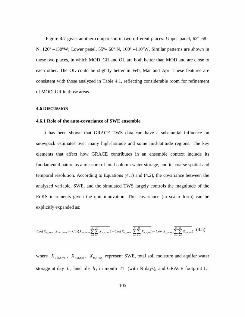
105
Figure 4.7 gives another comparison in two different places: Upper panel, 62º–68 º
N, 120º –130ºW; Lower panel, 55º– 60º N, 100º –110ºW. Similar patterns are shown in
these two places, in which MOD_GR and OL are both better than MOD and are close to
each other. The OL could be slightly better in Feb, Mar and Apr. These features are
consistent with those analyzed in Table 4.1, reflecting considerable room for refinement
of MOD_GR in those areas.
4.6 DISCUSSION
4.6.1 Role of the auto-covariance of SWE ensemble
It has been shown that GRACE TWS data can have a substantial influence on
snowpack estimates over many high-latitude and some mid-latitude regions. The key
elements that affect how GRACE contributes in an ensemble context include its
fundamental nature as a measure of total column water storage, and its coarse spatial and
temporal resolution. According to Equations (4.1) and (4.2), the covariance between the
analyzed variable, SWE, and the simulated TWS largely controls the magnitude of the
EnKS increments given the unit innovation. This covariance (in scalar form) can be
explicitly expanded as:
),(),(),(),(1 1
,,,,1 1
,,,,1 1
,,,,,1,1,, ∑∑∑∑∑∑= == == =
++=N
ti
M
liwalitiSWElt
N
ti
M
liSMlitiSWElt
N
ti
M
liSWElitiSWEltTWSLTSWElt XXCovXXCovXXCovXXCov (4.5)
where SWElitiX ,, , SMlitiX ,, , walitiX ,, represent SWE, total soil moisture and aquifer water
storage at day ti , land tile li , in month 1T (with N days), and GRACE footprint L1

106
(with M model grids), respectively. TWSLTX ,1,1 represents monthly (T1) average TWS
over L1. The symbol ∑∑ represents spatial and temporal averaging. The other
symbols have the same meaning as before. Here the decomposition of TWS neglects
canopy snow for simplicity. If further simplify equation (4.5) by only considering zero-
lag covariance parts of the second and third terms on the right side, it becomes
),(),(),(),( ,,,,,,,,1 1
,,,,,1,1,, waltSWEltSMltSWElt
N
ti
M
liSWElitiSWEltTWSLTSWElt XXCovXXCovXXCovXXCov ++≈ ∑∑
= =
(4.6)
Although incomplete, this expression provides a first-order estimate of the covariance
between daily SWE at any grid and the GRACE data, in particular for the accumulation
season. It assumes that soil moisture and groundwater anomalies are temporally and
spatially not well connected to the SWE anomaly before snow melts (a separate
calculation of the lagged correlation between SWE and the other two TWS components
supports this assumption, but is not shown here).
Figure 4.8 provides a monthly composite description of the cross-correlation
between SWE and the other two TWS components (the second and third terms in the
right side of equation (4.6)) in February, 2003; other months before strong melting show
similar results. Only in those colored areas, is there a significant correlation (p value <
5%) for more than two days in February. It is shown that over most of the domain both
correlation fields are not significant for a majority of days within that month. This
implies that the auto-correlation of SWE (the first term on the right side of equation (4.6))
largely determines the magnitude of GRACE information that can be utilized by CLM.
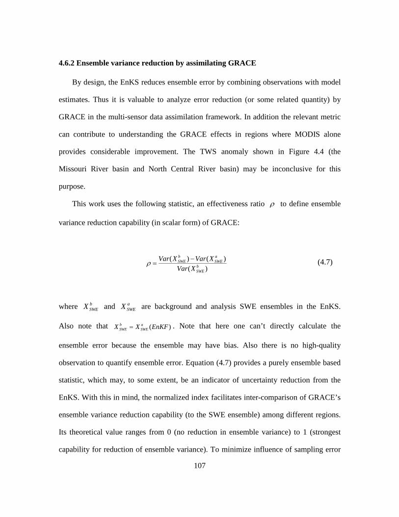
107
4.6.2 Ensemble variance reduction by assimilating GRACE
By design, the EnKS reduces ensemble error by combining observations with model
estimates. Thus it is valuable to analyze error reduction (or some related quantity) by
GRACE in the multi-sensor data assimilation framework. In addition the relevant metric
can contribute to understanding the GRACE effects in regions where MODIS alone
provides considerable improvement. The TWS anomaly shown in Figure 4.4 (the
Missouri River basin and North Central River basin) may be inconclusive for this
purpose.
This work uses the following statistic, an effectiveness ratio ρ to define ensemble
variance reduction capability (in scalar form) of GRACE:
)(
)()(bSWE
aSWE
bSWE
XVar
XVarXVar −=ρ (4.7)
where bSWEX and a
SWEX are background and analysis SWE ensembles in the EnKS.
Also note that )(EnKFXX aSWE
bSWE = . Note that here one can’t directly calculate the
ensemble error because the ensemble may have bias. Also there is no high-quality
observation to quantify ensemble error. Equation (4.7) provides a purely ensemble based
statistic, which may, to some extent, be an indicator of uncertainty reduction from the
EnKS. With this in mind, the normalized index facilitates inter-comparison of GRACE’s
ensemble variance reduction capability (to the SWE ensemble) among different regions.
Its theoretical value ranges from 0 (no reduction in ensemble variance) to 1 (strongest
capability for reduction of ensemble variance). To minimize influence of sampling error

108
in calculating ρ with equation (4.7), the daily river basin averaged values of ρ has
been derived. Figure 4.9 provides the results for two river basins, the Mackenzie and
North Central, from Jan, 2002 to Jun, 2002. ρ in the Mackenzie River basin is
systematically larger than that at mid-latitudes, and its average effectiveness ratio can
reach 25% in April, but decreases in the melting season when the MODIS capability
returns. In the North Central River basin this ratio is consistently below 10% and without
evident seasonal variation. Other boreal forest, tundra (compared to the Mackenzie River
basin) and mid-latitude flat regions (compared to the North Central River basin) have
similar patterns as shown here. However, results in mountainous regions are less
consistent. It is argued that ρ (for a large basin average) is also a function of the spatial
correlation structure of the MODIS updated ensemble within the GRACE footprint,
considering the spatial aggregation nature of GRACE. Further explanation of spatial and
seasonal variations of ρ is the subject of continued research.
4.7 CONCLUDING REMARKS
This study develops a continental scale multi-sensor snow data assimilation system
that assimilates both GRACE TWS and MODIS SCF information into CLM with the
EnKS and EnKF, respectively. Through this new framework, various deficiencies
associated with MODIS-only data assimilation are effectively corrected domain wide.
These improvements result from the unique information from GRACE, which provides
complementary constraints on the ensemble simulation for various climatic and
geographical locations. In addition, in those regions where MODIS performs adequately,
inclusion of GRACE TWS information does not degrade the estimates, further indicating

109
robustness of this joint assimilation system. Comparison of MOD_GR and OL reveals
more complex patterns. In the North Central, Missouri, and Saint Lawrence river basins,
MOD_GR is consistently better than OL. In Fraser and Yukon river basins, MOD_GR is
better than or comparable to OL. In the Mackenzie, Churchill & Nelson river basins OL
can have comparable or better performance than MOD_GR. These features demonstrate a
need to improve the GRACE data assimilation approach, including improved
characterization of GRACE bias and error variance.
I also found that measurement of total column water storage (integrating several
water storage components), and the coarse spatial and temporal resolution of GRACE
may both benefit and complicate the task of estimating SWE. The impacts of these
characteristics on the EnKS update deserve further investigation. Advantages of the finer
resolution of MODIS data in the multi-sensor system may need more detailed analyses in
order to better characterize the different features associated with each data type and their
interaction in the multi-sensor data assimilation framework.

110
Table 4.1 The mean absolute error (MAE) of monthly SWE (mm) from Jan to Jun at eight river basins in North America for three experiments. The superscripts represent that a specific experiment has significantly lower MAE (t-test, p-value < 0.01) in associated river basin and month than some of its counterparts. In particular, (a) - MOD_GR MAE is significantly lower than that of both MOD and Open Loop; (b) - MOD_GR MAE is only significantly lower than MOD; (c) - MOD_GR MAE is only significantly lower than Open Loop; (d)- Open_Loop MAE is significantly lower than that of both MOD and MOD_GR; (e) – Open Loop MAE is only significantly lower than MOD.
Columbia Jan Feb Mar Apr May Jun MOD_GR 34.2 48.6 48.1 36.2 27.4 2.4
MOD 36.9 46.1 47.0 32.8 24.8 4.0 Open_Loop 38.6 50.0 53.2 38.3 26.0 2.5 Fraser MOD_GR 53.3(b) 68.8(b) 89.3(a) 116.2(b) 62.1(a) 12.6(a)
MOD 62.4 86.5 104.1 137.2 68.2 30.9 Open_Loop 50.7(e) 74.9 103.0 126.8 86.0 21.6 Saint Lawrence MOD_GR 12.6(a) 18.2(a) 23.8(a) 32.8(a) 12.1(a) 2.2
MOD 23.1 29.1 36.5 47.2 21.8 4.1 Open_Loop 37.8 35.3 50.8 68.2 22.6 2.0 Mackenzie MOD_GR 27.7(a) 23.3(a) 26.5(a) 67.8(b) 36.3(b) 8.8(b)
MOD 39.1 39.6 53.5 86.6 46.2 22.0 Open_Loop 46.5 37.8 41.7 58.89(e) 26.2(d) 4.7(e) Churchill & Nelson MOD_GR 21.6(b) 26.9(b) 42.1(b) 58.1(b) 6.2 1.9
MOD 36.2 36.9 69.2 82.6 6.2 2.6 Open_Loop 29.1 21.3(e) 36.1(e) 48.6(d) 6.3 1.3 Yukon MOD_GR 52.8(c) 46.2(a) 52.1(a) 58.6(b) 33.9(a) 26.1(b)
MOD 51.2 57.1 62.6 70.1 52.1 36.8 Open_Loop 63.1 62.4 68.3 56.2(e) 59.8 18.5(e) Missouri MOD_GR 18.0(c) 20.9(c) 12.9(c) 11.0 2.7 0.1
MOD 19.3 21.2 12.1 11.7 3.6 1.0 Open_Loop 27.6 29.6 21.3 10.2 2.7 0.1 North Central MOD_GR 19.8(c) 21.1(c) 15.6(c) 4.1 0.1 0.0
MOD 16.2 18.2 12.1 3.7 1.5 1.2 Open_Loop 26.2 26.4 21.8 3.3 0.1 0.0
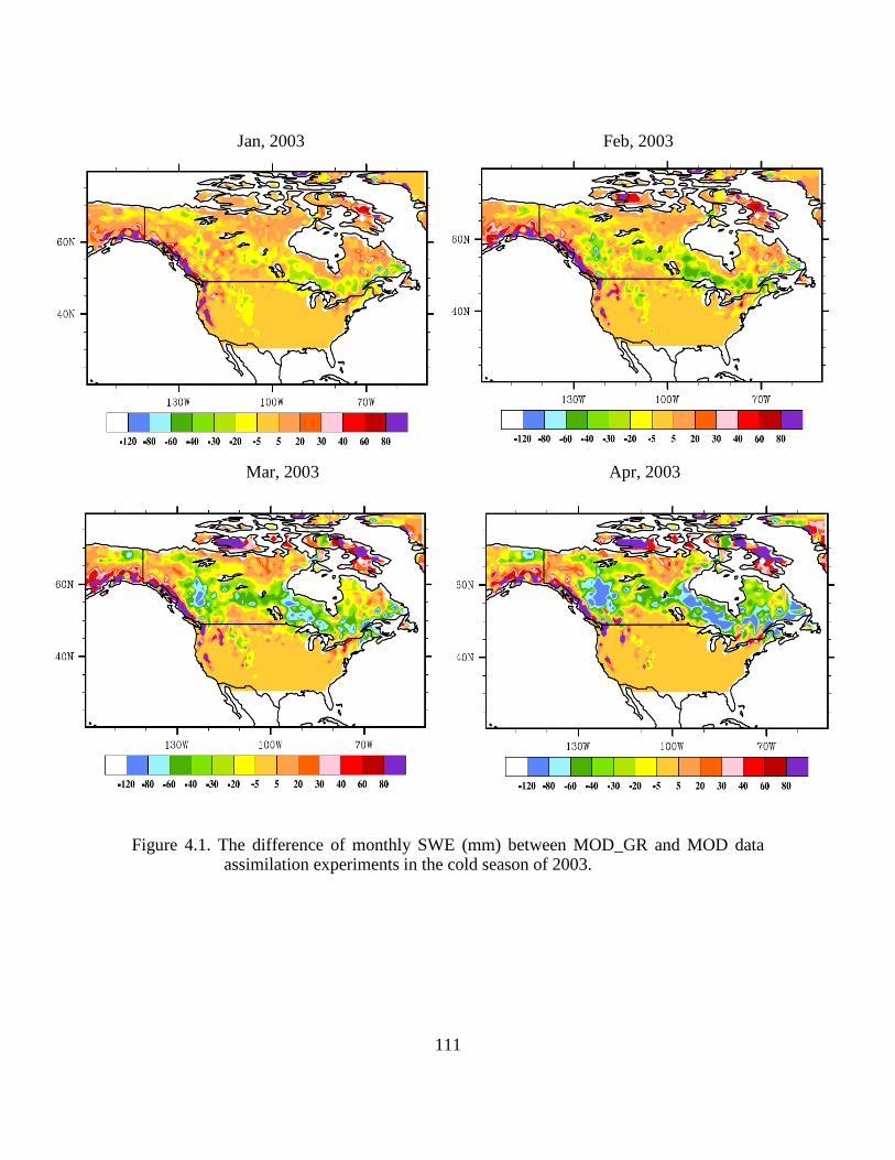
111
Jan, 2003 Feb, 2003 Mar, 2003 Apr, 2003
Figure 4.1. The difference of monthly SWE (mm) between MOD_GR and MOD data assimilation experiments in the cold season of 2003.
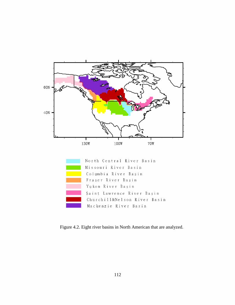
112
Figure 4.2. Eight river basins in North American that are analyzed.
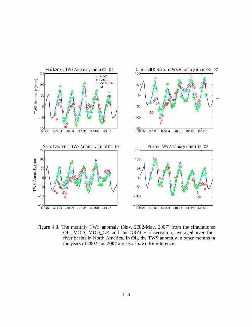
113
Figure 4.3. The monthly TWS anomaly (Nov, 2002-May, 2007) from the simulations: OL, MOD, MOD_GR and the GRACE observation, averaged over four river basins in North America. In OL, the TWS anomaly in other months in the years of 2002 and 2007 are also shown for reference.
TW
S A
no
mal
y (m
m)
T
WS
An
om
aly
(mm
)

114
Figure 4.4. Same as Figure 4.3., but for another four river basins in North America.
CMC (Apr) MOD_GR – CMC (Apr)
TW
S A
no
mal
y (m
m)
TW
S A
no
mal
y (m
m)
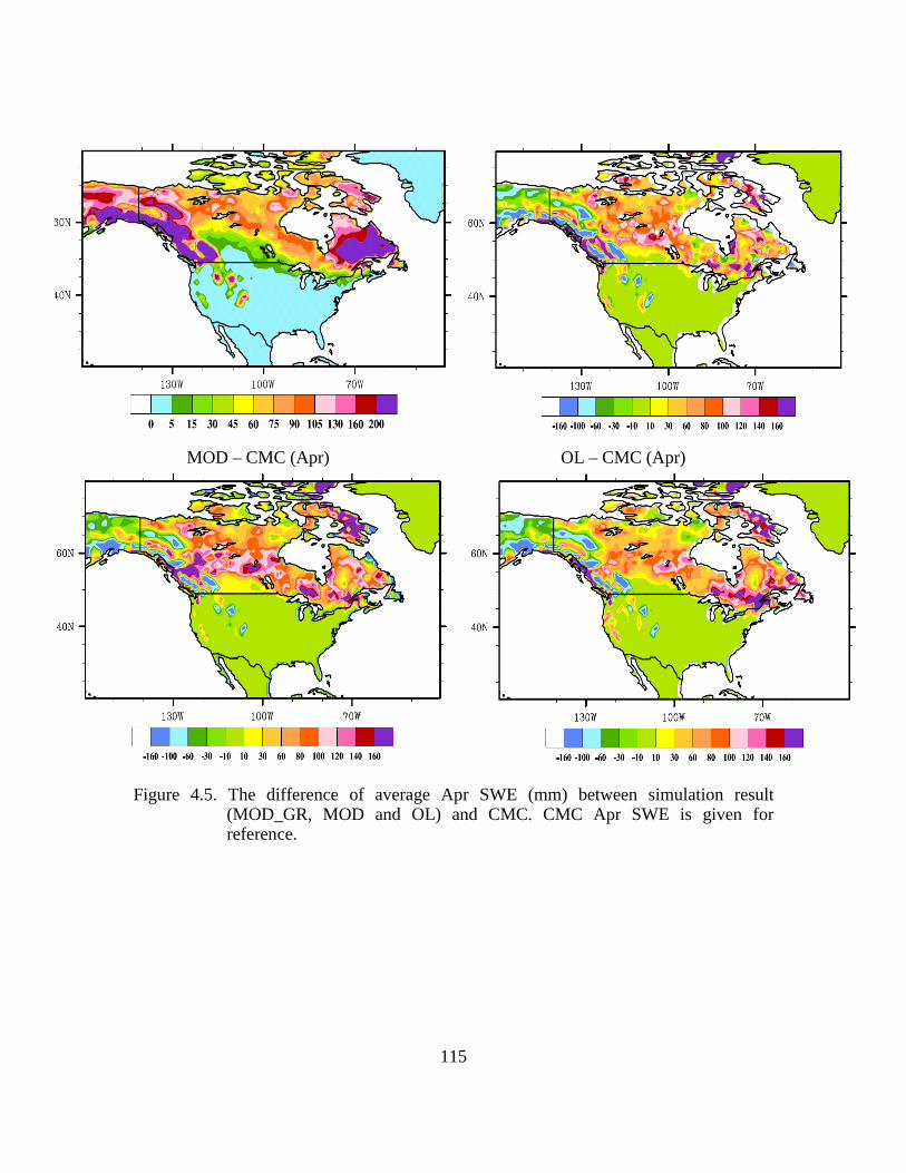
115
MOD – CMC (Apr) OL – CMC (Apr)
Figure 4.5. The difference of average Apr SWE (mm) between simulation result (MOD_GR, MOD and OL) and CMC. CMC Apr SWE is given for reference.

116
Figure 4.6. The climatological monthly mean SWE (mm) and snow depth (m) from Nov to Jun in two rectangular regions for the simulations (MOD, MOD_GR and OL), and the CMC long term observation data. Upper panel: (A) 51º–55 º N, 94º –85ºW; Lower panel: (B) 46º– 49º N, 98º –94ºW. See the rectangular boxes in Figure 4.8 for their locations.
SW
E (
mm
) S
WE
(m
m)
Sn
ow
Dep
th (
m)
Sn
ow
Dep
th (
m)

117
Figure 4.7. Same as in Figure 4.6 but for different locations. Upper panel: (C) 62º–68 º N,
120º –130ºW; Lower panel: (D) 55º– 60º N, 100º –110ºW. See the rectangular boxes in Figure 4.8 for their locations.
SW
E (
mm
) S
WE
(m
m)
Sn
ow
Dep
th (
m)
Sn
ow
Dep
th (
m)

118
Figure 4.8. In those colored grids, the number of the days in which the corresponding daily correlation (zero temporal and spatial lag) between (1) SWE and soil moisture (upper) (2) SWE and groundwater (lower) is significant (p value < 5%) exceeds two in February 2003.
Using a lower standard in the p-value test (e.g., p value < 10%) didn’t change these two colored maps significantly (remain almost same). Rectangular boxes in the upper panel are for Figure 4.6, 4.7.
C
D
A
B

119
Figure 4.9. The daily river basin averaged ρ (%) (equation (4.7)) from Jan to Jun 2003, for the Mackenzie River basin and the North Central River basin.
Mackenzie River basin
North Central River basin
(%)ρ

120
Chapter 5: Conclusions and future work
5.1 SUMMARY
The three studies described above are all devoted to developing improved
ensemble data assimilation approaches and strategies for estimating large-scale snowpack
properties (e.g., SWE, snow depth). Each study focuses on a specific aspect. Chapter 2
plays the role of “proof-of-concept” that first expands the EnKF SCF data assimilation to
a continental-scale. With this novel platform, new observation function and filter
characteristics are evaluated and interpreted on a new level. Following this initial test, a
more theoretically inclined topic is explored in Chapter 3, which tackles parameter and
model structure errors in the ensemble snow data assimilation system. Knowledge gained
from this chapter paves the way to more advanced large-scale snowpack estimation
practice in data-sparse areas where the true (or most appropriate) parameter and/or model
parameterization are poorly known. Chapter 4 concentrates on multi-sensor data
assimilation in the North American domain, where various observations are blended in an
approach incorporating both EnKF and EnKS. This study is partially motivated by
findings in Chapter 2 (the relatively poor performance in the boreal forest for MODIS
SCF data assimilation), and the comparison and contrast of these two studies leads to
valuable ramifications for large-scale ensemble snow data assimilation.
The major original findings and conclusions in each chapter are summarized
below.
In Chapter 2 it is demonstrated that MODIS SCF observation can be used to
estimate SWE at a continental-scale (North American) more precisely through the EnKF
121
approach. The potential of a newly developed SCF observation function has been
assessed, which shows that it can fit the specific needs of large-scale SWE estimation.
The data assimilation performance is found to be region dependent, where the climatic
and geographic (e.g., topography and vegetation) features can play an important role. The
largest improvements of EnKF experiment are in the mountainous West, the Northern
Great Plains, and the West and East Coast regions. In given areas, the MODIS
assimilation run can reduce the error of Open Loop from twice the standard deviation
(calculated from climatology) to within one standard deviation. However, the MODIS
EnKF approach is shown to perform poorly in boreal forests. In addition, the EnKF
statistics (innovation mean and mean of normalized innovation variance) have been
calculated and interpreted at domain wide. It is found that in middle-latitude areas there
are significant bias and misrepresentation of model error.
In Chapter 3 two parameters, the melting exponent in a SCF parameterization and
liquid water holding capacity, have been used to mimic parameter error in the EnKF data
assimilation. In presence of parameter error, the error in SWE estimation could be 100+
mm with a low Nash-Sutcliffe efficiency (0.22 for ensemble mean simulation), even
though measurements are assimilated. Incorporation of parameter estimation in
traditional EnKF could increase Nash-Sutcliffe efficiency to 0.96 (with 0.98 the
theoretical limit) and significantly reduce the SWE error. The energy balance related
variables are also estimated more accurately when performing parameter estimation.
Another experiment reveals that parameter estimation could diverge in the presence of
model structural error. It is speculated that the structural problem can undermine the
observation’s capability of leading to stable parameter retrieval. In the perfect-model-
122
structure scenario, parameter estimation converges and is not affected by the change of
variance of the parameter ensemble.
In Chapter 4, snow areal extent related observations (MODIS SCF) and mass
related observations (GRACE TWS) are blended into CLM for SWE and snow depth
estimation. It is found that the integrated EnKF and EnKS approach can adequately cope
with different features in these two datasets, for example, the discrepancy in their spatial
and temporal scales. This GRACE/MODIS data assimilation run achieves a significantly
better performance than the MODIS only run in Saint Lawrence, Fraser, Mackenzie,
Churchill & Nelson, and Yukon river basins. These improvements demonstrate the value
of integrating complementary information for continental-scale snow estimation,
especially, by incorporating TWS observation from GRACE. In middle latitude river
basins (e.g., North Central and Missouri) the multi-sensor approach preserves the
advantages (compared with Open Loop) shown in the MODIS only run. Further analyses
show that the auto-correlation of the SWE ensemble largely controls the magnitude of
GRACE information that can be absorbed by CLM. Also the capacity of GRACE
observation in reducing the SWE ensemble variance (a surrogate of estimation error) is
assessed at river basin scale, with a first-order result showing that this capacity is larger
in high latitude flat areas than in middle latitude flat areas.

123
5.2 FUTURE WORK
There are many limitations and constraints revealed in the above investigations.
In general, research presented in this dissertation can be expanded and improved by
investigating the following issues.
(1) Characterization of observation error. In two satellite datasets involved studies
(Chapters 2 and 4), the observation errors are specified in a simple way which, in some
region and period, could significantly depart from the true value. MODIS SCF data may
have large uncertainties in forest and mountain areas, and GRACE TWS error may be
latitude dependent. In Chapter 4 it is hypothesized that, the simple treatment of TWS
error could be responsible for the indistinguishable or even degraded performance of
multi-sensor runs when compared to the Open Loop run over some high latitude areas. It
is recommended to incorporate spatially and temporally distributed estimates of
observation errors, and evaluate their impacts on data assimilation performance.
(2) Representation of spatial and temporal structures of large-scale meteorological
forcing errors. As highlighted in Crow and Van Loon (2006), accurate description of
forcing (or model) error magnitude could be paramount to a land data assimilation
system. Durand and Margulis (2006) also showed the importance of spatial covariance of
precipitation error in an ensemble snowpack estimation experiment. In Chapter 2, it is
found the forcing errors are misrepresented in middle latitude areas. In Chapter 4, the
auto-correlation of SWE is demonstrated to be important to GRACE information
absorption. This ensemble metric is a function of the spatial correlation structure of
forcing data (e.g., precipitation and temperature). That said, how to simulate these forcing
errors adequately at continental to hemispheric scale is not covered in this dissertation
124
and previous research. Solid precipitation data error might be linked to the feature of
large-scale frontal systems in winter. In addition, these forcing data errors are largely
related to the way they are generated (e.g., the production of reanalysis data through
blending multiple sources like satellite observation and coupled GCM simulation).
Therefore great efforts are needed to derive dependable algorithms that can better
quantify these forcing error structures.
(3) Adaptive filter algorithm that can more efficiently transform information in
satellite observation (e.g., GRACE TWS) to model simulation. This requirement is
related to the increasing computational demand when higher resolution LSMs are used in
snow data assimilation. My study reveals that the effectiveness of GRACE assimilation
might vary regionally, with given areas affected insignificantly. Also it might not be
necessary to assimilate MODIS SCF information at daily frequency considering the
memory of snow cover in given season and area. Although mechanisms that control the
regionally and temporally dependent filter performance are not yet clear, it can be
speculated that an adaptive approach that can automatically determine the application of
the EnKF could reduce both computational burden and sampling error. The EnKF update
(of given observations) may not need at particular places or periods because its expected
(theoretical) value is marginal. So it may be appropriate to adjust the size of areas (or
temporal interval) involved in the ensemble update for a particular observation.
(4) Assimilation of range-rate data from GRACE satellite. Considering the
limitations of current version of monthly GRACE TWS data (for example, the coarse
temporal and spatial resolution, and the aliasing problems), assimilating range-rate
variation along the satellite ground track could improve results. Range-rate data can form
125
local estimates of surface mass change near the ground track with variable temporal
sampling intervals, and have spatial coverage depending on the details of ground tracks.
These features potentially enable SWE estimation at high spatial and temporal
resolutions. An Observation System Simulation Experiment (OSSE) is desirable to fully
test the performance of range-rate data assimilation and the associated technical details.
(5) Generation of longer period (e.g., decadal) snowpack estimates using AVHRR
satellite data. Currently the snowpack estimates span only several years, which are
limited by the availability of MODIS and GRACE datasets. AVHRR provided SCF data
from 1970s (although at coarser spatial resolution than MODIS). Using the same EnKF
technology, these data can be assimilated to derive long-term snowpack estimates. These
estimates could be useful for a wide range of applications, especially for evaluating long-
term hydroclimatological change.
(6) Integration of ensemble snow data assimilation methods into coupled
meteorological and/or climate models. As indicated in Chapter 1, one reason for
developing snow products through data assimilation is to provide reliable boundary
conditions for meteorological and climate simulation. All three chapters demonstrate that
the characteristics (e.g., error magnitude) of SWE, snow depth and other snowpack
estimates are largely controlled by the model features, for example, its numerical
configuration, accuracy of parameters and structure, reliability of observational function,
etc. So the integration of ensemble snow data assimilation methods into the
meteorological and/or climate models (e.g., using the same LSM to assimilate
observation and simulate snowpack related boundary states and fluxes in GCM) is
promising to produce a seamless approach. Currently it is not clear how to develop a

126
computationally efficient way to achieve the above goal. There are further questions
about the benefit of this approach for intra-seasonal to seasonal atmospheric simulation.
The study toward this goal could be integrated into some community efforts that have
potentially far-reaching impacts and cover wide range of scales and areas. For example,
the Data Assimilation Research Testbed (DART) is a community facility for ensemble
data assimilation developed and maintained by the Data Assimilation Research Section
(DAReS) at the National Center for Atmospheric Research (NCAR). It includes multiple
comprehensive atmosphere and ocean general circulation models (GCMs) and modular
programming facility for ensemble data assimilation. The integration of the snow data
assimilation component into this community platform can characterize the effects of
optimized snow estimation to climate simulation.

127
Appendix
Abbreviations AMSR-E Advanced Microwave Scanning Radiometer-Earth AVHRR Advanced Very High Resolution Radiometer CLM Community Land Model EnKF Ensemble Kalman Filter EnKS Ensemble Kalman Smoother GCMs General Circulation Models GLDAS Global Land Data Assimilation System GRACE Gravity Recovery and Climate Experiment MODIS Moderate Resolution Imaging Spectroradiometer NCAR National Center for Atmosphere Research NDSI Normalized Difference of Snow Index NRCS Natural Resources Conservation Service OSSE Observation System Simulation Experiment PDO Pacific Decadal Oscillation PFTs Plant Functional Types PNA Pacific-North America (pattern) SCF Snow Cover Fraction SDC Snow Depletion Curve SNOTEL Snowpack Telemetry SWE Snow Water Equivalent VIS/IR Visible/Infrared
128
References
Aksoy A., F. Zhang, J. W. Nielsen-Gammon (2006), Ensemble-based simultaneous state
and parameter estimation in a two-dimensional sea breeze model. Mon. Weather Rev., 134, 2951-2970.
Anderson, E. A. (1976), A point energy and mass balance model of a snow cover, Office
of Hydrology, NOAA Tech. Rep. NWS 19. 150 pp, National Weather Service. Anderson, J. L. (2001), An ensemble adjustment Kalman filter for data assimilation,
Mon. Weather Rev., 129, 2884-2903. Andreadis K. M., D. P. Lettenmaier (2006), Assimilating remotely sensed snow
observations into a macroscale hydrology model, Adv. Water Resour., 29(6), 872-886.
Andreadis, K. M., D. Liang, L. Tsang, D. P. Lettenmaier, and E. G. Josberger, (2008)
Characterization of errors in a coupled snow hydrology-microwave emission model, J. Hydrometeorology (accepted)
Barnett T.P., J.C. Adam, and D.P. Lettenmaier (2005), Potential Impacts of a Warming
Climate on Water Availability in Snow-Dominated Regions, Nature, 438: 303-309
Barnett, T. P., L. Dumenil, U. Schlese, E. Roechner, and M. Latif (1989), The effect of
Eurasian snow cover on regional and global climate variations, J. Atmos. Sci., 46, 661–685.
Blöschl, G (1999), Scaling issues in snow hydrology, Hydrol. Processes, 13, 2149-2175. Bonan, K. W. Oleson, M. Vertenstein, S. Levis, X. B. Zeng, Y. J. Dai, R. E. Dickinson,
and Z. L. Yang (2002), The land surface climatology of the community land model coupled to the NCAR community climate model, J. Clim., 15, 3123–3149.
Brown, R. D., B. Brasnett, D Robinson (2003), Gridded North American monthly snow
depth and snow water equivalent for GCM evaluation, Atmosphere-Ocean, 41(1), 1-14.
Brubaker, K. L., M. Jasinski, A. T. Chang, and E. Josberger (2001), Interpolating sparse
surface measurements for calibration and validation of satellite-derived snow water

129
equivalent in Russian Siberia, in: Remote sensing and Hydrology 2000, edited by: Owe, M., Brubaker, K., Ritchie, J., and Rango, A., IAHS Publ. No. 267, 93–98.
Brubaker, K. L., R. T. Pinker, E. Deviatova (2005), Evaluation and comparison of
MODIS and IMS snow-cover estimates for the continental United States using station data, J. Hydrometeorol., 6(6), 1002-1017.
Burgers, G., P. J. van Leeuwen, and G. Evensen (1998), Analysis scheme in the
ensemble Kalman filter, Mon. Weather Rev., 126, 1719–1724. Canadian Snow Data CD-ROM (2000), (http://www.ccin.ca/datasets
/snowcd/docs/1999/DOCUMNTS/INTRO_E.HTM) Chen, J.L., C.R. Wilson, B.D Tapley, D.D. Blankenship, D. Young, Antarctic Regional
Ice Loss Rates From GRACE (2008), Earth and Planetary Science Letters, Vol. 266/1-2, doi: 10. 1016/j.epsl.2007.
Clark, M. P., A. G. Slater, A. P. Barrett, L. E. Hay, G. J. McCabe, et al. (2006),
Assimilation of snow covered area information into hydrologic and land-surface models, Adv. Water Resour., 29, 1209-1221.
Clark, M. P., and J. A. Vrugt (2006), Unraveling uncertainties in hydrologic model
calibration: Addressing the problem of compensatory parameters, Geophys. Res. Lett., 33, L06406, doi:10.1029/2005GL025604
Clark, M. P., A. G. Slater, D. E. Rupp, R. A. Woods, J. A. Vrugt, H. V. Gupta, T.
Wagener, L. E. Hay (2008), Framework for Understanding Structural Errors (FUSE): A modular framework to diagnose differences between hydrological models, Water Resour. Res., 44, W00B02, doi:10.1029/2007WR006735.
Crow, W. T. (2003), Correcting land surface model predictions for the impact of
temporally sparse rainfall rate measurements using an ensemble Kalman filter and surface brightness temperature observations, J. Hydrometeorol., 4, 960–973.
Crow, W. T., E. V. Loon (2006), Impact of Incorrect Model Error Assumptions on the
Sequential Assimilation of Remotely Sensed Surface Soil Moisture, J. Hydrometeorol., 7, 421-433.
De Lannoy GJM, Reichle RH, Houser PR, et al. (2007), Correcting for forecast bias in
soil moisture assimilation with the ensemble Kalman filterSource: Water Resour. Res., 43, W09410.
Dee, D. P.(1995), On-line estimation of error covariance parameters for atmospheric data
assimilation, Mon. Weather Rev., 123, 1128-1145.

130
Deems, J.S., S.R. Fassnacht, and K.J. Elder (2008), Interannual consistency in fractal snow depth patterns at two Colorado mountain sites, J. Hydrometeorol, 9(5), 977 - 988.
Dingman, S. L. (2002), Physical Hydrology, Prentice Hall (2nd edition). Donald, J. R., E. D. Soulis, and N. Kouwen, (1995), A land cover based snow cover
representation for distributed hydrologic models, Water Resour. Res., 31, 995–1009.
Dong J. R., J. P Walker, P. R. Houser (2005), Factors affecting remotely sensed snow
water equivalent uncertainty (2005), Remote Sens. Environ., 97, 68-82. Dong, J., J. P. Walker, P. R. Houser, and C. Sun (2007), Scanning multichannel
microwave radiometer snow water equivalent assimilation, J. Geophys. Res., 112, D07108, doi:10.1029/2006JD007209.
Dunne S, Entekhabi D (2005), An ensemble-based reanalysis approach to land data
assimilation , Water Resour. Res., 41. WR003449 Dunne S, Entekhabi D (2006), Land surface state and flux estimation using the ensemble
Kalman smoother during the Southern Great Plains 1997 field experiment, Water Resour. Res.,,42. doi:10,1029/2005WR004334
Durand M, S. A. Margulis (2006), Correcting first-order errors in snow water equivalent
estimates using a multifrequency, multiscale radiometric data assimilation scheme, J. Geophys. Res., 112.
Durand M, S. A. Margulis (2006), Feasibility test of multifrequency radiometric data
assimilation to estimate snow water equivalent, J. Hydrometeorol., 7, 443-457. Durand M, S. A. Margulis (2007), Correcting first-order errors in snow water equivalent
estimates using a multifrequency, multiscale radiometric data assimilation scheme, J. Geophys. Res., 112, D13121, doi:10.1029/2006JD008067.
Dyer, L. J., and T. L. Mote, 2006: Spatial variability and trends in snow depth over North
America. Geophys. Res. Lett., 33, L16503, doi:10.1029/2006GL027258 Epstein, E. S., Stochastic dynamic prediction (1969), Tellus, Series. A, 21, 739-759, Etchevers P., E. Martin, R. Brown, C. Fierz, Y. Lejeune, E. Bazile, A. Boone, Y.-J. Dai,
R. Essery, A. Fernandez, Y. Gusev, R. Jordan, V. Koren, E. Kowalczyck, R. Nasonova, D. Pyles, A. Schlosser, A. B. Shmakin, T. G. Smirnova, U. Strasser, D. Verseghy, T. Yamazaki, Z.-L. Yang (2002), SnowMiP: An intercomparison of snow models : first results. Proceedings of the International Snow Science Workshop, Penticton, Canada.
131
Evensen, G. (1994), Sequential data assimilation with a nonlinear QG model using Monte
Carlo methods to forecast error statistics, J. Geophys. Res., 99, 10143–10 162. Evensen, G. (2003), The ensemble Kalman filter: Theoretical formulation and practical
implementation, Ocean Dynamics, 53, 343–367. Foster, J. L., C.J. Sun, J. P. Walker, R. Kelly, A. Chang, J.R. Dong, and H. Powell
(2005), Quantifying the uncertainty in passive microwave snow water equivalent observations, Remote Sens. Environ., 94, 187-203.
Frei, A and G. Gong (2005), Decadal to Century Scale Trends in North American Snow
Extent in Coupled Atmosphere-Ocean General Circulation Models. Geophys. Res. Lett, 32, L18502, doi: 10.1029/2005GL023394.
Gao, H., E. F. Wood, M. Drusch, and M. F. Mccabe (2007), Copula-Derived Observation
Operators for Assimilating TMI and AMSR-E Retrieved Soil Moisture into Land Surface Models, J. Hydrometeorol. , 8(3), 413-429.
Ge, Y. and G. Gong (2009), North American Snow Depth and Climate Teleconnection
Patterns. Journal of Climate, 22, 217-233 Gong et al. (2003), Modeled Northern Hemisphere Winter Climate Response to Realistic
Siberian Snow Anomalies, J. Clim., 16, 3917-3931. Gong, G., D. Entekhabi and J. Cohen (2003). Relative Impacts of Siberian and North
American Snow Anomalies on the Northern Hemisphere Mode. Geophys. Res. Lett, 30(16), 1848, doi: 10.1029/2003GL017749
Grody NC, Basist AN (1996), Global identification of snowcover using SSM/I
measurements, IEEE Trans. Geosci. Remote Sens, 34(1), 237-49. Hall D. K., G. A. Riggs, V. V. Salomonson, et al (2002), MODIS snow-cover products,
Remote Sens. Environ., 83(1-2), 181-194. Hall, D.K., G. A. Riggs (2007), Accuracy assessment of the MODIS snow products.
Hydrol. Processes, 21, 1534-1547 Hamill, T. M. (2006), Ensemble-based atmospheric data assimilation, Predictability of
Weather and Climate, 124-156, Cambridge Press. Houser, P. R., et al. (1998), Integration of soil moisture remote sensing and hydrologic
modeling using data assimilation, Water Resour. Res., 34, 3405-3420.

132
Klein, A. G., A. C. Barnett (2003), Validation of daily MODIS snow maps of the Upper Rio Grande River Basin for the 2000-2001 snow year, Remote Sens. Environ., 86, 162-176.
Liston, G. E. (2004), Representing subgrid snow cover heterogeneities in regional and
global models, J. Clim., 17, 1381-1397. Liu, Y., and H. V. Gupta (2007), Uncertainty in hydrologic modeling: Toward an
integrated data assimilation framework, Water Resour. Res., 43, W07401, doi:10.1029/2006WR005756.
Luce, C. H., D. G Tarboton (2004), The application of depletion curves for
parameterization of sub-grid variability of snow, Hydrol. Processes, 18, 1409-1422. Luce, C. H., D. G. Tarboton, C. R Cooley (1999), Sub-grid parameterization of snow
distribution for an energy and mass balance snow cover model, Hydrol. Processes, 13, 1921-1933.
Renzullo, L. J., D. J. Barrett, A. S. Marks, M. J. Hill, J. P. Guerschman, Q. Z. Mu, S. W.
Running (2008), Multi-sensor model-data fusion for estimation of hydrologic and energy flux parameters, Remote Sens. Environ., 112, 1306-1319.
Margulis S.A., D. B. McLaughlin, D. Entekhabi, S. Dunne (2002), Land data assimilation
and estimation of soil moisture using measurements from the Southern Great Plains 1997 Field Experiment, Water Resour. Res., 38, 1299.
Markus T., D. C. Powell, J. R. Wang (2006), Sensitivity of passive microwave snow
depth retrievals to weather effects and snow evolution, IEEE Trans. Geosci. Remote Sens, 44(1), 68-77.
McLaughlin, D. B. (2002), An integrated approach to hydrologic data assimilation:
Interpolation, smoothing, and filtering, Adv. Water Resour., 25, 1275–1286. Moradkhani, H, S. Sorooshian, H. V. Gupta, P. R. Houser (2005), Dual state–parameter
estimation of hydrological models using ensemble Kalman filter, Adv. Water Resour, 28(2),
Mote, T., A. Grundstein, D. Leathers, and D. Robinson (2003), A comparison of
modeled, remotely sensed, and measured snow water equivalent in the northern Great Plains, Water Resour. Res., 39(8), 1209, doi:10.1029/2002WR001782.
Nijssen, B., D. P. Lettenmaier (2004), Effect of precipitation sampling error on simulated
hydrological fluxes and states: Anticipating the Global Precipitation Measurement satellites, J. Geophys. Res., 109(D2), doi:10.1029/2003JD003497.

133
Niu, G.-Y., Z.-L. Yang, R.E. Dickinson, and L.E. Gulden (2005), A simple TOPMODEL-based runoff parameterization (SIMTOP) for use in GCMs, J. Geophys. Res., 110, doi:10.1029/2005JD006111.
Niu, G.-Y. and Z.-L. Yang (2006), Effects of frozen soil on snowmelt runoff and soil
water storage at a continental-scale, J. Hydrometeorol. , 7 (5), 937-952. Niu, G.Y., K.-W. Seo, Z.-L. Yang, C. R. Wilson, H. Su, Chen, J.L., M. Rodell (2007),
Retrieving Snow Mass from GRACE Terrestrial Water Storage Change with a Land Surface Model, Geophys. Res. Lett., 34, L15704, doi:10.1029/2007GL030413.
Niu, G.Y., Z.-L. Yang, R. E. Dickinson, et al. (2007), Development of a simple
groundwater model for use in climate models and evaluation with Gravity Recovery and Climate Experiment data, J. Geophys. Res., 112, D07103.
Niu, G.-Y., Z.-L. Yang (2007), An observation-based snow cover fraction formulation
and evaluation over large North American river basins, J. Geophys. Res, 112, D21101, doi:10.1029/2007JD008674
Oleson, K. W., Y. Dai et al. (2004), Technical description of the Community Land Model
(CLM), NCAR Technical Note NCAR/TN-461+STR, 173 pp., National Center for Atmospheric Research, Boulder, CO
Oleson, K. W., Y. Dai et al. (2004), Technical description of the Community Land Model
(CLM), NCAR Technical Note NCAR/TN-461+STR, 173 pp., National Center for Atmospheric Research, Boulder, CO.
Pomeroy, J. W., and D. M. Gray, K. R. Shook, B. Toth, R. L. H. Essery, A. Pietroniro, and N. Hedstrom, (1998), An evaluation of snow accumulation and ablation
processes for land surface modeling, Hydrol. Processes, 12, 2339–2367. Reichle, R. H., D. B. McLaughlin, and D. Entekhabi (2002), Hydrologic data assimilation
with the ensemble Kalman filter, Mon. Weather Rev., 130, 103–114. Reichle, R. H., and R. D. Koster (2003), Assessing the impact of horizontal error
correlations in background fields on soil moisture estimation, J. Hydrometeorol., 4, 1229–1242.
Reichle, R. H., and R. D. Koster (2004), Bias reduction in short records of satellite soil
moisture, Geophys. Res. Lett., 31, doi:10.1029/2004GL020938. Reichle RH, W. T. Crow, C. L. Keppenne, An adaptive ensemble Kalman filter for soil
moisture data assimilation (2008), Water Resour. Res., 44, doi: 10. 1029/2007WR006357
134
Renzullo L. J. et al. (2008),Multi-sensor model-data fusion for estimation of hydrologic and energy flux parameters, Remote Sensing of Environment 112, 1306–1319
Rodell, M., and Coauthors, 2004: The global land data assimilation system, Bull. Am.
Meteorol. Soc., 85, 381–394. Rodell, M., and P. R. Houser (2004), Updating a land surface model with MODIS-
derived snow cover, J. Hydrometeorol., 5, 1064–1075. Rodell, M., J.S. Famiglietti, J.L. Chen, S. Seneviratne, P. Viterbo, and S. Holl, River
basin water budget estimates of evapotranspiration using GRACE derived terrestrial water storage with observation based precipitation and runoff, Geophys. Res. Lett., Vol. 31, No. 20, L20807, 10.1029/2004GL021104.
Rosero, E., Z.-L. Yang, T. Wagener, L. E. Gulden, S. Yatheendradas, and G.-Y. Niu,
(2009), Quantifying parameter sensitivity, interaction and transferability in hydrologically enhanced versions of Noah-LSM over transition zones, J. Geophys. Res.
Simic et al. (2004), Validation of VEGETATION, MODIS, and GEOS + SSM/I snow-
cover products over Canada based on surface snow depth observations. Hydrol. Processes, 18(6), 1089-1104.
Slater, A. G., and Clark, M P. (2006), Snow data assimilation via an ensemble Kalman
Filter, J. Hydrometeorol., 7, 3–22. Shook, K., and D. M. Gray, (1996), Small-scale spatial structure of shallow snowcovers.
Hydrol. Processes, 10, 1283–1292. Souma, K., Yu. Q. Wang, (2009), Improved simulation of the East Asian Summer
Monsoon rainfall with satellite-derived snow water equivalent data, Mon. Weather Rev., 137, 1790-1804.
Su, H., Z. L. Yang, G. Y. Niu, R. E. Dickinson (2008), Enhancing the estimation of
continental-scale snow water equivalent by assimilating MODIS snow cover with the ensemble Kalman filter, J. Geophys. Res., 113, 10.1029/2007JD009232.
Syed, T.H., J. S. Famiglietti, M. Rodell, J.L. Chen, C.R. Wilson, Analysis of Terrestrial
Water Storage Changes from GRACE and GLDAS (2008), Water Resour. Res.,, 44, W02433, doi:10.1029/2006WR005779.
Tedesco, M. and E. J. Kim (2006), Intercomparison of electromagnetic models for
passive microwave remote sensing of snow, IEEE Trans. Geosci. Remote Sens., 44(10), 2652-2666.

135
Tedesco, M., E.J. Kim, A. W. England, R. de Roo and J. P. Hardy (2006), Brightness temperatures of snow melting/refreezing cycles: Observations and modeling using a multilayer dense medium theory-based model, IEEE Trans. Geosci. Remote Sens., 44(12), 3563-3573.
Tsang, L., J. Pan, D. Liang, Z. X. Li, D. W. Cline, Y. H., Tan (2007), Modeling Active
Microwave Remote Sensing of Snow Using Dense Media Radiative Transfer (DMRT) Theory With Multiple-Scattering Effects, IEEE Trans. Geosci. Remote Sens, 45.
Vrugt, C.G.H.Diks, W. Bouten, H.V. Gupta, and J.M. Verstraten, Improved treatment of
uncertainty in hydrologic modeling (2005), Combining the strengths of global optimization and data assimilation, Water Resour. Res., 41(1), W01017, doi:10.1029/2004WR003059,
Yang, F., A. Kumar, W. Wang, H. H. Juang, and M. Kanamitsu (2001), Snow-albedo
feedback and seasonal climate variability over North America, J. Clim., 14, 4245–4248.
Yang, Z.-L., R. E. Dickinson, A. Robock and K.Y. Vinnikov (1997), Validation of the
snow sub-model of the Biosphere-Atmosphere Transfer Scheme with Russian snow cover and meteorological observational data, J. Clim., 10, 353-373.
Yang, Z.-L. and G.-Y. Niu (2003), The Versatile Integrator of Surface and Atmosphere
Processes (VISA) Part 1: Model description, Global and Planetary Change, 38, 175-189
Zaitchik, B. F., M. Rodell, R. H. Reichle(2008), Assimilation of GRACE terrestrial water
storage data into a Land Surface Model: Results for the Mississippi River basin, J. Hydrometeorol., 9, 535-548.

136
Vita
Hua Su was born in Changsha, China. He earned an B.E. in Hydraulic Engineering
from Tsinghua University in 2000. He received an M.S. in Hydrology and Water
Resources from Tsinghua University in 2002.
Permanent address: 7205 Hart Lane 2009, Austin, TX 78731
This dissertation was typed by the author.

137