copyright by mikhail yuryevich bilenko 2006ml/papers/marlin-dissertation-06.pdf · the dissertation...
TRANSCRIPT

Copyright
by
Mikhail Yuryevich Bilenko
2006
The Dissertation Committee for Mikhail Yuryevich Bilenko
certifies that this is the approved version of the following dissertation:
Learnable Similarity Functions and Their Application
to Record Linkage and Clustering
Committee:
Raymond J. Mooney, Supervisor
William W. Cohen
Inderjit S. Dhillon
Joydeep Ghosh
Peter H. Stone
Learnable Similarity Functions and Their Application
to Record Linkage and Clustering
by
Mikhail Yuryevich Bilenko, B.S.; M.S.
Dissertation
Presented to the Faculty of the Graduate School of
The University of Texas at Austin
in Partial Fulfillment
of the Requirements
for the Degree of
Doctor of Philosophy
The University of Texas at Austin
August 2006

To my dear grandparents

Acknowledgments
I am indebted to many people for all the help and support I received over the past six years.
Most notably, no other person influenced me as much as my advisor, Ray Mooney. Ray has
been a constant source of motivation, ideas, and guidance. His encouragement to explore
new directions while maintaining focus has kept me productive and excited about research.
Ray’s passion about science, combination of intellectual depth and breadth, and great per-
sonality have all made working with him a profoundly enriching and fun experience.
Members of my committee, William Cohen, Inderjit Dhillon, Joydeep Ghosh and
Peter Stone, have provided me with many useful ideas and comments. William’s work has
been a great inspiration for applying machine learning methods to record linkage, and I am
very grateful to him for providing detailed feedback and taking the time to visit Austin. In-
derjit and Joydeep gave me a terrific introduction to data mining in my first year in graduate
school, and have had a significant influence on me through their work on clustering. I deeply
appreciate Peter’s helpful insights, encouragement and advice on matters both related and
unrelated to this research.
I have been lucky to work with several wonderful collaborators. Throughout my
graduate school years, Sugato Basu has been the perfect partner on countless projects, a
great sounding board, and a kind friend. Talking to Arindam Banerjee has always been
both eye-opening and motivating. During my internship at Google, working with Mehran
Sahami has been enlightening and exciting, and I have appreciated Mehran’s kindness and
wisdom on many occasions. Exploring several new research directions in the past year with
v
Beena Kamath, Peng Bi, Tuyen Huynh, Maytal Saar-Tsechanskyand Duy Vu has been a
stimulating finish for my graduate career.
My academic siblings in the Machine Learning Group are a wonderful clever bunch
who have been a joy to be around. I am most grateful to Prem Melville for his trusty
friendship, razor-sharp wit, and reliable company in all sorts of places at all sorts of hours;
doing science(and not-quite-science) side-by-side with Prem has been a highlight of the
past years. Lily Mihalkova and Razvan Bunescu have been essential in providing much
needed moral support in the office when it was most needed in the final stretch. Sugato,
Prem, Lily, Razvan, Un Yong Nahm, John Wong, Ruifang Ge, Rohit Kate, and Stewart
Yang have been always ready to help with papers, practice talks and anything else in work
and life, and I hope to see them often for years to come.
A number of UTCS staff members have provided me their supportduring the past
six years. The administrative expertise of Stacy Miller, Gloria Ramirez and Katherine Utz
has been much appreciated on many occasions. My life has beenmade much easier by the
friendly department computing staff who have provided a well-oiled and smoothly running
environment for all the experiments in this thesis.
I am grateful to many fellow UTCS grad students for their intellectually stimulat-
ing camaraderie. Joseph Modayil has been a great friend, a dream roommate, and baker
extraordinaire whose editing skills have been invaluable anumber of times, including the
present moment. Yuliya Lierler’s warm friendship has brightened many days, and seeing
her in Austin after her German sojourn is a perfect graduation gift. The company of Aniket
Murarka, Amol Nayate, Nalini Belaramani, Patrick Beeson, Nick Jong, Alison Norman and
Serita Nelesen has been a precious pleasure on too many occasions to count, and I hope I
will enjoy it in the future as often as possible.
My friends outside computer science have made my years in Austin a fantastic
experience. From climbing trips to live music shows to random coffeeshop jaunts, they
have given my life much-needed balance and spice.
vi

My road to this point would not be possible without the peopleI love. My sister Na-
talia, parents Olga and Yury, and grandparents Tamara Alexandrovna, Nina Alexandrovna,
Alexander Mikhailovich and David Isakovich have always given me their unconditional
love and support. My family has inspired me, encouraged me, and helped me in every
possible way, and there are no words to express my gratitude.Sandra, Dick, Gretchen and
Grant Fruhwirth selflessly opened their home to me when I firstcame to the US, have been
by my side during my college years, and will always be family to me. Finally, I thank Anna
Zaster for making my life complete. I would not be happy without you.
The research in this thesis was supported by the University of Texas MCD Fellow-
ship, the National Science Foundation under grants IIS-0117308 and EIA-0303609, and a
Google Research Grant.
M IKHAIL YURYEVICH BILENKO
The University of Texas at Austin
August 2006
vii
Learnable Similarity Functions and Their Application
to Record Linkage and Clustering
Publication No.
Mikhail Yuryevich Bilenko, Ph.D.
The University of Texas at Austin, 2006
Supervisor: Raymond J. Mooney
Many machine learning and data mining tasks depend on functions that estimate similarity
between instances. Similarity computations are particularly important in clustering and
information integration applications, where pairwise distances play a central role in many
algorithms. Typically, algorithms for these tasks rely on pre-defined similarity measures,
such as edit distance or cosine similarity for strings, or Euclidean distance for vector-space
data. However, standard distance functions are frequentlysuboptimal as they do not capture
the appropriate notion of similarity for a particular domain, dataset, or application.
In this thesis, we present several approaches for addressing this problem by em-
ploying learnablesimilarity functions. Given supervision in the form of similar or dis-
viii
similar pairs of instances, learnable similarity functions can be trained to provide accurate
estimates for the domain and task at hand. We study the problem of adapting similarity
functions in the context of several tasks: record linkage, clustering, and blocking. For each
of these tasks, we present learnable similarity functions and training algorithms that lead to
improved performance.
In record linkage, also known as duplicate detection and entity matching, the goal
is to identify database records referring to the same underlying entity. This requires esti-
mating similarity between corresponding field values of records, as well as overall simi-
larity between records. For computing field-level similarity between strings, we describe
two learnable variants of edit distance that lead to improvements in linkage accuracy. For
learning record-level similarity functions, we employ Support Vector Machines to combine
similarities of individual record fields in proportion to their relative importance, yielding
a high-accuracy linkage system. We also investigate strategies for efficient collection of
training data which can be scarce due to the pairwise nature of the record linkage task.
In clustering, similarity functions are essential as they determine the grouping of
instances that is the goal of clustering. We describe a framework for integrating learnable
similarity functions within a probabilistic model for semi-supervised clustering based on
Hidden Markov Random Fields (HMRFs). The framework accommodates learning vari-
ous distance measures, including those based on Bregman divergences (e.g., parameterized
Mahalanobis distance and parameterized KL-divergence), as well as directional measures
(e.g., cosine similarity). Thus, it is applicable to a wide range of domains and data repre-
sentations. Similarity functions are learned within the HMRF-KMEANS algorithm derived
from the framework, leading to significant improvements in clustering accuracy.
The third application we consider, blocking, is critical inmaking record linkage
and clustering algorithms scalable to large datasets, as itfacilitates efficient selection of
approximately similar instance pairs without explicitly considering all possible pairs. Pre-
viously proposed blocking methods require manually constructing a similarity function or
ix

a set of similarity predicates, followed by hand-tuning of parameters. We propose learning
blocking functions automatically from linkage and semi-supervised clustering supervision,
which allows automatic construction of blocking methods that are efficient and accurate.
This approach yields computationally cheap learnable similarity functions that can be used
for scaling up in a variety of tasks that rely on pairwise distance computations, including
record linkage and clustering.
x
Contents
Acknowledgments v
Abstract viii
List of Figures xiv
Chapter 1 Introduction 1
1.1 Motivation . . . . . . . . . . . . . . . . . . . . . . . . . . . . . . . . . . . 1
1.2 Thesis Contributions . . . . . . . . . . . . . . . . . . . . . . . . . . . . .4
1.3 Thesis Outline . . . . . . . . . . . . . . . . . . . . . . . . . . . . . . . . . 5
Chapter 2 Background 7
2.1 Similarity functions . . . . . . . . . . . . . . . . . . . . . . . . . . . . .. 8
2.1.1 Similarity Functions for String Data . . . . . . . . . . . . . .. . . 8
2.1.2 Similarity Functions for Numeric Data . . . . . . . . . . . . .. . . 12
2.2 Record Linkage . . . . . . . . . . . . . . . . . . . . . . . . . . . . . . . . 14
2.3 Clustering . . . . . . . . . . . . . . . . . . . . . . . . . . . . . . . . . . . 16
2.4 Blocking in Record Linkage and Clustering . . . . . . . . . . . .. . . . . 18
2.5 Active Learning . . . . . . . . . . . . . . . . . . . . . . . . . . . . . . . . 19
Chapter 3 Learnable Similarity Functions in Record Linkage 21
3.1 Learnable Similarity Functions for Strings . . . . . . . . . .. . . . . . . . 21
xi
3.1.1 Learnable Edit Distance with Affine Gaps . . . . . . . . . . . .. . 22
3.1.2 Learnable Segmented Edit Distance . . . . . . . . . . . . . . . .. 29
3.2 Learnable Record Similarity . . . . . . . . . . . . . . . . . . . . . . .. . 38
3.2.1 Combining Similarity Across Fields . . . . . . . . . . . . . . .. . 38
3.2.2 Experimental Results . . . . . . . . . . . . . . . . . . . . . . . . . 42
3.3 Training-Set Construction for Learning Similarity Functions . . . . . . . . 45
3.3.1 Likely-positive Selection of Training Pairs . . . . . . .. . . . . . 45
3.3.2 Weakly-labeled Selection . . . . . . . . . . . . . . . . . . . . . . .50
3.4 Related Work . . . . . . . . . . . . . . . . . . . . . . . . . . . . . . . . . 52
3.5 Chapter Summary . . . . . . . . . . . . . . . . . . . . . . . . . . . . . . . 54
Chapter 4 Learnable Similarity Functions in Semi-supervised Clustering 56
4.1 Similarity Functions in Clustering . . . . . . . . . . . . . . . . .. . . . . 56
4.2 The HMRF Model for Semi-supervised Clustering . . . . . . . .. . . . . 57
4.2.1 HMRF Model Components . . . . . . . . . . . . . . . . . . . . . 58
4.2.2 Joint Probability in the HMRF Model . . . . . . . . . . . . . . . .60
4.3 Learnable Similarity Functions in the HMRF Model . . . . . .. . . . . . . 62
4.3.1 Parameter Priors . . . . . . . . . . . . . . . . . . . . . . . . . . . 65
4.3.2 Parameterized Squared Euclidean Distance . . . . . . . . .. . . . 66
4.3.3 Parameterized Cosine Distance . . . . . . . . . . . . . . . . . . .. 67
4.3.4 Parameterized Kullback-Leibler Divergence . . . . . . .. . . . . . 68
4.4 Learning Similarity Functions within the HMRF-KMeans Algorithm . . . . 70
4.5 Experimental Results . . . . . . . . . . . . . . . . . . . . . . . . . . . . .74
4.5.1 Datasets . . . . . . . . . . . . . . . . . . . . . . . . . . . . . . . . 75
4.5.2 Clustering Evaluation . . . . . . . . . . . . . . . . . . . . . . . . . 77
4.5.3 Methodology . . . . . . . . . . . . . . . . . . . . . . . . . . . . . 78
4.5.4 Results and Discussion . . . . . . . . . . . . . . . . . . . . . . . . 80
4.6 Related Work . . . . . . . . . . . . . . . . . . . . . . . . . . . . . . . . . 91
xii
4.7 Chapter Summary . . . . . . . . . . . . . . . . . . . . . . . . . . . . . . . 92
Chapter 5 Learnable Similarity Functions in Blocking 93
5.1 Motivation . . . . . . . . . . . . . . . . . . . . . . . . . . . . . . . . . . . 93
5.2 Adaptive Blocking Formulation . . . . . . . . . . . . . . . . . . . . .. . 95
5.2.1 Disjunctive blocking . . . . . . . . . . . . . . . . . . . . . . . . . 98
5.2.2 DNF Blocking . . . . . . . . . . . . . . . . . . . . . . . . . . . . 100
5.3 Algorithms . . . . . . . . . . . . . . . . . . . . . . . . . . . . . . . . . . 101
5.3.1 Pairwise Training Data . . . . . . . . . . . . . . . . . . . . . . . . 101
5.3.2 Learning Blocking Functions . . . . . . . . . . . . . . . . . . . . .101
5.3.3 Blocking with the Learned Functions . . . . . . . . . . . . . . .. 104
5.4 Experimental Results . . . . . . . . . . . . . . . . . . . . . . . . . . . . .105
5.4.1 Methodology and Datasets . . . . . . . . . . . . . . . . . . . . . . 105
5.4.2 Results and Discussion . . . . . . . . . . . . . . . . . . . . . . . . 108
5.5 Related Work . . . . . . . . . . . . . . . . . . . . . . . . . . . . . . . . . 111
5.6 Chapter Summary . . . . . . . . . . . . . . . . . . . . . . . . . . . . . . . 112
Chapter 6 Future Work 113
6.1 Multi-level String Similarity Functions . . . . . . . . . . . .. . . . . . . . 113
6.2 Discriminative Pair HMMs . . . . . . . . . . . . . . . . . . . . . . . . . .114
6.3 Active Learning of Similarity Functions . . . . . . . . . . . . .. . . . . . 115
6.4 From Adaptive Blocking to Learnable Metric Mapping . . . .. . . . . . . 116
Chapter 7 Conclusions 117
Bibliography 120
Vita 136
xiii
List of Figures
2.1 The K-Means algorithm . . . . . . . . . . . . . . . . . . . . . . . . . . . . 17
3.1 A generative model for edit distance with affine gaps . . . .. . . . . . . . 23
3.2 Training algorithm for generative string distance withaffine gaps . . . . . . 26
3.3 Sample coreferent records from theReasoningdataset . . . . . . . . . . . . 27
3.4 Mean average precision values for field-level record linkage . . . . . . . . 29
3.5 Field linkage results for theFacedataset . . . . . . . . . . . . . . . . . . . 30
3.6 Field linkage results for theConstraintdataset . . . . . . . . . . . . . . . . 30
3.7 Field linkage results for theReasoningdataset . . . . . . . . . . . . . . . . 31
3.8 Field linkage results for theReinforcementdataset . . . . . . . . . . . . . . 31
3.9 Segmented pair HMM . . . . . . . . . . . . . . . . . . . . . . . . . . . . 32
3.10 Sample coreferent records from theCoradataset . . . . . . . . . . . . . . 35
3.11 Sample coreferent records from theRestaurantdataset . . . . . . . . . . . 35
3.12 Field-level linkage results for the unsegmentedRestaurantdataset . . . . . 37
3.13 Field-level linkage results for the unsegmentedCoradataset . . . . . . . . 37
3.14 Computation of record similarity from individual fieldsimilarities . . . . . 39
3.15 MARLIN overview . . . . . . . . . . . . . . . . . . . . . . . . . . . . . . 41
3.16 Record-level linkage results on theCoradataset . . . . . . . . . . . . . . . 43
3.17 Record-level linkage results on theRestaurantdataset . . . . . . . . . . . . 43
3.18 Mean average precision values for record-level linkage . . . . . . . . . . . 45
xiv
3.19 Classifier comparison for record-level linkage on theCora dataset . . . . . 46
3.20 Classifier comparison for record-level linkage on theRestaurantdataset . . 46
3.21 Comparison of random and likely-positive training example selection on
theRestaurantdataset . . . . . . . . . . . . . . . . . . . . . . . . . . . . . 48
3.22 Comparison of random and likely-positive training example selection on
theCora dataset . . . . . . . . . . . . . . . . . . . . . . . . . . . . . . . . 48
3.23 Comparison of using weakly-labeled non-coreferent pairs with using ran-
dom labeled record pairs on theRestaurantdataset . . . . . . . . . . . . . 51
3.24 Comparison of using weakly-labeled non-coreferent pairs with using ran-
dom labeled record pairs on theCoradataset . . . . . . . . . . . . . . . . 51
4.1 A Hidden Markov Random Field for semi-supervised clustering . . . . . . 59
4.2 Graphical plate model of variable dependence in HMRF-based semi-supervised
clustering . . . . . . . . . . . . . . . . . . . . . . . . . . . . . . . . . . . 60
4.3 The HMRF-KMEANS algorithm . . . . . . . . . . . . . . . . . . . . . . . 71
4.4 Results fordeuc on theIris dataset . . . . . . . . . . . . . . . . . . . . . . 81
4.5 Results fordeuc on theIris dataset with full and per-cluster parameterizations 81
4.6 Results fordeuc on theWinedataset . . . . . . . . . . . . . . . . . . . . . . 82
4.7 Results fordeucon theWinedataset with full and per-cluster parameterizations 82
4.8 Results fordeuc on theProteindataset . . . . . . . . . . . . . . . . . . . . 83
4.9 Results fordeuc on theProteindataset with full and per-cluster parameteri-
zations . . . . . . . . . . . . . . . . . . . . . . . . . . . . . . . . . . . . . 83
4.10 Results fordeuc on theIonospheredataset . . . . . . . . . . . . . . . . . . 84
4.11 Results fordeuc on theIonospheredataset with full and per-cluster parame-
terizations . . . . . . . . . . . . . . . . . . . . . . . . . . . . . . . . . . . 84
4.12 Results fordeuc on theDigits-389dataset . . . . . . . . . . . . . . . . . . . 85
4.13 Results fordeuc on theDigits-389dataset with full and per-cluster parame-
terizations . . . . . . . . . . . . . . . . . . . . . . . . . . . . . . . . . . . 85
xv
4.14 Results fordeuc on theLetters-IJLdataset . . . . . . . . . . . . . . . . . . 86
4.15 Results fordeuc on theLetters-IJLdataset with full and per-cluster parame-
terizations . . . . . . . . . . . . . . . . . . . . . . . . . . . . . . . . . . . 86
4.16 Results fordcosA on theNews-Different-3dataset . . . . . . . . . . . . . . . 88
4.17 Results fordIA on theNews-Different-3dataset . . . . . . . . . . . . . . . . 88
4.18 Results fordcosA on theNews-Related-3dataset . . . . . . . . . . . . . . . 89
4.19 Results fordIA on theNews-Related-3dataset . . . . . . . . . . . . . . . . 89
4.20 Results fordcosA on theNews-Similar-3dataset . . . . . . . . . . . . . . . 90
4.21 Results fordIA on theNews-Similar-3dataset . . . . . . . . . . . . . . . . 90
5.1 Examples of blocking functions from different record linkage domains . . . 94
5.2 Blocking key values for a sample record . . . . . . . . . . . . . . .. . . . 96
5.3 Red-blue Set Cover view of disjunctive blocking . . . . . . .. . . . . . . 99
5.4 The algorithm for learning disjunctive blocking . . . . . .. . . . . . . . . 102
5.5 The algorithm for learning DNF blocking . . . . . . . . . . . . . .. . . . 104
5.6 Blocking accuracy results for theCoradataset . . . . . . . . . . . . . . . . 109
5.7 Blocking accuracy results for theAddressesdataset . . . . . . . . . . . . . 109
xvi
Chapter 1
Introduction
1.1 Motivation
Similarity functions play a central role in machine learning and data mining tasks where
algorithms rely on estimates of distance between objects. Consequently, a large number of
similarity functions have been developed for different data types, varying greatly in their
expressiveness, mathematical properties, and assumptions. However, the notion of simi-
larity can differ depending on the particular domain, dataset, or task at hand. Similarity
between certain object features may be highly indicative ofoverall object similarity, while
other features may be unimportant.
Many commonly used functions make the assumption that different instance fea-
tures contribute equally to similarity (e.g., edit distance or Euclidean distance), while oth-
ers use statistical properties of a given dataset to transform the feature space (e.g., TF-IDF
weighted cosine similarity or Mahalanobis distance) (Duda, Hart, & Stork, 2001). These
similarity functions make strong assumptions regarding the optimal representation of data,
while they may or may not be appropriate for specific datasetsand tasks. Therefore, it is
desirable tolearnsimilarity functions from training data to capture the correct notion of dis-
tance for a particular task in a given domain. While learningsimilarity functions via feature
1
selection and feature weighting has been extensively studied in the context of classifica-
tion algorithms (Aha, 1998; Wettschereck, Aha, & Mohri, 1997), use of adaptive distance
measures in other tasks remains largely unexplored. In thisthesis, we develop methods for
adapting similarity functions to provide accurate similarity estimates in the context of the
following three problems:� Record Linkage
Record linkage is the general task of identifying syntactically different object de-
scriptions objects that refer to the same underlying entity(Winkler, 2006). It has
been previously studied by researchers in several areas as duplicate detection, entity
resolution, object identification, and data cleaning, among several other coreferent
names for this problem. Examples of record linkage include matching of coreferent
bibliographic citations (Giles, Bollacker, & Lawrence, 1998), identifying the same
person in different Census datasets (Winkler, 2006), and linking different offers for
the same product from multiple online retailers for comparison shopping (Bilenko,
Basu, & Sahami, 2005). In typical settings, performing record linkage requires two
kinds of similarity functions: those that estimate similarity between individual object
attributes, and those that combine such estimates to obtainoverall object similarity.
Object similarities are then used by matching or clusteringalgorithms to partition
datasets into groups of equivalent objects, or perform pairwise record matching be-
tween distinct data sources.� Semi-supervised Clustering
Clustering is an unsupervised learning problem in which theobjective is to partition
a set of objects into meaningful groups (clusters) so that objects within the same clus-
ter are more similar to each other than to objects outside thecluster (Jain, Murty, &
Flynn, 1999). In pure unsupervised settings, this objective can take on many forms
depending on the semantics of “meaningful” in a specific context and on the choice of
the similarity function. In semi-supervised clustering, prior information is provided
2
to aid the grouping either in the form of objects labeled as belonging to certain cate-
gories (Basu, Banerjee, & Mooney, 2002), or in the form of pairwise constraints indi-
cating preference for placing them in same or different clusters (Wagstaff & Cardie,
2000).� Blocking
Blocking is the task of efficiently selecting a minimal subset of approximately sim-
ilar object pairs from the set of all possible object pairs ina given dataset (Kelley,
1985). Because computing similarity for all object pairs iscomputationally costly
for large datasets, to be scalable, record linkage and clustering algorithms that rely
on pairwise distance estimates require blocking methods that efficiently retrieve the
subset of object pairs for subsequent similarity computation. Blocking can be viewed
as applying a computationally inexpensive similarity function to the entire dataset to
obtain approximately similar pairs.
In these tasks, dissimilarity estimates provided by distance functions directly in-
fluence the task output and therefore can have a significant effect on performance. Thus,
ensuring that employed similarity functions are appropriate for a given domain is essential
for obtaining high accuracy.
This thesis presents several techniques for training similarity functions to provide
accurate, domain-specific distance estimates in the context of record linkage, semi-supervised
clustering and blocking. Proposed techniques are based on parameterizing traditional dis-
tance functions, such as edit distance or Euclidean distance, and learning parameter values
that are appropriate for a given domain.
Learning is performed using training data in the form of pairwise supervision which
consists of object pairs known to be similar or dissimilar. Such supervision has different
semantics in different tasks. In record linkage, pairs of records or strings that refer to
the same or different entities are known as matching and non-matching pairs (Winkler,
2006). In clustering, pairs of objects that should be placedin the same cluster or different
3
clusters are known as must-link and cannot-link pairs, respectively (Wagstaff & Cardie,
2000). Finally, in blocking, either of the above types of supervision can be used depending
on the task for which blocking is employed. Regardless of thesetting, pairwise supervision
is a common form of prior knowledge that is either available in many domains, or is easy
to obtain via manual labeling. Our methods exploit such pairwise supervision in the three
tasks listed above to learn accurate distance functions that reflect an appropriate notion of
similarity for a given domain.
1.2 Thesis Contributions
The goal of this thesis is proposing learnable variants of similarity functions commonly
used in record linkage and clustering, developing algorithms for training such functions
using pairwise supervision within these tasks, and performing experiments to study the
effectiveness of the proposed methods. The contributions of the thesis are outlined below:� We describe two learnable variants of affine-gap edit distance, a string similarity func-
tion commonly used in record linkage on string data. Based onpair Hidden Markov
Models (pair HMMs) originally developed for aligning biological sequences (Durbin,
Eddy, Krogh, & Mitchison, 1998), our methods lead to accuracy improvements over
unlearned affine-gap edit distance and TF-IDF cosine similarity. One of the two pro-
posed variants integrates string distance computation with string segmentation, pro-
viding a joint model for these two tasks that leads to more accurate string similarity
estimates with little or no segmentation supervision. Combining learnable affine-gap
edit distances across different fields using Support VectorMachines produces nearly
perfect (above 0.99 F-measure) results on two standard benchmark datasets.� We propose two strategies that facilitate efficient construction of training sets for
learning similarity functions in record linkage: weakly-labeled negative and likely-
positive pair selection. These techniques facilitate selecting informative training ex-
4

amples without the computational costs of traditional active learning methods, which
allows learning accurate similarity functions using smallamounts of training data.� We describe a framework for learning similarity functions within the Hidden Markov
Random Field (HMRF) model for semi-supervised clustering (Basu, Bilenko, Baner-
jee, & Mooney, 2006). This framework leads to embedding similarity function train-
ing within an iterative clustering algorithm, HMRF-KMEANS, which allows learn-
ing similarity functions from a combination of unlabeled data and labeled supervision
in the form of same-cluster and different-cluster pairwiseconstraints. Our approach
accommodates a number of parameterized similarity functions, leading to improved
clustering accuracy on a number of text and numeric benchmark datasets.� We develop a new framework for learning blocking functions that provides efficient
and accurate selection of approximately similar object pairs for record linkage and
clustering tasks. Previous work on blocking methods has relied on manually con-
structed blocking functions with manually tuned parameters, while our method au-
tomatically constructs blocking functions using trainingdata that can be naturally
obtained within record linkage and clustering tasks. We empirically demonstrate that
our technique results in an order of magnitude increase in efficiency while maintain-
ing high accuracy.
1.3 Thesis Outline
Below is a summary of the remaining chapters in the thesis:� Chapter 2, Background. We provide the background on commonly used string
and numeric similarity functions, and describe the record linkage, semi-supervised
clustering and blocking tasks.
5
� Chapter 3, Learnable Similarity Functions in Record Linkage. We show how
record linkage accuracy can be improved by using learnable string distances for indi-
vidual attributes and employing Support Vector Machines tocombine such distances.
The chapter also discusses strategies for collecting informative training examples for
training similarity functions in record linkage.� Chapter 4, Learnable Similarity Functions in Semi-supervised Clustering.This
chapter presents a summary of the HMRF framework for semi-supervised clustering
and describes how it incorporates learnable similarity functions that lead to improved
clustering accuracy.� Chapter 5, Learnable Similarity Functions in Blocking. In this chapter we present
a new method for automatically constructing blocking functions that efficiently select
pairs of approximately similar objects for a given domain.� Chapter 6, Future Work. This chapter discusses several directions for future re-
search based on the work presented in this thesis.� Chapter 7, Conclusions.In this chapter we review and summarize the main contri-
butions of this thesis.
Some of the work presented here has been described in prior publications. Material
presented in Chapter 3 appeared in (Bilenko & Mooney, 2003a)and (Bilenko & Mooney,
2003b), except for work described in Section 3.1.2 which hasnot been previously published.
Material presented in Chapter 4 is a summary of work presented in a series of publications
on the HMRF model for semi-supervised clustering: (Bilenko, Basu, & Mooney, 2004),
(Bilenko & Basu, 2004), (Basu, Bilenko, & Mooney, 2004), and(Basu et al., 2006). Finally,
an early version of the material described in Chapter 3 has appeared in (Bilenko, Kamath,
& Mooney, 2006).
6

Chapter 2
Background
Because many data mining and machine learning algorithms require estimating similarity
between objects, a number of distance functions for variousdata types have been developed.
In this section, we provide a brief overview of several popular distance functions for text
and vector-space data. We also provide background on three important problems, record
linkage, clustering, and blocking, solutions for which rely on similarity estimates between
observations. Finally, we introduce active learning methods that select informative training
examples from a pool of unlabeled data.
Let us briefly describe the notation that we will use in the rest of this thesis. Strings
are denoted by lower-case italic letters such ass andt; brackets are used for string char-
acters and subsequences:s[i℄ stands fori-th character of strings, while s[i: j℄ represents the
contiguous subsequence ofs from i-th to j-th character. We use lowercase letters such asx
andy for vectors, and uppercase letters such asA andM for matrices. Sets are denoted by
script uppercase letters such asX andY .
We use the terms “distance function” and “similarity function” interchangeably
when referring to binary functions that estimate degree of difference or likeness between
instances.
7
2.1 Similarity functions
2.1.1 Similarity Functions for String Data
Techniques for calculating similarity between strings canbe separated into two broad groups:
sequence-based functions and vector-space-based functions. Sequence-based functions com-
pute string similarity by viewing strings as contiguous sequences of either characters or
tokens. Differences between sequences are assumed to be theresult of applying edit opera-
tions that transform specific elements in one or both strings. Vector space-based functions,
on other hand, do not view strings as contiguous sequences but as unordered bags of ele-
ments. Below we describe two most popular similarity functions from these groups, edit
distance and TF-IDF cosine similarity. Detailed discussion of these similarity functions can
be found in (Gusfield, 1997) and (Baeza-Yates & Ribeiro-Neto, 1999), respectively. For an
overview of various string similarity functions proposed in the context of string matching
and record linkage tasks, see (Winkler, 2006) and (Cohen, Ravikumar, & Fienberg, 2003a).
Edit Distance
Edit distance is a dissimilarity function for sequences that is widely used in many applica-
tions in natural text and speech processing (Jelinek, 1998), bioinformatics (Durbin et al.,
1998), and data integration (Cohen, Ravikumar, & Fienberg,2003b; Winkler, 2006). Clas-
sical (Levenshtein) edit distance between two strings is defined as the minimum number of
edit operations (deletions, insertions, and substitutions of elements) required to transform
one string into another (Levenshtein, 1966). The minimum number of such operations can
be computed using dynamic programming in time equal to the product of string lengths.
Edit distance can be character-based or token-based: the former assumes that every string
is a sequence of characters, while the latter views strings as sequences of tokens.
For example, consider calculating character-based edit distance between strings
s = “12 8 Street” andt = “12 8th St.” . There are several character edit operation sequences
8
of length 6 that transforms into t, implying that Levenshtein distance betweens andt is 6.
For example, the following six edit operations applied tos transform it intot:
1. Insert“t” : “12 8 Street”!”12 8t Street”
2. Insert“h” : “12 8t Street”!”12 8th Street”
3. Substitute“r” with “.” : “12 8th Street”!”12 8th St.eet’
4. Delete“e” : ”12 8th St.eet”!”12 8th St.et”
5. Delete“e” : ”12 8th St.et”!”12 8th St.t”
6. Delete“t” : ”12 8th St.t”!”12 8th St.”
Wagner and Fisher (1974) generalized edit distance by allowing edit operations
to have different costs. Needleman and Wunsch (1970) extended edit distance further to
distinguish the cost of contiguous insertions or deletions, known as gaps, and Gotoh (1982)
subsequently introduced the affine (linear) model for gap cost yielding an efficient dynamic
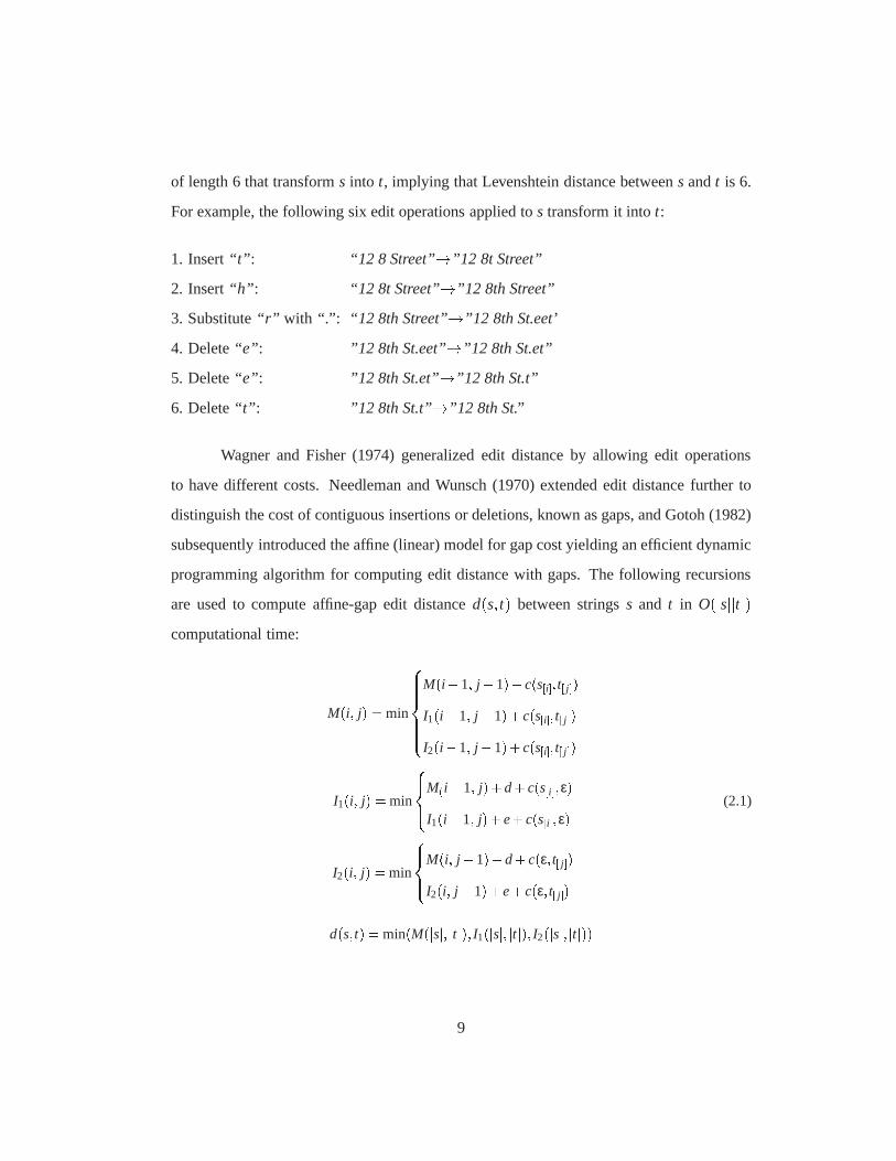
programming algorithm for computing edit distance with gaps. The following recursions
are used to compute affine-gap edit distanced(s; t) between stringss and t in O(jsjjtj)computational time:
M(i; j) = min
8>>>><>>>>:M(i �1; j �1)+c(s[i℄; t[ j ℄)I1(i �1; j �1)+c(s[i℄; t[ j ℄)I2(i �1; j �1)+c(s[i℄; t[ j ℄)
I1(i; j) = min
8><>:M(i �1; j)+d+c(s[i℄;ε)I1(i �1; j)+e+c(s[i℄;ε) (2.1)
I2(i; j) = min
8><>:M(i; j �1)+d+c(ε; t[ j ℄)I2(i; j �1)+e+c(ε; t[ j ℄)
d(s; t) = min(M(jsj; jtj); I1(jsj; jtj); I2(jsj; jtj))9
wherec(s[i℄; t[ j℄) is the cost of substituting (or matching)i-th element ofsand j-th element of
t, c(s[i℄;ε) andc(ε; t[ j℄) are the costs of inserting elementss[i℄ andt[ j℄ into the first and second
strings respectively (aligning this element with a gap in the other string), andd ande are
the costs of starting a gap and extending it by one element. Entries(i; j) in matricesM, I1,
andI2 correspond to the minimal cost of an edit operation sequencebetween string prefixes
s[1:i℄ andt[1: j℄ with the sequence respectively ending in a match/substitution, insertion into
the first string, or insertion into the second string.
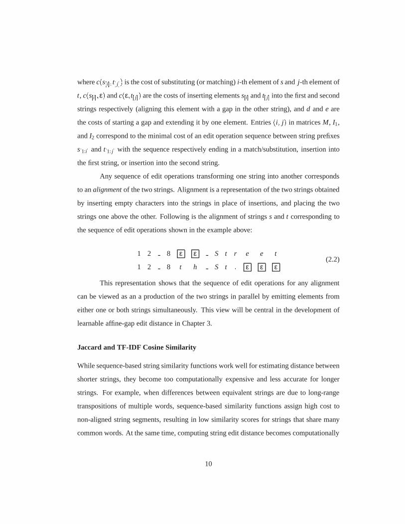
Any sequence of edit operations transforming one string into another corresponds
to analignmentof the two strings. Alignment is a representation of the two strings obtained
by inserting empty characters into the strings in place of insertions, and placing the two
strings one above the other. Following is the alignment of stringss andt corresponding to
the sequence of edit operations shown in the example above:
1 2 8 ε ε S t r e e t
1 2 8 t h S t : ε ε ε(2.2)
This representation shows that the sequence of edit operations for any alignment
can be viewed as an a production of the two strings in parallelby emitting elements from
either one or both strings simultaneously. This view will becentral in the development of
learnable affine-gap edit distance in Chapter 3.
Jaccard and TF-IDF Cosine Similarity
While sequence-based string similarity functions work well for estimating distance between
shorter strings, they become too computationally expensive and less accurate for longer
strings. For example, when differences between equivalentstrings are due to long-range
transpositions of multiple words, sequence-based similarity functions assign high cost to
non-aligned string segments, resulting in low similarity scores for strings that share many
common words. At the same time, computing string edit distance becomes computationally
10
prohibitive for larger strings such as text documents on theWeb because its computational
complexity is quadratic in string size.
The vector-space model of text avoids these problems by viewing strings as “bags
of tokens” and disregarding the order in which the tokens occur in the strings (Salton &
McGill, 1983). Jaccard similarity can then be used as the simplest method for computing
likeness as the proportion of tokens shared by both strings.If stringssandt are represented
by sets of tokensS andT , Jaccard similarity is:
simJaccard(s; t) = jS \T jjS [T j (2.3)
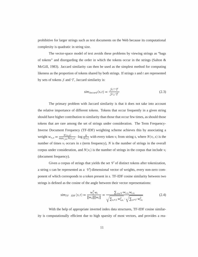
The primary problem with Jaccard similarity is that it does not take into account
the relative importance of different tokens. Tokens that occur frequently in a given string
should have higher contribution to similarity than those that occur few times, as should those
tokens that are rare among the set of strings under consideration. The Term Frequency-
Inverse Document Frequency (TF-IDF) weighting scheme achieves this by associating a
weightwvi ;s = N(vi ;s)maxvj2sN(vj ;s) � log N
N(vi ) with every tokenvi from strings, whereN(vi;s) is the
number of timesvi occurs ins (term frequency),N is the number of strings in the overall
corpus under consideration, andN(vi) is the number of strings in the corpus that includevi
(document frequency).
Given a corpus of strings that yields the setV of distinct tokens after tokenization,
a strings can be represented as ajV j-dimensional vector of weights, every non-zero com-
ponent of which corresponds to a token present ins. TF-IDF cosine similarity between two
strings is defined as the cosine of the angle between their vector representations:
simTF�IDF (s; t) = wTs wtkwskkwtk = ∑vi2V ws;vi wt;viq
∑si2S w2s;si�q∑ti2T w2
t;ti (2.4)
With the help of appropriate inverted index data structures, TF-IDF cosine similar-
ity is computationally efficient due to high sparsity of mostvectors, and provides a rea-
11
sonable off-the-shelf metric for long strings and text documents. Tokenization is typically
performed by treating each individual word of certain minimum length as a separate token,
usually excluding a fixed set of functional “stop words” and optionally stemming tokens
to their roots (Baeza-Yates & Ribeiro-Neto, 1999). An alternative tokenization scheme is
known asn-grams: it relies on using all overlapping contiguous character subsequences of
lengthn as tokens.
2.1.2 Similarity Functions for Numeric Data
Euclidean and Mahalanobis distances
For data represented by vectors in Euclidean space, the Minkowski family of metrics, also
known as theLk norms, includes most commonly used similarity measures forobjects de-
scribed byd-dimensional vectors (Duda et al., 2001):
Lk(xi ;x j) =� d
∑l=1
��xil �x jl��k�1=k
(2.5)
TheL2 norm, commonly known as Euclidean distance, is frequently used for low-
dimensional vector data. Its popularity is due to a number offactors:� Intuitive simplicity: theL2 norm corresponds to straight-line distance between points
in Euclidean space;� Invariance to rotation or translation in feature space;� Mathematical metric properties: non-negativity (L2(xi ;x j)�0)), reflexivity (L2(xi ;x j)=0 iff xi = x j ), symmetry (L2(xi ;x j) = L2(x j ;xi)), and triangle inequality (L2(xi ;x j)+L2(x j ;xk) � L2(xi ;xk)), that allow using it in many algorithms that rely on metric
assumptions.
If distance is computed among points of a given dataset, Mahalanobis distance is an
extension of Euclidean distance that takes into account thedata mean as well as variance
12
of each dimension and correlations between the different dimensions, which are estimated
from the dataset. Given a set of observation vectorsfx1; :::;xng, Mahalanobis distance is
defined as:
dMah(xi ;x j) = ((xi �x j)T�1(xi �x j))1=2 (2.6)
whereΣ�1 is the inverse of the covariance matrixΣ = 1n�1 ∑n
i=1(xi �µ)(xi �µ)T , andµ=1n ∑n
i=1 xi is the data mean.
Essentially, Mahalanobis distance attempts to give each dimension equal weight
when computing distance by scaling its contribution proportionally to variance, while tak-
ing into account co-variances between the dimensions.
Cosine Similarity
Minkowski metrics including Euclidean distance suffer from thecurse of dimensionality
when they are applied to high-dimensional data (Friedman, 1997). As the dimensionality
of the Euclidean space increases, sparsity of observationsincreases exponentially with the
number of dimensions, which leads to observations becomingequidistant in terms of Eu-
clidean distance. Cosine similarity, or normalized dot product, has been widely used as an
alternative similarity function for high-dimensional data (Duda et al., 2001):
Simcos(x;y) = xTykxkkyk = ∑di=1 xi �yiq
∑di=1 x2
i �q∑di=1y2
i
(2.7)
If applied to normalized vectors, cosine similarity obeys metric properties when
converted to distance by negating it from 1. In general, however, it is not a metric in the
mathematical sense, and it is not invariant to translationsand linear transformations.
Information-theoretic Measures
In certain domains, data can be described by probability distributions, e.g., text docu-
ments can be represented as probability distributions overwords generated by a multinomial
13
model (Pereira, Tishby, & Lee, 1993). Kullback-Leibler (KL) divergence, also known as
relative entropy, is a widely used distance measure for suchdata:
dKL(xi ;x j) = d
∑m=1
xim logxim
x jm(2.8)
wherexi andx j are instances described by probability distributions overd events:∑dm=1xim =
∑dm=1x jm = 1. Note that KL divergence is not symmetric:dKL(xi ;x j) 6= dKL(xi ;x j) for any
xi 6= x j . In domains where a symmetrical distance function is needed, Jensen-Shannon di-
vergence, also known as KL divergence to the mean, is used:
dJS(xi ;x j) = 12(dKL(xi ; xi +x j
2)+dKL(x j ; xi +x j
2)) (2.9)
Kullback-Leibler divergence is widely used in informationtheory (Cover & Thomas,
1991), where it is interpreted as the expected extra length of a message sampled from dis-
tribution xi encoded using a coding scheme that is optimal for distribution x j .
2.2 Record Linkage
As defined in Chapter 1, the goal of record linkage is identifying instances that differ syn-
tactically yet refer to the same underlying object. Matching of coreferent bibliographic
citations and identifying multiple variants of a person’s name or address in medical, cus-
tomer, or census databases are instances of this problem. A number of researchers in dif-
ferent communities have studied variants of record linkagetasks : after being introduced
in the context of matching medical records by Newcombe, Kennedy, Axford, and James
(1959), it was investigated under a number of names including merge/purge (Hernandez &
Stolfo, 1995), heterogeneous database integration (Cohen, 1998), hardening soft databases
(Cohen, Kautz, & McAllester, 2000), reference matching (McCallum, Nigam, & Ungar,
2000), de-duplication (Sarawagi & Bhamidipaty, 2002; Bhattacharya & Getoor, 2004),
fuzzy duplicate elimination (Ananthakrishna, Chaudhuri,& Ganti, 2002; Chaudhuri, Gan-
14
jam, Ganti, & Motwani, 2003), entity-name clustering and matching (Cohen & Richman,
2002), identity uncertainty (Pasula, Marthi, Milch, Russell, & Shpitser, 2003; McCallum &
Wellner, 2004a), object consolidation (Michalowski, Thakkar, & Knoblock, 2003), robust
reading (Li, Morie, & Roth, 2004), reference reconciliation (Dong, Halevy, & Madhavan,
2005), object identification (Singla & Domingos, 2005), andentity resolution (Bhattacharya
& Getoor, 2006).
The seminal work of Fellegi and Sunter (1969) described several key ideas that
have been used or re-discovered by most record linkage researchers, including combining
similarity estimates across multiple fields, using blocking to reduce the set of candidate
record pairs under consideration, and using a similarity threshold to separate the corefer-
ent and non-coreferent object pairs. Fellegi and Sunter (1969) considered record linkage
in an unsupervised setting where no examples of coreferent and non-coreferent pairs are
available. In this setting, several methods have been proposed that rely on learning prob-
abilistic models with latent variables that encode the matching decisions (Winkler, 1993;
Ravikumar & Cohen, 2004). In the past decade, a number of researchers have considered
record linkage settings where pairwise supervision is available, allowing the application of
such classification techniques as decision trees (Elfeky, Elmagarmid, & Verykios, 2002; Te-
jada, Knoblock, & Minton, 2001), logistic regression (Cohen & Richman, 2002), Bayesian
networks (Winkler, 2002), and Support Vector Machines (Bilenko & Mooney, 2003a; Co-
hen et al., 2003a; Minton, Nanjo, Knoblock, Michalowski, & Michelson, 2005) to obtain
record-level distance functions that combine the field-level similarities. These methods treat
individual field similarities as features and train a classifier to distinguish between coref-
erent and non-coreferent records, using the confidence of the classifier’s prediction as the
similarity estimate.
The majority of solutions for record linkage treat it as a modular problem that is
solved in multiple stages. In the first stage, blocking is performed to obtain a set of candidate
record pairs to be investigated for co-reference, since thecomputational cost of computing
15
pairwise similarities between all pairs of records in a large database is often prohibitive; see
Section 2.4 for discussion of blocking. In the second stage,similarity is computed between
individual fields of candidate record pairs. In the final linkage stage, similarity is computed
between candidate pairs, and highly similar records are labeled as matches that describe
the same entity. Linkage can be performed either viapairwise inference where decisions
for the different candidate pairs are made independently, or via collectiveinference over all
candidate record pairs (Pasula et al., 2003; Wellner, McCallum, Peng, & Hay, 2004; Singla
& Domingos, 2005).
2.3 Clustering
Clustering is typically defined as the problem of partitioning a dataset into disjoint groups so
that observations belonging to the same cluster are similar, while observations belonging to
different clusters are dissimilar. Clustering has been widely studied for several decades, and
a great variety of algorithms for clustering have been proposed (Jain et al., 1999). Several
large groups of clustering algorithms can be distinguishedthat include hierarchical cluster-
ing methods that attempt to create a hierarchy of data partitions (Kaufman & Rousseeuw,
1990), partitional clustering methods that separate instances into disjoint clusters (Karypis
& Kumar, 1998; Shi & Malik, 2000; Strehl, 2002; Banerjee, Merugu, Dhilon, & Ghosh,
2005b), and overlapping clustering techniques that allow instances to belong to multiple
clusters (Segal, Battle, & Koller, 2003; Banerjee, Krumpelman, Basu, Mooney, & Ghosh,
2005c).
Traditionally, clustering has been viewed as a form of unsupervised learning, since
no class labels for the data are provided. Insemi-supervised clustering, supervision from
a user is incorporated in the form of class labels or pairwiseconstraints on objects which
can be used to initialize clusters, guide the clustering process, and improve the clustering
algorithm parameters (Basu, 2005).
Work presented in Chapter 4 is based on K-Means, a widely usedclustering algo-
16
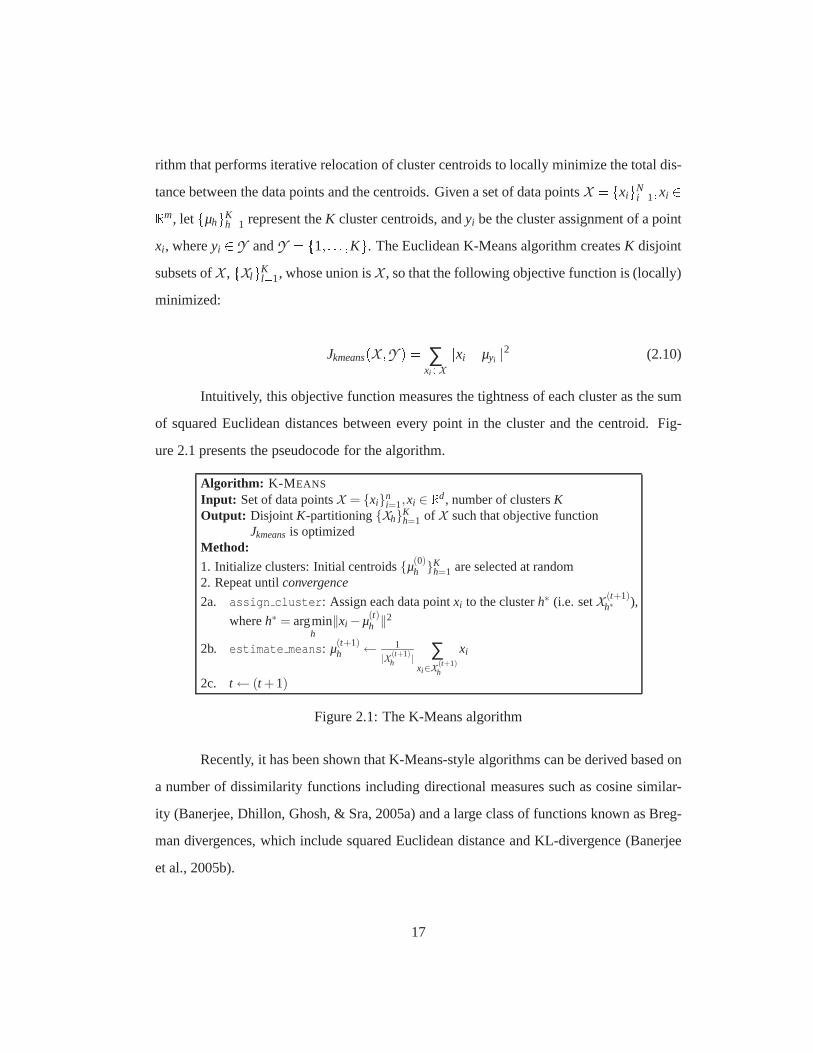
rithm that performs iterative relocation of cluster centroids to locally minimize the total dis-
tance between the data points and the centroids. Given a set of data pointsX = fxigNi=1;xi 2Rm, letfµhgK
h=1 represent theK cluster centroids, andyi be the cluster assignment of a point
xi , whereyi 2 Y andY = f1; : : : ;Kg. The Euclidean K-Means algorithm createsK disjoint
subsets ofX , fXlgKl=1, whose union isX , so that the following objective function is (locally)
minimized:
Jkmeans(X ;Y ) = ∑xi2X
kxi �µyik2 (2.10)
Intuitively, this objective function measures the tightness of each cluster as the sum
of squared Euclidean distances between every point in the cluster and the centroid. Fig-
ure 2.1 presents the pseudocode for the algorithm.
Algorithm: K-M EANS
Input: Set of data pointsX = {xi}ni=1,xi ∈ Rd, number of clustersK
Output: Disjoint K-partitioning{Xh}Kh=1 of X such that objective function
Jkmeansis optimizedMethod:
1. Initialize clusters: Initial centroids{µ(0)h }K
h=1 are selected at random2. Repeat untilconvergence
2a. assign cluster: Assign each data pointxi to the clusterh∗ (i.e. setX (t+1)h∗ ),
whereh∗ = argminh
‖xi −µ(t)h ‖2
2b. estimate means: µ(t+1)h ← 1
|X(t+1)h |
∑xi∈X
(t+1)h
xi
2c. t ← (t +1)
Figure 2.1: The K-Means algorithm
Recently, it has been shown that K-Means-style algorithms can be derived based on
a number of dissimilarity functions including directionalmeasures such as cosine similar-
ity (Banerjee, Dhillon, Ghosh, & Sra, 2005a) and a large class of functions known as Breg-
man divergences, which include squared Euclidean distanceand KL-divergence (Banerjee
et al., 2005b).
17
2.4 Blocking in Record Linkage and Clustering
Because the number of similarity computations grows quadratically with the size of the
input dataset, scaling up to large datasets is problematic for tasks that require similarities
between all instance pairs. Additionally, even for small datasets, estimation of the full
similarity matrix can be difficult if computationally costly similarity functions, distance
metrics or kernels are used. At the same time, in many tasks, the majority of similarity
computations are unnecessary because most instance pairs are highly dissimilar and have
no influence on the task output. Avoiding the unnecessary computations results in a sparse
similarity matrix, and a number of algorithms become practical for large datasets when
provided with sparse similarity matrices, e.g. the collective inference algorithms for record
linkage (Pasula et al., 2003; McCallum & Wellner, 2004b; Singla & Domingos, 2005).
Blocking methods efficiently select a subset of instance pairs for subsequent sim-
ilarity computation, ignoring the remaining pairs as highly dissimilar and therefore irrele-
vant. A number of blocking algorithms have been proposed by researchers in recent years,
all of which rely on a manually tuned set of predicates or parameters (Fellegi & Sunter,
1969; Kelley, 1985; Jaro, 1989; Hernandez & Stolfo, 1995; McCallum et al., 2000; Baxter,
Christen, & Churches, 2003; Chaudhuri et al., 2003; Jin, Li,& Mehrotra, 2003; Winkler,
2005).
Key-based blocking methods form blocks by applying some unary predicate to each
record and assigning all records that return the same value (key) to the same block (Kelley,
1985; Jaro, 1989; Winkler, 2005). For example, such predicates asSame Zipcodeor Same
3-character Prefix of Surnamecould be used to perform key-based blocking in a name-
address database, resulting in blocks that contain recordswith the same value of theZipcode
attribute and the same first three characters of theSurnameattribute, respectively.
Another popular blocking technique is the sorted neighborhood method proposed
by Hernandez and Stolfo (1995). This method forms blocks bysorting the records in a
database using lexicographic criteria and selecting all records that lie within a window of
18
fixed size. Multiple sorting passes are performed to increase coverage.
The canopies blocking algorithm of McCallum et al. (2000) relies on a similar-
ity function that allows efficient retrieval of all records within a certain distance threshold
from a randomly chosen record. Blocks are formed by randomlyselecting a “canopy cen-
ter” record and retrieving all records that are similar to the chosen record within a certain
(“loose”) threshold. Records that are closer than a “tight”threshold are removed from the
set of possible canopy centers, which is initialized with all records in the dataset. This
process is repeated iteratively, resulting in formation ofblocks selected around the canopy
centers. Inverted index-based similarity functions such as Jaccard or TF-IDF cosine sim-
ilarity are typically used with the canopies method as they allow fast selection of nearest
neighbors based on co-occurring tokens. Inverted indices are also used in the blocking
method of Chaudhuri et al. (2003), who proposed using indices based on charactern-grams
for efficient selection of candidate record pairs.
Recently, Jin et al. (2003) proposed a blocking method basedon mapping database
records to a low-dimensional metric space based on string values of individual attributes.
While this method can be used with arbitrary similarity functions, it is computationally
expensive compared to the sorting and index-based methods.
2.5 Active Learning
When training examples are selected for a learning task at random, they may be suboptimal
in the sense that they do not lead to a maximally attainable improvement in performance.
Active learningmethods attempt to identify those examples that lead to maximal accuracy
improvements when added to the training set (Lewis & Catlett, 1994; Cohn, Ghahramani,
& Jordan, 1996; Tong, 2001). During each round of active learning, the example that is
estimated to improve performance the most when added to the training set is identified and
labeled. The system is then re-trained on the training set including the newly added labeled
example.
19
Three broad classes of active learning methods exist: (1) uncertainty sampling tech-
niques (Lewis & Catlett, 1994) attempt to identify examplesfor which the learning algo-
rithm is least certain in its prediction; (2) query-by-committee methods (Seung, Opper, &
Sompolinsky, 1992) utilize a committee of learners and use disagreement between commit-
tee members as a measure of training examples’ informativeness; (3) estimation of error re-
duction techniques (Lindenbaum, Markovitch, & Rusakov, 1999; Roy & McCallum, 2001)
select examples which, when labeled, lead to greatest reduction in error by minimizing
prediction variance.
Active learning was shown to be a successful strategy for improving performance
using small amounts of training data on a number of tasks, including classification (Cohn
et al., 1996), clustering (Hofmann & Buhmann, 1998; Basu, Banerjee, & Mooney, 2004),
and record linkage (Sarawagi & Bhamidipaty, 2002; Tejada, Knoblock, & Minton, 2002).
20
Chapter 3
Learnable Similarity Functions in
Record Linkage
In this chapter, we describe the use of learnable similarityfunctions in record linkage, where
they improve the accuracy of distance estimates in two tasks: computing similarity of string
values between individual record fields, and combining suchsimilarities across multiple
fields to obtain overall record similarity. At the field level, two adaptive variants of edit
distance are described that allow learning the costs of string transformations to reflect their
relative importance in a particular domain. At the record level, we employ Support Vector
Machines, a powerful discriminative classifier, to distinguish between pairs of similar and
dissimilar records. We also propose two strategies for automatically selecting informative
pairwise training examples. These strategies do not require the human effort needed by
active learning methods, yet vastly outperform random pairselection.
3.1 Learnable Similarity Functions for Strings
In typical linkage applications, individual record fields are represented by short string val-
ues whose length does not exceed several dozen characters ortokens. For such strings,
21
differences between coreferent values frequently arise due to local string transformations at
either character or token level, e.g., misspellings, abbreviations, insertions, and deletions.
To capture such differences, similarity functions must estimate the total cost associated with
performing these transformations on string values.
As described in Section 2.1.1, edit distance estimates string dissimilarity by com-
puting the cost of a minimal sequence of edit operations required to transform one string
into another. However, the importance of different edit operations varies from domain to
domain. For example, a digit substitution makes a big difference in a street address since
it effectively changes the house or apartment number, whilea single letter substitution is
semantically insignificant because it is more likely to be caused by a typographic error or
an abbreviation. For token-level edit distance, some tokens are unimportant and therefore
their insertion cost should be low, e.g., for tokenSt. in street addresses.
Ability to vary the gap cost is a significant advantage of affine-gap edit distance over
Levenshtein edit distance, which penalizes all insertionsindependently (Bilenko & Mooney,
2002). Frequency and length of gaps in string alignments also vary from domain to domain.
For example, during linkage of coreferent bibliographic citations, gaps are common for the
authorfield where names are often abbreviated, yet rare for thetitle field which is typically
unchanged between citations to the same paper.
Therefore, adapting affine-gap edit distance to a particular domain requires learning
the costs for different edit operations and the costs of gaps. In the following subsections,
we present two methods that perform such of edit distance parameters using a corpus of
coreferent string pairs from a given domain.
3.1.1 Learnable Edit Distance with Affine Gaps
The Pair HMM Model
We propose learning the costs of edit distance parameters using a three-state pair HMM
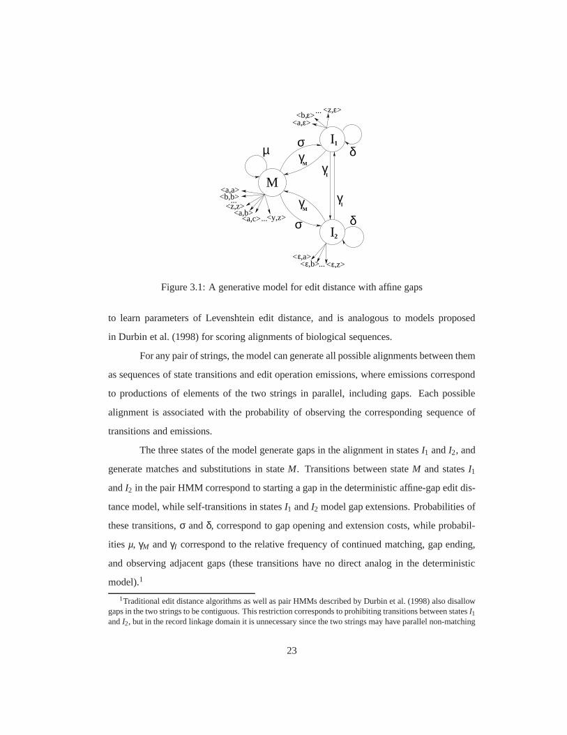
shown in Figure 3.1. It extends the one-state model used by Ristad and Yianilos (1998)
22
σ
σµ
ε<a, >ε><b,
ε><z,
I1
γM γ
I
I2
γM
<a,a><b,b>...
<a,b><a,c> <y,z>...
...
M
<z,z>γ
I
<ε...< <,b> ,z>εε
,a>
δ
δ
Figure 3.1: A generative model for edit distance with affine gaps
to learn parameters of Levenshtein edit distance, and is analogous to models proposed
in Durbin et al. (1998) for scoring alignments of biologicalsequences.
For any pair of strings, the model can generate all possible alignments between them
as sequences of state transitions and edit operation emissions, where emissions correspond
to productions of elements of the two strings in parallel, including gaps. Each possible
alignment is associated with the probability of observing the corresponding sequence of
transitions and emissions.
The three states of the model generate gaps in the alignment in statesI1 andI2, and
generate matches and substitutions in stateM. Transitions between stateM and statesI1
andI2 in the pair HMM correspond to starting a gap in the deterministic affine-gap edit dis-
tance model, while self-transitions in statesI1 andI2 model gap extensions. Probabilities of
these transitions,σ andδ, correspond to gap opening and extension costs, while probabil-
ities µ, γM andγI correspond to the relative frequency of continued matching, gap ending,
and observing adjacent gaps (these transitions have no direct analog in the deterministic
model).1
1Traditional edit distance algorithms as well as pair HMMs described by Durbin et al. (1998) also disallowgaps in the two strings to be contiguous. This restriction corresponds to prohibiting transitions between statesI1andI2, but in the record linkage domain it is unnecessary since thetwo strings may have parallel non-matching
23
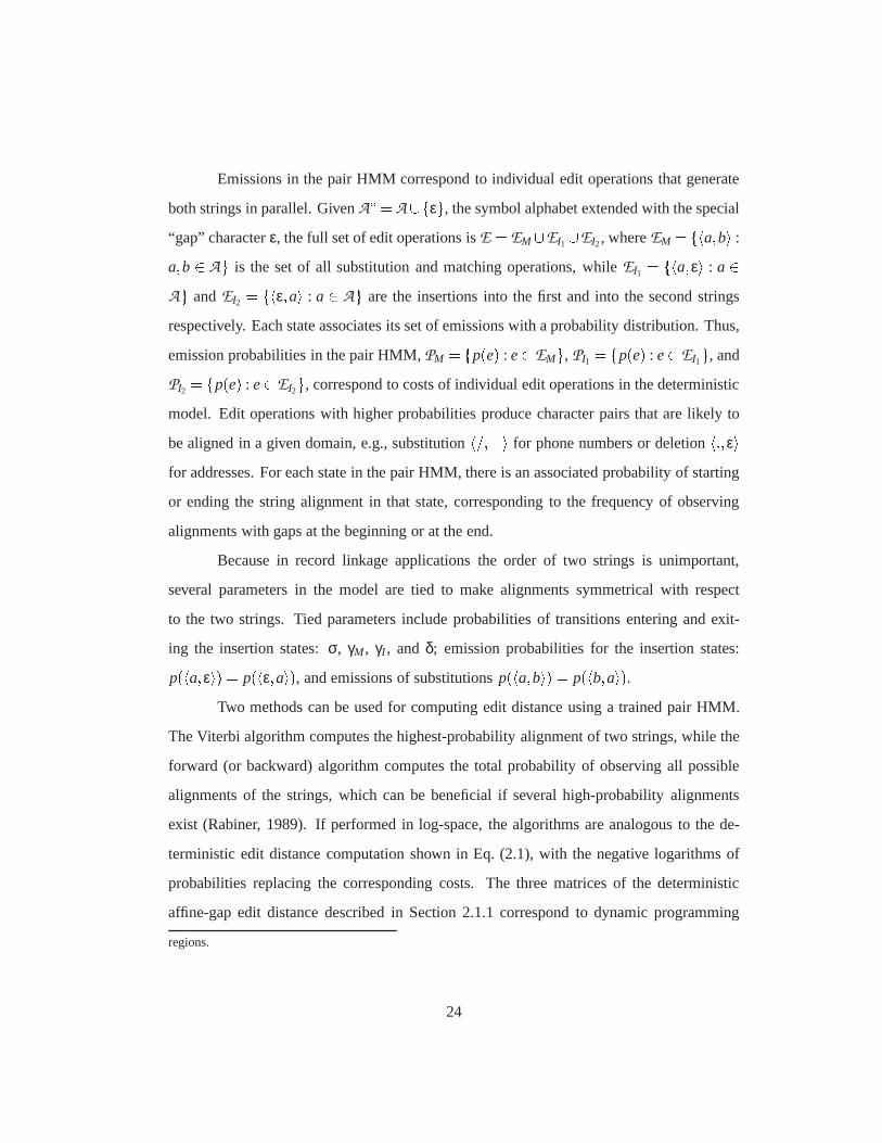
Emissions in the pair HMM correspond to individual edit operations that generate
both strings in parallel. GivenA� = A [fεg, the symbol alphabet extended with the special
“gap” characterε, the full set of edit operations isE = EM[EI1[EI2, whereEM = fha;bi :
a;b 2 Ag is the set of all substitution and matching operations, while EI1 = fha;εi : a 2Ag andEI2 = fhε;ai : a 2 Ag are the insertions into the first and into the second strings
respectively. Each state associates its set of emissions with a probability distribution. Thus,
emission probabilities in the pair HMM,PM = fp(e) : e2EMg, PI1 = fp(e) : e2EI1g, and
PI2 = fp(e) : e2EI2g, correspond to costs of individual edit operations in the deterministic
model. Edit operations with higher probabilities produce character pairs that are likely to
be aligned in a given domain, e.g., substitutionh=;�i for phone numbers or deletionh:;εifor addresses. For each state in the pair HMM, there is an associated probability of starting
or ending the string alignment in that state, correspondingto the frequency of observing
alignments with gaps at the beginning or at the end.
Because in record linkage applications the order of two strings is unimportant,
several parameters in the model are tied to make alignments symmetrical with respect
to the two strings. Tied parameters include probabilities of transitions entering and exit-
ing the insertion states:σ, γM, γI , andδ; emission probabilities for the insertion states:
p(ha;εi) = p(hε;ai), and emissions of substitutionsp(ha;bi) = p(hb;ai).Two methods can be used for computing edit distance using a trained pair HMM.
The Viterbi algorithm computes the highest-probability alignment of two strings, while the
forward (or backward) algorithm computes the total probability of observing all possible
alignments of the strings, which can be beneficial if severalhigh-probability alignments
exist (Rabiner, 1989). If performed in log-space, the algorithms are analogous to the de-
terministic edit distance computation shown in Eq. (2.1), with the negative logarithms of
probabilities replacing the corresponding costs. The three matrices of the deterministic
affine-gap edit distance described in Section 2.1.1 correspond to dynamic programming
regions.
24
matrices computed by the Viterbi, forward and backward algorithms. Each entry(i; j) in
the dynamic programming matrices for statesM, I1, andI2 contains the forward, backward,
or Viterbi probability for aligning prefixesx[1:i℄ x[1: j℄ and ending the transition sequence(s)
in the corresponding state.
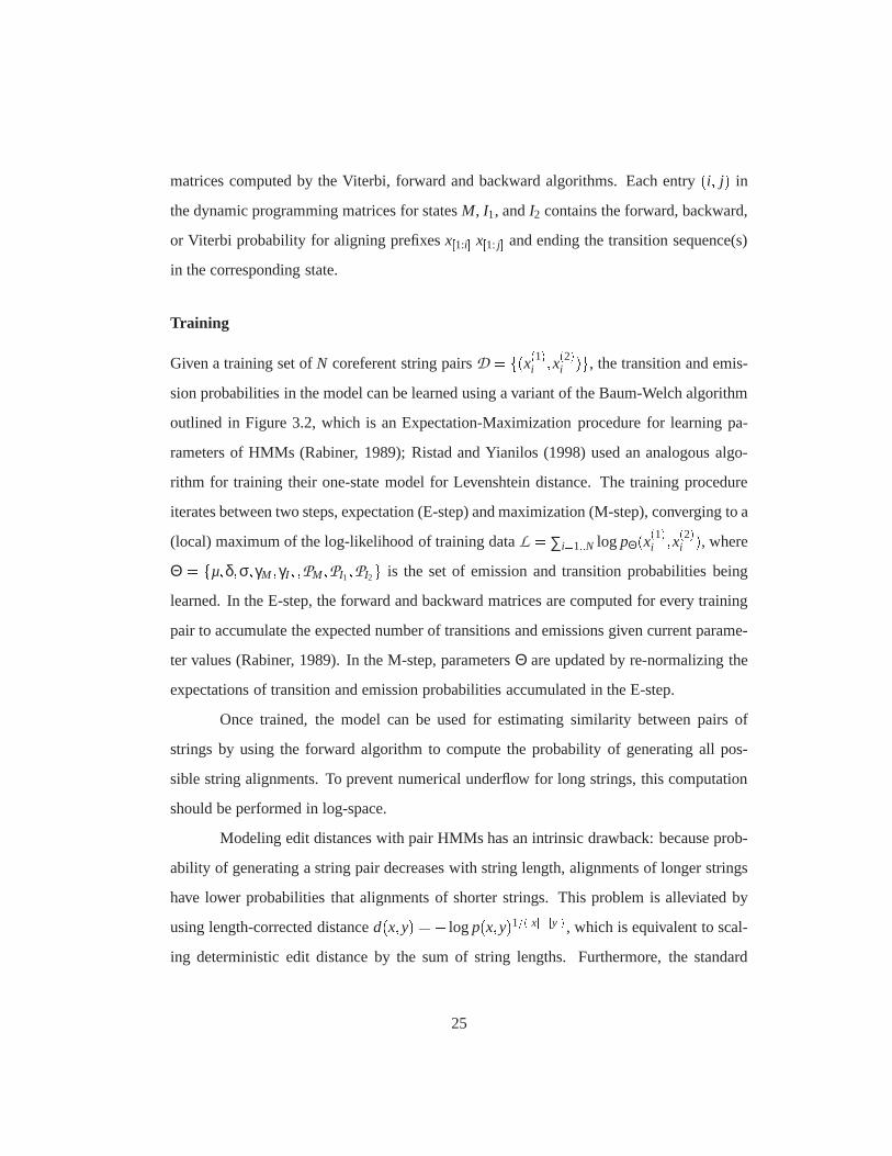
Training
Given a training set ofN coreferent string pairsD = f(x(1)i ;x(2)i )g, the transition and emis-
sion probabilities in the model can be learned using a variant of the Baum-Welch algorithm
outlined in Figure 3.2, which is an Expectation-Maximization procedure for learning pa-
rameters of HMMs (Rabiner, 1989); Ristad and Yianilos (1998) used an analogous algo-
rithm for training their one-state model for Levenshtein distance. The training procedure
iterates between two steps, expectation (E-step) and maximization (M-step), converging to a
(local) maximum of the log-likelihood of training dataL = ∑i=1::N log pΘ(x(1)i ;x(2)i ), where
Θ = fµ;δ;σ;γM ;γI ; ;PM ;PI1;PI2g is the set of emission and transition probabilities being
learned. In the E-step, the forward and backward matrices are computed for every training
pair to accumulate the expected number of transitions and emissions given current parame-
ter values (Rabiner, 1989). In the M-step, parametersΘ are updated by re-normalizing the
expectations of transition and emission probabilities accumulated in the E-step.
Once trained, the model can be used for estimating similarity between pairs of
strings by using the forward algorithm to compute the probability of generating all pos-
sible string alignments. To prevent numerical underflow forlong strings, this computation
should be performed in log-space.
Modeling edit distances with pair HMMs has an intrinsic drawback: because prob-
ability of generating a string pair decreases with string length, alignments of longer strings
have lower probabilities that alignments of shorter strings. This problem is alleviated by
using length-corrected distanced(x;y) =� logp(x;y)1=(jxj+jyj) , which is equivalent to scal-
ing deterministic edit distance by the sum of string lengths. Furthermore, the standard
25
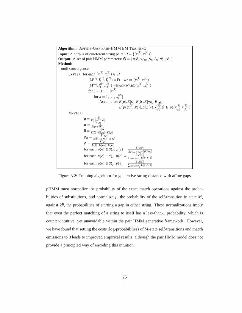
Algorithm: AFFINE-GAP PAIR-HMM EM T RAINING
Input: A corpus of coreferent string pairsD = {(x(1)i ,x(2)
i )}Output: A set of pair HMM parameters:Θ = {µ,δ,σ,γM,γI ,PM,PI1,PI2}Method:
until convergence
E-STEP: for each(x(1)i ,x(2)
i ) ∈ D
(M( f ), I ( f )1 , I ( f )
2 ) =FORWARD(x(1)i ,x(2)
i )
(M(b), I (b)1 , I (b)
2 ) =BACKWARD(x(1)i ,x(2)
i )
for j = 1, . . . , |x(1)i |
for k = 1, . . . , |x(2)i |
AccumulateE[µ],E[σ],E[δ],E[γM],E[γI ],
E[p(〈x(1)i[ j],ε〉)],E[p(〈ε,x(2)
i[k]〉)],E[p(〈x(1)
i[ j],x(2)i[k]〉)]
M-STEP:
µ= E[µ]E[µ]+2E[σ]
σ = E[σ]E[µ]+2E[σ]
δ = E[δ]E[δ]+E[γM ]+E[γI ]
γM = E[γM ]E[δ]+E[γM ]+E[γI ]
γI = E[γI ]E[δ]+E[γM ]+E[γI ]
for eachp(e) ∈ PM: p(e) = E[p(e)]∑p(eM )∈PM
E[p(eM)]
for eachp(e) ∈ PI1: p(e) = E[p(e)]∑p(eI1
)∈PI1E[p(eI1)]
for eachp(e) ∈ PI2: p(e) = E[p(e)]∑p(eI2
)∈PI2E[p(eI2)]
Figure 3.2: Training algorithm for generative string distance with affine gaps
pHMM must normalize the probability of the exact match operations against the proba-
bilities of substitutions, and normalizeµ, the probability of the self-transition in stateM,
against 2δ, the probabilities of starting a gap in either string. Thesenormalizations imply
that even the perfect matching of a string to itself has a less-than-1 probability, which is
counter-intuitive, yet unavoidable within the pair HMM generative framework. However,
we have found that setting the costs (log-probabilities) ofM-state self-transitions and match
emissions to 0 leads to improved empirical results, although the pair HMM model does not
provide a principled way of encoding this intuition.
26
Experimental Evaluation
We evaluated the proposed model for learnable affine-gap edit distance on four datasets.
Face,Constraint, Reasoning, and Reinforcementare single-field datasets containing un-
segmented citations to computer science papers in corresponding areas from theCiteseer
digital library (Giles et al., 1998).Facecontains 349 citations to 242 papers,Constraint
contains 295 citations to 199 papers, andReasoningcontains 514 citation records that rep-
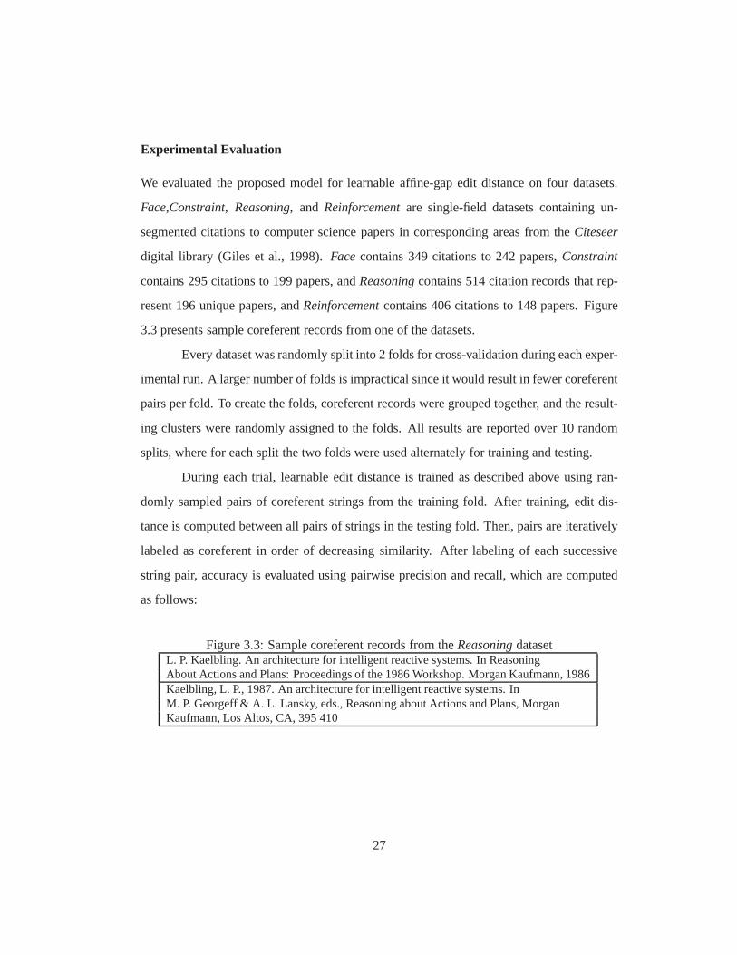
resent 196 unique papers, andReinforcementcontains 406 citations to 148 papers. Figure
3.3 presents sample coreferent records from one of the datasets.
Every dataset was randomly split into 2 folds for cross-validation during each exper-
imental run. A larger number of folds is impractical since itwould result in fewer coreferent
pairs per fold. To create the folds, coreferent records weregrouped together, and the result-
ing clusters were randomly assigned to the folds. All results are reported over 10 random
splits, where for each split the two folds were used alternately for training and testing.
During each trial, learnable edit distance is trained as described above using ran-
domly sampled pairs of coreferent strings from the trainingfold. After training, edit dis-
tance is computed between all pairs of strings in the testingfold. Then, pairs are iteratively
labeled as coreferent in order of decreasing similarity. After labeling of each successive
string pair, accuracy is evaluated using pairwise precision and recall, which are computed
as follows:
Figure 3.3: Sample coreferent records from theReasoningdatasetL. P. Kaelbling. An architecture for intelligent reactive systems. In ReasoningAbout Actions and Plans: Proceedings of the 1986 Workshop. Morgan Kaufmann, 1986Kaelbling, L. P., 1987. An architecture for intelligent reactive systems. InM. P. Georgeff & A. L. Lansky, eds., Reasoning about Actions and Plans, MorganKaufmann, Los Altos, CA, 395 410
27
precision= #o fCorrectCore f erentPairs#o f LabeledPairs
recall = #o fCorrectCore f erentPairs#o f TrueCore f erentPairs
We also compute mean average precision (MAP), defined as follows:
MAP= 1n
n
∑i=1
precision(i) (3.1)
wheren is the number of true coreferent pairs in the dataset, andprecision(i) is the pair-
wise precision computed after correctly labelingi-th coreferent pair. These measures eval-
uate how well a similarity function distinguishes between coreferent and non-coreferent
string pairs: a perfect string distance would assign highersimilarity to all coreferent pairs
than to any non-coreferent pair, achieving 1.0 on all metrics. On the precision-recall curve,
precision at any recall level corresponds to the fraction ofpairs above a certain similarity
threshold that are coreferent, while lowering the threshold results in progressive identifica-
tion of more truly coreferent pairs. For averaging the results across multiple trials, precision
is interpolated at fixed recall levels following the standard methodology from information
retrieval (Baeza-Yates & Ribeiro-Neto, 1999).
To evaluate the usefulness of adapting affine-gap string edit distance to a specific
domain, we compare the pair HMM-based learnable affine-gap edit distance with its fixed-
cost equivalent on the task of identifying equivalent field values, as well as with classic
Levenshtein distance. The following results are presented:� PHMM L EARNABLE ED: learnable affine-gap edit distance based on characters
trained as described above using the EM algorithm shown in Fig.3.2;� UNLEARNED ED: fixed-cost affine-gap edit distance (Gusfield, 1997) witha substi-
tution cost of 5, gap opening cost of 5, gap extension cost of 1, and match cost of -5,
28
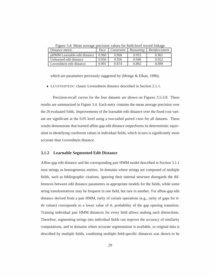
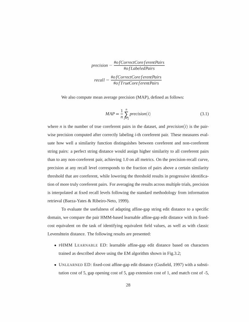
Figure 3.4: Mean average precision values for field-level record linkageDistance metric Face Constraint Reasoning Reinforcement
pHMM Learnable edit distance 0.960 0.968 0.955 0.961Unlearned edit distance 0.956 0.956 0.946 0.952Levenshtein edit distance 0.901 0.874 0.892 0.899
which are parameters previously suggested by (Monge & Elkan, 1996);� LEVENSHTEIN: classic Levenshtein distance described in Section 2.1.1.
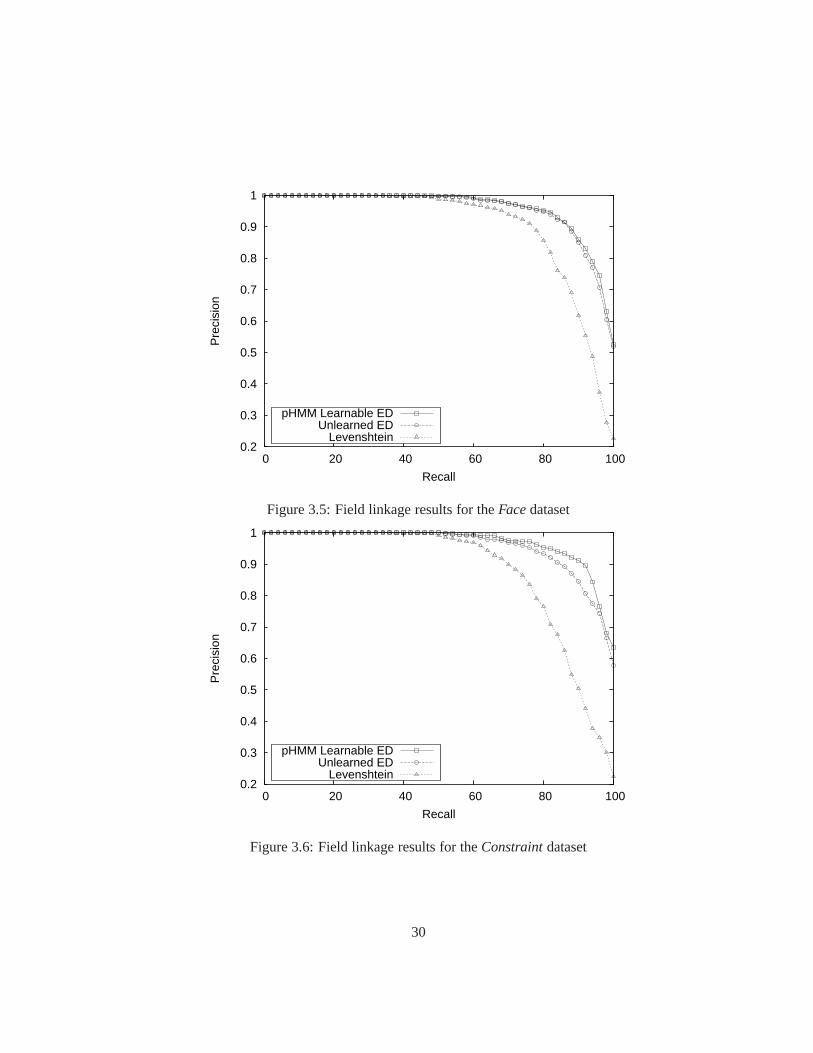
Precision-recall curves for the four datasets are shown on Figures 3.5-3.8. These
results are summarized in Figure 3.4. Each entry contains the mean average precision over
the 20 evaluated folds. Improvements of the learnable edit distance over the fixed-cost vari-
ant are significant at the 0.05 level using a two-tailed paired t-test for all datasets. These
results demonstrate that learned affine-gap edit distance outperforms its deterministic equiv-
alent in identifying coreferent values in individual fields, which in turn is significantly more
accurate than Levenshtein distance.
3.1.2 Learnable Segmented Edit Distance
Affine-gap edit distance and the corresponding pair HMM model described in Section 3.1.1
treat strings as homogeneous entities. In domains where strings are composed of multiple
fields, such as bibliographic citations, ignoring their internal structure disregards the dif-
ferences between edit distance parameters in appropriate models for the fields, while some
string transformations may be frequent in one field, but rarein another. For affine-gap edit
distance derived from a pair HMM, rarity of certain operations (e.g., rarity of gaps forti-
tle values) corresponds to a lower value ofσ, probability of the gap opening transition.
Training individual pair HMM distances for every field allows making such distinctions.
Therefore, segmenting strings into individual fields can improve the accuracy of similarity
computations, and in domains where accurate segmentation is available, or original data is
described by multiple fields, combining multiple field-specific distances was shown to be
29
0.2
0.3
0.4
0.5
0.6
0.7
0.8
0.9
1
0 20 40 60 80 100
Pre
cisi
on
Recall
pHMM Learnable EDUnlearned ED
Levenshtein
Figure 3.5: Field linkage results for theFacedataset
0.2
0.3
0.4
0.5
0.6
0.7
0.8
0.9
1
0 20 40 60 80 100
Pre
cisi
on
Recall
pHMM Learnable EDUnlearned ED
Levenshtein
Figure 3.6: Field linkage results for theConstraintdataset
30
0.1
0.2
0.3
0.4
0.5
0.6
0.7
0.8
0.9
1
0 20 40 60 80 100
Pre
cisi
on
Recall
pHMM Learnable EDUnlearned ED
Levenshtein
Figure 3.7: Field linkage results for theReasoningdataset
0.2
0.3
0.4
0.5
0.6
0.7
0.8
0.9
1
0 20 40 60 80 100
Pre
cisi
on
Recall
pHMM Learnable EDUnlearned ED
Levenshtein
Figure 3.8: Field linkage results for theReinforcementdataset
31
effective for the record linkage task, as results in Section3.2 will show.
However, in domains where supervision in the form of segmented strings for train-
ing an information extraction system is limited, field values cannot be extracted reliably.
Segmentation mistakes lead to erroneous field-level estimates of similarity, combining which
may produce worse results than utilizing a single string similarity function.
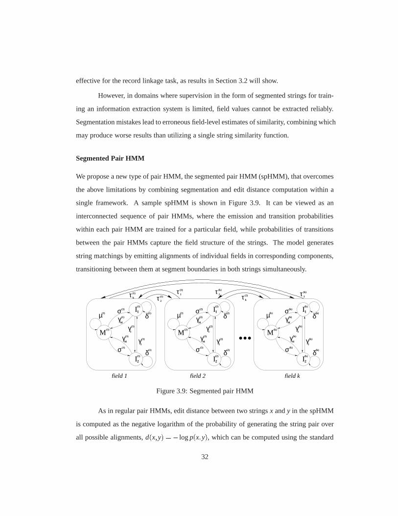
Segmented Pair HMM
We propose a new type of pair HMM, the segmented pair HMM (spHMM), that overcomes
the above limitations by combining segmentation and edit distance computation within a
single framework. A sample spHMM is shown in Figure 3.9. It can be viewed as an
interconnected sequence of pair HMMs, where the emission and transition probabilities
within each pair HMM are trained for a particular field, whileprobabilities of transitions
between the pair HMMs capture the field structure of the strings. The model generates
string matchings by emitting alignments of individual fields in corresponding components,
transitioning between them at segment boundaries in both strings simultaneously.
σµ
σ
σµ
σ
σµ
σ
field 2field 1
I1
I2
I1
γM
I2
γM
I1
γM
I2
γM
Iγ (2)
τ k
(2)(1)τ 2
...δ
δ
Iγ
γM
γM
(2)
(2)
(2)
(2)
(2)
(2)
(2)
(2)
(2)δ
δ
Iγ
Iγ
(1)
(1)
(1)
(1)
(1)
(1)
(1)(1)
(1)
(1)
(1)
δ
δ
Iγ
Iγ
(k)
(k)
(k)
(k)
(k)
(k)
(k)
(k)
(k)
(k)
(k)
M(2)
M(k)
(2)
M(1)
field k
τ ττ (k)
1
(k)
2(1)τ(2)
1k
Figure 3.9: Segmented pair HMM
As in regular pair HMMs, edit distance between two stringsx andy in the spHMM
is computed as the negative logarithm of the probability of generating the string pair over
all possible alignments,d(x;y) = � logp(x;y), which can be computed using the standard
32
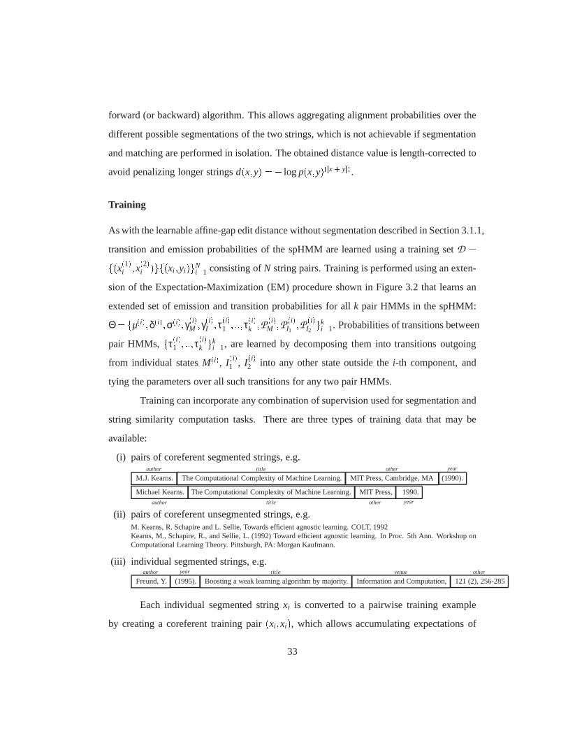
forward (or backward) algorithm. This allows aggregating alignment probabilities over the
different possible segmentations of the two strings, whichis not achievable if segmentation
and matching are performed in isolation. The obtained distance value is length-corrected to
avoid penalizing longer stringsd(x;y) =� logp(x;y)(jxj+jyj) .Training
As with the learnable affine-gap edit distance without segmentation described in Section 3.1.1,
transition and emission probabilities of the spHMM are learned using a training setD =f(x(1)i ;x(2)i )gf(xi ;yi)gNi=1 consisting ofN string pairs. Training is performed using an exten-
sion of the Expectation-Maximization (EM) procedure shownin Figure 3.2 that learns an
extended set of emission and transition probabilities for all k pair HMMs in the spHMM:
Θ= fµ(i);δ(i);σ(i);γ(i)M ;γ(i)I ;τ(i)1 ; ::;τ(i)k ;P (i)M ;P (i)
I1 ;P (i)I2 gk
i=1. Probabilities of transitions between
pair HMMs, fτ(i)1 ; ::;τ(i)k gki=1, are learned by decomposing them into transitions outgoing
from individual statesM(i), I (i)1 , I (i)2 into any other state outside thei-th component, and
tying the parameters over all such transitions for any two pair HMMs.
Training can incorporate any combination of supervision used for segmentation and
string similarity computation tasks. There are three typesof training data that may be
available:
(i) pairs of coreferent segmented strings, e.g.author
M.J. Kearns.title
The Computational Complexity of Machine Learning.other
MIT Press, Cambridge, MAyear
(1990).
Michael Kearns.author
The Computational Complexity of Machine Learning.title
MIT Press,other
1990.year
(ii) pairs of coreferent unsegmented strings, e.g.M. Kearns, R. Schapire and L. Sellie, Towards efficient agnostic learning. COLT, 1992Kearns, M., Schapire, R., and Sellie, L. (1992) Toward efficient agnostic learning. In Proc. 5th Ann. Workshop onComputational Learning Theory. Pittsburgh, PA: Morgan Kaufmann.
(iii) individual segmented strings, e.g.author
Freund, Y.year
(1995).title
Boosting a weak learning algorithm by majority.venue
Information and Computation,other
121 (2), 256-285
Each individual segmented stringxi is converted to a pairwise training example
by creating a coreferent training pair(xi ;xi), which allows accumulating expectations of
33
emissions for characters or tokens in that string along withaccumulating the expectations
of cross-component transitions. Forward and backward procedures are modified for seg-
mented string pairs so that expectations are only accumulated for component pair HMMs
that produce alignments for the corresponding fields, whilefor unsegmented string pairs,
expectations are accumulated over all component pair HMMs,thus considering alignments
over all possible segmentations of the two strings.
Because the proposed model is designed for settings where supervision is limited,
and the number of parameters in the above model can be very large, training may result
in poor parameter estimates due to sparsity of training data. To address this, we employ
a variant of shrinkage, or deleted interpolation – a smoothing technique previously used
in generative models for language modeling (Jelinek & Mercer, 1980) and information ex-
traction (Freitag & McCallum, 1999). We simultaneously train two models: one that emits
actual observations (individual characters or tokens for character-based and token-based
edit distances respectively), and another that distinguishes between several large classes of
emissions (characters, digits and punctuation for character-based edit distance, and vocab-
ulary, non-vocabulary, and numeric tokens for token-basededit distance). Parameters of
the two models are then interpolated (“shrunk”) using the method of Freitag and McCallum
(1999).
Experimental Results
We perform evaluation following the cross-validation procedure described in Section 3.1.1
on two datasets where segmentation is available:Restaurantand Cora. Restaurantis a
database obtained by Tejada et al. (2002), who integrated records from Fodor’s and Zagat’s
guidebooks to obtain 864 restaurant names and addresses that include 112 duplicates.Cora
is a collection of 1295 distinct citations to 122 Computer Science research papers from the
Cora Computer Science research paper search engine collected by McCallum et al. (2000).
The citations were automatically segmented into multiple fields such asauthor, title, venue,
34

Figure 3.10: Sample coreferent records from theCoradatasetauthor title venue year
W. W. Cohen, R. E. Shapire,and Y. Singer.
Learning to order things. In Advances in Neural Informa-tion Processing Systems 10,
1998
William W. Cohen, RobSchapire, and Yoram Singer.
Learning to order things. To appear in NIPS-97, 1997
Figure 3.11: Sample coreferent records from theRestaurantdatasetname address city phone cuisine
Fenix 8358 Sunset Blvd. West Hollywood 213/848-6677 AmericanFenix at the Argyle 8358 Sunset Blvd. W. Hollywood 213-848-6677 French(new)
etc. by an information extraction system, resulting in somenoise in the field values. Figures
3.10 and 3.11 present sample coreferent records from the twodatasets in segmented form.
SinceSPHMM is designed for domains where entities are represented by strings
containing multiple fields, we omit the available segmentation for all records in the test fold,
while retaining it in the training fold for segmented supervision of types of (i) and (iii) in the
list above. ForCora, five fields are distinguished:author, title, venue, year,andother, where
theotherfield may includes such information as page numbers, names ofeditors, location,
etc. ForRestaurant, fields name, street address, city, andcuisineare distinguished. We
employ token-based edit distance in all experiments, sincein these domains the differences
between the fields are mainly at the token, not character level.
We compare the accuracy of spHMM-learned affine-gap edit distance with the fol-
lowing baselines:� PHMM: learnable affine-gap edit distance without segmentation described in Sec-
tion 3.1.1;� SEQ: a baseline that uses labeled and unlabeled strings to train the IE system of Grenager,
Klein, and Manning [2005] that was specifically designed to handle unsupervised
data. Individual affine-gap edit distances are learned for all extracted fields, and
an SVM classifier is trained to combine them; Section 3.2 describes this process in
35
detail. During testing, the IE system segments each string into fields. Learned affine-
gap edit distances are computed for all extracted fields, andthen combined using the
SVM classifier to obtain overall string similarity estimates.
Comparison with thePHMM baseline evaluates whether incorporating segmenta-
tion in learnable affine-gap edit distance yields improvements, while comparison with the
SEQ baseline evaluates performing the segmentation and string matching steps sequen-
tially.
We consider four combinations of training data for the spHMM: segmented string
pairs only, a mixture of segmented and unsegmented pairs, a mixture of unsegmented and
individual segmented strings, and unsegmented pairs only.In all experiments 50 string pairs
are used; the three numbers in identifiersSPHMM-50-0-0, SPHMM-25-25-0, SPHMM-
0-50-50, andSPHMM-0-50-0 represent the amount of supervision for the three super-
vision types in the order listed in the previous section. Forexample,SPHMM-25-25-0
uses 25 segmented coreferent pairs, 25 unsegmented coreferent pairs, and no individual
segmented strings for training. TheSPHMM-50-0-0, SPHMM-25-25-0, andSPHMM-0-
50-0 curves demonstrate the effects of training on various combinations of segmented and
unsegmented pairwise supervision, while theSPHMM-0-50-50 curve shows the effects of
adding some individual segmented supervision to the pairwise unsegmented supervision.
Figures 3.12 and 3.13 contain precision-recall curves for the two datasets. The
results demonstrate that affine-gap edit distance based on spHMM outperforms both regular
learnable affine-gap edit distance as well as the sequentialcombination of segmentation and
learnable affine-gap edit distance on both datasets. The improvement is less pronounced on
the Cora dataset compared to theRestaurantdataset: this is due to the fact that the field
structure in citations is more complex than in restaurant records, since the ordering of the
fields varies significantly. As a result, learning an accurate segmentation model is more
difficult for Cora. If field extraction is performed in isolation, segmentation errors degrade
the quality of similarity computations significantly as canbe seen from the SEQ results.
36
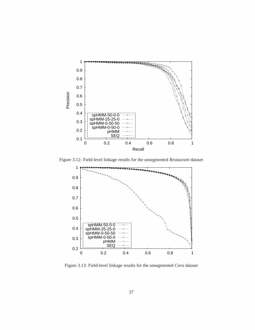
0.1
0.2
0.3
0.4
0.5
0.6
0.7
0.8
0.9
1
0 0.2 0.4 0.6 0.8 1
Pre
cisi
on
Recall
spHMM-50-0-0spHMM-25-25-0spHMM-0-50-50spHMM-0-50-0
pHMMSEQ
Figure 3.12: Field-level linkage results for the unsegmentedRestaurantdataset
0.2
0.3
0.4
0.5
0.6
0.7
0.8
0.9
1
0 0.2 0.4 0.6 0.8 1
spHMM-50-0-0spHMM-25-25-0spHMM-0-50-50spHMM-0-50-0
pHMMSEQ
Figure 3.13: Field-level linkage results for the unsegmentedCora dataset
37
In contrast,SPHMM is able to improve over non-segmented learnable edit distance by
combining similarities from the multiple alignments.
The utility of training the model on segmented versus unsegmented string pairs is
also dependent on the difficulty of the segmentation task. Because segmentations produced
by the trained model are less reliable inCora than inRestaurant, utilizing more segmented
training data does not result in statistically significant improvements. InRestaurantrecords,
the field structure is more regular, and a small amount of either segmented pairs or in-
dividual segmented strings improves results obtained withjust unsegmented pairs, as the
differences between theSPHMM-0-50-0 and the otherSPHMM results demonstrate.
Overall, the results show that incorporating segmentationinto learnable edit dis-
tance yields an improved similarity function for string linkage even without segmented
training data, while increased improvements are obtained when small amounts of seg-
mented supervision is provided.
3.2 Learnable Record Similarity
3.2.1 Combining Similarity Across Fields
Because correspondence between overall record similarityand individual field similarities
can vary greatly depending on field importance, an accurate record similarity function must
weigh fields in proportion to their contribution to the true similarity between records. For
example, similarities of theauthorandtitle fields in bibliographic citation are more signif-
icant than similarity for theyearfield, and accurate distance measure for overall citations
must reflect this. While statistical aspects of combining similarity scores for individual
fields have been addressed in previous work on record linkage(Winkler, 1999), availability
of labeled duplicates allows a more direct approach that uses a binary classifier which com-
putes a similarity function (Tejada et al., 2002; Elfeky et al., 2002; Sarawagi & Bhamidi-
paty, 2002; Cohen & Richman, 2002). Given a database containing records composed ofk
38
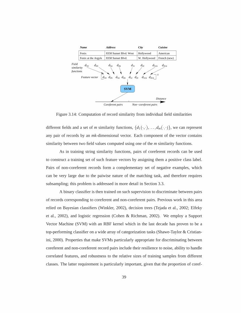
Fenix at the Argyle 8358 Sunset Blvd. W. Hollywood French (new)
8358 Sunset Blvd. WestFenix Hollywood American
Name Address City Cuisine
SVM
Distance
TFeature vector
Fieldsimilarityfunctions
Coreferent pairs Non−coreferent pairs
d2nd1n d2ad1a d1cu d2cud1c d2c
d1n d1a d1c d1cu d2cud2n d2cd2a
Figure 3.14: Computation of record similarity from individual field similarities
different fields and a set ofm similarity functions,fd1(�; �); : : : ;dm(�; �)g, we can represent
any pair of records by anmk-dimensional vector. Each component of the vector contains
similarity between two field values computed using one of them similarity functions.
As in training string similarity functions, pairs of coreferent records can be used
to construct a training set of such feature vectors by assigning them a positive class label.
Pairs of non-coreferent records form a complementary set ofnegative examples, which
can be very large due to the paiwise nature of the matching task, and therefore requires
subsampling; this problem is addressed in more detail in Section 3.3.
A binary classifier is then trained on such supervision to discriminate between pairs
of records corresponding to coreferent and non-coreferentpairs. Previous work in this area
relied on Bayesian classifiers (Winkler, 2002), decision trees (Tejada et al., 2002; Elfeky
et al., 2002), and logistic regression (Cohen & Richman, 2002). We employ a Support
Vector Machine (SVM) with an RBF kernel which in the last decade has proven to be a
top-performing classifier on a wide array of categorizationtasks (Shawe-Taylor & Cristian-
ini, 2000). Properties that make SVMs particularly appropriate for discriminating between
coreferent and non-coreferent record pairs include their resilience to noise, ability to handle
correlated features, and robustness to the relative sizes of training samples from different
classes. The latter requirement is particularly important, given that the proportion of coref-
39
erent records in a database is very difficult to estimate in realistic record linkage applications
due to the pairwise nature of the task.
Once trained, the SVM provides a confidence estimate for eachrecord pair which
can be treated as an estimate of similarity between records.The confidence estimate is de-
rived from themarginof a particular example, that is, its distance from the hyperplane that
separates the two classes. It has been shown that margins canbe converted to confidence or
probability values via a logistic transformation (Wahba, 1999; Platt, 1999b).
Figure 3.14 illustrates the process of computing record similarity using multiple
similarity measures over each field and an SVM to categorize the resulting feature vector
as belonging to the class of duplicates or non-duplicates. For each field of the database,
two similarity functions,d1 andd2, are applied to compute similarity for that field. The
values computed by these measures form the feature vector that is then classified by a
support vector machine, producing a confidence value that represents similarity between
the database records.
The Overall Record Linkage Framework
An overall view of our system, MARLIN (Multiply Adaptive Record Linkage with INduc-
tion), is presented in Figure 3.15. The training phase consists of two steps. First, the
learnable string similarity functions are trained for eachrecord field. The training corpus of
field-level coreferent and non-coreferent pairs is obtained by taking pairs of values for each
field from the set of coreferent record pairs. Because equivalent records may contain indi-
vidual fields that are not coreferent, training data can be noisy. For example, if one record
describing a restaurant contains“Asian” in thecuisinefield, and an equivalent record con-
tains “Seafood”, a noisy training pair is formed that implies equivalence between these
two strings. However, this issue does not pose a serious problem for our approach for two
reasons. First, particularly noisy fields that are unhelpful for identifying record-level dupli-
cates will be considered irrelevant by the classifier that combines similarities from different
40
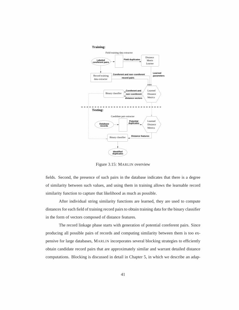
Distance
LearnerMetric
Learned parametersRecord training
data extractor
Databaserecords
duplicatesPotential
DistanceLearned
Metrics
Binary classifier
DistanceMetrics
LearnedBinary classifier
Training:
Field training data extractor
Field duplicates
Distance features
Identifiedduplicates
Labeledcoreferent pairs
Coreferent and non−coreferent
record pairs
Coreferent and
non−coreferent
distance vectors
Candidate pair extractor
Testing:
Figure 3.15: MARLIN overview
fields. Second, the presence of such pairs in the database indicates that there is a degree
of similarity between such values, and using them in training allows the learnable record
similarity function to capture that likelihood as much as possible.
After individual string similarity functions are learned,they are used to compute
distances for each field of training record pairs to obtain training data for the binary classifier
in the form of vectors composed of distance features.
The record linkage phase starts with generation of potential coreferent pairs. Since
producing all possible pairs of records and computing similarity between them is too ex-
pensive for large databases, MARLIN incorporates several blocking strategies to efficiently
obtain candidate record pairs that are approximately similar and warrant detailed distance
computations. Blocking is discussed in detail in Chapter 5,in which we describe an adap-
41
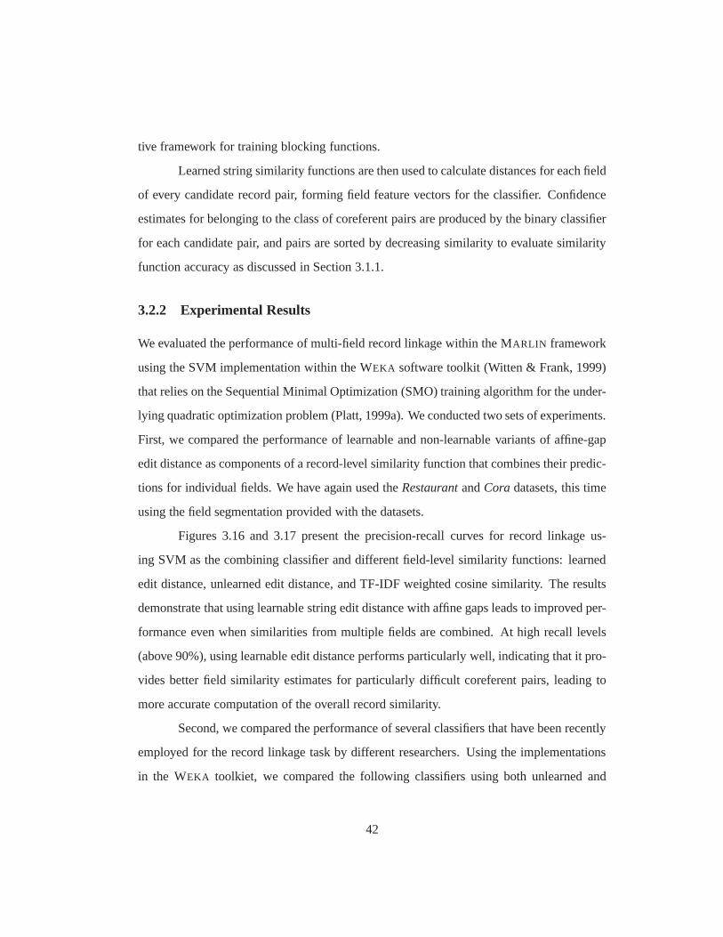
tive framework for training blocking functions.
Learned string similarity functions are then used to calculate distances for each field
of every candidate record pair, forming field feature vectors for the classifier. Confidence
estimates for belonging to the class of coreferent pairs areproduced by the binary classifier
for each candidate pair, and pairs are sorted by decreasing similarity to evaluate similarity
function accuracy as discussed in Section 3.1.1.
3.2.2 Experimental Results
We evaluated the performance of multi-field record linkage within the MARLIN framework
using the SVM implementation within the WEKA software toolkit (Witten & Frank, 1999)
that relies on the Sequential Minimal Optimization (SMO) training algorithm for the under-
lying quadratic optimization problem (Platt, 1999a). We conducted two sets of experiments.
First, we compared the performance of learnable and non-learnable variants of affine-gap
edit distance as components of a record-level similarity function that combines their predic-
tions for individual fields. We have again used theRestaurantandCora datasets, this time
using the field segmentation provided with the datasets.
Figures 3.16 and 3.17 present the precision-recall curves for record linkage us-
ing SVM as the combining classifier and different field-levelsimilarity functions: learned
edit distance, unlearned edit distance, and TF-IDF weighted cosine similarity. The results
demonstrate that using learnable string edit distance withaffine gaps leads to improved per-
formance even when similarities from multiple fields are combined. At high recall levels
(above 90%), using learnable edit distance performs particularly well, indicating that it pro-
vides better field similarity estimates for particularly difficult coreferent pairs, leading to
more accurate computation of the overall record similarity.
Second, we compared the performance of several classifiers that have been recently
employed for the record linkage task by different researchers. Using the implementations
in the WEKA toolkiet, we compared the following classifiers using both unlearned and
42
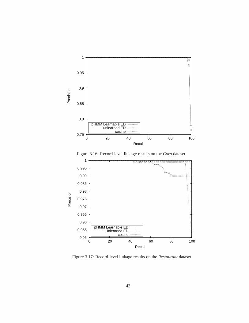
0.75
0.8
0.85
0.9
0.95
1
0 20 40 60 80 100
Pre
cisi
on
Recall
pHMM Learnable EDunlearned ED
cosine
Figure 3.16: Record-level linkage results on theCora dataset
0.95
0.955
0.96
0.965
0.97
0.975
0.98
0.985
0.99
0.995
1
0 20 40 60 80 100
Pre
cisi
on
Recall
pHMM Learnable EDUnlearned ED
cosine
Figure 3.17: Record-level linkage results on theRestaurantdataset
43
learnable affine-gap edit distances as the underlying field similarity functions:� SVM-RBF: Support Vector Machine with the Gaussian kernel;� SVM-LINEAR : Support Vector Machine with the linear kernel;� ADABOOST: boosting algorithm of Freund and Schapire (1996) that usesJ48, WEKA ’s
implementation of C4.5 decision tree as the base classifier (Quinlan, 1993);� MAX ENT: logistic regression (le Cessie & van Houwelingen, 1992);� BAYESNET: a Bayesian Network learner that uses the K2 structure learning algo-
rithm (Cooper & Herskovits, 1992).
Figures 3.19 and 3.20 present results for the experiments that used learnable affine-
gap edit distance onRestaurantandCora datasets, while mean average precision (MAP)
values for all experiments are shown in Figure 3.18.
Overall, the results demonstrate that Support Vector Machines yield the best accu-
racy on both datasets, outperforming the other classifiers significantly. Both the Gaussian
and the linear kernel provide equivalently good performance, which is not surprising since
the classification is performed on a very low-dimensional problem. Other classifiers per-
form significantly worse for both datasets. We conclude thatSVM-based learnable record
similarity is a robust, accurate similarity function for combining similarities of multiple
fields in the record linkage setting. We also note that using learnable affine-gap edit distance
as the field similarity function provides better results than using unlearned edit distance, al-
though statistically significant differences are only observed on parts of the learning curve
for most classifiers (e.g., for SVM-RBF and SVM-LINEAR the improvements are statisti-
cally significant at 0.05 level using a two-tailed paired t-test only at 98% and 100% recall
respectively). However, the improvements are consistent and suggest that using learnable
edit distance for field-level comparisons leads to accuracyimprovements even when fields
are combined by a classifier.
44

Figure 3.18: Mean average precision values for record-level linkageRestaurant Cora
pHMM ED Unlearned ED pHMM ED Unlearned EDSVM-RBF 0.999 0.996 0.998 0.997SVM-LINEAR 0.994 0.994 0.998 0.997ADABOOST 0.948 0.927 0.975 0.974MAX ENT 0.938 0.937 0.824 0.815BAYESNET 0.884 0.873 0.976 0.967
3.3 Training-Set Construction for Learning Similarity Fun ctions
Training string and record similarity functions in real-world scenarios requires selecting
a set of pairs for a human expert to label as coreferent or non-coreferent, or asking the
expert to identify all groups of coreferent records in the dataset, which is not feasible for
large datasets. Since typical corpora and databases contain few coreferent records, selecting
random pairs as potential training examples leads to training sets with extremely few coref-
erent pairs (positive examples). As a result, such randomlyselected training sets are highly
skewed toward non-coreferent pairs, which leads to suboptimal performance of similarity
functions trained on this data. We propose two heuristic approaches for collecting training
data: static-active learning and weakly-labeled selection, and present experimental results
on their effectiveness.
3.3.1 Likely-positive Selection of Training Pairs
Traditional active learning systems are “dynamic”: labelsof training examples selected in
earlier rounds influence which unlabeled examples are deemed most informative in sub-
sequent rounds. While prior work has examined dynamic active learning approaches to
adaptive record linkage (Sarawagi & Bhamidipaty, 2002; Tejada et al., 2002), such strate-
gies may not always be feasible due to high computational costs exacerbated by the large
number of potential training examples. We propose using a “static” active learning method
for selecting pairs of records that arelikely to be coreferent, as a middle ground between
45
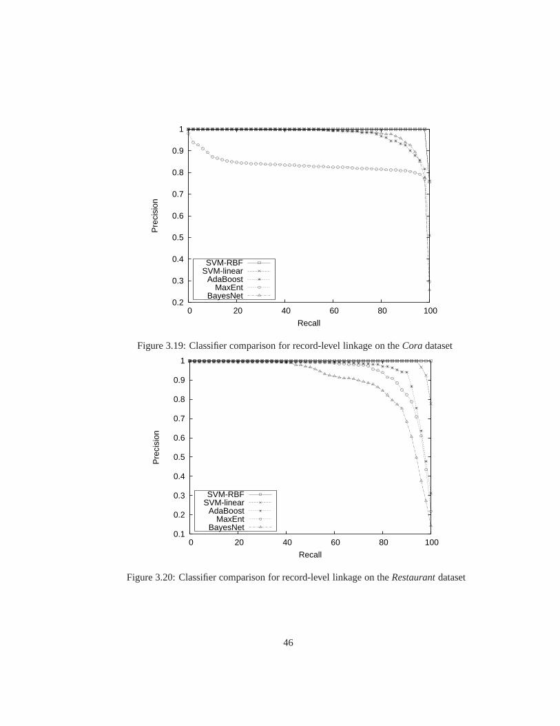
0.2
0.3
0.4
0.5
0.6
0.7
0.8
0.9
1
0 20 40 60 80 100
Pre
cisi
on
Recall
SVM-RBFSVM-linear
AdaBoostMaxEnt
BayesNet
Figure 3.19: Classifier comparison for record-level linkage on theCoradataset
0.1
0.2
0.3
0.4
0.5
0.6
0.7
0.8
0.9
1
0 20 40 60 80 100
Pre
cisi
on
Recall
SVM-RBFSVM-linear
AdaBoostMaxEnt
BayesNet
Figure 3.20: Classifier comparison for record-level linkage on theRestaurantdataset
46
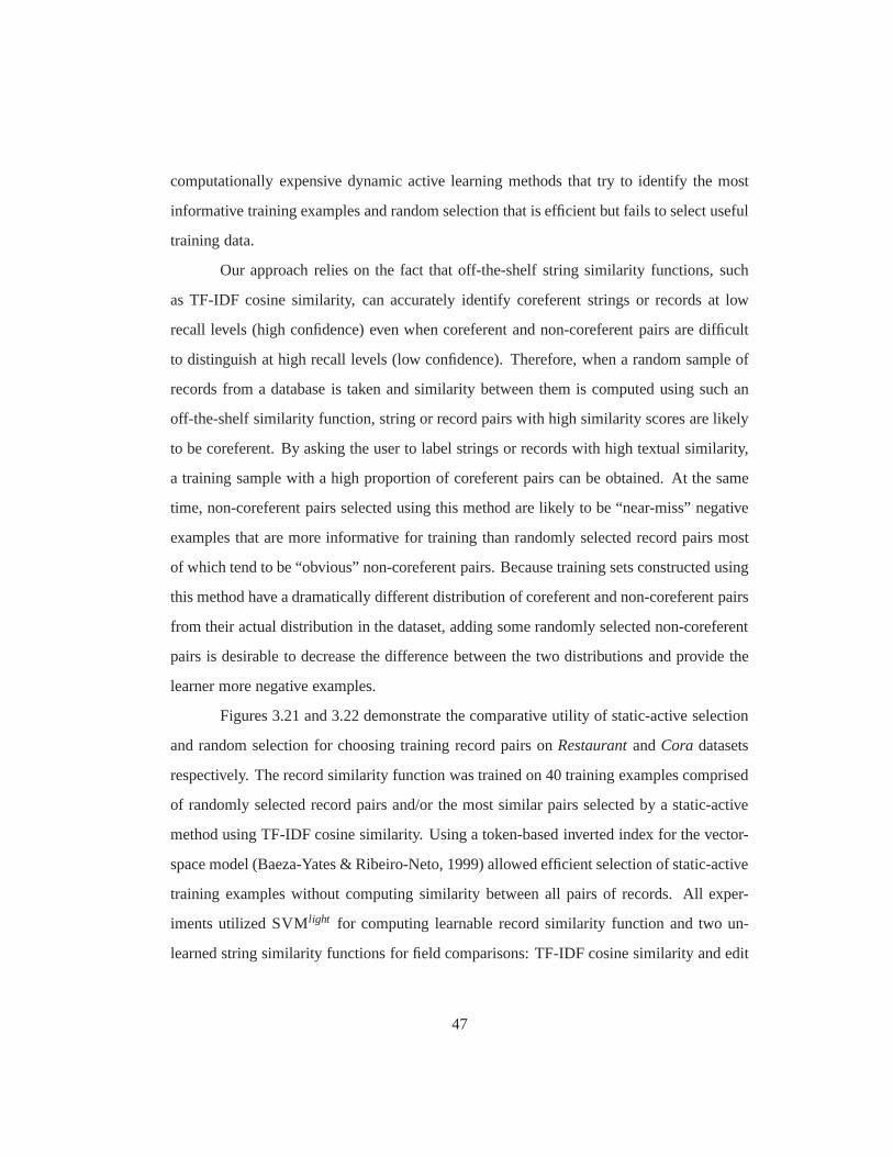
computationally expensive dynamic active learning methods that try to identify the most
informative training examples and random selection that isefficient but fails to select useful
training data.
Our approach relies on the fact that off-the-shelf string similarity functions, such
as TF-IDF cosine similarity, can accurately identify coreferent strings or records at low
recall levels (high confidence) even when coreferent and non-coreferent pairs are difficult
to distinguish at high recall levels (low confidence). Therefore, when a random sample of
records from a database is taken and similarity between themis computed using such an
off-the-shelf similarity function, string or record pairswith high similarity scores are likely
to be coreferent. By asking the user to label strings or records with high textual similarity,
a training sample with a high proportion of coreferent pairscan be obtained. At the same
time, non-coreferent pairs selected using this method are likely to be “near-miss” negative
examples that are more informative for training than randomly selected record pairs most
of which tend to be “obvious” non-coreferent pairs. Becausetraining sets constructed using
this method have a dramatically different distribution of coreferent and non-coreferent pairs
from their actual distribution in the dataset, adding some randomly selected non-coreferent
pairs is desirable to decrease the difference between the two distributions and provide the
learner more negative examples.
Figures 3.21 and 3.22 demonstrate the comparative utility of static-active selection
and random selection for choosing training record pairs onRestaurantandCora datasets
respectively. The record similarity function was trained on 40 training examples comprised
of randomly selected record pairs and/or the most similar pairs selected by a static-active
method using TF-IDF cosine similarity. Using a token-basedinverted index for the vector-
space model (Baeza-Yates & Ribeiro-Neto, 1999) allowed efficient selection of static-active
training examples without computing similarity between all pairs of records. All exper-
iments utilized SVMlight for computing learnable record similarity function and twoun-
learned string similarity functions for field comparisons:TF-IDF cosine similarity and edit
47
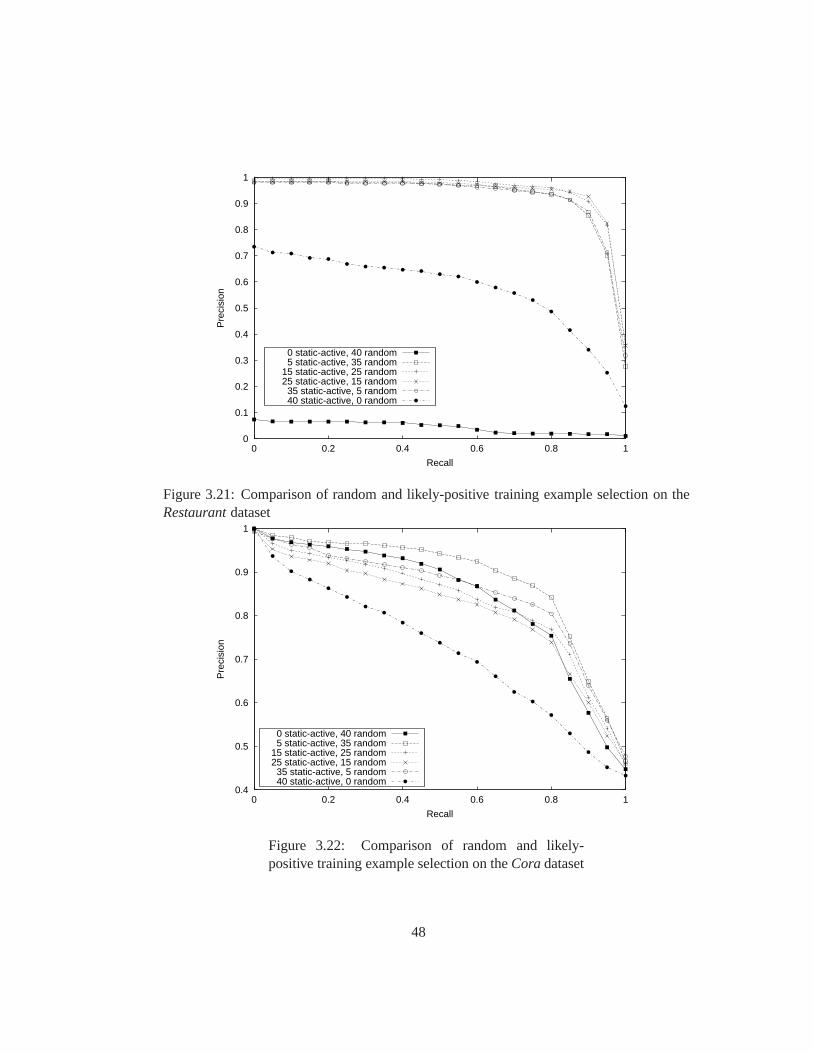
0
0.1
0.2
0.3
0.4
0.5
0.6
0.7
0.8
0.9
1
0 0.2 0.4 0.6 0.8 1
Pre
cisi
on
Recall
0 static-active, 40 random5 static-active, 35 random
15 static-active, 25 random25 static-active, 15 random
35 static-active, 5 random40 static-active, 0 random
Figure 3.21: Comparison of random and likely-positive training example selection on theRestaurantdataset
0.4
0.5
0.6
0.7
0.8
0.9
1
0 0.2 0.4 0.6 0.8 1
Pre
cisi
on
Recall
0 static-active, 40 random5 static-active, 35 random
15 static-active, 25 random25 static-active, 15 random35 static-active, 5 random40 static-active, 0 random
Figure 3.22: Comparison of random and likely-positive training example selection on theCoradataset
48
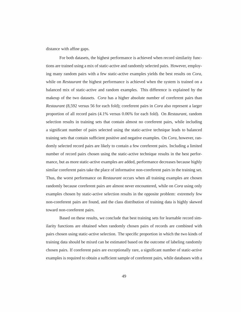
distance with affine gaps.
For both datasets, the highest performance is achieved whenrecord similarity func-
tions are trained using a mix of static-active and randomly selected pairs. However, employ-
ing many random pairs with a few static-active examples yields the best results onCora,
while on Restaurantthe highest performance is achieved when the system is trained on a
balanced mix of static-active and random examples. This difference is explained by the
makeup of the two datasets.Cora has a higher absolute number of coreferent pairs than
Restaurant(8,592 versus 56 for each fold); coreferent pairs inCora also represent a larger
proportion of all record pairs (4.1% versus 0.06% for each fold). On Restaurant, random
selection results in training sets that contain almost no coreferent pairs, while including
a significant number of pairs selected using the static-active technique leads to balanced
training sets that contain sufficient positive and negativeexamples. OnCora, however, ran-
domly selected record pairs are likely to contain a few coreferent pairs. Including a limited
number of record pairs chosen using the static-active technique results in the best perfor-
mance, but as more static-active examples are added, performance decreases because highly
similar coreferent pairs take the place of informative non-coreferent pairs in the training set.
Thus, the worst performance onRestaurantoccurs when all training examples are chosen
randomly because coreferent pairs are almost never encountered, while onCorausing only
examples chosen by static-active selection results in the opposite problem: extremely few
non-coreferent pairs are found, and the class distributionof training data is highly skewed
toward non-coreferent pairs.
Based on these results, we conclude that best training sets for learnable record sim-
ilarity functions are obtained when randomly chosen pairs of records are combined with
pairs chosen using static-active selection. The specific proportion in which the two kinds of
training data should be mixed can be estimated based on the outcome of labeling randomly
chosen pairs. If coreferent pairs are exceptionally rare, asignificant number of static-active
examples is required to obtain a sufficient sample of coreferent pairs, while databases with a
49
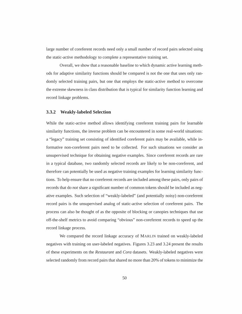
large number of coreferent records need only a small number of record pairs selected using
the static-active methodology to complete a representative training set.
Overall, we show that a reasonable baseline to which dynamicactive learning meth-
ods for adaptive similarity functions should be compared isnot the one that uses only ran-
domly selected training pairs, but one that employs the static-active method to overcome
the extreme skewness in class distribution that is typical for similarity function learning and
record linkage problems.
3.3.2 Weakly-labeled Selection
While the static-active method allows identifying coreferent training pairs for learnable
similarity functions, the inverse problem can be encountered in some real-world situations:
a “legacy” training set consisting of identified coreferentpairs may be available, while in-
formative non-coreferent pairs need to be collected. For such situations we consider an
unsupervised technique for obtaining negative examples. Since coreferent records are rare
in a typical database, two randomly selected records are likely to be non-coreferent, and
therefore can potentially be used as negative training examples for learning similarity func-
tions. To help ensure that no coreferent records are included among these pairs, only pairs of
records that donotshare a significant number of common tokens should be included as neg-
ative examples. Such selection of “weakly-labeled” (and potentially noisy) non-coreferent
record pairs is the unsupervised analog of static-active selection of coreferent pairs. The
process can also be thought of as the opposite of blocking or canopies techniques that use
off-the-shelf metrics to avoid comparing “obvious” non-coreferent records to speed up the
record linkage process.
We compared the record linkage accuracy of MARLIN trained on weakly-labeled
negatives with training on user-labeled negatives. Figures 3.23 and 3.24 present the results
of these experiments on theRestaurantandCora datasets. Weakly-labeled negatives were
selected randomly from record pairs that shared no more than20% of tokens to minimize the
50
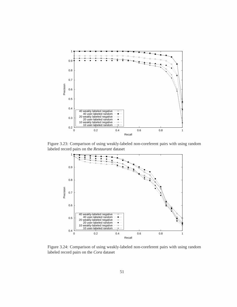
0.2
0.3
0.4
0.5
0.6
0.7
0.8
0.9
1
0 0.2 0.4 0.6 0.8 1
Pre
cisi
on
Recall
40 weakly labeled negative40 user-labeled random
20 weakly labeled negative20 user-labeled random
10 weakly labeled negative10 user-labeled random
Figure 3.23: Comparison of using weakly-labeled non-coreferent pairs with using randomlabeled record pairs on theRestaurantdataset
0.4
0.5
0.6
0.7
0.8
0.9
1
0 0.2 0.4 0.6 0.8 1
Pre
cisi
on
Recall
40 weakly-labeled negative40 user-labeled random
20 weakly-labeled negative20 user-labeled random
10 weakly-labeled negative10 user-labeled random
Figure 3.24: Comparison of using weakly-labeled non-coreferent pairs with using randomlabeled record pairs on theCoradataset
51
noise. All experiments used training sets composed of two parts: half the examples were
positives randomly selected among user-labeled coreferent pairs, and the other half was
composed of either weakly-labeled non-coreferent recordsor randomly selected labeled
record pairs. SVMlight was employed to compute record similarity, and TF-IDF cosine
similarity and edit distance with affine gaps were used as theunderlying string similarity
functions for individual fields.
The results again demonstrate that the utility of the heuristic selection of training
data for similarity function learning is dataset-dependent. OnRestaurant, where coreferent
pairs are scarce and randomly selected records are truely non-coreferent with very high
probability, using weakly-labeled non-coreferent pairs yields results identical to randomly
selected labeled coreferent pairs when a large number of examples is selected, and improves
slightly over random selection when the training set is small. We conjecture that biasing
the SVM with “negative but slightly similar” examples when very little training data is
available allows learning a better separating hyperplane.On Cora, using weakly-labeled
negatives leads to slight degradation of system accuracy, which is expected since coreferent
pairs are relatively frequent, and noise is likely to be introduced when negative examples
are collected in an unsupervised manner. However, the drop in performance is small, and in
situations where human labeling of negatives is expensive or infeasible (e.g. due to privacy
issues), using weakly-labeled selection is a viable avenuefor unsupervised acquisition of
negative training examples for similarity function learning.
3.4 Related Work
Several researchers described methods for learning stringsimilarity functions in prior work.
For string edit distance, Ristad and Yianilos (1998) proposed learning the costs of individual
edit operations of Levenshtein distance using a probabilistic generative model. In their
model, a string alignment is equivalent to a sequence of character pairs generated by edit
operations emitted by a hidden Markov model with a single non-terminal state. We have
52
followed the same approach in developing a learning model for affine-gap edit distance,
which provides significantly better similarity estimates for natural text strings (Bilenko &
Mooney, 2002; Cohen et al., 2003a).
Both our model and the model of Ristad-Yianilos are instances of pair Hidden
Markov Models, proposed earlier for biological sequence alignments in bioinformatics (Durbin
et al., 1998). Using such models for record linkage requiresseveral modifications that we
have described. Among those, parameter tying, gap-to-gap transitions, and length normal-
ization are important for obtaining good performance of pair HMM-based edit distance in
natural language string similarity computations.
Two other models for learning the costs of individual edit operations have been
proposed by Zhu and Ungar (2000) and Yancey (2004). Zhu and Ungar (2000) have used
genetic algorithms for learning the costs of several manually constructed edit operations.
Yancey (2004) has employed a variant of Expectation-Maximization for learning the prob-
abilities of individual edit operations, where only highest-probability (Viterbi) alignments
were used to accumulate expectations. Both of these approaches are adaptive variants of
Levenshtein distance and do not include taking gaps into account.
In recent years, two models of learnable edit distance have been proposed based
on discriminative classifiers. Joachims (2003) formulatedthe problem of learning edit op-
eration costs as maximum-margin optimization, and showed how it can be solved using
SVMs. However, this formulation relies on availability of actual string alignments, not just
coreferent string pairs, and therefore requires significant labeling effort to obtain training
data. McCallum, Bellare, and Pereira (2005) described a model for learning the parameters
of affine-gap edit distance based on Conditional Random Fields (CRFs), a discriminative
analog of HMMs. While they have obtained improvements over the field-level results we
presented in Section 3.1.1 on some of the datasets, their method relies on a number of extra
matching features, some of which could also be implemented in the HMM-based model.
Additionally, training algorithms for CRF-based models are more complex than EM-based
53
training of HMMs and incur significant computational costs.
A number of record linkage researchers have relied on classifiers to combine simi-
larity estimates across multiple fields. Approaches in the statistical literature has tradition-
ally relied on generative classifiers such as Naive Bayes andBayesian networks (Winkler,
2002), while in recent machine learning research a number ofclassifiers have been used,
including decision trees (Elfeky et al., 2002; Tejada et al., 2002; Sarawagi & Bhamidipaty,
2002) and logistic regression (Cohen & Richman, 2002). We have shown that Support Vec-
tor Machines outperform these methods significantly on bothdatasets that we considered.
Sarawagi and Bhamidipaty (2002) and Tejada et al. (2002) have proposed active
learning methods that obtain informative training examples for learning record-level sim-
ilarity functions between records. The training set construction strategies we described in
Section 3.3 approximate these methods without the computational cost of active learning
for selecting likely positives, and without the need for a human oracle for weak negatives.
Recent work on record linkage has focused on the third stage of the record link-
age process described in Section 2.2: clustering for obtaining groups of coreferent records.
In particular, a number of methods have been proposed forcollectivegrouping coreferent
records and obtaining the complete partitioning of datasets into such groups (Pasula et al.,
2003; Wellner et al., 2004; Li et al., 2004; Singla & Domingos, 2005). Our work addresses
an orthogonal problem, accurate computation of record and field similarities, and the meth-
ods presented in this chapter can be used as input to the collective linkage approaches, since
they rely on pairwise similarity estimates between recordsor their fields.
3.5 Chapter Summary
In this chapter, we have shown how learnable similarity functions lead to significant perfor-
mance improvements in the record linkage task. Because record linkage requires accurate
distance estimates between individual field values and overall records, adapting similarity
functions that provide these estimates allows learning domain-specific parameters to com-
54

pute similarity with higher accuracy.
Two learnable variants of affine-gap edit distance based on pair HMMs that we
described learn edit operation and gap costs that discriminate between coreferent and non-
coreferent strings. For record-level similarity, we have shown that using Support Vector
Machines leads to accurate distance estimations between records composed of multiple
fields. We have demonstrated that employing learnable field-level similarity functions is
still advantageous over using unlearned methods in multi-field domains when field similar-
ities are combined by a classifier. Finally, we have shown that informative training examples
for these methods can be collected without relying on activelearning methods, and possibly
without even relying on human supervision.
55
Chapter 4
Learnable Similarity Functions in
Semi-supervised Clustering
In this chapter, we show how learnable similarity functionsimprove clustering accuracy
when employed in a semi-supervised clustering setting. We describe a probabilistic model
for semi-supervised clustering based on Hidden Markov Random Fields (HMRFs) that ac-
commodates a wide variety of learnable similarity functions. This model yields a clustering
algorithm, HMRF-KMEANS, that integrates similarity function learning with constraint-
based clustering, improving on algorithms that perform these tasks in isolation.
4.1 Similarity Functions in Clustering
As discussed in Section 2.3, clustering inherently relies on similarity estimations as its goal
is to group instances that are alike while separating instances that are dissimilar. For many
datasets, off-the-shelf functions may fail in providing similarity estimates that place same-
cluster points nearby and different-cluster points far apart, preventing the discovery of a
desired partitioning of a dataset. Examples of same-cluster and different-cluster instance
pairs that are available in the semi-supervised clusteringsetting provide supervision for
56
training the similarity function to produce appropriate distance estimates, making it easier
to create clusters that respect the pairwise supervision when grouping the unlabeled data.
For some datasets, clusters of different shapes may be desirable, which effectively
indicates that datapoints in these clusters lie in different subspaces of the overall data
space. Recovering such partitioning requires using an individual similarity function for
each cluster, a fact that is exploited in unsupervised clustering algorithms like Expectation-
Maximization that estimate distinct density parameters for different clusters. In the semi-
supervised setting, pairwise constraints provide additional information about the shape of
underlying clusters that can be captured if the similarity function is learned using both su-
pervised and unsupervised data.
The HMRF framework for semi-supervised clustering presented below addresses
the above considerations in a principled probabilistic model and leads to a clustering algo-
rithm, HMRF-KMEANS, that combines the advantages of constraint-based and similarity-
based approaches to semi-supervised clustering. The following section presents an overview
of the overall HMRF framework, more detailed description ofwhich can be found in (Basu
et al., 2006). Then, use of learnable similarity functions within the framework is described
in detail. Three examples of similarity functions and theirparameterizations for use with
HMRF-KMEANS are provided for squared Euclidean distance, cosine distance and KL
divergence. Through parameterization, each of these functions becomes adaptive in the
semi-supervised clustering setting, which allows learning the appropriate notion of similar-
ity using both the pairwise constraints and the unlabeled data.
4.2 The HMRF Model for Semi-supervised Clustering
We assume that we are given a set ofn data pointsX = fxigni=1, where eachxi 2 Rd is a
d-dimensional vector. Supervision consists of two sets of pairwise constraints over points
in X : must-link constraintsCML = f(xi ;x j)g and cannot-link constraintsCCL = f(xi ;x j)g,where(xi ;x j)2 CML implies thatxi andx j should belong to the same cluster, while(xi ;x j)2
57
CCL implies thatxi and x j should belong to different clusters. The constraints may be
accompanied by associated violation costsW, wherewi j represents the cost of violating the
constraint between pointsxi andx j , if such a constraint exists.
The model relies on selecting adistortion measure dA to compute dissimilarity
between points:dA : Rd�Rd ! R. The distortion measure corresponds to a learnable sim-
ilarity function, with A being the set of parameters to learn, which is typically a matrix or
a vector of weights. The objective of semi-supervised clustering is to partition the data-
pointsX into K disjoint clustersfX1; : : : ;XKg so that the total distortion between the points
and the corresponding cluster representatives is minimized according to the given distortion
measuredA , while constraint violations are kept to a minimum.
4.2.1 HMRF Model Components
The Hidden Markov Random Field (HMRF) (Zhang, Brady, & Smith, 2001) probabilistic
framework for semi-supervised constrained clustering consists of the following compo-
nents:� An observablesetX = fxigni=1 corresponding to the given data pointsX . Note that
we overload notation and useX to refer to both the given set of data points and their
corresponding random variables.� An unobservable(hidden) setY = fyigni=1 corresponding to cluster assignments of
points inX . Each hidden variableyi encodes the cluster label of the pointxi and takes
values from the set of cluster indicesf1; : : : ;Kg.� An unobservable(hidden) set of generative model parametersΘ, which consists
of distortion measure parametersA and cluster representativesM = fµigKi=1: Θ =fA ;M g.� An observableset of constraint variablesC = fc12;c13; : : : ;cn�1;ng. Eachci j is a
tertiary variable taking on a value from the setf�1;0;1g, whereci j = 1 indicates
58
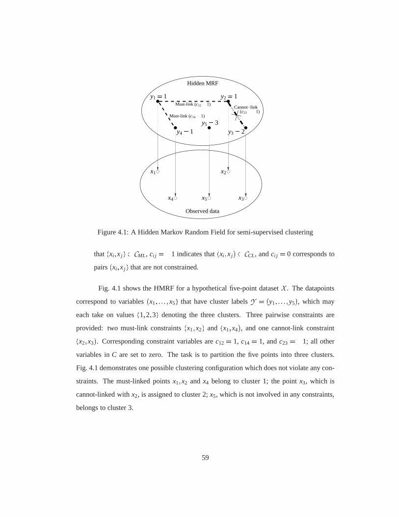
Hidden MRF
Observed data
Cannot−link
x3
x2x1
x5
y2= 1
y4= 1y5= 3
x4
Must-link (c14= 1)
Must-link (c12= 1)
y1= 1
(c23=�1)
y3= 2
Figure 4.1: A Hidden Markov Random Field for semi-supervised clustering
that (xi ;x j) 2 CML, ci j = �1 indicates that(xi ;x j) 2 CCL, andci j = 0 corresponds to
pairs(xi ;x j) that are not constrained.
Fig. 4.1 shows the HMRF for a hypothetical five-point datasetX . The datapoints
correspond to variables(x1; : : : ;x5) that have cluster labelsY = (y1; : : : ;y5), which may
each take on values(1;2;3) denoting the three clusters. Three pairwise constraints are
provided: two must-link constraints(x1;x2) and (x1;x4), and one cannot-link constraint(x2;x3). Corresponding constraint variables arec12 = 1, c14 = 1, andc23 = �1; all other
variables inC are set to zero. The task is to partition the five points into three clusters.
Fig. 4.1 demonstrates one possible clustering configuration which does not violate any con-
straints. The must-linked pointsx1;x2 andx4 belong to cluster 1; the pointx3, which is
cannot-linked withx2, is assigned to cluster 2;x5, which is not involved in any constraints,
belongs to cluster 3.
59
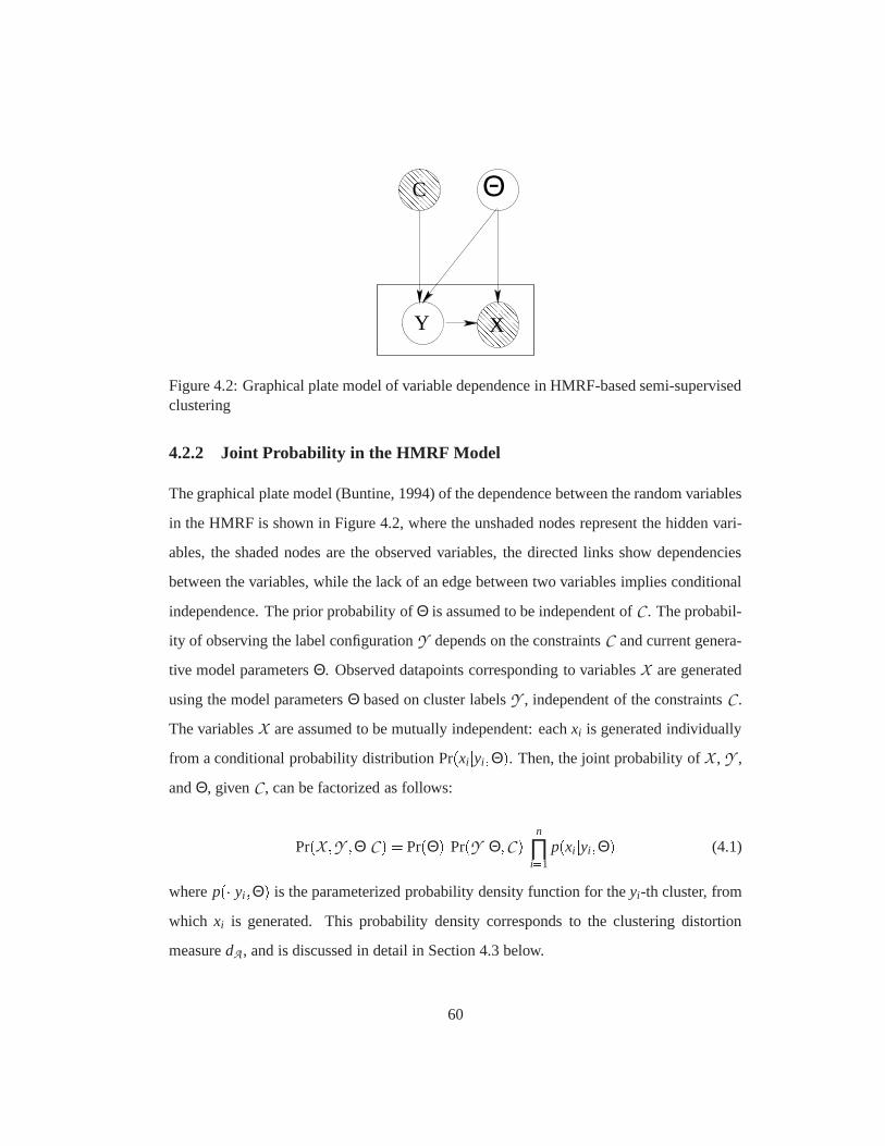
������������������������
������������������������
XY
��������������������
��������������������
C Θ
Figure 4.2: Graphical plate model of variable dependence inHMRF-based semi-supervisedclustering
4.2.2 Joint Probability in the HMRF Model
The graphical plate model (Buntine, 1994) of the dependencebetween the random variables
in the HMRF is shown in Figure 4.2, where the unshaded nodes represent the hidden vari-
ables, the shaded nodes are the observed variables, the directed links show dependencies
between the variables, while the lack of an edge between two variables implies conditional
independence. The prior probability ofΘ is assumed to be independent ofC . The probabil-
ity of observing the label configurationY depends on the constraintsC and current genera-
tive model parametersΘ. Observed datapoints corresponding to variablesX are generated
using the model parametersΘ based on cluster labelsY , independent of the constraintsC .
The variablesX are assumed to be mutually independent: eachxi is generated individually
from a conditional probability distribution Pr(xi jyi ;Θ). Then, the joint probability ofX , Y ,
andΘ, givenC , can be factorized as follows:
Pr(X ;Y ;ΘjC ) = Pr(Θ) Pr(Y jΘ;C ) n
∏i=1
p(xi jyi ;Θ) (4.1)
wherep(�jyi ;Θ) is the parameterized probability density function for theyi-th cluster, from
which xi is generated. This probability density corresponds to the clustering distortion
measuredA , and is discussed in detail in Section 4.3 below.
60
Each hidden random variableyi 2 Y representing the cluster label ofxi 2 X is as-
sociated with a set of neighborsN i , defined as all points to whichxi is must-linked or
cannot-linked:N i = fy j j(xi ;x j) 2 CML[ (xi ;x j) 2 CCLg. We make the Markov assumption
that each labelyi is conditionally independent of all other labels inY given the labels of
its neighbors. The resulting random field over the hidden variablesY is a Markov Ran-
dom Field (MRF), in which by the Hammersley-Clifford theorem (Hammersley & Clifford,
1971) the prior probability of a particular label configuration Y can be expressed as a Gibbs
distribution (Geman & Geman, 1984):
Pr(Y jΘ;C ) = 1Z
exp
�∑i; j v(i; j)! (4.2)
whereZ is the partition function (normalizing term), and eachv(i; j) is the potential function
encoding the compatibility of cluster labelsyi andy j . Because label compatibility is only
relevant for pairs of points that participate in constraints, we definev(i; j) as follows:
v(i; j) =8>>><>>>: wi j fML(i; j) if ci j = 1 andyi 6= y j
wi j fCL(i; j) if ci j =�1 andyi = y j
0 otherwise
(4.3)
where fML and fCL arepenalty functionsthat encode the lowered probability of observing
configurations ofY where must-link and cannot-link constraints are violated respectively,
andwi j is the user-provided constraint weight that can be used to indicate its importance.
Penalty functions are chosen to correlate with the distortion measure by depending on the
distortion measure parametersA , and will be described in detail in Section 4.3 below. Over-
all, this formulation for observing the label assignment (clustering) Y results in higher
probabilities being assigned to configurations in which cluster assignments do not violate
the provided constraints.
61
Then, joint probability on the HMRF can be expressed as follows:
Pr(X ;Y ;ΘjC ) = Pr(Θ)� 1Z
exp
� ∑(i; j):ci j 6=0
v(i; j)!�� n
∏i=1
p(xi jyi ;Θ)� (4.4)
The first factor in the above expression describes a probability distribution over
the model parameters preventing them from attaining degenerate values, thereby providing
regularization. The second factor is the conditional probability of observing a particular
label configuration given the provided constraints, effectively assigning a higher probability
to configurations where the cluster assignments do not violate the constraints. Finally, the
third factor is the conditional probability of generating the observed data points given the
labels and the parameters: if maximum-likelihood estimation (MLE) was performed on the
HMRF, the goal would have been to maximize this term in isolation.
Overall, maximizing the joint HMRF probability in Eq.(4.4)is equivalent to jointly
maximizing the likelihood of generating datapoints from the model and the probability of
label assignments that respect the constraints, while regularizing the model parameters.
4.3 Learnable Similarity Functions in the HMRF Model
The Joint probability formulation in Eq.(4.4) provides a general framework for incorporat-
ing various similarity functions in clustering by choosinga particular form ofp(xi jyi ;Θ),the probability density that generates thei-th instancexi from clusteryi . In this work, we
restrict our attention to probability densities from the exponential family, where the expec-
tation parameter corresponding to clusteryi is µyi , the mean of the points of that cluster.
Using this assumption and the bijection between regular exponential distributions and regu-
lar Bregman divergences (Banerjee et al., 2005b), the conditional density for observed data
can be represented as follows:
p(xi jyi ;Θ) = 1ZΘ
exp��dA(xi ;µyi )�; (4.5)
62
wheredA (xi ;µyi ) is the Bregman divergence betweenxi andµyi , corresponding to the expo-
nential densityp, andZΘ is the normalizer. Different similarity functions can be expressed
via this exponential form:� If xi andµyi are vectors in Euclidean space, anddA is the square of theL2 distance
parameterized by a positive semidefinite weight matrixA , dA(xi ;µyi ) = kxi �µyik2A ,
then the cluster conditional probability is ad-dimensional multivariate normal density
with covariance matrixA�1: p(xi jyi ;Θ) = 1(2π)d=2jAj�1=2 exp(�12(kxi �µyik2
A) (Kearns,
Mansour, & Ng, 1997);� If xi and µyi are probability distributions, anddA is KL-divergence (dA (xi ;µyi ) =∑d
m=1xim log ximµyi m
), then the cluster conditional probability is a multinomial distribu-
tion (Dhillon & Guan, 2003).
The relation in Eq.(4.5) holds even ifdA is not a Bregman divergence but a direc-
tional distance measure such as cosine distance. Then, ifxi andµyi are vectors of unit length
anddA is one minus the dot-product of the vectors�dA (xi ;µyi ) = 1� ∑d
m=1 ximµyi mkxikkµyik �, then the
cluster conditional probability is a von-Mises Fisher (vMF) distribution with unit concen-
tration parameter (Banerjee et al., 2005a), which is the spherical analog of a Gaussian.
Putting Eq.(4.5) into Eq.(4.4) and taking logarithms givesthe following clustering
objective function, minimizing which is equivalent to maximizing the joint probability over
the HMRF in Eq.(4.4):
Jobj = ∑xi2X
dA(xi ;µyi )+ ∑ci j2C
v(i; j)� logPr(Θ)+ logZ+nlogZΘ (4.6)
Thus, an optimal clustering is obtained by minimizingJobj over the hidden variables
Y and parametersΘ, which are comprised of cluster centroidsM and distortion measure
parametersA (note that given cluster assignmentsY , the meansM = fµigKi=1 are uniquely
determined).
63
Selecting an appropriate distortion measuredA for a clustering task typically in-
volves knowledge about properties of the particular domainand dataset. For example,
squared Euclidean distance is most appropriate for low-dimensional data, while cosine
similarity is most fitting for data described by vectors in high-dimensional space where
directional differences are important but vector lengths are irrelevant.
Once a distortion measure is chosen for a given domain, the functions fML and fCL
must be defined to penalize must-link and cannot-link constraint violations respectively,
as described in Section 4.2.2. Each violation penalty is scaled proportionally to the “egre-
giousness” of the violation with respect to the current similarity function. That is, a violated
must-link constraint carries a heavy penalty in the objective function if the distance between
its points is high: this indicates that the two points are highly dissimilar, and the current pa-
rameterization of the similarity function is grossly inadequate. Likewise, two if points of a
violated cannot-link constraints are similar, the penaltyis high since the parameterization
of the similarity function is inappropriate: the points should be dissimilar.
To reflect this intuition, the penalty functions are defined as follows:
fML(i; j) = ϕ(i; j) (4.7)
fCL(i; j) = ϕmax�ϕ(i; j) (4.8)
whereϕ : X�X ! R+ is a non-negative function that penalizes constraint violations, while
ϕmax is an upper bound on the maximum value ofϕ over any pair of points in the dataset;
examples of such bounds for specific distortion functions are described below. The func-
tion ϕ is chosen to be identical or proportional to the distortion measure, assigning higher
penalties to violations of must-link constraints between points that are distant with respect
to the current parameter values of the distortion measure. Conversely, penalties for violated
cannot-link constraints are higher for points that have lowdistance between them. With
this formulation of the penalty functions, constraint violations will lead to changes in the
64
distortion measure parameters that attempt to mend the violations. The potential function
v(i; j) in Eq.(4.3) then becomes:
v(i; j) =8>>><>>>: wi j ϕ(xi ;x j) if ci j = 1 andyi 6= y j
wi j�ϕmax�ϕ(xi;x j)� if ci j =�1 andyi = y j
0 otherwise
; (4.9)
and the objective function for semi-supervised clusteringin Eq.(4.6) can be expressed as:
Jobj = ∑xi2X
dA(xi ;µ(i))+ ∑(xi ;xj )2CMLs:t: yi 6=yj
wi j ϕ(xi ;x j)+ ∑(xi ;xj )2CCLs:t: yi=yj
wi j�ϕmax�ϕ(xi;x j)�� logPr(A)+nlogZΘ (4.10)
Note that the MRF partition function term logZ has been dropped from the objective
function. Its estimation cannot be performed in closed formfor most non-trivial dependency
structures, and while approximate inference methods couldbe employed for computing
it (Kschischang, Frey, & Loeliger, 2001; Wainwright & Jordan, 2003), experiments with the
different methods have shown that minimizing the simplifiedobjective yields comparable
results (Bilenko & Basu, 2004).
4.3.1 Parameter Priors
Following the definition ofΘ in Section 4.2.1, the prior term logPr(Θ) in Eq.(4.6) and the
subsequent equations can be factored as follows:
logPr(Θ) = log�Pr(A)Pr(M )�= logPr(A)+PM
65
where the distortion parametersA are assumed to be independent of the cluster centroids
M = fµigKi=1, and uniform priors are considered over the cluster centroids (leading to the
constant termPM). For different distortion measures, parameter values mayexist that lead
to degenerate solutions of the optimization problem. For example, for squared Euclidean
distance, the zero matrixA= 0 is one such solution. To prevent degenerate solutions, Pr(A)is used to regularize the parameter values using a prior distribution.
If the standard Gaussian prior was used on the parameters of the distortion function,
it would allow the parameters to take negative values. Sinceit is desirable to constrain the
parameter values to be non-negative, it is more appropriateto use the Rayleigh distribu-
tion (Papoulis & Pillai, 2001). Assuming independence of the parametersai 2 A, the prior
term based on the Rayleigh distribution is the following:
Pr(A) = ∏ai2A
ai exp��a2
is2
�s2 (4.11)
wheres is the width parameter.
Next, we consider three examples of commonly used distortion measures and their
parameterizations for use with HMRF-KMEANS: squared Euclidean distance, cosine dis-
tance and KL divergence. Through learning, each of these similarity functions reflects the
correct notion of similarity provided by the pairwise constraints, leading to better clustering
accuracy.
4.3.2 Parameterized Squared Euclidean Distance
Squared Euclidean distance is parameterized using a symmetric positive-definite matrixA
as follows:
deucA(xi ;x j) = kxi �x jk2A = (xi �x j)TA(xi �x j): (4.12)
This form of the parameterized squared Euclidean distance is equivalent to Ma-
66
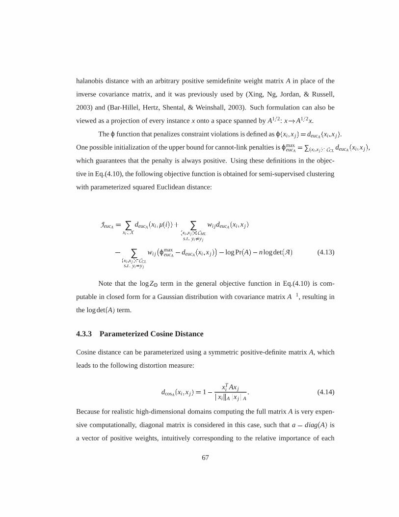
halanobis distance with an arbitrary positive semidefiniteweight matrixA in place of the
inverse covariance matrix, and it was previously used by (Xing, Ng, Jordan, & Russell,
2003) and (Bar-Hillel, Hertz, Shental, & Weinshall, 2003).Such formulation can also be
viewed as a projection of every instancex onto a space spanned byA1=2: x!A1=2x.
Theϕ function that penalizes constraint violations is defined asϕ(xi ;x j)=deucA(xi ;x j).One possible initialization of the upper bound for cannot-link penalties isϕmax
eucA =∑(xi ;xj )2CCLdeucA(xi ;x j),
which guarantees that the penalty is always positive. Usingthese definitions in the objec-
tive in Eq.(4.10), the following objective function is obtained for semi-supervised clustering
with parameterized squared Euclidean distance:
JeucA = ∑xi2X
deucA(xi ;µ(i))+ ∑(xi ;xj )2CMLs:t: yi 6=yj
wi j deucA(xi ;x j)+ ∑(xi ;xj )2CCLs:t: yi=yj
wi j�ϕmax
eucA �deucA(xi ;x j)�� logPr(A)�nlogdet(A) (4.13)
Note that the logZΘ term in the general objective function in Eq.(4.10) is com-
putable in closed form for a Gaussian distribution with covariance matrixA�1, resulting in
the logdet(A) term.
4.3.3 Parameterized Cosine Distance
Cosine distance can be parameterized using a symmetric positive-definite matrixA, which
leads to the following distortion measure:
dcosA(xi ;x j) = 1� xTi AxjkxikAkx jkA
: (4.14)
Because for realistic high-dimensional domains computingthe full matrixA is very expen-
sive computationally, diagonal matrix is considered in this case, such thata = diag(A) is
a vector of positive weights, intuitively corresponding tothe relative importance of each
67
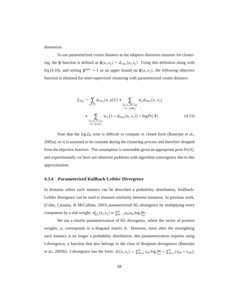
dimension.
To use parameterized cosine distance as the adaptive distortion measure for cluster-
ing, theϕ function is defined asϕ(xi ;x j) = dcosA(xi ;x j). Using this definition along with
Eq.(4.10), and settingϕmax = 1 as an upper bound onϕ(xi ;x j), the following objective
function is obtained for semi-supervised clustering with parameterized cosine distance:
JcosA = ∑xi2X
dcosA(xi ;µ(i))+ ∑(xi ;xj )2CMLs:t: yi 6=yj
wi j dcosA(xi ;x j)+ ∑(xi ;xj )2CCLs:t: yi=yj
wi j�1�dcosA(xi ;x j)�� logPr(A) (4.15)
Note that the logZΘ term is difficult to compute in closed form (Banerjee et al.,
2005a), so it is assumed to be constant during the clusteringprocess and therefore dropped
from the objective function. This assumption is reasonablegiven an appropriate prior Pr(A),and experimentally we have not observed problems with algorithm convergence due to this
approximation.
4.3.4 Parameterized Kullback-Leibler Divergence
In domains where each instance can be described a probability distribution, Kullback-
Leibler divergence can be used to measure similarity between instances. In previous work,
(Cohn, Caruana, & McCallum, 2003) parameterized KL-divergence by multiplying every
component by a real weight:d0KL(xi ;x j) = ∑d
m=1amxim log ximxjm
.
We use a similar parameterization of KL divergence, where the vector of positive
weights, a, corresponds to a diagonal matrixA. However, since after the reweighting
each instance is no longer a probability distribution, thisparameterization requires using
I-divergence, a function that also belongs to the class of Bregman divergences (Banerjee
et al., 2005b). I-divergence has the form:dI (xi ;x j) = ∑dm=1xim log xim
xjm�∑d
m=1(xim� x jm),68
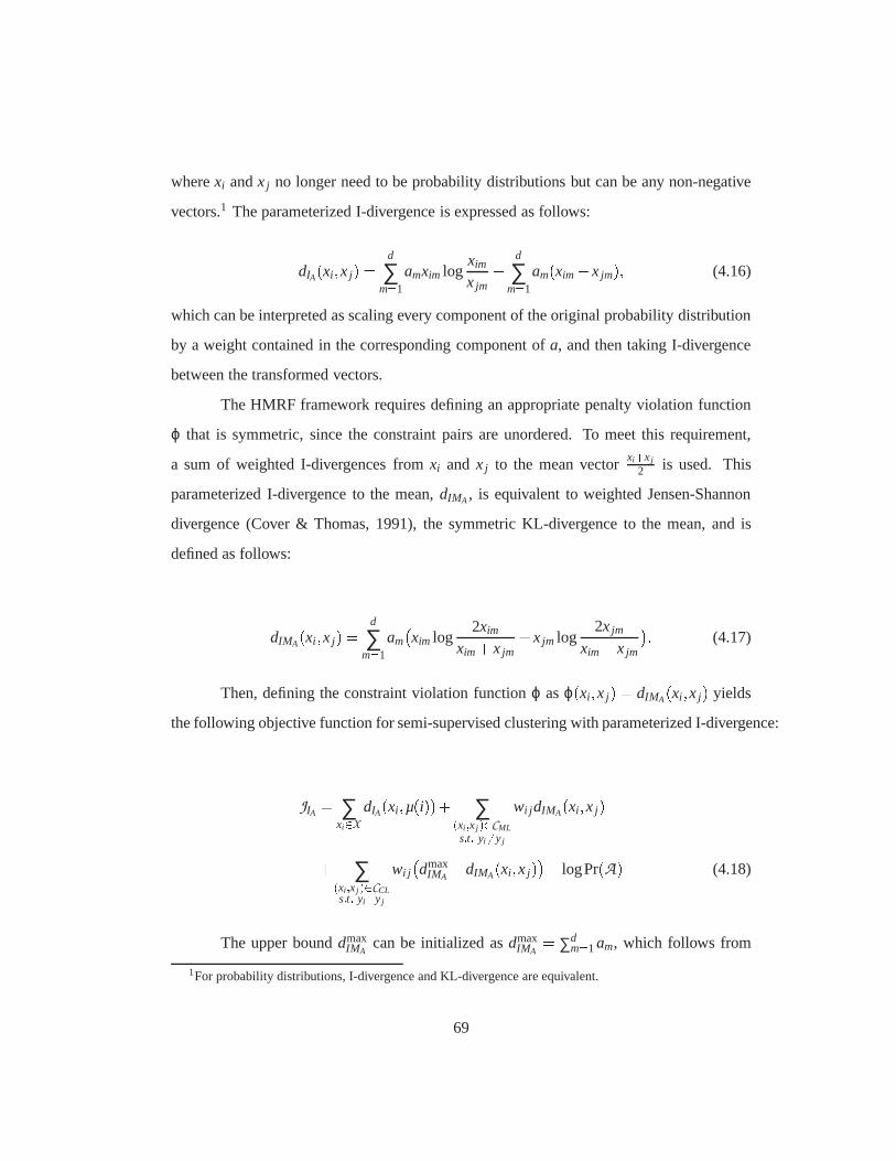
wherexi andx j no longer need to be probability distributions but can be anynon-negative
vectors.1 The parameterized I-divergence is expressed as follows:
dIA(xi ;x j) = d
∑m=1
amxim logxim
x jm� d
∑m=1
am(xim�x jm); (4.16)
which can be interpreted as scaling every component of the original probability distribution
by a weight contained in the corresponding component ofa, and then taking I-divergence
between the transformed vectors.
The HMRF framework requires defining an appropriate penaltyviolation function
ϕ that is symmetric, since the constraint pairs are unordered. To meet this requirement,
a sum of weighted I-divergences fromxi and x j to the mean vectorxi+xj
2 is used. This
parameterized I-divergence to the mean,dIMA, is equivalent to weighted Jensen-Shannon
divergence (Cover & Thomas, 1991), the symmetric KL-divergence to the mean, and is
defined as follows:
dIMA(xi ;x j) = d
∑m=1
am�xim log
2xim
xim+x jm+x jm log
2x jm
xim+x jm
�: (4.17)
Then, defining the constraint violation functionϕ asϕ(xi ;x j) = dIMA(xi ;x j) yields
the following objective function for semi-supervised clustering with parameterized I-divergence:
JIA = ∑xi2X
dIA(xi ;µ(i))+ ∑(xi ;xj )2CMLs:t: yi 6=yj
wi j dIMA(xi ;x j)+ ∑(xi ;xj )2CCLs:t: yi=yj
wi j�dmax
IMA�dIMA(xi ;x j)�� logPr(A) (4.18)
The upper bounddmaxIMA
can be initialized asdmaxIMA
= ∑dm=1am, which follows from
1For probability distributions, I-divergence and KL-divergence are equivalent.
69
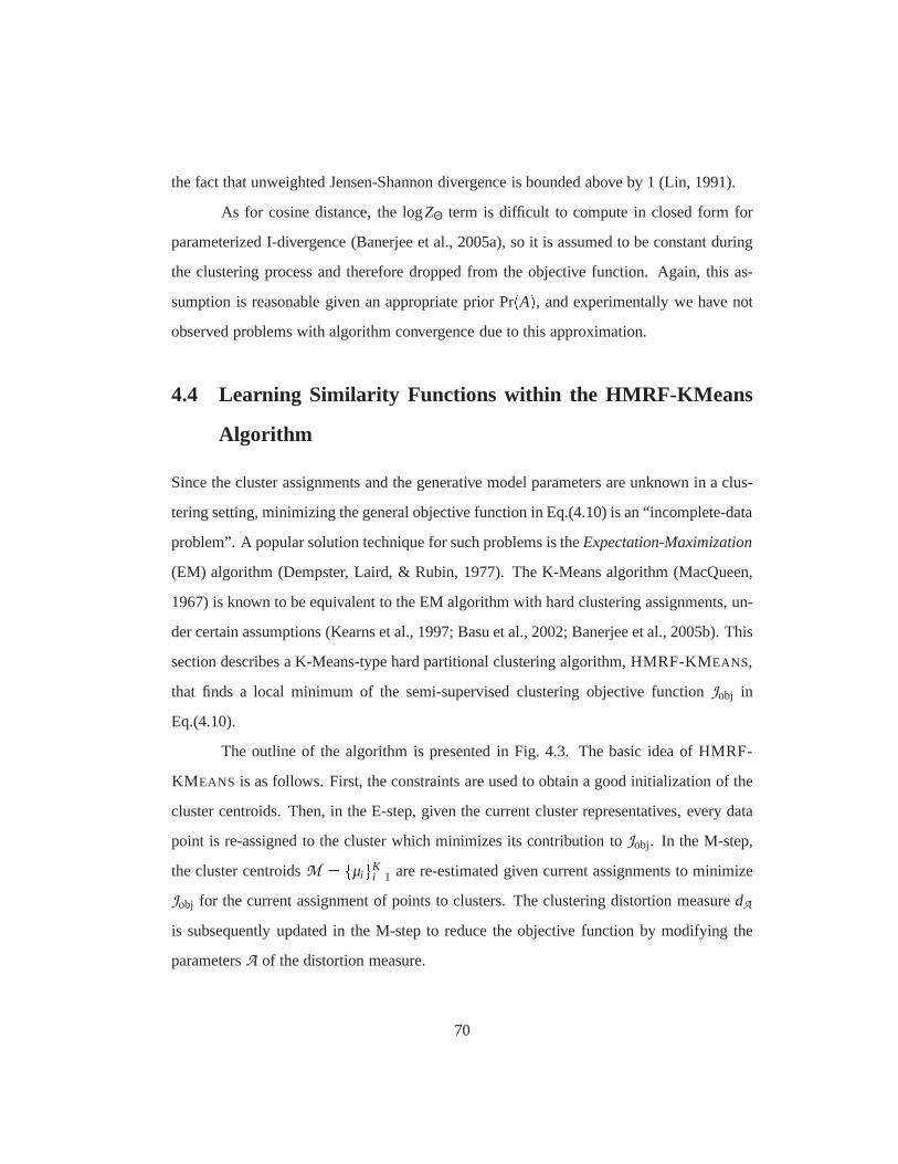
the fact that unweighted Jensen-Shannon divergence is bounded above by 1 (Lin, 1991).
As for cosine distance, the logZΘ term is difficult to compute in closed form for
parameterized I-divergence (Banerjee et al., 2005a), so itis assumed to be constant during
the clustering process and therefore dropped from the objective function. Again, this as-
sumption is reasonable given an appropriate prior Pr(A), and experimentally we have not
observed problems with algorithm convergence due to this approximation.
4.4 Learning Similarity Functions within the HMRF-KMeans
Algorithm
Since the cluster assignments and the generative model parameters are unknown in a clus-
tering setting, minimizing the general objective functionin Eq.(4.10) is an “incomplete-data
problem”. A popular solution technique for such problems istheExpectation-Maximization
(EM) algorithm (Dempster, Laird, & Rubin, 1977). The K-Means algorithm (MacQueen,
1967) is known to be equivalent to the EM algorithm with hard clustering assignments, un-
der certain assumptions (Kearns et al., 1997; Basu et al., 2002; Banerjee et al., 2005b). This
section describes a K-Means-type hard partitional clustering algorithm, HMRF-KMEANS,
that finds a local minimum of the semi-supervised clusteringobjective functionJobj in
Eq.(4.10).
The outline of the algorithm is presented in Fig. 4.3. The basic idea of HMRF-
KM EANS is as follows. First, the constraints are used to obtain a good initialization of the
cluster centroids. Then, in the E-step, given the current cluster representatives, every data
point is re-assigned to the cluster which minimizes its contribution to Jobj. In the M-step,
the cluster centroidsM = fµigKi=1 are re-estimated given current assignments to minimize
Jobj for the current assignment of points to clusters. The clustering distortion measuredA
is subsequently updated in the M-step to reduce the objective function by modifying the
parametersA of the distortion measure.
70
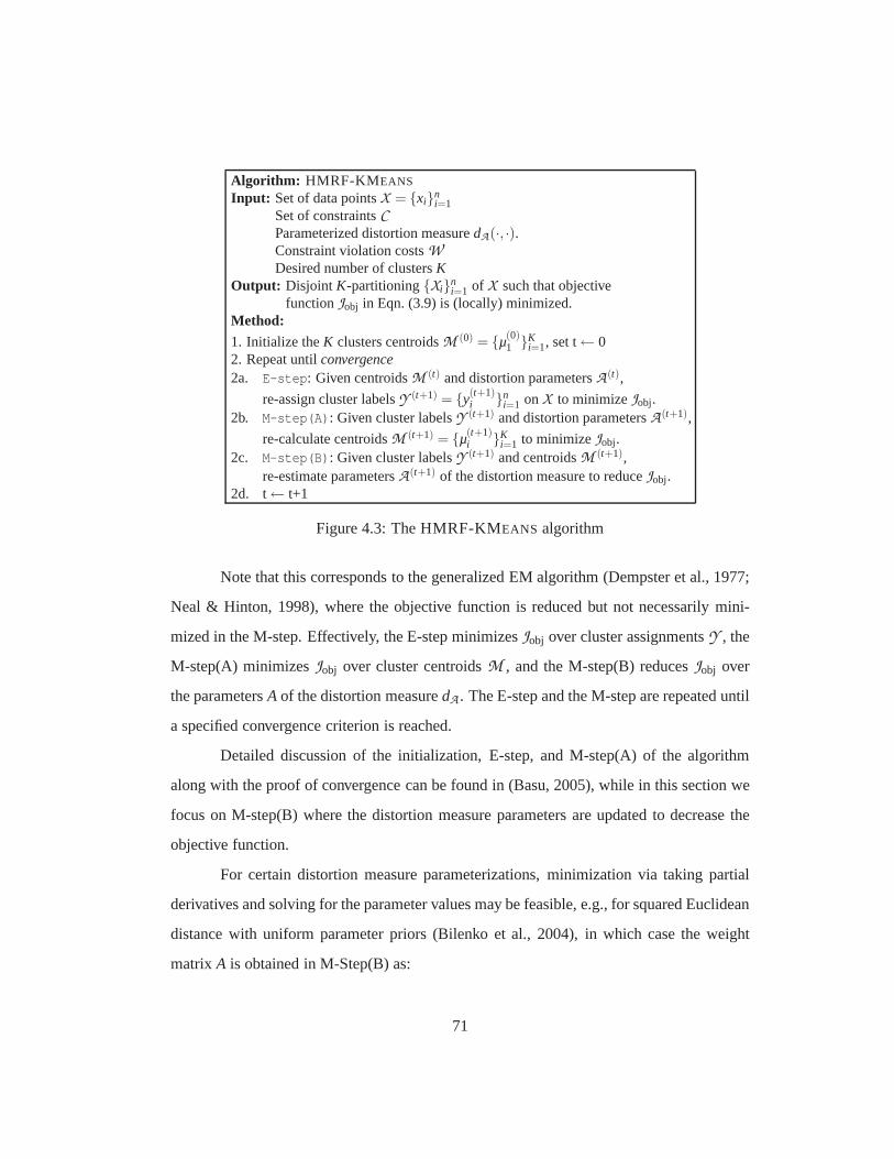
Algorithm: HMRF-KM EANS
Input: Set of data pointsX = {xi}ni=1
Set of constraintsCParameterized distortion measuredA(·, ·).Constraint violation costsWDesired number of clustersK
Output: Disjoint K-partitioning{Xi}ni=1 of X such that objective
functionJobj in Eqn. (3.9) is (locally) minimized.Method:
1. Initialize theK clusters centroidsM (0) = {µ(0)1 }K
i=1, set t← 02. Repeat untilconvergence2a. E-step: Given centroidsM (t) and distortion parametersA(t),
re-assign cluster labelsY (t+1) = {y(t+1)i }n
i=1 on X to minimizeJobj.2b. M-step(A): Given cluster labelsY (t+1) and distortion parametersA(t+1),
re-calculate centroidsM (t+1) = {µ(t+1)i }K
i=1 to minimizeJobj.2c. M-step(B): Given cluster labelsY (t+1) and centroidsM (t+1),
re-estimate parametersA(t+1) of the distortion measure to reduceJobj.2d. t← t+1
Figure 4.3: The HMRF-KMEANS algorithm
Note that this corresponds to the generalized EM algorithm (Dempster et al., 1977;
Neal & Hinton, 1998), where the objective function is reduced but not necessarily mini-
mized in the M-step. Effectively, the E-step minimizesJobj over cluster assignmentsY , the
M-step(A) minimizesJobj over cluster centroidsM , and the M-step(B) reducesJobj over
the parametersA of the distortion measuredA . The E-step and the M-step are repeated until
a specified convergence criterion is reached.
Detailed discussion of the initialization, E-step, and M-step(A) of the algorithm
along with the proof of convergence can be found in (Basu, 2005), while in this section we
focus on M-step(B) where the distortion measure parametersare updated to decrease the
objective function.
For certain distortion measure parameterizations, minimization via taking partial
derivatives and solving for the parameter values may be feasible, e.g., for squared Euclidean
distance with uniform parameter priors (Bilenko et al., 2004), in which case the weight
matrix A is obtained in M-Step(B) as:
71
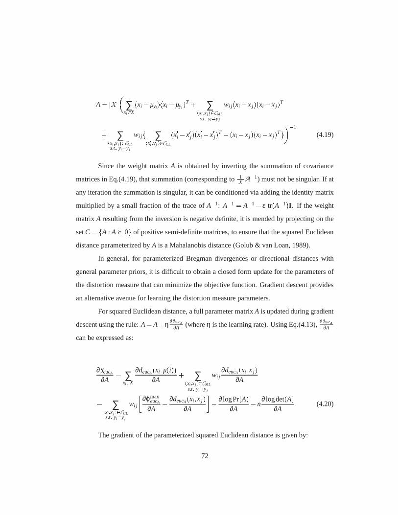
A= jX j�∑xi2X
(xi �µyi )(xi �µyi )T + ∑(xi ;xj )2CMLs:t: yi 6=yj
wi j (xi �x j)(xi �x j)T+ ∑(xi ;xj )2CCLs:t: yi=yj
wi j�
∑(x0i ;x0j )2CCL
(x0i �x0j)(x0i �x0j)T � (xi �x j)(xi �x j)T���1
(4.19)
Since the weight matrixA is obtained by inverting the summation of covariance
matrices in Eq.(4.19), that summation (corresponding to1jX jA�1) must not be singular. If at
any iteration the summation is singular, it can be conditioned via adding the identity matrix
multiplied by a small fraction of the trace ofA�1: A�1 = A�1+ ε tr(A�1)I . If the weight
matrix A resulting from the inversion is negative definite, it is mended by projecting on the
setC = fA : A� 0g of positive semi-definite matrices, to ensure that the squared Euclidean
distance parameterized byA is a Mahalanobis distance (Golub & van Loan, 1989).
In general, for parameterized Bregman divergences or directional distances with
general parameter priors, it is difficult to obtain a closed form update for the parameters of
the distortion measure that can minimize the objective function. Gradient descent provides
an alternative avenue for learning the distortion measure parameters.
For squared Euclidean distance, a full parameter matrixA is updated during gradient
descent using the rule:A=A+η ∂JeucA∂A (whereη is the learning rate). Using Eq.(4.13),
∂JeucA∂A
can be expressed as:
∂JeucA
∂A= ∑
xi2X
∂deucA(xi ;µ(i))∂A
+ ∑(xi ;xj )2CMLs:t: yi 6=yj
wi j∂deucA(xi ;x j)
∂A+ ∑(xi ;xj )2CCLs:t: yi=yj
wi j
�∂ϕmax
eucA
∂A� ∂deucA(xi ;x j)
∂A
�� ∂ logPr(A)∂A
�n∂ logdet(A)
∂A: (4.20)
The gradient of the parameterized squared Euclidean distance is given by:
72
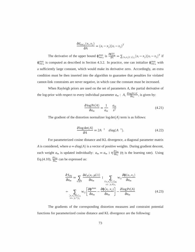
∂deucA(xi ;x j)∂A
= (xi �x j)(xi �x j)T
The derivative of the upper boundϕmaxeucA is
∂ϕmaxeucA
∂A = ∑(xi ;xj )2CCL(xi � x j)(xi � x j)T if
ϕmaxeucA is computed as described in Section 4.3.2. In practice, one can initializeϕmax
eucA with
a sufficiently large constant, which would make its derivative zero. Accordingly, an extra
condition must be then inserted into the algorithm to guarantee that penalties for violated
cannot-link constraints are never negative, in which case the constant must be increased.
When Rayleigh priors are used on the set of parametersA, the partial derivative of
the log-prior with respect to every individual parameteram2 A, ∂ logPr(A)∂am
, is given by:
∂ logPr(A)∂am
= 1am
� am
s2 (4.21)
The gradient of the distortion normalizer logdet(A) term is as follows:
∂ logdet(A)∂A
= 2A�1�diag(A�1): (4.22)
For parameterized cosine distance and KL divergence, a diagonal parameter matrix
A is considered, wherea= diag(A) is a vector of positive weights. During gradient descent,
each weightam is updated individually:am = am+η ∂Jobj
∂am(η is the learning rate). Using
Eq.(4.10),∂Jobj
∂amcan be expressed as:
∂Jobj
∂am= ∑
xi2X
∂dA(xi ;µ(i))∂am
+ ∑(xi ;xj )2CMLs:t: yi 6=yj
wi j∂ϕ(xi ;x j)
∂am+ ∑(xi ;xj )2CCLs:t: yi=yj
wi j
�∂ϕmax
∂am� ∂ϕ(xi ;x j)
∂am
�� ∂ logPr(A)∂am
(4.23)
The gradients of the corresponding distortion measures andconstraint potential
functions for parameterized cosine distance and KL divergence are the following:
73
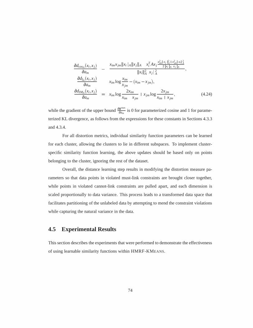
∂dcosA(xi ;x j)∂am
= ximx jmkxikAkx jkA�xTi Axj
x2imkxj k2
A+x2jmkxik2
A
2kxikAkxjkAkxik2Akx jk2
A
;∂dIA(xi ;x j)
∂am= xim log
xim
x jm� (xim�x jm);
∂dIMA(xi ;x j)∂am
= xim log2xim
xim+x jm+x jm log
2x jm
xim+x jm; (4.24)
while the gradient of the upper bound∂ϕmax
∂amis 0 for parameterized cosine and 1 for parame-
terized KL divergence, as follows from the expressions for these constants in Sections 4.3.3
and 4.3.4.
For all distortion metrics, individual similarity function parameters can be learned
for each cluster, allowing the clusters to lie in different subspaces. To implement cluster-
specific similarity function learning, the above updates should be based only on points
belonging to the cluster, ignoring the rest of the dataset.
Overall, the distance learning step results in modifying the distortion measure pa-
rameters so that data points in violated must-link constraints are brought closer together,
while points in violated cannot-link constraints are pulled apart, and each dimension is
scaled proportionally to data variance. This process leadsto a transformed data space that
facilitates partitioning of the unlabeled data by attempting to mend the constraint violations
while capturing the natural variance in the data.
4.5 Experimental Results
This section describes the experiments that were performedto demonstrate the effectiveness
of using learnable similarity functions within HMRF-KMEANS.
74
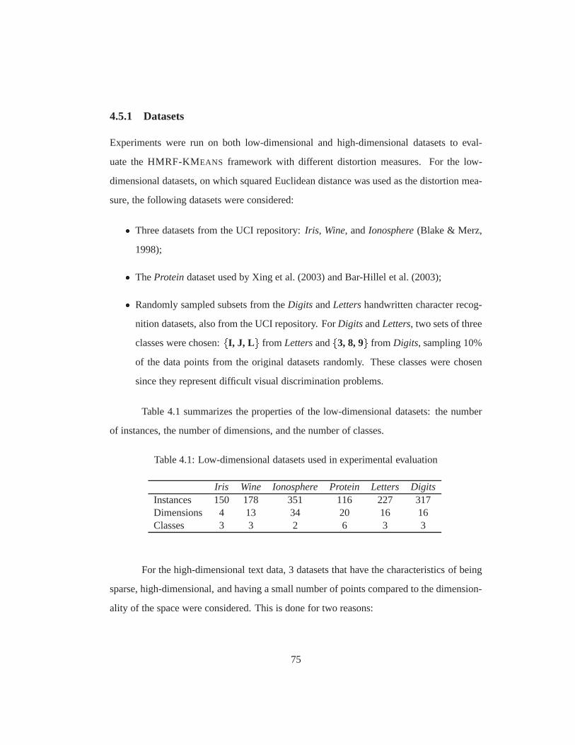
4.5.1 Datasets
Experiments were run on both low-dimensional and high-dimensional datasets to eval-
uate the HMRF-KMEANS framework with different distortion measures. For the low-
dimensional datasets, on which squared Euclidean distancewas used as the distortion mea-
sure, the following datasets were considered:� Three datasets from the UCI repository:Iris, Wine, andIonosphere(Blake & Merz,
1998);� TheProteindataset used by Xing et al. (2003) and Bar-Hillel et al. (2003);� Randomly sampled subsets from theDigits andLettershandwritten character recog-
nition datasets, also from the UCI repository. ForDigits andLetters, two sets of three
classes were chosen:fI, J, L g from Lettersandf3, 8, 9g from Digits, sampling 10%
of the data points from the original datasets randomly. These classes were chosen
since they represent difficult visual discrimination problems.
Table 4.1 summarizes the properties of the low-dimensionaldatasets: the number
of instances, the number of dimensions, and the number of classes.
Table 4.1: Low-dimensional datasets used in experimental evaluation
Iris Wine Ionosphere Protein Letters DigitsInstances 150 178 351 116 227 317Dimensions 4 13 34 20 16 16Classes 3 3 2 6 3 3
For the high-dimensional text data, 3 datasets that have thecharacteristics of being
sparse, high-dimensional, and having a small number of points compared to the dimension-
ality of the space were considered. This is done for two reasons:
75
� When clustering sparse high-dimensional data, e.g., text documents represented us-
ing the vector space model, it is particularly difficult to cluster small datasets, as
observed by Dhillon and Guan (2003). The purpose of performing experiments on
these subsets is to scale down the sizes of the datasets for computational reasons but
at the same time not scale down the difficulty of the tasks.� Clustering small number of sparse high-dimensional data points is a likely scenario
in realistic applications. For example, when clustering the search results in a web-
search engine like Vivısimo2, the number of webpages that are being clustered is
typically in the order of hundreds. However, the dimensionality of the feature space,
corresponding to the number of unique words in all the webpages, is in the order of
thousands. Moreover, each webpage is sparse, since it contains only a small number
of all the possible words. On such datasets, clustering algorithms can easily get stuck
in local optima: in such cases it has been observed that thereis little relocation of
documents between clusters for most initializations, which leads to poor clustering
quality after convergence of the algorithm (Dhillon & Guan,2003). Supervision in
the form of pairwise constraints is most beneficial in such cases and may significantly
improve clustering quality.
Three datasets were derived from the20-Newsgroupscollection.3 This collection
has messages harvested from 20 different Usenet newsgroups, 1000 messages from each
newsgroup. From the original dataset, a reduced dataset wascreated by taking a random
subsample of 100 documents from each of the 20 newsgroups. Three datasets were cre-
ated by selecting 3 categories from the reduced collection.News-Similar-3consists of 3
newsgroups on similar topics (comp.graphics, comp.os.ms-windows, comp.windows.x)
with significant overlap between clusters due to cross-posting. News-Related-3consists
of 3 newsgroups on related topics (talk.politics.misc, talk.politics.guns, and
2http://www.vivisimo.com3http://www.ai.mit.edu/people/jrennie/20Newsgroups
76
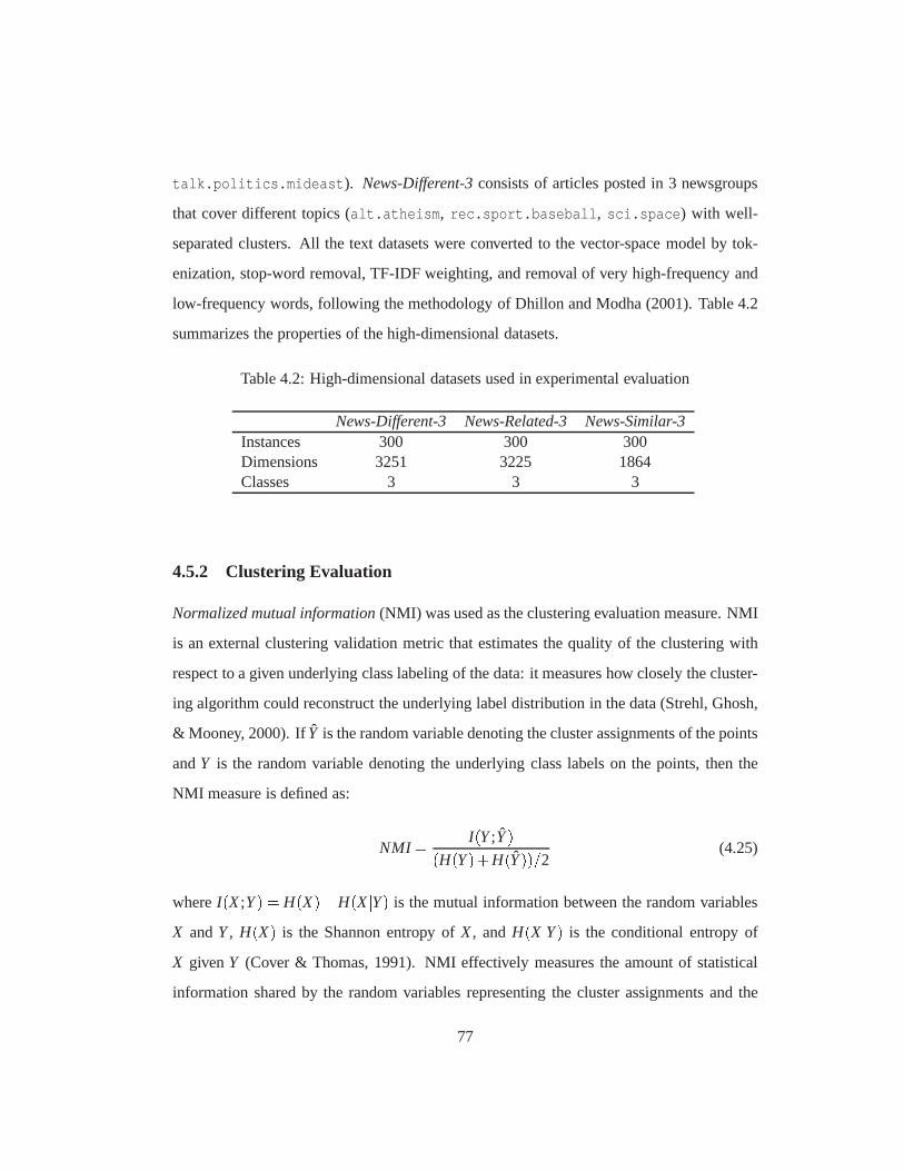
talk.politics.mideast). News-Different-3consists of articles posted in 3 newsgroups
that cover different topics (alt.atheism, rec.sport.baseball, sci.space) with well-
separated clusters. All the text datasets were converted tothe vector-space model by tok-
enization, stop-word removal, TF-IDF weighting, and removal of very high-frequency and
low-frequency words, following the methodology of Dhillonand Modha (2001). Table 4.2
summarizes the properties of the high-dimensional datasets.
Table 4.2: High-dimensional datasets used in experimentalevaluation
News-Different-3 News-Related-3 News-Similar-3Instances 300 300 300Dimensions 3251 3225 1864Classes 3 3 3
4.5.2 Clustering Evaluation
Normalized mutual information(NMI) was used as the clustering evaluation measure. NMI
is an external clustering validation metric that estimatesthe quality of the clustering with
respect to a given underlying class labeling of the data: it measures how closely the cluster-
ing algorithm could reconstruct the underlying label distribution in the data (Strehl, Ghosh,
& Mooney, 2000). IfY is the random variable denoting the cluster assignments of the points
andY is the random variable denoting the underlying class labelson the points, then the
NMI measure is defined as:
NMI = I(Y;Y)(H(Y)+H(Y))=2(4.25)
whereI(X;Y) = H(X)�H(XjY) is the mutual information between the random variables
X andY, H(X) is the Shannon entropy ofX, andH(XjY) is the conditional entropy of
X givenY (Cover & Thomas, 1991). NMI effectively measures the amountof statistical
information shared by the random variables representing the cluster assignments and the
77
user-labeled class assignments of the data points. Though various clustering evaluation
measures have been used in the literature, NMI and it’s variants have become popular lately
among clustering practitioners (Dom, 2001; Fern & Brodley,2003; Meila, 2003).
4.5.3 Methodology
Learning curves were generated using two-fold cross-validation performed over 20 runs on
each dataset. In every trial, 50% of the dataset was set asideas the training fold. Every point
on the learning curve corresponds to the number of constraints on pairs of data points from
the training fold. These constraints are obtained by randomly selecting pairs of points from
the training fold and creating must-link or cannot-link constraints depending on whether the
underlying classes of the two points are the same or different. Unit constraint costsW were
used for all constraints (original and inferred), since thedatasets did not provide individual
weights for the constraints. The gradient step sizeη for learning the distortion measure
parameters and the Rayleigh prior width parameters were set based on pilot studies. The
gradient step size was set toη = 100:0 for clustering with weighted cosine distancedcosA
andη = 0:08 for weighted I divergencedIA. The Rayleigh prior width parameter was set
to s= 1. In a real-life setting, the free parameters of the algorithm could be tuned using
cross-validation with a hold-out set. The clustering algorithm was run on the whole dataset,
but NMI was calculated using points in the test fold.
Sensitivity experiments were performed with HMRF-KMEANS to study the ef-
fectiveness of employing learnable similarity functions.The proposed HMRF-KMEANS
algorithm was compared with three ablations, as well as withunsupervised K-Means clus-
tering. The following variants were compared for distortion measuresdcosA, dIA anddeucA :� HMRF-KMEANS-C-D-R is the complete HMRF-KMEANS algorithm that incor-
porates constraints in cluster assignments (C), performs distortion measure learning
(D), and also performs regularization (R) using a Rayleigh prior as described in Sec-
tion 4.3.1;
78
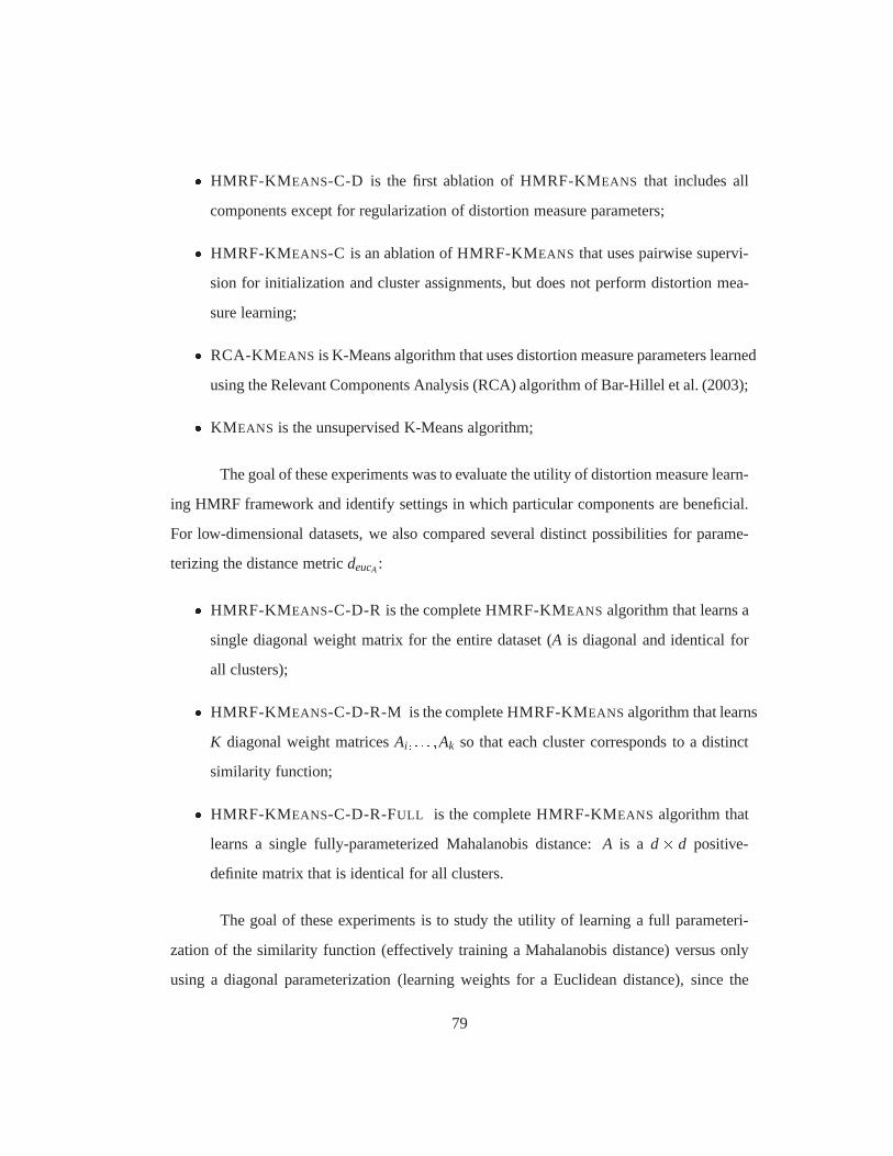
� HMRF-KMEANS-C-D is the first ablation of HMRF-KMEANS that includes all
components except for regularization of distortion measure parameters;� HMRF-KMEANS-C is an ablation of HMRF-KMEANS that uses pairwise supervi-
sion for initialization and cluster assignments, but does not perform distortion mea-
sure learning;� RCA-KMEANS is K-Means algorithm that uses distortion measure parameters learned
using the Relevant Components Analysis (RCA) algorithm of Bar-Hillel et al. (2003);� KM EANS is the unsupervised K-Means algorithm;
The goal of these experiments was to evaluate the utility of distortion measure learn-
ing HMRF framework and identify settings in which particular components are beneficial.
For low-dimensional datasets, we also compared several distinct possibilities for parame-
terizing the distance metricdeucA:� HMRF-KMEANS-C-D-R is the complete HMRF-KMEANS algorithm that learns a
single diagonal weight matrix for the entire dataset (A is diagonal and identical for
all clusters);� HMRF-KMEANS-C-D-R-M is the complete HMRF-KMEANS algorithm that learns
K diagonal weight matricesAi; : : : ;Ak so that each cluster corresponds to a distinct
similarity function;� HMRF-KMEANS-C-D-R-FULL is the complete HMRF-KMEANS algorithm that
learns a single fully-parameterized Mahalanobis distance: A is a d� d positive-
definite matrix that is identical for all clusters.
The goal of these experiments is to study the utility of learning a full parameteri-
zation of the similarity function (effectively training a Mahalanobis distance) versus only
using a diagonal parameterization (learning weights for a Euclidean distance), since the
79
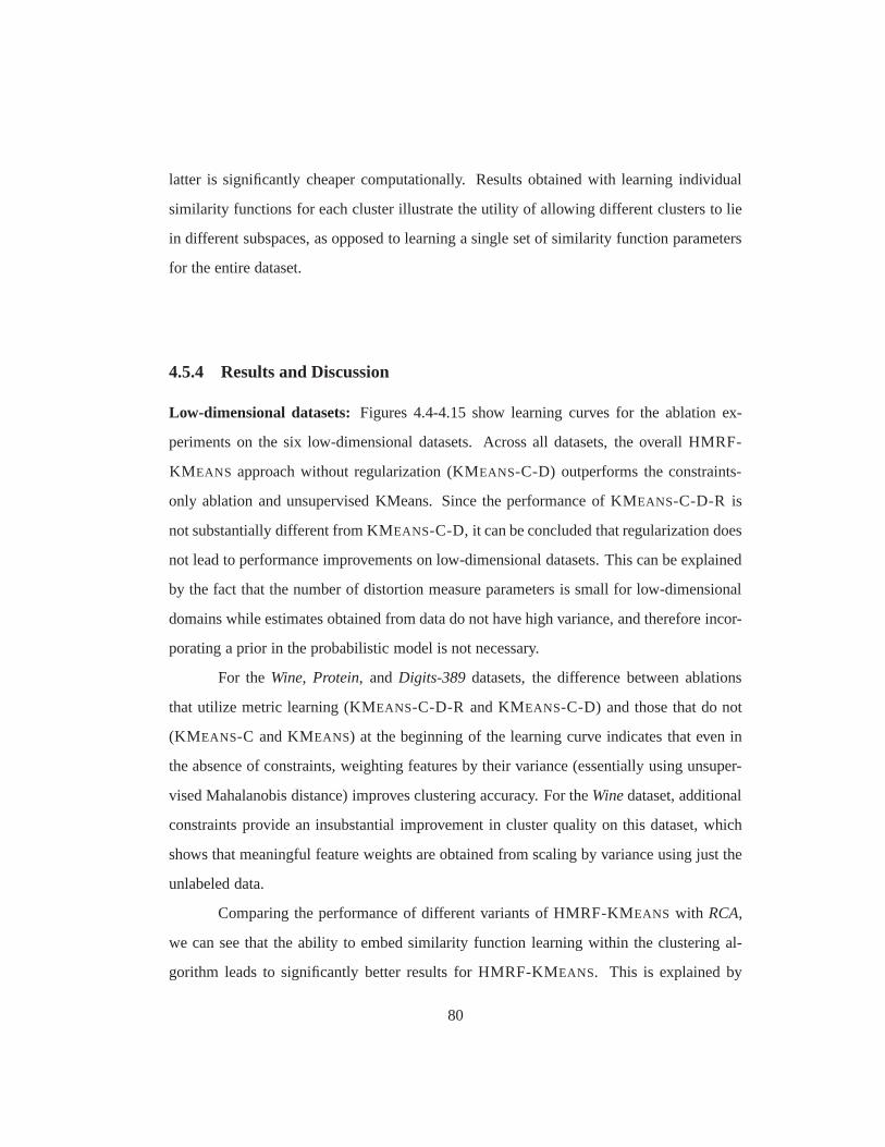
latter is significantly cheaper computationally. Results obtained with learning individual
similarity functions for each cluster illustrate the utility of allowing different clusters to lie
in different subspaces, as opposed to learning a single set of similarity function parameters
for the entire dataset.
4.5.4 Results and Discussion
Low-dimensional datasets: Figures 4.4-4.15 show learning curves for the ablation ex-
periments on the six low-dimensional datasets. Across all datasets, the overall HMRF-
KM EANS approach without regularization (KMEANS-C-D) outperforms the constraints-
only ablation and unsupervised KMeans. Since the performance of KMEANS-C-D-R is
not substantially different from KMEANS-C-D, it can be concluded that regularization does
not lead to performance improvements on low-dimensional datasets. This can be explained
by the fact that the number of distortion measure parametersis small for low-dimensional
domains while estimates obtained from data do not have high variance, and therefore incor-
porating a prior in the probabilistic model is not necessary.
For theWine, Protein, andDigits-389 datasets, the difference between ablations
that utilize metric learning (KMEANS-C-D-R and KMEANS-C-D) and those that do not
(KM EANS-C and KMEANS) at the beginning of the learning curve indicates that even in
the absence of constraints, weighting features by their variance (essentially using unsuper-
vised Mahalanobis distance) improves clustering accuracy. For theWinedataset, additional
constraints provide an insubstantial improvement in cluster quality on this dataset, which
shows that meaningful feature weights are obtained from scaling by variance using just the
unlabeled data.
Comparing the performance of different variants of HMRF-KMEANS with RCA,
we can see that the ability to embed similarity function learning within the clustering al-
gorithm leads to significantly better results for HMRF-KMEANS. This is explained by
80
0.74
0.76
0.78
0.8
0.82
0.84
0.86
0.88
0 100 200 300 400 500
NM
I
Number of Constraints
HMRF-KMeans-C-D-RHMRF-KMeans-C-D
HMRF-KMeans-CRCA-KMeans
KMeans
Figure 4.4: Results fordeuc on theIris dataset
0.55
0.6
0.65
0.7
0.75
0.8
0.85
0.9
0.95
0 100 200 300 400 500
NM
I
Number of Constraints
HMRF-KMeans-C-D-RHMRF-KMeans-C-D-R-M
HMRF-KMeans-C-D-R-Full
Figure 4.5: Results fordeuc on theIris dataset with fulland per-cluster parameterizations
81
0.4
0.45
0.5
0.55
0.6
0.65
0.7
0.75
0.8
0.85
0.9
0 100 200 300 400 500
NM
I
Number of Constraints
HMRF-KMeans-C-D-RHMRF-KMeans-C-D
HMRF-KMeans-CRCA-KMeans
KMeans
Figure 4.6: Results fordeuc on theWinedataset
0.45
0.5
0.55
0.6
0.65
0.7
0.75
0.8
0.85
0.9
0.95
0 100 200 300 400 500
NM
I
Number of Constraints
HMRF-KMeans-C-D-RHMRF-KMeans-C-D-R-M
HMRF-KMeans-C-D-R-Full
Figure 4.7: Results fordeuc on theWinedataset withfull and per-cluster parameterizations
82

0.44
0.46
0.48
0.5
0.52
0.54
0.56
0.58
0.6
0.62
0.64
0 100 200 300 400 500
NM
I
Number of Constraints
HMRF-KMeans-C-D-RHMRF-KMeans-C-D
HMRF-KMeans-CRCA-KMeans
KMeans
Figure 4.8: Results fordeuc on theProteindataset
0.3
0.35
0.4
0.45
0.5
0.55
0.6
0.65
0 100 200 300 400 500
NM
I
Number of Constraints
HMRF-KMeans-C-D-RHMRF-KMeans-C-D-R-M
HMRF-KMeans-C-D-R-Full
Figure 4.9: Results fordeuc on theProteindataset withfull and per-cluster parameterizations
83
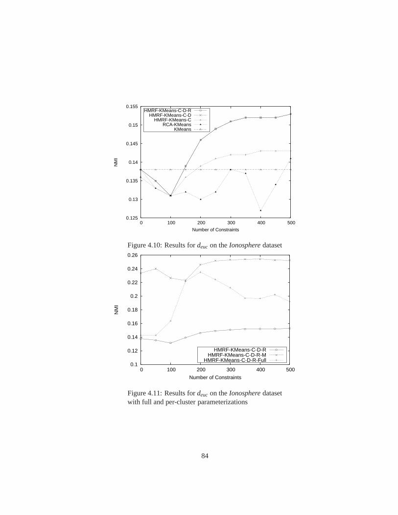
0.125
0.13
0.135
0.14
0.145
0.15
0.155
0 100 200 300 400 500
NM
I
Number of Constraints
HMRF-KMeans-C-D-RHMRF-KMeans-C-D
HMRF-KMeans-CRCA-KMeans
KMeans
Figure 4.10: Results fordeuc on theIonospheredataset
0.1
0.12
0.14
0.16
0.18
0.2
0.22
0.24
0.26
0 100 200 300 400 500
NM
I
Number of Constraints
HMRF-KMeans-C-D-RHMRF-KMeans-C-D-R-M
HMRF-KMeans-C-D-R-Full
Figure 4.11: Results fordeuc on theIonospheredatasetwith full and per-cluster parameterizations
84

0.55
0.6
0.65
0.7
0.75
0.8
0 100 200 300 400 500
NM
I
Number of Constraints
HMRF-KMeans-C-D-RHMRF-KMeans-C-D
HMRF-KMeans-CRCA-KMeans
KMeans
Figure 4.12: Results fordeuc on theDigits-389dataset
0.55
0.6
0.65
0.7
0.75
0.8
0.85
0 100 200 300 400 500
NM
I
Number of Constraints
HMRF-KMeans-C-D-RHMRF-KMeans-C-D-R-M
HMRF-KMeans-C-D-R-Full
Figure 4.13: Results fordeuc on theDigits-389datasetwith full and per-cluster parameterizations
85
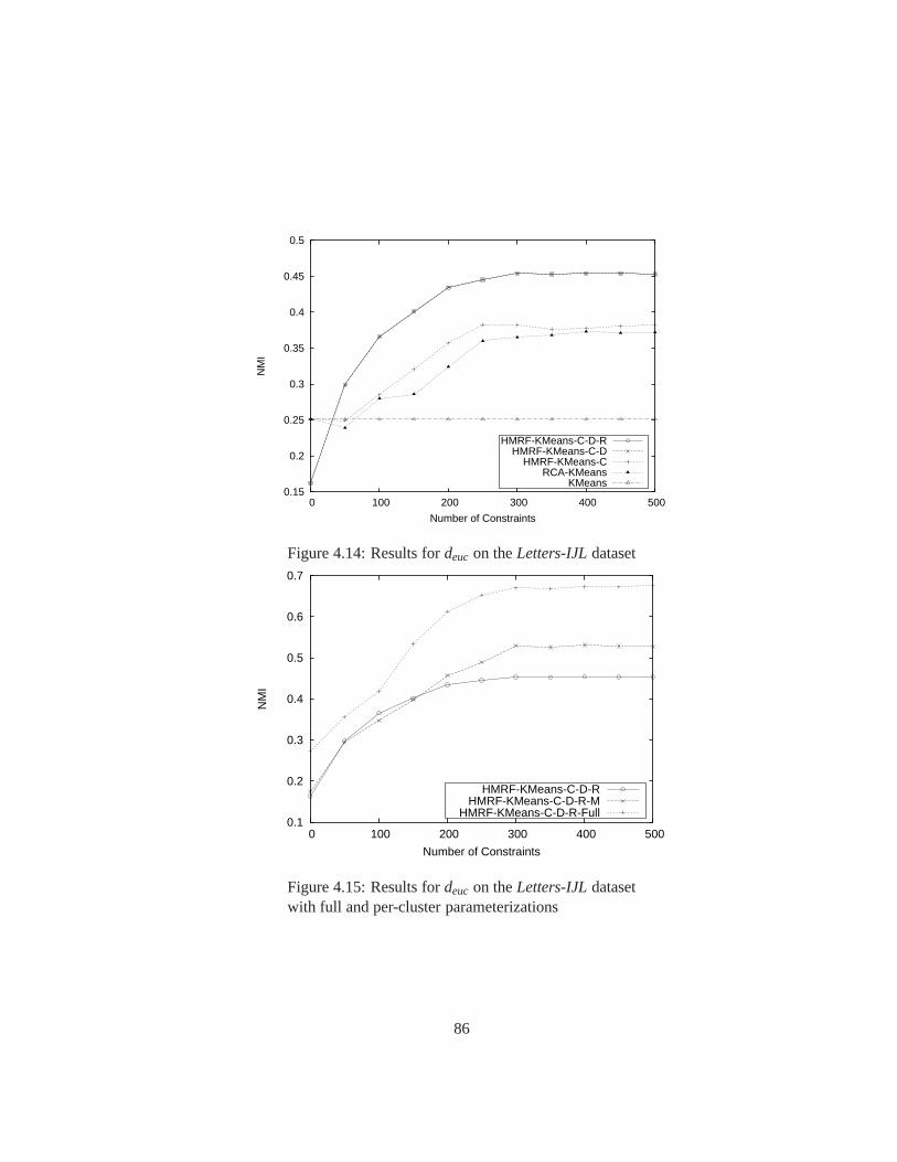
0.15
0.2
0.25
0.3
0.35
0.4
0.45
0.5
0 100 200 300 400 500
NM
I
Number of Constraints
HMRF-KMeans-C-D-RHMRF-KMeans-C-D
HMRF-KMeans-CRCA-KMeans
KMeans
Figure 4.14: Results fordeuc on theLetters-IJLdataset
0.1
0.2
0.3
0.4
0.5
0.6
0.7
0 100 200 300 400 500
NM
I
Number of Constraints
HMRF-KMeans-C-D-RHMRF-KMeans-C-D-R-M
HMRF-KMeans-C-D-R-Full
Figure 4.15: Results fordeuc on theLetters-IJLdatasetwith full and per-cluster parameterizations
86
the fact thatRCAutilizes only the pairwise constraints for learning the similarity function
parameters, while HMRF-KMEANS uses both the constraints and the unlabeled data, ad-
justing the parameters gradually in the course of clustering.
The results for learning full-matrix and per-cluster parameterizations of the similar-
ity function demonstrate that both of these extensions can lead to significant improvements
in clustering quality. However, the relative usefulness ofthese two techniques varies be-
tween the datasets. Multiple similarity functions are beneficial for all datasets except for
Proteinwhere they did not affect the results, andIris, where they had a negative effect. Us-
ing the full matrix parameterization also did not affectProtein results, and had a negative
effect onDigits, while it improved results on the other four datasets. This inconsistency can
be explained by the fact that the relative success of the two techniques depends on the prop-
erties of a particular dataset: using a full weight matrix helps when the features are highly
correlated, while using per-cluster parameterization lead to improvements when clusters in
the dataset are of different shapes or lie in different subspaces of the original space. A
combination of the two techniques is most helpful when both of these requirements are
satisfied, as forWineandLetters, which was observed by visualizing low-dimensional pro-
jections of these datasets. For other datasets with the exception ofProtein, either per-cluster
parameterization or the full weight matrix lead to maximum performance in isolation.
Some of the HMRF-KMEANS learning curves display a characteristic “dip”, where
clustering accuracy decreases as a few initial constraintsare provided, but after a certain
point starts to increase and eventually rises above the initial point on the learning curve.
One possible explanation of this phenomenon is overfitting:having just a few constraints
provides unreliable supervision, forcing the algorithm toconverge to inferior local op-
tima, while increasing the number of provided constraints allows overcoming this effect.
Overall, when both constraints and distortion measure learning are utilized, the unified ap-
proach benefits from the individual strengths of the two methods, as can be seen from the
KM EANS-C-D results.
87
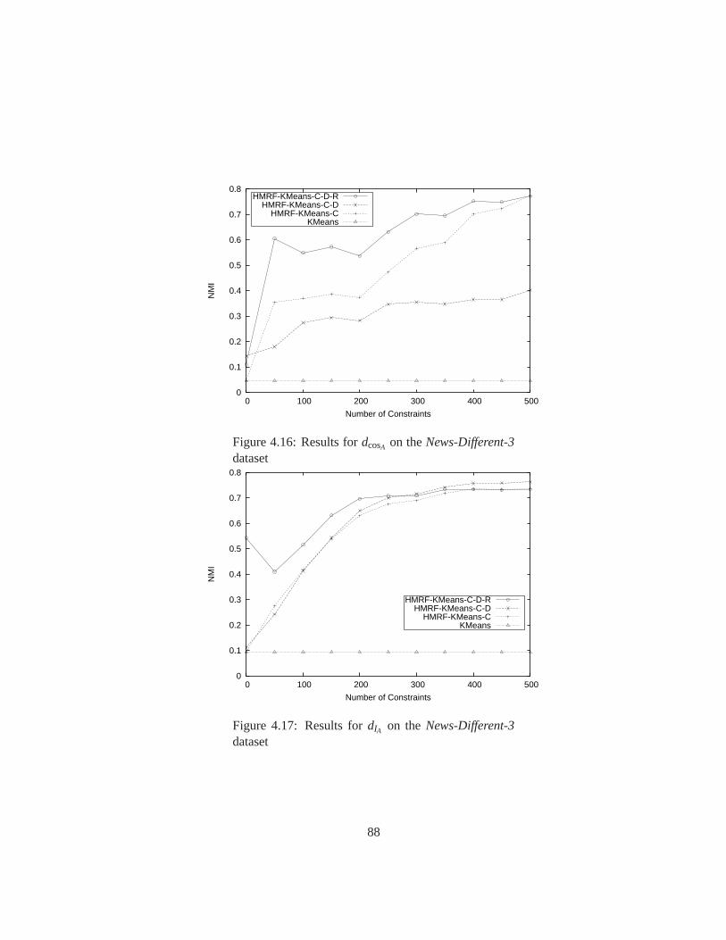
0
0.1
0.2
0.3
0.4
0.5
0.6
0.7
0.8
0 100 200 300 400 500
NM
I
Number of Constraints
HMRF-KMeans-C-D-RHMRF-KMeans-C-D
HMRF-KMeans-CKMeans
Figure 4.16: Results fordcosA on theNews-Different-3dataset
0
0.1
0.2
0.3
0.4
0.5
0.6
0.7
0.8
0 100 200 300 400 500
NM
I
Number of Constraints
HMRF-KMeans-C-D-RHMRF-KMeans-C-D
HMRF-KMeans-CKMeans
Figure 4.17: Results fordIA on theNews-Different-3dataset
88
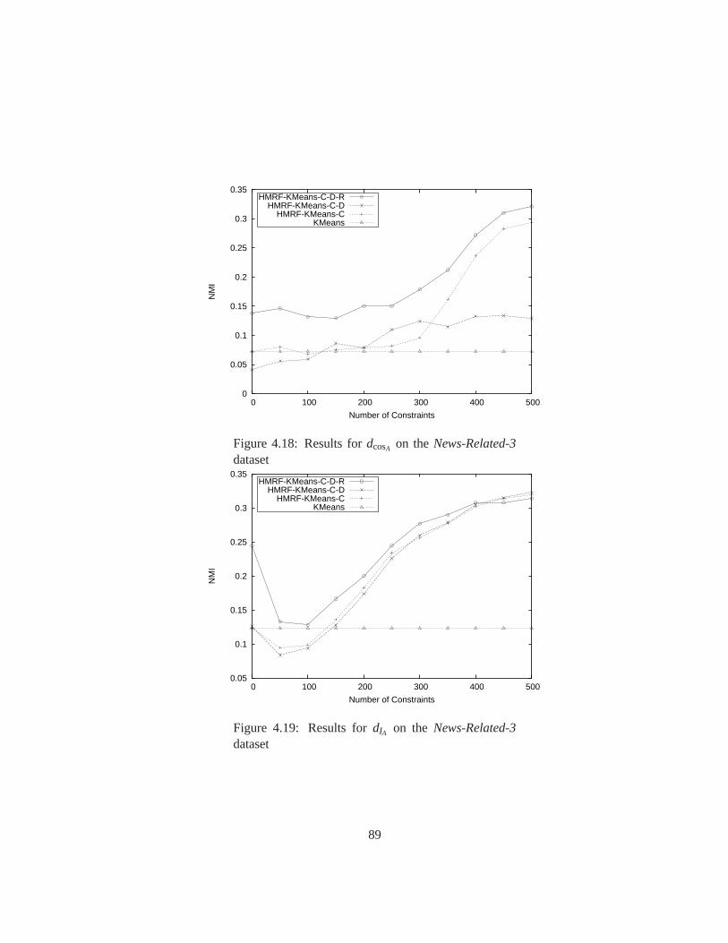
0
0.05
0.1
0.15
0.2
0.25
0.3
0.35
0 100 200 300 400 500
NM
I
Number of Constraints
HMRF-KMeans-C-D-RHMRF-KMeans-C-D
HMRF-KMeans-CKMeans
Figure 4.18: Results fordcosA on theNews-Related-3dataset
0.05
0.1
0.15
0.2
0.25
0.3
0.35
0 100 200 300 400 500
NM
I
Number of Constraints
HMRF-KMeans-C-D-RHMRF-KMeans-C-D
HMRF-KMeans-CKMeans
Figure 4.19: Results fordIA on the News-Related-3dataset
89
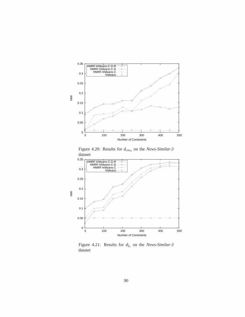
0
0.05
0.1
0.15
0.2
0.25
0.3
0.35
0 100 200 300 400 500
NM
I
Number of Constraints
HMRF-KMeans-C-D-RHMRF-KMeans-C-D
HMRF-KMeans-CKMeans
Figure 4.20: Results fordcosA on theNews-Similar-3dataset
0
0.05
0.1
0.15
0.2
0.25
0.3
0.35
0 100 200 300 400 500
NM
I
Number of Constraints
HMRF-KMeans-C-D-RHMRF-KMeans-C-D
HMRF-KMeans-CKMeans
Figure 4.21: Results fordIA on the News-Similar-3dataset
90
High-dimensional datasets: Figures 4.16, 4.18 and 4.20 present the results for
the ablation experiments where weighted cosine similaritydcosA was used as the distortion
measure, while Figures 4.17, 4.19 and 4.21 summarize experiments where weighted I di-
vergencedIA was used.
As the results demonstrate, the full HMRF-KMEANS algorithm with regularization
(KM EANS-C-D-R) outperforms the unsupervised K-Means baseline as well as the ablated
versions of the algorithm for both distortion measuresdcosA anddIA. As can be seen from
results for zero pairwise constraints in Figs. 4.16-4.21, distortion measure learning is bene-
ficial even in the absence of any pairwise constraints, sinceit allows capturing the relative
importance of the different attributes in the unsuperviseddata. In the absence of super-
vised data or when no constraints are violated, distance learning attempts to minimize the
objective function by adjusting the weights given the distortion between the unsupervised
datapoints and their corresponding cluster representatives.
For high-dimensional datasets, regularization is clearlybeneficial to performance,
as can be seen from the improved performance of KMEANS-C-D-R over KMEANS-C-D
on all datasets. This can be explained by the fact that the number of distortion measure
parameters is large for high-dimensional datasets, and therefore algorithm-based estimates
of parameters tend to be unreliable unless they incorporatea prior.
Overall, the experimental results demonstrate that learning similarity functions within
the HMRF-KMEANS algorithm lead to significant improvements in clustering accuracy,
effectively exploiting both supervision in the form of pairwise constraints and the unsuper-
vised data.
4.6 Related Work
Several semi-supervised clustering approaches were proposed that incorporate adaptive dis-
tortion measures, including parameterizations of Jensen-Shannon divergence (Cohn et al.,
2003) as well as Euclidean and Mahalanobis distances (Klein, Kamvar, & Manning, 2002;
91
Bar-Hillel et al., 2003; Xing et al., 2003). These techniques use only constraints to learn
the distortion measure parameters and ignore unlabeled data in the parameter learning step,
as well as separate training of the similarity function fromthe clustering process.
In contrast, the HMRF model provides an integrated framework which incorpo-
ratesboth learning the distortion measure parameters and constraint-sensitive cluster as-
signments. In HMRF-KMEANS, the parameters of the similarity function are learned iter-
atively as the clustering progresses, utilizing both unlabeled data and pairwise constraints.
The parameters are modified to decrease the parameterized distance between violated must-
linked constraints and increase it between violated cannot-link constraints, while allowing
constraint violations if they accompany a more cohesive clustering.
4.7 Chapter Summary
This chapter has demonstrated the utility of learnable similarity functions in semi-supervised
clustering, and presented a general approach for employingthem within a general proba-
bilistic framework based on Hidden Markov Random Fields (HMRFs). The framework
accommodates a broad class of similarity functions (Bregman divergences), as well as di-
rectional measures such as cosine distance, making it applicable to a wide variety of do-
mains.
The framework yields an EM-style clustering algorithm, HMRF-KMEANS, that
maximizes the joint probability of observed data points, their cluster assignments, and dis-
tortion measure parameters. The fact that the similarity functions are trained within the
clustering algorithm allows utilizing both labeled and unlabeled data in learning similarity
function parameters, which leads to results that are superior to learning similarity functions
in isolation.
92
Chapter 5
Learnable Similarity Functions in
Blocking
In this chapter, we show how learnable similarity functionscan be employed not only for
improving the accuracy of tasks that rely on pairwise similarity computations, but also
for improving their scalability. We introduce an adaptive framework for learning blocking
functions that are efficient and accurate for a given domain by automatically constructing
them from combinations of blocking predicates. Our approach allows formulating this task
as an instance of the Red-Blue Set Cover problem, approximation algorithms for which can
be used for learning blocking functions.
5.1 Motivation
As discussed in Section 2.4, intelligent data analysis tasks that rely on computing pairwise
similarities require blocking methods for scaling up to large datasets due to the quadratic
number of instance pairs in a given dataset. Manual selection of fields and parameter tuning
are required by all existing blocking strategies to reduce the number of returned dissimilar
pairs while retaining the similar pairs.
93
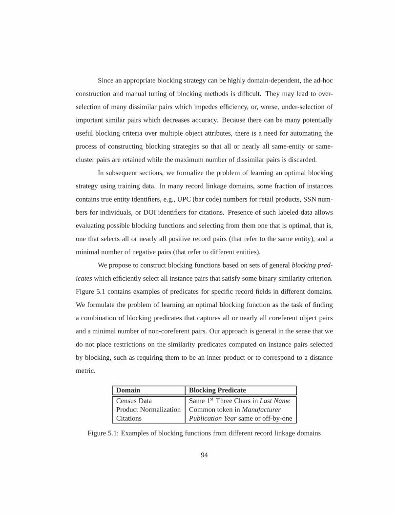
Since an appropriate blocking strategy can be highly domain-dependent, the ad-hoc
construction and manual tuning of blocking methods is difficult. They may lead to over-
selection of many dissimilar pairs which impedes efficiency, or, worse, under-selection of
important similar pairs which decreases accuracy. Becausethere can be many potentially
useful blocking criteria over multiple object attributes,there is a need for automating the
process of constructing blocking strategies so that all or nearly all same-entity or same-
cluster pairs are retained while the maximum number of dissimilar pairs is discarded.
In subsequent sections, we formalize the problem of learning an optimal blocking
strategy using training data. In many record linkage domains, some fraction of instances
contains true entity identifiers, e.g., UPC (bar code) numbers for retail products, SSN num-
bers for individuals, or DOI identifiers for citations. Presence of such labeled data allows
evaluating possible blocking functions and selecting fromthem one that is optimal, that is,
one that selects all or nearly all positive record pairs (that refer to the same entity), and a
minimal number of negative pairs (that refer to different entities).
We propose to construct blocking functions based on sets of generalblocking pred-
icateswhich efficiently select all instance pairs that satisfy some binary similarity criterion.
Figure 5.1 contains examples of predicates for specific record fields in different domains.
We formulate the problem of learning an optimal blocking function as the task of finding
a combination of blocking predicates that captures all or nearly all coreferent object pairs
and a minimal number of non-coreferent pairs. Our approach is general in the sense that we
do not place restrictions on the similarity predicates computed on instance pairs selected
by blocking, such as requiring them to be an inner product or to correspond to a distance
metric.
Domain Blocking Predicate
Census Data Same 1st Three Chars inLast NameProduct Normalization Common token inManufacturerCitations Publication Yearsame or off-by-one
Figure 5.1: Examples of blocking functions from different record linkage domains
94
We consider two types of blocking functions: (1) disjunctions of blocking pred-
icates, and (2) predicates combined in disjunctive normal form (DNF). While finding a
globally optimal solution for these formulations is NP-hard, we describe an effective ap-
proximation method for them and discuss implementation issues. Empirical evaluation on
synthetic and real-world record linkage datasets demonstrates the efficiency of our tech-
niques.
5.2 Adaptive Blocking Formulation
Let us formally define the problem of learning an optimal blocking function. We assume
that a training datasetDtrain = fX ;Y g is available that includes a setX = fxigni=1 of n
records known to refer tom true objects:Y = fyigni=1, where eachyi is the true object
identifier for thei-th record:yi 2 f1; : : : ;mg. Each recordxi may have one or more fields.
We assume that a set ofs generalblocking predicatesfpigsi=1 is available, where
each predicatepi corresponds to two functions:� Indexing function hi(�) is a unary function that is applied to a field value from some
domain Dom(hi) (e.g., strings, integers, or categories) and generates oneor morekeys
for the field value:hi : Dom(hi)! U�, whereU is the set of all possible keys;� Equality function pi(�; �) returns 1 if the intersection of the key sets produced by
the indexing function on its arguments is non-empty, and returns zero otherwise:
pi(x j ;xk) = 1 iff hi(x j)\ hi(xk) 6= /0. Any pair (x j ;xk) for which pi(x j ;xk) = 1 is
coveredby the predicatepi .
Each general blocking predicate can be instantiated for a particular field (or a com-
bination of fields) in a given domain, resulting in severalspecificblocking predicates for the
domain. Given a database withd fields and a set ofsgeneral blocking predicates, we obtain
t � s�d specific predicatesP = fpigti=1 by applying the general predicates to all fields of
95

Sample record:
author
Freund, Y.year
(1995).title
Boosting a weak learning algorithm by majority.venue
Information and Computation,other
121(2), 256-285
Blocking predicates and key sets produced by their indexingfunctions for the record:
author title venue year other
ContainCommonToken
ffreund, yg fboosting,a, weak,learning,algorithm,by,majorityg finformation,
computationg f1995g f121, 2, 256, 285gExact Match f’freund y’g f’boosting a
weaklearningalgorithm bymajority’g f’information
andcomputation’g f’1995’g f’121 2 256 285’g
Same 1st
Three Charsffreg fboog finfg f199g f121g
ContainsSame orOff-By-OneInteger
/0 /0 /0 f19941995,19951996g f120 121, 121122,
1 2, 2 3, 255256,256 257, 284285,285 286g
Figure 5.2: Blocking key values for a sample record
the appropriate type. For example, suppose we have four general predicates defined for all
textual fields:“Contain Common Token”, “Exact Match”, and“Same1st Three Chars”,
“Contains Same of Off-By-One Integer”. When these general predicates are instantiated
for the bibliographic citation domain with five textual fields, author, title, venue, year, and
other, we obtain 5�4= 20 specific blocking predicates for this domain. Figure 5.2 demon-
strates the values produced by the indexing functions of these specific blocking predicates
on a sample citation record (we assume that all strings are converted to lower-case and
punctuation is removed before the application of the indexing functions):
Multiple blocking predicates are combined by an overallblocking function fP con-
structed using the setP of predicates. Like the individual predicates,fP corresponds to an
96
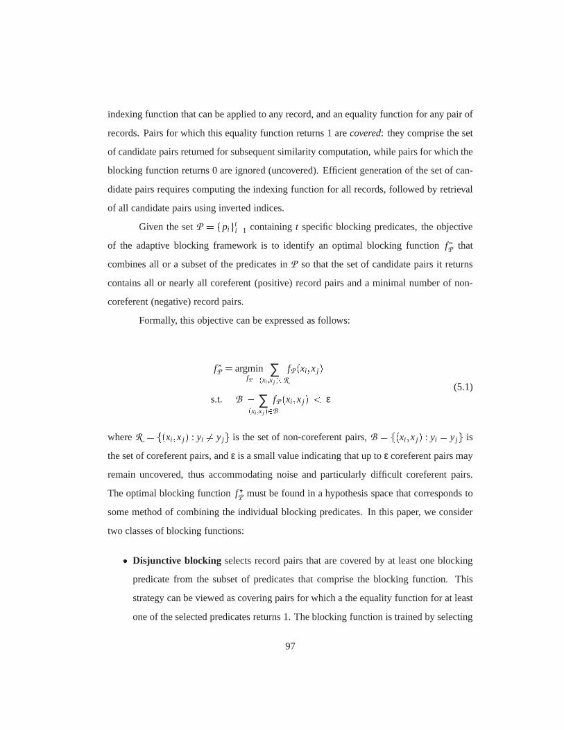
indexing function that can be applied to any record, and an equality function for any pair of
records. Pairs for which this equality function returns 1 are covered: they comprise the set
of candidate pairs returned for subsequent similarity computation, while pairs for which the
blocking function returns 0 are ignored (uncovered). Efficient generation of the set of can-
didate pairs requires computing the indexing function for all records, followed by retrieval
of all candidate pairs using inverted indices.
Given the setP = fpigti=1 containingt specific blocking predicates, the objective
of the adaptive blocking framework is to identify an optimalblocking function f �P that
combines all or a subset of the predicates inP so that the set of candidate pairs it returns
contains all or nearly all coreferent (positive) record pairs and a minimal number of non-
coreferent (negative) record pairs.
Formally, this objective can be expressed as follows:
f �P = argminfP
∑(xi ;xj )2R
fP (xi ;x j)s.t. jB j� ∑(xi ;xj )2B
fP (xi ;x j) < ε(5.1)
whereR = f(xi ;x j) : yi 6= y jg is the set of non-coreferent pairs,B = f(xi ;x j) : yi = y jg is
the set of coreferent pairs, andε is a small value indicating that up toε coreferent pairs may
remain uncovered, thus accommodating noise and particularly difficult coreferent pairs.
The optimal blocking functionf �P must be found in a hypothesis space that corresponds to
some method of combining the individual blocking predicates. In this paper, we consider
two classes of blocking functions:� Disjunctive blocking selects record pairs that are covered by at least one blocking
predicate from the subset of predicates that comprise the blocking function. This
strategy can be viewed as covering pairs for which a the equality function for at least
one of the selected predicates returns 1. The blocking function is trained by selecting
97
a subset of blocking predicates fromP .� Disjunctive Normal Form (DNF) blocking selects object pairs that are covered by
at least one conjunction of blocking predicates from a constructed set of conjunctions.
This strategy can be viewed as covering record pairs for which at least one equality
function of a conjunction of predicates returns 1. The blocking function is trained by
constructing a DNF formula from the blocking predicates.
Each type of blocking functions leads to a distinct formulation of the objective (5.1),
and we consider them individually in the following subsections.
5.2.1 Disjunctive blocking
Given a set of specific blocking predicatesP = fpigti=1, a disjunctive blocking function
corresponds to selecting some subset of predicatesP 0 � P , performing blocking using
eachpi 2 P 0, and then selecting record pairs that share at least one common key in the
key sets computed by the indexing functions of the selected predicates. Thus, the equality
function for the disjunctive blocking function based on subsetP 0 = fpi1; : : : ; pikg of pred-
icates returns 1 if the equality function for at least one predicate returns 1:fP 0(xi ;x j) =[pi1(xi ;x j)+ � � �+ pik(xi ;x j)℄ where[π℄ = 1 if π > 0, and 0 otherwise. If the equality func-
tion for the overall blocking functionfP 0 returns 1 for a pair(xi ;x j), we say that this pair is
coveredby the blocking function.
Learning the optimal blocking functionf �P requires selecting a subsetP � of predi-
cates that results in all or nearly all coreferent pairs being covered by at least one predicate
in P �, and a minimal number of non-coreferent pairs being covered. Then the general
adaptive blocking problem in Eq.(5.1) can be written as follows:
98
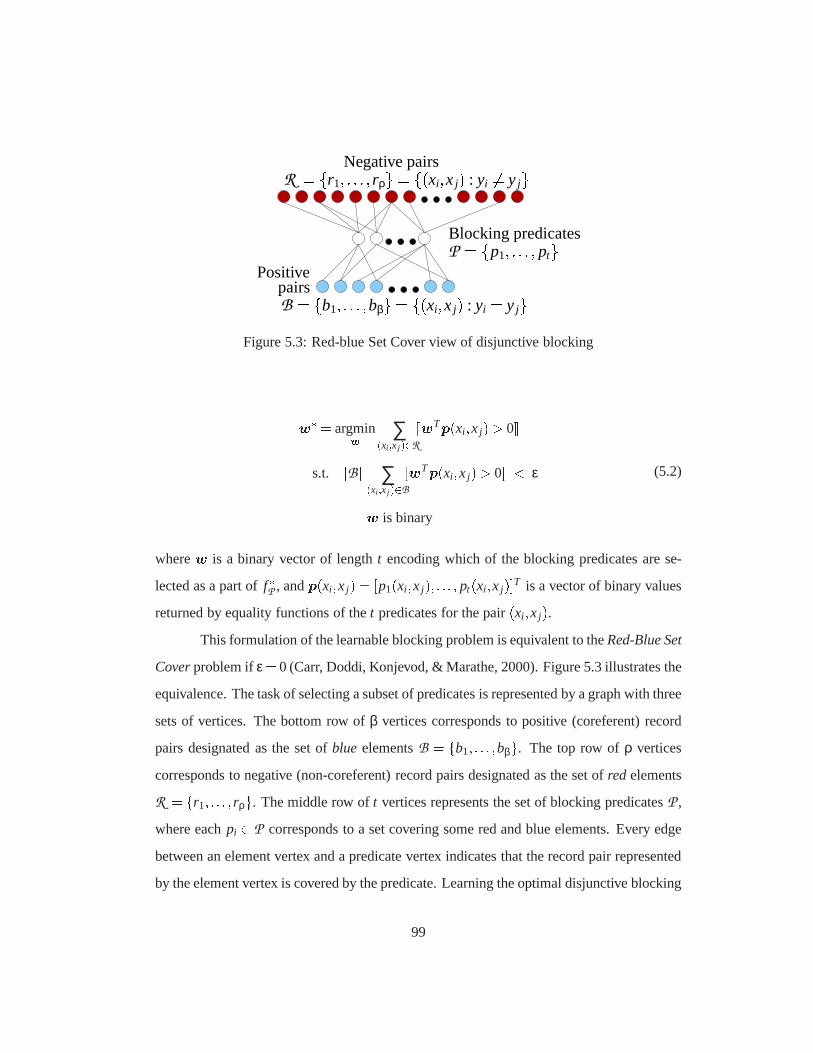
Positive
Negative pairs
pairs
Blocking predicatesP = fp1; : : : ; ptg
R = fr1; : : : ; rρg= f(xi;x j) : yi 6= y jg
B = fb1; : : : ;bβg= f(xi;x j) : yi = y jgFigure 5.3: Red-blue Set Cover view of disjunctive blocking
w� = argminw ∑(xi ;xj )2R
[wTp(xi ;x j)> 0℄s.t. jB j� ∑(xi ;xj )2B
[wTp(xi ;x j)> 0℄ < εw is binary
(5.2)
wherew is a binary vector of lengtht encoding which of the blocking predicates are se-
lected as a part off �P , andp(xi;x j) = [p1(xi ;x j); : : : ; pt(xi ;x j)℄T is a vector of binary values
returned by equality functions of thet predicates for the pair(xi ;x j).This formulation of the learnable blocking problem is equivalent to theRed-Blue Set
Coverproblem ifε= 0 (Carr, Doddi, Konjevod, & Marathe, 2000). Figure 5.3 illustrates the
equivalence. The task of selecting a subset of predicates isrepresented by a graph with three
sets of vertices. The bottom row ofβ vertices corresponds to positive (coreferent) record
pairs designated as the set ofblue elementsB = fb1; : : : ;bβg. The top row ofρ vertices
corresponds to negative (non-coreferent) record pairs designated as the set ofred elements
R = fr1; : : : ; rρg. The middle row oft vertices represents the set of blocking predicatesP ,
where eachpi 2 P corresponds to a set covering some red and blue elements. Every edge
between an element vertex and a predicate vertex indicates that the record pair represented
by the element vertex is covered by the predicate. Learning the optimal disjunctive blocking
99
function is then equivalent to selecting a subset of predicate vertices with their incident
edges so that at leastβ� ε blue (positive) vertices have at least one incident edge, while the
cover cost, equal to the number of red (negative) vertices with at leastone incident edge, is
minimized.
5.2.2 DNF Blocking
In some domains, a disjunctive combination of blocking predicates may be an insufficient
representation of the optimal blocking strategy. For example, in US Census data, conjunc-
tions of predicates such as“Same Zipcode AND Same1st Char in Surname”yield useful
blocking criteria (Winkler, 2005). To incorporate such blocking criteria, we must extend the
disjunctive formulation described above to a formulation based on combining predicates in
disjunctive normal form (DNF). Then, the hypothesis space for the blocking function must
include disjunctions of not just individual blocking predicates, but also of their conjunc-
tions.
A search for the optimal DNF blocking function can be viewed as solving an ex-
tended variant of the red-blue set cover problem. In that variant, the cover is constructed
using not only the sets representing the original predicates, but also using additionally
constructed sets representing predicate conjunctions. Because the number of all possible
conjunctions is exponential, only conjunctions up to fixed lengthk are considered. In Fig-
ure 5.3, considering a conjunction of blocking predicates corresponds to adding a vertex to
the middle row, with edges connecting it to the red and blue vertices present in the intersec-
tion of covered vertex sets for the individual predicates inthe conjunction.
The learnable blocking problem based on DNF blocking functions is then equiv-
alent to constructing a set of conjunctions followed by selection of a set of predicate and
conjunction vertices so that at leastβ� ε positive (blue) vertices have at least one incident
edge, while the cost, equal to the number of negative (red) nodes with at least one incident
edge, is minimized.
100
5.3 Algorithms
5.3.1 Pairwise Training Data
For clustering settings, supervision corresponds to sets of must-link (same-cluster) and
cannot-link (different-cluster) pairs. For record linkage, supervision is available in many
domains in the form of records for which the true entities to which they refer are known,
as discussed in Section 5.1. Such labeled records comprise the training datasetDtrain =fX ;Y g that can be used to generate the pairwise supervision for learning the blocking
function in the form of coreferent (positive) and non-coreferent (negative) record pairs. For
large databases, it is impractical to explicitly generate and store in memory all positive pairs
and negative pairs. However, the set of covered pairs for each predicate can be computed
using the indexing function of the predicate to form an inverted index based on the key
values returned by the indexing function. Then, bit arrays can be used to store the cover of
each predicate, obtained by iteration over the inverted index.
If training data is unavailable, it can be obtained automatically by performing link-
age or clustering without blocking, and then using the linkage or clustering results as train-
ing data for learning a blocking function for the given domain.
5.3.2 Learning Blocking Functions
Disjunctive Blocking
The equivalence of learning optimal disjunctive blocking and the red-blue set cover problem
described in Section 5.2.1 has discouraging implications for the practitioner. The red-blue
set cover problem is NP-hard, and Carr et al. (2000) have shown that unless P=NP, it cannot
be efficiently approximated within a factorO(2log1�δ t);δ = 1=log logc t, wheret is the num-
ber of predicates under consideration. On the other hand, several approximate algorithms
have been proposed for the red-blue set cover problem (Carr et al., 2000; Peleg, 2000). We
base our approach on a modified version of Peleg’s greedy algorithm that has an approxi-
101
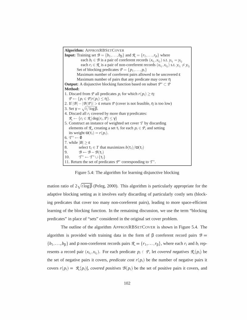
Algorithm: APPROXRBSETCOVER
Input: Training setB = {b1, . . . ,bβ} andR = {r1, . . . , rρ} whereeachbi ∈ B is a pair of coreferent records(xi1,xi2) s.t. yi1 = yi2eachr i ∈ R is a pair ofnon-coreferent records(xi1,xi2) s.t. yi1 6= yi2
Set of blocking predicatesP = {p1, . . . , pt}Maximum number of coreferent pairs allowed to be uncoveredεMaximum number of pairs that any predicate may coverη
Output: A disjunctive blocking function based on subsetP ∗ ⊂ P
Method:1. Discard fromP all predicatespi for which r(pi) ≥ η:
P ←{pi ∈ P |r(pi) ≤ η}.2. If |B |− |B(P )| > ε returnP (cover is not feasible,η is too low)3. Setγ =
√
t/ logβ.4. Discard allr i covered by more thanγ predicates:
R ←{r i ∈ R |deg(r i ,P ) ≤ γ}5. Construct an instance of weighted set coverT by discarding
elements ofR , creating a setτi for eachpi ∈ P , and settingits weightω(τi) = r(pi).
6. T ∗ ← /07. while |B| ≥ ε8. selectτi ∈ T that maximizesb(τi)/ω(τi)9. B ← B −B(τi)10. T ∗ ← T ∗∪{τi}11. Return the set of predicatesP ∗ corresponding toT ∗.
Figure 5.4: The algorithm for learning disjunctive blocking
mation ratio of 2p
t logβ (Peleg, 2000). This algorithm is particularly appropriatefor the
adaptive blocking setting as it involves early discarding of particularly costly sets (block-
ing predicates that cover too many non-coreferent pairs), leading to more space-efficient
learning of the blocking function. In the remaining discussion, we use the term “blocking
predicates” in place of “sets” considered in the original set cover problem.
The outline of the algorithm APPROXRBSETCOVER is shown in Figure 5.4. The
algorithm is provided with training data in the form ofβ coreferent record pairsB =fb1; : : : ;bβg andρ non-coreferent records pairsR = fr1; : : : ; rβg, where eachr i andbi rep-
resents a record pair(xi1;xi2). For each predicatepi 2 P , let covered negativesR (pi) be
the set of negative pairs it covers,predicate cost r(pi) be the number of negative pairs it
coversr(pi) = jR (pi)j, covered positivesB(pi) be the set of positive pairs it covers, and
102
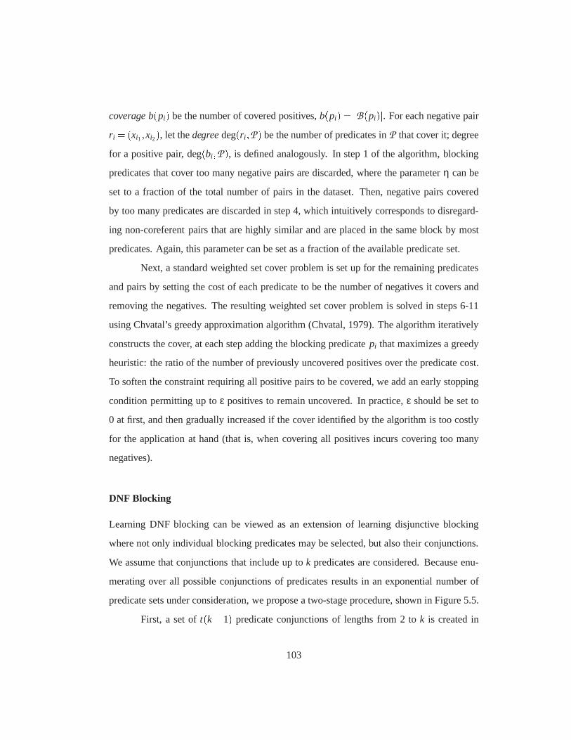
coverage b(pi) be the number of covered positives,b(pi) = jB(pi)j. For each negative pair
r i = (xi1;xi2), let thedegreedeg(r i ;P ) be the number of predicates inP that cover it; degree
for a positive pair, deg(bi ;P ), is defined analogously. In step 1 of the algorithm, blocking
predicates that cover too many negative pairs are discarded, where the parameterη can be
set to a fraction of the total number of pairs in the dataset. Then, negative pairs covered
by too many predicates are discarded in step 4, which intuitively corresponds to disregard-
ing non-coreferent pairs that are highly similar and are placed in the same block by most
predicates. Again, this parameter can be set as a fraction ofthe available predicate set.
Next, a standard weighted set cover problem is set up for the remaining predicates
and pairs by setting the cost of each predicate to be the number of negatives it covers and
removing the negatives. The resulting weighted set cover problem is solved in steps 6-11
using Chvatal’s greedy approximation algorithm (Chvatal,1979). The algorithm iteratively
constructs the cover, at each step adding the blocking predicatepi that maximizes a greedy
heuristic: the ratio of the number of previously uncovered positives over the predicate cost.
To soften the constraint requiring all positive pairs to be covered, we add an early stopping
condition permitting up toε positives to remain uncovered. In practice,ε should be set to
0 at first, and then gradually increased if the cover identified by the algorithm is too costly
for the application at hand (that is, when covering all positives incurs covering too many
negatives).
DNF Blocking
Learning DNF blocking can be viewed as an extension of learning disjunctive blocking
where not only individual blocking predicates may be selected, but also their conjunctions.
We assume that conjunctions that include up tok predicates are considered. Because enu-
merating over all possible conjunctions of predicates results in an exponential number of
predicate sets under consideration, we propose a two-stageprocedure, shown in Figure 5.5.
First, a set oft(k�1) predicate conjunctions of lengths from 2 tok is created in
103
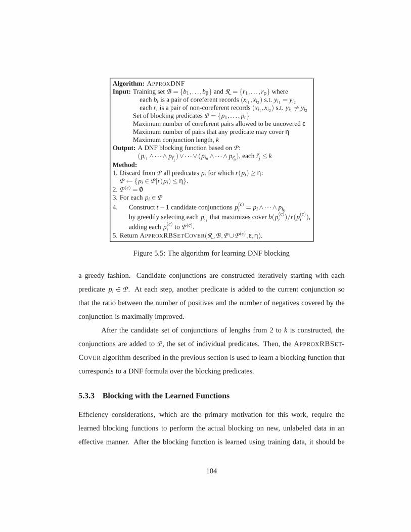
Algorithm: APPROXDNFInput: Training setB = {b1, . . . ,bβ} andR = {r1, . . . , rρ} where
eachbi is a pair of coreferent records(xi1,xi2) s.t. yi1 = yi2eachr i is a pair ofnon-coreferent records(xi1,xi2) s.t. yi1 6= yi2
Set of blocking predicatesP = {p1, . . . , pt}Maximum number of coreferent pairs allowed to be uncoveredεMaximum number of pairs that any predicate may coverηMaximum conjunction length,k
Output: A DNF blocking function based onP :(pi1 ∧·· ·∧ pi′1
)∨·· ·∨ (pin ∧·· ·∧ pi′n), eachi′j ≤ kMethod:1. Discard fromP all predicatespi for which r(pi) ≥ η:
P ←{pi ∈ P |r(pi) ≤ η}.2. P (c) = /03. For eachpi ∈ P
4. Constructt −1 candidate conjunctionsp(c)i = pi ∧·· ·∧ pik
by greedily selecting eachpi j that maximizes coverb(p(c)i )/r(p(c)
i ),
adding eachp(c)i to P (c).
5. Return APPROXRBSETCOVER(R ,B ,P ∪P (c),ε,η).
Figure 5.5: The algorithm for learning DNF blocking
a greedy fashion. Candidate conjunctions are constructed iteratively starting with each
predicatepi 2 P . At each step, another predicate is added to the current conjunction so
that the ratio between the number of positives and the numberof negatives covered by the
conjunction is maximally improved.
After the candidate set of conjunctions of lengths from 2 tok is constructed, the
conjunctions are added toP , the set of individual predicates. Then, the APPROXRBSET-
COVER algorithm described in the previous section is used to learna blocking function that
corresponds to a DNF formula over the blocking predicates.
5.3.3 Blocking with the Learned Functions
Efficiency considerations, which are the primary motivation for this work, require the
learned blocking functions to perform the actual blocking on new, unlabeled data in an
effective manner. After the blocking function is learned using training data, it should be
104
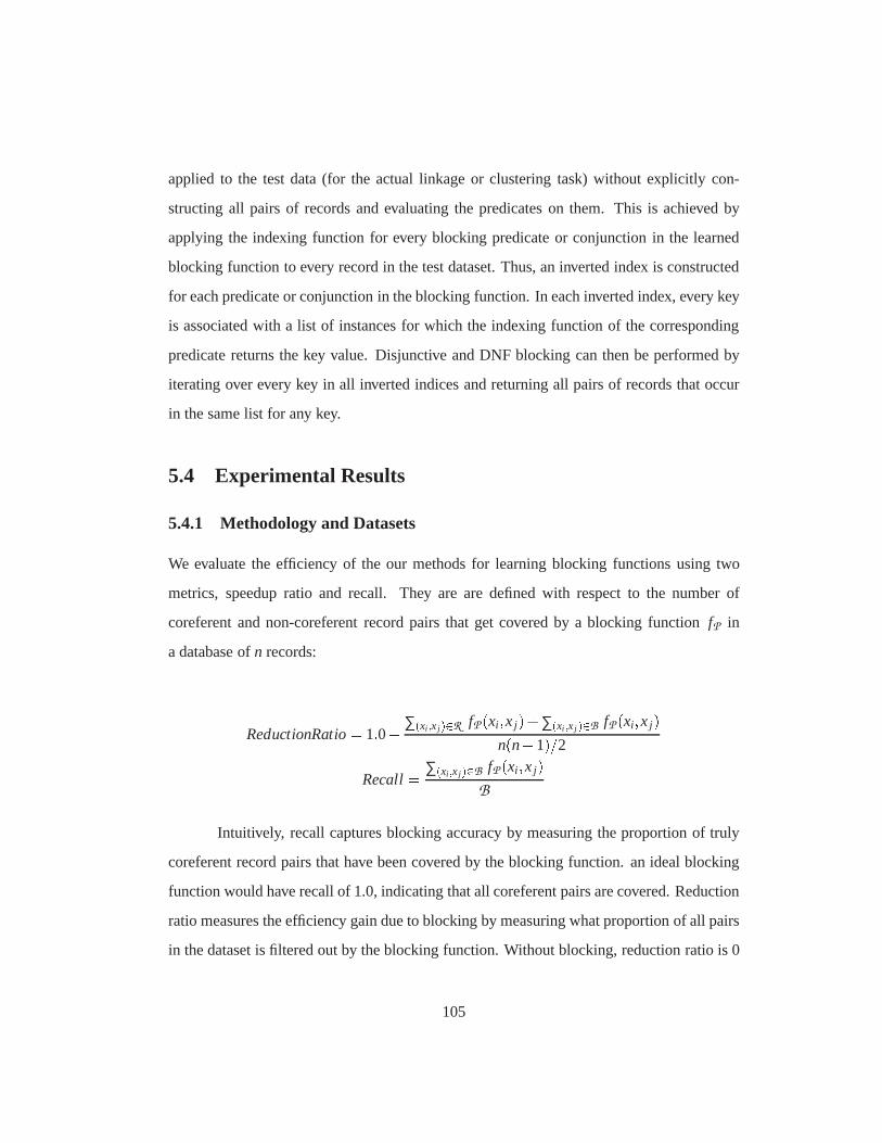
applied to the test data (for the actual linkage or clustering task) without explicitly con-
structing all pairs of records and evaluating the predicates on them. This is achieved by
applying the indexing function for every blocking predicate or conjunction in the learned
blocking function to every record in the test dataset. Thus,an inverted index is constructed
for each predicate or conjunction in the blocking function.In each inverted index, every key
is associated with a list of instances for which the indexingfunction of the corresponding
predicate returns the key value. Disjunctive and DNF blocking can then be performed by
iterating over every key in all inverted indices and returning all pairs of records that occur
in the same list for any key.
5.4 Experimental Results
5.4.1 Methodology and Datasets
We evaluate the efficiency of the our methods for learning blocking functions using two
metrics, speedup ratio and recall. They are are defined with respect to the number of
coreferent and non-coreferent record pairs that get covered by a blocking functionfP in
a database ofn records:
ReductionRatio= 1:0� ∑(xi ;xj )2R fP (xi ;x j)+∑(xi ;xj )2B fP (xi ;x j)n(n�1)=2
Recall= ∑(xi ;xj )2B fP (xi ;x j)jB jIntuitively, recall captures blocking accuracy by measuring the proportion of truly
coreferent record pairs that have been covered by the blocking function. an ideal blocking
function would have recall of 1.0, indicating that all coreferent pairs are covered. Reduction
ratio measures the efficiency gain due to blocking by measuring what proportion of all pairs
in the dataset is filtered out by the blocking function. Without blocking, reduction ratio is 0
105

since all record pairs are returned, while a higher number indicates what proportion of pairs
is not covered, and therefore will not require similarity computations in the subsequent
record linkage stages or in the clustering algorithm. Note that efficiency savings due to
blocking are more substantial if collective (graph-based)inference methods are used for
linkage or clustering (Pasula et al., 2003; McCallum & Wellner, 2004a; Singla & Domingos,
2005; Bhattacharya & Getoor, 2006), as the time complexity of these methods increases
superlinearly with the number of record pairs under consideration.
Results are obtained using 10 runs of two-fold cross-validation. Using a higher
number of folds would result in fewer coreferent records in the test fold, which would
artificially make the blocking task easier. During each run,the dataset is split into two
folds by randomly assigning all records for every underlying entity to one of the folds. The
blocking function is then trained using record pairs generated from the training fold. The
learned blocking function is used to perform blocking on thetest fold, based on which recall
and reduction ratio are measured.
We present results on two datasets:Cora andAddresses. TheCora dataset is de-
scribed in Section 3.1.1. While it is a relatively small-scale dataset, results of Chapter 3
illustrate that good linkage performance on this domain requires computationally intensive
string similarity functions; it has also been shown that linkage on that dataset benefits from
collective linkage methods (Singla & Domingos, 2005), justifying the need for blocking.
Addressesis a dataset containing names and addresses of 50,000 9-fieldrecords for 10,000
unique individuals that was generated using the DBGEN program provided by Hernandez
and Stolfo (1995).
We use the following general predicates are for constructing learnable blocking
functions:� Exact Match: covers instances that have the same value for the field;� Contain Common Token: covers instances that contain a common token in the field
value;
106
� Contain Common Integer: covers instances that contain a common token consisting
of digits in the field value;� Contain Same or Off-by-One Integer: covers instances that contain integer tokens
that are equal or differ by at most 1;� Same N First Chars, N=3;5;7: covers instances that have a common character prefix
in the field value;� Contain Common Token N-gram, N= 2;4;6: covers instances that contain a common
length-N subsequence of tokens;� Token-based TF-IDF> δ; δ = 0:2;0:4;0:6;0:8;1:0: covers instances where token-
based TF-IDF cosine similarity between field values is greater than the thresholdδ;� N-gram-based TF-IDF> δ; δ = 0:2;0:4;0:6;0:8;1:0; N = 3;5: covers instances
where TF-IDF cosine similarity between n-gram representations of field values is
greater than the thresholdδ.
As described in Section 5.2, these general predicates are instantiated for all fields
in the given database. Algorithms presented in Section 5.3.2 are used to construct blocking
functions by selecting subsets of the resulting field-specific predicates. For DNF blocking,
conjunctions of length 2 were employed, as experiments withlonger conjunctions did not
lead to improvements over blocking based on a 2-DNF.
We vary the value of parameterε (which specifies the number of coreferent pairs
allowed to remain uncovered) by setting torβ for different values of desired recallr between
0.0 and 1.0, whereβ is the number of coreferent record pairs in the training fold. This
parameter captures the dependence between the reduction ratio and recall: ifε is high, fewer
predicates are selected resulting in lower recall since notall coreferent pairs are retrieved.
At the same time, the reduction ratio is higher for higherε since fewer pairs are covered by
the learned blocking function, leading to higher efficiency. By varyingε, we obtain a series
107
of results that demonstrate the trade-off between obtaining higher recall and improving the
reduction ratio.
We compare the proposed methods with CANOPIES (McCallum et al., 2000), a
popular blocking method relying on token-based or n-gram-based TF-IDF similarity com-
puted using an inverted index. In a previous study, Baxteret al. (Baxter et al., 2003) have
compared several manually-tuned blocking strategies and found CANOPIES to produce best
overall results. CANOPIESalso allows trading off precision and the reduction ratio byvary-
ing the threshold parameter that controls the coverage of the blocking.1 We tried both
token-based CANOPIESand tri-gram based CANOPIESand chose the best-performing vari-
ants as baselines: token-based indexing forCora, and tri-gram indexing forAddresses. This
difference is due to the fact that most variation between coreferent citations inCora is due
to insertions and deletions of whole words, making token-based similarity more appropri-
ate. Coreferent records inAddresses, on other hand, mostly differ due to misspellings and
character-level transformations that n-gram similarity is able to capture.
5.4.2 Results and Discussion
Figures 5.6 and 5.7 show the reduction ratio versus recall curves for the two types of learned
blocking functions described above and for CANOPIES. From these results, we observe that
both variants of adaptive blocking outperform the unlearned baseline: combining multiple
predicates allows achieving higher recall levels as well asachieving higher reduction ratios.
DNF blocking is more accurate than disjunctive blocking, and onAddressesit also achieves
higher recall, while forCora the maximum recall is comparable. Because DNF blocking
is based on predicate conjunctions, non-coreferent pairs are easier avoided by the blocking
function: conjunctions effectively form high-precision,low-recall rules that cover smaller
subsets of coreferent pairs but fewer non-coreferent pairscompared to single predicates.
1The original CANOPIESalgorithm allows varying two separate threshold parameters, however, empiricalresults have shown that using the same value for both thresholds yields highest performance (McCallum et al.,2000).
108
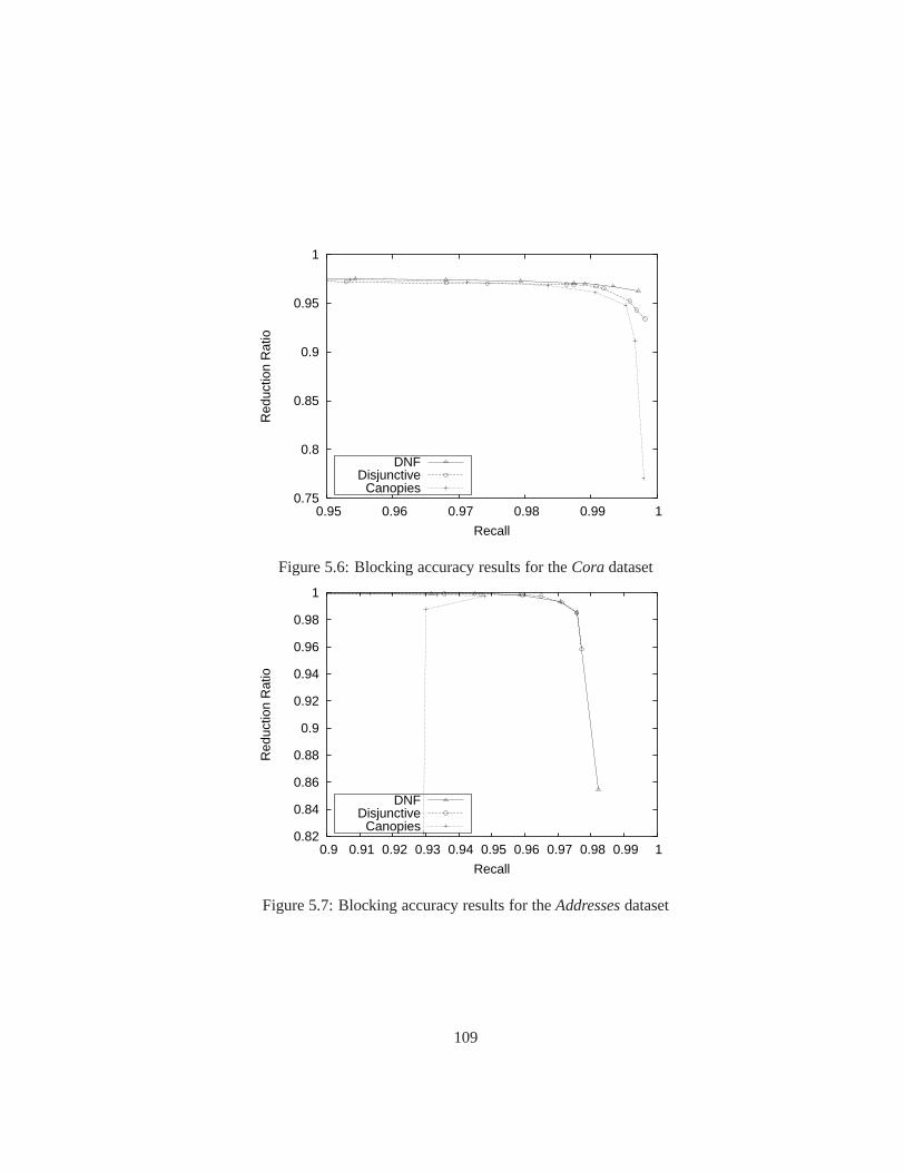
0.75
0.8
0.85
0.9
0.95
1
0.95 0.96 0.97 0.98 0.99 1
Red
uctio
n R
atio
Recall
DNFDisjunctive
Canopies
Figure 5.6: Blocking accuracy results for theCoradataset
0.82
0.84
0.86
0.88
0.9
0.92
0.94
0.96
0.98
1
0.9 0.91 0.92 0.93 0.94 0.95 0.96 0.97 0.98 0.99 1
Red
uctio
n R
atio
Recall
DNFDisjunctive
Canopies
Figure 5.7: Blocking accuracy results for theAddressesdataset
109
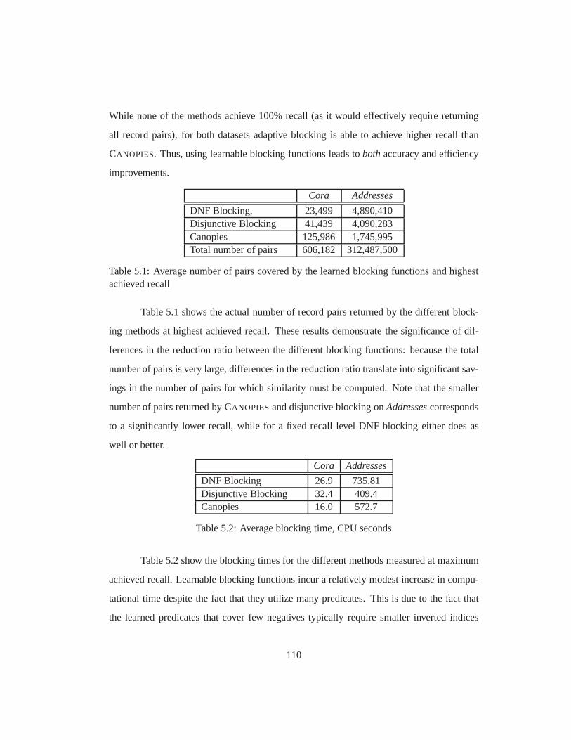
While none of the methods achieve 100% recall (as it would effectively require returning
all record pairs), for both datasets adaptive blocking is able to achieve higher recall than
CANOPIES. Thus, using learnable blocking functions leads tobothaccuracy and efficiency
improvements.
Cora Addresses
DNF Blocking, 23,499 4,890,410Disjunctive Blocking 41,439 4,090,283Canopies 125,986 1,745,995Total number of pairs 606,182 312,487,500
Table 5.1: Average number of pairs covered by the learned blocking functions and highestachieved recall
Table 5.1 shows the actual number of record pairs returned bythe different block-
ing methods at highest achieved recall. These results demonstrate the significance of dif-
ferences in the reduction ratio between the different blocking functions: because the total
number of pairs is very large, differences in the reduction ratio translate into significant sav-
ings in the number of pairs for which similarity must be computed. Note that the smaller
number of pairs returned by CANOPIESand disjunctive blocking onAddressescorresponds
to a significantly lower recall, while for a fixed recall levelDNF blocking either does as
well or better.
Cora Addresses
DNF Blocking 26.9 735.81Disjunctive Blocking 32.4 409.4Canopies 16.0 572.7
Table 5.2: Average blocking time, CPU seconds
Table 5.2 show the blocking times for the different methods measured at maximum
achieved recall. Learnable blocking functions incur a relatively modest increase in compu-
tational time despite the fact that they utilize many predicates. This is due to the fact that
the learned predicates that cover few negatives typically require smaller inverted indices
110
than the one built by canopies using tokens or n-grams where each token or n-gram occurs
in many strings. Many predicates employed by the adaptive blocking functions, on other
hand, map each string to a single key, resulting in more efficient retrieval of covered pairs.
Inverted indices corresponding to conjunctions are even more efficient as they contain many
keys (the cross product of the key sets for the predicates in the conjunction) and incur less
chaining, which is the reason for better performance of DNF blocking compared to disjunc-
tive blocking onCora, where the number of predicates in the constructed blockingfunction
is similar for the two methods. OnAddresses, DNF blocking constructs blocking functions
containing more predicates, which on one hand incurs a computational penalty, but on other
allows it to achieve higher recall.
Overall, the results demonstrate that adaptive blocking functions significantly im-
prove the efficiency of record linkage, and provide an attractive methodology for scaling up
data mining tasks that rely on similarity computations between pairs of instances.
5.5 Related Work
A number of blocking methods have been proposed by researchers for speeding up record
linkage and clustering (Fellegi & Sunter, 1969; Kelley, 1985; Newcombe, 1988; Jaro, 1989;
Hernandez & Stolfo, 1995; McCallum et al., 2000; Baxter et al., 2003; Chaudhuri et al.,
2003; Jin et al., 2003; Gu & Baxter, 2004; Winkler, 2005); seethe summary of these
methods in Section 2.4. A key distinction between prior workand our approach is that
previously described methods focus on improving blocking efficiency while assuming that
an accurate blocking function is known and its parameters have been tuned manually. In
contrast, our approach attempts to construct an optimal blocking function automatically.
Because blocking functions can be learned using any combination of similarity predicates
on different record fields, and no assumptions are made aboutthe number of record fields
or their type, our approach can be used for adapting the blocking function in any domain,
while allowing human experts to add domain-specific predicates.
111
Our predicate-based blocking approach is most closely related to key-based meth-
ods developed by researchers working on record linkage for Census data (Kelley, 1985;
Newcombe, 1988; Jaro, 1989; Winkler, 2005). Techniques described by Kelley (Kelley,
1985) and Winkler (Winkler, 2005) are particularly relevant as they describe methodolo-
gies for evaluating the accuracy of individual blocking predicates, and could be integrated
with our approach for further speedup of blocking function learning.
Our formulation for training disjunctive and DNF blocking functions is related to
machine learning algorithms for learning disjunctive rules and DNFs (Mitchell, 1997). A
principal difference between that work and the learnable blocking problem is that in our
setting the learned disjunctions must cover all positive record pairs while minimizing the
number of covered negative pairs, while rule learning methods generally attempt to equally
minimize the number of errors on both positive and negative examples. Cost-sensitive
machine learning methods (Elkan, 2001) may provide a foundation for other approaches
to adaptive blocking, and we hope that our initial work will encourage the development of
alternative learnable blocking techniques.
5.6 Chapter Summary
In this chapter, we formulated the adaptive blocking problem as the task of learning a func-
tion that returns a minimal number of non-coreferent recordpairs while returning all or
nearly all coreferent pairs. We described two types of blocking functions: disjunctive and
DNF blocking. Formulating the learning problem as an instance of the Red-Blue Set Cover
problem allowed us to adopt a well-known approximation algorithm for that problem to
construct blocking functions. Experimental results demonstrated the ability of our approach
to learn efficient and accurate blocking functions automatically.
112

Chapter 6
Future Work
Because learnable similarity functions are a part of many machine learning and data analy-
sis tasks, there is a large number of applications where adapting distance computations can
have a significant effect on performance. These applications can be found in such fields
as natural language processing, information retrieval, vision, robotics and bioinformatics,
where application-specific similarity functions are oftenemployed. Adapting such func-
tions in situ in these applications can be achieved using the framework used in the three
applications considered in this thesis: learning from pairwise supervision. While specific
applications in the above areas are beyond the scope of this thesis, in subsequent sections
we describe several directions for future work that are directly related to the applications
and similarity functions considered in prior chapters.
6.1 Multi-level String Similarity Functions
Improvements obtained using learnable affine-gap edit distance over its unlearned equiv-
alent demonstrated the benefits of adapting string similarity computations to a given do-
main. However, edit distance has certain properties that may limit its suitability in some
domains. For example, it does not directly handle transpositions of entire fragments (e.g.,
113
token swaps), and while edit operations for short-range transpositions can be added at
considerable computational cost, handling long-term transpositions is problematic. Order-
insensitive similarity functions such as cosine similarity, on other hand, have no trouble
dealing with token transpositions, yet they depend on accurate tokenization and suffer when
edit operations occur at the character level.
The SoftTFIDF variant of cosine similarity recently proposed by Cohen et al. (2003a)
attempts to amend this drawback of cosine similarity, yet itcannot adapt to a given domain
beyond the IDF weighting. An exciting challenge for future work lies in developing learn-
able string similarity functions that integrate adaptive string comparison at the character,
token, and document (string) levels. Such similarity functions must rely on joint similarity
computation across the levels while remaining computationally efficient. While segmented
pair HMMs presented in Section 3.1.2 are a first step in this direction, developing string
similarity models that perform further structural analysis of strings remains an open re-
search issue. Progress in this area will have impact in all tasks that rely on string similarity
functions such as record linkage and information retrieval.
6.2 Discriminative Pair HMMs
The Expectation-Maximization algorithm that we describedin Chapter 3 for training pair
HMMs only utilizes positive supervision: the learning procedure maximizes the likelihood
of observing alignments of coreferent pairs. However, it may be advantageous to exploit
negative supervision, that is, pairs of non-coreferent strings, since some “near-miss” nega-
tive examples can be very informative.
A recently proposed edit distance model based on Conditional Random Fields (CRFs)
has structure that allows training with both positive and negative examples so that the model
directly learns to discriminate between the two kinds of pairs (McCallum et al., 2005). The
CRF edit distance model consists of two three-state edit distance transducers, one of which
computes the alignment probabilities for coreferent strings, while the other computes align-
114
ment probabilities for non-coreferent strings.
Although the CRF-based model has different probabilistic semantics (alignments
are not generated since the model is conditioned on the fact that any two strings under con-
sideration are aligned), the coupled structure of that model can be implemented as a pair
HMM. Considering such coupled structures within the pair HMM framework is an interest-
ing area for future work, since it would allow applying discriminative training methods that
explicitly attempt to learn model parameters that effectively distinguish between coreferent
and non-coreferent strings (Eisner, 2002). Another avenuefor future work on alternative
pair HMM structures involves deriving learnable models forlocal alignment that focus
on scoring matching alignment fragments while disregarding the mismatched sequences
around them (Gusfield, 1997). In domains where large gaps arecommonplace yet small
matching sequences may be very informative, e.g., in linkage of retail product descriptions,
pair HMM structures that model local alignment may yield better performance, and inves-
tigating this possibility is an interesting future direction.
6.3 Active Learning of Similarity Functions
As discussed in Section 3.3, the goal of active learning methods for similarity functions is
identifying pairs of objects whose equivalence or non-equivalence is informative for im-
proving distance estimates. The classifier-based record similarity described in Section 3.2
lends itself nicely to active learning techniques developed for classification, which has been
explored by Sarawagi and Bhamidipaty (2002) and Tejada et al. (2002) in the record linkage
context.
One of the biggest challenges in selecting useful training example pairs lies with
the fact that the space of possible pairs grows quadratically with the number of examples,
and static-active and weakly-labeled methodologies we proposed in Section 3.3 address this
challenge. However, these methods are based on heuristics,while developing more princi-
pled active learning methods remains an interesting direction for future work. Such methods
115
must directly attempt to identify example pairs that would lead to maximal improvement
of similarity estimates. Traditional active learning approaches such as uncertainty sam-
pling (Lewis & Catlett, 1994), query-by-committee (Seung et al., 1992), estimation error
reduction (Lindenbaum et al., 1999; Roy & McCallum, 2001), and version space reduc-
tion (Tong, 2001) could be adopted for this task, and developing such methods for directly
improving the learning of similarity functions like edit distance or distortion measures de-
scribed in Chapter 4 is an area yet to be explored.
6.4 From Adaptive Blocking to Learnable Metric Mapping
The predicate-based methodology that we proposed in Chapter 5 for automatically obtain-
ing accurate blocking functions requires specifying an initial set of blocking predicates.
Although a sufficiently general set of predicates for textual data is easy to encode, in future
work it would be interesting to explore learnable blocking methods that are not predicate-
based but rely on mapping records to metric spaces. Several existing blocking methods rely
on such mapping, such as those of Jin et al. (2003) and Chaudhuri et al. (2003). Learning
algorithms that would make these methods adaptive could pursue two directions: searching
for an optimal mapping of data to metric space, or transforming the metric space after the
mapping to allow efficient yet accurate selection of approximately similar records.
This problem is related to methods for fast nearest-neighbor searching, a number
of which have been developed in the past decade (Indyk & Motwani, 1998; Liu, Moore,
Gray, & Yang, 2004; Beygelzimer, Kakade, & Langford, 2006).However, using these
techniques for domains where data is described by multiple fields of heterogeneous types
is non-trivial as they typically rely on strong metric assumptions on the data space, and do
not scale efficiently to high-dimensional data. Developingadaptive nearest-neighbor search
methods for heterogeneous data is an interesting area for future work that has applications in
blocking as well as in other tasks where retrieving approximately similar objects efficiently
is important, e.g., in classification methods and database retrieval.
116
Chapter 7
Conclusions
Research presented in this thesis has focused on learning similarity functions from pairwise
supervision. We have shown that by parameterizing several popular distance functions and
learning parameter values from examples of similar and dissimilar instance pairs, we obtain
increases in accuracy of similarity computations, which lead to performance improvements
in tasks that rely on them: record linkage, semi-supervisedclustering, and blocking.
First, we have considered learning similarity functions inthe context of record link-
age where they are used for two tasks: computing similarity between individual field values
and combining these similarities across multiple fields. For field-level similarity computa-
tions, we have described two adaptive variants of affine-gapedit distance in which the costs
of string transformations are learned on a corpus of coreferent string pairs. Our approach is
based on pair HMMs, a probabilistic model for generating string alignments. Learning the
costs of affine-gap edit distance parameters allows adapting the underlying string match-
ing algorithm to each field’s domain, while using segmented pair HMMs integrates such
adaptation with performing string segmentation that is helpful in domains where strings are
composed of multiple fields from different domains.
For computing similarity between records in linkage, we have demonstrated that
Support Vector Machines (SVMs) effectively combine similarities from individual fields in
117
proportion to their relative importance. Using learnable similarity functions at both field and
record levels leads to improved results over using record-level learnable similarity functions
that combine unlearned field-level similarities.
We have proposed two strategies for selecting informative pairs of coreferent or
non-coreferent examples for training similarity functions in record linkage. One of the
proposed strategies, weakly-labeled negative selection does not require labeled supervision,
while the other, likely positive pair selection, avoids thecomputational costs of the standard
active learning methods. Both of these strategies facilitate efficient selection of training
pairs that allows learning accurate similarity functions on small training sets.
Second, we have demonstrated the utility of employing learnable similarity func-
tions in semi-supervised clustering. By incorporating similarity function learning within the
HMRF-KMEANS algorithm for semi-supervised clustering, we were able to leverage both
labeled pairwise supervision and unlabeled data when adapting the similarity functions.
Our approach allows learning individual similarity functions for different clusters which is
useful for domains where clusters have different shapes. The proposed framework can be
used with a variety of distortion (distance) functions thatinclude directional measures such
as cosine similarity, and Bregman divergences that includeEuclidean distance and Kull-
back Leibler divergence. Ablation experiments have demonstrated that the HMRF-based
approach combines the strengths of learnable similarity functions and constrained cluster-
ing to obtain significant improvements in clustering quality.
In the context of blocking, the third application we considered, we have proposed
methods for learning similarity functions that efficientlyselect approximately similar pairs
of examples. Because blocking is required for scaling record linkage and many pairwise
clustering algorithms up to large datasets, our technique shows that learnable similarity
functions can be employed not only for increasing accuracy of data mining tasks, but also
for improving their scalability. Unlike previous blockingmethods that require manual tun-
ing and hand-construction of blocking functions, our approach is adaptive as it optimizes
118
the blocking function for a given domain using pairwise supervision that can be naturally
obtained in linkage and clustering tasks.
For the three tasks under consideration, we have evaluated the effectiveness of uti-
lizing learnable similarity functions, comparing their accuracy on standard benchmarks
with that of unlearned similarity functions typically usedin these tasks. Our experiments
demonstrate that learnable similarity functions effectively utilize the pairwise training data
to make distance estimates more accurate for a given domain,resulting in overall perfor-
mance improvements on the tasks.
Overall, the work presented in this thesis contributes methods leading to state-of-
the art performance on the considered tasks and provides a number of useful algorithms
for practitioners in record linkage, semi-supervised clustering, and blocking. This research
demonstrates the power of using similarity functions that can adapt to a given domain using
pairwise supervision, and we hope that it will motivate further research in trainable distance
functions, as well as encourage employing such functions invarious applications where
distance estimates between instances are required.
119

Bibliography
Aha, D. W. (1998). Feature weighting for lazy learning algorithms. In Liu, H., & Motoda,
H. (Eds.),Feature Extraction, Construction and Selection: A Data Mining Perspec-
tive. Kluwer Academic Publishers, Norwell, MA.
Ananthakrishna, R., Chaudhuri, S., & Ganti, V. (2002). Eliminating fuzzy duplicates in
data warehouses. InProceedings of the 28th International Conference on Very Large
Databases (VLDB-2002)Hong Kong, China.
Baeza-Yates, R., & Ribeiro-Neto, B. (1999).Modern Information Retrieval. ACM Press,
New York.
Banerjee, A., Dhillon, I., Ghosh, J., & Sra, S. (2005a). Clustering on the unit hypersphere
using von Mises-Fisher distributions.Journal of Machine Learning Research, 6,
1345–1382.
Banerjee, A., Merugu, S., Dhilon, I., & Ghosh, J. (2005b). Clustering with Bregman diver-
gences.Journal of Machine Learning Research, 6, 1705–1749.
Banerjee, A., Krumpelman, C., Basu, S., Mooney, R. J., & Ghosh, J. (2005c). Model-based
overlapping clustering. InProceedings of the Eleventh ACM SIGKDD International
Conference on Knowledge Discovery and Data Mining (KDD-05).
Bar-Hillel, A., Hertz, T., Shental, N., & Weinshall, D. (2003). Learning distance functions
120
using equivalence relations. InProceedings of 20th International Conference on
Machine Learning (ICML-2003), pp. 11–18.
Basu, S. (2005).Semi-supervised Clustering: Probabilistic Models, Algorithms and Exper-
iments. Ph.D. thesis, University of Texas at Austin.
Basu, S., Banerjee, A., & Mooney, R. J. (2002). Semi-supervised clustering by seeding. In
Proceedings of 19th International Conference on Machine Learning (ICML-2002),
pp. 19–26.
Basu, S., Banerjee, A., & Mooney, R. J. (2004). Active semi-supervision for pairwise
constrained clustering. InProceedings of the 2004 SIAM International Conference
on Data Mining (SDM-04).
Basu, S., Bilenko, M., Banerjee, A., & Mooney, R. J. (2006). Probabilistic semi-supervised
clustering with constraints. In Chapelle, O., Scholkopf,B., & Zien, A. (Eds.),Semi-
Supervised Learning. MIT Press, Cambridge, MA.
Basu, S., Bilenko, M., & Mooney, R. J. (2004). A probabilistic framework for semi-
supervised clustering. InProceedings of the Tenth ACM SIGKDD International Con-
ference on Knowledge Discovery and Data Mining (KDD-2004), pp. 59–68 Seattle,
WA.
Baxter, R., Christen, P., & Churches, T. (2003). A comparison of fast blocking methods
for record linkage. InProceedings of the 2003 ACM SIGKDD Workshop on Data
Cleaning, Record Linkage, and Object Consolidation, pp. 25–27 Washington, DC.
Beygelzimer, A., Kakade, S., & Langford, J. (2006). Cover trees for nearest neighbor. In
Proceedings of 23rd International Conference on Machine Learning (ICML-2006).
Bhattacharya, I., & Getoor, L. (2004). Deduplication and group detection using links. In
Proceedings of the 2004 ACM SIGKDD Workshop on Link Analysisand Group De-
tection.
121
Bhattacharya, I., & Getoor, L. (2006). A latent dirichlet model for unsupervised entity
resolution. In6th SIAM Conference on Data Mining (SDM-2006)Bethesda, MD.
Bilenko, M., Kamath, B., & Mooney, R. J. (2006). Adaptive blocking: Learning to scale up
record linkage. InProceedings of the WWW-2006 Workshop on Information Integra-
tion on the Web.
Bilenko, M., & Basu, S. (2004). A comparison of inference techniques for semi-supervised
clustering with hidden Markov random fields. InProceedings of the ICML-2004
Workshop on Statistical Relational Learning and its Connections to Other Fields
(SRL-2004)Banff, Canada.
Bilenko, M., Basu, S., & Mooney, R. J. (2004). Integrating constraints and metric learning
in semi-supervised clustering. InProceedings of 21st International Conference on
Machine Learning (ICML-2004), pp. 81–88 Banff, Canada.
Bilenko, M., Basu, S., & Sahami, M. (2005). Adaptive productnormalization: Using online
learning for record linkage in comparison shopping. InProceedings of the 5th IEEE
International Conference on Data Mining (ICDM-2005), pp. 58–65.
Bilenko, M., & Mooney, R. J. (2002). Learning to combine trained distance metrics for
duplicate detection in databases. Tech. rep. AI 02-296, Artificial Intelligence Labo-
ratory, University of Texas at Austin, Austin, TX.
Bilenko, M., & Mooney, R. J. (2003a). Adaptive duplicate detection using learnable string
similarity measures. InProceedings of the Ninth ACM SIGKDD International Con-
ference on Knowledge Discovery and Data Mining (KDD-2003), pp. 39–48 Wash-
ington, DC.
Bilenko, M., & Mooney, R. J. (2003b). On evaluation and training-set construction for
duplicate detection. InProceedings of the KDD-03 Workshop on Data Cleaning,
Record Linkage, and Object Consolidation, pp. 7–12 Washington, DC.
122
Blake, C. L., & Merz, C. J. (1998). UCI repository of machine learning databases.
http://www.ics.uci.edu/˜mlearn/MLRepository.html.
Buntine, W. L. (1994). Operations for learning graphical models. Journal of Artificial
Intelligence Research, 2, 159–225.
Carr, R. D., Doddi, S., Konjevod, G., & Marathe, M. (2000). Onthe Red-Blue Set Cover
problem. InProceedings of the 11th Annual ACM-SIAM Symposium on Discrete
Algorithms (SODA-2000)San Francisco, CA.
Chaudhuri, S., Ganjam, K., Ganti, V., & Motwani, R. (2003). Robust and efficient fuzzy
match for online data cleaning. InProceedings of the 2003 ACM SIGMOD Interna-
tional Conference on Management of Data (SIGMOD-03), pp. 313–324. ACM Press.
Chvatal, V. (1979). A greedy heuristic for the set covering problem.Mathematics of Oper-
ations Research, 4(3), 233–235.
Cohen, W. W. (1998). Integration of heterogeneous databases without common domains
using queries based on textual similarity. InProceedings of the 1998 ACM SIGMOD
International Conference on Management of Data (SIGMOD-98), pp. 201–212 Seat-
tle, WA.
Cohen, W. W., Kautz, H., & McAllester, D. (2000). Hardening soft information sources.
In Proceedings of the Sixth International Conference on Knowledge Discovery and
Data Mining (KDD-2000)Boston, MA.
Cohen, W. W., Ravikumar, P., & Fienberg, S. E. (2003a). A comparison of string distance
metrics for name-matching tasks. InProceedings of the IJCAI-2003 Workshop on
Information Integration on the Web, pp. 73–78 Acapulco, Mexico.
Cohen, W. W., Ravikumar, P., & Fienberg, S. E. (2003b). A comparison of string metrics for
matching names and records. InProceedings of the 2003 ACM SIGKDD Workshop on
123
Data Cleaning, Record Linkage, and Object Consolidation, pp. 13–18 Washington,
DC.
Cohen, W. W., & Richman, J. (2002). Learning to match and cluster large high-dimensional
data sets for data integration. InProceedings of the Eighth ACM SIGKDD Inter-
national Conference on Knowledge Discovery and Data Mining(KDD-2002), pp.
475–480 Edmonton, Alberta.
Cohn, D., Caruana, R., & McCallum, A. (2003). Semi-supervised clustering with user
feedback. Tech. rep. TR2003-1892, Cornell University.
Cohn, D. A., Ghahramani, Z., & Jordan, M. I. (1996). Active learning with statistical
models.Journal of Artificial Intelligence Research, 4, 129–145.
Cooper, G. G., & Herskovits, E. (1992). A Bayesian method forthe induction of proba-
bilistic networks from data.Machine Learning, 9, 309–347.
Cover, T. M., & Thomas, J. A. (1991).Elements of Information Theory. Wiley-Interscience.
Dempster, A. P., Laird, N. M., & Rubin, D. B. (1977). Maximum likelihood from incom-
plete data via the EM algorithm.Journal of the Royal Statistical Society B, 39, 1–38.
Dhillon, I. S., & Modha, D. S. (2001). Concept decompositions for large sparse text data
using clustering.Machine Learning, 42, 143–175.
Dhillon, I. S., & Guan, Y. (2003). Information theoretic clustering of sparse co-occurrence
data. InProceedings of the Third IEEE International Conference on Data Mining
(ICDM-2003), pp. 517–521.
Dom, B. E. (2001). An information-theoretic external cluster-validity measure. Research
report RJ 10219, IBM.
124
Dong, X., Halevy, A., & Madhavan, J. (2005). Reference reconciliation in complex infor-
mation spaces. InProceedings of the 2005 ACM SIGMOD international conference
on Management of data (SIGMOD-2005), pp. 85–96 Baltimore, MD.
Duda, R. O., Hart, P. E., & Stork, D. G. (2001).Pattern Classification(Second edition).
Wiley, New York.
Durbin, R., Eddy, S., Krogh, A., & Mitchison, G. (1998).Biological Sequence Analysis:
Probabilistic Models of Proteins and Nucleic Acids. Cambridge University Press.
Eisner, J. (2002). Parameter estimation for probabilisticfinite-state transducers. InProceed-
ings of the 40th Annual Meeting of the Association for Computational Linguistics
(ACL-2002).
Elfeky, M. G., Elmagarmid, A. K., & Verykios, V. S. (2002). TAILOR: A record linkage
tool box. InProceedings of the 18th International Conference on Data Engineering
(ICDE-2002), pp. 17–28.
Elkan, C. (2001). The foundations of cost-sensitive learning. InProceedings of the Seven-
teenth International Joint Conference on Artificial Intelligence (IJCAI-2001).
Fellegi, I. P., & Sunter, A. B. (1969). A theory for record linkage.Journal of the American
Statistical Association, 64(328), 1183–1210.
Fern, X., & Brodley, C. (2003). Random projection for high dimensional data clustering:
A cluster ensemble approach. InProceedings of 20th International Conference on
Machine Learning (ICML-2003).
Freitag, D., & McCallum, A. (1999). Information extractionwith HMMs and shrinkage. In
Papers from the Sixteenth National Conference on ArtificialIntelligence (AAAI-99)
Workshop on Machine Learning for Information Extraction, pp. 31–36 Orlando, FL.
125
Freund, Y., & Schapire, R. E. (1996). Experiments with a new boosting algorithm. InPro-
ceedings of the Thirteenth International Conference on Machine Learning (ICML-
96), pp. 148–156 Bari, Italy. Morgan Kaufmann.
Friedman, J. H. (1997). On bias, variance, 0/1-loss, and thecurse-of-dimensionality.Data
Mining and Knowledge Discovery, 1(1), 55–77.
Geman, S., & Geman, D. (1984). Stochastic relaxation, Gibbsdistributions and the
Bayesian restoration of images.IEEE Transactions on Pattern Analysis and Machine
Intelligence, 6, 721–742.
Giles, C. L., Bollacker, K., & Lawrence, S. (1998). CiteSeer: An automatic citation index-
ing system. InProceedings of the Third ACM Conference on Digital Libraries, pp.
89–98 Pittsburgh, PA.
Golub, G. H., & van Loan, C. F. (1989).Matrix Computations(Second edition). Johns
Hopkins University Press.
Gotoh, O. (1982). An improved algorithm for matching biological sequences.Journal of
Molecular Biology, 162, 705–708.
Grenager, T., Klein, D., & Manning, C. D. (2005). Unsupervised learning of field segmen-
tation models for information extraction. InProceedings of the 43nd Annual Meeting
of the Association for Computational Linguistics (ACL-05).
Gu, L., & Baxter, R. (2004). Adaptive filtering for efficient record linkage. InProceedings
of the Fourth SIAM International Conference on Data Mining (SDM-04).
Gusfield, D. (1997).Algorithms on Strings, Trees and Sequences. Cambridge University
Press, New York.
Hammersley, J., & Clifford, P. (1971). Markov fields on graphs and lattices. Unpublished
manuscript.
126
Hernandez, M. A., & Stolfo, S. J. (1995). The merge/purge problem for large databases. In
Proceedings of the 1995 ACM SIGMOD International Conference on Management
of Data (SIGMOD-95), pp. 127–138 San Jose, CA.
Hofmann, T., & Buhmann, J. M. (1998). Active data clustering. In Advances in Neural
Information Processing Systems 10.
Indyk, P., & Motwani, R. (1998). Approximate nearest neighbors: towards removing the
curse of dimensionality. InProceedings of the 30th ACM Symposium on Theory of
Computing (STOC-98), pp. 604–613.
Jain, A. K., Murty, M. N., & Flynn, P. J. (1999). Data clustering: A review.ACM Computing
Surveys, 31(3), 264–323.
Jaro, M. (1989). Advances in record-linkage methodology asapplied to matching the 1985
census of Tampa, Florida.Journal of the American Statistical Association, 84, 414–
420.
Jelinek, F., & Mercer, R. (1980). Interpolated estimation of markov source parameters from
sparse data. InPattern Recognition in Practice, pp. 381–402.
Jelinek, F. (1998).Statistical Methods for Speech Recognition. MIT Press, Cambridge,
MA.
Jin, L., Li, C., & Mehrotra, S. (2003). Efficient record linkage in large data sets. In
Proceedings of the 8th International Conference on Database Systems for Advanced
Applications (DASFAA-03), pp. 137–148 Kyoto, Japan.
Joachims, T. (2003). Learning to align sequences: A maximum-margin approach. Tech.
rep., Cornell University, Department of Computer Science.
Karypis, G., & Kumar, V. (1998). A fast and high quality multilevel scheme for partitioning
irregular graphs.SIAM Journal on Scientific Computing, 20(1), 359–392.
127
Kaufman, L., & Rousseeuw, P. (1990).Finding Groups in Data: An Introduction to Cluster
Analysis. John Wiley and Sons, New York.
Kearns, M., Mansour, Y., & Ng, A. Y. (1997). An information-theoretic analysis of hard
and soft assignment methods for clustering. InProceedings of 13th Conference on
Uncertainty in Artificial Intelligence (UAI-97), pp. 282–293.
Kelley, R. P. (1985). Advances in record linkage methodology: a method for determining
the best blocking strategy. InRecord Linkage Techniques - 1985: Proceedings of the
Workshop on Exact Matching Methodologies, pp. 199–203 Arlington, VA.
Klein, D., Kamvar, S. D., & Manning, C. (2002). From instance-level constraints to space-
level constraints: Making the most of prior knowledge in data clustering. InPro-
ceedings of 19th International Conference on Machine Learning (ICML-2002), pp.
307–314 Sydney, Australia.
Kschischang, F. R., Frey, B., & Loeliger, H.-A. (2001). Factor graphs and the sum-product
algorithm. IEEE Transactions on Information Theory, 47(2), 498–519.
le Cessie, S., & van Houwelingen, J. C. (1992). Ridge estimators in logistic regression.
Applied Statistics, 41(1), 191–201.
Levenshtein, V. I. (1966). Binary codes capable of correcting insertions and reversals.
Soviet Physics Doklady, 10(8), 707–710.
Lewis, D. D., & Catlett, J. (1994). Heterogeneous uncertainty sampling for supervised
learning. InProceedings of the Eleventh International Conference on Machine Learn-
ing (ICML-94), pp. 148–156 San Francisco, CA. Morgan Kaufmann.
Li, X., Morie, P., & Roth, D. (2004). Identification and tracing of ambiguous names: Dis-
criminative and generative approaches. InProceedings of the 19th National Confer-
ence on Artificial Intelligence (AAAI-2004).
128
Lin, J. (1991). Divergence measures based on the shannon entropy. IEEE Transactions on
Information Theory, 37(1), 145–151.
Lindenbaum, M., Markovitch, S., & Rusakov, D. (1999). Selective sampling for nearest
neighbor classifiers. InProceedings of the Sixteenth National Conference on Artificial
Intelligence (AAAI-99), pp. 366–371.
Liu, T., Moore, A., Gray, A., & Yang, K. (2004). An investigation of practical approximate
nearest neighbor algorithms. InAdvances in Neural Information Processing Systems
16.
MacQueen, J. (1967). Some methods for classification and analysis of multivariate obser-
vations. InProceedings of 5th Berkeley Symposium on Mathematical Statistics and
Probability, pp. 281–297.
McCallum, A., Bellare, K., & Pereira, F. (2005). A conditional random field for
discriminatively-trained finite-state string edit distance. InProceedings of the 21st
Conference on Uncertainty in Artificial Intelligence (UAI-2005).
McCallum, A., Nigam, K., & Ungar, L. (2000). Efficient clustering of high-dimensional
data sets with application to reference matching. InProceedings of the Sixth Inter-
national Conference on Knowledge Discovery and Data Mining(KDD-2000), pp.
169–178 Boston, MA.
McCallum, A., & Wellner, B. (2004a). Conditional models of identity uncertainty with ap-
plication to noun coreference. InAdvances in Neural Information Processing Systems
17.
McCallum, A., & Wellner, B. (2004b). Conditional models of identity uncertainty with ap-
plication to noun coreference. InAdvances in Neural Information Processing Systems
17.
129
Meila, M. (2003). Comparing clusterings by the variation ofinformation. InProceedings
of the 16th Annual Conference on Computational Learning Theory, pp. 173–187.
Michalowski, M., Thakkar, S., & Knoblock, C. A. (2003). Exploiting secondary sources for
automatic object consolidation. InProceedings of the ACM SIGKDD-03 Workshop on
Data Cleaning, Record Linkage, and Object Consolidation, pp. 34–36 Washington,
DC.
Minton, S. N., Nanjo, C., Knoblock, C. A., Michalowski, M., &Michelson, M. (2005). A
heterogeneous field matching method for record linkage. InProceedings of the 5th
IEEE International Conference on Data Mining (ICDM-2005), pp. 314–321.
Mitchell, T. (1997).Machine Learning. McGraw-Hill, New York, NY.
Monge, A. E., & Elkan, C. (1996). The field matching problem: Algorithms and applica-
tions. InProceedings of the Second International Conference on Knowledge Discov-
ery and Data Mining (KDD-96), pp. 267–270 Portland, OR.
Neal, R. M., & Hinton, G. E. (1998). A view of the EM algorithm that justifies incremental,
sparse, and other variants. In Jordan, M. I. (Ed.),Learning in Graphical Models, pp.
355–368. MIT Press.
Needleman, S. B., & Wunsch, C. D. (1970). A general method applicable to the search
for similarities in the amino acid sequences of two proteins. Journal of Molecular
Biology, 48, 443–453.
Newcombe, H. B. (1988).Handbook of record linkage: methods for health and statistical
studies, administration, and business. Oxford University Press.
Newcombe, H. B., Kennedy, J. M., Axford, S. J., & James, A. P. (1959). Automatic linkage
of vital records.Science, 130, 954–959.
130
Papoulis, A., & Pillai, S. U. (2001).Probability, Random Variables and Stochastic Pro-
cesses(Fourth edition). McGraw-Hill Inc., New York.
Pasula, H., Marthi, B., Milch, B., Russell, S., & Shpitser, I. (2003). Identity uncertainty and
citation matching. InAdvances in Neural Information Processing Systems 15. MIT
Press.
Peleg, D. (2000). Approximation algorithms for the Label-CoverMAX and Red-Blue Set
Cover problems. InProceedings of the 7th Scandinavian Workshop on Algorithm
Theory (SWAT-2000), LNCS 1851.
Pereira, F. C. N., Tishby, N., & Lee, L. (1993). Distributional clustering of English words.
In Proceedings of the 31st Annual Meeting of the Association for Computational
Linguistics (ACL-93), pp. 183–190 Columbus, Ohio.
Platt, J. (1999a). Fast training of support vector machinesusing sequential minimal op-
timization. In Scholkopf, B., Burges, C. J. C., & Smola, A. J.(Eds.),Advances in
Kernel Methods - Support Vector Learning, pp. 185–208. MIT Press, Cambridge,
MA.
Platt, J. C. (1999b). Probabilistic outputs for support vector machines and comparisons
to regularized likelihood methods. In Smola, A. J., Bartlett, P., Scholkopf, B., &
Schuurmans, D. (Eds.),Advances in Large Margin Classifiers, pp. 185–208. MIT
Press.
Quinlan, J. R. (1993).C4.5: Programs for Machine Learning. Morgan Kaufmann, San
Mateo,CA.
Rabiner, L. R. (1989). A tutorial on hidden Markov models andselected applications in
speech recognition.Proceedings of the IEEE, 77(2), 257–286.
Ravikumar, P., & Cohen, W. W. (2004). A hierarchical graphical model for record linkage.
131
In Proceedings of the 20th Conference on Uncertainty in Artificial Intelligence (UAI-
2004).
Ristad, E. S., & Yianilos, P. N. (1998). Learning string editdistance.IEEE Transactions on
Pattern Analysis and Machine Intelligence, 20(5), 522–532.
Roy, N., & McCallum, A. (2001). Toward optimal active learning through sampling estima-
tion of error reduction. InProceedings of 18th International Conference on Machine
Learning (ICML-2001), pp. 441–448. Morgan Kaufmann, San Francisco, CA.
Salton, G., & McGill, M. J. (1983).Introduction to Modern Information Retrieval. McGraw
Hill, New York.
Sarawagi, S., & Bhamidipaty, A. (2002). Interactive deduplication using active learning.
In Proceedings of the Eighth ACM SIGKDD International Conference on Knowledge
Discovery and Data Mining (KDD-2002)Edmonton, Alberta.
Segal, E., Battle, A., & Koller, D. (2003). Decomposing geneexpression into cellular
processes. InProceedings of the 8th Pacific Symposium on Biocomputing.
Seung, H. S., Opper, M., & Sompolinsky, H. (1992). Query by committee. InProceedings
of the ACM Workshop on Computational Learning TheoryPittsburgh, PA.
Shawe-Taylor, J., & Cristianini, N. (2000).Kernel Methods for Pattern Analysis. Cam-
bridge University Press.
Shi, J., & Malik, J. (2000). Normalized cuts and image segmentation. IEEE Transactions
on Pattern Analysis and Machine Intelligence, 22(8), 888–905.
Singla, P., & Domingos, P. (2005). Object identification with attribute-mediated depen-
dences. InProceedings of the 9th European Conference on Principles and Practice
of Knowledge Discovery in Databases (PKDD-2005)Porto, Portugal.
132
Strehl, A. (2002). Relationship-based clustering and cluster ensembles for high-
dimensional data mining. Ph.D. thesis, The University of Texas at Austin.
Strehl, A., Ghosh, J., & Mooney, R. (2000). Impact of similarity measures on web-page
clustering. InWorkshop on Artificial Intelligence for Web Search (AAAI 2000), pp.
58–64.
Tejada, S., Knoblock, C. A., & Minton, S. (2001). Learning object identification rules for
information integration.Information Systems Journal, 26(8), 635–656.
Tejada, S., Knoblock, C. A., & Minton, S. (2002). Learning domain-independent string
transformation weights for high accuracy object identification. In Proceedings of the
Eighth ACM SIGKDD International Conference on Knowledge Discovery and Data
Mining (KDD-2002)Edmonton, Alberta.
Tong, S. (2001).Active Learning: Theory and Applications. Ph.D. thesis, Stanford Univer-
sity, Stanford, CA.
Wagner, R. A., & Fisher, M. J. (1974). The string to string correction problem.Journal of
the Association for Computing Machinery, 21, 168–173.
Wagstaff, K., & Cardie, C. (2000). Clustering with instance-level constraints. InProceed-
ings of the Seventeenth International Conference on Machine Learning (ICML-2000),
pp. 1103–1110 Stanford, CA.
Wahba, G. (1999). Support vector machines, reproducing kernel Hilbert spaces and the
randomized GACV. In Burges, C. J., Scholkopf, B., & Smola, A. J. (Eds.),Advances
in Kernel Methods – Support Vector Learning, pp. 69–88. MIT Press.
Wainwright, M. J., & Jordan, M. I. (2003). Graphical models,exponential families, and
variational inference. Tech. rep. 649, Department of Statistics, University of Califor-
nia, Berkeley.
133
Wellner, B., McCallum, A., Peng, F., & Hay, M. (2004). An integrated, conditional model
of information extraction and coreference with application to citation matching. In
Proceedings of 20th Conference on Uncertainty in ArtificialIntelligence (UAI-2004)
Banff, Canada.
Wettschereck, D., Aha, D. W., & Mohri, T. (1997). A review andempirical evaluation of
feature weighting methods for a class of lazy learning algorithms. AI Review, 11,
273–314.
Winkler, W. E. (1993). Improved decision rules in the fellegi-sunter model of record link-
age. Tech. rep., Statistical Research Division, U.S. Census Bureau, Washington, DC.
Winkler, W. E. (1999). The state of record linkage and current research problems. Tech.
rep., Statistical Research Division, U.S. Census Bureau, Washington, DC.
Winkler, W. E. (2002). Methods for record linkage and Bayesian networks. Tech. rep.,
Statistical Research Division, U.S. Census Bureau, Washington, DC.
Winkler, W. E. (2005). Approximate string comparator search strategies for very large
administrative lists. Tech. rep., Statistical Research Division, U.S. Census Bureau,
Washington, DC.
Winkler, W. E. (2006). Overview of record linkage and current research directions. Tech.
rep., Statistical Research Division, U.S. Census Bureau, Washington, DC.
Witten, I. H., & Frank, E. (1999).Data Mining: Practical Machine Learning Tools and
Techniques with Java Implementations. Morgan Kaufmann, San Francisco.
Xing, E. P., Ng, A. Y., Jordan, M. I., & Russell, S. (2003). Distance metric learning, with
application to clustering with side-information. InAdvances in Neural Information
Processing Systems 15, pp. 505–512 Cambridge, MA. MIT Press.
134
Yancey, W. E. (2004). An adaptive string comparator for record linkage. Tech. rep., Statis-
tical Research Division, U.S. Census Bureau, Washington, DC.
Zhang, Y., Brady, M., & Smith, S. (2001). Hidden Markov random field model and segmen-
tation of brain MR images.IEEE Transactions on Medical Imaging, 20(1), 45–57.
Zhu, J. J., & Ungar, L. H. (2000). String edit analysis for merging databases. InProceedings
of the KDD-2000 Workshop on Text Mining.
135
Vita
Misha Bilenko was born in Saratov, Russia in 1978. After graduating from Physico-
technical Lyceum in 1995, he decided to go west and found himself in Spokane, WA, where
he studied Computer Science and Physics at Whitworth College, graduatingsumma cum
laude in 1999. After spending a year back in Russia, he began graduate studies in the De-
partment of Computer Sciences at the University of Texas at Austin in 2000. Still unable to
resist the urge to go west, he will next join Microsoft Research in sunny Redmond, WA.
Permanent Address: Department of Computer Sciences
Taylor Hall 2.124
University of Texas at Austin
Austin, TX 78712-1188
USA
This dissertation was typeset with LATEX 2ε1 by the author.
1LATEX 2ε is an extension of LATEX. LATEX is a collection of macros for TEX. TEX is a trademark of theAmerican Mathematical Society. The macros used in formatting this dissertation were written by Dinesh Das,Department of Computer Sciences, The University of Texas atAustin, and extended by Bert Kay, James A.Bednar, and Ayman El-Khashab.
136