copyright by siddharth misra 2015

Copyright

by

Siddharth Misra

2015

The Dissertation Committee for Siddharth Misra Certifies that this is the approved

version of the following dissertation:

Wideband Directional Complex Electrical Conductivity of

Geomaterials: a Mechanistic Description

Committee:

Carlos Torres-Verdín, Supervisor

Kamy Sepehrnoori

Dean M. Homan

David DiCarlo

Hugh Daigle

Nan Sun



by

Siddharth Misra, B.Tech.; M.S.E.

Dissertation

Presented to the Faculty of the Graduate School of

The University of Texas at Austin

in Partial Fulfillment

of the Requirements

for the Degree of

Doctor of Philosophy

The University of Texas at Austin

August 2015

Dedication

This dissertation is dedicated

to my wife, Swati,

my parents, Surekha and Rabindra Nath Misra,

and my brother, Samarth,

whose love, support, encouragement, and companionship

gave beauty and meaning to my doctoral journey.

v

Acknowledgements

I would like to express my sincere gratitude to my doctoral advisor, Dr. Carlos

Torres-Verdín, for his guidance and continuous support all these years. I feel blessed for

being given the opportunity to pursue my doctoral studies with him. He helped me evolve

as a researcher. His able guidance aided my holistic professional development. Special

thanks to Dr. Dean Homan for helping me comprehend the physics of triaxial

electromagnetic induction using the tools and apparatus that he helped design at

Schlumberger Houston Formation Evaluation. His enthusiasm, foresight, and optimism

helped overcome challenges and uncertainties during the early days of my doctoral

research. I want to thank John Rasmus for introducing me to several petrophysically

challenging topics mentioned in this dissertation. He helped establish and maintain a strong

research collaboration between the University of Texas at Austin Research Consortium on

Formation Evaluation and Schlumberger.

I want to express my gratitude to Joachim Strobel and Late Richard Woodhouse for

giving me valuable petrophysical insights during my early days as a doctoral researcher. I

would like to acknowledge the members of my dissertation committee, Dr. Kamy

Sepehrnoori, Dr. David DiCarlo, Dr. Hugh Daigle, and Dr. Nan Sun, for the technical

discussions and insights related to this dissertation. I want to sincerely thank Dr. Kamy

Sepehrnoori for resolving many of my research-related dilemma. I was fortunate to spend

several months as a visiting researcher at the Schlumberger Houston Formation Evaluation

Center at Sugar Land, Texas. I am immensely grateful to Schlumberger for the technical

contributions toward the developments documented in this dissertation. Special thanks to

vi

Gerald Minerbo, Mark Frey, Aditya Gupta, Mark Andersen, and Alexander Nadeev from

Schlumberger for their support during my visits.

I am grateful to my friends: Ankit Jain, Mike Lacy, Linda Lacy, Chinmoy

Mohapatra, Abhishek Shrivastava, Sayantan Bhowmik, Vicky Jha, Himanshu Yadav,

Harish Sangireddy, Paras Choudhary, Rudra Narayan, Sundaram Das, Kriti Nigam,

Garima Gupta, Abhishek Bansal, Melvin Blackburn, Abhilash Chandran, Sunil Kundal,

and Vivek Arya for adding multitude of joy and adventure to my experiences. A special

note of thanks to Swati’s parents, Swagatika and Ganesh Satpathy for being the source of

strength, affection, and hope. I would also like to thank my cousin brothers and sisters in

India who made me smile with their stories and jokes.

I would like to thank my former and current colleagues at the Research Consortium

on Formation Evaluation: Rohollah Abdollah Pour, Olabode Ijasan, Shaina Kelly, Hamid

Hadibeik, Edwin Ortega, Chicheng Xu, Antoine Montaut, Paul Sayar, Oyinkansola Ajayi,

Amir Frooqnia, Haryanto Adiguna, Hyungjoo Lee, Vivek Ramachandran, Shan Huang,

Elton Ferreria, Philippe Marouby, Kanay Jerath, Eva Vinegar, Elsa Maalouf, Juan D.

Escobar, David Medellin, Wilberth Herrera, and Joshua Bautista. Special thanks to Rey

Casanova for his administrative support at the formation evaluation research consortium.

The work reported in this dissertation was funded by The University of Texas at

Austin's Research Consortium on Formation Evaluation, jointly sponsored by Anadarko,

Aramco, Baker-Hughes, BG, BHP Billiton, BP, Chevron, China Oilfield Services LTD.,

ConocoPhillips, Det Norske, Deutsche Erdoel AG, ENI, ExxonMobil, Halliburton, Hess,

Maersk, Paradigm, Petrobras, PTT Exploration and Production, Repsol, Schlumberger,

Shell, Southwestern Energy, Statoil, TOTAL, Weatherford, Wintershall, and Woodside

Petroleum Limited.

vii



Siddharth Misra, Ph.D.

The University of Texas at Austin, 2015

Supervisor: Carlos Torres-Verdín

Subsurface electromagnetic (EM) measurements in shaly sands, sand-shale

laminations, and organic-rich mudrocks, to name a few examples, exhibit directional and

frequency dispersive characteristics primarily due to the effects of electrical conductivity

anisotropy, dielectric permittivity anisotropy, and interfacial polarization phenomena.

Conventional resistivity interpretation techniques for laboratory and subsurface EM

measurements do not account for the effects of dielectric permittivity, dielectric loss factor,

dielectric dispersion, and dielectric permittivity anisotropy arising from interfacial

polarization phenomena. Furthermore, laboratory measurements on 1.5-inch-diameter, 2.5-

inch-long core plugs acquired at discrete depths in wells are generally utilized to improve

the estimation of petrophysical properties based on conventional resistivity interpretation

of subsurface EM measurements.

Electrical measurements performed on 4-inch-diameter, 2-feet-long whole core

samples represent closer approximations to the electrical properties of subsurface

formations compared to widely-used galvanic measurements of core plugs. The first

objective of this dissertation is to develop a non-contact and non-invasive, laboratory-based

viii

EM induction apparatus, referred to as the WCEMIT, to measure the complex-valued

electrical conductivity tensor of whole core samples at high resolution and at multiple

frequencies for improved core-well log correlation. The tensor functionality of the

WCEMIT is sensitive to the directional nature of electrical conductivity, dielectric

permittivity, and dielectric loss factor, while its multi-frequency functionality is sensitive

to the frequency-dispersive electrical properties of the samples. Finite-element and semi-

analytic EM forward models of the WCEMIT are used to calibrate WCEMIT

measurements and to estimate various effective electrical properties. WCEMIT

measurements are successfully applied to the estimation of directional conductivity,

dielectric permittivity, formation resistivity factor, Archie’s porosity exponent, relative

dip, azimuth, and anisotropy ratio.

It is found that brine-saturated samples containing pyrite and graphite inclusions

exhibit a negative X-signal response, large frequency dispersion in the R-signal response,

large effective permittivity, and significant frequency dispersion of effective conductivity

and permittivity in the frequency range of 10 kHz to 300 kHz. Further, graphite-bearing

samples exhibit significantly different frequency dispersion properties compared to pyrite-

bearing samples. Estimated values of effective relative permittivity of samples containing

uniformly distributed 1.5-vol% of pyrite inclusions were in the range of 103 to 104, while

those containing uniformly distributed 1.5-vol% of graphite inclusions were in the range

of 105 to 106. At an operating frequency of 58.5 kHz, samples containing 1.5-vol% of

graphite inclusions and those containing 1.5-vol% of pyrite inclusions exhibited effective

conductivity values that were 200% and 95%, respectively, of the host conductivity.

ix

True conductivity and permittivity of hydrocarbon-bearing host media can be

determined by processing the estimated effective conductivity and permittivity of

conductive-mineral-bearing samples. Accordingly, the second objective of this dissertation

is to develop a mechanistic electrochemical model, referred to as the PPIP-SCAIP model,

that quantifies the directional complex electrical conductivity of geomaterials containing

electrically conductive mineral inclusions, such as pyrite and magnetite, that are uniformly

distributed in a fluid-filled, porous matrix made of non-conductive grains possessing

surface conductance, such as silica, clay-sized particles, and clay minerals. PPIP-SCAIP

model predictions successfully reproduce several laboratory measurements of multi-

frequency complex electrical conductivity, relaxation time, and chargeability of mixtures

containing electrically conductive inclusions in the frequency range of 100 Hz to 10 MHz.

The mechanistic model predicts that the low-frequency effective electrical

conductivity of geomaterials containing as low as 5% volume fraction of disseminated

conductive inclusions will vary in the range of 70% to 200% of the host conductivity for

operating frequencies between 100 Hz to 100 kHz, while its high-frequency effective

relative permittivity will vary in the range of 190% to 90% of the host relative permittivity

for operating frequencies between 100 kHz and 10 MHz. The model indicates high

sensitivity of subsurface EM measurements to the electrical properties, shape, volumetric

concentration, and size of the inclusion phase, and to the conductivity of pore-filling

electrolyte.

x

Table of Contents

List of Tables ....................................................................................................... xiv

List of Figures ...................................................................................................... xvi

Chapter 1: Introduction ............................................................................................1

1.1 Problem Statement .................................................................................2

1.2 Research Objectives ...............................................................................9

1.3 Method Overview ................................................................................10

1.4 Outline of the Dissertation ...................................................................14

Chapter 2: Laboratory Apparatus for Multi-Frequency Inductive- Complex

Conductivity Tensor Measurements .............................................................17

2.1 Introduction ..........................................................................................17

2.2 Theoretical Considerations ..................................................................20

2.2.1 Basic Theory of EM Induction Measurements ...........................20

2.2.2 Triaxial EM Induction Measurements ........................................23

2.2.3 Apparent Complex Conductivity Tensor ....................................24

2.3 Whole Core Electromagnetic Induction Tool (WCEMIT) ..................26

2.3.1 Tool Design .................................................................................26

2.3.2 Electronic Setup ..........................................................................27

2.4 Numerical Model Of The WCEMIT Response ...................................29

2.4.1 Finite-element EM Forward Model ............................................29

2.4.2 Semi-analytic EM Forward Model .............................................33

2.4.3 Model Validation ........................................................................35

2.5 WCEMIT Calibration ..........................................................................38

2.6 Conclusions ..........................................................................................40

Chapter 3: Petrophysical Applications of Multi-Frequency Inductive- Complex

Electrical Conductivity Tensor Measurements on Whole Core Samples .....57

3.1 Introduction ..........................................................................................57

3.2 Measurement Validation ......................................................................61

3.2.1 Tilted test loop ............................................................................61

xi

3.2.2 Isotropic cylinder of brine ...........................................................62

3.2.3 Bilaminar synthetic whole core ..................................................63

3.3 Laboratory Investigation of Petrophysical Applications .....................65

3.3.1 Archie’s porosity exponent of Berea and Boise sandstone whole core

samples ........................................................................................66

3.3.2 Archie’s porosity exponent of glass-bead packs .........................67

3.3.3 Formation resistivity factor of glass-bead packs ........................69

3.3.4 Bed conductivity of bilaminar glass-bead packs ........................70

3.3.5 Host conductivity of vuggy glass-bead packs .............................71

3.3.6 Conductivity, anisotropy ratio, dip, and azimuth of bilaminar

TIVAR-brine whole cores...........................................................74

3.4 Simulation-Based Investigation Of Petrophysical Applications..........75

3.4.1 Dielectric properties ....................................................................76

3.4.2 Dispersive dielectric properties ...................................................79

3.4.3 Whole-core logging of multi-laminar samples ...........................82

3.5 Conclusions ..........................................................................................86

Chapter 4: Effective electrical conductivity and dielectric permittivity of samples

containing disseminated mineral inclusions ...............................................111

4.1 Introduction ........................................................................................112

4.2 Materials and Methods .......................................................................116

4.3 Effects of Uniformly Distributed Pyrite Inclusions ...........................118

4.3.1 R- and X-signal responses ........................................................118

4.3.2 Directional effective electrical conductivity and relative dielectric

permittivity ................................................................................120

4.3.3 Conductivity and permittivity anisotropy ratio .........................122

4.4 Effects of Uniformly Distributed Graphite Inclusions.......................123

4.4.1 R- and X-signal responses ........................................................123

4.4.2 Effective electrical conductivity and relative dielectric permittivity

...................................................................................................125

4.4.3 Conductivity and permittivity anisotropy ratio .........................127

4.5 Effects of Pyrite- and Graphite-Bearing Layers ................................128

xii

4.6 Comparison Of The Effects Of Uniformly Distributed Pyrite-Bearing

Packs Against Uniformly Distributed Graphite-Bearing Packs.........131

4.7 Conclusions ........................................................................................133

Chapter 5: Mechanistic model of interfacial polarization of disseminated conductive

minerals in absence of redox-active species ...............................................147

5.1 Introduction ........................................................................................148

5.2 Interfacial Polarization Phenomena ...................................................149

5.2.1 Mathematical models of interfacial polarization phenomena ...150

5.3 PPIP-SCAIP Model ...........................................................................152

5.3.1 Poisson-Nernst-Planck’s Equations ..........................................155

5.3.2 Effective medium model ...........................................................161

5.4 PPIP-SCAIP Model Validation..........................................................166

5.4.1 Spectral response ......................................................................167

5.4.2 Relaxation time and critical frequency .....................................171

5.4.3 Chargeability .............................................................................172

5.5 Conclusions ........................................................................................173

Chapter 6: Effects of disseminated conductive mineral inclusions on subsurface

electrical measurements ..............................................................................189

6.1 Introduction ........................................................................................190

6.2 Comparison Of The PPIP-SCAIP Model With Empirical Models ....193

6.3 Complex Electrical Conductivity Response Of Geomaterials Containing

Disseminated Inclusions ....................................................................196

6.3.1 Material of Inclusion Phase ......................................................196

6.3.2 Dispersed clay particles v/s conductive mineral inclusions ......200

6.3.3 Size of inclusions ......................................................................202

6.3.4 Laminations, veins, fractures, and beds ....................................204

6.3.5 Pore-throat-filling and rod-like mineralization .........................206

6.4 Effects Of PPIP And SCAIP Phenomena On Subsurface Electrical

Measurements ....................................................................................208

6.4.1 Shape of inclusions and conductivity of pore-filling fluid .......209

6.4.2 Non-conductive pore-filling fluid .............................................213

xiii

6.4.3 Volume content of inclusion phase ...........................................213

6.4.4 Inclusion material and shapes ...................................................214

6.4.5 Characteristic length of inclusions ............................................216

6.5 Conclusions ........................................................................................217

Chapter 7: Summary, Conclusions, and Recommendations ................................238

7.1 Summary ............................................................................................238

7.2 Conclusions ........................................................................................241

7.2.1 Laboratory Apparatus for Multi-Frequency Inductive-Complex

Conductivity Tensor Measurements .........................................242

7.2.2 Petrophysical Applications of Multi-frequency Inductive-

Complex Conductivity Tensor Measurements on Whole Core

Samples .....................................................................................242

7.2.3 Effective Electrical Conductivity and Dielectric Permittivity of

Samples Containing Disseminated Mineral Inclusions ............244

7.2.4 Mechanistic Model of Interfacial Polarization of Disseminated

Conductive Minerals in Absence of Redox-Active Species .....245

7.2.5 Effects of Disseminated Conductive Mineral Inclusions on

Subsurface Electrical Measurements ........................................246

7.3 Recommendations ..............................................................................247

Appendix A: Sheet-like inclusion in an electrolytic host ....................................253

Appendix B: Rod-like inclusion in an electrolytic host .......................................257

Appendix C: Spherical inclusion in an electrolytic host ......................................262

Symbols and Nomenclature .................................................................................268

References ............................................................................................................273

xiv

List of Tables

Table 2.1: The values Geometrical factor K of yy-coupling and zz-coupling at

various frequencies. ..........................................................................42

Table 2.2: TTL impedance at various frequencies. ............................................42

Table 2.3: Azimuthal orientation and location of the TTL for purposes of

calibrating specific TR coupling responses. .....................................43

Table 2.4: Amplitude and phase (°) of gain corrections for the nine TR couplings at

the operating frequency of 19.6, 31.2, 41.5, and 58.5 kHz. ..............44


the operating frequency of 87.6, 150.4, and 261 kHz. ......................45

Table 3.1: Brine conductivity (σw) used to obtain specific conductivity anisotropy

(λc) for the 0°-dip and 45°-dip bilaminar TIVAR-brine synthetic cores at

58.5 kHz. ...........................................................................................88

Table 3.2: Estimated values of true conductivity (σt) and porosity exponent (m) of

various glass-bead packs at 58.5 kHz. ..............................................88

Table 3.3: Estimated values of bed conductivity (σt,b) of bed-1 and bed-2 of

bilaminar glass-bead packs measured at 58.5 kHz. ..........................89

Table 3.4: Measured values of true conductivity (σt) and estimated values of host

conductivity (σh) of 100%-brine-saturated vuggy glass-bead packs. 89

Table 3.5: Comparison of the induced voltage response of the zz coupling to a 24-

inch-long cylinder, as shown in Figure 3.26a, against that to 24 1-inch-

thick circular discs constituting a 24-inch cylinder, as shown in Figure

3.26b..................................................................................................90

xv

Table 3.6: Induced voltage response of the zz coupling to a 1-inch-thick circular

disc for various values of conductivity of the disc and for various

locations. ...........................................................................................91

Table 3.7: Comparison of the estimated values of conductivity of individual layers

with and without the z-directed bucking coil for a whole core with

random distribution of 1-S/m and 0.01-S/m conductivity layers. .....92

Table 6.1: Brine conductivity (σw) used to obtain specific conductivity anisotropy

(λc) for the 0°-dip and 45°-dip bilaminar TIVAR-brine synthetic cores at

58.5 kHz. .........................................................................................219

Table 6.2: Conductivity (σ), in S/m, relative permittivity (εr), diffusion coefficient

(D), in m2/s, and ratio of conductivity to diffusion coefficient of charge

carriers assumed in Figure 6.4. .......................................................220

Table 6.3: Conductivity (σ), in S/m, relative permittivity (εr), and diffusion

coefficient (D), in m2/s, assumed in Figure 6.5. .............................220


coefficient (D), in m2/s, assumed in Figure 6.6. .............................221


coefficient (D), in m2/s, assumed in Figure 6.14. ...........................221

Table 6.6: Characteristic length, in μm, of various shapes of inclusion phase

assumed in Figure 6.15. ..................................................................222

xvi

List of Figures

Figure 2.1: Photograph of the WCEMIT comprising a 20-inch-long WCEMIT

conduit, coil systems, and peripheral electronics..............................46

Figure 2.2: Photograph of a Berea sandstone whole core placed in the 4-inch-inner-

diameter, 20-inch-long WCEMIT conduit. Symbol R, B, and T identify

orthogonal receiver, bucking, and transmitter coil systems, respectively.

...........................................................................................................46

Figure 2.3: COMSOL-generated model of (a) a simplified triaxial coil system

containing one helical z-directed coil, one x-directed saddle coil, and one

y-directed saddle coil, (b) a simplified triaxial transmitter coil system

(below) and a helical z-directed receiver coil (above), and (c) a whole

core sample placed coaxially inside simplified triaxial transmitter

(below) and receiver (above) coil systems. .......................................47

Figure 2.4: (a) Photograph of the WCEMIT such that one of the pair of x-directed

transmitter (below) saddle coils and that of the x-directed receiver

(above) saddle coils are visible, and pointed out with blue arrows. (b) A

zoomed-in schematic of a saddle coil. ..............................................48

Figure 2.5: A sketch of single turns of each one of the pair of x-directed saddle coils,

where the height of the single turns is h, the coil arc radius is a, β is the

angle subtended by the arc of the single turns, and bx1 and bx2 are the

magnetic moments of each one of the pair of x-directed saddle coils.48

Figure 2.6: A schematic of the WCEMIT, where the fiberglass sleeve between the

coils and the whole core sample is made transparent to show a 4-inch-

diameter whole core sample. .............................................................49

xvii

Figure 2.7: A schematic of the laboratory setup for measuring complex conductivity

tensor using the WCEMIT. ...............................................................49

Figure 2.8: A COMSOL-generated meshed model of the WCEMIT. The figure

depicts the outer artificial non-reflecting boundary, the triaxial

transmitter, receiver, and bucking coil systems, and the 4-inch diameter,

20-inch-long cylindrical volume identifying the whole core sample.50

Figure 2.9: (a) FE model results for an energized z-directed transmitter coil, where

the streamline track the b-field in the zx-plane and the slice of yx-plane,

in green, shows the magnitude of the imaginary part of x-component of

the e-field, shown by arrows, as color map. (b) A zoom-in around the

coils of the FE model results. ............................................................51

Figure 2.10: (a) FE model results for an energized y-directed transmitter coil, where

the streamline track the b-field in the zy-plane and the slice of zx-plane,

in green, shows the magnitude of the imaginary part of z-component of

the e-field, shown by arrows, as color map. (b) A zoom-in around the

coils of the FE model results. ............................................................51

Figure 2.11: FE model predictions of the real part of the buck-corrected induced

voltage response of zz-coupling to three isotropic cylindrical volumes of

σhor of 0.1, 1, and 10 S/m, respectively, computed at 19.6, 31.2, 41.5,

58.5, 87.6, 150.4, and 261 kHz. ........................................................52

Figure 2.12: FE model predictions of the geometrical factor of the zz-coupling as a

function of operating frequency. .......................................................52

xviii

Figure 2.13: A COMSOL-generated meshed model of the 4-inch-diameter isotropic

cylinder containing randomly distributed 0.35-inch-radius isotropic

spheres placed inside the triaxial transmitter, receiver, and bucking coil

systems. .............................................................................................53

Figure 2.14: Comparison of the FE model predictions against the Maxwell-Garnett

effective medium predictions of effective conductivity of a 1-S/m-

conductivity cylindrical volume containing randomly distributed spheres

at 58.5 kHz for spheres of 0.001, 0.1-, 1-, 10-, or 100-S/m-conductivity.

Both the cylindrical volume and the spheres have relative permittivity of

1. The FE model predictions are for the yy-coupling response.........53

Figure 2.15: Comparison of the SA model predictions against the FE model

predictions of the real part of the induced voltage response of zz-

coupling to three isotropic cylindrical volumes of σhor of 0.1, 1, and 10

S/m, respectively, computed at 19.6, 31.2, 41.5, 58.5, 87.6, 150.4, and

261 kHz. ............................................................................................54


predictions of (a) R-signal and (b) X-signal responses of yy-coupling and

zz-coupling to isotropic cylindrical volume of σhor of 1 S/m, εr of 105,

and δ of 0 computed at 19.6, 31.2, 41.5, 58.5, 87.6, 150.4, and 261 kHz.

...........................................................................................................54


predictions of (a) R-signal and (b) X-signal responses of yy-coupling and

zz-coupling to isotropic cylindrical volume of σhor of 1 S/m, εr of 105,

and δ of 0.1 computed at 19.6, 31.2, 41.5, 58.5, 87.6, 150.4, and 261

kHz. ...................................................................................................55

xix

Figure 2.18: Laboratory set-up of the WCEMIT placed coaxially inside an 8-inch-

diameter tube that holds the TTL at 45°-dip. ....................................55

Figure 2.19: The TTL (yellow) is placed coaxially around the WCEMIT such that the

dip of the TTL, which is the angle between the direction of magnetic

moment of the TTL (blue arrow) and the z-axis, is 45°, and the

azimuthal orientation (red arrow) of the TTL, which is the angle

between the direction of magnetic moment of the TTL (blue arrow) and

the x-axis, is either 0°, 45°, or 90°. The TTL translates along the tool

axis (z-axis, green arrow). .................................................................56

Figure 3.1: Comparison of the measured values against the SA model predictions of

the WCEMIT impedance response at 58.5 kHz to a TTL at 0°-azimuthal

orientation for various positions of the TTL along the tool axis. .....93

Figure 3.2: Comparison of the measured values against the SA model predictions of

the WCEMIT impedance response at 58.5 kHz to a TTL at 45°-

azimuthal orientation for various positions of the TTL along the tool

axis. ...................................................................................................94

Figure 3.3: Comparison of the apparent conductivity response of the WCEMIT xx,

yy, and zz couplings at 58.5 kHz against the conductivity response of

Orion conductivity meter to an isotropic cylindrical volume of brine for

varying values of conductivity of the brine, ranging from 5 mS/m to 5

S/m. ...................................................................................................95

Figure 3.4: Frameworks of two synthetic bilaminar whole core samples of 0°-dip

(left) and 45°-dip (right), respectively. .............................................95

xx

Figure 3.5: Comparison of the FE model predictions against the measured apparent

conductivity responses of the xx, yy, and zz couplings at 58.5 kHz to four

0°-dip bilaminar synthetic cores of λc of 1, 2, 5, and 10, respectively.96


conductivity responses of the xx, yy, zz, xz, and zx couplings at 58.5 kHz

to four 45°-dip, 0°-azimuth bilaminar synthetic cores of λc of 1, 2, 5, and

10, respectively. ................................................................................96


conductivity responses of all the nine couplings at 58.5 kHz to four 45°-

dip, 60°-azimuth bilaminar synthetic cores of λc of 1, 2, 5, and 10,

respectively. ......................................................................................97

Figure 3.8: Photograph of (a) side view and (b) top view of the 4-inch-diameter

Berea whole core sample. (c) Fully saturated Berea whole core samples

stored in 7.64-S/m-conductivity brine. (d) Berea whole core sample

placed inside the WCEMIT conduit for the conductivity tensor

measurement. ....................................................................................98

Figure 3.9: Convergence of the estimates of (a) error, (b) σhor, (c) λc, and (d) θ

during the inversion of rotated conductivity tensor of the Berea whole

core sample. ......................................................................................99


during the inversion of rotated conductivity tensor of Boise whole core

sample. ..............................................................................................99

xxi

Figure 3.11: Side view of the three 2-feet-long, 4-inch-diameter brine-filled glass-

bead packs made of (a) 6-mm, (b) 1.15-mm, and (c) 0.25-mm-diameter

glass beads that are referred to as Pack-1, Pack-2, and Pack-3,

respectively. ....................................................................................100

Figure 3.12: Relationship of the true conductivity (σt) of brine-saturated glass-bead

packs made of 6-mm-diameter glass beads and pore-filling brine

conductivity (σw). Theoretical predictions based on the Archie’s

equation are plotted for the porosity exponent (m) values of 1.3, 1.33,

and 1.38. ..........................................................................................100

Figure 3.13: Relationship of the formation factor (F) of brine-saturated glass-bead

packs and the brine-filled total porosity (ϕtot). Theoretical predictions

based on the Archie’s equation are plotted for porosity exponent (m)

values of 1.3, 1.33, and 1.38. ..........................................................101

Figure 3.14: Side view of 2-feet-long, 4-inch-diameter brine-filled bilaminar glass-

bead packs: (a) Pack-6 and (b) Pack-7. ...........................................101

Figure 3.15: Top view of 4-inch-diameter brine-filled glass-bead pack identifying

vuggy isotropic whole core. Uniformly distributed 6-mm glass beads

identify non-conductive vugs, and the remaining brine-filled volume

made of 1.15-mm-diameter glass beads identifies the fluid-saturated

porous matrix. .................................................................................102

xxii

Figure 3.16: Comparative plot of deviation of the formation factor (Fmod) of glass-

bead packs containing conductive (green curve) or non-conductive (blue

curve) vugs from the Archie’s formation factor (F) of packs containing

no vugs (dashed line) for various values of total porosity (ϕtot) of the

mixture. ϕtotincludes inter-granular porosity (ϕtot) and isolated vuggy

porosity (ϕi). The value of ϕtot at which blue and green curves deviate

from the black line indicates the ϕh of the pack, and ϕtot-ϕh indicates

the vuggy porosity of the pack. .......................................................102

Figure 3.17: (a) A 2-feet-long, 4-inch-diameter synthetic whole core comprising

0.25-inch TIVAR elliptical discs separated by 0.75 inches and oriented

at 45°-dip. (b) Schematic of such a whole core. .............................103

Figure 3.18: The cost functional as a function of angle of rotation of the complex

conductivity tensor. .........................................................................103


during inversion of the rotated conductivity tensor of 45°-dipping

bilaminar TIVAR-brine synthetic core. ..........................................104

Figure 3.20: SA Model predictions of the WCEMIT R-signal response of yy-coupling

to a cylindrical volume of σhor of 1 S/m, λp of 1, and εr,hor of 1 for

various values of conductivity anisotropy ratio (λc) of the cylindrical

volume.............................................................................................104

Figure 3.21: SA Model predictions of the (a) R-signal and (b) X-signal responses of

the yy-coupling to a cylindrical volume of σhor of 1 S/m, λc of 1, and

εr,hor of 105 for various values of λp of the cylindrical volume. ....105

xxiii


the yy-coupling to a cylindrical volume of σhor of 1 S/m, λc of 1, λp of

1, and εr,hor of 105 for various values of dielectric loss factor (δ). 105


the zz-coupling to an isotropic cylindrical volume of σhor of 1 S/m, λc of

1, λp of 1, εr,s of 106, and α of 0.15 for various values of τ (s).......106



1, λp of 1, τ of 10-5 s, and α of 0.15 for various values of εr,s. .......106



1, λp of 1, τ of 10-5 s, and εr,s of 106 for various values of α. .........107

Figure 3.26: (a) A 24-inch long cylinder placed coaxially inside the coaxial z-directed

transmitter, receiver, and bucking coils (schematic representation). (b)

24 1-inch-thick, juxtaposed, circular discs that are placed coaxially

inside the transmitter, receiver, and bucking coils to constitute a 24-inch

long cylinder. ..................................................................................107

Figure 3.27: Induced voltage response of the zz coupling to 1-inch-thick 0°-dip

coaxial circular disc located at various distance from z=0. ............108

Figure 3.28: (a) A CT scan and UV fluorescence image of a whole core from a

turbidite reservoir comprising sand, shale, and cemented layers. (b) A

conductivity model of the turbiditic whole core for purposes of

computing the whole core logging measurements. .........................108

xxiv

Figure 3.29: Modeled induced voltage response to synthetic whole core shown in

Figure 3.28b as the whole core is coaxially translated from -11 to +32

inches. .............................................................................................109

Figure 3.30: Convergence of the estimates of (a) error and (b) σ of each layer during

inversion of the whole core logging measurements on synthetic whole

core shown in Figure 3.28b. ............................................................109

Figure 3.31: Comparison of estimated conductivity of the synthetic model of the

turbiditic sequence in Figure 3.28b against the true conductivity of each

layer.................................................................................................110

Figure 4.1: Photographs of the 4-inch-diamaeter, 24-inch-long, glass-bead packs

containing (a) no inclusions, (b) 2.5% volume fraction of uniformly

distributed pyrite inclusions, and (c) 3-wt% of uniformly distributed

graphite inclusions that is fully saturated with 3.75-S/m-conductivity

brine. ...............................................................................................134

Figure 4.2: Multi-frequency (a) R-signal and (b) X-signal responses, identified with

discrete points, of zz coupling to packs containing disseminated Pyrite

Red inclusions for various volume fractions of the inclusion phase. The

dotted curves identify SA model predictions that best fit the WCEMIT

response...........................................................................................135


discrete points, of yy coupling to packs containing disseminated Pyrite

Red inclusions for various volume fractions of the inclusion phase. The

dotted curves identify SA model predictions that best fit the WCEMIT

response...........................................................................................135

xxv


discrete points, of the zz coupling to packs containing disseminated

Pyrite Red (25 µm) or Pyrite Yellow (65 µm) inclusions for various

volume fractions of the inclusion phase. The dotted curves identify the

SA model predictions that best fit the WCEMIT response. ............136


discrete points, of the yy coupling to packs containing disseminated

Pyrite Red (25 µm) or Pyrite Yellow (65 µm) inclusions for various

volume fractions of the inclusion phase. The dotted curves identify the


Figure 4.6: Estimated values of the horizontal (a) σeff and (b) εr,eff of the packs

containing disseminated Pyrite Red inclusions for various volume

fractions of the inclusion phase.......................................................137

Figure 4.7: Estimated values of the vertical (a) σeff and (b) εr,eff of the packs

containing disseminated Pyrite Red inclusions for various volume

fractions of the inclusion phase.......................................................137


containing disseminated Pyrite Red (25 µm) or Pyrite Yellow (65 µm)

inclusions for various volume fractions of the inclusion phase. .....138

Figure 4.9: Estimated values of the vertical (a) σeff and (b) εr,eff of the packs


inclusions for various volume fractions of the inclusion phase. .....138

Figure 4.10: Estimated values of the (a) λc and (b) λp of the packs containing

disseminated Pyrite Red inclusions for various volume fractions of the

inclusion phase. ...............................................................................139

xxvi


disseminated Pyrite Red (25 µm) or Pyrite Yellow (65 µm) inclusions

for various volume fractions of the inclusion phase. ......................139


discrete points, of zz coupling (solid) and of yy coupling (dotted) to

packs containing disseminated #2 graphite flakes for various volume

fractions of the inclusion phase. The solid and dotted curves identify the


Figure 4.13: Multi-frequency (a) R-signal and (b) X-signal responses of zz coupling

(solid) and of yy coupling (dotted) to two packs containing #2 graphite

(0.02 mm2) inclusions and #1 graphite (0.06 mm2) inclusions,

respectively. ....................................................................................140

Figure 4.14: Estimated values of the horizontal (solid) and vertical (dotted) (a) σeff

and (b) εr,eff of the packs containing #2 graphite flakes inclusions for

various volume fractions of the inclusion phase. ............................141


and (b) εr,eff of two packs containing disseminated #2 graphite (0.02

mm2) inclusions and disseminated #1 graphite (0.06 mm2) inclusions,

respectively. ....................................................................................141


and (b) εr,eff of two packs containing disseminated #2 graphite (0.02

mm2) inclusions and disseminated #1 graphite (0.06 mm2) inclusions,

respectively. ....................................................................................142

xxvii


disseminated graphite flakes for various volume fractions and sizes of

the inclusion phase. .........................................................................142

Figure 4.18: Photographs of the 4-inch-diamaeter, 24-inch-long, glass-bead packs

containing alternating (a) 0-vol% and 6-vol% of dispersed graphite-

bearing layers, (b) 0-vol% and 10-vol% of dispersed graphite-bearing

layers, and (c) 0-vol% and 5-vol% of dispersed pyrite-bearing layers that

is fully saturated with 3.75-S/m-conductivity brine. ......................143


and (b) εr,eff of three packs containing 5-vol% of uniformly distributed

#2 graphite inclusions, 10-vol% of uniformly distributed #2 graphite

inclusions, and alternating 0-vol% and 10-vol% of uniformly distributed

#2 graphite-bearing layers, respectively .........................................143


and (b) εr,eff of two packs containing 10-vol% of uniformly distributed

#1 graphite inclusions and alternating 0-vol% and 10-vol% of uniformly

distributed #1 graphite-bearing layers, respectively. ......................144


and (b) εr,eff of two packs containing 6-vol% of uniformly distributed #1

graphite inclusions and alternating 0-vol% and 6-vol% of uniformly

distributed #1 graphite-bearing layers, respectively. ......................144

Figure 4.22: Estimated values of the (a) λc and (b) λp of two packs containing 5-vol%

of uniformly distributed #1 graphite inclusions and alternating 0-vol%

and 10-vol% of uniformly distributed #2 graphite-bearing layers,

respectively. ....................................................................................145

xxviii


and (b) εr,eff of two packs containing 1.5-vol% of uniformly distributed

Pyrite Red inclusions (red) and #2 graphite inclusions (green),

respectively. ....................................................................................145


and (b) εr,eff of three packs containing 2.5-vol% of uniformly distributed

Pyrite Red inclusions (red), 2-vol% of uniformly distributed #1 graphite

inclusions (green), and uniformly distributed mixture of 2-vol% of #1

graphite inclusions and 2.5-vol% of Pyrite Red inclusions (magneta),

respectively. ....................................................................................146


and (b) εr,eff of two packs containing uniformly distributed mixture of 5-

vol% of #2 graphite inclusions and 2.5-vol% of Pyrite Red inclusions

(red) and uniformly distributed mixture of 2-vol% of #1 graphite

inclusions and 2.5-vol% of Pyrite Red inclusions (magneta),

respectively. ....................................................................................146

Figure 5.1: Illustration of the three types of geological mixtures that can be analyzed

using the PPIP model. The total volume of each of the three mixtures is

125 (reference unit)3. (a) Mixture contains 10 isolated spherical

inclusions, each having a radius of 0.4 reference unit, that occupy 2.14%

volume fraction, (b) mixture contains 7 isolated parallel long rod-like

inclusions, each having a radius of 0.15 reference unit and a length of 5

reference unit, that occupy 1.98% volume fraction, and (c) mixture

contains 5 isolated parallel thin sheet-like inclusions, each having a

thickness of 0.099 reference unit, that occupy 9.9% volume fraction.175

xxix

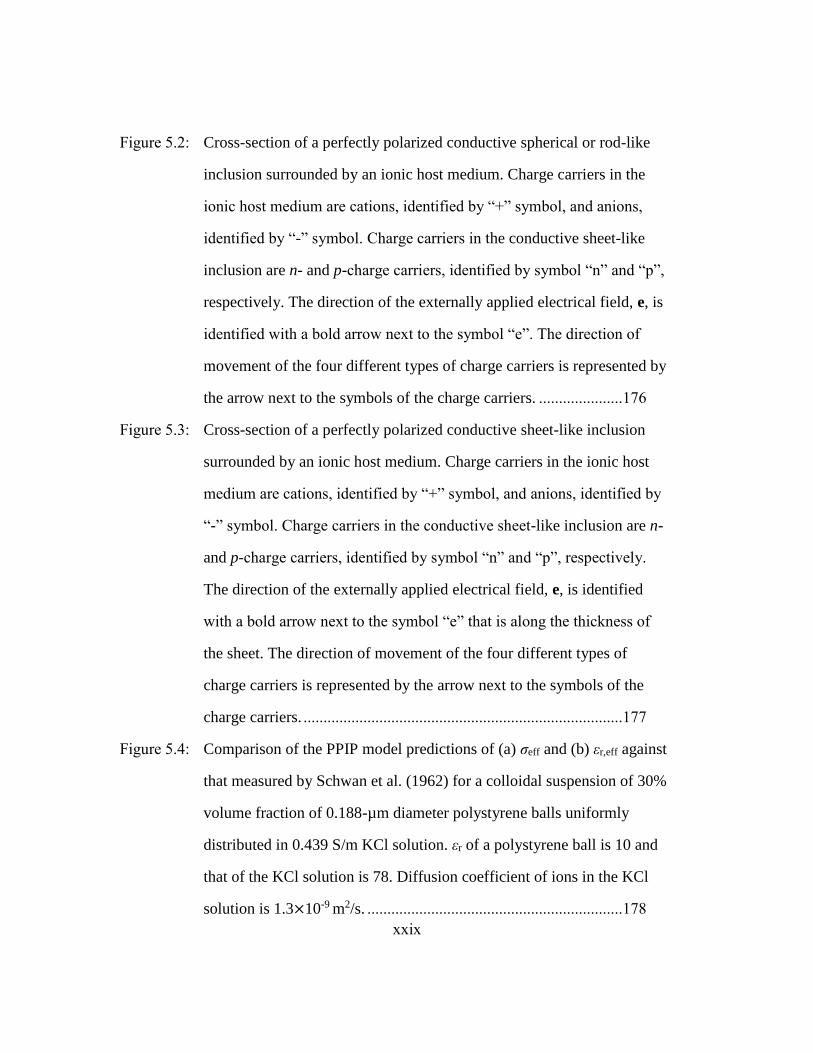
Figure 5.2: Cross-section of a perfectly polarized conductive spherical or rod-like

inclusion surrounded by an ionic host medium. Charge carriers in the

ionic host medium are cations, identified by “+” symbol, and anions,

identified by “-” symbol. Charge carriers in the conductive sheet-like

inclusion are n- and p-charge carriers, identified by symbol “n” and “p”,

respectively. The direction of the externally applied electrical field, e, is

identified with a bold arrow next to the symbol “e”. The direction of

movement of the four different types of charge carriers is represented by

the arrow next to the symbols of the charge carriers. .....................176

Figure 5.3: Cross-section of a perfectly polarized conductive sheet-like inclusion

surrounded by an ionic host medium. Charge carriers in the ionic host

medium are cations, identified by “+” symbol, and anions, identified by

“-” symbol. Charge carriers in the conductive sheet-like inclusion are n-

and p-charge carriers, identified by symbol “n” and “p”, respectively.

The direction of the externally applied electrical field, e, is identified

with a bold arrow next to the symbol “e” that is along the thickness of

the sheet. The direction of movement of the four different types of

charge carriers is represented by the arrow next to the symbols of the

charge carriers. ................................................................................177

Figure 5.4: Comparison of the PPIP model predictions of (a) σeff and (b) εr,eff against

that measured by Schwan et al. (1962) for a colloidal suspension of 30%

volume fraction of 0.188-µm diameter polystyrene balls uniformly

distributed in 0.439 S/m KCl solution. εr of a polystyrene ball is 10 and

that of the KCl solution is 78. Diffusion coefficient of ions in the KCl

solution is 1.3×10-9 m2/s. ................................................................178

xxx

Figure 5.5: Comparison of the PPIP model predictions of εr,eff against that measured

by Schwan et al. (1962) and Hanai et al. (1959) for a colloidal

suspension of polystyrene balls in KCl solution and oil-in-water

emulsion, respectively. The colloidal suspension mentioned in Schwan

et al. (1962) is made of 19.5% volume fraction of 0.56-µm diameter

polystyrene balls of εr of 10 uniformly distributed in 0.125 S/m KCl

solution. The oil-in-water emulsion mentioned in Hanai et al. (1959) is

made of 50% volume fraction of 7-µm diameter oil droplets of εr of 5

uniformly distributed in 0.002 S/m solution. Both the KCl solutions have

εr of 78, and diffusion coefficient of ions in both the KCl solutions is

1.3×10-9 m2/s. .................................................................................179


by Hanai et al. (1979) for a suspension of 59.5% volume fraction of 0.9-

µm diameter erythrocyte cells uniformly distributed in 0.4346-S/m

conductivity NaCl solution. εr of an erythrocyte cell is 3 and that of the

NaCl solution is 77. Diffusion coefficient of ions in the NaCl solution is

2×10-9 m2/s. Conductivity of the region of erythrocyte cell inside the

cell wall is 0.284 S/m. .....................................................................180


by Delgado et al. (1998) for two suspensions having 12.7% and 15.6%

volume fraction, respectively, of 115-µm diameter polymer latex balls

uniformly distributed in 0.0147-S/m conductivity KCl solution. εr of a

latex ball is 15 and that of the KCl solution is 78. Diffusion coefficient

of ions in the KCl solution is 0.8×10-9 m2/s. ..................................181

xxxi

Figure 5.8: Comparison of the PPIP-SCAIP model predictions of (a) resistivity (ρ)

and (b) phase angle (Θ) against that measured by Mahan et al. (1986) for

mixtures containing 80-µm diameter quartz grain matrix and uniformly

distributed 3.75% volume fraction of 276-µm diameter, 1000-S/m

conductivity chalcopyrite grains fully saturated with 34% volume

fraction of 0.0094-S/m conductivity NaCl solution without any active

ions. Comparison of the PPIP-SCAIP model predictions of (c) resistivity

(ρ) and (d) phase angle (Θ) against that measured by Mahan et al. (1986)

for mixtures containing 80-µm diameter quartz grain matrix and

uniformly distributed 5.8% volume fraction of 98-µm diameter, 5000-

S/m conductivity pyrite grains fully saturated with 37% volume fraction

of 0.0094-S/m conductivity NaCl solution with active ions. εr of

chalcopyrite and pyrite is 10 and 15, respectively, and that of the NaCl

solution is 80. Diffusion coefficient of charge carriers in chalcopyrite

and pyrite is 10-7 and 10-6 m2/s, respectively, and that of ions in the NaCl

solution is 2×10-11 m2/s. .................................................................182

xxxii

Figure 5.9: Comparison of the PPIP-SCAIP model predictions of (a) in-phase

conductivity (σ′) and (b) quadrature conductivity (σ″) against that

measured by Abdel Aal et al. (2014) for two mixtures containing 0.3%

volume fraction of 5000-S/m conductivity pyrite inclusions of varying

grain diameter ranging from 0.075 to 0.15 mm and 0.15 to 0.3 mm,

respectively. Pyrite inclusions were uniformly distributed in porous sand

matrix that is fully saturated with 0.0256 S/m NaCl solution. εr of pyrite

is 12 and that of the NaCl solution is 80. Diffusion coefficient of charge

carriers in pyrite is 10-6 m2/s and that of ions in the NaCl solution is 10-9

m2/s. ................................................................................................183


conductivity (σ′) and (b) quadrature conductivity (σ″) against that

measured by Abdel Aal et al. (2014) for three mixtures containing 0.5%,

1%, and 2% weight fraction, respectively, of 450-µm diameter pyrite

inclusions uniformly distributed in porous sand matrix fully saturated

with 0.0256-S/m conductivity NaCl solution. εr of pyrite is 12 and that

of the NaCl solution is 80. Diffusion coefficient of charge carriers in

pyrite is 10-6 m2/s and that of ions in the NaCl solution is 10-9 m2/s.184

xxxiii

Figure 5.11: Comparison of the SCAIP model predictions of (a) change in effective

conductivity (σeff(ω)-σeff(0)) and (b) change in effective relative

permittivity (εr,eff(ω)-εr,eff(∞)) against that measured by Tirado and

Grosse (2006) for 1% volume fraction of 1-μm diameter polystyrene

particles possessing Σs of 9×10-9 S, uniformly distributed in 0.0055-S/m

conductivity NaCl solution. εr of polystyrene ball is 10 and that of the

KCl solution is 80. Diffusion coefficient of ions in the KCl solution is

2×10-9 m2/s. ....................................................................................185

Figure 5.12: Comparison of the PPIP model predictions of critical frequency of

induced frequency dispersion against that of Wong’s (1979) modeling

results for mixtures A and B containing conductive mineral inclusions of

5000-S/m conductivity that are uniformly distributed in the electrolytic

host medium. Mixture A contains 8.3% volume fraction of conductive

inclusions distributed in the 0.002-S/m conductivity electrolytic host

having diffusion coefficient of ions of 10-9 m2/s. Mixture B contains 6%

volume fraction of conductive inclusions distributed in the 0.01-S/m

conductivity electrolytic host having diffusion coefficient of ions of

2×10-9 m2/s. For both the mixtures, εr of conductive inclusion is 15 and

that of the host is 12. Also, for both the mixtures, the diffusion

coefficient of charge carriers in the conductive inclusions is 10-6 m2/s.

.........................................................................................................186

xxxiv

Figure 5.13: PPIP model predictions of the effect of PPIP phenomenon on the

relaxation time (τ) as a function of (a) radius of the spherical conductive

inclusions, (b) diffusion coefficient (D) of charge carriers in the host and

inclusion phases, and (c) volume fraction (ϕi) of spherical conductive

inclusion phase. Default mixture is assumed to contain 1% volume

fraction of 100-S/m conductivity, 200-μm diameter conductive

inclusions uniformly distributed in 0.01-S/m conductivity electrolytic

host medium. εr of conductive inclusion phase is 10 and that of the host

is 80. Diffusion coefficient of charge carriers in conductive inclusion is

10-6 m2/s and that of ions in the host is 10-9 m2/s. ...........................187

Figure 5.14: Comparison of the PPIP model predictions of chargeability (M) against

that estimated from various laboratory measurements of the complex

resistivity response of synthetic and geological samples for varying

volume fractions (ϕi) of conductive mineral inclusions in the range of (a)

0 to 8% and (b) 0 to 30% uniformly distributed in the host medium. (c)

PPIP model predictions of chargeability of mixtures containing varying

volume fractions, in the range of 0 to 25%, of conductive inclusions

uniformly distributed in the host medium for four different values of

host conductivity. Default mixture is assumed to contain 200-µm

diameter conductive inclusions of 100-S/m conductivity uniformly

distributed in 0.01-S/m conductivity electrolytic host medium. εr of the

conductive inclusion phase is 10 and that of the host is 80. Diffusion

coefficient of charge carriers in conductive inclusion is 10-6 m2/s and

that of ions in the host is 10-9 m2/s. .................................................188

xxxv

Figure 6.1: Comparison of the PPIP and the SCAIP model predictions of the (a) LF

effective conductivity (σeff) and (b) HF effective relative permittivity

(εr,eff) of three mixtures containing 0%, 20%, and 70%, respectively,

volume fraction of non-conductive spherical grains that are uniformly

distributed in a 0.1-S/m conductivity electrolyte. Curves with “*”

superscript in their curve names identify the mixtures that were analyzed

using SCAIP model, and that without the “*” superscript identify the

mixtures that were analyzed using the PPIP model. Curves W and W*

identify mixtures with 100% volume fraction of the electrolyte, curves

S1 and S1* identify mixtures containing 20% volume fraction of the

non-conductive spherical grains and 80% volume fraction of the

electrolyte, and curves S2 and S2* identify mixtures containing 70%

volume fraction of the non-conductive spherical grains and 30% volume

fraction of the electrolyte. Default mixture is assumed to be made of 1-

mm diameter, non-conductive spherical grains possessing Σs of 10-9 S.

Relative permittivity of the non-conductive spherical grain is 4 and that

of the electrolyte is 80. Diffusion coefficient of ions in the electrolyte is

10-9 m2/s. .........................................................................................223

xxxvi

Figure 6.2: Comparison of the PPIP-SCAIP model predictions of the (a) LF σeff

against Archie’s model predictions (solid) and that of (b) HF εr,eff against

Lichtenecker-Rother model predictions (solid) for mixtures containing

varying volume fractions, ranging from 64% to 74%, of non-conductive

spherical grains that are uniformly distributed in a 0.1-S/m conductivity

electrolyte. Default mixture is assumed to contain 1-mm diameter, non-

conductive spherical grains possessing Σs of 10-9 S. Relative permittivity

of the non-conductive spherical grain is 6 and that of the electrolyte is

60. Diffusion coefficient of ions in the electrolyte is 10-9 m2/s. .....224

Figure 6.3: Comparison of the PPIP model predictions of the (a) σeff and (b) εr,eff of

mixtures containing 10% volume fraction of 200-μm diameter, spherical

inclusions that are uniformly distributed in a 0.1-S/m conductivity

electrolyte for different materials of the inclusion phase. Curves G, P, C,

X, Y, and H identify mixtures containing only graphite inclusions, pyrite

inclusions, chalcopyrite inclusions, low-conductivity material inclusions,

0.1-S/m conductivity inclusions, and non-conductive inclusions,

respectively, uniformly distributed in the electrolyte. Relative

permittivity of the electrolyte host is 80 and the diffusion coefficient of

ions in the electrolyte is 10-9 m2/s. Electrical properties assumed for the

materials of the inclusion phase for above-mentioned mixtures are

reported in Table 6.1. ......................................................................225

xxxvii

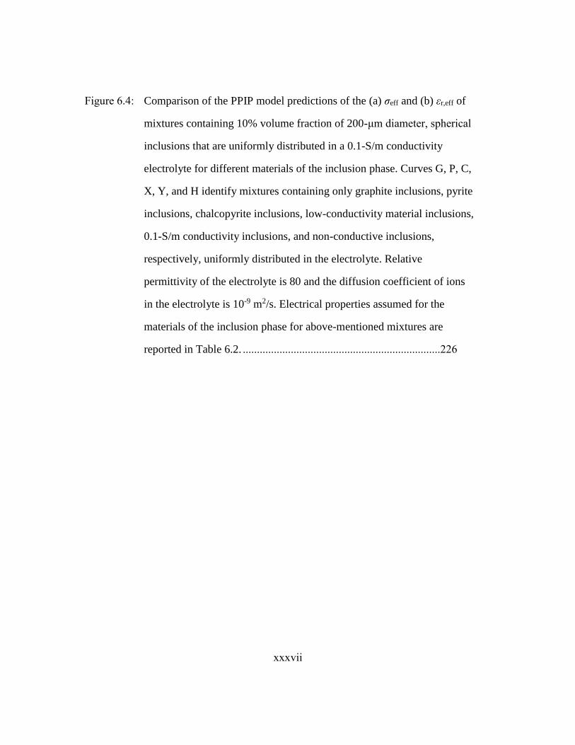
Figure 6.4: Comparison of the PPIP model predictions of the (a) σeff and (b) εr,eff of



electrolyte for different materials of the inclusion phase. Curves G, P, C,

X, Y, and H identify mixtures containing only graphite inclusions, pyrite



respectively, uniformly distributed in the electrolyte. Relative

permittivity of the electrolyte is 80 and the diffusion coefficient of ions

in the electrolyte is 10-9 m2/s. Electrical properties assumed for the

materials of the inclusion phase for above-mentioned mixtures are


xxxviii

Figure 6.5: Comparison of the PPIP-SCAIP model predictions of the (a) σeff and (b)

Θ responses of mixtures containing 70% volume fraction of 100-μm

diameter, non-conductive spherical grains and various volume fractions

of 100-μm diameter, conductive inclusions of one or more materials that

are uniformly distributed in a 0.1-S/m conductivity electrolyte. Curves

S, C, P, G, CPG, CG, and PG identify mixtures containing no

conductive inclusions, only 2% volume fraction of chalcopyrite

inclusions, only 2% volume fraction of pyrite inclusions, only 2%

volume fraction of graphite inclusions, 2% volume fractions of pyrite,

graphite, and chalcopyrite inclusions, 2% volume fractions of

chalcopyrite and graphite inclusions, and 2% volume fractions of pyrite

and graphite inclusions, respectively, uniformly distributed in the

mixture of electrolyte and non-conductive spherical grains. Relative


in the electrolyte host is 10-9 m2/s. Relative permittivity of the non-

conductive spherical grain is 5 and its Σs is 10-9 S. Electrical properties

assumed for the materials of the inclusion phase for above-mentioned

mixtures are reported in Table 6.3. .................................................227

xxxix

Figure 6.6: Comparison of the PPIP-SCAIP model predictions of the (a) σeff and (b)

Θ responses of mixtures containing varying volume fractions of either

conductive inclusions or non-conductive spherical grains, possessing

surface conductance, uniformly distributed in a matrix comprising of

70% volume fraction of non-conductive spherical grains fully saturated

with 0.01-S/m conductivity electrolyte. Curves S and Cl1 identify

mixtures containing 70% volume fraction of 1-mm diameter, non-

conductive spherical grains, possessing Σs of 10-9 S, of relative

permittivity of 5 and 70% volume fraction of 10-µm diameter, non-


permittivity of 5, respectively. Curves P, G, and Cl2 identify mixtures

containing 2% volume fraction of 100-µm diameter pyrite inclusions,

2% volume fraction of 100-µm diameter graphite inclusions, and 10%

volume fraction of 10-µm diameter non-conductive spherical grains,

possessing Σs of 10-8 S, of relative permittivity of 2, respectively,

uniformly distributed in 70% volume fraction of 1-mm diameter, non-


permittivity of 5. Relative permittivity of the electrolyte is 80 and the

diffusion coefficient of ions in the electrolyte is 10-9 m2/s. Electrical

properties assumed for the materials of the inclusion phase for above-

mentioned mixtures are reported in Table 6.4. ...............................228

xl

Figure 6.7: Comparison of the PPIP model predictions of the (a) σeff and (b) Θ

responses of mixtures containing 10% volume fraction of spherical

conductive inclusions uniformly distributed in 0.01-S/m conductivity

electrolyte for varying size and distribution of sizes of inclusions.

Conductive inclusion phase has a relative permittivity of 12,

conductivity of 500 S/m, and diffusion coefficient of charge carriers is

5×10-5 m2/s. Relative permittivity of the electrolyte is 80 and the

diffusion coefficient of ions in the electrolyte is 10-9 m2/s. Curves M1,

M2, and M3 identify mixtures containing conductive spherical

inclusions of 10-μm, 100-μm, and 1000-μm diameter, respectively.

Curves M4 and M5 identify mixtures containing conductive spherical

inclusions of uniform distribution of sizes that vary 90% about a mean

diameter of 10 μm and 100 μm, respectively. .................................229

xli


responses of mixtures containing 10% volume fraction of spherical

conductive inclusions uniformly distributed in a 0.01-S/m electrolytic

host for varying dispersity of inclusion sizes. Conductive inclusion

phase has a relative permittivity of 12, conductivity of 500 S/m, and

diffusion coefficient of charge carriers is 5×10-5 m2/s. Relative


in the electrolyte is 10-9 m2/s. Curves M6, M7, M8, and M9 identify

mixtures containing 10% volume fraction of conductive inclusions of

equal volumetric content of 10-μm and100-μm diameter inclusions; 10-

μm and1000-μm diameter inclusions; 10-μm, 100-μm, and1000-μm

diameter inclusions; and 1-μm, 10-μm,100-μm, and1000-μm diameter

inclusions, respectively. ..................................................................230

xlii


responses of four mixtures containing 10% volume fraction of 1000-μm

thick conductive sheet-like inclusions uniformly distributed in an 1-, 0.1-

, 0.01-, and 0.001-S/m conductivity electrolytic host, respectively.

Comparison of the PPIP model predictions of the (c) σeff and (d) Θ

responses of four mixtures containing 10% volume fraction of 2-, 20-,

200-, and 2000-μm thick conductive sheet-like inclusions, respectively,

uniformly distributed in a 0.1-S/m conductivity electrolytic host.

Comparison of the PPIP model predictions of the (e) σeff and (f) Θ

responses of four mixtures containing 0.1%, 1%, 2%, and 5% volume

fractions, respectively, of 1-mm thick conductive sheet-like inclusions

uniformly distributed in a 0.1-S/m conductivity electrolytic host.




diffusion coefficient of ions in the electrolyte is 10-9 m2/s. Pairs of plots

(a) and (b), (c) and (d), and (e) and (f) share the same legends,

respectively. ....................................................................................231

xliii


responses of four mixtures containing 10% volume fraction of 20-μm

diameter, conductive rod-like inclusions uniformly distributed in an 1-,

0.1-, 0.01-, and 0.001-S/m conductivity electrolytic host, respectively.

Comparison of the PPIP model predictions of the (c) σeff and (d) Θ

responses of three mixtures containing 10% volume fraction of 1-, 10-,

and 100-μm thick, conductive rod-like inclusions, respectively,

uniformly distributed in a 0.1-S/m electrolytic host. Comparison of the

PPIP model predictions of the (e) σeff and (f) Θ responses of four

mixtures containing 0.1%, 1%, 2%, and 5% volume fraction,

respectively, of 20-μm thick, conductive rod-like inclusions uniformly

distributed in a 0.1-S/m conductivity host. Conductive inclusion phase

has a relative permittivity of 12, conductivity of 5000 S/m, and diffusion

coefficient of charge carriers is 5×10-5 m2/s. Relative permittivity of the

electrolyte is 80 and the diffusion coefficient of ions in the electrolyte is

10-9 m2/s. Pairs of plots (a) and (b), (c) and (d), and (e) and (f) share the

same legends, respectively. .............................................................232

xliv

Figure 6.11: Comparison of the PPIP-SCAIP model predictions of the LF σeff and HF

εr,eff responses of mixtures S, SP1, SP2, SP3, and SCl containing no

inclusions, 5% volume fraction of 200-μm diameter spherical grains, 5%

volume fraction of 20-μm diameter long rods, 5% volume fraction of 1-

mm thick sheets, and 5% volume fraction of 10-μm diameter surface-

charge-bearing, non-conductive spherical grains exhibiting Σs of 10-8 S,

respectively, uniformly distributed in a matrix made of 70% volume

fraction of 1-mm diameter, non-conductive spherical grains that is

completely saturated with electrolyte for various electrolyte

conductivities. Pairs of Figures 11a and 11b, 11c and 11d, 11e and 11f,

and 11g and 11h identify the computed LF σeff and HF εr,eff of mixtures,

respectively, fully saturated with 0.001-, 0.01-, 0.1-, and 1-S/m

electrolyte, respectively. Conductive inclusion phase has a relative

permittivity of 12, conductivity of 5000 S/m, and diffusion coefficient of

charge carriers is 5×10-5 m2/s. Relative permittivity of the electrolyte is

80 and the diffusion coefficient of ions in the electrolyte is 10-9 m2/s.

The assumed value of relative permittivity of non-conductive spherical

grain possessing Σs of 10-9 S, identifying a sand grain, is 4 and that of

non-conductive spherical grain possessing Σs of 10-8 S, identifying a

clay-grain, is 8. All the plots share the same legend. ......................233

xlv

Figure 6.12: Comparison of the PPIP-SCAIP model predictions of the (a) LF σeff and

(b) HF εr,eff responses of mixtures S, SP1, SP2, SP3, and SCl containing

no inclusions, 5% volume fraction of 200-μm diameter conductive

spherical inclusions, 5% volume fraction of 20-μm diameter long rod-

like conductive inclusions, 5% volume fraction of 1-mm thick sheet-like

conductive inclusions, and 5% volume fraction of 10-μm diameter non-

conductive spherical inclusions possessing Σs of 10-8 S, respectively,

uniformly distributed in a matrix made of 70% volume fraction of 1-mm

diameter, non-conductive spherical grains completely saturated with

non-conductive fluid possessing a bulk relative permittivity of 3.



5×10-5 m2/s. The assumed value of relative permittivity of non-

conductive spherical grain possessing Σs of 10-9 S, identifying a sand

grain, is 4 and that of non-conductive spherical grain possessing Σs of

10-8 S, identifying a clay grain, is 8. ...............................................234

xlvi

Figure 6.13: Comparison of the PPIP-SCAIP model predictions of the (a) LF σeff and

(b) HF εr,eff responses of mixtures S, SP1, SP2, SP3, and SCl containing

no inclusions, 200-μm diameter conductive spherical inclusions, 20-μm

diameter long rod-like conductive inclusions, 1-mm thick sheet-like

conductive inclusions, and 10-μm diameter non-conductive spherical

grains exhibiting Σs of 10-8 S, respectively, uniformly distributed in a

matrix made of 70% volume fraction of 1-mm diameter non-conductive

spherical grains completely saturated with electrolyte for 1% (dotted)

and 2% (solid) volume fraction of the inclusion phase. Conductive

inclusion phase has a relative permittivity of 12, conductivity of 5000

S/m, and diffusion coefficient of charge carriers is 5×10-5 m2/s. Relative


in the electrolyte is 10-9 m2/s. The assumed value of relative permittivity

of non-conductive spherical grain possessing Σs of 10-9 S, identifying a

sand grain, is 4 and that of non-conductive spherical grain possessing Σs

of 10-8 S, identifying a clay-grain is 8.............................................235

xlvii


εr,eff responses of mixtures S, SG, SP, SC, and SX containing no

inclusions, 5% volume fraction of graphite inclusions, 5% volume

fraction of pyrite inclusions, 5% volume fraction of chalcopyrite

inclusions, and 5% volume fraction of inclusions made of a synthetic

low-conductivity material, respectively, uniformly distributed in a

matrix made of 70% volume fraction of 1-mm diameter, non-conductive

spherical grains that is completely saturated with 0.1-S/m conductivity

electrolyte. Pairs of Figures 14a and 14b, 14c and 14d, and 14e and 14f

identify the computed σeff and εr,eff, respectively, of mixtures containing

200-μm diameter spherical inclusions, 20-μm diameter long rod-like

inclusions, and 1-mm thick sheet-like inclusions, respectively. Relative

permittivity of the electrolytic host is 80 and the diffusion coefficient of

ions in the electrolyte host is 10-9 m2/s. The assumed values of relative

permittivity of the non-conductive spherical grain possessing Σs of 10-9

S, identifying a sand grain, is 4. All the plots share the same legend.

Electrical properties assumed for the four above-mentioned materials are


xlviii


εr,eff responses of mixtures S, SP1, SP2, SP3, and SP4 containing no

inclusions, 5% volume fraction of P1 pyrite inclusions, 5% volume

fraction of P2 pyrite inclusions, 5% volume fraction of P3 pyrite

inclusions, and 5% volume fraction of P4 pyrite inclusions, respectively,


diameter, non-conductive spherical grains that are completely saturated

with a 0.1-S/m conductivity electrolyte. Pairs of Figures 15a and 15b,

15c and 15d, and 15e and 15f identify the computed σeff and εr,eff,

respectively, of mixtures containing only spherical inclusions, long rod-

like inclusions, or sheet-like inclusions, respectively. The characteristic

length associated with P1, P2, P3, and P4 inclusion phase is reported in

Table 6.6. Conductive inclusion phase has a relative permittivity of 12,



diffusion coefficient of ions in the electrolyte is 10-9 m2/s. The assumed

value of relative permittivity of non-conductive spherical grain

possessing Σs of 10-9 S, identifying a sand grain, is 4. All the plots share

the same legend. ..............................................................................237

1

Chapter 1: Introduction

A detailed knowledge of reservoir rock properties is crucial for efficient

hydrocarbon production. Geoscientists and petrophysicists have developed variety of

reservoir characterization techniques, such as seismic surveys, well logging, and core

analysis, to evaluate the hydrocarbon storage potential and producibility of hydrocarbon-

bearing reservoirs. Currently, a vast majority of O&G exploration and production activities

are in geologically complex reservoirs, such as shaly sands, sand-shale laminations, and

organic-rich mudrocks. New reservoir characterization techniques are required to

accurately estimate the hydrocarbon pore volume in such reservoirs.

Existing interpretation methods for subsurface EM measurements in formations

containing dispersed and/or laminated clay minerals, clay-sized grains, and conductive

minerals rely on empirical models and lack reliable mechanistic models. Electrical

conductivity anisotropy, dielectric permittivity anisotropy, and interfacial polarization of

these formations significantly influence the EM measurements. Hence, the accuracy of

estimation of petrophysical properties based on conventional resistivity interpretation of

the EM measurements is generally improved by correlating the subsurface measurements

with laboratory measurements on core plugs. However, as-received and/or re-saturated

whole core measurements of electrical properties better represent the subsurface formation

compared to the widely used galvanic measurements on core plugs extracted from discrete

depths. For purposes of improved core-well log correlation, a non-contact and non-invasive

laboratory-based electrical apparatus needs to be developed to measure complex electrical

conductivity tensor of whole core samples at multiple frequencies. Moreover, a wideband

mechanistic model that can quantify the directional effective complex electrical

2

conductivity of geomaterials over a broad frequency range should be developed for

purposes of improving resistivity interpretation in formations containing dispersed and/or

laminated clay minerals, clay-sized grains, and conductive minerals.

1.1 PROBLEM STATEMENT

The relative proportions of hydrocarbon reserves contained in shaly sands, sand-

shale laminations, and organic-rich mudrocks are constantly increasing with the steady

decline of reserves in conventional reservoirs. Moreover, the high cost of deepwater

exploration demands high-accuracy petrophysical wellbore and laboratory measurements.

Conventional EM measurements are generally correlated with laboratory measurements on

core plugs assuming that these small-volume core plugs extracted from discrete depths of

the formation reliably represent the subsurface formation (Laswell, 2006). In certain cases,

subsurface EM measurements are re-calibrated based on galvanic measurements of core

plugs assuming negligible effects of electrode and core plug geometries, current flow path

and cross contamination issues, uncertainty in degree and area of contact between

electrodes and core plug, and poor electrical anisotropy characterization capabilities

(Kickhofel et al., 2010; Ubani et al., 2012). Further, conventional interpretation methods

neglect the effects of interfacial polarization and frequency-dispersive electrical properties

of formations (Anderson et al., 2006). From a practical view point, the validity of the

above-mentioned assumptions for geologically complex formations is being increasingly

questioned.

Several laboratory and field studies show that geomaterials exhibit electrical

conductivity anisotropy (Klein, 1996; Gianzero, 1999 ; Kennedy and Herrick, 2004), large

values of dielectric permittivity (Jackson and Hagiwara, 1998; Anderson et al., 2006; Le et

al., 2011), dielectric permittivity anisotropy (Wu et al., 1997; Lüling et al., 2005),

3

interfacial polarization (Vinegar and Waxman, 1984; Yan et al. 2014), and frequency

dispersion of the EM response (Sen, 1980; Hizem et al., 2008; Revil, 2012; Wang and

Poppitt, 2013). Conventional interpretations of electrical measurements neglect dielectric

permittivity, dielectric permittivity anisotropy, dielectric loss factor, and interfacial

polarization phenomena. In doing so, it is typically assumed that the electric field in the

formation due to an EM source in the borehole is not affected by the interfacial polarization

of clay minerals, clay-sized particles, and conductive minerals.

The effects of conductivity anisotropy on electrical measurements and the methods

to correct for such effects during resistivity interpretation of the EM measurements have

been extensively investigated in the last 20 years. Jiangqing et al. (1994) developed a

laboratory-based galvanic technique to measure the conductivity anisotropy ratio of

formations encountered in horizontal and deviated wells. They emphasized that the study

of electrical anisotropy requires high resolution measurements on larger dimension cores.

Kriegshäuser et al. (2000) developed the first logging tool capable of measuring an

electrical conductivity tensor to describe the electrical anisotropy of the subsurface

environment using three separate orthogonal coil-systems. Following that, Rosthal et al.

(2003) field tested a logging tool capable of full electrical conductivity tensor measurement

using three collocated, orthogonal coil-systems.

Electrical conductivity tensor logging tools have a vertical resolution of 2 feet.

These measurements are adversely affected by environmental effects (Wu et al., 2007).

Also, resistive cemented streaks (Yu et al., 2001), fractures (Wu et al., 2013), and bed

boundaries (Wang et al., 2003; Zhdanov et al., 2003) below the tool resolution significantly

alter the tool measurements and increase the uncertainty in subsequent interpretation. The

presence of conductive minerals, clay minerals, and clay-particles also influences the

4

conductivity tensor measurements (Anderson et al, 2007; Altman et al., 2008). Of special

significance is that in laminated reservoirs, the accuracy in the values of resistivity and

electrical anisotropy ratio of a representative shale unit is crucial for accurately interpreting

these measurements (Schoen et al., 1999). Some publications mention the substantial

uncertainty in the assessment of electrical properties of the representative shale unit. The

accuracy of resistivity interpretation of electrical logging tool measurements relies

immensely on the robustness of the inversion algorithm. All the above-mentioned factors,

warrant the development of a “standard” non-contact and non-invasive method to measure

the conductivity tensor of whole core samples at a high resolution and at multiple

frequencies to re-calibrate the log measurements, provide additional data to improve the

accuracy of inversion algorithms, measure electrical properties of the representative shale

unit for accurate laminated sand-shale analysis, and facilitate quantitative laboratory

investigation of the effects of above-mentioned factors on the conductivity tensor

measurements. Kickhofel et al. (2010) built a tool to measure the conductivity tensor of

whole core samples at a single operating frequency. They presented the reliability and

robustness of tensor EM induction measurements on whole core samples. However, the

petrophysical applications of that tool and a method for developing multifrequency

measurement capability were not studied in their work.

Interfacial polarization phenomena is the process of charge accumulation/depletion

at phase boundaries on a mesoscopic scale under the influence of an external electric field.

There are various types of interfacial polarization phenomena depending on the electrical

properties of the phase interfaces, electrical properties of the phases, and frequency of the

external electric field. Typically, for colloidal suspensions, four types of interfacial

polarization phenomena are observed within the frequency range of 10 to 1010 Hz, namely

5

α-, β-, γ-, (Shilov and Borkovskaya, 2010) and δ-polarization. The low-frequency α-

polarization is a consequence of selective conductivity of membrane structures, such as

electric double layers. This polarization mechanism is relevant to clay particles and clay-

sized grains possessing surface conductance. The mid-frequency β-polarization is

governed by thin membranes that restrict conduction of current until the frequency of

externally applied electric field increases so that the capacitive resistance of the membrane

becomes smaller than the effective ohmic resistance of the discharging medium. This

polarization mechanism is relevant to the conductive mineral inclusions and beds that give

rise to charge accumulation on their surfaces under the influence of an external electric

field. The high-frequency γ-polarization is due to Maxwell-Wagner polarization associated

with the difference in bulk conductivity of phases in contact. This polarization mechanism

is relevant to surfaces of pores and pore throats. At frequencies beyond 1 GHz, δ-

polarization (orientation polarization) occurs due to the permanent dipole moment of

materials such as water and hydrogen chloride in the mixture.

In geomaterials, different types of polarization phenomena occur. For instance,

polarization arising due to the difference in mobility of charge carriers in electrolyte, also

referred to as the concentration polarization (Khair and Squires, 2008), exchange of ions

between electric double layer around clay-sized particles and electrolyte (Revil et al.,

2012), surface conductance of clay minerals, also referred to as the membrane polarization

(Shilov et al., 2001), different types of charge carriers in host and inclusion phase (Wong

et al., 1979), oxidation-reduction reaction at the host-inclusion interfaces (Placencia-

Gomez and Slater, 2014), accumulation of charges around pore throats and at pore surfaces,

also referred to as the Maxwell-Wagner polarization (Volkmann and Kiltzsch, 2010), and

orientation polarization of water, minerals, and hydrocarbon (Hizem et al., 2008).

6

Interfacial polarization alters electromigration and electrodiffusion processes

(Schmuck and Bazant, 2012). Most interpretation methods for the electrical tools neglect

the effects of interfacial polarization; thereby, they lead to inaccurate estimation of

petrophysical properties in formations that are susceptible to significant interfacial

polarization, such as pyrite-bearing sedimentary rocks (Altman et al., 2008), clay-mineral-

bearing mudrocks (Josh and Clennell, 2015), and pyrite- and graphite-bearing organic

source rocks (Anderson et al., 2008). Subsurface galvanic and EM induction measurements

are typically interpreted at a single frequency using empirical equations ignoring the effects

of interfacial polarization due to clay minerals, conductive minerals, and clay-sized

particles (Anderson et al., 2007; Corley et al., 2010). Though, EM propagation logs are

measured and interpreted at several frequencies, the empirical equations used for

interpretation are based on mixing laws that neglect polarization due to conductive

minerals and Maxwell-Wagner polarization due to pore throats and pore surfaces (e.g.,

Hizem et al., 2008; Han et al., 2012). Empirical equations like the Archie’s equation and

Waxman-Smits equation are valid only at very low frequencies, whereas the Cole-Cole-

type dielectric dispersion models are suitable for computing frequency-dependent

electrical properties but are unsuitable for estimating petrophysically-relevant properties

of geomaterials (Toumelin, 2006).

Owing to the interfacial polarization phenomena, geomaterials exhibit large

dielectric permittivity (Le et al., 2011), non-negligible dielectric permittivity anisotropy

(Lüling et al., 2005), and large frequency dispersion of their EM response (Wang and

Poppitt, 2013). As a first step toward improved resistivity interpretation in such formations,

the resistivity model for interpreting the galvanic resistivity, EM induction, and EM

propagation measurements needs to account for the effects of interfacial polarization due

7

to surface conductivity of clay minerals and clay-sized particles and that due to

impermeable interfaces of conductive minerals with electrolyte/matrix. In doing so, these

multi-tool, multi-frequency measurements can be jointly interpreted in shaly sand, sand-

shale laminated, mudrocks, and conductive-mineral-bearing formations. Consequently, the

estimation of water saturation and TOC can be improved in these formations. The Wong

(1979) model assumes an infinitely-conducting and spherically shaped inclusion phase to

quantify the complex conductivity of a suspension of conductive minerals in an electrolyte,

whereas the Dukhin et al. (1974) model assumes a diffused double layer to quantify the

complex conductivity of a suspension of non-conductive particles in an electrolyte.

However, there is no mechanistic model that quantifies the directional complex electrical

conductivity of mixtures containing electrically conductive mineral inclusions of various

shapes uniformly distributed in a fluid-filled, porous matrix made of non-conductive grains

possessing surface conductance. No numerical modeling work has been carried out on

understanding the relative effects of interfacial polarization due to clay particles and

conductive minerals on the subsurface galvanic resistivity, EM induction, and EM

propagation logging measurements. No numerical modeling work has been carried out on

understanding the relative effects of interfacial polarization due to conductive

mineralization of varied shapes on the subsurface galvanic resistivity, EM induction, and

EM propagation logging measurements. Moreover, conventional resistivity interpretation

lacks a wideband mechanistic model that facilitates joint interpretation of multi-tool, multi-

frequency EM measurements (Wang and Poppitt, 2013). Such a wideband model is critical

to accurate estimation of TOC and water saturation in the presence of frequency-dependent

electrical properties, dielectric permittivity, and interfacial polarization phenomena.

8

To further complicate the existing challenges, there is no commercial non-contact

and non-invasive laboratory-based apparatus to measure the complex electrical

conductivity tensor of whole core samples at multiple frequencies. A continuous, non-

invasive EM measurement on a standard 2-ft-long, 4-inch-diameter whole core sample is

a better representative of the subsurface formation compared to the widely used galvanic

measurement on standard 2-inch-long, 1.5-inch-diameter core plugs. Existing special core

analyses do not characterize the electrical conductivity, anisotropy, dielectric permittivity,

and frequency dispersion characteristic of whole-core samples. There is no published work

on improving resistivity characterization of reservoir rocks by measuring electrical

properties of whole core samples in their as-received or re-saturated state. Few laboratory

investigations have been carried out to test the validity and reliability of conductivity tensor

measurements based on electromagnetic induction principles and the accuracy of its

interpretation results. Also, no laboratory investigation has been carried out to measure the

complex conductivity tensor of mixtures containing conductive mineral inclusions, such as

pyrite and graphite, in the EM induction frequency range from 10 kHz to 300 kHz, to better

understand the effects of interfacial polarization on subsurface triaxial EM induction

measurements.

Therefore, it is time to develop a new non-invasive and non-contact electrical

method to measure complex conductivity tensor of whole core samples, to

comprehensively study the relative effects of pyrite and graphite on electromagnetic

induction measurements, and to develop a wideband mechanistic model that quantifies the

effects of interfacial polarization due to clay minerals, clay-sized grains, and conductive

minerals on the EM response to facilitate joint interpretation of multi-tool, multi-frequency

subsurface EM measurements.

9

1.2 RESEARCH OBJECTIVES

The main thrust of this dissertation is to develop a laboratory measurement

technique and a quantitative interpretation method that explicitly account for the effects of

interfacial polarization due to conductive minerals, clay-sized particles, and clay minerals

uniformly distributed in a fluid-filled porous geological host. In doing so, the resistivity

interpretation of subsurface EM measurements can be improved for applications in shaly

sands, sand-shale laminations, mudrocks, and conductive-mineral-bearing formations.

Specifically, the objectives of this dissertation are as follows:

To develop a non-contact and non-invasive laboratory-based apparatus to measure

the complex electrical conductivity tensor of whole core samples at multiple

frequencies.

To develop and validate a finite-element and/or a semi-analytic EM forward model

of the developed tool.

To verify the reliability of the developed tool for purposes of estimating the

electrical properties of whole core samples. To achieve this objective, an inversion

scheme in conjunction with one of the developed EM forward models needs to be

implemented to process the multi-frequency complex conductivity measurements.

To demonstrate the petrophysical applications of the developed tool for purposes

of whole core analysis in various types of formations, such as isotropic, vuggy,

layered, etc..

To use the developed tool to estimate the directional complex conductivity of

mixtures containing conductive mineral inclusions in the EM induction frequency

range of 10 kHz to 300 kHz. This study is crucial for understanding the effects of

interfacial polarization on the subsurface EM induction measurements.

10

To develop a mechanistic model that quantifies the directional complex electrical

conductivity of mixtures containing electrically conductive mineral inclusions of

various shapes uniformly distributed in a fluid-filled, porous matrix made of non-

conductive grains possessing surface conductance.

To verify the reliability of the developed mechanistic model by quantitatively

comparing the model predictions to laboratory measurements on mixtures

containing uniformly distributed inclusions. Also, the model predictions will be

compared with the predictions of widely used empirical models.

To predict the effects of interfacial polarization due to clay particles and conductive

minerals on subsurface galvanic resistivity, EM induction, and EM propagation

logging measurements.

1.3 METHOD OVERVIEW

Results presented in this dissertation are based on the laboratory measurements,

numerical modeling, and analytical modeling of directional complex conductivity of

geomaterials. These methods allow researchers to calculate the effective electrical

properties and electrical properties of individual components of geomaterials.

In the first part of this dissertation, I develop the apparatus to measure the complex

conductivity tensor of whole core samples. The tool is designed based on the physics of

tri-axial electromagnetic induction physics (Rosthal et al., 2003). The apparatus comprises

three orthogonal (tri-axial) transmitter, bucking, and receiver coils built on the outer

surface of a tubular conduit that holds whole core samples, which are 2 feet in length and

4 inches in diameter. A resonance circuit energizes one of the three orthogonal transmitter

coils by injecting a current of known value at a specific frequency. The frequency of

excitation is selected by selecting a particular capacitor bank built in the resonance circuit.

11

A LABVIEW code is implemented to automate the selection of the frequency of the

transmitter current. When an alternating current flows through the transmitter coil, eddy

currents are induced in surrounding volume. These eddy currents induce complex-valued

voltage in the three orthogonal receiver coils. The LABVIEW-code automates the selection

of the receiver coil for measurement of the complex-valued induced voltage. The

magnitudes of the induced voltages due to whole core samples are typically on the order

of microvolts and subsequently amplified using a Lock-in amplifier. One complete cycle

of the tool measurement generates nine induced complex-valued voltage measurements,

which are subsequently converted to the complex-conductivity tensor of the whole core

sample (Kickhofel et al., 2010).

Next, I develop and validate a COMSOL-based finite element model and a

MATLAB-based semi-analytic model of the developed tool response. The semi-analytic

model is developed in MATLAB to quantify the tool response to an infinitely long, 4-inch-

diameter cylindrical volume placed in the tool conduit as a function of its horizontal

conductivity (σhor), horizontal relative permittivity (εr,hor), conductivity anisotropy ratio

(λc), permittivity anisotropy ratio (λp), and the operating frequency (Misra et al, 2015a). On

the other hand, the finite-element model is developed in COMSOL to quantify the tool

response to a 4-inch-diameter, 24-inch-long cylindrical volume, placed coaxially inside the

transmitter, receiver, and bucking coils, as a function of σhor, εr,hor, λc, λp, dip (θ), azimuth

(β), and the operating frequency (Misra et al., 2015b). Both the models describe tool

response in the induction (10-400 kHz) and propagation (0.4-2 MHz) frequency ranges.

The MATLAB-based semi-analytic model is significantly faster than the COMSOL-based

finite-element forward model.

12

The semi-analytic model is used to calibrate the nine transmitter-receiver coupling

responses (Misra et al., 2015b). It is also extensively used to estimate the horizontal and

vertical effective conductivity and relative permittivity values of samples containing

uniformly distributed conductive minerals (Misra et al., 2015a). The finite-element model

is used to estimate the geometric factor of each of the nine-transmitter receiver coupling

that is used to convert the measured values of induced receiver voltages and the transmitter

current to apparent complex conductivity measurements, which constitute the complex

conductivity tensor of a whole core sample (Misra et al., 2015b). It is also extensively used

to invert the complex conductivity tensor of layered whole core samples to obtain σhor, λc,

θ, and β (Misra et al., 2015b). Several synthetic whole core samples are prepared and

measured using the developed tool. Predictions of both the models are compared against

the laboratory measurements to validate the tool responses (Misra et al., 2015b).

After validating the tool response, petrophysical applications of the developed tool

are tested on isotropic, anisotropic, layered, vuggy, and conductive-mineral-bearing whole

core samples (Misra et al., 2015b). All this required the use of various inversion schemes

in conjunction with the developed EM forward models. First, I prepared glass-bead packs

containing conductive mineral inclusions fully saturated with brine inside 4-inch outer

diameter, 3.8-inch inner diameter, 2-ft long cylindrical glass vases. Two types of nearly

spherical pyrite inclusions are used in this work, namely Pyrite Red (average diameter =

50 µm) and Pyrite Yellow (average diameter = 130 µm) manufactured by Washington

Mills. Two types of flaky graphite inclusions are used in this work, namely #2 flake

graphite (50×200 mesh size, average surface area = 0.02 mm2) and #1 flake graphite

(50×80 mesh size, average surface area = 0.06 mm2) from Dixon Graphite. Glass beads

used in this work are 1.15-mm-diameter Megalux beads from Swarco Company. The

13

directional complex conductivity of these conductive-mineral-bearing samples are

estimated in the frequency range from 10 kHz to 300 kHz. The laboratory investigation

shows that samples containing these conductive inclusions exhibit significant frequency

dispersion of the EM response in the EM induction frequency range and large values of

dielectric permittivity (Misra et al., 2015a).

In the penultimate part of the dissertation, I develop a mechanistic model of the

directional complex conductivity of geomaterials containing conductive and clay minerals

uniformly distributed in a fluid-filled, porous matrix made of non-conductive grains

possessing surface conductance (Misra et al., 2015c). The mechanistic description of

interfacial polarization phenomena used in this new model is constructed based on

laboratory investigation performed by several researchers on mixtures containing non-

conductive particles exhibiting surface conductance (e.g., Dukhin et al., 1974; Grosse and

Foster, 1987) and on mixtures containing conductive mineral inclusions (e.g., Wong, 1979;

Chu and Bazant, 2006). Concepts implemented in the mathematical formulation of the

interfacial phenomena are attributed to Wong (1979) and to Grosse and Barchini (1992).

Our model invokes a new formulation of the Poisson-Nernst-Plank’s equation (Schmuck

and Bazant, 2012) followed by a consistent effective medium approximation (Giordano,

2003) to compute the wideband directional complex conductivity of geomaterials. The

developed model is implemented as an analytical expression in Cartesian, cylindrical, and

spherical coordinates (Misra et al., 2015c). The model is validated by comparing the model

predictions against the laboratory measurements of dispersive effective conductivity and

relative permittivity of mixtures containing uniformly distributed inclusions (e.g., Abdel

Aal et al., 2015; Revil et al., 2015a). Importantly, the developed tool responses to pyrite-

14

bearing samples are successfully quantified using the developed mechanistic model (Misra

et al., 2015a).

Finally, I perform extensive mechanistic modeling in the operating frequency

ranges of subsurface galvanic resistivity (1 Hz – 1 kHz), EM induction (10 kHz – 100 kHz),

and EM propagation (400 kHz – 10 MHz) logging tools for various petrophysical

properties of the inclusion phase and host medium. Consequently, I obtain a comparative

description of the sensitivity of measurements of these tools to petrophysical properties of

the geological mixture (Misra et al., 2015d). I find a strong dependence of these subsurface

EM measurements on the volume content, conductivity, surface conductance, shape, and

size of inclusion phase and on the conductivity of electrolyte in the host medium.

Comparison of the computed complex conductivity of mixtures against that of

uncontaminated sample indicates drastic frequency dispersion of the EM response and

large alterations of EM measurements over a broad frequency range. This necessitates the

implementation of such wideband mechanistic models to improve resistivity interpretation

in shaly sands, sand-shale laminations, and organic-rich mudrocks.

1.4 OUTLINE OF THE DISSERTATION

This dissertation consists of six additional chapters following this introductory

chapter. Chapter 2 introduces a new tool for measuring complex conductivity tensor of

whole core samples. It first discusses the theory, design, and setup of the new apparatus.

Next, I discuss and validate semi-analytic and finite-element EM forward models of the

tool response. Tool responses are then calibrated using a tilted test loop.

Subsequently, Chapter 3 documents various petrophysical applications of the

developed tool described in Chapter 2 for purposes of whole core analysis of isotropic,

anisotropic, layered, vuggy, and conductive-mineral-bearing whole core samples. Prior to

15

that, the tool measurements are validated by comparing them against the EM forward

model predictions of the tool response to synthetic samples. Numerical models of the tool

response are implemented to estimate various petrophysical properties of whole core

samples, notably host conductivity, σhor, λc, θ, and β.

Chapter 4 describes laboratory investigation of the directional complex

conductivity of mixtures containing conductive mineral inclusions in the EM induction

frequency range from 10 kHz to 300 kHz using the developed tool described in Chapter 2.

It emphasizes the estimation of effective electrical properties of conductive-mineral-

bearing mixtures as a function of the operating frequency of measurement, and shape, size,

material, and volume content of the inclusion phase. Also, it compares the electrical

properties of mixtures containing pyrite with those containing graphite.

Chapter 5 develops and validates a mechanistic model of directional complex

conductivity of mixtures containing electrically conductive mineral inclusions of various

shapes uniformly distributed in a fluid-filled, porous matrix made of non-conductive grains

possessing surface conductance. The model is implemented in Cartesian, cylindrical, and

spherical coordinates. I introduce a new effective medium formulation for mixtures

exhibiting both surface-conductance-assisted (clay particles and clay-sized grains) and

perfectly-polarized (conductive mineral inclusions) interfacial polarization phenomena.

Also, various laboratory measurements of effective electrical properties and their

frequency dispersion are reproduced using the new model.

Chapter 6 extends the new mechanistic model to describe the impact of interfacial

polarization due to clay minerals, clay-sized particles, and conductive minerals on

subsurface galvanic resistivity, EM induction, and EM propagation logging measurements.

16

Emphasis is also placed on the directional complex conductivity of mixtures containing

rod-like and sheet-like inclusions.

Finally, Chapter 7 summarizes the research achievements and contributions of the

dissertation. Conclusions are based on the laboratory investigation, mechanistic model

predictions of the directional complex conductivity, and effective electrical properties

estimated using the semi-analytic model. Also, I provide recommendations for future

research.

17

Chapter 2: Laboratory Apparatus for Multi-Frequency Inductive-

Complex Conductivity Tensor Measurements

This chapter introduces a new laboratory apparatus capable of high-resolution

multi-frequency complex conductivity tensor measurements on whole core samples and

continuous-feed cylindrical volumes in the EM induction (EMI) frequency range of 10 kHz

to 300 kHz. This experimental EM laboratory apparatus is referred to as the Whole Core

EM Induction Tool (WCEMIT). It is based on the physics of triaxial EM induction (Rosthal

et al., 2003) for a three-coil sonde (Barber, 1987) design. It is primarily a non-invasive,

non-contact measurement technique for examining whole core samples in their as-received

and re-saturated state. Tensor functionality of this tool is sensitive to the directional

electrical conductivity (σ) and dielectric relative permittivity (εr) of geomaterials, while its

multi-frequency functionality is sensitive to the dispersive electrical properties of

geomaterials.

I develop a COMSOL-based finite-element (FE) EM forward model and a

MATLAB-based semi-analytic (SA) EM forward model of the developed tool response.

The FE model is used to validate the SA model. The SA model predictions are used to

calibrate the complex impedance values measured for the nine transmitter-receiver (TR)

couplings of the WCEMIT.

2.1 INTRODUCTION

Conventional core and rotary sidewall-core samples provide petrophysicists,

engineers, and geologists with rock-based data for improved reservoir characterization.

Laboratory core measurements are used to estimate the electrical properties of reservoir

rocks, such as the parameters of the Archie’s equation or Waxman-Smits equation

(Laswell, 2006). Currently, there are no standard methods of laboratory-based electrical

18

measurements on rock core samples to estimate the electrical conductivity anisotropy, low-

frequency dielectric permittivity, and wideband frequency dispersion of electrical

properties of a subsurface formation (Ubani et al., 2012). Moreover, the widely-used

galvanic techniques for core plugs are adversely impacted by the dependence on electrode

and core plug geometries, lack of rock fabric preservation, poor electrical anisotropy

characterization capability, partial conductivity tensor measurement capability, current

path and cross contamination issues, and uncertainty in degree and area of contact between

the electrodes and core plug (Kickhofel et al., 2010). The newly developed WCEMIT

performs non-invasive, non-contact, high-resolution, multifrequency complex

conductivity tensor measurements on whole core samples. I claim that a continuous non-

invasive EM measurement on a standard 2-ft-long, 4-inch-diameter whole core sample is

a more accurate and efficient representation of a subsurface formation than the widely-used

galvanic measurement on standard 2-inch-long, 1.5-inch-diameter core plugs extracted

from discrete depths of the formation.

Induction-type conductivity sensors were first used in metal detectors in 19th

century. Within the oilfield services industry, Doll (1949) introduced the theory of

inductive resistivity measurements. The theory of conductivity tensor logging was fully

developed in the 1970s. However, the practical oilfield measurement of conductivity tensor

was introduced much later by Kriegshäuser et al. (2000) as a multicomponent induction

tool and then by Rosthal et al. (2003) as a triaxial induction tool. Currently, the conductivity

tensor tools are used worldwide to improve the interpretation of formation anisotropy, dip,

cross-bedding, bed boundaries, and fractures.

Wakamatsu (1997) developed an EM technique for dielectric spectroscopy

measurement using toroidal induction coils. This technique is free from electrode

19

polarization effects prevalent in galvanic techniques; therefore, it provides improved high-

conductivity colloidal liquid evaluation in the frequency range of 75 kHz to 30 MHz.

Wakamatsu (1997) shows that the analysis of measured dielectric relaxation response of a

colloidal liquid based on an appropriate theory of interfacial polarization provides

information on the structural and electrical properties of the colloidal particles. Asami et

al. (1999) used the non-electrode EMI method developed by Wakamatsu (1997) for real-

time monitoring of yeast cell growth. Biological cells in an external field give rise to

interfacial polarization phenomena, thereby producing a time-varying dielectric relaxation

response as a function of the yeast cell population. Won and Keiswetter (1998) investigated

applications of spectral EMI measurements to detect and characterize the geometry and

material composition of a metallic object in the frequency range of 30 Hz to 24 kHz using

collocated coils and transmitter-bucked EMI sensor. They used pulsed-width modulation

to create the desired transmitter waveform for a particular survey. They assumed a

negligible displacement current resulting from the dielectric property of the surrounding

upto a megahertz frequency. Scharfetter et al. (1999) developed an in-vivo inductive

bioimepedance spectroscopy technique applicable in the frequency range of 50 kHz to 5

MHz and conductivity range of 0.66 to 10 S/m. Further, the EMI physics is utilized

extensively for purposes of non-destructive testing in the metals industry to inspect the

quality of materials at high speed without requiring direct physical contact between the

sensor and material under inspection (Garcia-Martin et al., 2011).

With regard to laboratory analysis of rock cores, there is little published research

work on measuring electrical properties of whole cores using the EMI principles

(Kickhofel et al., 2010). Jackson et al. (2006) developed an apparatus for non-contact, non-

invasive measurement of whole-core and split-core resistivity values as a continuous log

20

at a resolution of 10 mm. They implemented a four-coil arrangement, of two pairs of

transmitter and receiver coils. The drawbacks of this apparatus were that it measures partial

conductivity tensor and has a small depth of investigation. Homan et al. (2009) introduced

the first laboratory, fully triaxial induction apparatus. It is capable of inductive-

conductivity tensor measurements on flowline, standard whole cores, and continuous-feed

cylindrical materials at a single operating frequency of 51.28 kHz. Kickhofel et al. (2010)

validated the measurements of the apparatus developed by Homan et al. (2009), and applied

it to estimate 𝜎hor and 𝜆c on a sand-shale laminated whole core at 51.28 kHz. In my work,

I extend Kickhofel et al.’s (2010) tool design by adding multi-frequency measurement

capability, applying multifrequency EM forward models of the developed tool response to

estimate electrical properties of whole core samples, and developing a robust inversion

algorithm to estimate 𝜎hor, 𝜆c, β, and θ of whole core samples. The developed apparatus is

primarily utilized to estimate the directional and dispersive σeff and εeff of conductive-

mineral-bearing samples.

2.2 THEORETICAL CONSIDERATIONS

2.2.1 Basic Theory of EM Induction Measurements

Moran and Kunz (1962) outlined the theory of the two-coil sonde from first

principles. The two-coil sonde comprises a transmitter coil and a receiver coil, each of

radius a’, positioned at a distance x apart. When an alternating current I energizes the

transmitter coil, it creates a time-varying 3D magnetic field b, which further induces eddy

currents in the surrounding volume. A small secondary magnetic field emanating from the

induced eddy currents induces a complex-valued voltage 𝑣R in the receiver coil. EMI

physics is completely described by Maxwell’s four equations, and analytical solutions

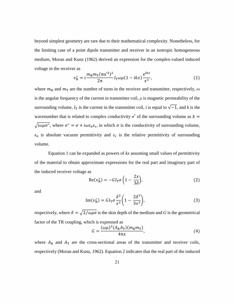
21

beyond simplest geometry are rare due to their mathematical complexity. Nonetheless, for

the limiting case of a point dipole transmitter and receiver in an isotropic homogeneous

medium, Moran and Kunz (1962) derived an expression for the complex-valued induced

voltage in the receiver as

𝑣R∗ = i

𝑚R𝑚T(π𝑎′2)2

2π𝐼T𝜔𝜇(1 − i𝑘𝑥)

ei𝑘𝑥

𝑥3, (1)

where 𝑚R and 𝑚T are the number of turns in the receiver and transmitter, respectively, ω

is the angular frequency of the current in transmitter coil, μ is magnetic permeability of the

surrounding volume, 𝐼T is the current in the transmitter coil, i is equal to √−1, and k is the

wavenumber that is related to complex conductivity σ* of the surrounding volume as 𝑘 =

√i𝜔𝜇𝜎∗, where 𝜎∗ = 𝜎 + i𝜔ε0휀r, in which 𝜎 is the conductivity of surrounding volume,

ε0 is absolute vacuum permittivity and 휀r is the relative permittivity of surrounding

volume.

Equation 1 can be expanded as powers of kx assuming small values of permittivity

of the material to obtain approximate expressions for the real part and imaginary part of

the induced receiver voltage as

Re(𝑣R∗ ) = −𝐺𝐼T𝜎 (1 −

2𝑥

3𝛿), (2)

and

Im(𝑣R∗ ) = 𝐺𝐼T𝜎

𝛿2

𝑥2(1 −

2𝛿3

3𝑥3), (3)

respectively, where 𝛿 = √2 𝜔𝜇𝜎⁄ is the skin depth of the medium and G is the geometrical

factor of the TR coupling, which is expressed as

𝐺 =(𝜔𝜇)2(𝐴R𝐴T)(𝑚R𝑚T)

4π𝑥, (4)

where 𝐴R and 𝐴T are the cross-sectional areas of the transmitter and receiver coils,

respectively (Moran and Kunz, 1962). Equation 2 indicates that the real part of the induced

22

receiver voltage is linearly related to the conductivity of surrounding volume, while the

imaginary part of the induced receiver voltage is independent of the conductivity of

surrounding volume when the surrounding volume is of negligible permittivity.

Consequently, the imaginary part of the induced receiver voltage identifies the direct

mutual coupling between transmitter and receiver coils for a two-coil sonde.

Most of the oilfield induction tools use the three-coil sonde design (Barber, 1987)

to remove the direct coupling of TR coupling from the complex-valued induced receiver

voltage measurements. A secondary receiver coil, referred to as the bucking coil, is placed

coaxially between the main receiver and transmitter coils with a magnetic moment

orientation in opposite direction to that of the main receiver coil. The number of turns and

the position of the bucking coil are such that the magnitude of the imaginary part of the

voltage induced in the main receiver coil is equal to that in the bucking coil. When the

complex-valued voltage induced in main receiver coil and that in the bucking coil are

measured in series, the direct magnetic coupling between main receiver coil and transmitter

coil is eliminated; thereby improving the sensitivity of the EMI sensor to the conductivity

of surrounding volume. After eliminating the contribution due to the direct magnetic

coupling, the σapp (or Σ) response of the surrounding volume for the TR coupling is

calculated as

𝛴 = 𝜎app = −𝑣

𝐺𝐼T≅ 𝜎 (1 −

2𝑥

3𝛿), (5)

where 𝑣 = 𝑣R∗ + 𝑣B

∗ is the induced voltage measured in the three-coil sonde after

eliminating the direct magnetic TR coupling and 𝑣B∗ is the complex-valued induced voltage

in the bucking coil. I will refer the buck-corrected receiver voltage 𝑣 simply as “receiver

voltage” from here onward. The effect of skin depth is evident in equation 5. This above

23

theory is bound by the assumptions that the surrounding environment is isotropic, non-

dispersive, and negligibly dielectric, and that the coils act as point dipoles.

2.2.2 Triaxial EM Induction Measurements

The WCEMIT (Figure 2.1) uses coaxial triaxial transmitter, receiver, and bucking

coil systems for purposes of performing complex conductivity tensor measurements on

whole core samples. Figure 2.2 shows a 24-inch-long Berea sandstone whole core sample

placed coaxially inside the 20-inch-long WCEMIT conduit. A triaxial coil system

comprises three collocated orthogonal coils, namely x-directed saddle coil, y-directed

saddle coil, and z-directed helical coil. Figure 2.3a shows a COMSOL-generated model of

a triaxial coil system containing one helical z-directed coil, one x-directed saddle coil, and

one y-directed saddle coil. Figure 2.3b shows a COMSOL-generated model of a triaxial

transmitter coil system (below) and a helical z-directed receiver coil (above), and Figure

2.3c shows a COMSOL-generated model of a whole core sample placed coaxially inside a

triaxial transmitter coil system and a helical receiver coil. The x- and y-directed saddle

coils, as shown in Figure 2.4, are created by wrapping a thin flexible circuit board around

the fiberglass conduit that holds the whole core sample during tensor measurements. The

x- and y-directed saddle coils have their magnetic moments directed along x- and y-axis,

respectively, while the z-directed helical coil has its magnetic moment directed along the

z-axis. Each saddle coil consists of mx turns, such that the height of the j-th turn of the

saddle coil is denoted as hj, the coil arc radius is a’, and 𝛽𝑗′ is the angle subtended by the

arc of the j-th turn. Figure 2.5 is a sketch of single turns of each one of the pair of x-directed

saddle coils.

The x- and y-directed saddle coils in the triaxial transmitter coil system generate

transverse magnetic moments of equal magnitude, which are also equal to the magnitude

24

of longitudinal magnetic moment of the z-directed helical coil. The induced eddy currents

in the surrounding volume due to an energized g-th transmitter coil subsequently induces

complex-valued voltages 𝑣R,𝑘∗ and 𝑣B,𝑘

∗ in the three orthogonal coils in the receiver and

bucking coil systems, respectively, where subscripts g and k can be assigned as x-, y-, or z-

directed coils. The design constraint on the saddle coils is to match the induced voltages in

the saddle receiver coils to that in the helical receiver coil for a homogeneous isotropic

surrounding volume.

Saddle bucking coils of magnetic moment opposite to that of saddle receiver coils

are used to remove the direct coupling between saddle transmitter and receiver coils.

Complex-valued induced voltages in saddle bucking coils are simultaneously measured in

series with that in the corresponding saddle receiver coils. The direct coupling between

helical transmitter and receiver coils is eliminated as described above for the three-coil

sonde design. In the WCEMIT, the complex-valued voltages induced in one of the three

collocated orthogonal coils in the receiver coil system and that induced in the

corresponding coil of the bucking coil system are simultaneously measured through the

input channel of the lock-in amplifier driven by an Agilent E3630A DC power supply.

2.2.3 Apparent Complex Conductivity Tensor

An EMI sensor based on three-coil sonde design measures the apparent complex

conductivity of surrounding volume. An inversion algorithm is required to transform the

apparent complex conductivity of the surrounding volume to the complex conductivity,

which contains the information on effective conductivity and permittivity of the

surrounding volume. Current 𝐼T,𝑔 in g-th transmitter coil induces a buck-corrected

complex-valued voltage 𝑣𝑘∗ in k-th receiver coil. Apparent complex conductivity

measurement 𝛴𝑔𝑘 is the ratio of 𝑣𝑘∗ to the mathematical product of geometrical factor of g-

25

th transmitter, k-th receiver coupling, denoted by 𝐺𝑔𝑘, and 𝐼T,𝑔. Values of 𝐺𝑔𝑘 for xx, yy,

and zz TR couplings are calculated using an EM forward model of the tool response, while

the values of 𝐺𝑔𝑘 for rest of the 6 TR couplings, namely xy, xz, yx, yz, zx, and zy, are defined

empirically (Kickhofel et al., 2010). The imaginary part of an apparent complex

conductivity 𝛴𝑔𝑘 is referred as the X-signal X𝑔𝑘, and the real part is referred as the R-signal

R𝑔𝑘. Therefore, R𝑔𝑘 identifies the resistive component, and X𝑔𝑘 identifies the reactive

component of 𝛴𝑔𝑘. The 𝛴𝑔𝑘 can also be expressed as the ratio of trans-impedance (𝑍𝑔𝑘 =

𝑣𝑘∗ 𝐼T,𝑔⁄ ) and geometrical factor of the TR coupling 𝐺𝑔𝑘 as

𝛴𝑔𝑘 = R𝑔𝑘 + iX𝑔𝑘 = − (𝑍𝑔𝑘

𝐺𝑔𝑘) = − (

𝑣𝑘∗

𝐺𝑔𝑘𝐼𝑇,𝑔). (6)

Conventional rock formations typically are of low dielectric permittivity and non-

dispersive electrical properties; therefore, they exhibit negligible phase and frequency

dependence of 𝛴𝑔𝑘 and negligible X-signal values. Hence, conventional resistivity

interpretation of the EMI sensor data generally ignores X-signal response (Anderson et al.,

2006) or uses it only for skin effect correction (Mitchell, 1997). However, in my work, I

measure samples exhibiting high dielectric permittivity and substantial frequency

dispersion due to interfacial polarization phenomena associated with disseminated

conductive minerals, clay minerals, and clay-sized particles. It is crucial for my work to

account for the negative-values of X-signal response for purposes of inverting the

measured complex electrical conductivity tensor, Σ, to obtain the effective horizontal

conductivity (𝜎hor,eff), horizontal permittivity (휀hor,eff), conductivity anisotropy (𝜆c,eff),

and permittivity anisotropy (𝜆p,eff) of the sample placed in the tool conduit. The apparent

complex conductivity tensor is a collection of apparent complex conductivity values

measured for all nine TR couplings, and is expressed as

26

𝜮 = (

𝛴𝑥𝑥 𝛴𝑥𝑦 𝛴𝑥𝑧

𝛴𝑦𝑥 𝛴𝑦𝑦 𝛴𝑦𝑧

𝛴𝑧𝑥 𝛴𝑧𝑦 𝛴𝑧𝑧

). (7)

2.3 WHOLE CORE ELECTROMAGNETIC INDUCTION TOOL (WCEMIT)

The WCEMIT performs high-resolution, multi-frequency, complex conductivity

tensor measurements on as-received or re-saturated whole core samples and continuous-

feed cylindrical volumes at seven discrete frequencies in the EM induction frequency range

of 10 kHz to 300 kHz.

2.3.1 Tool Design

The proposed apparatus comprises a 20-inch long cylindrical fiberglass sleeve

(conduit) sized to fit a 4-inch-diameter, 24-inch-long geological whole core (Figure 2.2).

The tubular shape of the WCEMIT conduit exhibits a strong proclivity toward flowline,

continuous-feed cylindrical volume, and whole core measurements. Three orthogonal tri-

axial transmitter (T or Tx), bucking (B), and receiver (R or Rx) coils are built on the outer

surface of the tubular conduit (Figure 2.2). The sample to be investigated is always placed

inside the apparatus conduit. A schematic of the apparatus is shown in Figure 2.6. The

helical z-directed transmitter coil is wound with 27 AWG HML coated magnet wire. The

center of this coil is designated as the apparatus origin (z=0). Similarly, the helical z-

directed bucking and receiver coils are wrapped at z=3 inches and z=6 inches, respectively.

On the other hand, the x- and y-directed saddle coil pairs are printed together on a thin

flexible circuit board of length slightly longer than the circumference of one turn of the

helical coil winding. Three such flexible circuit boards are wrapped at z=0, z=3, and z=6

electrically insulated about the helical coils, such that saddle coils and helical coil are

collocated with and orthogonal to each other.

27

One complete WCEMIT measurement cycle includes nine induced voltage

measurements, which are subsequently converted to apparent complex conductivity values

and then to the complex conductivity tensor of the whole core sample. The tensor

functionality of the tool, due to the triaxial coil systems, is sensitive to the directional nature

of electrical conductivity and dielectric permittivity of rock samples similar to

Schlumberger’s RtScanner downhole tool. At the same time, the WCEMIT’s multi-

frequency functionality, owing to a selectable capacitor bank built in the transmitter (Tx)

resonance circuit (Figure 2.1), is sensitive to the dielectric-dispersive characteristic of the

whole cores similar to Schlumberger’s DielectricScanner downhole tool. The transmitter

coil system is energized at one of the 7 discrete frequencies, namely 19.6, 31.2, 41.5, 58.5,

87.6, 150, or 261 kHz, during each cycle of measurement.

2.3.2 Electronic Setup

Figure 2.1 shows the laboratory setup and Figure 2.7 shows a schematic of the

laboratory setup of the WCEMIT apparatus and peripheral electronics, such as Tx

resonance circuit, receiver (Rx) amplifier, switch unit, Tx pre-amplifier, and lock-in

amplifier. The tri-axial transmitter coils are voltage driven by an Anfatec eLockIn204/2

lock-in amplifier at a single frequency. The tool operates at seven discrete drive

frequencies. For frequencies below 10 kHz, the magnitude of induced receiver voltage

drastically decreases and its phase becomes affected by environmental noise. At the other

extreme, for frequencies above 300 kHz, the operating frequency approaches the resonant

frequency of the transmitter coils; consequently, the coils exhibit capacitive properties that

decrease the stability of the measurements. The highest frequency for exciting the

transmitter coil is a factor of 2 less than the natural resonant frequency of the coil. Grounds

28

of various electronic equipment are brought to a common point at the lock-in amplifier

BNC input to avoid ground loops in the circuitry.

The signal from the lock-in amplifier is fed to a high power audio amplifier

CE1000A. Following that, the driven signal is sequentially commuted through one of the

21 resonance circuits in the Tx resonance box by an Agilent 34970A data

acquisition/switch unit to energize one of the three orthogonal coils of the transmitter coil

system at a specific frequency. Current flowing through the transmitter is measured via a

pick-off transformer, a low drift resistor, and an AD8228 (low-gain drift precision

instrumentation amplifier) within the transmitter resonance circuit by an external Agilent

34401A 6.5 digit multimeter. The energized transmitter induces complex voltages in all

the three orthogonal receiver coils. The phase and amplitude of the induced receiver

voltages are sequentially measured through the input channel of the lock-in amplifier by

means of an amplifier powered by an Agilent E3630A dc power supply. The lock-in

amplifier serves to digitally filter out all frequencies other than the specific driving

frequency generated by the Tx resonance box.

For one energized transmitter coil, three apparent complex conductivity

measurements are recorded using the electronic setup. The three orthogonal transmitter

coils are sequentially energized by Agilent 34970A switch unit. Therefore, one WCEMIT

measurement cycle generates nine apparent complex conductivity measurements that

constitutes the complex conductivity tensor of a whole core sample. This complete

experimental setup is automated in National Instruments LabVIEWTM 8.0 script so that all

of the three orthogonal receiver voltage and one transmitter current corresponding to the

energized transmitter coil can be controlled, acquired, processed into impedances, and

stored for post processing. A volume of approximately one cubic meter surrounding the

29

apparatus is cleared of conductive materials to minimize fluctuations in the background

noise. Further, tightly twisted shielded cables are implemented for all connections between

the apparatus and the electronics.

2.4 NUMERICAL MODEL OF THE WCEMIT RESPONSE

A numerical EM forward model of the WCEMIT response is crucial for estimating

petrophysical properties and electrical properties of whole core samples from the measured

complex conductivity tensor of the sample. A semi-analytical (SA) EM method was

developed to perform the WCEMIT response modeling (Misra et al., 2015c) that is

significantly faster than the WCEMIT simulation performed with COMSOL-based finite-

element (FE) EM forward model. Both SA and FE forward models quantify the helical and

saddle-type coil responses in the EM induction (1-200 kHz) and EM propagation (0.4-2

MHz) frequency ranges. For modeling purposes, a circular coil identifies a single turn of

the helical coil, and each turn of the saddle-type coils is represented by a single-turn coil

described by an azimuthal aperture angle β’, height, and radius a’ (Figure 2.5).

2.4.1 Finite-element EM Forward Model

The sequence of FE forward modeling of a physical problem is: (a) Identify the

representative physics based on a set of partial differential equations (PDE) to represent

the physics of the phenomena to be modeled, (b) define the geometry on which to solve

the physical problem, (c) assign the material properties, which identify the constants that

appear in the set of PDEs to be solved, (d) describe the boundary conditions and initial

conditions of the problem, (e) choose an element type and mesh the geometry, (f) choose

a solver and solve for the unknowns, and (g) post process the results.

30

The COMSOL AC/DC module is a powerful numerical modeling tool for finite-

element EM calculations. Kennedy et al. (2011) used COMSOL 4.2a to examine the

agreement between COMSOL 2D axial symmetric models, classical analytical solutions,

and experimental data associated with EM induction in the frequency range of 50 Hz to

500 kHz. Santandrea and Le Bihan (2010) solved the TEAM (Testing Electromagnetic

Analysis Methods) Workshop 15-1 and JSAEM (Japan Society of Applied

Electromagnetic and Mechanics) 2-5 benchmark problems using COMSOL multiphysics

3D EM FE modeling formulation. I develop a COMSOL-based FE forward model to

quantify the WCEMIT response to a 4-inch-diameter, 24-inch-long test volume as a

function of its 𝜎hor, 휀r,hor, 𝜆c, 𝜆p, θ, β, and the operating frequency. Moreover, an inversion

scheme was coupled with the FE model to estimate 𝜎hor, 𝜆c, θ, and β of samples. I used

COMOSL 3.5a to build this model. COMSOL was coupled with MATLAB to automate

simulation of synthetic cases for various parameters. I built the entire model as a MATLAB

code that interfaces with COMSOL. In comparison to the SA forward model, the FE

forward model quantifies the WCEMIT response to 4-inch diameter samples of finite

length of non-zero dip and azimuth. In this model, the sample is assumed to be coaxially

centered inside the triaxial transmitter, bucking, and receiver coil systems, and the sample

is surrounded by non-conductive air of 휀r of 1.

Since the energized transmitter coils are driven by sinusoidal current, a time

harmonic approach is used. Moreover, in order to reduce the computational complexity of

the FE model, the high number of turns of transmitter, bucking, and receiver coils are

approximated as three turns distributed uniformly over the extent of the coils. The three

turns of transmitter coils in the model produce an approximate magnetic field distribution

in space and near the three turns of receiver and bucking coil systems. In doing so, the

31

physics of the tool design is honored by capturing the EM coupling of the closest and

farthest turns of the transmitter coils with the closest and farthest turns of the bucking and

receiver coils, respectively. Induced voltage is then simply corrected by a ratio of the

number of turns in the WCEMIT to the number of turns assumed in the model.

In this model, first 𝜎hor, 휀r,hor, 𝜆c, 𝜆p, θ, β and geometry of the sample is specified.

A cylindrical cage of radius 0.75 inches larger than the radius of the sample is defined for

purposes of grid control. The FE model generally requires a fine mesh around the coils or

regions exhibiting large skin depth. Next, parameters of one transmitter and two receiver

helical and saddle coils are assigned to the model, which includes number of turns, axial

position, radius, and height of the coils. For saddle type coils, aperture angles need to be

defined for each turn, where an aperture angle is the angle subtended by a turn of saddle

type coil at the axis of the coil. Sensitivity and sonde error of direct TR coupling, namely

xx, yy, and zz, at various frequencies are calculated based on initial model predictions for

different values conductivity of the sample and operating frequencies. Sensitivity and

sonde error of the rest of the TR coupling at various frequencies are estimated empirically

(Kickhofel et al., 2010).

A simple non-reflection boundary condition was used in this model to avoid

spurious reflections from the artificial boundary to confine the computation to a particular

region around the coils. The artificial boundary surrounds the scattering region as a sphere.

In published literature, various approximate boundary conditions have been implemented

as non-reflecting boundary conditions. Most approximate non-reflecting boundary

conditions degrade rapidly as grazing incidence is approached (Grote, 1998). The

formulation used in my work requires that the ratios of the tangential components of the

electric field e to that of the magnetic field h on a sphere, which identifies the artificial

32

boundary, surrounding the antenna are forced to have a value computed from formulas for

a point magnetic dipole antenna at the center of spherical polar coordinates r, φ, and θ. The

justification is that the fields produced by a magnetic source must approach point dipole

fields at a sufficiently large distance away from the source.

It is known that the ratio 𝑍𝑠 = − 𝑒𝜑 ℎ𝜃⁄ , where e is electric field and h is the

magnetic field, on a sphere of radius R is independent of magnetic moment of dipole, and

independent of position on the sphere. The formula for the fields produced by a point

magnetic dipole source can be found in several textbooks on electromagnetics (e.g.,

Stratton, 2007). The ratio 𝑍𝑠 can be expressed as

𝑍𝑠 = i𝜔𝜇𝑅1 + i𝑘𝑅

1 + i𝑘𝑅 + (i𝑘𝑅)2, (8)

where ω is the angular frequency, µ is magnetic permeability of the medium, and k is the

wavenumber. In COMSOL, I specify a set of electrical parameters εs, μs, and σs on the

surface of the sphere. These parameters are internally used to compute the boundary

impedance 𝜔𝜇s 𝑘s⁄ , where 𝑘s = √−i𝜔𝜇s𝜎s + 𝜔2𝜇s휀s. Now, I equate the boundary

impedance to the computed Zs, and assume 𝜇𝑠 = 𝜇, without the loss of generality, to obtain 𝜔𝜇s

𝑘s= i𝜔𝜇𝑅

1 + i𝑘𝑅

1 + i𝑘𝑅 + (i𝑘𝑅)2. (9)

The condition then gives

휀s = − real(𝑓2)

𝜔2𝜇𝑅2, (10)

and

𝜎s = − imag(𝑓2)

𝜔𝜇𝑅2, (11)

where

𝑓 =1 + i𝑘𝑅 + (i𝑘𝑅)2

1 + i𝑘𝑅. (12)

33

After that, the geometry is built in the model as a combination of the outer sphere,

which identifies the artificial non-reflecting boundary, the cage cylinder, and the sample

cylinder. Following that, all axial coils and saddle coils are built in the model. The mesh

for the geometry is initialized using tetrahedral mesh elements. The quality of the meshing

is crucial for a FE model simulation. Mesh size is decided to optimize the accuracy of

numerical solutions within a reasonable computational time. I forced maximum mesh size

of 0.4 inches on coils, 1.2 inches on the curved faces of cylindrical cage, and 2 inches on

the end faces of the cylindrical cage. The meshed FE model is shown in Figure 2.8. Then,

the code performs an edge analysis of the axial coil edges and horizontal and vertical edges

of the saddle coil to define properties of the edges, namely edge identifier, edge type, and

presence of current in the edge. Non-reflecting boundary condition is applied to the

artificial boundary as a impedance boundary of εs and σs values as derived in equations 10

and 11. The remaining boundaries are defined as a continuous boundary. Finally, the

permittivity and conductivity of the sample are described as tensors, and the surrounding

air is assumed isotropic of ε0 of 1 and σ of 10-5 S/m. Figures 2.9 and 2.10 show the modeling

results of the b-field and e-field for an energized z-directed and y-directed transmitter coils,

respectively.

2.4.2 Semi-analytic EM Forward Model

A semi-analytic (SA) forward model was applied to quantify the full-triaxial

WCEMIT response to an infinitely-long, 4-inch-diameter cylindrical volume, placed in the

WCEMIT conduit, as a function of its 𝜎hor, 휀r,hor, 𝜆c, and 𝜆p. The SA model assumes the

surrounding volume as two infinitely-long, anisotropic, axially-symmetrical, concentric

cylindrical regions in electrical communication with each other. In addition, this model is

used to quantify the WCEMIT response to a tilted test loop (TTL); this modeled response

34

is then used to calibrate the WCEMIT response. The SA model is applicable at induction

frequencies as well as propagation frequencies.

In one formulation, for an infinite homogeneous medium with TI anisotropy

containing a source, electric field e at any point r1 due to a source current density j at r2 can

be computed analytically as

𝒆(𝒓1) = −i𝑘0 ∫ Γ̿ (𝒓1, 𝒓2). 𝒋(𝒓2)𝑑3𝑟2, (13)

where 𝑘0 = 𝜔√ε0μ0 and Γ̿ is the Green’s dyadic that can be constructed with two vector

fields 𝒎ℎ and 𝒏𝑒, which are derived from two scalar Hansen potentials 𝜑h and 𝜑e,

respectively, expressed as

𝒎ℎ = ∇ × 𝒖𝑧𝜑h, (14)

𝒏𝑒 =1

𝑘0∇ × �̿�−1. (∇ × 𝒖𝑧𝜑e), (15)

where �̿� is magnetic permeability tensor of the medium and 𝒖𝑧 is the z-directed unit vector

in cylindrical coordinates. 𝜑h and 𝜑e can be expressed as the solutions of the scalar

Helmholtz equation in cylindrical coordinates. In the second formulation, for each source-

free homogeneous anisotropic cylindrical subregions, the electric field e and magnetic field

h are expressed as linear combinations of vector fields 𝒎ℎ and 𝒏𝑒. Such an expression has

several unknown coefficients.

The two above-mentioned formulations are compared on the cylindrical surface

containing the transmitter coils to obtain the discontinuity in the values of unknown

coefficients of the linear combination, which was obtained in the second formulation, due

to current density in the transmitter coils. Next, Maxwell’s equations are solved to obtain

the values for the unknown coefficients of the linear combination, which was obtained in

the second formulation. The following boundary conditions are used to solve the system

of Maxwell’s equation: (a) continuity of tangential components of e and h at the outer

35

surface of the inner cylinder that identifies the whole core sample, (b) no incoming wave

at the outermost surface of the outer cylinder, and (c) finite solution along the entire z-axis.

After obtaining the values of unknown coefficients, the voltage induced in a receiver coil

is obtained as a volume integral along the geometry of the receiver coil expressed as

𝑣R = 𝑍0 ∮ 𝒆. 𝑑𝒓 = 𝑍0 ∫ 𝜒R . 𝒆𝑑3𝑟, (16)

where 𝑍0 = √μ0/ε0 = 376.7 ohms is the impedance of free space. A MATLAB-based

adaptive Lobatto Quadrature method (Gander and Gautschi, 1998) was implemented to

solve the integral forms.

2.4.3 Model Validation

The accuracy of the FE model is confirmed by comparing model predictions and

analytical solution for a circular loop of current in an infinite isotropic medium at several

frequencies in the range of 10 to 300 kHz. Analytical solution to this physical problem is

derived by Moran and Kunz (1962). For further validation of the FE model, I compute the

real part of the induced voltage response of the three direct couplings, namely xx, yy, and

zz, for various values of conductivity of a 24-inch-long, 4-inch-diameter cylindrical volume

(sample) placed inside the coils. The log-log plot in Figure 2.11 depicts a linear relationship

of the real part of the induced voltage response of zz-coupling to the conductivity of the

sample for conductivity values of 0.1, 1, and 10 S/m, respectively. This observed linear

relationship is analogous to the linearity of induced voltage and conductivity of

surrounding medium for a two-coil sonde configuration assuming point dipole

approximation, as derived by Moran and Kunz (1962). The induced voltage responses of

xx- coupling and yy-coupling also display linear relationships with conductivity of the

sample. Such linear relationships have been used as a benchmark for the validity of the

predictions of numerical models of EMI coils. The slopes of the straight lines plotted in

36

Figure 2.11 are equal to the geometrical factor (Table 2.1) for the zz-coupling at the seven

discrete frequencies, namely 19.6, 31.2, 41.5, 58.5, 87.6, 150.4, and 261 kHz. The

computed values of geometrical factors for zz-coupling and yy-coupling of 1.5×10-4 and

3.6×10-5 m.Ω/s, respectively, at 58.5 kHz is close to the values of geometrical factors for

zz-coupling and yy-coupling of 1.42×10-4 and 3.54×10-5 m.Ω/s, respectively, at 51.28 kHz

obtained by Kickhofel et al. (2010).

For further validation of the FE model, I investigated the relationship of the

geometrical factor of the zz-coupling with the operating frequency. Moran and Kunz (1962)

showed analytically that the geometrical factor of the zz-coupling of a two-coil sonde in an

isotropic homogeneous medium is directly proportional to the square of the operating

frequency. Although the FE model is for a cylindrical sample placed inside a three-coil

sonde, the log-log plot in Figure 2.12 illustrates that the geometrical factor of zz-coupling

computed based on the FE model predictions of the WCEMIT response to 1-S/m

conductivity cylindrical volume is directly proportional to the square of the operating

frequency. Another important validation involves comparing FE model predictions against

the Maxwell-Garnett effective medium (Giordano, 2003) predictions of the effective

conductivity of a 1-S/m-conductivity 4-inch diameter cylindrical sample containing

homogeneously distributed spheres for different values of conductivity and radius of the

spherical inclusion phase. Figure 2.13 illustrates the COMSOL-generated meshed model

of the 4-inch-diameter cylinder containing 0.35-inch-radius spheres. Figure 2.14 indicates

a good agreement between the effective medium predictions and FE model predictions for

conductivity values of spherical inclusions in the range of 0.1 S/m to 100 S/m and for radius

of spherical inclusions in the range of 0.35 to 0.6 inches. The observed agreement however

deteriorates for spherical inclusion phases of higher conductivity and larger radius due to

37

inherent discrepancies of the Maxwell-Garnett effective medium predictions arising from

the EM interactions of the inclusions and due to the high contrast in electrical properties of

the inclusion and host phase.

After validating the FE model predictions, I compare the SA model predictions

against that of the FE model for purposes of validating the SA model predictions. First, the

log-log plot in Figure 2.15 shows the good agreement between both the model predictions

of the real part of the induced voltage response of zz-coupling to three cylindrical volumes

of conductivity of 0.1, 1, and 10 S/m, respectively, for different values of the operating

frequency. Further, the SA model predictions of R- and X-signal responses yy-coupling

and zz-coupling to two cylindrical volumes of 𝜎hor of 1 S/m, 휀r of 105, and dielectric loss

factor (δ) of 0 (Figure 2.16) and 0.1 (Figure 2.17), respectively are compared with that of

the FE model. The SA model predictions for both of the cases match very well with the FE

model predictions for both the yy-coupling and zz-coupling responses, as illustrated in

Figures 2.16 and 2.17.

Figure 2.16 depict the FE and SA model predictions of R- and X-signal response to

a sample of 𝜎hor of 1 S/m, 휀r of 105, and δ of 0. Both the models in Figure 2.16 predict

large negative values of the X-signal response, varying from -0.01 S/m to -1.5 S/m with

the variation in the operating frequency from 19.6 kHz to 261 kHz. Moreover, Figure 2.16

indicates that an order of magnitude increase in the operating frequency produces a two-

order of magnitude increase in X-signal response. Such a substantial frequency dispersion

in X-signal is a consequence of the large value of the relative permittivity of the sample.

Nonetheless, in Figure 2.16, the frequency dispersion in R-signal response is negligible

because the δ of the medium is assumed to be zero. In contrast, the FE and SA model

predictions of R- and X-signal response to a sample of 𝜎hor of 1 S/m, 휀r of 105, and δ of

38

0.1, as presented in Figure 2.17, indicate a large frequency dispersion in R-signal response

as a consequence of the non-zero δ of the sample. In addition, the magnitude of R-signal

response increases with an increase in the operating frequency. On comparing X- and R-

signal responses depicted in Figures 2.16 with that in Figure 2.17, I infer that variation in

δ has negligible influence on the X-signal response, whereas variation in 휀r has negligible

influence on the R-signal. Due to the absence of electrical and dielectric anisotropy in the

samples, the computed yy-coupling response matches very well with the computed zz-

coupling responses.

2.5 WCEMIT CALIBRATION

During the construction of coils, the bucking coil system is translated along the tool

axis until the complex-valued voltage response on the z-directed receiver coil for an

energized z-directed transmitter is at a minimum, which ensures that the direct magnetic

field coupling between the two coils is minimized for purposes of an improved signal-to-

noise ratio. The z-directed buck coil is then fixed at that position. Following that, the saddle

coils of the bucking coil system are slightly rotated about the tool axis to balance the

complex-valued voltage response of the x-directed and y-directed receiver coils for the

energized z-directed transmitter coil. The nine TR coupling responses are then calibrated

using the tilted test loop (TTL) method to find the gain amplitude and phase corrections

(Kilic, 2014).

The WCEMIT response to a TTL provides reference measurements for calibrating

the nine TR coupling responses. The TTL comprises a copper wire in series with a resistor

of known impedance oriented at a 45°-dip on an 8-inch-diameter tube coaxial to the tool

axis. Figure 2.18 shows the laboratory set-up of the WCEMIT placed coaxially inside the

8-inch-diameter tube that holds the TTL at 45°-dip. The impedance of the resistor changes

39

with operating frequency; therefore I measure the frequency-dependent impedance of the

resistor at various frequencies (Table 2.2) using a calibrated HP4194A impedance/gain-

phase analyzer. These measured impedance values for the resistor is used in the SA model

to quantify the WCEMIT response to the TTL for various positons of the TTL at azimuthal

orientations of the TTL of 0°, 45°, and 90°. Using the SA model predictions, I design the

calibration process such that all the nine responses of the WCEMIT can be excited with

the TTL at azimuths of 0°, 45°, and 90° by placing the TTL at specific distances away from

the center of transmitter coil along the tool axis. The various azimuthal orientations and

positions of the TTL for purposes of calibrating the nine TR coupling responses are shown

in Table 2.3.

To obtain the gain correction for a specific TR coupling, the TTL is positioned and

oriented as displayed in Table 2.3 for the corresponding TR coupling. Next, the impedance

of TTL with respect to the corresponding TR coupling is measured using the WCEMIT.

Figure 2.19 shows a schematic of the TTL translation and azimuthal orientation about the

WCEMIT. The complex-valued gain required for calibrating a specific TR coupling is

expressed as

𝑔𝑔𝑘 =𝑍𝑔𝑘

𝑚𝑜𝑑

𝑍𝑔𝑘𝑚𝑒𝑎𝑠 − 𝑍𝑔𝑘

𝑎𝑖𝑟, (17)

where g denotes the energized g-directed transmitter, k denotes the k-directed receiver at

which the induced voltage is measured, 𝑍𝑔𝑘𝑚𝑜𝑑 is the theoretical impedance response

calculated using the SA model of the gk-coupling response, 𝑍𝑔𝑘𝑚𝑒𝑎𝑠 is the measured value

of raw impedance of the TTL at a particular location and orientation with respect to the gk-

coupling, and 𝑍𝑔𝑘𝑎𝑖𝑟 is the measured value of raw impedance of the background with respect

to the gk-coupling. This complex-valued gain is unique to the apparatus for a given TR

coupling and operating frequency. Tables 2.4 and 2.5 contain the amplitude and phase of

40

gain correction derived for the nine TR couplings at seven discrete operating frequencies,

namely 19.6, 31.2, 41.5, 58.5, 87.6, 150.4, and 261 kHz. Importantly, the amplitude of gain

correction values obtained at operating frequencies of 31.2, 41.5, 58.5, and 87.6 kHz are

close to 1, which indicates the reliability of this calibration process, wherein the measured

impedance values are compared against the SA model predictions.

To calibrate both the amplitude and the phase of subsequent WCEMIT apparent

complex conductivity measurements, the complex-valued gain correction is applied as

𝛴𝑔𝑘 = 𝑔𝑔𝑘 (𝑍𝑔𝑘

𝑚𝑒𝑎𝑠 − 𝑍𝑔𝑘𝑎𝑖𝑟

𝐺𝑔𝑘), (18)

where 𝛴𝑔𝑘is the apparent complex conductivity of the sample with respect to the gk-

coupling, 𝐺𝑔𝑘 is the geometrical factor of the gk-coupling, 𝑔𝑔𝑘 is the complex-valued gain

correction for the gk-coupling, and 𝑍𝑔𝑘𝑎𝑖𝑟 is the measured value of raw impedance of the

background with respect to the gk-coupling.

2.6 CONCLUSIONS

I described the theory, tool design, and electronic setup of the WCEMIT capable of

non-invasive, non-contact, high-resolution, multifrequency, complex conductivity tensor

measurements on whole core samples. I developed and validated a COMSOL-based finite-

element EM forward model and a MATLAB-based semi-analytic EM forward model of

the WCEMIT response. Predictions of the finite-element forward model match those of the

semi-analytic forward model. Finally, the nine TR coupling responses were calibrated

using a tilted-test-loop method at seven discrete frequencies, namely 19.6, 31.2, 41.5, 58.5,

87.6, 150.4, and 261 kHz.

Improved resistivity interpretation in shaly, sand-shale laminated, source rock, and

mudrock formations requires high-resolution non-invasive whole core measurement

41

techniques. The developments in this chapter encourage laboratory investigation of

petrophysical applications of this new electromagnetic measurement method.

42

Table 2.1: The values geometrical factor K of yy-coupling and zz-coupling at various

frequencies.

Table 2.2: TTL impedance at various frequencies.

Frequency (kHz) TTL impedance (Ω)

11.094 10.0173 - 0.0655i

19.58 10.0098 - 0.0656i

31.267 10.0082 - 0.1746i

41.54 10.0116 - 0.0870i

58.5 10.0082 - 0.1746i

88.119 10.0085 - 0.3495i

150.424 10.01167 - 0.5175i

261.347 10.0141 - 1.5280i

Frequency (kHz)

K

(m.Ω/S)

19.6 31.2 41.5 58.5 87.6 150.4 261

yy 4.0×10-6 1.0×10-5 1.8×10-5 3.6×10-5 8.0×10-5 2.4×10-4 7.1×10-4

zz 1.6×10-5 4.1×10-5 7.4×10-5 1.5×10-4 3.3×10-4 9.7×10-4 2.9×10-4

43

Table 2.3: Azimuthal orientation and location of the TTL for purposes of calibrating

specific TR coupling responses.

TR Coupling Azimuth (°) TTL-location (in.)

xx 0 3.10

xy 45 3.20

xz 0 2.42

yx 45 3.20

yy 90 3.10

yz 90 2.42

zx 0 3.82

zy 90 3.82

zz 0 3.11

44


operating frequencies of 19.6, 31.2, 41.5, and 58.5 kHz.

Frequency (Hz)

19.6 31.2 41.5 58.5

TR

Coupling

Gain

amp.

Gain

phase

Gain

amp.

Gain

phase

Gain

amp.

Gain

phase

Gain

amp.

Gain

phase

xx 1.0 154.8 1.0 142.0 1.1 118.3 1.2 93.5

xy 3.2 179.2 1.0 142.2 1.2 93.5 1.2 93.5

xz 3.0 180.0 0.9 140.0 1.1 92.2 1.1 92.2

yx 3.3 180.0 0.2 104.0 1.2 93.9 1.2 93.9

yy 1.0 153.6 1.0 141.4 1.1 117.6 1.2 93.3

yz 3.0 179.1 0.9 139.7 1.1 92.6 1.1 92.6

zx 2.9 -20.3 0.9 -83.1 1.1 -119.5 1.1 -119.5

zy 2.9 -19.1 0.9 -82.6 1.1 -120.4 1.1 -120.4

zz 0.9 -25.9 0.9 -69.0 0.9 -86.7 1.0 -111.6

45


operating frequencies of 87.6, 150.4, and 261 kHz.

Frequency (Hz)

87.6 150.4 261.0

TR

Coupling

Gain

amp.

Gain

phase

Gain

amp.

Gain

phase

Gain

amp.

Gain

phase

xx 1.4 100.9 2.2 4.7 3.8 -51.8

xy 1.4 101.1 0.4 -57.8 3.5 -52.1

xz 1.3 98.8 0.6 -62.2 5.3 -56.5

yx 1.4 100.6 0.4 -74.0 3.7 -68.2

yy 1.4 95.5 2.2 -2.7 3.6 -66.9

yz 1.3 101.9 0.5 -77.1 4.7 -71.4

zx 1.2 -99.5 0.3 148.0 3.1 153.7

zy 1.2 -98.4 0.4 -177.1 3.5 -171.4

zz 1.1 -95.4 1.8 174.1 2.8 147.6

46

Figure 2.1: Photograph of the WCEMIT comprising a 20-inch-long WCEMIT conduit,

coil systems, and peripheral electronics.

Figure 2.2: Photograph of a Berea sandstone whole core placed in the 4-inch-inner-

diameter, 20-inch-long WCEMIT conduit. Letters R, B, and T identify

orthogonal receiver, bucking, and transmitter coil systems, respectively.

T R B

47

Figure 2.3: COMSOL-generated model of (a) a simplified triaxial coil system

containing one helical z-directed coil, one x-directed saddle coil, and one y-

directed saddle coil, (b) a simplified triaxial transmitter coil system (below)

and a helical z-directed receiver coil (above), and (c) a whole core sample

placed coaxially inside simplified triaxial transmitter (below) and receiver

(above) coil systems.

b

a c

48

Figure 2.4: (a) Photograph of the WCEMIT shows one of the pair of x-directed

transmitter saddle coils (below) and that of the x-directed receiver saddle

coils (above), as indicated by blue arrows. (b) A zoomed-in schematic of a

saddle coil.

Figure 2.5: A sketch of single turns of each one of the pair of x-directed saddle coils,

where the height of the single turns is h, the coil arc radius is a, β is the

angle subtended by the arc of the single turns, and bx1 and bx2 are the

magnetic moments of each one of the pair of x-directed saddle coils.

a

b

49

Figure 2.6: A schematic of the WCEMIT, where the fiberglass sleeve between the coils

and the whole core sample is made transparent to show a 4-inch-diameter

whole core sample.

Figure 2.7: A schematic of the laboratory setup for measuring complex conductivity

tensor using the WCEMIT.

50

Figure 2.8: A COMSOL-generated meshed model of the WCEMIT. The figure depicts

the outer artificial non-reflecting boundary, the triaxial transmitter, receiver,

and bucking coil systems, and the 4-inch-diameter, 20-inch-long cylindrical

volume identifying the whole core sample.

51

Figure 2.9: (a) FE model results for an energized z-directed transmitter coil, where the

streamline track the b-field in the zx-plane and the slice of yx-plane, in

green, shows the magnitude of the imaginary part of x-component of the e-

field, shown by arrows, as color map. (b) A zoom-in around the coils of the

FE model results.

Figure 2.10: (a) FE model results for an energized y-directed transmitter coil, where the

streamline track the b-field in the zy-plane and the slice of zx-plane, in

green, shows the magnitude of the imaginary part of z-component of the e-

field, shown by arrows, as color map. (b) A zoom-in around the coils of the

FE model results.

a b

a b

52

Figure 2.11: FE model predictions of the real part of the buck-corrected induced voltage

response of zz-coupling to three isotropic cylindrical volumes of 𝜎hor of 0.1,

1, and 10 S/m, respectively, computed at 19.6, 31.2, 41.5, 58.5, 87.6, 150.4,

and 261 kHz.

Figure 2.12: FE model predictions of the geometrical factor of the zz-coupling as a

function of operating frequency.

10-1

100

101

10-7

10-6

10-5

10-4

10-3

10-2

Conductivity (S/m)

Re

al in

du

ced

vo

ltag

e (

V)

19.6 kHz

31.2 kHz

41.5 kHz

58.5 kHz

87.6 kHz

150.4 kHz

261 kHz

101

102

10-6

10-5

10-4

10-3

Frequency (kHz)

Geo

metr

ical fa

cto

r (m

. /S

)

Computed geometrical factor

log(K)=2log(f)+c

53

Figure 2.13: A COMSOL-generated meshed model of the 4-inch-diameter isotropic

cylinder containing randomly distributed 0.35-inch-radius isotropic spheres

placed inside the triaxial transmitter, receiver, and bucking coil systems.

Figure 2.14: Comparison of the FE model predictions against the Maxwell-Garnett

effective medium predictions of effective conductivity of a 1-S/m-

conductivity cylindrical volume containing randomly distributed spheres at

58.5 kHz for spheres of 0.001, 0.1-, 1-, 10-, or 100-S/m-conductivity. Both

the cylindrical volume and the spheres have relative permittivity of 1. The

FE model predictions are for the yy-coupling response.

10-3

10-2

10-1

100

101

102

0.8

1.1

1.4

1.7

2

i (S/m)

e

ff (

S/m

)

yy ri=0.354 in.

EMT ri=0.354 in.

yy ri=0.394 in.

EMT ri=0.394 in.

yy ri=0.512 in.

EMT ri=0.512 in.

54

Figure 2.15: Comparison of the SA model predictions against the FE model predictions

of the real part of the induced voltage response of zz-coupling to three

isotropic cylindrical volumes of 𝜎hor of 0.1, 1, and 10 S/m, respectively,

computed at 19.6, 31.2, 41.5, 58.5, 87.6, 150.4, and 261 kHz.


of (a) R-signal and (b) X-signal responses of yy-coupling and zz-coupling to

isotropic cylindrical volume of 𝜎hor of 1 S/m, 휀r of 105, and δ of 0 computed

at 19.6, 31.2, 41.5, 58.5, 87.6, 150.4, and 261 kHz.

101

102

10-7

10-6

10-5

10-4

10-3

10-2

Frequency (kHz)

Re

al in

du

ced

vo

ltag

e (

V)

0.1 S/m (FE)

1 S/m (FE)

10 S/m (FE)

0.1 S/m (SA)

1 S/m (SA)

10 S/m (SA)

101

102

0.95

0.975

1

1.025

1.05

Frequency (kHz)

R-s

ign

al (S

/m)

(a)

FE-YY

FE-ZZ

SA-YY

SA-ZZ

101

102

-1.5

-1

-0.5

0

Frequency (kHz)

X-s

ign

al (S

/m)

(b)

55


of (a) R-signal and (b) X-signal responses of yy-coupling and zz-coupling to

isotropic cylindrical volume of 𝜎hor of 1 S/m, 휀r of 105, and δ of 0.1

computed at 19.6, 31.2, 41.5, 58.5, 87.6, 150.4, and 261 kHz.

Figure 2.18: Laboratory set-up of the WCEMIT placed coaxially inside an 8-inch-

diameter tube that holds the tilted test loop (TTL) at a 45°-dip.

101

102

1

1.04

1.08

1.12

1.16

Frequency (kHz)

R-s

ign

al (S

/m)

(a)

FE-YY

FE-ZZ

SA-YY

SA-ZZ

101

102

-1.5

-1

-0.5

0

Frequency (kHz)

X-s

ign

al (S

/m)

(b)

56

Figure 2.19: The TTL (yellow) is placed coaxially around the WCEMIT such that the dip

of the TTL, which is the angle between the direction of magnetic moment of

the TTL (blue arrow) and the z-axis, is 45°, and the azimuthal orientation

(red arrow) of the TTL, which is the angle between the direction of

magnetic moment of the TTL (blue arrow) and the x-axis, is either 0°, 45°,

or 90°. The TTL translates along the tool axis (z-axis, green arrow).

57

Chapter 3: Petrophysical Applications of Multi-Frequency Inductive-

Complex Electrical Conductivity Tensor Measurements on Whole Core

Samples

Until now, electrical measurement methods on whole core samples so far have not

been used for purposes of laboratory-based petrophysical characterization. In this chapter,

I use the laboratory apparatus WCEMIT, described in Chapter 2, to measure the multi-

frequency inductive-complex electrical conductivity tensor of whole core samples of

various rock facies. First, the WCEMIT measurements are validated by comparing the

WCEMIT responses to various synthetic samples against the numerical predictions of the

semi-analytic (SA) EM forward model, introduced in Chapter 2. I then invoke an inversion

scheme that processes WCEMIT measurements to estimate the electrical properties of

natural and synthetic whole core samples in the EM induction frequency range of 10 kHz

to 300 kHz. Finally, the Archie’s equation, laminated sand-shale model, tensor resistivity

model, and Maxwell-Garnett effective medium model are implemented for estimating

petrophysical properties of the whole core samples of various rock facies. I also apply the

SA forward model to investigate petrophysical applications of the WCEMIT measurements

on whole core samples exhibiting large dielectric permittivity, permittivity anisotropy,

dielectric loss factor, and frequency dispersive dielectric properties. Further, I invoke the

finite-element (FE) EM forward model, introduced in Chapter 2, to investigate a whole

core logging method that will improve the resistivity characterization of turbiditic and

multi-layered formations.

3.1 INTRODUCTION

The primary objective of this chapter is to present the petrophysical applications of

the WCEMIT through laboratory and numerical modeling investigations. I claim that

58

electrical measurements of as-received or cleaned whole core samples using the non-

contact and non-invasive electromagnetic induction technique of the WCEMIT will

substantially improve the subsurface resistivity interpretation. Existing laboratory

measurements of electrical properties rely on galvanic measurements on core plugs. In

complex lithologies, core plugs do not preserve the bulk electrical properties of the

formation, such as anisotropy, Archie’s porosity and water saturation exponent, and

dielectric dispersion parameters. As described in Chapter 2, galvanic methods also suffer

from other issues that adversely affect the accuracy of estimation of electrical properties.

The API recommended practice for core analysis procedure (RP40, 1960) states

that whole cores are essential in vuggy carbonates, fractured reservoirs, and conglomerates,

where significant large scale heterogeneity exists. Keelan (1982) listed a comparative data

to highlight the need for whole core measurements in quantifying fracture effects. He

summarized that the sample size should be such that the total pore space is small compared

to the bulk volume, and that any estimations of directional properties, such as resistivity

and permeability, are better represented by measuring whole cores instead of core plugs.

Bergosh et al. (1985) mentioned that core plug measurements rarely capture fracture effects

and are unrepresentative of fractured formations due to the limited sample size of core

plugs. Additionally, the permeability anisotropy and variation in fluid distribution reduce

the accuracy of core plug measurements. Honarpour et al. (2003) emphasized that whole

core analysis is critical to characterizing porosity and directional permeability in

heterogeneous, fractured, and anisotropic rocks because small-scale heterogeneity is not

appropriately represented in plug measurements. They demonstrated that the whole core

permeability measurements are better representative of heterogeneous carbonate

formations compared to core plug measurements because they correctly average the high

59

and low permeability zones into overall volume. The greatest advantage of electrical

measurements on whole cores is obtaining a representative porosity exponent in

heterogeneous rocks (Honarpour et al., 2003).

Commercial labs have limited capabilities to clean and prepare resaturated whole

core samples. They perform only selected conventional core analyses on whole core

samples, such as Computer Tomography (CT) and X-ray fluoroscopy. Special core analysis

capabilities for analyzing whole core samples are rare (Honarpour et al., 2003). Jackson et

al. (2006) developed the first electromagnetic induction device that is capable of non-

invasive, non-contact whole core resistivity measurement, thereby generating continuous

resistivity logs of whole cores. Ehrenberg (2007) found that, for carbonates, the estimated

values of porosity of whole cores were systematically lower than those of core plugs,

whereas estimated permeability values of whole cores were generally higher than those of

core plugs. More recently, Mohamed et al. (2010) stated that whole core samples are as

appropriate as 1.5”×3” core plugs for use in laboratory measurements of porosity,

permeability, electrical properties, capillary pressure, and relative permeability. They

observed that core plug measurements were highly variable in carbonate formations. They

estimated whole core formation resistivity factors for selected whole cores at ambient and

overburden stress, and they reported that local heterogeneity was better represented and

averaged on the whole core measurements than on core plug measurements. Thus, whole

core measurements of electrical properties leads to improved confidence in volumetric and

reserve estimates (Mohamed et al., 2010). Finally, core plugs do not capture the effects of

dip and azimuth. WCEMIT measurements enable the estimation of dip and azimuth that

can improve the description of depositional environment and mapping overall structural

features of a formation.

60

Limitations of using the WCEMIT for whole core analysis includes issues with

cleaning the whole cores; nonetheless, gas-driven solvent extraction is the most common

method used for whole core cleaning. Issues with whole core cleaning are severe for vuggy

whole cores, where the mud system can penetrate deeply into rock and adversely impact

the porosity and permeability. Extensive quality control must be enforced to ensure

accurate data from a whole core analysis. Also, the WCEMIT measurements on as-received

whole core samples require implementation of a forward model and an inversion scheme

(e.g., Misra et al., 2013) to correct for the effects of invasion, core cutting, and core

surfacing on the fluid distribution in the whole core samples.

In this chapter, I first validate the WCEMIT measurements by comparing the

measured values against the model predictions. Several types of synthetic whole cores are

prepared and used for purposes of validating all the nine transmitter-receiver (TR) coupling

responses of the WCEMIT. Following that, I conduct laboratory investigation of the

petrophysical applications of the WCEMIT. Isotropic, polar anisotropic, vuggy, and

layered whole cores are measured using the WCEMIT. An inversion scheme coupled with

FE model predictions is used to estimate electrical properties such as Archie’s porosity

exponent, formation resistivity factor, host conductivity, layer conductivity, anisotropy

ratio (𝜆), dip (θ), and azimuth (β). Additionally, numerical modeling investigation of the

petrophysical applications of the WCEMIT is conducted for purposes of resistivity

characterization of whole cores from multi-layered formations and from formations

exhibiting dielectric and frequency dispersive properties.

61

3.2 MEASUREMENT VALIDATION

3.2.1 Tilted test loop

In Chapter 2, the tilted test loop (TTL) method was introduced for calibrating the

nine TR coupling responses of the WCEMIT at seven discrete frequencies, namely 19.6,

31.2, 41.5, 58.5, 87.6, 150.4, and 261 kHz. Magnetic moment of the TTL is fixed at 45°-

dip and its azimuthal orientation (β) and location along the tool axis is changed for purposes

of calibration.

The first validation of the calibrated WCEMIT response involves comparing the

measured values against the modeled values of the WCEMIT impedance response to the

TTL at 58.5 kHz as the TTL is translated coaxially along the tool axis from a distance of -

6 inches to +8 inches away from the center of z-transmitter coil. I perform two such

comparison for the azimuthal orientation of the TTL of 0° and 45°, respectively. All model

predictions in this section are computed using the SA model. The calibrated WCEMIT

impedance response is calculated as expressed in equation 18 of Chapter 2. Figures 3.1 and

3.2 depict the good agreement between the modeled and measured values of the WCEMIT

impedance response to the TTL at an azimuthal orientation of 0° and 45°, respectively, for

various locations of the TTL. Note that the end effects for all the nine TR coupling

responses are negligible at a distance more than +8 or less than -4 inches away from the

center of transmitter coil system.

At an azimuthal orientation of 0°, the magnetic moment of the TTL is in the xz

plane; therefore, negligible voltage is induced in the y-directed receiver coil. Moreover,

an energized y-directed transmitter coil is not able to induce any eddy current in the TTL

that is oriented at 0°-azimuth. Consequently, all the TR coupling responses to the TTL

oriented at 0°-azimuth that are associated with the y-directed transmitter coil or y-directed

62

receiver coil, namely xy, yx, yy, yz, and zy couplings, exhibit negligible impedance

responses, as shown in Figure 3.1. When the TTL is oriented at 45°-azimuth, all the nine

TR coupling responses exhibit non-negligible impedance responses because the magnetic

moment of the TTL has equal components in xz- and yz-planes. Importantly, the xx, yy, xy

and yx coupling responses to the TTL oriented at 45°-azimuth are equal in magnitude for

all the locations of the TTL. Also, zx and zy coupling responses and xz and yz coupling

responses to the TTL oriented at 45°-azimuth are equal in magnitude, respectively, for all

the locations of the TTL. I obtain similar agreement between the modeled and measured

responses for other frequencies. This method allows validation of each of the nine coupling

responses for all the operating frequencies.

3.2.2 Isotropic cylinder of brine

When measuring an isotropic homogeneous sample, the apparent conductivity

values measured by the calibrated direct couplings, namely xx, yy, and zz couplings, should

be equal to the true conductivity of the sample, while the rest of the coupling responses

should be close to zero for all the operating frequencies. This behavior arises from the

physics of tensor conductivity measurements using triaxial coils, as explained by Anderson

et al. (2002). I test the validity of the WCEMIT measurements by comparing the apparent

conductivity response of the calibrated WCEMIT at 58.5 kHz against the measured values

of conductivity response of a calibrated OrionTM conductivity meter to 4-inch-diameter,

20-inch-long isotropic cylindrical volume of brine for varying values of conductivity of the

brine. The cylindrical volume of brine is prepared by filling the space inside the WCEMIT

conduit with brine when the WCEMIT is in a vertical position.

First, the Orion conductivity meter was calibrated using three Orion conductivity

standard solutions of 1.413-, 111.9- and 12.9-mS/cm-conductivity. The probe of the

63

OrionTM conductivity meter is then dipped into the cylindrical volume of brine inside the

WCEMIT conduit to measure the true conductivity of the brine. Following that, the three

direct coupling responses are measured at a specific frequency with the tool in a vertical

position and the conduit completely filled with the brine of known conductivity. In

agreement with theory, Figure 3.3 indicates a 1:1 correlation between the Orion

conductivity measurements and the WCEMIT apparent conductivity measurements for the

xx, yy, and zz couplings at an operating frequency of 58.5 kHz. Orion and WCEMIT

measurements are in good agreement in the conductivity range of 5 mS/m to 5 S/m.

3.2.3 Bi-laminar synthetic whole core

Two 20-inch-long, 4-inch-diameter synthetic bilaminar whole core samples of 0°-

dip and 45°-dip, respectively, were prepared for purposes of validating the WCEMIT

measurements. These 0°-dip and 45°-dip synthetic cores comprise frameworks made of

0.25-inch-thick TIVARTM circular and elliptical discs, respectively, separated by 0.75

inches (Figure 3.4). The TIVAR layers are composed of conductive carbon powder and

exhibit conductivity of 50 mS/m at an operating frequency of 58.5 kHz, as measured by

HP4194A impedance/gain-phase analyzer. To measure these bilaminar TIVAR-brine

synthetic cores with WCEMIT for validation purposes, the corresponding framework is

placed coaxially inside the WCEMIT conduit and then the empty spaces around the

framework are completely filled with brine. Conductivity of brine is selected such that the

bilaminar TIVAR-brine core exhibits a specific conductivity anisotropy ratio (𝜆c). I define

𝜆c = 𝜎hor 𝜎vert⁄ , where 𝜎hor and 𝜎vert are the horizontal and vertical conductivity of the

sample, respectively. Table 3.1 shows the required conductivity of the brine, filling the

spaces between the TIVAR layers, to get the desired values of 𝜆c for both 0°-dip and 45°-

dip bilaminar cores. The validity of the WCEMIT measurements was confirmed by

64

comparing the modeled and measured values of specific TR coupling responses to 0°-dip

and 45°-dip bilaminar synthetic cores for different values of 𝜆c of the cores. All model

predictions in this section are computed using the FE forward model.

First, I measure the direct coupling responses, namely the xx, yy, and zz responses,

to four 0°-dip bilaminar synthetic cores of 𝜆c of 1, 2, 5, and 10, respectively. Figure 3.5

shows that the measured values were well reproduced by the FE model predictions. For the

synthetic core of 𝜆c of 1, the measured direct TR coupling responses are close to 50 mS/m

in that figure. Also, the xx and yy coupling responses to the synthetic core of 𝜆c of 2 exhibit

apparent conductivity (Σ) of 170 mS/m, while the zz response for the same core exhibits Σ

of 370 mS/m. Therefore, the ratio of Σzz to Σyy or Σxx is close to 2, which honors the 𝜆c of

the synthetic core. The Σyy and Σxx decrease, while Σzz increases with an increase in the 𝜆c

of the synthetic core.

Next, I validate all the diagonal coupling responses, namely xx, yy, zz, xz, and zx

coupling responses, by comparing the measured responses against the modeled responses

to four 45°-dip, 0°-azimuth bilaminar synthetic cores of 𝜆c of 1, 2, 5, and 10, respectively,

at 58.5 kHz as described in Figure 3.6. These cores were oriented at 0°-azimuth by ensuring

that the magnetic moments of the titled elliptical TIVAR discs lie entirely in the xz-plane.

For the synthetic core of 𝜆c of 1, the measured direct TR coupling responses are close to

50 mS/m. Unlike the previous measurements on the non-dipping bilaminar synthetic cores,

the xx and yy coupling responses to the 45°-dip bilaminar synthetic cores of 𝜆c more than

1 exhibit different values of Σ due to the effect of dipping beds. Also, unlike the previous

case, the Σyy, Σxx, and Σzz increase with an increase in the 𝜆c of the synthetic core.

In order to validate all the nine TR coupling responses, I compare the modeled and

measured WCEMIT responses to four 45°-dip, 60°-azimuth bilaminar synthetic cores of

65

𝜆c of 1, 2, 5, and 10, respectively, at 58.5 kHz. These bilaminar cores were oriented inside

the WCEMIT conduit such that the cores were at an azimuth of 60°, which means that the

magnetic moments of the dipping elliptical TIVAR discs are at an angle of 60° from the x

axis away from the xz-plane. Figure 3.7 illustrates a good agreement between the modeled

and measured responses to these bilaminar TIVAR-brine cores for all the nine TR

couplings at 58.5 kHz. Also, for the 45°-dip, 60°-azimuth synthetic core of 𝜆c of 1, the

measured direct TR coupling responses are around 50 mS/m and those for the rest of the

couplings are close to zero, which is in agreement with the theory of tensor conductivity.

For a 45°-dip, 60°-azimuth synthetic core of 𝜆c of 2, the Figure 3.7 indicates non-negligible

responses for the indirect couplings due to the effect of dip and azimuth. Further, according

to the theory of tensor conductivity, yx and xy coupling responses are always equal

irrespective of the 𝜆c, β, and θ of the bilaminar synthetic core. Also, it can be seen in Figure

3.7 that, at λc of 10, all the indirect coupling responses exhibit large Σ values ranging from

10 to 100 mS/m that are indicative of the effects of dip and azimuth.

3.3 LABORATORY INVESTIGATION OF PETROPHYSICAL APPLICATIONS

The WCEMIT performs high-resolution, multi-frequency, complex electrical

conductivity tensor measurements on as-received or cleaned whole core samples and

continuous-feed cylindrical volumes at seven discrete frequencies in the EM induction

frequency range of 10 kHz to 300 kHz. There are very few published studies on the

electrical measurements on whole core samples and their applications for purposes

petrophysical characterization. The limited laboratory investigation on such measurements

is primarily attributed to lack of suitable measurement and interpretation methods. In this

section, I propose several new laboratory methods and interpretation techniques that use

66

the WCEMIT measurements on whole core samples to estimate their electrical properties,

and further, estimate some of their petrophysical properties.

3.3.1 Archie’s porosity exponent of Berea and Boise sandstone whole core samples

A 4-inch-diameter, 24-inch-long Berea sandstone (Figures 3.8a and 3.8b) and Boise

sandstone whole core samples were fully saturated with 7.64-S/m-conductivity brine. A

whole core sample was placed inside the WCEMIT conduit such that its top and bottom

end were beyond +8 inches and -4 inches, respectively, from the center of the z-directed

transmitter coil to minimize the end effects (Figure 3.8d) during the WCEMIT

measurements. Full conductivity tensor 𝜮 of the whole core samples were recorded at 58.5

kHz. 𝜮 tensor contains nine apparent conductivity values measured by each of the nine

WCEMIT TR couplings.

The full conductivity tensor of Berea sandstone whole core sample as measured

with the WCEMIT was

𝜮Berea = [713.64 − 26.05 −12.13−14.66 737.17 17.13

12.08 1.34 759.35

] 𝑚S/m.

The terms in the leading diagonal of 𝜮Berea represents the direct coupling responses. The

zz coupling response is slightly higher than xx and yy coupling response. This indicates that

the 𝜆c of this Berea sandstone whole core is close to 1. 𝜮Berea is first rotated to minimize

the square root of the sum of squares of the four off-diagonal terms, namely Σxy, Σyx, Σyz,

and Σzy. The angle of rotation required for the minimization is an estimate of the azimuth

(Wang et al., 2003). In doing so, the β of the Berea sandstone whole core is estimated to

be 14°. Following that, a simple inversion scheme is implemented to obtain 𝜎hor of 0.756

S/m, 𝜆c of 1.01, and θ of 2.86°. Figure 3.9 illustrates the convergence of the inversion

results to the estimated values of 𝜎hor, 𝜆c, and θ. A simple mass-balance performed on the

67

Berea whole core sample before and after saturation indicates that the brine-filled total

porosity (𝜙tot) of the Berea whole core sample is 26.5%. Now, the Archie’s porosity

exponent (m) of the Berea whole core can be calculated as

𝑚 =log (

𝜎t

𝜎w)

log(𝜙tot), (1)

where 𝜎t is the effective conductivity of the 100%-brine-saturated Berea whole core that is

equal to the estimated 𝜎hor of 0.75 S/m, 𝜎w is the conductivity of the Brine that is equal to

7.64 S/m, and 𝜙tot is the brine-filled total porosity of the whole core sample of 0.265.

Using equation 1, the estimated value of m of the Berea whole core is 1.74, which is in

good agreement with values of m of Berea sandstone samples reported in several peer-

reviewed publications (e.g., Sprunt et al., 1990; Lesmes and Morgan, 2001; Revil, 2013).

Similarly, the full conductivity tensor of Boise sandstone whole core sample as

measured with the WCEMIT was

𝜮Boise = [

733.29 19.31 4.89

13.26 738.07 14.88

−15.86 − 3.71 821.85

] 𝑚S/m.

On rotating the 𝜮Boise to minimize the square root of the sum of squares of the four off-

diagonal terms, I obtain the β of Boise sandstone whole core of 12°. Following that, the

inversion scheme is applied to estimate 𝜎hor of 0.87 S/m, 𝜆c of 1.15, and θ of 2.86° (Figure

3.10). Mass-balance performed on the Boise whole core before and after saturation

indicates that the 𝜙tot of the Boise whole core is 28%. Now, using the equation 1, the

estimated value of m of the Boise whole core is 1.71.

3.3.2 Archie’s porosity exponent of glass-bead packs

To ascertain further the petrophysical application of the WCEMIT to evaluate

Archie’s porosity exponent of whole core samples, I prepared three glass-bead packs, as

68

shown in Figure 3.11, by filling 3.8-inch-inner-diameter cylindrical glass vases with

Swarco’s Megalux glass beads of 6-, 1.15-, and 0.25-mm-diameter, respectively. These

three glass-beads are referred to as Pack-1, Pack-2, and Pack-3, respectively. The packs

studied in this section were fully saturated with brine of known conductivity, 2 feet in

length, and 4 inches in outer diameter. To prepare these packs, first glass beads of desired

size were poured into the glass vase to make a 2-inch-thick layer. Then, the brine of known

conductivity was poured into the glass vase to fully saturate the 2-inch-thick layer. The

vase was then vibrated using a mechanical hand-held shaker to consolidate the mixture,

remove trapped air bubbles, and uniformly distribute the pore-filling brine. The three

above-mentioned steps were repeated until the entire glass vase was tightly filled with glass

beads and brine. In doing so, I consistently prepared 2-ft-long packs inside the glass vase

with a brine-filled porosity of approximately 38% irrespective of the size of glass beads. A

glass-bead pack is placed in the WCEMIT conduit such that its top and bottom end were

beyond +8 inch and -4 inch, respectively, from the center of the z-directed transmitter coil.

The Σ of the pack was the measured with WCEMIT at 58.5 kHz. The true conductivity (σt)

of the pack was estimated by inverting the Σ, as discussed in the previous section.

Archie’s equation states that the σt of brine-saturated porous mixture is linearly

related to the brine conductivity (σw). Also, based on the Archie’s equation, the value of m

of a mixture is equal to the slope of the log-log relationship between σt and σw, assuming

tortuosity factor (a) equal to 1. σt of the pack is estimated by applying an inversion scheme

on the measured Σ of the pack, and the brine conductivity (σw) is known a priori, as

measured by Orion conductivity meter. In order to derive the relationship of σt and σw, the

pack was sequentially fully-saturated with brine of 1104-, 1330-, 1784-, and 2620-mS/m

conductivity. Figure 3.12 corroborates the linear relationship of the estimated σt values of

69

the brine-saturated glass-bead pack containing 6-mm diameter and the σw of the pore-filling

brine. The estimated value of m of these glass-bead packs were close to 1.33, irrespective

of the brine conductivity and size of the glass beads. The estimated values of m close to

1.33 honor the values of m estimated for similar brine-filled consolidated packs made of

spherical grains by Jackson et al. (2008) and Revil and Skold (2011).

3.3.3 Formation resistivity factor of glass-bead packs

Based on the Archie’s equation, the formation resistivity factor (F) of whole cores

belonging to similar rock types can be expressed as a function of brine-filled porosity as

𝐹 =𝑎

𝜙tot𝑚 =

𝜎w

𝜎o, (2)

where, a is the tortuosity factor assumed to be 1, 𝜙tot is total brine-filled porosity of the

pack, 𝜎w is the pore-filling brine conductivity, m is the porosity exponent, which was found

to be 1.33 as described in the previous section, and 𝜎o is the conductivity of 100%-brine

saturated sample. 𝜎o in equation 2 can be replaced with 𝜎t because in our work 𝜎t is

measured on 100%-brine-saturated glass bead packs.

I prepared homogeneous isotropic glass-bead packs of different values of porosity

by mixing glass-beads of different sizes. I then fully saturated the packs with 2.62-S/m-

conductivity brine. It is known that a consolidated mixture of uniform size of spheres

exhibits hexagonal close packing; therefore, a pack made of uniform size of glass beads

will have equal porosity irrespective of the sizes of the grains in the packs. However, when

smaller-sized spherical grains are mixed with larger-sized grains, the smaller grains occupy

the voids in the hexagonal packing of the larger spherical grains; thereby, lowering the

porosity of the glass-bead pack. For purposes of this investigation, I was able to reduce the

𝜙tot of a glass-bead pack made of 1.15-mm diameter glass beads from 38% to 27% by

uniformly mixing 0.25-mm-diameter glass beads with 1.15-mm diameter glass beads.

70

Also, I reduced the 𝜙tot of the glass-bead pack made of 6-mm-diameter beads from 38%

to 18.9% by uniformly mixing 0.25-mm-diameter glass beads with 6-mm-diameter beads.

The pack made by mixing 1.15-mm and 0.25-mm diameter beads and that made by mixing

6-mm and 0.25-mm diameter beads are referred to as Pack-4 and Pack-5, respectively.

Figure 3.13 illustrates that the computed values of F of the five glass-bead packs, namely

Pack-1, Pack-2, Pack-3, Pack-4, and Pack-5, honor the log-log relationship of the F with

total porosity (𝜙tot) as expressed in equation 2. Table 3.2 shows the estimated values of 𝜎t

and m of each of the five packs. Estimated values of Archie’s porosity exponents of all

packs are close to 1.33.

3.3.4 Bed conductivity of bilaminar glass-bead packs

Bilaminar formations are common in turbidite formations, thinly bedded deltaic

formations, and laminated shale-sand formations. In such formations, low-resistivity

petrophysical layers, typically those bearing hydrocarbon, are bypassed due to the limited

vertical resolution of subsurface electrical measurements. I investigate the application of

the WCEMIT to quantify the conductivity of individual beds in bilaminar whole core using

series-parallel resistivity model, as described in Klein et al. (1997). To that end, I prepare

bilaminar glass-bead packs of approximately 2-inch-thick alternating beds made of

mixtures of glass beads of varying sizes (Figure 3.14). As described in previous section,

the porosity of a layer can be reduced by mixing two different size glass beads, such that

smaller-sized bead occupies the voids in between larger-sized beads. In doing so, I prepare

the bilaminar glass-bead packs with alternating beds of different porosity values; hence,

these bilaminar packs had alternating beds of different conductivity that gave rise to the

electrical anisotropy of these packs.

71

As mentioned in Table 3.2, Pack-4 made of mixture of 1.15-mm- and 0.25-mm-

diameter beads, referred as mixture-1, exhibits 𝜙tot of 27% and 𝜎t of 0.455 S/m, while the

glass-bead pack made of mixture of 6-mm and 0.25-mm diameter beads, referred as

mixture-2, exhibits 𝜙tot of 18.9% and 𝜎t of 0.28 S/m. I prepared following three bilaminar

glass-bead packs (Figure 3.14) having alternating 2-inch thick beds: (a) Pack-6 contained

bed made of mixture-1 alternating with bed made of only 0.25-mm-diameter beads, Pack-

7 contained bed made of mixture-2 alternating with bed made of only 0.25-mm-diameter

beads, and Pack-8 contained bed made of mixture-1 alternating with bed made of mixture-

2. Conductivity tensor measurements on Pack-6, Pack-7, and Pack-8 were inverted to

estimate the 𝜎hor and 𝜆c, as described in Table 3.3. Pack-7 exhibits highest anisotropy due

to largest difference of porosity values of the alternating beds. Series-parallel resistivity

model was then implemented to estimate the conductivity of the two alternating beds in the

bilaminar glass-bead packs. Importantly, the estimated values of the bed conductivity of

bilaminar glass-bead packs, as shown in sixth and seventh column of the Table 3.3, match

well with conductivity values of corresponding homogeneous glass-bead packs measured

in the previous section, as shown in fourth column in the Table 3.2.

3.3.5 Host conductivity of vuggy glass-bead packs

Dissolution and crystallization create vuggy porosity in reservoir rocks. Carbonate

formations typically have extensive vuggy porosity due to the dissolution process.

Resistivity interpretation of subsurface measurements in vuggy formations is a challenging

problem. Various electromagnetic mixing laws have been implemented for analyzing

conductivity measurements in carbonate formations (Kuijper and Waal, 2007), vuggy

fractured formation (Perez-Rosales et al., 2002), oomoldic rocks (Rasmus and Kenyon,

1985; Gray and Rasmus, 1988), and fractured reservoirs (Olusola et al., 2013). API

72

recommended practice for core analysis procedure (RP40, 1960) states that whole core

measurements are essential in vuggy carbonates.

In this section, I propose a petrophysical application of the WCEMIT for analyzing

whole core samples from vuggy formations. I compare conductivity estimates based on the

WCEMIT measurements on glass-bead packs containing uniformly distributed non-

conductive vugs against the Maxwell-Garnett model predictions (Giordano, 2003) by using

a concept of modified formation factor (Fmod), similar to Rasmus and Kenyon (1985). I

prepared brine-saturated vuggy glass-bead packs containing various volume fractions of

uniformly distributed non-conductive vugs. In these cores, 1.15-mm-diameter glass beads

formed the porous host matrix, while 6-mm-diameter glass-beads identify the non-

conductive vugs. In these packs, the host porosity (ϕh) is approximately constant at 38%,

while the vuggy porosity (ϕi) depends on the volume concentration of the 6-mm-diameter

glass beads. Hence, the total porosity ϕtot of these cores is sum of ϕh and ϕi. Figure 3.15

shows the top-view of a 2-feet-long, 4-inch-diameter vuggy glass-bead pack of ϕi of 23%,

ϕh of 38%, and ϕt of 51% completely saturated with brine of 2.62-S/m conductivity.

Figure 3.16 describes the relationship of the modified formation factor (Fmod) to the

ϕt for samples that contain no vugs, isolated non-conductive spherical vugs, or conductive

spherical vugs. The formation resistivity factor (F) of 100%-brine-saturated pack without

vugs, shown as dashed line in Figure 3.16, is computed using the Archie’s formation factor

relation as expressed in equation 2. However, a combination of the Maxwell-Garnett’s

effective medium model and Archie’s formation factor relation is used to compute the

modified formation factor (Fmod) of vuggy samples (e.g., Gray and Rasmus, 1988),

depicted as green and blue curves in Figure 3.16. At low frequencies, the Maxwell-

73

Garnett’s model of effective conductivity of a mixture containing spherical inclusions is

expressed as 𝜎t − 𝜎h

𝜎t + 2𝜎h=

i

𝜎i − 𝜎h

𝜎i + 2𝜎h, (3)

where 𝜎t is true (effective) conductivity of the vuggy sample, 𝜎h is conductivity of the host

medium (in our case, host is the brine-saturated glass-bead pack comprising 1.15-mm-

diameter glass beads), 𝜎i is conductivity of the inclusion phase (in our case, inclusion phase

is the uniformly distributed non-conductive spherical vugs), and 𝜙i is the volume fraction

of the inclusion phase. Equation 3 is modified to compute the true conductivity of vuggy

glass-bead packs containing only isolated non-conductive spherical vugs as

𝜎t = 𝜎h (1 − 𝜙𝑖

1 +𝜙𝑖

2⁄). (4)

Therefore, the modified formation factor (Fmod) of these 100%-brine-saturated vuggy

glass-bead packs can be expressed as

𝐹mod =𝜎w

𝜎o=

𝜎w

𝜎t=

𝜎w

𝜎h(

1 +𝜙𝑖

2⁄

1 − 𝜙𝑖) = 𝐹 (

1 +𝜙𝑖

2⁄

1 − 𝜙𝑖). (5)

I measure the Σ response of the direct couplings to six synthetic cores of uniformly

distributed non-conductive vuggy porosity values of 0, 6.6, 13, 18, 23, and 28%,

respectively. The Σ response of the direct couplings to an isotropic sample is approximately

equal to the 𝜎t of the vuggy glass-bead packs, as explained in previous sections. Using

equation 4, I estimate the 𝜎h of each of the six vuggy glass-bead packs. The estimated

values of 𝜎h of vuggy glass-bead packs, as shown in column three of Table 3.4, are nearly

equal to the estimated values of 𝜎t of the homogeneous isotropic glass-bead packs made of

uniformly sized glass beads, as shown in column four of Table 3.2.

74

3.3.6 Conductivity, anisotropy ratio, dip, and azimuth of bilaminar TIVAR-brine

whole cores

In this section, I utilize the tensor functionality of the WCEMIT to quantify

directional conductivities, θ, and β of a polar anisotropic synthetic whole core. The

WCEMIT generates the Σ tensor of the polar anisotropic whole core. Then, the Σ tensor is

rotated to obtain an estimate of the azimuthal orientation (β) of the bilaminar core, as

explained in previous section. Following that, I use a simple inversion algorithm that

couples a data table of the FE forward model predictions to estimate 𝜎hor, 𝜆c, and θ of the

polar anisotropic whole core.

I prepared a synthetic bilaminar TIVAR-brine core of 𝜎hor, 𝜆c, β, and θ of 0.88

S/m, 6.6, 60°, and 45°, respectively. To that end, a framework was designed with 45°-

dipping elliptical TIVAR discs of 0.75-inch thickness, as shown in Figure 3.17, to make

synthetic whole core of θ of 45°. The spaces between the dipping elliptical TIVAR discs

were filled with 1.16-S/m conductivity brine. Now, the bilaminar TIVAR-brine whole core

has 𝜎hor of 0.88 (calculated using series-parallel resistivity formulation) and 𝜆c of 6.6. The

synthetic core was placed in the WCEMIT conduit at an azimuthal orientation of 60° with

respect to the xz-plane formed by the x-directed and z-directed transmitter coil axes.

Therefore, the value of β associated with the synthetic core is 60°.

All the nine coupling responses of the WCEMIT to the bilaminar synthetic core

were measured to obtain the complex conductivity of

𝜮 = [0.2633 −0.0722 −0.0643

−0.0722 0.3467 0.1114−0.0077 0.0133 0.7131

] S/m,

which has non-zero off-diagonal terms due to the effect of non-zero θ and β of the bilaminar

core. As the first step of the inversion scheme, I rotated the 𝜮 tensor to minimize the cost

functional to obtain the value of β. Cost functional is the square root of sum of squares of

75

the four non-diagonal terms of the 𝜮, namely xy, yx, yz, and zy terms. Figure 3.18 shows

the angle of rotation required to minimize the cost functional. Therefore, the estimate of β

of the synthetic core is 60.1°, as shown in Figure 3.18. After this tensor rotation, the original

𝜮 tensor reduced to

𝜮rot = [0.3884 −0.0001 −0.1286

−0.0004 0.2216 0.0001−0.0154 −0.0001 0.7131

] S/m,

which was then inverted to obtain estimates of 𝜎hor, 𝜆c, and θ of 0.887 S/m, 6.65, and

46.19°, respectively, of the bilaminar core (Figure 3.19). The estimated values honor the

true values of synthetic core that were known a priori.

3.4 SIMULATION-BASED INVESTIGATION OF PETROPHYSICAL APPLICATIONS

In this section, I investigate two novel petrophysical applications of WCEMIT

based on the numerical simulation of WCEMIT response. I was not able to obtain

geological or synthetic whole core samples for purposes of demonstrating the WCEMIT

applications proposed in this section. Therefore, I use the FE and SA forward models to

simulate the applications. Specifically, in the first investigation, I use the SA model to

quantify the WCEMIT response to variations in the dielectric properties and dielectric

dispersion parameters of whole core samples. In another investigation, I use the FE model

to simulate the WCEMIT response to a novel whole core logging process conducted at 58.5

kHz. Using the FE model predictions of whole core logging measurements, I develop an

inversion algorithm to estimate the conductivity of a 24-inch whole core at 1-inch vertical

resolution. In both the model investigations, the assumed diameters of the cylindrical

volumes, identifying a whole core, are 4 inches.

76

3.4.1 Dielectric properties

Subsurface EM induction frequency measurements are influenced by interfacial

polarization phenomena in geomaterials (Anderson et al., 2008). Due to interfacial

polarization phenomena, geomaterials exhibit large frequency dispersive and directional

permittivity and dispersive conductivity. Complex conductivity of a geomaterial can be

expressed as

𝜎∗ = 𝜎 − i𝜔휀0휀r∗ (6)

where 𝜎 is the conductivity (related to flow of charges), 휀0 is vacuum permittivity, 휀r∗ is

the complex dielectric relative permittivity (related to storage of charges), and 𝜔 is the

operating angular frequency. In the operating frequency range of subsurface

electromagnetic measurements and in the absence of clay and conductive minerals, the 𝜎

is assumed to be non-dispersive with respect to frequency and 𝜔휀0휀r∗ is assumed to be

negligible. However, when a geomaterial is susceptible to interfacial polarization

phenomena, its 𝜎 is frequency dispersive and complex dielectric relative permittivity of the

geomaterial can be expressed as

휀r∗ = 휀r(𝜔)[1 + 𝑖𝛿(𝜔)] (7)

where 휀r(𝜔) is the frequency-dependent relative dielectric permittivity (or dielectric

constant) and 𝛿(𝜔) is the frequency-dependent dielectric loss factor of the geomaterial.

The FE model predicts that whole core samples of 휀r more than 104 will produce

substantial negative X-signal response. Similar observations were made by Anderson et al.

(2006) for triaxial EM induction tool measurements that were acquired at 26 kHz. It is

important to note that large 휀r values of the sample do not affect the R-signal response; it

is the dielectric loss factor and the frequency dispersive behavior of 𝜎 that give rise to

significant changes in R-signal response. For example, in Figure 3.21a, the blue curve

77

indicates that the R-signal response to a whole core of 𝜎hor of 1 S/m, 𝜆c of 1, 𝜆p of 1, and

휀r,hor of 105 is close to 1 S/m and is not at all affected by the large 휀r,hor of the sample.

Nonetheless, the X-signal response to that whole core sample exhibits large negative,

frequency-dispersive values in the EM induction frequency, as shown by the blue curve in

Figure 3.21b. On the other hand, Figure 3.22 describes that the R-signal response is

severely affected due to the dielectric loss factor of the whole core sample.

In order to investigate the petrophysical application of the WCEMIT to characterize

dielectric properties of whole core samples, I first implement the SA model to compute R-

signal response of the yy-coupling to a cylindrical volume of 𝜎hor of 1 S/m, 𝜆p of 1, and 휀r

of 1 for various values of 𝜆c. The xx- and yy-coupling responses are affected by the

variation in 𝜆c. Also, both the coupling responses are equal in magnitude due to the

assumption of transverse isotropy of the whole core sample. The zz-coupling response

however is not at all affected by the variation in 𝜆c because in this simulation case the 𝜎hor

is held constant and the 𝜎vert is varied to vary the 𝜆c. Because the zz-coupling response is

a constant value, I did not plot it. At a constant 𝜎hor, a decrease in 𝜎vert gives rise to an

increase in 𝜆c. Figure 3.20 shows that the R-signal response of the yy-coupling decreases

with increase in 𝜆c which corresponds to the decrease in the conductivity in vertical

direction. I don’t show the X-signal response in Figure 3.20 because at 휀r of 1 the X-signal

response is close to zero.

In geoscience and petrophysics, much work has been done on quantifying and

measuring the effects of conductivity anisotropy ratio on EM induction measurements.

However, only limited investigation has been done on the effects of permittivity anisotropy

on the EM induction measurements because typical conventional formations do not give

rise to interfacial polarization phenomena; as a result, only negligible values of 𝜔휀0휀r∗ exist.

78

Nonetheless, current E&P activities have increased in organic shales, hydrocarbon-bearing

mudstones, and shaly formations that are susceptible to interfacial polarization phenomena.

Therefore, the effects of dielectric permittivity and permittivity anisotropy should not be

ignored during the resistivity characterization of such geomaterials. It is known that

interfacial polarization in geomaterial is a direction-dependent phenomenon resulting from

the shape and texture of the interfaces (e.g., Zhdanov, 2008). Consequently, geomaterials

will also exhibit permittivity anisotropy due to direction-dependent storage of charges on

the interfaces. Figure 3.21 illustrates the effects of variation of permittivity anisotropy (𝜆p)

on the R- and X-signal responses of the yy-coupling. I define 𝜆p = 휀r,hor 휀r,vert⁄ , where

휀r,hor and 휀r,vert are the horizontal and vertical relative permittivity of the sample. Figure

3.21a highlights that the effects of 𝜆p on the R-signal response are larger for values of 𝜆p

lower than 1 than that for values of 𝜆p higher than 1. Further, Figure 3.21b shows that the

X-signal response in EM induction frequency range decreases with an increase in 𝜆p for

values of 𝜆p higher than 0.5. However, for 𝜆p of 0.2, the sample shows a peak in X-signal

response. R-signal response decreases with an increase in 𝜆p from 0.2 of 1, beyond which

R-signal response slowly increases with an increase in 𝜆p. Figure 3.21 indicates that the

WCEMIT response is highly sensitive to variation in 𝜆p for samples exhibiting large

dielectric permittivity due to interfacial polarization, especially for values of 𝜆p lower than

1.

Next, I examine the WCEMIT response to variation in dielectric loss factor (δ) of

the whole core sample. In my work, the dielectric loss factor arises due to the energy

required to reorient the accumulated ions at the interfaces at each alternation of the applied

electrical field (Loftness, 1952). The energy required to reorient the interfacial polarization

increases with increase in frequency of alternation of the electric field until a frequency is

79

reached where the polarization no longer reorients itself fully with each alternation. After

that, the energy required reduces with further increase in the frequency of the applied

electric field. Dielectric loss factor values ranging from 0.01 to 1 in the frequency range of

1 to 106 Hz were measured by Stillman et al. (2010) for mixtures of silicates and brine.

Schwartz et al. (2009) emphasized the need to include dielectric loss factor in estimating

water content of soil samples based on electromagnetic measurements. Figure 3.22 shows

the SA model predictions of the R- and X-signal responses of the zz-coupling to a

cylindrical volume of 𝜎hor of 1 S/m, 𝜆c of 1, 𝜆p of 1, and 휀r,hor of 105 for various values

of δ. Figure 3.22 indicates that δ has negligible effect on the X-signal response, while the

R-signal response is drastically influenced due to the variation in δ. A cylindrical volume

of δ of 1 exhibits more than 50% increase in the R-signal response compared to that of

sample of negligible δ at 58.5 kHz. The effect of δ increases with an increase in frequency,

resulting in more than 200% increase of the R-signal response compared to that of sample

of negligible δ at 261 kHz. Only R-signal response of the WCEMIT is sensitive to variation

in δ for samples exhibiting large dielectric permittivity due to interfacial polarization,

especially for values of δ more than 0.1. Therefore, accurate resistivity interpretation of the

R-signal response to a whole core sample of large permittivity should account for the effect

of dielectric loss factor.

3.4.2 Dispersive dielectric properties

Interfacial polarization is a frequency dispersive phenomena that leads to frequency

dispersion of effective conductivity and permittivity of geomaterials. Understanding

complex conductivity behavior as a function of frequency helps to correct the real part of

the resistivity for the dispersion effects, which otherwise would be interpreted as change

of the formation resistivity due to hydrocarbons. The Cole-Cole empirical model is widely

80

used to interpret dielectric dispersion measurements of geomaterials (Dias, 2000; Ghorbani

et al., 2009). However, there is no direct relationship between the parameters of the Cole-

Cole model and petrophysical properties. The Cole-Cole model is expressed as

휀r∗ = 휀r,∞ +

휀r,s − 휀r,∞

1 + (i𝜔𝜏)(1−𝛼), (8)

where 휀r∗ is the frequency dependent complex relative permittivity, 휀r,∞ is the relative

dielectric permittivity at high frequency (~GHz), 휀r,s is the relative dielectric permittivity

at low frequency (~mHz), 𝜔 is operating angular frequency (s-1), 𝜏 is time constant (s),

and (1-𝛼) is the frequency dispersion parameter.

There have been several experimental studies on correlating the Cole-Cole model

parameters to petrophysical properties (e.g., Ghorbani et al., 2009). The chargeability (M),

defined as 휀r,s − 휀r,∞, depends on the grain size, type of minerals, distribution of minerals,

mobility of charge carriers in pore fluid, interfacial effects, surface area within specific

pore volume, pore space, and geometrical distribution of pores. Pelton et al. (1978)

observed that geomaterials containing disseminated minerals exhibit a lower chargeability

and time constant compared to materials containing veinlet mineralization. Geomaterials

with low electrical connectivity exhibit a small time constant. Klein and Sill (1982) showed

that the time constant increases with an increase in the grain size of clay minerals. Further,

dry geomaterials exhibit a low frequency dispersion parameter; therefore, the phase

responses exhibit a broad peak. Luo and Zhang (1998) showed that an increase in the

heterogeneity reduces the frequency dispersion parameter, and for homogeneous mixtures

the frequency dispersion parameter is in the range of 0.7 to 0.9. They also demonstrated

that the time constant increases with an increase in grain size.

In this section, I utilize the SA model to predict the R- and X-signal responses to a

cylindrical volume of 𝜎hor of 1 S/m, 𝜆c of 1, and 𝜆p of 1 for various values of the Cole-

81

Cole parameters, namely 𝜏, 𝛼, and 휀r,s − 휀r,∞, that describe the dielectric dispersion

characteristics of the cylindrical volume. I notice that R-signal response is highly sensitive

to variation in Cole-Cole parameter. Accurate resistivity interpretation of samples

exhibiting dielectric dispersion should jointly interpret both the R- and X-signal responses

by coupling the Cole-Cole empirical model with the forward model of the WCEMIT

response, in this case the SA model. Figure 3.23 shows that the peak of X-signal response,

corresponding to the loss of complete polarization, shifts to lower frequencies with an

increase in 𝜏. Also, both R- and X-signal responses increase with decrease in 𝜏, which

generally correlates to a decrease in size of inclusions. Substantial increases in R- and X-

signal responses occur for samples of 𝜏 smaller than 2×10-5 s. Figure 3.23 also indicates

that R- and X-signal responses to samples of 𝜏 greater than 10-4 s approach those of

uncontaminated sample that are free from effects of dielectric permittivity and dielectric

dispersion.

Next, I study the R- and X-signal responses by varying only the low-frequency

relative permittivity 휀r,s and keeping other Cole-Cole parameters at a fixed value.

Substantial increase in R- and X-signal responses occurs only for 휀r,s greater than 105

(Figure 3.24). The frequency dispersion in R- and X-signal responses increases with an

increase in 휀r,s due to greater storage of charges. Finally, I model the effects of variation in

frequency dispersion parameter (1-𝛼) on the R- and X-signal responses of WCEMIT while

keeping other Cole-Cole parameters constant (Figure 3.25). A decrease in 𝛼, corresponding

to an increase in homogeneity of the sample, reduces the R- and X-signal responses due to

the reduction of surfaces producing interfacial polarization. Interestingly, a sample of 𝛼 of

0.05 exhibits a frequency dispersion of X-signal response that reduces X-signal response

with an increase in frequency, while a sample of 𝛼 of 0.25 exhibits a frequency dispersion

82

of X-signal response that increases X-signal response with an increase in frequency. In

other words, peak of X-signal response shifts to higher frequencies with increase in 𝛼 that

honors the effect of increase in heterogeneity of the sample. This relationship of X-signal

response to 𝛼 can be used to quantify the degree of heterogeneity of a mixture. This model

investigation highlights the sensitivity of the R- and X-signal responses of WCEMIT to the

variation in dielectric dispersion parameters of a sample of high dielectric permittivity.

3.4.3 Whole-core logging of multi-laminar samples

This section presents the second simulation-based investigation of a petrophysical

application of the WCEMIT. I present a whole core logging procedure to improve the

accuracy of laminated sand shale analysis in non-dipping multi-layered formations. It is

known that geological formations are deposited in layers. Current E&P activities encounter

hydrocarbon-bearing layered formations, such as turbidites and deltaic formations.

Conventional resistivity interpretation in layered formations rely on laminated sand shale

analysis to accurately quantify the hydrocarbon-bearing sand fraction below the resolution

of the subsurface EM tool. Nonetheless, such formations also contain resistive or

conductive streaks that reduce the accuracy of laminated sand shale analysis.

I simulate a new whole core logging method designed for a non-dipping, 24-inch-

long, 4-inch-diameter whole core using only coaxial z-directed transmitter, bucking, and

receiver coils. The whole core sample is translated in z-direction. This procedure can

estimate the values of resistivity of a whole core at 1-inch vertical resolution and at 51.28

kHz. For modeling and inversion purposes, z=0 is selected such that the transmitter and

receiver coils are equidistant from z=0. First, the whole core is coaxially placed such that

its top is at z=-11 inches and the induced voltage response of zz coupling to the whole core

is measured at that position. Then, the whole is coaxially translated by 1-inch along the +z-

83

axis and the zz-coupling response is again measured at the new position of the whole core.

This process of translating and measuring is repeated in intervals of +1 inch till the top of

the whole is at z=+32 inches. In doing so, the whole core logging of single whole core

produces 44 measurements of the whole core as the whole is coaxially translated inside the

z-directed coils.

The forward model to simulate whole core logging procedure can be expressed as

𝐺(𝒎) = 𝒅, (9)

where m is a vector of conductivity of 24 1-inch-thick layers of a whole core, d is vector

of the induced voltage response of zz-coupling for the 44 positions of the whole core, and

G is the FE model described in Chapter 2 that is used to numerically simulate the

WCEMIT’s whole core logging measurements d as a function of m.

The main purpose of the inversion is to estimate the values of conductivity (m) of

the 24 individual layers in the whole core that best reconstruct the WCEMIT whole core

logging measurements d. This amounts to minimizing the residual form ‖𝐺(𝒎) − 𝒅‖22.

This requires coupling of the FE model (𝐺) with the inversion scheme. Processing the FE

model, which is based on the COMSOL AC/DC module, is computationally intensive; it

takes 1 hour to compute the induced voltage response of the zz-coupling for 1 position of

the whole core. Therefore, I replaced the FE forward model G with a transformation matrix,

A, in the inversion scheme. Transformation matrix A approximates the FE model

predictions of whole core logging measurements.

Transformation matrix A is built on three approximations:

(1) FE model prediction of the induced voltage response of the zz coupling to a 24-

inch-long 0°-dip whole core sample (Figure 3.26a) at any given position is

approximately equal to the FE model prediction of the induced voltage response

84

of the zz coupling to 24 0°-dip, juxtaposed, coaxial 1-inch-thick circular discs

constituting a 24-inch-long cylinder at the same position (Figure 3.26b). I tested

this approximation for its validity for conductivity in the range of 0.002 S/m to

10 S/m, as elaborated in Table 3.5. Near zero phase angles in Table 3.5 indicate

that the bucking coil efficiently eliminates the direct transmitter-receiver

coupling.


inch-thick circular disc of conductivity of n S/m at any given position is

approximately equal to n times the FE model prediction of the induced voltage

response of the zz coupling to 1-inch-thick circular disc of 1-S/m conductivity

at the same position. I tested this approximation for conductivity in the range

of 0.1 S/m to 10 S/m, as demonstrated in Figure 3.27. In that figure, at any given

location, the induced voltage response of the zz coupling to a 1-inch-thick

circular disc is linearly related to the conductivity of the disc.


inch-long 0°-dip whole core at any given position is approximately equal to the

sum of the induced voltage responses of the zz coupling to 24 coaxial,

juxtaposed, 0°-dip 1-inch-thick circular disc that constitute the 24-inch-long

cylinder at the same position. I tested this approximation for conductivity in the

range of 0.01 S/m to 1 S/m, as elaborated in Table 3.6. In that table, the second

last column sums the induced voltage responses of the zz-coupling to the 1-

inch-thick circular disc for various locations of the disc that range from -12 to

11. The sum for each value of the conductivity of the 1-inch disc (Table 3.6),

namely 0.01 S/m, 0.1 S/m, and 1 S/m, are nearly equal to the induced voltage

85

response of the zz-coupling to a 24-inch-long cylinder of equivalent

conductivity.

To lend stability to the possibly ill-posed whole core logging problem, I seek to

minimize the damped least squares problem of the form

𝐹(𝒎) = ‖(𝑨 × 𝒎) − 𝒅‖22 + 𝛼2‖𝒎‖2

2, (10)

where 𝛼 is the regularization parameter and A is the transformation matrix that replaces the

FE model 𝐺 for fast inversion. This inversion scheme is developed for non-dipping whole

core logging measurements. I select Occam’s method to perform the minimization and

dynamically adjust 𝛼 to avoid exceeding the value of misfit so that the effect of the

regularization is progressively diminished as the algorithm reaches convergence. The most

basic form of Occam’s inversion algorithm can be expressed as

[𝑱(𝒎𝑘)T. 𝑱(𝒎𝑘) + 𝛼2𝑰]𝒎𝑘+1 = 𝑱(𝒎𝑘)T[𝒅 − (𝑨 × 𝒎𝑘) + 𝑱(𝒎𝑘)𝒎𝑘] (11)

where 𝒎𝑘 is the vector of model properties at iteration k, 𝒎𝑘+1 is the updated trial model

at iteration k+1, 𝑱 is the Jacobian matrix, which constitutes first order derivatives of the

measurement vector with respect to model properties, 𝑨 × 𝒎𝑘 is numerically modeled set

of whole core logging measurements for the trial 𝒎𝑘, 𝛼 is the updated regularization

parameter, and d is the measurement vector consisting the whole core logging

measurements known a priori.

Figure 3.28a shows CT scan and UV fluorescence image of a whole core from a

typical turbiditic sequence comprising variable distribution of hydrocarbon-bearing sand,

shale, and cemented layers. Figure 3.28b is a model of the conductivity of the layers of the

turbiditic sequence shown in figure 3.28a. The model is made by dividing the 24-inch-long

whole core into 1-inch-thick layers and assigning each layer a conductivity of 1, 0.4, or

0.01 S/m that identify shale, hydrocarbon-bearing sand, and cemented layers, respectively.

86

The proposed whole core logging of such a whole core sample will generate 44

measurements of the whole core as it is coaxially translated from -11 inches to +32 inches

with respect to the top of the whole core from the center of the z-directed transmitter coil.

Figure 3.29 shows the FE model predictions of the induced voltage response measured

during the whole core logging of the whole core sample shown in Figure 3.28b. The

modeled values of induced voltage response in Figure 3.29 constitutes the measurement

vector d. This measurement vector is inverted using the inversion scheme described earlier

to estimate conductivity of each of the 24 layers in the whole core shown in Figure 3.28b.

Figure 3.30 shows the results of the inversion of the 44 values in the measurement vector.

Inversion results converge at three conductivity values 0.01, 0.4, and 1 S/m, as expected.

Figure 3.31 compares the estimated conductivity of the synthetic model of turbiditic

sequence against the assigned values of conductivity of each layer. The inversion scheme

is able to reproduce the original conductivity values of each of the layers. I found that using

whole core logging measurements with a z-directed bucking coil significantly improves the

accuracy of inversion-based estimation of conductivity of individual layers. Table 3.7

compares the estimation of conductivity of individual layers with and without the z-

directed bucking coil for a whole core with random distribution of 1-S/m and 0.01-S/m

conductivity layers. The values in red in Table 3.7 indicate that the estimated value without

the z-directed bucking coil deviates from the true conductivity of a layer.

3.5 CONCLUSIONS

In this chapter, I successfully validated the calibrated WCEMIT measurements by

comparing the responses of various WCEMIT couplings with the SA model predictions.

Isotropic and polar anisotropic synthetic whole core samples were prepared and

implemented for further validation of the WCEMIT measurements. Laboratory

87

investigation corroborates the use of the WCEMIT for estimating the true conductivity,

Archie’s porosity exponent, and formation factor of isotropic whole cores. Also, I present

the applications of WCEMIT for quantifying bed conductivity, horizontal conductivity,

anisotropy ratio, dip, and azimuth of bilaminar whole core samples. The WCEMIT was

also used to estimate the host conductivity of a vuggy whole core containing uniformly

distributed non-conductive vugs. All estimations of electrical properties based on the

laboratory WCEMIT measurements of whole cores conformed well to the known values

of those properties. The simulation-based investigations of two petrophysical applications

of the WCEMIT were advanced in this chapter. These applications extend the WCEMIT

capabilities beyond conventional whole core resistivity analysis. Using the SA model, the

simulation work first showed that the WCEMIT response is suitable for measuring the

effects of dielectric properties, such as permittivity, dielectric loss factor, and permittivity

anisotropy, and the effects of dielectric dispersion characteristic of the whole sample,

denoted by the parameters of the Cole-Cole model. Then, I simulated a new whole core

logging procedure using the FE model and developed a fast inversion scheme for the whole

core logging measurements to estimate layer conductivity of 24-inch-long whole cores at

a resolution of 1 inch and at 58.5 kHz. This new approach was applied to identifying

cemented streaks in a trilaminar whole core. The WCEMIT measurements facilitated

estimation of various electrical properties significant to improved subsurface resistivity

interpretation in geologically-complex reservoirs.

88

Table 3.1: Brine conductivity (σw) used to obtain specific conductivity anisotropy (𝜆c)

for the 0°-dip and 45°-dip bilaminar TIVAR-brine synthetic cores at 58.5

kHz.

σw (mS/m) 𝝀𝐜

50 1

360 2

1165 5

2500 10

Table 3.2: Estimated values of true conductivity (σt) and porosity exponent (m) of

various glass-bead packs at 58.5 kHz.

Pack # σw (mS/m) ϕtot (%) σt (mS/m) m

1 2620 38.7 740 1.33

2 2620 37.5 710 1.33

3 2620 37 705 1.32

4 2620 27 455 1.34

5 2620 18.9 280 1.34

89

Table 3.3: Estimated values of bed conductivity (σt,b) of bed-1 and bed-2 of bilaminar

glass-bead packs measured at 58.5 kHz.

Pack # Bed-1 ϕt

(%)

Bed-2 ϕt

(%)

Est. 𝝈𝐡𝐨𝐫

(mS/m)

𝝀𝐜 Est. bed-1

𝝈𝐭,𝐛 (mS/m)

Est. bed-2

𝝈𝐭,𝐛 (mS/m)

6 38 27 572 1.08 425 720

7 38 18.9 490 1.19 270 710

8 27 18.9 360 1.11 245 475

Table 3.4: Measured values of true conductivity (σt) and estimated values of host

conductivity (σh) of 100%-brine-saturated vuggy glass-bead packs.

ϕi (%) Meas. 𝝈𝐭 (S/m) Est. 𝝈𝐡 (mS/m)

0 0.754 0.753

6.6 0.685 0.758

13 0.607 0.744

13.3 0.614 0.755

18 0.553 0.736

23 0.539 0.781

28 0.46 0.728

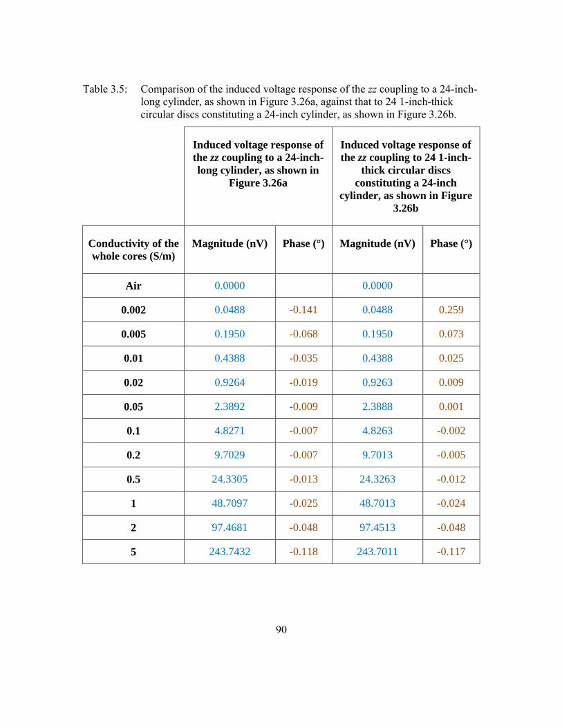
90

Table 3.5: Comparison of the induced voltage response of the zz coupling to a 24-inch-

long cylinder, as shown in Figure 3.26a, against that to 24 1-inch-thick

circular discs constituting a 24-inch cylinder, as shown in Figure 3.26b.

Induced voltage response of

the zz coupling to a 24-inch-

long cylinder, as shown in

Figure 3.26a

Induced voltage response of

the zz coupling to 24 1-inch-

thick circular discs

constituting a 24-inch

cylinder, as shown in Figure

3.26b

Conductivity of the

whole cores (S/m)

Magnitude (nV) Phase (°) Magnitude (nV) Phase (°)

Air 0.0000 0.0000

0.002 0.0488 -0.141 0.0488 0.259

0.005 0.1950 -0.068 0.1950 0.073

0.01 0.4388 -0.035 0.4388 0.025

0.02 0.9264 -0.019 0.9263 0.009

0.05 2.3892 -0.009 2.3888 0.001

0.1 4.8271 -0.007 4.8263 -0.002

0.2 9.7029 -0.007 9.7013 -0.005

0.5 24.3305 -0.013 24.3263 -0.012

1 48.7097 -0.025 48.7013 -0.024

2 97.4681 -0.048 97.4513 -0.048

5 243.7432 -0.118 243.7011 -0.117

91

Table 3.6: Induced voltage response of the zz coupling to a 1-inch-thick circular disc

for various values of conductivity of the disc and for various locations.

Induced voltage response of zz coupling (nV)

Location of the 1-inch-

thick circular disc (in.)

0.01-S/m

conductivity

disc

0.1-S/m

conductivity

disc

1-S/m

conductivity

disc

-12 0.00015 0.00171 0.01727

-11 0.00026 0.00291 0.02936

-10 0.00046 0.00513 0.05183

-9 0.00086 0.00946 0.09549

-8 0.00166 0.01824 0.1841

-7 0.00333 0.03663 0.3697

-6 0.00675 0.07433 0.75009

-5 0.01206 0.13273 1.33935

-4 0.00366 0.0403 0.4067

-3 -0.06103 -0.67129 -6.77386

-2 -0.12232 -1.34554 -13.57767

-1 -0.18612 -2.04733 -20.65936

0 -0.08316 -0.91469 -9.23005

1 0.17339 1.90731 19.24656

2 0.32299 3.55291 35.85213

3 0.24605 2.70661 27.3122

4 0.07662 0.84289 8.50559

5 0.02567 0.28244 2.85015

6 0.0097 0.10678 1.07752

7 0.00409 0.04498 0.45394

8 0.00188 0.02077 0.20957

9 0.00094 0.01034 0.10437

10 0.0005 0.00548 0.05532

11 0.00027 0.00306 0.03088

Sum of induced voltage

responses for various

locations of the disc

0.43866

4.82616

48.7017

Induced voltage response

of a 24-inch cylinder of

equivalent conductivity, as

mentioned in Table 3.5

0.4388

4.8271

48.7097

92

Table 3.7: Comparison of the estimated values of conductivity of individual layers with

and without the z-directed bucking coil for a whole core with random

distribution of 1-S/m and 0.01-S/m conductivity layers.

Layer #

(top to

bottom)

True

Conductivity

(S/m)

Estimated

conductivity,

without buck coil

(S/m)

Estimated

conductivity,

with buck coil

(S/m)

1 1 1.0068 1.0024

2 1 0.9989 1.0023

3 0.01 0.0168 0.0112

4 1 0.9998 1.0021

5 0.01 0.0111 0.011

6 0.01 0.0144 0.0109

7 0.01 0.008 0.0108

8 0.01 0.015 0.0107

9 1 1.0013 1.0016

10 0.01 0.0091 0.0105

11 1 1.0075 1.0014

12 1 0.9953 1.0013

13 0.01 0.0188 0.0102

14 0.01 0.0062 0.0101

15 1 1.0038 1.001

16 0.01 0.0101 0.0099

17 0.01 0.0084 0.0098

18 0.01 0.0147 0.0097

19 0.01 0.0048 0.0096

20 0.01 0.0164 0.0095

21 0.01 0.0041 0.0094

22 1 1.0052 1.0003

23 1 0.9973 1.0002

24 0.01 0.0124 0.0091

93

Figure 3.1: Comparison of the measured values against the SA model predictions of the

WCEMIT impedance response at 58.5 kHz to a TTL at 0°-azimuthal

orientation for various positions of the TTL along the tool axis.

-8 -4 0 4 8-4

0

4x 10

-3 (a) xx

-8 -4 0 4 8-1

0

1x 10

-3 (b) xy

-8 -4 0 4 8-0.01

0

0.01(c) xz

WCEMIT

SA

-8 -4 0 4 8-1

0

1x 10

-3 (d) yx

Imp

ed

an

ce

(

)

-8 -4 0 4 8-1

0

1x 10

-3 (e) yy

-8 -4 0 4 8-0.01

0

0.01(f) yz

-8 -4 0 4 8-0.01

0

0.01(g) zx

-8 -4 0 4 8-0.01

0

0.01(h) zy

Test loop position (in.)-8 -4 0 4 8

-0.04

-0.02

0(i) zz

94

Figure 3.2: Comparison of the measured values against the SA model predictions of the

WCEMIT impedance response at 58.5 kHz to a TTL at 45°-azimuthal

orientation for various positions of the TTL along the tool axis.

-8 -4 0 4 8-1

0

1x 10

-3 (a) xx

-8 -4 0 4 8-1

0

1x 10

-3 (b) xy

-8 -4 0 4 8-0.01

0

0.01(c) xz

WCEMIT

SA

-8 -4 0 4 8-1

0

1x 10

-3 (d) yx

Imp

ed

an

ce

(

)

-8 -4 0 4 8-1

0

1x 10

-3 (e) yy

-8 -4 0 4 8-0.01

0

0.01(f) yz

-8 -4 0 4 8-0.01

0

0.01(g) zx

-8 -4 0 4 8-0.01

0

0.01(h) zy

Test loop position (in.)-8 -4 0 4 8

-0.04

-0.02

0(i) zz

95

Figure 3.3: Comparison of the apparent conductivity response of the WCEMIT xx, yy,

and zz couplings at 58.5 kHz against the conductivity response of Orion

conductivity meter to an isotropic cylindrical volume of brine for varying

values of conductivity of the brine, ranging from 5 mS/m to 5 S/m.

Figure 3.4: Frameworks of two synthetic bilaminar whole core samples of 0°-dip (left)

and 45°-dip (right), respectively.

100

101

102

103

100

101

102

103

orion

(mS/m)

W

CE

MIT

(m

S/m

)

Theory

XX

YY

ZZ

96


conductivity responses of the xx, yy, and zz couplings at 58.5 kHz to four 0°-

dip bilaminar synthetic cores of 𝜆c of 1, 2, 5, and 10, respectively.


conductivity responses of the xx, yy, zz, -xz, and -zx couplings at 58.5 kHz to

four 45°-dip, 0°-azimuth bilaminar synthetic cores of 𝜆c of 1, 2, 5, and 10,

respectively.

1 2 5 1010

100

(a) xx

(

mS

/m)

1 2 5 1010

100

(b) yy

c

1 2 5 1010

100

1000

(c) zz

SA

WCEMIT

1 2 5 1010

100

1000

(a) xx

1 2 5 101

10

100

(d) -xz

(

mS

/m) 1 2 5 10

10

100

1000(b) yy

1 2 5 101

10

100(e) -zx

c

1 2 5 1010

100

1000

(c) zz

SA

WCEMIT

97


conductivity responses of all nine couplings at 58.5 kHz to four 45°-dip,

60°-azimuth bilaminar synthetic cores of 𝜆c of 1, 2, 5, and 10, respectively.

1 2 5 10

100

1000(a) xx

1 2 5 101

10

100

(b) -xy

1 2 5 101

10

100

(c) -xz

1 2 5 101

10

100

(d) -yx

(

mS

/m)

1 2 5 10

100

1000(e) yy

1 2 5 1010

100

(f) yz

1 2 5 101

10

100

(g) -zx

1 2 5 101

10

100

(h) zy

c

1 2 5 1010

100

1000

(i) zz

SA

WCEMIT

98

Figure 3.8: Photograph of (a) side view and (b) top view of the 4-inch-diameter Berea

whole core sample. (c) Fully saturated Berea whole core samples stored in

7.64-S/m-conductivity brine. (d) Berea whole core sample placed inside the

WCEMIT conduit for the conductivity tensor measurement.

a

b

c

d

99

Figure 3.9: Convergence of the estimates of (a) error, (b) 𝜎hor, (c) 𝜆c, and (d) θ during

the inversion of rotated conductivity tensor of the Berea whole core sample.


the inversion of rotated conductivity tensor of Boise whole core sample.

0 20 40 60 80 1000.001

0.01

0.1

1

10

Err

or

(a)

0 20 40 60 80 1000

1

2

3

4

hor (

S/m

)

(b)

0.752 S/m

0 20 40 60 80 1001

2

3

4

c

(c)

6.6461

1.01

0 20 40 60 80 1000

5

10

15

20

( )

Iteration #

(d)

2.86

0 20 40 60 800.001

0.01

0.1

1

10

Err

or

(a)

0 20 40 60 800

1

2

3

4

hor (

S/m

)

(b)

0.870 S/m

0 20 40 60 801

2

3

4

c

(c)

1.15

0 20 40 60 800

5

10

15

20

( )

Iteration #

(d)

2.86

100

Figure 3.11: Side view of the three 2-feet-long, 4-inch-diameter brine-filled glass-bead

packs made of (a) 6-mm, (b) 1.15-mm, and (c) 0.25-mm-diameter glass

beads that are referred to as Pack-1, Pack-2, and Pack-3, respectively.

Figure 3.12: Relationship of the true conductivity (σt) of brine-saturated glass-bead packs

made of 6-mm-diameter glass beads and pore-filling brine conductivity (σw).

Theoretical predictions based on the Archie’s equation are plotted for the

porosity exponent (m) values of 1.3, 1.33, and 1.38.

1000 1500 2000 2500 3000200

300

400

500

600

700

800

w

(mS/m)

t (

mS

/m)

Theory m=1.3

Theory m=1.33

Theory m=1.38

WCEMIT

a

b

c

101

Figure 3.13: Relationship of the formation factor (F) of brine-saturated glass-bead packs

and the brine-filled total porosity (𝜙tot). Theoretical predictions based on

the Archie’s equation are plotted for porosity exponent (m) values of 1.3,

1.33, and 1.38.

Figure 3.14: Side view of 2-feet-long, 4-inch-diameter brine-filled bilaminar glass-bead

packs: (a) Pack-6 and (b) Pack-7.

10-0.7

10-0.6

10-0.5

100.6

100.7

100.8

100.9

tot

F

Theory m=1.3

Theory m=1.33

Theory m=1.38

WCEMIT

b

a

102

Figure 3.15: Top view of 4-inch-diameter brine-filled glass-bead pack identifying vuggy

isotropic whole core. Uniformly distributed 6-mm glass beads identify non-

conductive vugs, and the remaining brine-filled volume made of 1.15-mm-

diameter glass beads identifies the fluid-saturated porous matrix.

Figure 3.16: Comparative plot of deviation of the formation factor (Fmod) of glass-bead

packs containing conductive (green curve) or non-conductive (blue curve)

vugs from the Archie’s formation factor (F) of packs containing no vugs

(dashed line) for various values of total porosity (𝜙tot) of the mixture. 𝜙tot

includes inter-granular porosity (𝜙h) and isolated vuggy porosity (𝜙i). The

value of 𝜙tot at which blue and green curves deviate from the black line

indicates the 𝜙h of the pack, and 𝜙t − 𝜙h indicates the vuggy porosity of

the pack.

10-1

100

100

101

102

tot

Fm

od

Non-conductive vugs

Conductive vugs

No vugs

WCEMIT

103

Figure 3.17: (a) A 2-feet-long, 4-inch-diameter synthetic whole core comprising 0.25-

inch TIVAR elliptical discs separated by 0.75 inches and oriented at 45°-

dip. (b) Schematic of such a whole core.

Figure 3.18: The cost functional as a function of angle of rotation of the complex

conductivity tensor.

0 60 120 180 240 300 3600

20

40

60

80

100

120

140

160

Angle of rotation ()

Co

st

fun

cti

on

al

(mS

/m)

104


inversion of the rotated conductivity tensor of 45°-dipping bilaminar

TIVAR-brine synthetic core.

Figure 3.20: SA model predictions of the WCEMIT R-signal response of yy-coupling to a

cylindrical volume of 𝜎hor of 1 S/m, 𝜆p of 1, and 휀r,hor of 1 for various

values of conductivity anisotropy ratio (𝜆c) of the cylindrical volume.

0 50 100 1500.001

0.01

0.1

1

10

Err

or

(a)

0 50 100 1500

2

4

6

hor (

S/m

)

(b)

0.886

0 50 100 1500

5

10

15

c

(c)

6.65

0 50 100 1500

20

40

60

( )

Iteration #

(d)

45.62

101

102

10-2

10-1

100

Frequency (kHz)

R-s

ign

al

(S/m

)

c=1

c=2

c=5

c=10

105

Figure 3.21: SA model predictions of the (a) R-signal and (b) X-signal responses of the

yy-coupling to a cylindrical volume of 𝜎hor of 1 S/m, 𝜆c of 1, and 휀r,hor of

105 for various values of 𝜆p of the cylindrical volume.


zz-coupling to a cylindrical volume of 𝜎hor of 1 S/m, 𝜆c of 1, 𝜆p of 1, and

휀r,hor of 105 for various values of dielectric loss factor (δ).

101

102

1

2

3

4

Frequency (kHz)

R-s

ign

al

(S/m

)

(a)

p=0.2

p=0.5

p=1

p=2

p=5

101

102

-2.5

-2

-1.5

-1

-0.5

0

Frequency (kHz)

X-s

ign

al

(S/m

)

(b)

101

102

1

1.5

2

2.5

Frequency (KHz)

R-s

ign

al

(S/m

)

(a)

101

102

-1.5

-1

-0.5

0

Frequency (KHz)

X-s

ign

al

(S/m

)

(b)

tan()=1

tan()=0.1

tan()=0.01

106


zz-coupling to an isotropic cylindrical volume of 𝜎hor of 1 S/m, 𝜆c of 1, 𝜆p

of 1, 휀r,s of 106, and α of 0.15 for various values of τ (s).



of 1, τ of 10-5 s, and α of 0.15 for various values of 휀r,s.

101

102

1

1.5

2

2.5

3

3.5

Frequency (kHz)

R-s

ign

al

(S/m

)

(a)

= 510-6

= 110-5

= 210-5

= 110-4

101

102

-1

-0.8

-0.6

-0.4

-0.2

0

Frequency (kHz)

X-s

ign

al

(S/m

)

(b)

101

102

1

1.5

2

2.5

Frequency (kHz)

R-s

ign

al

(S/m

)

(a)

r,s

= 106

r,s

= 5105

r,s

= 105

r,s

= 104

101

102

-0.5

-0.4

-0.3

-0.2

-0.1

0

Frequency (kHz)

X-s

ign

al

(S/m

)

(b)

107



of 1, τ of 10-5 s, and 휀r,s of 106 for various values of α.

Figure 3.26: (a) A 24-inch-long cylinder placed coaxially inside the coaxial z-directed

transmitter, receiver, and bucking coils (schematic representation). (b) 24 1-

inch-thick, juxtaposed, circular discs that are placed coaxially inside the

transmitter, receiver, and bucking coils to constitute a 24-inch-long cylinder.

101

102

1.3

1.5

1.7

1.9

2.1

2.3

2.5

Frequency (kHz)

R-s

ign

al

(S/m

)

(a)

= 0.15

= 0.05

= 0.25

101

102

-0.9

-0.7

-0.5

-0.3

-0.1

Frequency (kHz)

X-s

ign

al

(S/m

)

(b)

b a

108

Figure 3.27: Induced voltage response of the zz coupling to 1-inch-thick 0°-dip coaxial

circular disc located at various distance from z=0.

Figure 3.28: (a) A CT scan and UV fluorescence image of a whole core from a turbidite

reservoir comprising sand, shale, and cemented layers. (b) A conductivity

model of the turbiditic whole core for purposes of computing the whole core

logging measurements.

-15 -10 -5 0 5 10 1510

-4

10-2

100

102

104

Location of 1-inch-thick disc (in.)

Ind

uced

vo

ltag

e r

esp

on

se (

nV

)

0.01 S/m

0.1 S/m

1 S/m

10 S/m

b a

109

Figure 3.29: Modeled induced voltage response to synthetic whole core shown in Figure

3.28b as the whole core is coaxially translated from -11 to +32 inches.

Figure 3.30: Convergence of the estimates of (a) error and (b) 𝜎 of each layer during

inversion of the whole core logging measurements on synthetic whole core

shown in Figure 3.28b.

-15 -10 -5 0 5 10 15 20 25 30 35-60

-40

-20

0

20

40

60

80

Location of whole core (in.)

Ind

uced

vo

ltag

e r

esp

on

se (

nV

)

0 50 100 150 200 2500.1

1

10

100

1000

Err

or

(a)

0 50 100 150 200 2500.001

0.01

0.1

1

10

(

S/m

)

Iteration #

(b)

0.01 S/m

0.4 S/m

1 S/m

110

Figure 3.31: Comparison of estimated conductivity of the synthetic model of the

turbiditic sequence in Figure 3.28b with the true conductivity of each layer.

10-2

10-1

100

0

5

10

15

20

25

(S/m)

Co

re l

en

gth

(in

.)

Estimated

Original

111

Chapter 4: Effective Electrical Conductivity and Dielectric Permittivity

of Samples Containing Disseminated Mineral Inclusions

Organic-rich mudrock and source-rock formations generally contain electrically

conductive pyrite and graphitic-precursor mineralization in the form of veins, laminations,

flakes, and grains. In redox-inactive subsurface conditions, when an external

electromagnetic (EM) field is applied to geomaterials containing conductive mineral

inclusions, ions in the pore-filling brine and charge carriers in the electrically conductive

mineral inclusions, namely electrons and holes, accumulate/deplete at impermeable host-

inclusion interfaces giving rise to perfectly-polarized interfacial polarization (PPIP)

phenomena (explained in detail in Chapter 5). Such polarization phenomena influence the

diffusion, accumulation, and migration of charge carriers in a geomaterial; thereby, altering

its effective electrical conductivity (σeff) and effective relative dielectric permittivity (εr,eff).

In addition, the relaxation process associated with the interfacial polarization phenomena

and the time required to fully develop the field-induced polarization give rise to the

frequency dispersive σeff and εr,eff of mudrocks and source rocks containing pyrite and

graphitic-precursor inclusions. I investigate the effects of the PPIP phenomena exhibited

by pyrite-bearing and graphite-bearing samples on their directional and frequency

dispersive electrical properties. To that end, I first use the WCEMIT to measure the

directional multifrequency EM response of 4-inch-diameter, 2-ft-long glass-bead packs

containing uniformly distributed pyrite and graphite inclusions. The semi-analytic EM

forward model (SA Model) was then implemented to estimate the σeff and εr,eff of the

conductive-mineral-bearing glass-bead packs. I observe significant frequency dispersion

of the estimated electrical properties, large values of effective relative permittivity, and

significant alteration in the effective conductivity due to the variation in volume content

112

and size of conductive mineral inclusions. Also, conductive-mineral-bearing packs exhibit

conductivity anisotropy and permittivity anisotropy due to the effects of polarization of the

disseminated mineral inclusions.

4.1 INTRODUCTION

Organic-rich mudrocks and source-rock formations containing conductive mineral

inclusions, clay minerals, and clay-sized particles exhibit frequency dispersive effective

electrical conductivity and large effective dielectric permittivity in the EM induction

frequency range due to the interfacial polarization phenomena at host-inclusion interfaces.

The interfacial polarization phenomena significantly influence charge-carrier migration,

accumulation, and diffusion processes (Schmuck and Bazant, 2012; Wong, 1979).

Anderson et al. (2006), Wang and Poppitt (2013), and Misra et al. (2015d) mentioned that

limited laboratory and numerical modeling work has been published on the effects of

interfacial polarization of electrically conductive inclusions on subsurface galvanic, EM

induction, and EM propagation measurements. Conventional resistivity interpretation

methods typically give rise to inaccurate results in pyrite-bearing sedimentary formations

(Altman et al., 2008), pyrite-bearing mudrocks (Kethireddy et al., 2014), and pyrite-bearing

and graphitic-precursor-bearing source-rock formations (Anderson et al., 2008).

Passey et al. (2010) mentioned the challenges in resistivity interpretation due to the

presence of conductive pyrite and graphitic-precursor inclusions in source-rock formations

and shale gas reservoirs. Witkowsky et al. (2012) emphasized that there is a linear

correlation of the total organic content (TOC) and pyrite content, and resistivity

measurements should be corrected for the effects of pyrite content prior to using resistivity

measurements in the delta logR method. Recently, Chen and Heidari (2014) showed that

113

the directional dielectric permittivity estimation is strongly affected by the presence and

connectivity of mature organic matter and pyrite inclusions.

Clavier et al. (1976) measured the effect of pyrite inclusions on various resistivity

logging measurements. They observed a strong dependence of the resistivity measurements

on the distribution of pyrite inclusions and operating frequency of the logging tool. Despite

the absence of electrical connectivity of the pyrite phase, an increase in frequency of

electrical measurements led to an increase in electrical conductivity of the mixture. Clavier

et al. (1976) also showed that the frequency dispersion of conductivity response of a pyrite-

bearing mixture depends on the operating frequency, pyrite volume fraction, and pore-

filling brine salinity. Recently, Clennell et al. (2010) observed that the disseminated pyrite

inclusions in sandstones resulted in a drastic decrease in resistivity when pyrite content

exceeded 5% volume fraction. They used the Hanai-Bruggeman equation in the 1 Hz to

100 kHz frequency range to model the experimentally-measured effective conductivity and

dielectric permittivity response of sandstones containing disseminated pyrite grains.

However, Clennell et al. (2010) neglected the effects of interfacial polarization of pyrite

inclusions. More recently, Yu et al. (2014) showed that both the laboratory and downhole

measurements in high TOC marine shale formations exhibited frequency dispersion of the

0.1 Hz to 10 kHz frequency range due to the presence of pyrite inclusions of weight fraction

in the range of 1 to 5 wt%. They suggested that the implementation of a complex resistivity

method could improve resistivity interpretations in marine shale gas formations. Further,

they used the empirical dual Cole-Cole model (instead of a mechanistic formulation) to

analyze their data.

Al Duhailan et al. (2014) observed anomalous reversal in resistivity-thermal

maturity relationship in Niobrara formation when the formation changes from wet-gas

114

window to dry-gas window. They explained the decrease in resistivity as a consequence of

the change in wettability of the formation from oil-wet to water-wet state with the over-

maturation of the organic-rich source rocks. However, I propose that the generation of

graphitic-carbon (carbonization) during kerogen maturation as the reason for the reduction

in resistivity of organic-rich mudrocks and source rocks with the maturation of the

interstitial kerogen. Walters et al. (2014) performed high resolution transmission electronic

microscopy (HRTEM) experiments on shales of thermal maturity in the range of 0.6 to

>4.5%Ro. They found isolated turbostatic carbon nanostructures whose volume content

increased with increase in the maturity of the shale rock. Also, the presence of such carbon

nanostructures corresponded to the mature zones exhibiting anomalously high electrical

conductivity in the well logs. They concluded that the frequency of occurrence of carbon

nanostructures correlated with the abundance of organic carbon, its maturity, and

macroscopic electrical conductivity. Also, Romero-Sarmiento et al. (2014) performed

HRTEM experiments on powdered Barnett shale rocks and isolated kerogen samples. The

HRTEM-generated images showed nanoscale polyaromatic layers and carbon

nanostructures in mature organic-rich shale rock samples.

Since 1980s, the generation of graphitic-carbon due to carbonization and/or

graphitization of kerogen has been experimentally observed when kerogen is synthetically

matured by increasing the applied temperature and pressure (Spötl et al., 1998). Al Duba

(1983) performed laboratory-maturation experiments on Green River Shale rocks. He

observed that the initial bulk conductivity of 10-7 S/m started increasing around 400 °C,

which corresponded to the onset of hydrocarbon generation and aromatization of the

residual kerogen. The bulk conductivity reached a maximum conductivity value of 10 S/m

at 700 °C, which was attributed to the graphitic-precursor generated during the maturation

115

process. Recently, Buseck and Beyssac (2013) mentioned that the graphitic-precursor can

be used for geothermometry to quantify low-grade metamorphism (330 °C). They showed

that the graphitization of organic matter resulted in wide variety of intimately mixed

conductive structures that exhibit microporous, ring, lamellar, and planar nanostructures.

Allan et al. (2013) observed 82% decrease in resistivity measurements on organic-rich

shale rocks upon thermal maturation to the wet-gas window. The baseline resistivity

measurements of those rocks before the maturation were extremely high, in the order of

20000 ohm-m, because of the lack of connected conductive pore fluid. Consequently, Allan

et al. (2013) attributed the decrease in the resistivity measurements with maturation to the

carbonization of the kerogen and the conversion of smectite to illite.

The primary objective of this Chapter is to describe the effects of interfacial

polarization of conductive mineral inclusions on the EM response of WCEMIT in the EM

induction frequency range of 10 kHz to 300 kHz. WCEMIT allows non-contact,

directional, multi-frequency, inductive-complex conductivity measurements on whole core

samples containing pyrite and/or graphite inclusions. I analyze the WCEMIT

measurements (R- and X-signal responses) using the SA model, introduced in Chapter 2.

In doing so, I estimate εr,eff and σeff of the conductive-mineral-bearing glass-bead packs. I

also compare the measured responses and estimated values of electrical properties of the

packs containing graphite inclusions with those containing pyrite inclusions. This

comparison can facilitate discrimination of pyrite and graphite based on the WCEMIT

response. Finally, I study the WCEMIT response to layered glass-bead packs having layers

containing pyrite or graphite inclusions alternating with uncontaminated layers. This study

will test the accuracy of laminated shale sand analysis in layered formations, wherein some

layers exhibit high dielectric permittivity and frequency dispersive electrical properties.

116

4.2 MATERIALS AND METHODS

Two 4-inch-outer-diameter, 3.8-inch-inner-diameter, 2-ft-long cylindrical glass

vases were used to prepare the glass-bead packs. An inclusion-free glass-bead pack (Figure

4.1a) was prepared by filling the glass vase with 575-µm-radius glass beads and then fully

saturating the pore spaces between the glass beads with 3.75-S/m-conductivity brine. A

conductive-mineral-bearing pack (Figures 4.1b and 4.1c) was prepared by filling the glass

vase with a mixture of 575-µm-radius glass beads and conductive mineral inclusions of a

particular size to obtain a 2-inch thick layer. Following that, 3.75-S/m-conductivity brine

is poured into the glass vase to fully saturate the 2-inch thick layer. The vase was then

vibrated using a mechanical hand-held shaker to consolidate the mixture, remove trapped

air bubbles, and uniformly distribute the pore-filling brine. The three above-mentioned

steps were repeated until the entire glass vase was tightly-filled with glass beads,

inclusions, and brine. I consistently prepared 2-ft-long glass-bead packs having brine-filled

porosity of approximately 38%. Two sizes of nearly-spherical pyrite inclusions were used

for this study, namely the Pyrite Red (average diameter = 50 µm) and Pyrite Yellow

(average diameter = 130 µm) grains manufactured by Washington Mills

(http://www.washingtonmills.com/products/iron-pyrite/). Two sizes of flaky graphite

inclusions were used in this work, namely the #2 flake graphite (50×200 mesh size, average

surface area = 0.02 mm2) and the #1 flake graphite (50×80 mesh size, average surface area

= 0.06 mm2) manufactured by Dixon Graphite. The glass beads used in this work are 1.15-

mm-diameter Megalux beads manufactured by Swarco Company

(http://www.swarco.com/en/Products-Services/Traffic-Materials/Glass-Beads).

Multi-frequency inductive-complex conductivity measurements were obtained

with the WCEMIT, described in Chapter 2. The WCEMIT operates at seven frequencies

117

in the frequency range of 10 kHz to 300 kHz. The WCEMIT measurements on the

conductive-mineral-bearing glass-bead packs were inverted using the SA model to obtain

the εr,eff and σeff. Prior to performing the WCEMIT measurements on conductive-mineral-

bearing glass-bead packs, the WCEMIT system was calibrated for each of the seven

operating frequencies and for each of the nine transmitter-receiver coupling using the

tilted-test loop method, as described in Chapter 3. Following that, the directional

conductivity measurements were performed on the brine samples of known conductivity

for each of the seven operating frequencies, as described in Chapter 3. After the WCEMIT

calibration, the brine-saturated inclusion-free glass-bead pack (Figure 1a) was measured to

record the variations in the R- and X-signal responses of each of the nine transmitter-

receiver couplings at each of the seven operating frequencies. This frequency-dependent

variations in the R- and X- signal responses to the inclusion-free glass-bead packs are

associated with the undesirable polarization of glass beads and the vase, and is also

associated with the frequency-dependent magnitude and phase changes due to the

peripheral electronics of the system. These variations in the R- and X-signal responses of

each of the nine couplings at the seven operating frequencies were used for the final gain

corrections on subsequent measurements of R- and X-signal responses to glass-bead packs

containing inclusions.

In the laboratory, one can measure weights of the inclusion and host phases more

accurately than their volumes because the volume measurements require correction for the

volume occupied by air. Measured weights are converted to volumes using the measured

densities of the host and inclusion phases to obtain the volume fraction of the inclusion

phase. I present my laboratory results as a function of the volume fraction of the inclusion

phase to enable petrophysicists and geoscientists to better correlate the results of my

118

findings with subsurface and laboratory measurements, which are generally carried out as

a function of the volume fraction. I measured that 308.65 g of the air-filled unconsolidated

pack of glass beads occupied 210 cm3, and the density of the air-filled unconsolidated pack

of glass beads is 1.47 g/cm3 (bulk density), while that of only the glass beads is 2.37 g/cc

(density), assuming 40% air-filled porosity of the glass-bead packs. These values are in the

range of the bulk density of 1.2 to 1.8 g/cc and that of the density of 2.2 to 2.6 g/cc of the

Megalux Beads as reported in the Swarco Safety Data Sheet (2004). I also measured that

15 g of air-filled unconsolidated pack of graphite flake #2 occupied 20 cm3, which amounts

to a density of 0.75 g/cm3 of the air-filled unconsolidated pack of graphite flake #2. This

value is in agreement with the bulk density of graphite flakes as reported in several

publications (e.g., Franklin Miller Inc., 2015). Further, I measured that 93 g of the air-filled

unconsolidated pack of Pyrite Red particles occupied 68 cm3, which amounts to a density

of 1.37 g/cm3 of the air-filled unconsolidated pack of Pyrite Red particles. This value is in

agreement with the bulk density of pyrite powder as reported in several publications (e.g.,

Ken and Stewart, 1999).

4.3 EFFECTS OF UNIFORMLY DISTRIBUTED PYRITE INCLUSIONS

4.3.1 R- and X-signal responses

Using the WCEMIT system, I first measured the R- and X-signal responses of the

zz (Figure 4.2) and yy (Figure 4.3) couplings to the glass-bead packs containing uniformly

distributed Pyrite Red inclusions for volume fractions of the inclusion phase of 0.5%, 1.5%,

2.5%, and 5%. In Figures 4.2 and 4.3, the frequency dispersions of the R- and X-signal

responses increase with an increase in the volume fraction of Pyrite Red inclusions because

the difference between the static and high-frequency limits of effective conductivity and

119

relative permittivity increases with increase in the volume content of pyrite inclusions. As

observed in many subsurface EM tool measurements (e.g., Anderson et al., 2006; Wang

and Poppitt, 2013), large negative X-signal responses were measured for the pyrite-bearing

glass-bead packs, which indicates that the presence of pyrite inclusions gives rise to a

substantial dielectric permittivity associated with the interfacial polarization phenomena.

Notably, the R- and X-signal responses obtained for the yy coupling (Figure 4.3) are

distinct from those obtained for the zz coupling (Figure 4.2), implying that the pyrite-

bearing glass-bead packs possess both conductivity and permittivity anisotropy. R-signal

response mostly decreases, while the negative X-signal response increases in magnitude

with an increase in the volume fraction of the inclusion phase.

Using the WCEMIT system, I also measured the R- and X-signal responses of the

zz (Figure 4.4) and yy (Figure 4.5) couplings to the glass-bead packs containing uniformly

distributed Pyrite Red (average radius = 25 µm) or Pyrite Yellow (average radius = 65 µm)

inclusions for volume fractions of the inclusion phase of 1.5% and 5%. In Figures 4.4 and

4.5, the frequency dispersions of R- and X-signal responses increase with an increase in

the size of pyrite inclusions because larger-sized conductive inclusions fail to fully polarize

at much low frequencies compared to smaller-sized conductive inclusions. Glass-bead

packs containing larger-diameter Pyrite Yellow inclusions exhibit a peak in X-signal

response of the zz coupling (Figure 4.4b). Both R- and X-signal responses mostly increase

with an increase in the size of inclusion phase.

The sensitivity of the R-signal responses of the yy and zz couplings to the variations

in size and volume fraction of pyrite inclusions in the glass-bead packs decreases, while

that of the negative X-signal responses of the yy and zz couplings increases in magnitude

with an increase in the operating frequency. At an operating frequency of 58.5 kHz, the

120

presence of 1.5% volume fraction of pyrite inclusions in the glass-bead packs resulted in

approximately 5% decrease in the R-signal response with respect to the R-signal response

to inclusion-free glass-bead pack, and produced an X-signal response of approximately -

25 mS/m. Further, at an operating frequency of 58.5 kHz and at a volume fraction of 1.5%

of pyrite inclusions in the glass-bead packs, a 160% increase in the size of the inclusions

from 25 µm to 65 µm, resulted in a 3% increase in the R-signal response and a 50% increase

in the magnitude of the negative X-signal response.

4.3.2 Directional effective electrical conductivity and relative dielectric permittivity

Frequency-dependent horizontal and vertical effective electrical properties of the

pyrite-bearing glass-bead packs are estimated by tweaking the SA model input values of

conductivity and relative permittivity to obtain the best match of the SA model predictions

to the multi-frequency zz coupling response and to the multi-frequency yy coupling

response, respectively. Figures 4.6 and 4.7 show the frequency dispersions of both the σeff

and εr,eff of the pyrite-bearing packs. The estimated values of εr,eff of the pyrite-bearing

packs are in the order of 103 to 104, which are similar to the large permittivity values

estimated by Anderson et al. (2006) and Wang and Poppitt (2013). Further, the vertical

values of σeff and εr,eff are less dispersive than the horizontal values. Interestingly, for low

operating frequencies, the σeff of the pyrite-bearing packs decreased with an increase in the

volume fraction of the pyrite inclusions, which indicates that the pyrite inclusions are

acting as non-conductive particles. However, for higher operating frequencies, the pyrite

inclusions act as conductive particles giving rise to an increase in the σeff with an increase

in the pyrite content. The counter-intuitive behavior of the σeff of the pyrite-bearing glass-

bead packs containing pyrite inclusions with respect to operating frequency can be

explained on the basis of perfectly-polarized interfacial polarization of pyrite inclusions

121

(Misra et al., 2015c; Revil et al., 2015) due to which conductive inclusions behave as non-

conductive particles at very low frequencies and as highly-conductive particles at high

frequencies.

Figures 4.8 and 4.9 depict the estimated horizontal and vertical σeff and εr,eff of the

glass-bead packs containing disseminated Pyrite Red (average radius = 25 µm) or Pyrite

Yellow (average radius = 65 µm) inclusions for volume fraction of the inclusion phase of

1.5% and 5%. In Figures 4.8 and 4.9, the frequency dispersions of σeff and εr,eff of pyrite-

bearing packs is larger for packs containing Pyrite Yellow inclusions than that containing

Pyrite Red inclusions because larger-sized conductive inclusions fail to fully polarize at

lower frequencies compared to smaller-sized conductive inclusions; thereby exhibiting

frequency dispersion at lower operating frequencies.

For operating frequencies around 58.5 kHz or lower, the σeff and εr,eff of pyrite-

bearing glass-bead packs made of 25-µm pyrite inclusions are close to the static limits as

predicted by Maxwell-Garnett effective medium model. Importantly, the effects of

interfacial polarization of 25-µm pyrite inclusions on the accuracy of estimation of σeff

based on Maxwell-Garnett effective medium model is negligible for operating frequencies

around 58.5 kHz or lower. Comparison of Figures 4.6 and 4.7 indicates that the frequency

dispersion effects of interfacial polarization of 25-µm pyrite inclusions are lower in the

vertical direction than that in the horizontal direction. A probable explanation of that

behavior is that there is a greater reduction in the surface area of pyrite inclusions

susceptible to interfacial polarization in the vertical direction compared to that in the

horizontal direction due to the tighter packing under gravity in the vertical direction that

results in increased contact of pyrite inclusions with adjacent glass beads in the vertical

direction. Notably, the effects of interfacial polarization of 5%-volume-fraction of 65-µm

122

pyrite inclusions on the accuracy of estimation of σeff based on Maxwell-Garnett effective

medium model is non-negligible for operating frequencies around 58.5 kHz or lower. The

effects of interfacial polarization on the σeff and εr,eff of pyrite-bearing glass-bead packs in

the EM induction frequency range increases with an increase in the volumetric content and

size of the pyrite inclusions.

4.3.3 Conductivity and permittivity anisotropy ratio

Based on the results shown in Figures 4.6, 4.7, 4.8, and 4.9, pyrite-bearing glass-

bead packs exhibit both effective conductivity and permittivity anisotropy. In Figure 4.10,

conductivity anisotropy ratio (λc) of the pyrite-bearing packs increase, while effective

permittivity anisotropy ratio (λp) decrease with an increase in operating frequency. These

trends in λc and λp are attributed to the frequency dispersion behavior of σeff, which

increases with an increase in operating frequency, and that of εr,eff, which decreases with

an increase in the operating frequency. Further, the sensitivity of λp to variations in volume

fraction of pyrite inclusions is negligible, while that of λc strongly depends on the volume

fraction of pyrite inclusions, as illustrated in Figure 4.10. However, the frequency

dependence of λp of pyrite-bearing packs is larger compared to that of λc, wherein λc is in

the range of 1 to 1.2, and λp is in the range of 1.7 to 2.8.

Figure 4.11 compares λc and λp of pyrite-bearing packs containing uniformly

distributed Pyrite Red (25 µm) against those containing uniformly distributed Pyrite

Yellow (65 µm) inclusions for volume fraction of the inclusion phase of 1.5% and 5%. An

increase in the size of pyrite inclusions increases the λc but decreases the λp. For operating

frequencies around 58.5 kHz or lower, a 160% increase in the size of the inclusions from

25 µm to 65 µm, resulted in a 9% increase in the λc and an 18% decrease in the λp.

Interestingly, I observe a peak in the λp for the packs containing Pyrite Yellow inclusions,

123

which can be attributed to the peak of relaxation time of the interfacial polarization of those

pyrite inclusions. The experimental results suggest that the values of λc are close to 1 and

their effects on resistivity interpretation can be neglected; however, the values of λp are

close to 2 and resistivity interpretation methods should account for possible effects of

permittivity anisotropy.

4.4 EFFECTS OF UNIFORMLY DISTRIBUTED GRAPHITE INCLUSIONS

4.4.1 R- and X-signal responses

Using the WCEMIT system, I first measured the R- and X-signal responses of the

zz and yy couplings to the glass-bead packs containing uniformly distributed #2 graphite

flake inclusions for volume fractions of the inclusion phase of 2%, 4%, 6%, and 10%. In

Figure 4.12, the frequency dispersions of the R- and X-signal responses increase with an

increase in the volume fraction of #2 graphite flake inclusions. The magnitude of the

negative X-signal responses of the graphite-bearing packs are much larger than that of the

pyrite-bearing packs. Notably, the R- and X-signal responses obtained for the yy coupling

(dotted) are distinct from those obtained for the zz coupling (solid), implying that the

graphite-bearing glass-bead packs possess both conductivity and permittivity anisotropy.

Unlike the R- and X-signal responses of packs containing pyrite inclusions, both the R-

signal response and the negative X-signal response increase in magnitude with an increase

in the volume fraction of the inclusion phase. This indicates that the graphite inclusions act

as conductive particles in the EM induction frequency range. Moreover, the difference in

R-signal response of packs containing pyrite inclusions from those containing graphite

inclusions highlight that the graphite inclusions have higher relaxation times compared to

those containing pyrite inclusions. Gurin et al. (2015) reported that graphite-bearing

124

samples have higher relaxation times compared to those of pyrite-bearing samples. For

volume fraction of 10% of graphite inclusions, the packs exhibit very large frequency-

dispersive R- and X-signal responses. However, such rocks containing volume fraction of

graphite more than 4% are not associated with productive hydrocarbon-bearing rocks.

Using the WCEMIT system, I also measured the R- and X-signal responses of the

zz (solid) and yy (dotted) couplings to the glass-bead packs containing uniformly

distributed #1 graphite flake inclusions. Figure 4.13 compares the response of a pack

containing #1 graphite flake inclusions (average surface area = 0.06 mm2) against that

containing #2 graphite flake inclusions (average surface area = 0.02 mm2) for the volume

fraction of the inclusion phase of 2%. The zz coupling exhibits larger sensitivity of the R-

signal response to the variation in the operating frequency compared to that of the yy

coupling, which is similar to that observed for pyrite-bearing packs. Further, at a given

volume fraction, the R-signal responses and the magnitude of the negative X-signal

responses of packs containing #2 graphite flake inclusions are larger compared to those

containing #1 graphite flake inclusions.

At an operating frequency of 58.5 kHz, the presence of 2% volume fraction of #2

graphite inclusions in the glass-bead packs resulted in approximately 20% increase in the

R-signal response with respect to the R-signal response to inclusion-free glass-bead pack,

and produced an X-signal response of approximately -150 mS/m. Further, at an operating

frequency of 58.5 kHz and at a volume fraction of 2% of graphite inclusions in the glass-

bead packs, a 200% increase in the surface area of the representative graphite inclusion

from 0.02 mm2 to 0.06 mm2, resulted in a 4% decrease in the R-signal response and a 12%

decrease in the magnitude of the negative X-signal response.

125

4.4.2 Effective electrical conductivity and relative dielectric permittivity

Frequency-dependent horizontal and vertical effective electrical properties of the

graphite-bearing glass-bead packs are estimated by tweaking the SA model input values of

conductivity and relative permittivity to obtain the best match of the SA model predictions

to the multi-frequency zz coupling response (solid) and to the multi-frequency yy coupling

response (dotted), respectively. Figure 4.14 shows the frequency dispersions of both the

σeff and εr,eff of the graphite-bearing packs. The estimated values of the εr,eff of the graphite-

bearing packs are in the order of 104 to 106, which are one to two order of magnitude higher

than those of pyrite-bearing packs. This indicates that the presence of graphite inclusions

gives rise to higher accumulation of charges compared to pyrite inclusions mostly due their

larger surface area. Owing to the higher diffusion coefficient (approximately around 10-3

m2s-1) and higher conductivity of graphite (105 S/m) than that compared to those of pyrite

of 10-6 m2s-1 and 103 S/m, respectively, the εr,eff and σeff values of the graphite-bearing

inclusions are much larger than that of pyrite-bearing packs (Revil et al., 2015a). Moreover,

a large dielectric loss factor is associated with such large εr,eff gives rise to the substantial

increase in the σeff. Further, the vertical values of σeff are less dispersive than the horizontal

values, similar to those of pyrite-bearing packs. However, both horizontal and vertical

values of the εr,eff have similar magnitude of frequency dispersion and exhibit a power-law

relationship with the operating frequency. Unlike the σeff of pyrite-bearing packs, the σeff

of the graphite-bearing packs increase with an increase in the volume fraction of the

graphite inclusions, which indicates that the graphite inclusions are acting as conductive

particles in the EM induction frequency range.

Figures 4.15 and 4.16 depict the estimated horizontal and vertical σeff and εr,eff of

the glass-bead packs containing disseminated #2 graphite flake inclusions (average surface

126

area = 0.02 mm2) and #1 graphite flake inclusions (average surface area = 0.06 mm2)

inclusions for volume fraction of the inclusion phase of 2% and 10%, respectively. In

Figures 4.15 and 4.16, the frequency dispersions of σeff and εr,eff of graphite-bearing packs

are similar for packs containing #2 graphite flake inclusions and those containing #1

graphite flake inclusions. Nonetheless, at any given operating frequency and volume

fraction of graphite inclusions, the packs containing #2 graphite flake inclusions show

higher values of εr,eff and σeff compared to those containing #1 graphite flake inclusions.

This behavior suggests that the packs containing #2 graphite flake inclusions produces

larger interfacial polarization effects than those containing #1 graphite flake inclusions.

For pyrite-bearing packs, increase in size of spherical pyrite inclusions shifted the

relaxation time to higher values; thereby increasing the values of εr,eff and σeff compared to

those containing smaller-sized inclusions. However, for graphite-bearing packs, an

increase in the size of a flaky graphite inclusion increases the surface area; thereby

increasing the εr,eff and the associated dielectric factor that increases the σeff. Also, the pack

containing #2 graphite inclusions and that containing #1 graphite inclusion exhibit a large

increase in the horizontal σeff at frequencies above 88 kHz.

For operating frequencies around 58.5 kHz or lower, the σeff of the glass-bead pack

containing 2% volume fraction of #2 graphite flake inclusions is 20% more than the host

conductivity, while that of the pack containing 10% volume fraction of #2 graphite flake

inclusions is 350% more than the host conductivity. These large differences in the values

of σeff compared to the host conductivity is attributed to the large dielectric loss factor

associated with the large vales of εr,eff of 5×104 and 5×105, respectively, that substantially

increases the σeff values. Importantly, the effects of interfacial polarization of #2 graphite

flake inclusions severely reduces the accuracy of estimation of σeff for operating

127

frequencies around 58.5 kHz or lower. Figures 4.15 and 4.16 indicate that the frequency

dispersion effects of interfacial polarization of #2 graphite flake inclusions are much lower

in the vertical direction than those in the horizontal direction, similar to the responses of

the pyrite-bearing packs. The effects of interfacial polarization of graphite inclusions on

the σeff and εr,eff of the graphite-bearing glass-bead packs in the EM induction frequency

range increases with an increase in the volumetric content and size of the graphite

inclusions.

4.4.3 Conductivity and permittivity anisotropy ratio

Based on the estimation of εr,eff and σeff, graphite-bearing packs exhibit both

effective conductivity and permittivity anisotropy. In Figure 4.17, λc values of the graphite-

bearing packs increase, while λp values decrease with an increase in the operating

frequency, similar to that of pyrite-bearing inclusions. Further, the sensitivity of λp and λc

to variations in volume fraction of graphite inclusions is non-negligible, unlike that

observed for pyrite-bearing packs. The frequency dependence of λp of graphite-bearing

packs is comparable to that of λc, wherein λc is in the range of 1 to 1.6 and λp is in the range

of 1 to 1.8. Graphite-bearing packs exhibit smaller values of εr,eff in the EM induction

frequency range compared to the pyrite-bearing packs.

Figure 4.17 also compares the λc and λp of graphite-bearing packs containing

uniformly distributed #2 graphite flakes against those containing uniformly distributed #1

graphite flakes for volume fraction of the inclusion phase of 2% and 10%. An increase in

the surface area of the representative graphite inclusion deceases both the λc and λp, which

is due to the increase in the randomness of the orientation of larger-sized inclusions. For

operating frequencies around 58.5 kHz or lower and volume fraction of 2%, a 200%

increase in the surface area of the representative graphite inclusion from 0.02 mm2 to 0.06

128

mm2, resulted in a 1% decrease in the λc and an 10% decrease in the λp. In my experiments,

at volume fractions of 2%, the values of λc and λp are close to 1, both λc and λp have low

sensitivity to variations in the size, volume fraction, and operating frequency.

4.5 EFFECTS OF PYRITE- AND GRAPHITE-BEARING LAYERS

In this section, I measure the WCEMIT response to bi-laminar glass-bead packs

that have alternating layers of different volume fractions of graphite (e.g., Figures 4.18a

and 4.18b) or pyrite inclusions (e.g., Figure 4.18c). Figure 4.19 compares the horizontal

and vertical σeff and εr,eff of a bi-laminar pack made of alternating 0-vol% and 10-vol% of

uniformly distributed #2 graphite-bearing layers (red) against those of two homogeneous

packs of 5-vol% and 10-vol%, respectively, of uniformly distributed #2 graphite

inclusions. In that figure, the horizontal and vertical σeff of the bi-laminar pack is

approximately 8% more, while the horizontal and vertical εr,eff is approximately 250% more

than those of the homogeneous 5-vol% graphite-bearing pack. Though the overall volume

fraction of graphite in the bi-laminar pack is equal to that of the homogeneous 5-vol%

graphite-bearing pack, Figure 4.19 indicates a large difference in their εr,eff values, which

can be attributed to the larger accumulation by the alternating 10-vol% graphite-inclusion-

bearing layers compared to that of the homogeneous, uniformly distributed 5-vol% of

graphite inclusions. Further, the horizontal and vertical εr,eff of the homogeneous 10-vol%

graphite-bearing pack is 300% more, whereas the horizontal and vertical σeff of the

homogeneous 10-vol% graphite-bearing pack is 200% more than those of the bi-laminar

pack. Notably, the bi-laminar pack shows no noticeable increase in the horizontal σeff for

operating frequencies higher than 88 kHz, as exhibited by the homogeneous 10-vol%

graphite-bearing pack.

129

Figure 4.20 compares the horizontal and vertical σeff and εr,eff of a bi-laminar pack

made of alternating 0-vol% and 10-vol% of uniformly distributed #1 graphite-bearing

layers (red) against those of a homogeneous pack of 10-vol% of uniformly distributed #1

graphite inclusions (green). Here, the bi-laminar pack exhibits a large increase in the

horizontal σeff for operating frequencies higher than 88 kHz, as exhibited by the

homogeneous 10-vol% graphite-bearing pack. Also, the values of horizontal σeff of the

bilaminar pack (red, solid) are 14% more than the values of effective horizontal

conductivity calculated using the series conductivity model for the 0-vol% and 10-vol%

graphite-inclusion-bearing layers (magenta, solid). Similarly, the values of horizontal εr,eff

of the bilaminar pack (red, solid) are 40% more than the values of effective horizontal

relative permittivity calculated using the series permittivity model for the 0-vol% and 10-

vol% graphite-inclusion-bearing layers (magenta, solid). Further, the values of vertical σeff

of the bi-laminar pack (red, dotted) are 23% more than the values of effective vertical

conductivity calculated using the parallel conductivity model for the 0-vol% and 10-vol%

graphite-inclusion-bearing layers (magenta, dotted). Although the series-parallel model is

not applicable for the bi-laminar pack because of the complex conductivity exhibited by

the bilaminar pack, the calculated values based on the series-parallel model is relatively

close to the estimated effective conductivity and permittivity values. Also, in Figure 4.20b,

the εr,eff values of the bilaminar pack in the horizontal direction are much larger than those

in the vertical direction, unlike the vertical and horizontal εr,eff values of the homogeneous

10-vol% graphite-bearing pack.

Figure 4.21 compares the horizontal and vertical σeff and εr,eff of a bi-laminar pack

made of alternating 0-vol% and 6-vol% of uniformly distributed #1 graphite-bearing layers

(red) against those of a homogeneous pack of 6-vol% of uniformly distributed #1 graphite

130

inclusions (green). Notably, the bi-laminar pack exhibits a large increase in the horizontal

σeff for operating frequencies higher than 88 kHz, as exhibited by the homogeneous 6-vol%

graphite-bearing pack. Also, the values of horizontal σeff of the bi-laminar pack (red, solid)

are 22% more than the values of effective horizontal conductivity calculated using the

series conductivity model for the 0-vol% and 6-vol% graphite-inclusion-bearing layers

(magenta, solid). Similarly, the values of horizontal εr,eff of the bi-laminar pack (red, solid)

are 43% more than the values of effective horizontal relative permittivity calculated using

the series permittivity model for the 0-vol% and 6-vol% graphite-inclusion-bearing layers

(magenta, solid). Further, the values of vertical σeff of the bi-laminar pack (red, dotted) are

16% more than the values of effective vertical conductivity calculated using the parallel

conductivity model for the 0-vol% and 6-vol% graphite-inclusion-bearing layers (magenta,

dotted). Also, in Figure 4.21b, the εr,eff values of the bi-laminar pack in the horizontal

direction (red, solid) are much larger than those in the vertical direction (red, dotted), unlike

the vertical and horizontal εr,eff values of the homogeneous 6-vol% graphite-bearing pack.

Therefore, a layered graphite-bearing pack exhibits large values of permittivity anisotropy

ratio.

Figure 4.22 shows that the bi-laminar pack containing alternating 0-vol% and 10-

vol% of uniformly distributed #1 graphite-bearing layers (blue) exhibits larger λc and λp

compared to the homogeneous 5-vol% #1 graphite-bearing pack (green). Although overall

the volume fraction of graphite inclusions is equal in both packs, both λc and λp are larger

for the bi-laminar pack. The increase λc in is negligible around an operating frequency of

58.5 kHz or lower; however, there is 120% increase in λp for those frequencies. This

observation confirms that the bi-laminar packs contribute to increase in permittivity

anisotropy in the pack.

131

4.6 COMPARISON OF THE EFFECTS OF UNIFORMLY DISTRIBUTED PYRITE-

BEARING PACKS AGAINST UNIFORMLY DISTRIBUTED GRAPHITE-BEARING PACKS

Several researchers have investigated the differences in the frequency dispersion of

conductivity and permittivity of samples containing graphite and pyrite inclusions (e.g.,

Gurin et al. 2015; Pelton et al., 1978) for purposes of mineral discrimination. Shale-gas

reservoirs are prone to the presence of graphitic-precursors and pyrite (Laughrey et al.,

2011; Passey et al., 2010). Therefore, in this section, I investigate qualitative differences

in the effective conductivity and permittivity of packs containing only graphite inclusions,

only pyrite inclusions, and mixture of graphite and pyrite inclusions.

Figure 4.23 compares the horizontal and vertical σeff and εr,eff of the graphite-

bearing pack (green) containing uniformly distributed 1.5-vol% of graphite inclusions

against those of pyrite-bearing pack (red) containing uniformly distributed 1.5-vol% of

pyrite inclusions. The σeff of the graphite-bearing pack is 16% more than that of the pyrite-

bearing packs. I observe that the presence of pyrite inclusions tends to decrease the σeff to

values below the host conductivity for various volume fractions of pyrite inclusions (Figure

4.6), while the presence of graphite inclusions tends to increase the σeff to values higher

than the host conductivity for various volume fractions of graphite inclusions (Figure 4.14).

Further, the εr,eff of the graphite-bearing pack is 400% more than that of the pyrite-bearing

pack. Moreover, the λc of the graphite-bearing pack is larger than that of the pyrite-bearing

pack that increases with an increase in the operating frequency, whereas the λp of pyrite-

bearing pack is larger than that of the graphite-bearing pack that decreases with a decrease

in the operating frequency.

Figure 4.24 compares the horizontal and vertical σeff and εr,eff of a graphite-bearing

pack (green) containing uniformly distributed 2-vol% of graphite inclusions, a pyrite-

bearing pack (red) containing uniformly distributed 2.5-vol% of pyrite inclusions, and

132

mixed-mineral-bearing pack containing uniformly distributed 2-vol% of graphite and 2.5-

vol% of pyrite inclusions (magenta). In that figure, the σeff values of the 2.5-vol% pyrite-

bearing pack are lower than the host conductivity (blue), whereas the 2-vol% graphite-

bearing pack exhibits a σeff value that is approximately 15% more than the host

conductivity. Notably, the mixed-mineral-bearing pack exhibits a value of σeff that is much

larger than the sum of the σeff values of the pyrite-bearing pack and graphite-bearing pack

for all the operating frequencies. Also, the mixed-mineral-bearing pack exhibits larger

values of λc compared to those of the pyrite-bearing pack and graphite-bearing pack that

increases with an increase in the operating frequency. Further, the mixed-mineral-bearing

pack exhibits horizontal and vertical εr,eff that is slightly more than the sum of the εr,eff

values of the pyrite-bearing pack and graphite-bearing pack. Comparison of the σeff and

εr,eff data indicate the non-additive nature of the effects of interfacial polarization of

different types of mineral inclusions.

Figure 4.25 compares the horizontal and vertical σeff and εr,eff of the mixed-mineral-

bearing pack containing uniformly distributed 5-vol% of #2 graphite inclusions and 2.5-

vol% of Pyrite Red inclusions (red) against those of the mixed-mineral-bearing pack

containing uniformly distributed 2-vol% of #1 graphite inclusions and 2.5-vol% of Pyrite

Red inclusions (magenta). In Figure 4.25, the mixed-mineral-bearing pack containing 7.5-

vol% of conductive mineral inclusions exhibited 30% increase in the horizontal σeff and

75% increase in the vertical εr,eff compared to those of the mixed-mineral-bearing pack

containing 4.5-vol% of conductive mineral inclusions. The packs containing only pyrite

inclusions have distinct σeff and εr,eff responses compared to the packs containing graphite

inclusions. Moreover, the packs containing both graphite and pyrite inclusions exhibit σeff

and εr,eff responses that are qualitatively similar to packs containing only graphite

133

inclusions, wherein the effects of pyrite inclusions are altered such that the effects of pyrite

inclusions on σeff and εr,eff are comparable to those of graphite inclusions.

4.7 CONCLUSIONS

Glass-bead packs containing homogeneously dispersed pyrite and/or graphite

inclusions exhibited frequency dispersion of their R- and X-signal responses due to the

interfacial polarization of electrically conductive mineral inclusions. The R-signal response

of conductive-mineral-bearing packs were significantly different from those of the

inclusion-free glass-bead packs; consequently, accurate resistivity interpretation methods

for samples containing pyrite or graphite inclusions must account for the effects of

interfacial polarization. Also, negative values of X-signal response were observed for

glass-bead packs containing more than 1%-volume-fraction of graphite or pyrite

inclusions, which is indicative of the dielectric behavior (charge accumulation) of these

packs due to the interfacial polarization phenomena. I successfully estimated the effective

conductivity and effective relative permittivity of the conductive-mineral-bearing glass-

bead packs using the Semi-Analytic EM forward model. The estimated values of the

effective relative permittivity were in the range of 103 to 104 for the pyrite-bearing glass-

bead packs and 104 to 106 for the graphite-bearing glass-bead packs. The effective electrical

conductivity and dielectric relative permittivity of the conductive-mineral-bearing packs

are strongly dependent on the operating frequency, mineral type, and volume fraction and

size of mineral inclusions. The multi-frequency effective conductivity and relative

permittivity of graphite-bearing packs were significantly different compared to those of the

pyrite-bearing packs due to the large difference in the diffusion coefficients of charge

carriers, bulk conductivity values, and shapes of pyrite and graphite inclusions. Further,

the packs containing homogeneously dispersed conductive inclusions exhibit conductivity

134

anisotropy ratios, in the range of 1 to 1.7, and permittivity anisotropy ratios, in the range

of 1.1 to 2.8. Consequently, resistivity interpretation methods for formations containing

uniformly dispersed pyrite or graphite inclusions must account for the effects of effective

conductivity and effective permittivity anisotropy due to interfacial polarization of the

inclusion phase. Notably, the packs containing alternating layers of different volume

fraction of conductive mineral inclusions have significantly different effective conductivity

and relative permittivity compared to those of packs containing homogeneously distributed

mineral inclusions of the same mineral type, size, total volume fraction, and shape.

Therefore, accurate resistivity interpretation in formations containing conductive minerals

will require accurate knowledge of shape, size, mineral type, conductivity, and distribution

of the inclusion phase.

Figure 4.1: Photographs of the 4-inch-diameter, 24-inch-long, glass-bead packs

containing (a) no inclusions, (b) 2.5% volume fraction of uniformly

distributed pyrite inclusions, and (c) 3-wt% of uniformly distributed

graphite inclusions fully saturated with 3.75-S/m-conductivity brine.

a b c

135


discrete points, of zz coupling to packs containing disseminated Pyrite Red

inclusions for various volume fractions of the inclusion phase. The dotted

curves identify SA model predictions that best fit the WCEMIT response.


discrete points, of yy coupling to packs containing disseminated Pyrite Red

inclusions for various volume fractions of the inclusion phase. The dotted

curves identify SA model predictions that best fit the WCEMIT response.

101

102

0.8

0.85

0.9

0.95

1

Frequency (kHz)

R-S

ign

al (S

/m)

(a)

101

102

-0.25

-0.2

-0.15

-0.1

-0.05

0

Frequency (kHz)

X-S

ign

al (S

/m)

(b)

0%

0.5%

1.5%

2.5%

5%

101

102

0.8

0.84

0.88

0.92

0.96

1

Frequency (kHz)

R-S

ign

al (S

/m)

(a)

101

102

-0.12

-0.08

-0.04

0

Frequency (kHz)

X-S

ign

al (S

/m)

(b)

0%

0.5%

1.5%

2.5%

5%

136


discrete points, of the zz coupling to packs containing disseminated Pyrite

Red (25 µm) or Pyrite Yellow (65 µm) inclusions for various volume

fractions of the inclusion phase. The dotted curves identify the SA model

predictions that best fit the WCEMIT response.


discrete points, of the yy coupling to packs containing disseminated Pyrite

Red (25 µm) or Pyrite Yellow (65 µm) inclusions for various volume

fractions of the inclusion phase. The dotted curves identify the SA model


101

102

0.8

0.9

1

1.1

1.2

Frequency (kHz)

R-S

ign

al (S

/m)

(a)

0%

1.5%, 25 m

1.5%, 65 m

5%, 25 m

5%, 65 m

101

102

-0.25

-0.2

-0.15

-0.1

-0.05

0

Frequency (kHz)

X-S

ign

al (S

/m)

(b)

101

102

0.8

0.84

0.88

0.92

0.96

1

Frequency (kHz)

R-S

ign

al (S

/m)

(a)

101

102

-0.24

-0.2

-0.16

-0.12

-0.08

-0.04

0

Frequency (kHz)

X-S

ign

al (S

/m)

(b)

0%

1.5%,25 m

1.5%,65 m

5%,25 m

5%, 65 m

137


containing disseminated Pyrite Red inclusions for various volume fractions

of the inclusion phase.

Figure 4.7: Estimated values of the vertical (a) σeff and (b) εr,eff of the packs containing


inclusion phase.

101

102

0.8

0.85

0.9

0.95

1

1.05

Frequency (kHz)

e

ff (

S/m

)

(a)

0.5%

1.5%

2.5%

5%

101

102

103

104

105

Frequency (kHz)

r,

eff

(b)

101

102

0.8

0.85

0.9

0.95

1

Frequency (kHz)

e

ff (

S/m

)

(a)

101

102

102

103

104

Frequency (kHz)

r,

eff

(b)

0.5%

1.5%

2.5%

5%

138



inclusions for various volume fractions of the inclusion phase.

Figure 4.9: Estimated values of the vertical (a) σeff and (b) εr,eff of the packs containing

disseminated Pyrite Red (25 µm) or Pyrite Yellow (65 µm) inclusions for

various volume fractions of the inclusion phase.

101

102

0.8

0.9

1

1.1

1.2

Frequency (kHz)

e

ff (

S/m

)

(a)

1.5%, 25 m

1.5%, 65 m

5%, 25 m

5%, 65 m

101

102

103

104

105

Frequency (kHz)

r,

eff

(b)

101

102

0.8

0.85

0.9

0.95

1

Frequency (kHz)

e

ff (

S/m

)

(a)

1.5%, 25 m

1.5%, 65 m

5%, 25 m

5%, 65 m

101

102

103

104

105

Frequency (kHz)

r,

eff

(b)

139



inclusion phase.


disseminated Pyrite Red (25 µm) or Pyrite Yellow (65 µm) inclusions for

various volume fractions of the inclusion phase.

101

102

1

1.05

1.1

1.15

1.2

Frequency (kHz)

c

(a)

101

102

1.6

1.8

2

2.2

2.4

2.6

2.8

3

Frequency (kHz)

p

(b)

0.5%

1.5%

2.5%

5%

101

102

1

1.05

1.1

1.15

1.2

1.25

Frequency (kHz)

c

(a)

101

102

0.5

1

1.5

2

2.5

3

Frequency (kHz)

p

(b)

1.5%, 25 m

1.5%, 65 m

5%, 25 m

5%, 65 m

140


discrete points, of zz coupling (solid) and of yy coupling (dotted) to packs

containing disseminated #2 graphite flakes for various volume fractions of

the inclusion phase. The solid and dotted curves identify the SA model


Figure 4.13: Multi-frequency (a) R-signal and (b) X-signal responses of zz coupling

(solid) and of yy coupling (dotted) to two packs containing #2 graphite (0.02

mm2) inclusions and #1 graphite (0.06 mm2) inclusions, respectively.

101

102

1

1.5

2

2.5

3

3.5

4

4.5

Frequency (kHz)

R-S

ign

al (S

/m)

(a)

0%

2%

4%

6%

10%

101

102

-1.5

-1.2

-0.9

-0.6

-0.3

0

Frequency (kHz)

X-S

ign

al (S

/m)

(b)

101

102

1.05

1.15

1.25

1.35

Frequency (kHz)

R-S

ign

al (S

/m)

(a)

0%

2%,#2

2%,#1

101

102

-0.2

-0.15

-0.1

-0.05

0

Frequency (kHz)

X-S

ign

al (S

/m)

(b)

141

Figure 4.14: Estimated values of the horizontal (solid) and vertical (dotted) (a) σeff and

(b) εr,eff of the packs containing #2 graphite flakes inclusions for various

volume fractions of the inclusion phase.


(b) εr,eff of two packs containing disseminated #2 graphite (0.02 mm2)

inclusions and disseminated #1 graphite (0.06 mm2) inclusions, respectively.

101

102

1

1.5

2

2.5

3

3.5

4

4.5

Frequency (kHz)

e

ff (

S/m

)

(a)

0%

2%

6%

10%

101

102

104

105

106

Frequency (kHz)

r,

eff

(b)

101

102

1

1.1

1.2

1.3

1.4

Frequency (kHz)

e

ff (

S/m

)

(a)

0%

2%,#2

2%,#1

101

102

104

105

Frequency (kHz)

r,

eff

(b)

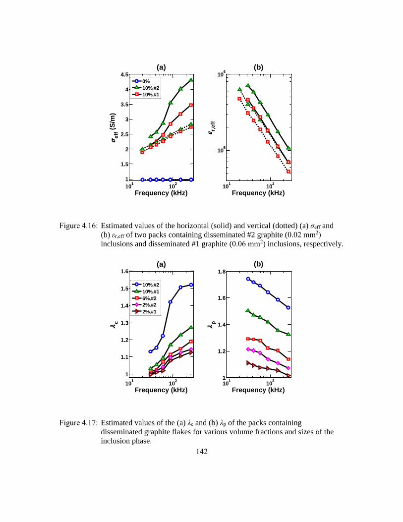
142


(b) εr,eff of two packs containing disseminated #2 graphite (0.02 mm2)

inclusions and disseminated #1 graphite (0.06 mm2) inclusions, respectively.


disseminated graphite flakes for various volume fractions and sizes of the

inclusion phase.

101

102

1

1.5

2

2.5

3

3.5

4

4.5

Frequency (kHz)

e

ff (

S/m

)

(a)

0%

10%,#2

10%,#1

101

102

105

106

Frequency (kHz)

r,

eff

(b)

101

102

1

1.1

1.2

1.3

1.4

1.5

1.6

Frequency (kHz)

c

(a)

10%,#2

10%,#1

6%,#2

2%,#2

2%,#1

101

102

1

1.2

1.4

1.6

1.8

Frequency (kHz)

p

(b)

143

Figure 4.18: Photographs of the 4-inch-diameter, 24-inch-long, glass-bead packs

containing alternating (a) 0-vol% and 6-vol% of dispersed graphite-bearing

layers, (b) 0-vol% and 10-vol% of dispersed graphite-bearing layers, and (c)

0-vol% and 5-vol% of dispersed pyrite-bearing layers fully saturated with

3.75-S/m-conductivity brine.


(b) εr,eff of three packs containing 5-vol% of uniformly distributed #2

graphite inclusions, 10-vol% of uniformly distributed #2 graphite inclusions,

and alternating 0-vol% and 10-vol% of uniformly distributed #2 graphite-

bearing layers, respectively.

101

102

1

1.5

2

2.5

3

3.5

4

4.5

Frequency (kHz)

e

ff (

S/m

)

(a)

0%

5%,#2

10%-0%,#2

10%,#2

101

102

104

105

106

Frequency (kHz)

r,

eff

(b)

a b c

144


(b) εr,eff of two packs containing 10-vol% of uniformly distributed #1

graphite inclusions and alternating 0-vol% and 10-vol% of uniformly

distributed #1 graphite-bearing layers, respectively.


(b) εr,eff of two packs containing 6-vol% of uniformly distributed #1 graphite

inclusions and alternating 0-vol% and 6-vol% of uniformly distributed #1

graphite-bearing layers, respectively.

101

102

1

1.5

2

2.5

3

3.5

Frequency (kHz)

e

ff (

S/m

)

(a)

0%

10%,#1

10%-0%,#1

Avg. (v)

Avg. (h)

101

102

104

105

106

Frequency (kHz)

r,

eff

(b)

101

102

1

1.5

2

2.5

Frequency (kHz)

e

ff (

S/m

)

(a)

0%

6%,#1

6%-0%,#1

Avg. (v)

Avg. (h)

101

102

104

105

106

Frequency (kHz)

r,

eff

(b)

145

Figure 4.22: Estimated values of the (a) λc and (b) λp of two packs containing 5-vol% of

uniformly distributed #1 graphite inclusions and alternating 0-vol% and 10-

vol% of uniformly distributed #2 graphite-bearing layers, respectively.


(b) εr,eff of two packs containing 1.5-vol% of uniformly distributed Pyrite

Red inclusions (red) and #2 graphite inclusions (green), respectively.

101

102

1

1.1

1.2

1.3

1.4

1.5

1.6

Frequency (kHz)

c

(a)

10%-0%,#1

5%,#1

101

102

1.5

2

2.5

3

3.5

4

Frequency (kHz)

p

(b)

101

102

1

1.2

1.4

Frequency (kHz)

e

ff (

S/m

)

(a)

0%

1.5% Gr

1.5% Py

101

102

103

104

105

Frequency (kHz)

r,

eff

(b)

146


(b) εr,eff of three packs containing 2.5-vol% of uniformly distributed Pyrite

Red inclusions (red), 2-vol% of uniformly distributed #1 graphite inclusions

(green), and uniformly distributed mixture of 2-vol% of #1 graphite

inclusions and 2.5-vol% of Pyrite Red inclusions (magenta), respectively.


(b) εr,eff of two packs containing uniformly distributed mixture of 5-vol% of

#2 graphite inclusions and 2.5-vol% of Pyrite Red inclusions (red) and

uniformly distributed mixture of 2-vol% of #1 graphite inclusions and 2.5-

vol% of Pyrite Red inclusions (magenta), respectively.

101

102

0.8

1

1.2

1.4

1.6

1.8

Frequency (kHz)

e

ff (

S/m

)

(a)

0%

2% Gr

2.5% Py

4.5% GrPy

101

102

104

105

Frequency (kHz)

r,

eff

(b)

101

102

0.8

1.2

1.6

2

Frequency (kHz)

e

ff (

S/m

)

(a)

0%

7.5% GrPy

4.5% GrPy

101

102

104

105

Frequency (kHz)

r,

eff

(b)

147

Chapter 5: Mechanistic Model of Interfacial Polarization of

Disseminated Conductive Minerals in Absence of Redox-Active Species

Electrically conductive mineral inclusions are commonly present in organic-rich

mudrock and source-rock formations as veins, laminations, rods, grains, flakes, and beds.

Laboratory and subsurface electromagnetic (EM) measurements performed on

geomaterials containing electrically conductive inclusions generally exhibit frequency

dispersion due to interfacial polarization phenomena at host-inclusion interfaces. In

absence of redox-active species, surfaces of electrically conductive mineral inclusions are

impermeable to the transport of charge carriers, inhibit the exchange of charges, and behave

as perfectly polarized (PP) interfaces under the influence of an externally applied EM field.

Interfacial polarization phenomena involving charge separation, migration,

accumulation/depletion, and relaxation around PP interfaces is referred to as perfectly

polarized interfacial polarization (PPIP); it influences the magnitude and direction of the

electric field and charge carrier migration in the geomaterial. I develop a mechanistic

model to quantify the complex-valued electrical conductivity response of geomaterials

containing electrically conductive mineral inclusions, such as pyrite and magnetite,

uniformly distributed in a fluid-filled, porous matrix made of non-conductive grains

possessing surface conductance, such as silica and clay grains. The model first uses a linear

approximation of Poisson-Nernst-Planck’s (PNP) equations of dilute solution theory to

determine the induced dipole moment of a single isolated conductive inclusion and that of

a single isolated non-conductive grain surrounded by an electrolyte. A consistent effective-

medium formulation is then implemented to determine the effective complex-valued

electrical conductivity of the geomaterial. Our model predictions are in good agreement

with laboratory measurements of multi-frequency complex-valued electrical conductivity,

148

relaxation time, and chargeability of mixtures containing electrically conductive

inclusions.

5.1 INTRODUCTION

Interfacial polarization phenomena influence electromigration, charge carrier

accumulation/depletion, and electrodiffusion processes in host materials (Wong, 1979;

Schmuck and Bazant, 2012). A resistivity interpretation method that neglects interfacial

polarization effects will lead to inaccurate estimation of petrophysical properties of

formations containing electrically conductive inclusions. However, there are limited

publications related to laboratory investigations and numerical modeling of the effects of

interfacial polarization of electrically conductive mineral inclusions on subsurface galvanic

resistivity, EM induction, and EM propagation measurements (Anderson et al., 2006;

Anderson et al., 2008; Wang and Poppitt, 2013). Existing resistivity interpretation

techniques for the three above-mentioned EM measurements do not account for the effects

of interfacial polarization of electrically conductive mineral inclusions (Anderson et al.,

2007; Corley et al., 2010). As a result, conventional resistivity interpretations in pyrite-rich

sedimentary rocks (Altman et al., 2008) and pyrite- and graphite-rich organic source rocks

(Anderson et al., 2008) typically give rise to inaccurate estimates.

In geomaterials, charge carriers in a porous brine-filled host are ions, while those

in an electrically conductive mineral inclusion are holes and electrons (Chu and Bazant,

2006). Redox-active conditions allow charge transfer and charge carrier transport to occur

at host-inclusion interfaces (common surfaces between conductive mineral inclusions and

host). Such redox-active conditions exist only when (a) the pore-filling electrolyte is in

contact with the outer surfaces of electrically conductive inclusions, (b) redox-active

species (for example, Fe3+, O2, and H+ are redox-active species with respect to pyrite) are

149

present in the electrolyte (Placencia-Gomez and Slater, 2014), and (c) the magnitude of the

externally applied EM field is above a certain threshold value (Chu and Bazant, 2006).

Consequently, host-inclusion interfaces in geomaterials containing conductive inclusions

are typically impermeable to charge transport, inhibit charge transfer, and behave as

perfectly polarized interfaces in the presence of weak or moderate externally applied

electric fields.

In this chapter, I focus on the interfacial polarization phenomena occurring in

redox-inactive conditions. I develop and test a new mechanistic electrochemical model,

referred to as the PPIP model, to analyze the EM response of geomaterials containing

uncharged perfectly polarizable spherical, rod-like, and/or sheet-like electrically

conductive inclusions surrounded by either pore-filling conductive/non-conductive fluid or

non-conductive matrix. Notably, the PPIP model is coupled with a surface-conductance-

assisted interfacial polarization (SCAIP) model that accounts for the complex-valued

conductivity response of fluid-filled, porous matrix made of non-conductive spherical

grains possessing surface conductance (Σs). This work is technically significant as

exploration and production activities are shifting toward geologically complex reservoirs

and computationally inexpensive resistivity interpretation methods are required for

purposes of accurate estimation of water saturation, conductivity of formation water, and

organic content.

5.2 INTERFACIAL POLARIZATION PHENOMENA

When the surface of a non-metallic (non-conductive) mineral, such as clay minerals

and silica grains, is exposed to electrolytes, it acquires charges due to ionic adsorption,

protonation/deprotonation of the hydroxyl groups, and dissociation of other potentially

active surface groups (e.g., Leroy and Revil, 2004). In contrast, in redox-inactive

150

conditions, the surface of a metallic or semi-metallic (electrically conductive) mineral, such

as pyrite, graphite, magnetite, and siderite, does not possess surface charge when exposed

to an electrolyte (Chu and Bazant, 2006). However, in presence of an external EM field,

charge carriers (holes and electrons) in electrically conductive mineral inclusions

accumulate at host-inclusion interfaces; consequently, charges are induced on surfaces of

electrically conductive inclusions. It is important to note that the process by which non-

metallic particles acquire surface charges is significantly different from that of metallic and

semi-metallic particles. In this chapter, the mechanism of interfacial polarization and its

effect associated with non-metallic particles is referred to as the SCAIP phenomena, while

that associated with conductive particles is referred to as the PPIP phenomena.

In presence of an externally applied electric field, non-metallic and conductive

particles both develop a counterion cloud and diffused-charge distribution around host-

inclusion interfaces. Variations in the external electric field perturb the charge distribution

around host-inclusion interfaces from its equilibrium state. Therefore, in the presence of a

time-varying electric field, electromigration, charge carrier accumulation/depletion, and

diffusion processes require a certain time, referred to as the relaxation time, to attain the

equilibrium state. Dynamics of accumulation/depletion of charge carriers, relaxation

process, and distribution of charge carrier concentrations around host-inclusion interfaces

influence the magnitude, phase, and frequency dispersion of the EM response of

geomaterials containing electrically conductive inclusions.

5.2.1 Mathematical models of interfacial polarization phenomena

Various mathematical models of accumulation/depletion and relaxation of charge

carriers around surfaces of non-conductive spherical particles possessing surface

conductance have been developed for applications in colloidal (Grosse and Barchini,

151

1992), electrochemical (Chu and Bazant, 2006), microfluidic, biological (Zheng and Wei,

2011), and geophysical (Revil, 2012; Placencia-Gomez and Slater, 2014) measurements.

Modeling of interfacial polarization can be done using circuit (Dias, 2000), empirical

(Tarasov and Titov, 2013), phenomenological (Wait, 1986), or mechanistic models

(Schmuck and Bazant, 2012; Revil et al., 2015a; Revil et al., 2015b). A physically

consistent model must satisfy Kramers-Kronig relations (Olhoeft et al., 1994; Toumelin et

al., 2008).

Schwarz (1962) modeled the interfacial polarization mechanism around charged

particles as a diffusion of counterions moving along the surface of a charged particle. This

modeling framework neglected all the bulk diffusion effects by calculating the potential

outside the counterion layer as a solution of Laplace’s equation rather than Poisson’s

equation. Dukhin et al. (1974) developed a new approach to this problem based on the

concept of a diffused double layer. Non-linearity of the Dukhin et al.’s (1974) equation led

to mathematical complexity which does not provide analytical expressions for the

interfacial polarization process in terms of various relaxation parameters. Subsequently,

Grosse and Foster (1987) developed a simplified model which led to an analytical solution

of interfacial polarization of charged spherical particles in an electrolyte. Previous theories

were improved by Grosse and Barchini (1992) and Wong (1979) for infinitely conductive

spherical particles in an electrolyte with semi-permeable membranes capable of

electrochemical reactions. Different from the above-mentioned models, our model couples

interfacial polarization of uniformly distributed spherical, rod-like, and sheet-like finitely

conductive inclusions in redox-inactive conditions, with the interfacial polarization of the

electrolyte-filled, porous host medium made of spherical, silt- and/or clay-sized grains

possessing surface conductance.

152

5.3 PPIP-SCAIP MODEL

The PPIP model is based on the PNP equations for a dilute solution in a weak

electrical field regime. Using the PNP equations, I analyze the EM response of a

representative volume comprising a single, isolated electrically conductive inclusion

surrounded by the host material (Zheng and Wei, 2011). Subsequently, I employ a

consistent effective-medium formulation to determine the effective complex conductivity

(Keff) of the entire mixture (Grosse and Barchini, 1992). I claim that the PPIP model is

reliable for studying the EM response of mixtures containing uniformly distributed

inclusions of characteristic length < 1 mm, conductivity < 105 S/m, relative permittivity <

20, relative magnetic permeability equal to 1, and volume fraction < 20% in the frequency

range of 100 Hz to 100 MHz. Beyond these limits, the PPIP model predictions will incur

significant discrepancies with measurements due to the skin effect of the inclusion phase.

The skin effect is primarily governed by the operating frequency and conductivity of the

inclusion phase. PPIP model predictions are physically consistent only when the estimated

skin depth is an order of magnitude larger than the characteristic length of the inclusions.

For example, at an operating frequency of 100 kHz, an inclusion phase of conductivity of

103 S/m and εr of 10 exhibits a skin depth of 50 mm. Therefore, the PPIP model can be

used to compute the complex conductivity response of a geological mixture containing

such an inclusion phase at 100 kHz only when the characteristic length of the inclusion

phase is smaller than 5 mm.

The PPIP model is coupled with the SCAIP model for consistent petrophysical

applications. Likewise, the SCAIP model quantifies the complex conductivity response of

fluid-filled, porous host medium, while the PPIP model quantifies the complex

conductivity response of an electrically conductive inclusion phase that is uniformly

153

distributed in the fluid-filled, porous host medium. The integrated PPIP-SCAIP model

assumes negligible EM coupling and dipole-dipole interaction between adjacent

polarizable particles, namely conductive inclusions and non-conductive particles

possessing surface conductance. This chapter develops the mathematical formulation of

the PPIP model for the three geometries, namely sphere, long cylinder, and thin sheet,

while that of the SCAIP model will be documented in a forthcoming publication. For

purposes of model simplification, electrically conductive mineral grains, dispersed clay

mineral grains, and silt- and clay-sized grains of the host medium are identified as isolated

spheres. Further, pore-throat-filling and rod-like mineralization are identified as isolated

parallelly aligned long cylinders; fractures, mineral veins, mineral laminations, and thin

beds are identified as isolated parallelly aligned thin sheets.

Figure 5.1 shows the three types of geological mixtures that can be analyzed using

the PPIP model. Figures 5.2 and 5.3 are schematic depictions of PPIP phenomena in a

representative volume of a dilute mixture of uniformly distributed electrically conductive

spherical, rod-like, or sheet-like inclusions in an electrolyte-saturated host medium. The

representative volume illustrated in Figure 5.2 describes the geological mixtures shown in

Figures 5.1a and 5.1b while that in Figure 5.3 describes the geological mixture shown in

Figure 5.1c. For the representative volume of a mixture containing spherical inclusions

(Figure 5.1a), as shown in Figure 5.2, interfacial polarization is independent of the direction

of the externally applied electric field due to spherical symmetry. On the other hand, for

the representative volume of a mixture containing rod-like inclusions (Figure 5.1b), as

shown in Figure 5.2, interfacial polarization exists only in the transverse radial direction

and is negligible in the axial direction (y-axis). Owing to the azimuthal symmetry of a rod-

like inclusion, interfacial polarization at the cylindrical surface is independent of the

154

azimuth of the incident electric field. By contrast, for the representative volume of a

mixture containing sheet-like inclusions (Figure 5.1c), as shown in Figure 5.3, interfacial

polarization only develops across the XY-plane along the z-axis. In order to exhibit

interfacial polarization, sheet-like inclusions require that the component of the externally

applied electric field along the z-axis be non-zero. Directionality of interfacial polarization

of rod-like and sheet-like inclusions gives rise to electrical anisotropy in formations

containing such inclusions.

The phenomenological basis of interfacial polarization considered in our work

builds on the mechanistic descriptions outlined by Revil et al. (2015a) (see also Placencia-

Gomez and Slater, 2014). Charge carriers in conductive minerals have higher mobility

compared to ions in porous geomaterials. In the presence of an externally applied EM field,

charge carriers in the disseminated electrically conductive inclusions migrate faster and

accumulate at impermeable interfaces. Consequently, electrically conductive inclusions

behave as dipoles in the presence of an externally applied electric field. Subsequently,

charge carriers in the host medium migrate and accumulate on host-inclusion interfaces

under the influence of the externally applied electric field and that of the induced charges

in conductive inclusions. Unlike Wong’s (1979) model, the newly developed PPIP model

integrates the dynamics and distribution of charge carriers inside and outside electrically

conductive inclusions. Therefore, the PPIP model predicts the large dielectric enhancement

and complex conductivity dispersion behavior of mixtures containing conductive

inclusions uniformly distributed in a porous, electrolyte-saturated host.

In the absence of an externally applied electric field, a Guoy-Chapman layer is

assumed around the silt- and clay-sized grains and clay mineral inclusions. A negligible

initial surface charge is also assumed on electrically conductive inclusions. Thus, there is

155

no double layer around the surface of electrically conductive inclusions, whereby the

surface conductance of a conductive inclusion is negligible. Similar assumptions are made

in electrochemistry and colloid science with respect to electrochemical relaxation around

metallic surfaces (Chu and Bazant, 2006). Also, I assume absence of redox-active species

and neglect the influence of pH of pore water (Revil et al., 2015a). The host and inclusion

phases can be modeled as an electrically conductive, insulating, or dielectric material. Also,

pore-filling fluid can be modeled as electrically conductive or non-conductive material.

The host, inclusion, and pore-filling fluid are assumed to have homogeneous, isotropic,

and non-dispersive electrical properties. Therefore, the frequency dispersion and dielectric

enhancement predicted by the PPIP model solely stem from the PPIP phenomenon around

electrically conductive inclusions.

5.3.1 Poisson-Nernst-Planck’s Equations

The PNP equations have been applied to model electromigration and diffusion of

ionic charge carriers in electrolytes (e.g., Zheng and Wei, 2011) and that due to holes and

electrons in semiconductors (e.g., Schmuck and Bazant, 2012). It is based on a mean-field

approximation of charge carrier interactions and continuum descriptions of concentration

and electrostatic potential. I apply the PNP equations to model charge dynamics and

relaxation in the representative volume (Figures 5.2 and 5.3) containing only two phases,

namely the host medium, denoted by subscript h, and the electrically conductive inclusion

phase, denoted by subscript i. The host medium can be either an electrolyte or the non-

conductive matrix. At time t < 0, it is assumed that there is no external electric field exciting

the representative volume. Also, spontaneous initial accumulation of charges is assumed

to be absent on the host-interfaces. At time t < 0, electro-neutrality is assumed throughout

the system. Initial charge carrier densities at equilibrium conditions in both the host and

156

inclusion phases are denoted as 𝑁0,𝑗, where subscript j takes the form of i for the inclusion

phase and h for the host phase. At time t = 0, the representative volume experiences an

uniform externally applied electric field 𝐸 = 𝐸0ei𝜔𝑡, where 𝐸0 is the amplitude of the

externally applied electric field, i is square root of -1, and 𝜔 is the frequency of the

externally applied electric field. Under a weak field approximation, charge carrier densities

in host and inclusion phases are perturbed from their equilibrium conditions near the host-

inclusion interfaces, resulting in a new linearly approximated charge distribution given by

𝑁𝑗±(𝑟) = 𝑁0,𝑗 + 𝑐𝑗

±(𝑟)ei𝜔𝑡 cos(𝜃) , (1)

such that |𝑐𝑗±| ≤ 𝑁0,𝑗

± , 𝑐𝑗± is the charge density variation due to the externally applied

electric field near the host-inclusion interface in medium j, 𝑟 is the distance along the

normal to the interface, and 𝜃 is the angle between the normal to the interface and the

incident external electric field. Further, the symbol “+” identifies positive-charge carriers

such as holes and cations, while the symbol “-” identifies negative-charge carriers such as

electrons and anions.

I use a low-frequency approximation that requires that 𝜔 be much smaller

than 𝑎2 𝜆𝐷2⁄ , where 𝜆D is the Debye screening length and a is the characteristic length of

the inclusion phase. The characteristic length 𝑎 is equal to the radius of spherical inclusion,

radius of rod-like inclusion, or half of the thickness of sheet-like inclusion. Mathematically,

𝜆D = √휀ℎkB𝑇 (2𝑍ℎ+𝑍ℎ

−q2𝑁0,ℎ)⁄ , where 휀ℎ is dielectric permittivity of the host, kB is

Boltzmann’s constant, 𝑇 is absolute temperature, 𝑍ℎ± is charge number of positive and

negative charge carriers in the host, and q is the elementary charge. One of our simplifying

assumptions is that all the charge carriers bear unitary charge and that both host and

inclusion phases bear binary, symmetric charge carriers. In other words,

𝑍𝑗± = 1, 𝜇ℎ

+ = 𝜇ℎ− = 𝜇ℎ, 𝜇𝑖

+ = 𝜇𝑖− = 𝜇𝑖, 𝑁0,𝑖

+ = 𝑁0,𝑖− = 𝑁0,𝑖 ; 𝑁0,ℎ

+ = 𝑁0,ℎ− = 𝑁0,ℎ, (2)

157

where 𝜇𝑗± is the electrical mobility of positive and negative charge carriers in medium j,

and 𝑍𝑗± is charge number of positive and negative charge carriers in medium j.

The current density of each charge carrier type in the host and inclusion phases is

the sum of current density due to drift current and diffusion current. In the absence of

generation/recombination reactions, the transport equation representing conservation laws

for charge-carrying species can be written as

𝐣𝑗± = 𝐣𝑗,drift

± + 𝐣𝑗,diffusion± = q𝑁𝑗

±𝜇𝑗𝐞𝑗 ∓ q𝐷𝑗±∇𝑁𝑗

±, (3)

where 𝐣𝑗± is the current density of positive and negative charge carriers, respectively, in

medium j, 𝐞𝑗 is the net electric field vector in medium j, and 𝐷𝑗± is diffusion coefficient of

positive and negative charge carriers, respectively, in medium j. When using the

simplifying assumption for electrical mobility of charge carriers, as mentioned in equation

2, and Einstein’s relationship of diffusion coefficient with electrical mobility, namely 𝐷𝑗 =

(𝜇𝑗kB𝑇) q⁄ , I obtain

𝐷ℎ+ = 𝐷ℎ

− = 𝐷ℎ, 𝐷𝑖+ = 𝐷𝑖

− = 𝐷𝑖. (4)

By substituting 𝐞𝑗 = −∇𝜑𝑗 into the low-frequency limit of Maxwell’s equations

(induction neglected) and substituting equation 4 into equation 3, I express the charge

species conservation condition as

𝐣𝑗± = −q𝑁𝑗

±𝜇𝑗∇𝜑𝑗 ∓ q𝐷𝑗∇𝑁𝑗±, (5)

where 𝜑𝑗 is the electrical potential in medium j. Equation 5 is Nernst-Planck’s equation

that describes the relationship of the flux of charge-carrying species to its concentration

gradient and that to the applied electrical potential gradient in a given medium. Nernst-

Planck’s equation can alternatively be expressed as

𝐣𝑗± = −𝐷𝑗

±𝑁𝑗±∇𝜑𝑐𝑗

± , (6)

where 𝜑𝑐𝑗± = kB𝑇ln(𝑁𝑗

±) ± q𝑍𝑗±𝜑𝑗 is the electrochemical potential of charge carriers.

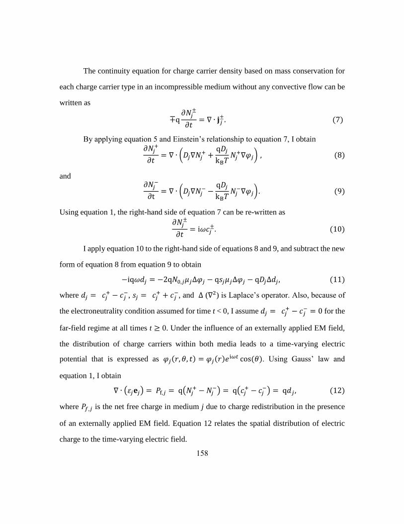
158

The continuity equation for charge carrier density based on mass conservation for

each charge carrier type in an incompressible medium without any convective flow can be

written as

∓q𝜕𝑁𝑗

±

𝜕𝑡= ∇ ∙ 𝐣𝑗

±. (7)

By applying equation 5 and Einstein’s relationship to equation 7, I obtain

𝜕𝑁𝑗+

𝜕𝑡= ∇ ∙ (𝐷𝑗∇𝑁𝑗

+ +q𝐷𝑗

kB𝑇𝑁𝑗

+∇𝜑𝑗) , (8)

and ∂𝑁𝑗

−

∂t= ∇ ∙ (𝐷𝑗∇𝑁𝑗

− −q𝐷𝑗

kB𝑇𝑁𝑗

−∇𝜑𝑗). (9)

Using equation 1, the right-hand side of equation 7 can be re-written as

𝜕𝑁𝑗±

𝜕𝑡= i𝜔𝑐𝑗

±. (10)

I apply equation 10 to the right-hand side of equations 8 and 9, and subtract the new

form of equation 8 from equation 9 to obtain

−iq𝜔𝑑𝑗 = −2q𝑁0,𝑗𝜇𝑗∆𝜑𝑗 − q𝑠𝑗𝜇𝑗∆𝜑𝑗 − q𝐷𝑗∆𝑑𝑗 , (11)

where 𝑑𝑗 = 𝑐𝑗+ − 𝑐𝑗

−, 𝑠𝑗 = 𝑐𝑗+ + 𝑐𝑗

−, and ∆ (∇2) is Laplace’s operator. Also, because of

the electroneutrality condition assumed for time t < 0, I assume 𝑑𝑗 = 𝑐𝑗+ − 𝑐𝑗

− = 0 for the

far-field regime at all times t ≥ 0. Under the influence of an externally applied EM field,

the distribution of charge carriers within both media leads to a time-varying electric

potential that is expressed as 𝜑𝑗(𝑟, 𝜃, 𝑡) = 𝜑𝑗(𝑟)𝑒i𝜔𝑡 cos(𝜃). Using Gauss’ law and

equation 1, I obtain

∇ ∙ (휀𝑗𝐞𝑗) = 𝑃f,𝑗 = q(𝑁𝑗+ − 𝑁𝑗

−) = q(𝑐𝑗+ − 𝑐𝑗

−) = q𝑑𝑗 , (12)

where 𝑃𝑓,𝑗 is the net free charge in medium j due to charge redistribution in the presence

of an externally applied EM field. Equation 12 relates the spatial distribution of electric

charge to the time-varying electric field.

159

Assuming that both media are linear, isotropic, and homogeneous, and that the

electric field can be defined by a scalar electrical potential field, 𝜑𝑗, I obtain

∇ ∙ (휀𝑗𝐞𝑗) = −∇ ∙ (휀𝑗∇𝜑𝑗) = −휀𝑗∆𝜑𝑗. (13)

By combining equations 12 and 13, I obtain an alternate expression of Poisson’s

equation, given by

∆𝜑𝑗 = −q𝑑𝑗

휀𝑗. (14)

Poisson’s equation is applied to describe the electric field in terms of the electrical

potential, the gradient of which governs electromigration in both media. Under the weak

field approximation, by substituting equation 14 into equation 11, I obtain the PNP

equations, given by

−iq𝜔𝑑𝑗 =2q2𝑁0,𝑗𝜇𝑗𝑑𝑗

휀𝑗⁄ − q𝐷𝑗∆𝑑𝑗 , (15)

which can be re-written as

∆𝑑𝑗 = (i𝜔

𝐷𝑗+

𝜎𝑗

휀𝑗𝐷𝑗) 𝑑𝑗 , (16)

where 𝜎𝑗=2𝑁0𝑗𝜇𝑗q is the electrical conductivity of medium j, 휀𝑗 = 휀r,𝑗휀0 is the dielectric

permittivity of medium j, 휀𝑟,𝑗 is the relative permittivity of medium j, and 휀0 = 8.854 ×

10−12 F m⁄ is vacuum permittivity. I rewrite equation 16 as

∆𝑑𝑗 = 𝛾𝑗2𝑑𝑗, (17)

where

𝛾𝑗2 = (

i𝜔

𝐷𝑗+

𝜎𝑗

휀𝑗𝐷𝑗). (18)

Equation 17 is a Helmholtz partial differential equation that can be solved by

separation of variables in Cartesian, cylindrical, or spherical coordinates to obtain an

analytical expression for 𝑑𝑗 in the host and inclusion phases around the perfectly polarized

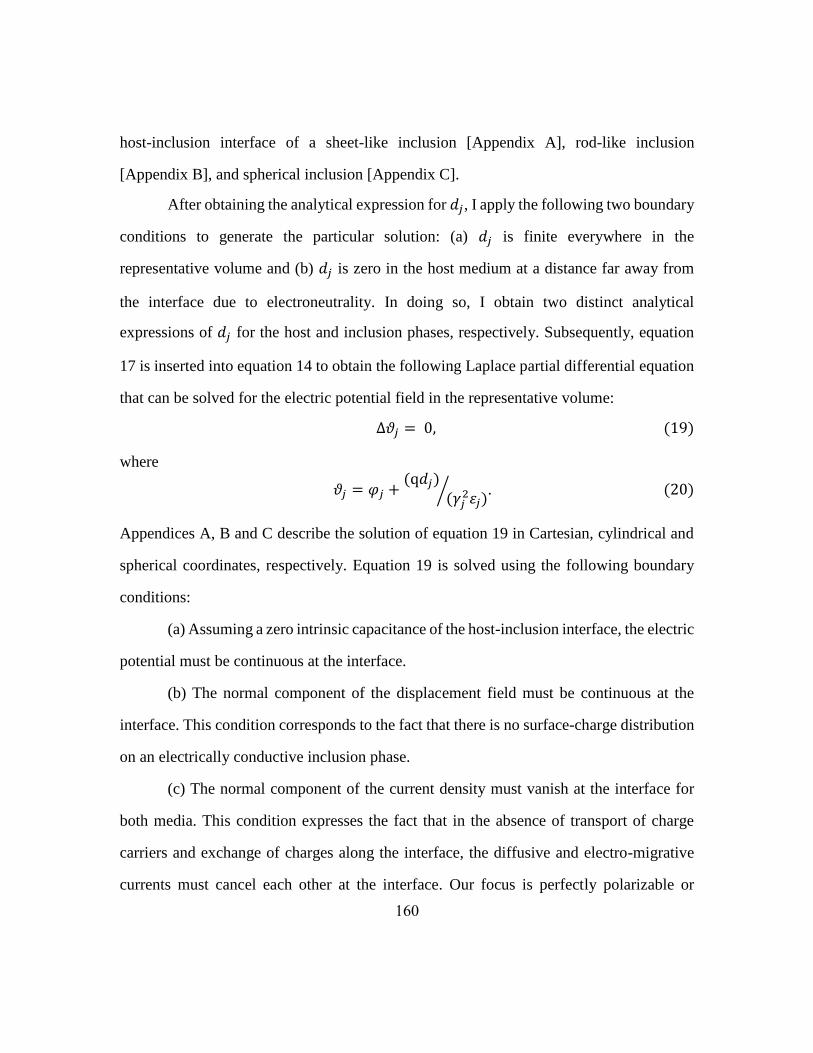
160

host-inclusion interface of a sheet-like inclusion [Appendix A], rod-like inclusion

[Appendix B], and spherical inclusion [Appendix C].

After obtaining the analytical expression for 𝑑𝑗, I apply the following two boundary

conditions to generate the particular solution: (a) 𝑑𝑗 is finite everywhere in the

representative volume and (b) 𝑑𝑗 is zero in the host medium at a distance far away from

the interface due to electroneutrality. In doing so, I obtain two distinct analytical

expressions of 𝑑𝑗 for the host and inclusion phases, respectively. Subsequently, equation

17 is inserted into equation 14 to obtain the following Laplace partial differential equation

that can be solved for the electric potential field in the representative volume:

∆𝜗𝑗 = 0, (19)

where

𝜗𝑗 = 𝜑𝑗 +(q𝑑𝑗)

(𝛾𝑗2휀𝑗)⁄ . (20)

Appendices A, B and C describe the solution of equation 19 in Cartesian, cylindrical and

spherical coordinates, respectively. Equation 19 is solved using the following boundary

conditions:

(a) Assuming a zero intrinsic capacitance of the host-inclusion interface, the electric

potential must be continuous at the interface.

(b) The normal component of the displacement field must be continuous at the

interface. This condition corresponds to the fact that there is no surface-charge distribution

on an electrically conductive inclusion phase.

(c) The normal component of the current density must vanish at the interface for

both media. This condition expresses the fact that in the absence of transport of charge

carriers and exchange of charges along the interface, the diffusive and electro-migrative

currents must cancel each other at the interface. Our focus is perfectly polarizable or

161

completely blocking interfaces without Faradic processes, wherein fluxes of charge carriers

must vanish on both sides of the interface.

A limitation of the PNP equations arises from the omission of the finite volume

effect of charge carriers, mutual interactions and steric effects, effects due to transport of

ions in confined channels of the pore system, and correlation effects (Chu and Bazant,

2006). Another limitation arises because the model is developed only for symmetric, binary

charge carriers in both the host and inclusion phases. This assumption simplifies the

analytical complexity of the PNP formulations. Another drawback of the PNP formulations

is that the analysis is performed for materials that contain completely dissociated charge

carriers at low concentration values. Moreover, in this chapter, unlike Chu and Bazant

(2006), I only consider the linear response to weak fields where exact solutions are

possible.

5.3.2 Effective medium model

In geophysical applications, it is desirable to treat a mesoscopically heterogeneous

mixture as a macroscopically homogeneous medium. Such homogenization is done by

constructing the final macroscale material incrementally from a starting microscopic

material. First, microscopic electrical properties around a single inclusion/scatter are

computed using the PNP equations, as explained in the previous section. Dipolarizability

(dipole moment), 𝑓(𝜔), of the representative volume, as shown in Appendices A, B, and

C for different geometries of the inclusion, are computed using the PNP equations. In our

derivations of the PNP equations, the effect of multipoles are neglected as their magnitude

decreases with inverse power of distance (Sihvola, 2007). Also, I neglect monopole effects

because there is zero net charge due to the assumed electroneutrality of the mixture. After

calculating the dipolarizability of the representative volume, the global macroscopic

162

electrical properties are computed using effective-medium formulations which are based

on the concept that a material composed of a mixture of distinct homogeneous media can

be considered as a homogeneous material at a sufficiently large observation scale

(Giordano, 2003). Modeling of effective electrical properties of heterogeneous materials

requires information about (a) the number of phases constituting the mixture; (b)

geometrical shapes and sizes of individual phases; and (c) the electrical properties of

individual phases, their distribution, and their interfacial properties.

In this chapter, I primarily focus on estimating effective electrical properties of

mixtures having less than 20% volume fraction of electrically conductive inclusions, which

lies within the limits of Maxwell-Garnett effective-medium formulations. Moreover, for

purposes of petrophysical studies, reservoir rocks have less than 10% volume fraction of

conductive mineral inclusions. Therefore, I implement a Maxwell-Garnett-type effective-

medium formulation to obtain the effective electrical properties. Such a formulation

neglects EM interactions between heterogeneities. Due to the assumed dilution of the

uniformly distributed inclusion phase, individual elements of the dispersed phase are

assumed to be isolated and not in contact with each other. Similar to other mixing theories,

our model includes the assumption that the magnitude of spatial variations of the electric

field is smaller than the magnitude of variations in the intrinsic electrical properties and

geometrical structures. Moreover, all calculations are performed using a quasi-static

assumption that requires the size of heterogeneities to be much smaller than the wavelength

of the applied EM field (Cosenza et al., 2009). Also, when dealing with a lossy medium,

the skin depth of the EM wave must be considered to avoid strong attenuation of the field

amplitudes in the heterogeneities. Most importantly, due to the implementation of the PNP

163

equations, and unlike other theories (e.g., Giordano, 2003), our effective-medium

formulations explicitly account for the characteristic lengths of heterogeneities.

For a monodispersed mixture of ellipsoidal inclusions, the effective-medium model

of the mixture can be written in terms of the complex-valued conductivity (Giordano, 2003)

as 𝐾�̂�,eff − 𝐾ℎ

𝐾�̂�,eff + 𝑛�̂�𝐾ℎ=

𝑖

𝐾𝑖 − 𝐾ℎ

𝐾𝑖 + 𝑛�̂�𝐾ℎ, (21)

which can also be expressed as 𝐾�̂�,eff − 𝐾ℎ

𝐾�̂�,eff + 𝑛�̂�𝐾ℎ=

𝑖𝑓�̂�(𝜔), (22)

where 𝐾 = 𝜎 + i𝜔휀 is a representation of the complex conductivity of a material, 𝐾�̂�,eff is

the effective complex conductivity of the geological mixture along the �̂� unit vector that

can be measured with respect to the component of the externally applied electric field

directed along the �̂� unit vector, 𝐾ℎ is the complex-valued conductivity of the homogenous

isotropic host material that surrounds the inclusions, 𝐾𝑖 is the complex-valued conductivity

of the homogenous isotropic inclusion material, 𝑖 is the volume fraction of the inclusion

phase in the mixture, 𝑛�̂� is the shape factor of the inclusion phase along the �̂� unit vector,

and 𝑓�̂�(𝜔) is the dipolarizability of the representative volume along the direction of �̂� unit

vector. Dipolarizability of the representative volume is derived in Appendices A, B, and C

using the PNP equations. In the absence of interfacial polarization, equation 21 is used for

purposes of Maxwell-Garnett’s effective-medium formulation (Sihvola, 2007). However,

for our study, where I model large induced dielectric polarization phenomena, equation 21

will lead to erroneous results because 𝐾𝑖 is drastically altered due to interfacial polarization

around the electrically conductive inclusions. Therefore, equation 22 should be used for

164

effective-medium formulations of the PPIP model (Wong, 1979; Grosse and Barchini,

1992). Additionally, in equations 21 and 22, the shape factor can be expressed as

𝑛�̂� = 1 − 𝐿�̂�

𝐿�̂�, (23)

where 𝐿�̂� is the depolarization factor of the inclusion phase in the direction of the �̂� unit

vector (Sihvola, 2007).

As derived in Appendix A, for a sheet-like inclusion (Figure 5.3) that comprises

the representative volume of a formation containing uniformly distributed, parallelly

aligned, thin beds, laminations, veins, or induced fractures (Figure 5.1c), the

dipolarizability can be expressed as

𝑓(𝜔) = (1 −𝐾ℎ

𝐾𝑖) +

i

𝜔𝑎[𝐾ℎ

𝐾𝑖

𝜎𝑖

휀𝑖

𝐹𝑖

𝐻𝑖−

𝜎ℎ

휀ℎ

𝐸ℎ

𝐺ℎ]. (24)

Additionally, the directional Keff response for a mixture containing sheet-like inclusions

can be computed by substituting equation 24 into equation 22, and next by implementing

the following expressions for the depolarization factor, as mentioned in Giordano (2003):

𝐿�̂� = 𝐿�̂� = 0; 𝐿�̂� = 1,

and

𝑛�̂� = 𝑛�̂� = ∞; 𝑛�̂� = 0.

As a result, the Keff of such a mixture (Figure 5.1c) is significantly altered along the z-axis

and negligibly altered along the x- and y-axes.

Similarly, as derived in Appendix B, for a rod-like inclusion (Figure 5.2) that

comprises the representative volume of a formation containing uniformly distributed pore-

throat-filling or rod-like mineralization (Figure 5.1b), the dipolarizability can be expressed

as

𝑓(𝜔) = −1 +2i𝜔

[1𝑎

𝐾ℎ

𝐾𝑖

𝜎𝑖

휀𝑖

𝐹𝑖

𝐻𝑖−

1𝑎

𝜎ℎ

휀ℎ

𝐸ℎ

𝐺ℎ+ i𝜔(

𝐾ℎ

𝐾𝑖+ 1)]

. (25)

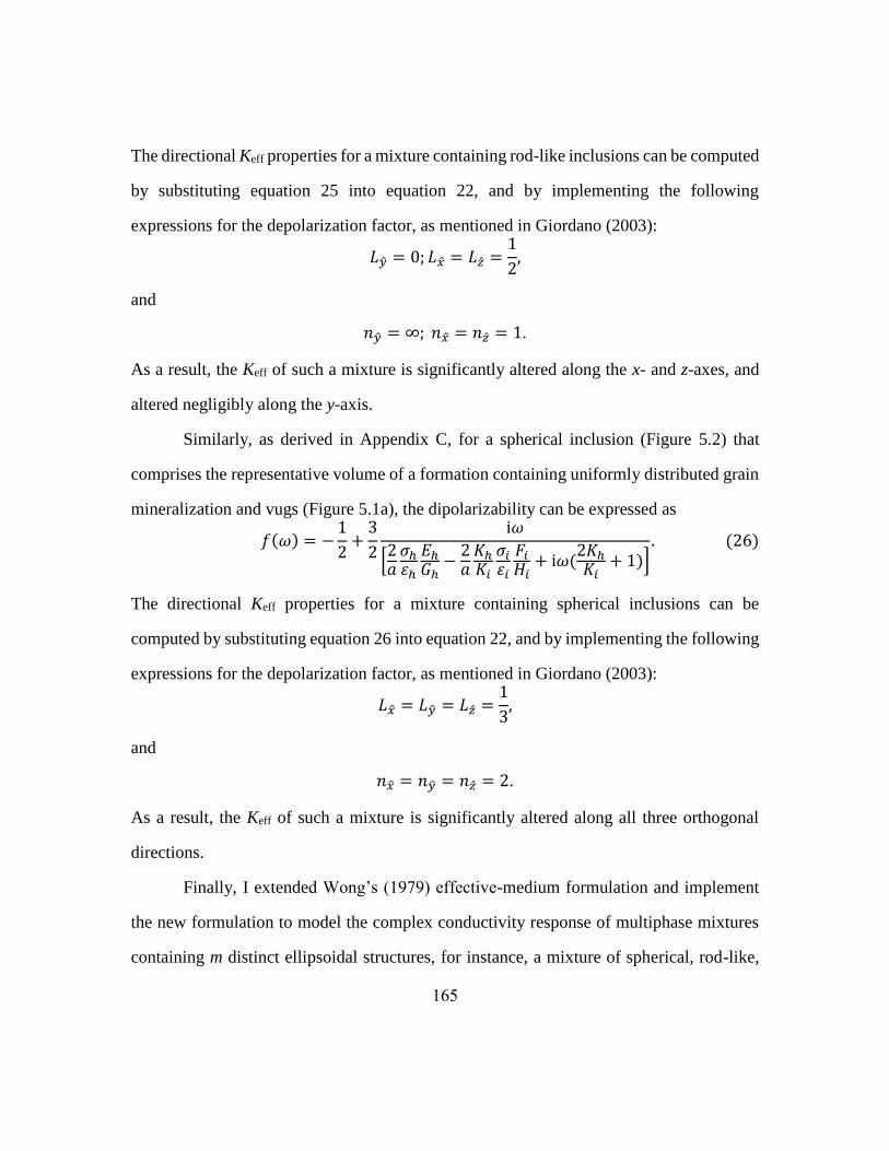
165

The directional Keff properties for a mixture containing rod-like inclusions can be computed

by substituting equation 25 into equation 22, and by implementing the following

expressions for the depolarization factor, as mentioned in Giordano (2003):

𝐿�̂� = 0; 𝐿�̂� = 𝐿�̂� =1

2,

and

𝑛�̂� = ∞; 𝑛�̂� = 𝑛�̂� = 1.

As a result, the Keff of such a mixture is significantly altered along the x- and z-axes, and

altered negligibly along the y-axis.

Similarly, as derived in Appendix C, for a spherical inclusion (Figure 5.2) that

comprises the representative volume of a formation containing uniformly distributed grain

mineralization and vugs (Figure 5.1a), the dipolarizability can be expressed as

𝑓(𝜔) = −1

2+

3

2

i𝜔

[2𝑎

𝜎ℎ

휀ℎ

𝐸ℎ

𝐺ℎ−

2𝑎

𝐾ℎ

𝐾𝑖

𝜎𝑖

휀𝑖

𝐹𝑖

𝐻𝑖+ i𝜔(

2𝐾ℎ

𝐾𝑖+ 1)]

. (26)

The directional Keff properties for a mixture containing spherical inclusions can be

computed by substituting equation 26 into equation 22, and by implementing the following

expressions for the depolarization factor, as mentioned in Giordano (2003):

𝐿�̂� = 𝐿�̂� = 𝐿�̂� =1

3,

and

𝑛�̂� = 𝑛�̂� = 𝑛�̂� = 2.

As a result, the Keff of such a mixture is significantly altered along all three orthogonal

directions.

Finally, I extended Wong’s (1979) effective-medium formulation and implement

the new formulation to model the complex conductivity response of multiphase mixtures

containing m distinct ellipsoidal structures, for instance, a mixture of spherical, rod-like,

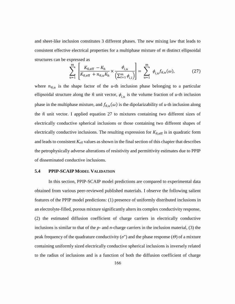
166

and sheet-like inclusion constitutes 3 different phases. The new mixing law that leads to

consistent effective electrical properties for a multiphase mixture of m distinct ellipsoidal

structures can be expressed as

∑

m

u=1

[𝐾�̂�,eff − 𝐾h

𝐾�̂�,eff + 𝑛�̂�,𝑢𝐾h×

𝑖,𝑢

(∑ 𝑖,𝑙

𝑚𝑙=1 )

] = ∑

m

u=1

𝑖,𝑢

𝑓�̂�,𝑢(𝜔), (27)

where 𝑛�̂�,𝑢 is the shape factor of the u-th inclusion phase belonging to a particular

ellipsoidal structure along the �̂� unit vector, 𝑖,𝑢

is the volume fraction of u-th inclusion

phase in the multiphase mixture, and 𝑓�̂�,𝑢(𝜔) is the dipolarizability of u-th inclusion along

the �̂� unit vector. I applied equation 27 to mixtures containing two different sizes of

electrically conductive spherical inclusions or those containing two different shapes of

electrically conductive inclusions. The resulting expression for 𝐾�̂�,eff is in quadratic form

and leads to consistent Keff values as shown in the final section of this chapter that describes

the petrophysically adverse alterations of resistivity and permittivity estimates due to PPIP

of disseminated conductive inclusions.

5.4 PPIP-SCAIP MODEL VALIDATION

In this section, PPIP-SCAIP model predictions are compared to experimental data

obtained from various peer-reviewed published materials. I observe the following salient

features of the PPIP model predictions: (1) presence of uniformly distributed inclusions in

an electrolyte-filled, porous mixture significantly alters its complex conductivity response,

(2) the estimated diffusion coefficient of charge carriers in electrically conductive

inclusions is similar to that of the p- and n-charge carriers in the inclusion material, (3) the

peak frequency of the quadrature conductivity (σ") and the phase response (Θ) of a mixture

containing uniformly sized electrically conductive spherical inclusions is inversely related

to the radius of inclusions and is a function of both the diffusion coefficient of charge

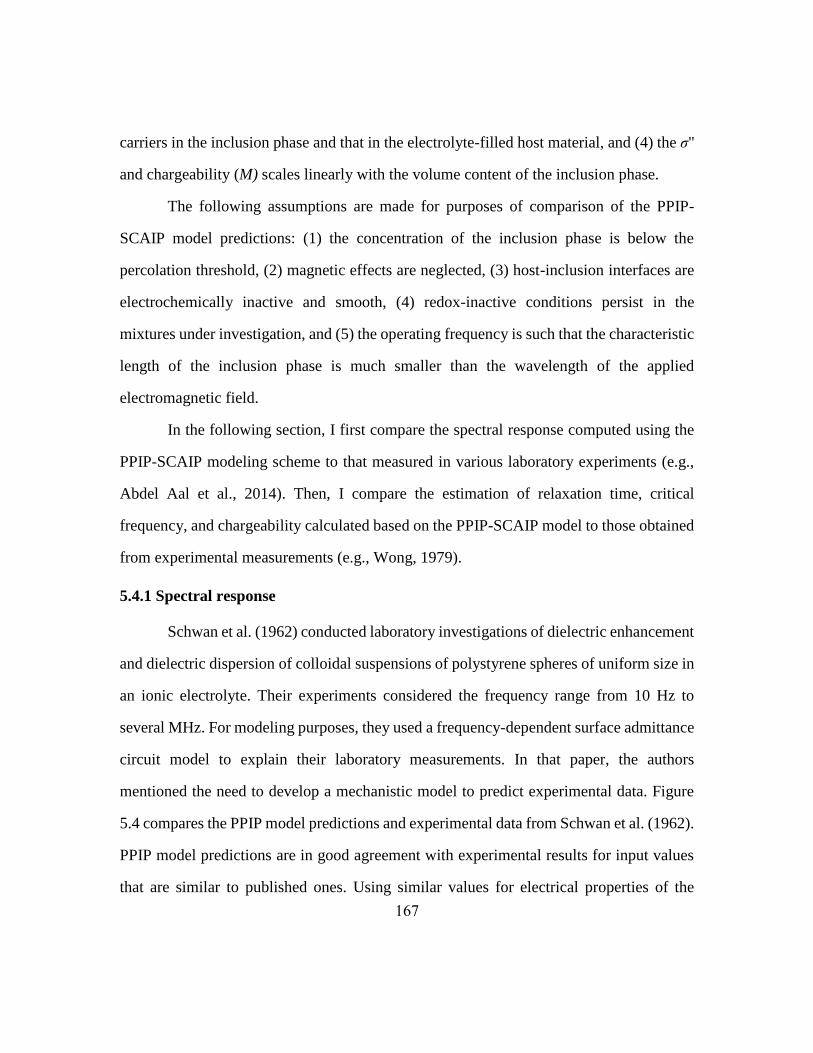
167

carriers in the inclusion phase and that in the electrolyte-filled host material, and (4) the σ"

and chargeability (M) scales linearly with the volume content of the inclusion phase.

The following assumptions are made for purposes of comparison of the PPIP-

SCAIP model predictions: (1) the concentration of the inclusion phase is below the

percolation threshold, (2) magnetic effects are neglected, (3) host-inclusion interfaces are

electrochemically inactive and smooth, (4) redox-inactive conditions persist in the

mixtures under investigation, and (5) the operating frequency is such that the characteristic

length of the inclusion phase is much smaller than the wavelength of the applied

electromagnetic field.

In the following section, I first compare the spectral response computed using the

PPIP-SCAIP modeling scheme to that measured in various laboratory experiments (e.g.,

Abdel Aal et al., 2014). Then, I compare the estimation of relaxation time, critical

frequency, and chargeability calculated based on the PPIP-SCAIP model to those obtained

from experimental measurements (e.g., Wong, 1979).

5.4.1 Spectral response

Schwan et al. (1962) conducted laboratory investigations of dielectric enhancement

and dielectric dispersion of colloidal suspensions of polystyrene spheres of uniform size in

an ionic electrolyte. Their experiments considered the frequency range from 10 Hz to

several MHz. For modeling purposes, they used a frequency-dependent surface admittance

circuit model to explain their laboratory measurements. In that paper, the authors

mentioned the need to develop a mechanistic model to predict experimental data. Figure

5.4 compares the PPIP model predictions and experimental data from Schwan et al. (1962).

PPIP model predictions are in good agreement with experimental results for input values

that are similar to published ones. Using similar values for electrical properties of the

168

polystyrene particles and electrolyte, I obtain good agreement for the computed εr of the

suspension with another set of experimental results mentioned in Schwan et al. (1962), as

shown in Figure 5.5. Figures 5.4 and 5.5 imply that the presence of dispersed polystyrene

particles produces drastic dielectric enhancement and dispersion due to interfacial

polarization phenomena because neither the host nor the inclusion individually possess

dielectric characteristics comparable to that measured in the experiments. On the other

hand, Figures 5.4 and 5.5 indicate relatively smaller conductivity dispersion in the order of

1% relative difference between the high- and low-frequency values of conductivity, which

is attributed to the absence of high-mobility charge carriers in the inclusion phase. Further,

Figure 5.5 shows that PPIP modeling results match EM measurements of oil-in-water

emulsions performed by Hanai et al. (1959).

Hanai et al. (1979) measured the EM response of suspensions of bovine

erythrocytes in a NaCl solution. These biological suspensions of erythrocyte cells exhibit

dielectric relaxation due to interfacial polarization at insulating host-inclusion interfaces

formed of thin-lipidic cell membranes. The representative volume of this mixture is formed

of conducting cytoplasm surrounded by a non-conducting shell of lipidic membrane

immersed in an ionic electrolyte. PPIP modeling of the EM response of such biological

suspensions (Hanai et al., 1979) showed good agreement between the PPIP modeling

results and measured values, as shown in Figure 5.6. In this experiment, cell walls act as

perfectly polarized interfaces. Further, I modeled experiments performed by Delgado et al.

(1998), who worked on identifying laboratory techniques to differentiate surface from

volume diffusion mechanisms. They carried out dielectric dispersion measurements on

suspensions of polymer latex balls in a KCl solution. PPIP modeling results matched

169

experimental results for two different volume fractions of polymer latex balls in a KCl

solution, as shown in Figure 5.7.

Mahan et al. (1986) measured the complex resistivity responses of synthetic

samples containing quartz grains of various sizes and conductive sulphide particles of

different materials that were fully saturated with electrolytes with or without active ions

(e.g., Cu2+ ions are active ions with respect to chalcopyrite mineral inclusions). Active ions

results in charge transfer across host-inclusion interfaces due to oxidation-reduction

reactions. Mahan et al. (1986) were successful in matching laboratory measurements of the

complex resistivity of synthetic samples using Wong’s (1979) model in the frequency

range where frequency dispersion and peak of Θ occur. A limitations of Wong’s (1979)

model is the assumption that inclusions have infinite conductivity and the host behaves as

a non-polarizable ionic material rather than as a mixture of electrolyte and silica grains that

exhibit interfacial polarization arising from electrochemical effects of surface conductance

(also, referred to as the SCAIP phenomenon). The PPIP-SCAIP model does not suffer from

the limitations of Wong’s (1979) model. Unlike Mahan et al.’s (1986) modeling procedure,

the PPIP-SCAIP model takes into account the effects of surface conductance of uniformly

distributed 80-μm diameter spherical silica grains that are fully saturated with pore-filling

fluid. As shown in Figure 5.8a, the PPIP-SCAIP model predictions match very well the

computed results from Mahan et al. (1986) for the complex conductivity response of a

mixture of chalcopyrite and silica grains fully saturated with a NaCl solution that contains

no active ions. The PPIP-SCAIP model predicts a Debye-type dispersion response in the

absence of active ions. On the other hand, for the mixture of quartz and pyrite grains fully

saturated with a NaCl solution that contains active ions, electrochemical charge transfer

reactions occur at interfaces giving rise to a Warburg-type response, as shown in Figure

170

5.8b. As a result, the agreement between PPIP-SCAIP model predictions and experimental

results worsens at higher frequencies for this mixture. Electrochemical charge transfer

reaction at the interface due to active ions alters the boundary conditions at the interface

assumed in our present study.

Importantly, the PPIP-SCAIP model was implemented to estimate the diffusion

coefficient of charge carriers in the inclusion phase and the resistivity of inclusions. These

estimated values are in good agreement with the physical properties of the inclusion

materials, as mentioned in Revil et al. (2015a). The estimated resistivity of pyrite is 5 times

higher than that of chalcopyrite, while the diffusion coefficient of charge carriers in pyrite

is an order of magnitude larger than that of chalcopyrite. Due to the dynamics of charge

carriers in the electrically conductive inclusion, I observe 13% relative difference between

low- and high-frequency resistivity values, which is significantly larger than that obtained

for mixtures containing non-conductive inclusions (e.g., Schwan et al., 1962).

Abdel Aal et al. (2014) performed laboratory experiments to investigate the

complex conductivity signatures of five minerals, namely pyrite, magnetite, goethite,

hematite, and siderite, disseminated in porous media under variable iron mineral content

and grain size. PPIP-SCAIP model predictions are in good agreement with laboratory

measurements. The PPIP-SCAIP model was implemented to estimate the diffusion

coefficient of charge carriers in pyrite inclusions to be 1×10-6 m2s-1, which is comparable

to the diffusion coefficient of charge carriers in metallic grains equal to 2.5×10-5 m2s-1 for

p-charge carriers and 3×10-6 m2s-1 for n-charge carriers as estimated from laboratory

measurements carried out by Revil et al. (2015a). Figure 5.9 shows that PPIP-SCAIP

modeling results agree with experimental values for uniformly distributed pyrite mineral

inclusions in sand matrix fully saturated with a NaCl solution. I observe an increase in the

171

magnitude of the peak of σ" and a progressive shift in relaxation peak toward higher

frequencies with a decrease in the diameter of pyrite inclusions. Also, I observe that the

increase in in-phase conductivity (σ') is much smaller than that of the σ" because of the low

values of conductivity of the pore-filling electrolyte.

Tirado and Grosse (2006) performed broadband dielectric measurements on

suspensions of spherical polystyrene particles having high surface charge distribution in an

aqueous solution. Instead of using the PPIP-SCAIP model, I used only the SCAIP model

to quantify the dielectric enhancement and dispersion behavior of suspensions measured

by Tirado and Grosse (2006). Interfacial polarization phenomena in their experiment is

dominated by surface conductance effects due to high surface charge of polystyrene

particles. Figure 5.11 shows a good agreement between Tirado and Grosse’s (2006)

measurements and SCAIP model predictions. This agreement validates the use of the

SCAIP model in quantifying the interfacial polarization arising from surface conductance

effects of quartz and clay grains.

5.4.2 Relaxation time and critical frequency

PPIP model predictions generate a complex conductivity response having Debye-

like characteristics that is consistent with various laboratory measurements on mixtures

containing conductive inclusions (e.g., Wong, 1979). As shown in Figure 5.13a, the PPIP

model predicts a linear relationship between relaxation time (𝜏) and radius of electrically

conductive spherical inclusions. This linear relationship can also be expressed as an inverse

relationship of critical frequency and radius of conductive spherical inclusions, as

illustrated in Figure 5.12, which compares PPIP model predictions against Wong’s (1979)

modeling results. Specifically, Figure 5.12 implies that an inverse relationship exists only

when active ions are not present in the electrolyte and when the radius of uniformly

172

distributed conductive spherical inclusions are lower than 50 µm. Further, PPIP model

predictions of the linear relationship of 𝜏 with radius of conductive spherical inclusions is

in accordance with the theoretical derivation by Shilov and Borkovskaya (2010), where

they show that the critical frequency of -dispersion (Maxwell-Wagner-type relaxations)

is inversely related to the radius of conductive spherical inclusions for medium and high

frequencies. On the other hand, at low frequencies, Shilov and Borkovskaya (2010) show

that the critical frequency of -dispersion (concentration polarization due to surface

conductance) for a mixture containing only non-conductive inclusions possessing surface

conductance is related to the radius of inclusions by an inverse square law, also determined

by Dukhin et al. (1974). Furthermore, unlike previously published research work

describing PPIP phenomena, the PPIP model predicts an inverse logarithmic dependence

of relaxation time on the diffusion coefficient (D) of charge carriers in the inclusion phase

and also to that of charge carriers in the host, as shown in Figure 5.13b. In agreement with

previous experimental work (Abdel Aal et al., 2014; Revil et al., 2015b), I find in Figure

5.13c that relaxation time is negligibly dependent on the volume concentration of

electrically conductive spherical inclusions.

5.4.3 Chargeability

Chargeability of a mixture is expressed as

𝑀 = (𝜎∞−𝜎0)/𝜎∞, (28)

where 𝜎∞ is effective conductivity (σeff) of a mixture at very high frequency (∼GHz), and

𝜎0 is σeff of a mixture at very low frequency (∼Hz). Figures 5.14a and 5.14b describe the

chargeability values as measured by several researchers based on electrical experiments

conducted on mixtures of various host conductivity values, inclusion materials, and sizes

of the inclusion phase. Figures 5.14a and 5.14b imply that the chargeability of a mixture

173

derived from PPIP modeling predictions of the complex conductivity response indicates

that the estimated chargeability is a function of the volume fraction of electrically

conductive spherical inclusions and is independent of both the size of spherical inclusions

and conductivity of the host. It should be noted that, in Figures 5.14a and 5.14b, PPIP

model predictions are independent of the radius of the spherical inclusions and conductivity

of the host medium. The PPIP model predicts that chargeability is independent of the

variations in conductivity of the host medium for values close to or higher than 0.01 S/m,

as shown in Figure 5.14c. This host-conductivity-independent behavior is in good

agreement with the observations by Revil et al. (2015a) and the experimental comparisons

carried out by Revil et al. (2015b). However, for conductivities of the host medium close

to 0.001 S/m or lower, as illustrated in Figure 5.14c, I notice deviations of computed

chargeability estimates from the host-conductivity-independent behavior. In other words,

the PPIP model predicts that, for low values of conductivity of the host medium, the

chargeability will deviate from the host-conductivity-independent behavior that has been

documented by several researchers.

5.5 CONCLUSIONS

I derived an analytical formulation, referred to as the PPIP model, to compute the

complex-valued electrical conductivity of geomaterials containing uniformly distributed

electrically conductive inclusions in the shape of a sphere, long rod, or thin sheet.

Furthermore, the PPIP model was integrated with the SCAIP model for consistent

petrophysical applications. The integrated PPIP-SCAIP model quantifies the complex-

valued conductivity response of non-conductive grains possessing surface conductance and

that due to uniformly distributed perfectly polarizable conductive inclusions. It is important

to note that the PPIP-SCAIP model quantifies the complex-valued conductivity response

174

only in the direction along the characteristic length of the inclusion phase. The PPIP-

SCAIP model suffers from the inherent limitations of the PNP equations and a Maxwell-

Wagner type effective-medium formulation. Nonetheless, the PPIP-SCAIP model was

successfully validated in the frequency range from 100 Hz to 100 MHz for a characteristic

length of the inclusion phase ranging from 0.1 μm to 1 mm. It predicts that the chargeability

of a mixture depends only on the volumetric content of electrically conductive inclusions

when the host conductivity is close to or higher than 0.01 S/m. Unlike the well-established

relaxation-time versus characteristic length relationship for interfacial polarization arising

from surface conductance effects of non-conductive spheres, the PPIP relaxation time is

linearly related to the radius of spherical inclusions and is inversely related to both the

diffusion coefficient of charge carriers in the host and that of the inclusion phase. Notably,

the estimated values of diffusion coefficient of charge carriers in the electrically conductive

inclusion phase were consistent with the electrical mobility of p- and n-charge carriers in

the inclusion material. It was found that the high-frequency effective conductivity increases

while the low-frequency effective conductivity decreases with an increase in the

concentration of metallic inclusions that give rise to PPIP phenomena.

The next chapter quantifies the petrophysically adverse effects of PPIP phenomena

on effective complex-valued conductivity estimates obtained based on subsurface galvanic,

EM induction, and EM propagation tool measurements in formations containing uniformly

distributed conductive inclusions of various shapes, materials, and sizes.

175

Figure 5.1: Illustration of the three types of geological mixtures that can be analyzed

using the PPIP model. The total volume of each of the three mixtures is 125

(reference unit)3. (a) Mixture contains 10 isolated spherical inclusions, each

having a radius of 0.4 reference unit, that occupy 2.14% volume fraction, (b)

mixture contains 7 isolated parallel long rod-like inclusions, each having a

radius of 0.15 reference unit and a length of 5 reference unit, that occupy

1.98% volume fraction, and (c) mixture contains 5 isolated parallel thin

sheet-like inclusions, each having a thickness of 0.099 reference unit, that

occupy 9.9% volume fraction.

176

Figure 5.2: Cross-section of a perfectly polarized conductive spherical or rod-like

inclusion surrounded by an ionic host medium. Charge carriers in the ionic

host medium are cations, identified by “+” symbol, and anions, identified by

“-” symbol. Charge carriers in the conductive sheet-like inclusion are n- and

p-charge carriers, identified by symbol “n” and “p”, respectively. The

direction of the externally applied electrical field, e, is identified with a bold

arrow next to the symbol “e”. The direction of movement of the four

different types of charge carriers is represented by the arrow next to the

symbols of the charge carriers.

177

Figure 5.3: Cross-section of a perfectly polarized conductive sheet-like inclusion

surrounded by an ionic host medium. Charge carriers in the ionic host

medium are cations, identified by “+” symbol, and anions, identified by “-”

symbol. Charge carriers in the conductive sheet-like inclusion are n- and p-

charge carriers, identified by symbol “n” and “p”, respectively. The

direction of the externally applied electrical field, e, is identified with a bold

arrow next to the symbol “e” that is along the thickness of the sheet. The

direction of movement of the four different types of charge carriers is

represented by the arrow next to the symbols of the charge carriers.

178

Figure 5.4: Comparison of the PPIP model predictions of (a) σeff and (b) εr,eff against

that measured by Schwan et al. (1962) for a colloidal suspension of 30%

volume fraction of 0.188-µm diameter polystyrene balls uniformly

distributed in 0.439 S/m KCl solution. εr of a polystyrene ball is 10 and that

of the KCl solution is 78. Diffusion coefficient of ions in the KCl solution is

1.3×10-9 m2/s.

10-1

100

101

102

103

0.267

0.268

0.269

0.27

Frequency (kHz)

e

ff (

S/m

)(a)

10-1

100

101

102

103

0

500

1000

1500

2000

2500

Frequency (kHz)

r,

eff

(b)

PPIP model

Schwan et al. (1962)

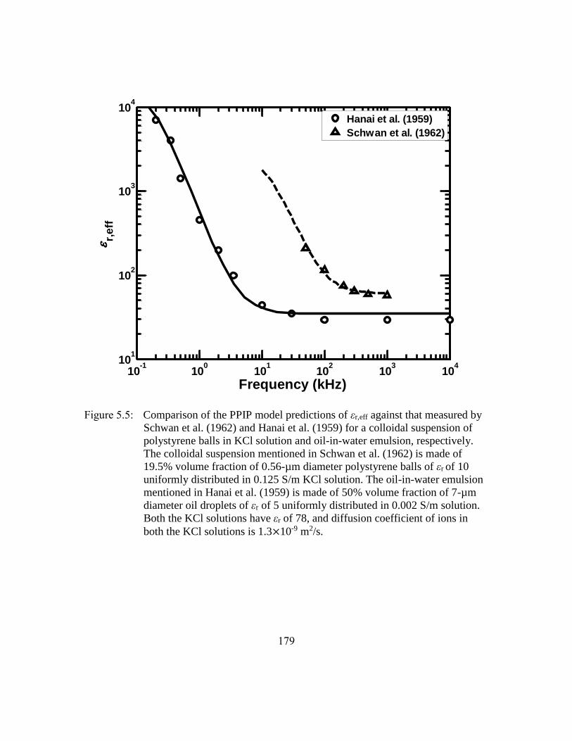
179

Figure 5.5: Comparison of the PPIP model predictions of εr,eff against that measured by

Schwan et al. (1962) and Hanai et al. (1959) for a colloidal suspension of

polystyrene balls in KCl solution and oil-in-water emulsion, respectively.

The colloidal suspension mentioned in Schwan et al. (1962) is made of

19.5% volume fraction of 0.56-µm diameter polystyrene balls of εr of 10

uniformly distributed in 0.125 S/m KCl solution. The oil-in-water emulsion

mentioned in Hanai et al. (1959) is made of 50% volume fraction of 7-µm

diameter oil droplets of εr of 5 uniformly distributed in 0.002 S/m solution.

Both the KCl solutions have εr of 78, and diffusion coefficient of ions in

both the KCl solutions is 1.3×10-9 m2/s.

10-1

100

101

102

103

104

101

102

103

104

Frequency (kHz)

r,

eff

Hanai et al. (1959)

Schwan et al. (1962)

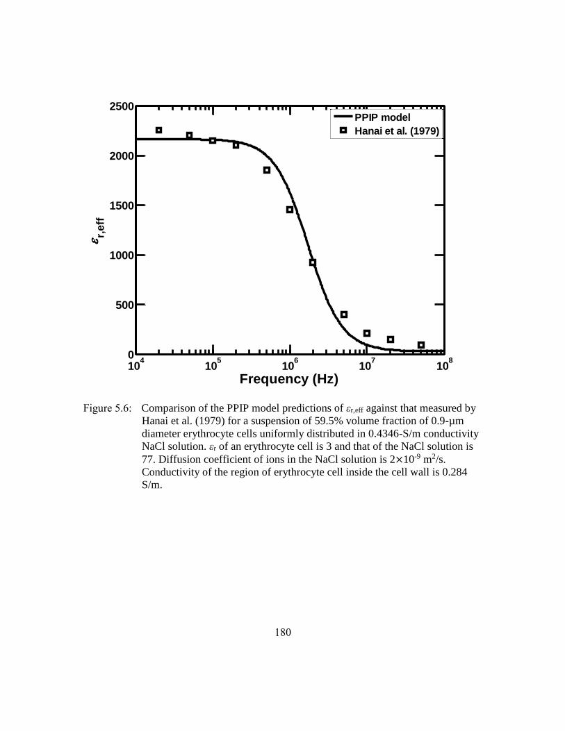
180


Hanai et al. (1979) for a suspension of 59.5% volume fraction of 0.9-µm

diameter erythrocyte cells uniformly distributed in 0.4346-S/m conductivity

NaCl solution. εr of an erythrocyte cell is 3 and that of the NaCl solution is

77. Diffusion coefficient of ions in the NaCl solution is 2×10-9 m2/s.

Conductivity of the region of erythrocyte cell inside the cell wall is 0.284

S/m.

104

105

106

107

108

0

500

1000

1500

2000

2500

Frequency (Hz)

r,

eff

PPIP model

Hanai et al. (1979)

181


Delgado et al. (1998) for two suspensions having 12.7% and 15.6% volume

fraction, respectively, of 115-µm diameter polymer latex balls uniformly

distributed in 0.0147-S/m conductivity KCl solution. εr of a latex ball is 15

and that of the KCl solution is 78. Diffusion coefficient of ions in the KCl

solution is 0.8×10-9 m2/s.

104

105

106

50

100

150

200

250

300

Frequency (Hz)

r,

eff

PPIP model (i=15.6%)

PPIP model (i=12.7%)

Delgado et al. (1998) (i=15.6%)

Delgado et al. (1998) (i=12.7%

182

Figure 5.8: Comparison of the PPIP-SCAIP model predictions of (a) resistivity (ρ) and

(b) phase angle (Θ) against that measured by Mahan et al. (1986) for

mixtures containing 80-µm diameter quartz grain matrix and uniformly

distributed 3.75% volume fraction of 276-µm diameter, 1000-S/m

conductivity chalcopyrite grains fully saturated with 34% volume fraction of

0.0094-S/m conductivity NaCl solution without any active ions. Comparison

of the PPIP-SCAIP model predictions of (c) resistivity (ρ) and (d) phase

angle (Θ) against that measured by Mahan et al. (1986) for mixtures

containing 80-µm diameter quartz grain matrix and uniformly distributed

5.8% volume fraction of 98-µm diameter, 5000-S/m conductivity pyrite

grains fully saturated with 37% volume fraction of 0.0094-S/m conductivity

NaCl solution with active ions. εr of chalcopyrite and pyrite is 10 and 15,

respectively, and that of the NaCl solution is 80. Diffusion coefficient of

charge carriers in chalcopyrite and pyrite is 10-7 and 10-6 m2/s, respectively,

and that of ions in the NaCl solution is 2×10-11 m2/s.

100

101

102

103

104

250

260

270

280

290

300

310

Frequency (Hz)

(

m)

(a)

100

101

102

103

104

0

20

40

60

80

Frequency (Hz)

-

(m

rad)

(b)

PPIP-SCAIP model

Mahan et al. (1986)

101

102

103

104

105

115

125

135

145

155

165

Frequency (Hz)

(

m)

(c)

101

102

103

104

105

0

20

40

60

80

100

120

Frequency (Hz)

-

(m

rad)

(d)

PPIP-SCAIP model

Mahan et al. (1986)

183


conductivity (σ′) and (b) quadrature conductivity (σ″) against that measured

by Abdel Aal et al. (2014) for two mixtures containing 0.3% volume

fraction of 5000-S/m conductivity pyrite inclusions of varying grain

diameter ranging from 0.075 to 0.15 mm and 0.15 to 0.3 mm, respectively.

Pyrite inclusions were uniformly distributed in porous sand matrix that is

fully saturated with 0.0256 S/m NaCl solution. εr of pyrite is 12 and that of

the NaCl solution is 80. Diffusion coefficient of charge carriers in pyrite is

10-6 m2/s and that of ions in the NaCl solution is 10-9 m2/s.

101

102

103

104

14

14.5

15

15.5

16

Frequency (kHz)

'

10

-3(S

/m)

(a)

101

102

103

104

0

4

8

12

16

20

Frequency (kHz)

"

10

-5(S

/m)

(b)

Est.0.02-0.15mm

Est.0.1-0.5 mm

Exp.0.075-0.15 mm

Exp.0.15-0.3 mm

184


conductivity (σ′) and (b) quadrature conductivity (σ″) against that measured

by Abdel Aal et al. (2014) for three mixtures containing 0.5%, 1%, and 2%

weight fraction, respectively, of 450-µm diameter pyrite inclusions

uniformly distributed in porous sand matrix fully saturated with 0.0256-S/m

conductivity NaCl solution. εr of pyrite is 12 and that of the NaCl solution is

80. Diffusion coefficient of charge carriers in pyrite is 10-6 m2/s and that of

ions in the NaCl solution is 10-9 m2/s.

101

102

103

104

12

13

14

15

16

Frequency (kHz)

'

10

-3(S

/m)

(a)

101

102

103

104

0

4

8

12

16

20

24

Frequency (kHz)

"

10

-5(S

/m)

(b)

Est. 2% w/w

Est. 1% w/w

Est. 0.5% w/w

Exp. 2% w/w

Exp. 1% w/w

Exp. 0.5% w/w

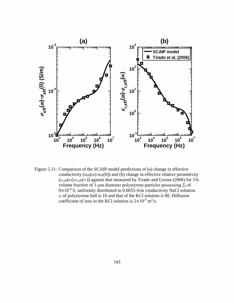
185

Figure 5.11: Comparison of the SCAIP model predictions of (a) change in effective

conductivity (σeff(ω)-σeff(0)) and (b) change in effective relative permittivity

(εr,eff(ω)-εr,eff(∞)) against that measured by Tirado and Grosse (2006) for 1%

volume fraction of 1-μm diameter polystyrene particles possessing Σs of

9×10-9 S, uniformly distributed in 0.0055-S/m conductivity NaCl solution.

εr of polystyrene ball is 10 and that of the KCl solution is 80. Diffusion

coefficient of ions in the KCl solution is 2×10-9 m2/s.

103

104

105

106

107

10-5

10-4

10-3

Frequency (Hz)

e

ff(

)-

eff(0

) (S

/m)

(a)

103

104

105

106

107

10-1

100

101

102

103

Frequency (Hz)

r,

eff(

)-

r,e

ff(

)

(b)

SCAIP model

Tirado et al. (2006)

186

Figure 5.12: Comparison of the PPIP model predictions of critical frequency of induced

frequency dispersion against that of Wong’s (1979) modeling results for

mixtures A and B containing conductive mineral inclusions of 5000-S/m

conductivity that are uniformly distributed in the electrolytic host medium.

Mixture A contains 8.3% volume fraction of conductive inclusions

distributed in the 0.002-S/m conductivity electrolytic host having diffusion

coefficient of ions of 10-9 m2/s. Mixture B contains 6% volume fraction of

conductive inclusions distributed in the 0.01-S/m conductivity electrolytic

host having diffusion coefficient of ions of 2×10-9 m2/s. For both the

mixtures, εr of conductive inclusion is 15 and that of the host is 12. Also, for

both the mixtures, the diffusion coefficient of charge carriers in the

conductive inclusions is 10-6 m2/s.

10-5

10-4

10-3

10-2

101

102

103

104

Radius (m)

Cri

tical F

req

uen

cy (

Hz)

PPIP Model

Wong (1979) A

Wong (1979) B

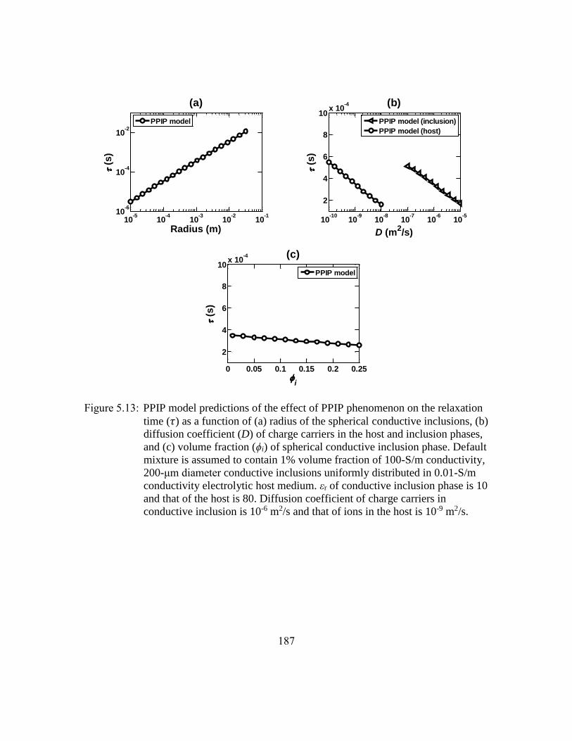
187

Figure 5.13: PPIP model predictions of the effect of PPIP phenomenon on the relaxation

time (𝜏) as a function of (a) radius of the spherical conductive inclusions, (b)

diffusion coefficient (D) of charge carriers in the host and inclusion phases,

and (c) volume fraction (ϕi) of spherical conductive inclusion phase. Default

mixture is assumed to contain 1% volume fraction of 100-S/m conductivity,

200-μm diameter conductive inclusions uniformly distributed in 0.01-S/m

conductivity electrolytic host medium. εr of conductive inclusion phase is 10

and that of the host is 80. Diffusion coefficient of charge carriers in

conductive inclusion is 10-6 m2/s and that of ions in the host is 10-9 m2/s.

10-5

10-4

10-3

10-2

10-1

10-6

10-4

10-2

Radius (m)

(

s)

(a)

PPIP model

10-10

10-9

10-8

10-7

10-6

10-5

2

4

6

8

10x 10

-4

D (m2/s)

(

s)

(b)

PPIP model (inclusion)

PPIP model (host)

0 0.05 0.1 0.15 0.2 0.25

2

4

6

8

10x 10

-4

i

(

s)

(c)

PPIP model

188

Figure 5.14: Comparison of the PPIP model predictions of chargeability (M) against that

estimated from various laboratory measurements of the complex resistivity

response of synthetic and geological samples for varying volume fractions

(ϕi) of conductive mineral inclusions in the range of (a) 0 to 8% and (b) 0 to

30% uniformly distributed in the host medium. (c) PPIP model predictions

of chargeability of mixtures containing varying volume fractions, in the

range of 0 to 25%, of conductive inclusions uniformly distributed in the host

medium for four different values of host conductivity. Default mixture is

assumed to contain 200-µm diameter conductive inclusions of 100-S/m

conductivity uniformly distributed in 0.01-S/m conductivity electrolytic host

medium. εr of the conductive inclusion phase is 10 and that of the host is 80.

Diffusion coefficient of charge carriers in conductive inclusion is 10-6 m2/s

and that of ions in the host is 10-9 m2/s.

0 0.02 0.04 0.06 0.080

0.1

0.2

0.3

0.4

0.5

i

M(a)

a=100 m (PPIP)

Wong (1979)

Hubbard et al. (2014)

Mahan et al. (1986)

De Witt (1979)

Florsch et al. (2011)

Pelton et al. (1978)

0 0.05 0.1 0.15 0.2 0.25 0.30

0.2

0.4

0.6

0.8

1

i

M

(b)

a=100 m (PPIP)

Wong (1979)

Hubbard et al. (2014)

Mahan et al. (1986)

De Witt (1979)

Florsch et al. (2011)

Pelton et al. (1978)

Gurin et al. (2013)

0 0.05 0.1 0.15 0.2 0.250

0.2

0.4

0.6

0.8

1

i

M

(c)

h=0.001 S/m

h=0.01 S/m

h=0.1 S/m

h=1 S/m

189

Chapter 6: Effects of Disseminated Conductive Mineral Inclusions on

Subsurface Electrical Measurements

Hydrocarbon-bearing conventional formations, mudrock formations, and source-

rock formations generally contain clays, pyrite, magnetite, graphite-like carbon, and/or

other electrically conductive mineral inclusions. Under redox-inactive conditions, these

inclusions give rise to perfectly polarized interfacial polarization (PPIP) when subjected to

an externally applied electric field. Effective electrical conductivity and dielectric

permittivity of geomaterials containing such inclusions are frequency-dependent

(dispersive) properties due to the electric-field-induced interfacial polarization and

associated charge relaxation processes around host-inclusion interfaces. Existing resistivity

interpretation techniques do not account for the effects of PPIP phenomena, and hence can

lead to inaccurate estimation of water saturation, total organic content, and conductivity of

formation water based on subsurface galvanic resistivity, EM induction, and EM

propagation measurements in geological formations containing conductive mineral

inclusions. In Chapter 5, I derived a mechanistic electrochemical model, the PPIP model,

and validated the PPIP-SCAIP model for purposes of quantifying the frequency-dependent

electrical complex conductivity of geomaterials. In this chapter, I use the PPIP-SCAIP

model to evaluate the dependence of effective complex-valued conductivity of geological

mixtures on (a) operating frequency, (b) conductivity of host medium (σh), and (c) material,

size, and shape of inclusion phase. Notably, I use the PPIP-SCAIP model to identify

petrophysical conditions that give rise to significant differences in effective conductivity

(σeff) and effective relative permittivity (εr,eff) of conductive-inclusion-bearing mixtures

from those of conductive-inclusion-free homogeneous media. I estimate that for a mixture

containing as low as 5% volume fraction of disseminated conductive inclusions, the low-

190

frequency effective conductivity of the mixture is in the range of -30% to +100% with

respect to the host conductivity for operating frequencies between 100 Hz and 100 kHz.

Further, the high-frequency effective relative permittivity of that mixture is in the range of

-10% to +90% with respect to the host permittivity for operating frequencies between 100

kHz and 10 MHz.

6.1 INTRODUCTION

Interfacial polarization phenomena significantly influence charge-carrier

migration, accumulation, and diffusion processes in geomaterials (Schmuck and Bazant,

2012). For a porous fluid-filled geomaterial containing conductive mineral inclusions,

charge carrier species in formation brine are ions, while those in conductive inclusions are

electrons and holes. In redox-inactive conditions, there is no charge transfer and charge

carrier transport across host-inclusion interfaces (Misra et al., 2015c). Consequently, these

interfaces are electrochemically inactive, possess negligible surface charges, and are

perfectly polarizable (Chu and Bazant, 2006).

Extensive studies have been carried out to describe interfacial polarization

phenomena arising from the effects of surface conductance (Σs) of surface-charge-bearing,

non-conductive spherical inclusions (e.g. Dukhin et al., 1974; Grosse, 1988). However,

laboratory investigations and numerical modeling work on interfacial polarization

phenomena arising from the effects of bulk conductivity of conductive mineral inclusions

disseminated in geomaterials are limited in the open literature (e.g. Misra et al., 2015b).

Anderson et al. (2006), Anderson et al. (2008), and, more recently, Wang and Poppitt

(2013) emphasize the need to model and measure the effects of interfacial polarization of

conductive inclusions for purposes of improving resistivity interpretation of subsurface

galvanic resistivity, EM induction, and EM propagation measurements. Existing resistivity

191

interpretation techniques for the three above-mentioned geo-electromagnetic

measurements neglect the effects of interfacial polarization of conductive mineral

inclusions (Anderson et al., 2007; Corley et al., 2010). Consequently, conventional

resistivity interpretation techniques tend to be inaccurate in pyrite-bearing sedimentary

rocks (Clavier et al., 1976; Altman et al., 2008), pyrite-bearing mudrocks (Misra et al.,

2015a), and organic source rocks that contain precursors to graphite (Anderson et al.,

2008).

Maxwell-Wagner, electrical-double-layer, and electrochemical polarization

phenomena occur in organic-rich mudrocks and source rock formations under the influence

of an externally applied electric field. Garrouch (1998) observed substantial differences in

measurements between wireline induction (~kHz) and LWD propagation (~MHz) tools in

clean-sand and shaly-sand formations due to Maxwell-Wagner and electrical-double-layer

polarization. Josh et al. (2012) observed that even at quite high frequencies up to 100s of

MHz, there is significant space-charge polarization effects in shale rocks. This behavior is

a consequence of the large surface area of clays and muds that carry surface charges. As a

result, the dielectric dispersion measurements in MHz to GHz frequency range are

significantly influenced by the volumetric content of brine and rock texture. Contrary to

several observations made in clean sands and shaly-sand formations, Josh (2014) observed

low correlation between high frequency dielectric permittivity (~GHz) and water content

of Schlattingen shales. Chen and Heidari (2014) demonstrated the effects of directional

connectivity of pyrite and organic matter on high frequency dielectric permittivity

measurements. They modified the CRIM model using a tortuosity-dependent coefficient to

obtain better fit with dielectric dispersion measurements in organic-rich mudrocks. Revil

et al. (2013) mentioned that tight-oil mudrock formations can be better characterized by

192

implementing an effective complex electrical conductivity model specific for shales and

mudrocks. According to them, such a model should incorporate the relative effects of

porosity, water saturation, kerogen content, conductive minerals, Maxwell-Wagner

polarization, clay types, clay content, and tortuosity tensor. Most importantly, Wang and

Poppitt (2013) produced first-of-its-kind continuous broadband subsurface

electromagnetic dispersion logging data. It was found that the measured X-signal

responses are as large as -30 mS/m and the inverted dielectric permittivity values are in the

order of 40000 in the pyrite-rich zones of the shale gas formations. They also emphasized

the need to develop a broadband electromagnetic dispersion interpretation methodology to

estimate petrophysical properties such as clay content, clay type, CEC, water salinity,

water-filled porosity, and kerogen content.

In this Chapter, I quantify the σeff and εr,eff of geomaterials containing uniformly

distributed conductive spherical, rod-like, and sheet-like inclusions by accounting for the

effects of PPIP phenomena. More importantly, petrophysical conditions that produce

significant differences between effective EM properties of geological mixtures and those

of conductive-inclusion-free, fluid-filled, porous host media are described in this chapter.

It is worth noting that the EM properties of conductive-inclusion-free, fluid-filled, porous

host media are vital to the accurate estimation of water saturation and total organic content,

but EM tools measure effective EM properties, which can be significantly different from

the EM properties of conductive-inclusion-free, fluid-filled, porous host media due to PPIP

phenomena. The PPIP model, one of the two models incorporated in the PPIP-SCAIP

model, quantifies the EM response of mixtures containing uncharged, perfectly polarizable

spherical, rod-like, and/or sheet-like conductive inclusions surrounded by either pore-

filling electrolyte or non-conductive matrix/fluid. On the other hand, the SCAIP model (the

193

second component of the PPIP-SCAIP model) quantifies the complex-valued conductivity

response of conductive-inclusion-free, fluid-filled, host media comprising spherical grains

that possess surface conductance.

6.2 COMPARISON OF THE PPIP-SCAIP MODEL TO EMPIRICAL MODELS

In this section, the PPIP model predictions are first compared against the SCAIP

model predictions of the low-frequency (LF) σeff and high-frequency (HF) εr,eff (Figure 6.1)

of conductive-inclusion-free mixtures comprising varying volume fractions of 1-mm

diameter, non-conductive spherical grains, possessing negligible surface conductance, that

are uniformly distributed in an electrolyte. Then, the PPIP-SCAIP model predictions are

compared against two well-established electrical model predictions of the LF σeff and HF

εr,eff (Figure 6.2) of conductive-inclusion-free mixtures comprising varying volume

fractions of 1-mm diameter, non-conductive spherical grains, possessing negligible surface

conductance, that are uniformly distributed in an electrolyte.

Figure 6.1 illustrates the LF σeff and HF εr,eff of three electrolyte-saturated,

conductive-inclusion-free mixtures W, S1 and S2 containing 0%, 20%, and 70% volume

fraction, respectively, of non-conductive spherical grains. Owing to the absence of

conductive inclusions and grains possessing surface conductance, none of the three curves

exhibit frequency dispersion in the LF σeff and HF εr,eff. Curve W, identifying 100% volume

fraction of 0.1-S/m conductivity water, indicates consistent LF σeff of 0.1 S/m and HF εr,eff

of 80. For curve S1, the LF σeff is reduced to 0.072 S/m and the HF εr,eff is reduced to 60

owing to the presence of 20% volume fraction of non-conductive spherical grains of low

relative permittivity. For mixture S2, containing 70% volume fraction of non-conductive

spherical grains, I observe further reduction in the LF σeff of the mixture to 0.022 S/m and

the HF εr,eff reduces to 22 due to reduction in interconnected electrolyte-filled porosity.

194

Curves W, S1, and S2 are generated using the PPIP model. These curves identify mixtures

comprising non-conductive spherical grains possessing no surface conductance.

Subsequently, curves W*, S1*, and S2* are generated using the SCAIP model for the three

above-mentioned mixtures, namely 0%, 20%, and 70% volume fraction, respectively, of

non-conductive spherical grains. Curves W*, S1*, and S2* identify mixtures comprising

non-conductive spherical grains possessing low values of Σs of 10-9 S (representative of Σs

of silica grains). As illustrated in Figure 6.1, the SCAIP model predictions are in good

agreement with the PPIP model predictions of the σeff and εr,eff of conductive-inclusion-free

mixtures comprising only non-conductive spherical grains and electrolyte. This agreement

is a consequence of the absence of conductive inclusions and grains possessing surface

conductance.

Figures 6.2a and 6.2b depict a good agreement between the computed LF σeff and

HF εr,eff values, respectively, with Archie’s model and Lichtenecker-Rother’s model (e.g.

Zakri et al., 1998), respectively. Despite the limitations of the PPIP-SCAIP model for non-

dilute mixtures containing volume fractions of inclusion phase greater than 20%, the

predictions of LF σeff and HF εr,eff using the two empirical models agree well with those of

the PPIP-SCAIP model. Assuming 100%-electrolyte-saturated mixture, Archie’s model

used for purposes of our comparison is described as

𝜎eff = 𝜎w(1 − 𝜙i)𝑚, (1)

where 𝜎w is the conductivity of electrolyte filling the pore space of the mixture, 𝜙i is

volume fraction of spherical non-conductive grains, and m is the porosity exponent of the

mixture. Experimental and numerical works have shown that the value of m is close to 1.3

for electrolyte-filled unconsolidated packs of non-conductive spherical grains (Jackson et

al., 2008; Revil and Skold, 2011). Accordingly, the PPIP-SCAIP model predicts that the

195

LF σeff of such mixtures agrees with the Archie’s model predictions for porosity exponent

value of 1.25, as shown in Figure 6.2a.

With respect to HF εr,eff of sand packs and other granular materials, experimental

investigations have shown that HF εr,eff can be modeled using Lichtenecker-Rother’s model

(Achour et al., 1999; Sabouroux and Ba, 2011), which is expressed as

(휀eff∗ )𝛼 = 𝜙i(휀i

∗)𝛼 + (1 − 𝜙i)(휀h∗)𝛼, (2)

where 휀eff∗ is effective complex-valued permittivity of the mixture, 휀i

∗ is complex-valued

permittivity of the non-conductive spherical grains, 휀h∗ is complex-valued conductivity of

the host medium comprising the pore-filling electrolyte, 𝜙i is volume fraction of spherical

grains, and the non-vanishing is the geometrical arrangement factor that ranges from -1

to 1 (Lee, 2010). The value of presents the relationship between the direction of effective

layering of the components to that of the applied electric field (Lee, 2010). When the

electric field is parallel to the composite layers, the value of = 1, giving a direct weighted

average of dielectric permittivity values of constituent phases, while when the field is

perpendicular to the composite layers, = -1 gives a harmonic weighing of the dielectric

permittivity values of individual phases (Leao et al., 2015). Moreover, Leao et al. (2015)

mention that when using = 1

3 in equation 2, one obtains Looyenga’s formula, whereas

= 1

2 reduces equation 2 to the CRIM model, which is suitable for isotropic homogeneous

media. The CRIM model has been extensively used to interpret high-frequency dielectric

measurements of geological formations (Seleznev et al., 2004; Hizem et al., 2008). In

Figure 6.2b, our mechanistic model predictions of the HF εr,eff of electrolyte-saturated

mixtures comprising different volume fractions of uncharged, non-conductive spherical

grains agree with Lichtenecker-Rother’s model predictions for = 0.69. Values of of

0.66 and 0.7 are reported in the literature survey by Lee (2010). The agreement of PPIP-

196

SCAIP model predictions with the two empirical electrical models, as shown in Figure 6.2,

supports the mechanistic and mathematical robustness of the improved modeling scheme

discussed in this work.

6.3 COMPLEX ELECTRICAL CONDUCTIVITY RESPONSE OF GEOMATERIALS

CONTAINING DISSEMINATED INCLUSIONS

In this section, the complex-valued conductivity response of mixtures containing

uniformly distributed inclusions is modeled using the PPIP model. In doing so, I identify

petrophysical properties that govern PPIP phenomena around conductive inclusions. In the

first half of this section, I study the interfacial polarization of conductive spherical

inclusions in absence of redox-active species. Unlike those in previously published

research works (Wong, 1979; Placencia-Gomez and Slater, 2014), the inclusion phase in

this wrok are assumed to be finitely conducting with inherent dielectric properties; similar

considerations were made by Revil et al. (2015a). Additionally, I study the sensitivity of

complex-valued conductivity to the dispersity of inclusion sizes (Beltramo and Furst,

2012), distribution of inclusion sizes (Arroyo et al., 1999), and material of the inclusion

phase. In the latter half of this section, I model PPIP phenomena around conductive sheet-

like and rod-like inclusions. Numerical studies of interfacial polarization phenomena

around conductive inclusions of such shapes for applications in geosciences are limited in

the open literature (e.g. Grosse, 1988; Sihvola, 2007). All model predictions reported in

this section are supported by theoretical explanations based on first principles.

6.3.1 Material of Inclusion Phase

In this study, the inclusion phase differs in its conductivity, relative permittivity,

and diffusion coefficient of charge carriers. Figure 6.3 depicts the computed σeff and εr,eff

responses of mixtures containing spherical inclusions of different materials. In that figure,

197

curves G, P, C, X, Y, and H identify six mixtures containing only graphite inclusions, pyrite

inclusions, chalcopyrite inclusions, low-conductivity material inclusions, 0.1-S/m

conductivity inclusions, and non-conductive inclusions, respectively, uniformly distributed

in a 0.1-S/m conductivity electrolyte. The assumed values of conductivity, relative

permittivity, and diffusion coefficient of charge carriers of these six materials are reported

in Table 6.1.

I observe significant dispersion in the computed σeff and εr,eff responses of mixtures

G, P, C, and Y. Also, Figure 6.3b shows large dielectric enhancements in the low-frequency

limits for all the mixtures except mixture H. Interestingly, Figure 6.3a shows that LF σeff

values of all mixtures converge to a value lower than the σh of 0.1 S/m, which results from

the dielectric behavior of conductive inclusions with perfectly polarizable surfaces at low

frequencies. Similar reduction in the LF σeff values below σh were observed by Revil et al.

(2015b). Conductive inclusions behave as dielectric material at low frequencies (< 1 kHz)

owing to charge accumulation at the host-inclusion interfaces. On the other hand, the HF

σeff of mixtures G, P, and C converge to a value higher than σh, which is indicative of the

high conductivity behavior of such inclusions at higher frequencies. Another interesting

feature shown in Figure 6.3a is that for mixture Y, containing 0.1-S/m conductivity (equal

to σh) inclusions, the HF σeff values are equal to σh, whereas the LF σeff values are much

lower than σh due to the accumulation of charges at the electrochemically inactive surfaces

of these inclusions in accordance with PPIP model assumptions. In contrast, in Figure 6.3b

mixture H, containing non-conductive inclusions, exhibits a non-dispersive EM response

due to the absence of interfacial polarization.

From a theoretical stand point, an increase in the metallic nature of inclusion

material implies an increase in the concentration of charge carriers and an increase in the

198

mobility of charge carriers in the inclusion phase. In this study, mixture G contains

inclusions of the highest metallic nature followed by mixture P and then mixture C (e.g.

Pridmore and Shuey, 1976). Among the mixtures used in our study, mixture G undergoes

the highest accumulation of charges around the host-inclusion interfaces at low frequencies

due to the highest charge carrier concentration, thereby giving rise to largest dielectric

enhancement and largest LF εr,eff, as shown in Figure 6.3b. Moreover, mixture G exhibits

higher HF σeff than those of mixtures P and C, as illustrated in Figure 6.3a, because graphite

inclusions have higher mobility and concentration of charge carriers. It is noteworthy that,

an increase in the metallic nature of the disseminated inclusion phase results in faster

alignment of the field-induced polarization with the externally applied electric field,

whereupon the frequency dispersion for mixture G occurs at much lower frequencies than

those of mixtures P and C (e.g. Pelton et al., 1978; Gurin et al., 2015).

Figures 6.3a and 6.3b show an intuitive conductivity response wherein the σeff of

the graphite mixture is higher than that of the pyrite mixture, which in turn is higher than

that of the chalcopyrite mixture over the entire frequency range. However, Figure 6.4a

illustrates a counter-intuitive conductivity response, wherein mixtures G, P, and C exhibit

similar σeff responses, despite dissimilarities in the metallic nature of the inclusion

materials. I claim that this counterintuitive behavior is a consequence of the equal ratio of

the conductivity of inclusion phase to the diffusion coefficient of charge carriers in the

inclusion phase for the three mixtures, as shown in the last column of Table 6.2.

Nonetheless, the PPIP model predictions in Figure 6.4a indicate that mixtures containing

conductive inclusions of bulk conductivity values close to or lower than 1 S/m, for instance

mixtures X and Y, the σeff responses diverge from the counter-intuitive converging

responses, as exhibited by mixtures G, P, and C.

199

Organic-rich and hydrocarbon-bearing geological rocks typically contain more than

one type of conductive mineral inclusions. In this section, the complex-valued conductivity

response of mixtures containing uniformly distributed conductive inclusions of one or more

different type of materials is quantified using the PPIP-SCAIP model. Figure 6.5 shows

the modeled EM response of various mixtures containing 70% volume fraction of 100-μm

diameter non-conductive spherical grains mixed with various volume fractions of 100-μm

diameter, conductive inclusions of one or more types of materials uniformly distributed in

a 0.1-S/m electrolyte. In Figure 6.5, the computed EM responses of four mixtures, namely

mixtures S, G, P, and C, are provided as references to compare the effects of the presence

of more than one type of materials as the inclusion phase. Mixtures S, G, P, and C identify

mixtures containing no inclusions, only 2% volume fraction of graphite inclusions, only

2% volume fraction of pyrite inclusions, and only 2% volume fraction of chalcopyrite

inclusions, respectively. In Figure 6.5a, mixture S, which contains no conductive

inclusions, exhibits a non-dispersive response that agrees with Archie’s prediction. Further,

mixtures G, P, and C, which contain conductive inclusions of different type of materials,

give rise to significantly distinct Θ responses, owing to the dissimilarity in the metallic

nature of the materials (Gurin et al., 2015). For example, Figure 6.5b illustrates that the

peak of the Θ response of mixture G is at 5 kHz, that of mixture P is at 20 kHz, and that of

mixture C is at 50 kHz.

On the other hand, mixture CG, which was obtained by mixing 2% volume fraction

of graphite with 2% volume fraction of chalcopyrite, exhibits a Θ response having two

peaks corresponding to the constituent materials of the inclusion phase in the resulting

mixture. Interestingly, the Θ responses of mixtures containing inclusions of two or more

materials are broader than those of mixtures containing inclusions of only one material.

200

Further, mixtures containing inclusions of two different materials that are not significantly

different in their electrical properties and metallic nature show only a single peak in the Θ

response. For instance, the Θ response of mixture PG, which contains a 2% volume fraction

of graphite inclusions and a 2% volume fraction of pyrite inclusions, exhibits only a single

peak. Furthermore, for mixture CPG, which contains a 2% volume fraction of inclusions

of each of the three materials, namely chalcopyrite, pyrite, and graphite, I observe a sharp

frequency dispersion in the conductivity response (Figure 6.5a), a broad single-peak Θ

response (Figure 6.5b), and a significant difference in LF and HF effective conductivity

(Figure 6.5a), corresponding to the increase in volume fraction of conductive inclusions

due to the volumetric mixing in equal concentrations.

6.3.2 Dispersed clay particles v/s conductive mineral inclusions

In this section, I compare the EM response of mixtures containing non-conductive

particles possessing surface conductance, which identify clay minerals, clay-sized

particles, and silt-sized particles, against that of mixtures containing conductive/semi-

conductive inclusions, which identify pyrite and magnetite inclusions. Clay minerals, clay-

sized particles, and silt-sized particles have negligible bulk conductivity and possess

surface charges that give rise to surface conductance (Revil, 2012). In contrast,

conductive/semi-conductive metallic mineral inclusions possess high bulk conductivity

without surface charges under redox inactive conditions (Chu and Bazant, 2006). Clay-like

minerals undergo surface-conductance-assisted interfacial polarization phenomena that

follow a significantly different mechanisms than those of semi-conductive/conductive

minerals, which undergo perfectly polarized interfacial polarization under redox-inactive

conditions (Misra et al., 2015c). In Figure 6.6b, PPIP-SCAIP model predictions indicate

that mixtures containing conductive inclusions exhibit dispersion responses that are

201

markedly distinct from those of mixtures containing non-conductive inclusions possessing

surface conductance. Mixtures P and G, which contain 2% volume fraction of uniformly

distributed conductive pyrite and graphite inclusions, respectively, exhibit much larger

peaks of the Θ response than that of mixture Cl2, which contains 10% volume fraction of

uniformly distributed non-conductive spherical grains possessing Σs of 10-8 S, identifying

a shaly sand. Moreover, mixture Cl1, which contains 70% volume fraction of uniformly

distributed non-conductive spherical grains possessing Σs of 10-8 S (identifying a mudrock)

exhibits a significantly lower peak in its Θ response than those of mixtures P and G.

As shown in Figure 6.6b, the critical frequency of mixture P is at 3 kHz and that of

mixture G is at 1 kHz, which is approximately two orders of magnitude higher than those

of mixtures Cl1 and Cl2 of 50 Hz. Such differences in peaks of the Θ responses were

predicted by Anderson et al. (2006) and in their subsequent papers. Also, comparisons of

experimental observations made by Jougnot et al. (2010) on clay rocks against those made

by Gurin et al. (2015) on mixtures containing electronic conductors support our model

predictions. Significant variations in the peak and critical frequency of the Θ response are

due to the difference in SCAIP and PPIP phenomena. The dispersive Θ response of

mixtures containing non-conductive inclusions possessing surface conductance is

dominant at frequencies between 1 Hz and 100 Hz (Shilov and Borkovskaya, 2010). On

the other hand, mixtures containing metallic inclusions have a dominant dispersive

response in the 1-50 kHz frequency range (Wong, 1979; Grosse and Barchini, 1992).

The PPIP-SCAIP model predictions, as shown in Figure 6.6, indicate that at

operating frequencies of downhole induction logging tools in the range of 1 kHz to 50 kHz,

the EM response will be substantially influenced by interfacial polarization of conductive

mineral inclusions and relatively unaffected by the interfacial polarization of clay-like

202

inclusions. However, at operating frequencies of galvanic resistivity tools around 100 Hz,

the EM response is influenced by interfacial polarization of both clay-like inclusions and

conductive mineral inclusions. Figure 6.6a illustrates that presence of 10% volume fraction

dispersed clays, as in mixture Cl2, will lower σeff to values smaller than σh in the entire

frequency range of 1 Hz to 1 MHz. Moreover, presence of 2% volume fraction of pyrite

inclusions, as in mixture P, or graphite inclusions, as in mixture G, gives rise to frequency

dispersion of conductivity responses in the frequency range of 1 Hz to 1 MHz, wherein the

LF σeff values are substantially lower and the HF σeff values are substantially higher than

the conductivity of the host medium. Further, mixture Cl1 identifying with a mixture

containing 70% volume fraction of clay-like particles possessing Σs of 10-8 S, exhibits

120% higher σeff values than that of inclusion-free mixture S, due to the effects of surface

conductance of clay-like particles present at a high volumetric concentration.

6.3.3 Size of inclusions

Relaxation mechanisms associated with PPIP phenomena strongly depend on the

surface area (or the characteristic length) of the disseminated conductive inclusion phase.

In this section, I investigate the influence of inclusion size, distribution of inclusion sizes,

and dispersity of inclusion sizes on the EM response of mixtures containing 10% volume

fraction of 500-S/m conductivity spherical inclusions uniformly distributed in a 0.01-S/m

conductivity electrolyte. Figure 6.7 illustrates that the frequency dispersion curve shifts

toward higher frequencies by approximately an order of magnitude for every order of

magnitude reduction in the size of inclusions. Peaks of the Θ responses for mixtures M1,

M2, and M3, which contain 10-µm, 100-µm, and 1000-µm diameter conductive spherical

inclusions, respectively, are at 12 kHz, 1.2 kHz, and 0.12 kHz, respectively. From a

theoretical standpoint, at a constant volume fraction of conductive inclusions, a decrease

203

in size of conductive inclusions in the mixture results in faster build-up of charge

accumulation at interfaces. Therefore, interfacial polarization of smaller-sized inclusions

follows the time-varying externally applied electric field at higher frequencies;

consequently, the frequency dispersion of a mixture containing smaller-sized inclusions

appears at higher frequencies than that of a mixture containing larger-sized inclusions.

Figure 6.7 illustrates the EM response of mixtures M4 and M5, which contain conductive

spherical inclusions with a uniform distribution of sizes (90% variation) about a mean

diameter of 10 µm varying from 1 to 19 µm and that about a mean diameter of 100 µm

varying from 10 to 190 µm, respectively. The magnitudes of peaks of the Θ responses of

mixtures M4 and M5, which have variations in sizes of the inclusions, decreases by

approximately 10% with respect to those of mixtures M1 and M2, which have uniform

sizes of inclusions. However, the critical frequency remains nearly unchanged for mixtures

M1 and M4 and for M2 and M5.

Instead of being a monodisperse mixture, a geological mixture can be bidisperse or

polydisperse. Figure 6.8 illustrates the computed complex-valued conductivity response of

mixtures containing more than one size (dispersivity) of conductive inclusions. The Θ

response of the bidisperse mixture M7, which contains 5% volume fractions of 10-µm and

1000-µm diameter conductive spherical inclusions, respectively, exhibits two distinct

peaks, as shown in Figure 6.8b, owing to the two sizes of inclusions present in the mixture

that are more than an order of magnitude different from each other. However, the Θ

response of mixture M6, which contains 5% volume fractions of 10-µm and 100-µm

diameter conductive spherical inclusions, respectively, exhibits two peaks that are closely

spaced and can be distinguished only through a high-resolution spectral measurement.

Further, Figure 6.8b shows that the polydisperse mixture M8, which contain 3.33% volume

204

fractions of 10-µm, 100- µm, and 1000-µm diameter conductive spherical inclusions,

respectively, exhibits broader Θ responses than those of mixtures containing monodisperse

and bidisperse inclusion sizes. Similar behavior is also exhibited by mixture M9, which

contains 2.5% volume fractions of 1-µm, 10-µm, 100- µm, and 1000-µm diameter

conductive spherical inclusions, respectively. Also, Figure 6.8a indicates that an increase

in the dispersivity of inclusion sizes leads to an increase in the spread and decrease in

steepness of conductivity dispersion. Interestingly, the magnitude of the peak of the Θ

response is higher for mixtures containing inclusions of sizes that are less than an order of

magnitude different from each other; for instance, the magnitude of the peak of the Θ

response of mixture M6 is higher than that of mixture M7, as shown in Figure 6.8b.

6.3.4 Laminations, veins, fractures, and beds

In this and the next section, I model the EM responses of mixtures containing sheet-

like and rod-like conductive inclusions, respectively. To the best of our knowledge, PPIP

phenomena around uniformly distributed rod-like and sheet-like inclusions have not been

investigated for purposes of petrophysical applications. Beds, laminations, pore-filling

mineralization, fractures, and veins typically present in geological mixtures are comparable

to the two inclusion geometries under investigation in this and the next section.

PPIP model predictions indicate that the complex-valued conductivity response of

mixtures containing conductive sheet-like inclusions (e.g., thin-beds and laminations)

strongly depends on σh. In Figures 6.9a and 6.9b, frequency dispersion shifts to higher

frequencies with an increase in conductivity of the electrolytic-host medium. An increase

in the conductivity of electrolyte surrounding the inclusion increases the number of ions in

the electrolyte, which in turn increases charge accumulation at the outer surface of the

inclusions, resulting in an increase in phase at low frequencies. Consequently, in Figure

205

6.9b, the LF Θ response at 10 Hz is highest for the mixture having a 1-S/m conductivity

host. Additionally, the field-induced polarization of sheet-like inclusions follows the

applied electric field until higher frequencies for mixtures having higher host conductivity

owing to the greater mobility of charge carriers (ions) in the electrolytic host, which easily

accumulate at the outer surface under the combined influence of dipole moment of the

inclusion and the externally applied electric field and generate complete polarization.

Unlike the behavior of mixtures containing spherical and rod-like inclusions, a mixture

containing sheet-like inclusions under redox-inactive conditions acts as an insulator at low

frequencies. Therefore, for sheet-like conductive inclusions, the LF σeff values are close to

zero and the LF Θ values are close to 90-degrees for the mixture having a 1-S/m

conductivity host, which indicates the perfect dielectric behavior of that mixture.

The thickness of sheet-like inclusions significantly affects the EM response of

mixtures containing such inclusions. In Figures 6.9c and 6.9d, the frequency dispersion

characteristics shift to higher frequencies with a decrease in the thickness of sheet-like

inclusions. Irrespective of the thickness, all the curves in Figure 6.9c exhibit similar LF

and HF limits for the σeff and Θ values, which honors the mixing law predictions for

insulating and infinitely conductive behavior of sheet-like inclusions at low (~ Hz) and

high frequencies (~ GHz), respectively. PPIP model predictions in Figure 6.9c indicate that

2 mm or thicker beds uniformly distributed in geological host will not exhibit dispersion

characteristics for frequencies higher than 100 Hz. As a result, subsurface EM induction

and EM propagation measurements can be interpreted using laminated sand analysis when

the thickness of disseminated parallelly aligned sheet-like inclusions is greater than or close

to 2 mm. However, for accurate well-log interpretation in thinly laminated systems

206

(thickness < 1 mm), the effects of PPIP phenomena should be accounted when quantifying

the frequency dispersion of the σeff and Θ responses.

Finally, Figure 6.9f shows that the magnitude of the Θ response increases with an

increase in the volume fraction of sheet-like inclusions. In Figures 6.9e and 6.9f, for a

mixture containing 1% volume fraction of sheet-like inclusions, the Θ response is

negligible and σeff values are close to σh, respectively. However, for a mixture with higher

volume fractions of sheet-like inclusions, the complex-valued conductivity response

exhibits drastic alteration in both the Θ and σeff responses, as illustrated in Figures 6.9e and

9f. Also, the HF σeff response of mixtures containing sheet-like inclusions increases with

an increase in volume fraction of the inclusion phase in accordance with mixing law

predictions. As demonstrated by the explanation provided in the earlier part of this section,

an increase in volume fraction of sheet-like inclusions in the mixture leads to a decrease in

the LF σeff response of the mixture, as illustrated in Figures 6.9e.

6.3.5 Pore-throat-filling and rod-like mineralization

In this section, I focus on mixtures containing uniformly distributed, parallelly

aligned, rod-like inclusions. In Figures 6.10a and 6.10b, the frequency dispersion response

of rod-like inclusions is significantly different from those of sheet-like inclusions shown

in the previous section. At low frequencies (~ Hz), charge carriers in the uniformly

distributed rod-like inclusions accumulate at host-inclusion interfaces and migration of

charge carriers only occurs in the electrolytic host medium. Also, displacement currents

are much smaller than conduction currents at low frequencies. Nonetheless, the Θ response

of such mixtures strongly depends on σh, as shown in Figure 6.10b. Mixtures having a

low-conductivity host exhibit frequency dispersion at low frequencies. Such dispersion

characteristics shift to higher frequencies with an increase in σh. It is important to remember

207

that the εr,eff (the charge storage potential) of these mixtures decreases with an increase in

operating frequency. The Θ response of mixtures being a ratio of displacement current to

conduction current, a minimum follows a maximum Θ response. Interestingly, in Figure

6.10b the magnitude of the peak of the Θ response is almost equal for all the different

values of σh.

In Figures 6.10c and 6.10d mixtures containing larger diameter rod-like inclusions

exhibit frequency dispersion at much lower frequencies than those containing smaller

diameter inclusions. Consequently, mixtures containing smaller-diameter rod-like

inclusions will exhibit lower conductivity values than those containing larger-diameter rod-

like inclusions for a considerably larger frequency range. This behavior is attributed to the

relatively shorter distances that charge carriers in the inclusion phase are required to travel

inside the smaller-diameter inclusions. Consequently, mixtures containing smaller

diameter inclusions undergo complete polarization of inclusions for much higher

frequencies and exhibit lower values of σeff. Also, in Figure 6.10d, the magnitude of the

peak of the Θ response is relatively independent of the diameter of rod-like inclusions.

Finally, Figure 6.10e shows that, at a 5% volume fraction of rod-like inclusions, the

frequency dispersion in σeff results in LF σeff values 10% lower and HF σeff values 10%

higher than σh, in accordance with mixing law predictions. Moreover, in Figure 6.10f, the

magnitude of the peak of the Θ response increases with an increase in volume fraction of

rod-like inclusions, while the critical frequency associated with the peak of the Θ response

remains relatively unaltered.

208

6.4 EFFECTS OF PPIP AND SCAIP PHENOMENA ON SUBSURFACE ELECTRICAL

MEASUREMENTS

Petrophysicists and geoscientists typically interpret EM measurements of low-

frequency electrical conductivity, high-frequency conductivity phase and attenuation, and

high-frequency dielectric permittivity of inclusion-free geological samples to assess water

saturation, total organic content, formation electrical anisotropy, formation water salinity,

and other electrical properties. They employ galvanic resistivity (e.g., laterolog

measurements) and EM induction methods (e.g., array induction measurements) to assess

the LF conductivity of formations, EM propagation methods for measuring high-frequency

phase and attenuation of formations, and dielectric methods for measuring high-frequency

permittivity of formations. However, when a porous geological host contains inclusions in

the form of grains, vugs, patches, pore throat-filling structures, fractures, and/or

laminations, the accumulation/depletion and relaxation of charges around host-inclusion

interfaces significantly alter the electromigration, charge storage, and electrodiffusion

processes in the host medium. As a result, resistivity interpretation techniques that do not

account for the effects of PPIP phenomena lead to inaccurate assessment of petrophysical

properties of geological formations. The PPIP-SCAIP model quantifies the alteration of

EM measurements due to SCAIP and PPIP phenomena. In this section, I use the PPIP

model to identify the petrophysical conditions that lead to significant alterations of galvanic

resistivity, EM induction, and EM propagation measurements in the frequency range from

100 Hz to 100 MHz.

The computed EM response of each mixture is presented as two set of plots, namely

effective conductivity (σeff) plot and effective relative permittivity (εr,eff) plot. All σeff plots

are depicted for low frequency measurements that range from 0.1 kHz to 100 kHz. All εr,eff

plots are depicted for high frequency measurements that range from 1 MHz to 100 MHz.

209

Consequently, curves presented in the σeff plot are comparable to LF σeff estimates based

on galvanic resistivity and EM induction measurements. On the other hand, curves

presented in the εr,eff plot are comparable to HF εr,eff estimates based on EM propagation

and dielectric propagation measurements. For all the plots, a non-dispersive response of

the inclusion-free mixture S is presented as a reference curve for visualizing the severity

of alterations due to the presence of conductive inclusions. When the LF σeff and HF εr,eff

responses of a mixture deviate from the reference curve, it indicates that conventional

resistivity interpretation of galvanic resistivity, EM induction, and EM propagation

measurements in formations similar to the mixture will not yield accurate petrophysical

assessments. Unlike other previous works on modeling interfacial polarization phenomena

(Wong, 1979; Mahan et al., 1986), I ensure petrophysically consistent modeling by

coupling the SCAIP model to the PPIP model, thereby quantifying the effects of

polarization due to the background material (matrix) made of non-conductive grains

possessing surface conductance and those due to the perfectly polarizable inclusions

uniformly distributed in the mixture.

6.4.1 Shape of inclusions and conductivity of pore-filling fluid

Pyrite mineralization tends to be associated with hydrocarbon bearing formations,

sedimentary rocks, and source rocks. In this section, I assign electrical properties to the

inclusion phase comparable to that of conductive pyrite mineral. For the inclusion phase,

the assumed value of bulk conductivity is 5000 S/m, relative permittivity is 12, and the

diffusion coefficient of charge carriers in the inclusion phase is 5×10-5 m2/s. Moreover, the

assumed value of relative permittivity of non-conductive spherical grains, identifying a

sand grains, is 4 and that of non-conductive spherical grains, identifying clay grains, is 8.

210

The assumed value of Σs of representative sand grains is 10-9 S and that of the representative

clay grains is 10-8 S.

Figure 6.11 shows the computed EM response of mixtures SP1, SP2, and SP3

containing 5% volume fraction of conductive inclusions in shape of either 200-μm diameter

spherical grains, 20-μm diameter long rods, or 1-mm thick sheets, respectively, uniformly

distributed in a matrix made of 70% volume fraction of 1-mm diameter, non-conductive

spherical grains that is completely saturated with electrolyte for various electrolyte

conductivities. I also present the computed EM response of a mixture SCl made of 70%

volume fraction of 1-mm diameter, non-conductive spherical grains containing uniformly

distributed 5% volume fraction of 10-μm diameter, non-conductive spherical grains

possessing Σs of 10-8 S that is fully saturated with electrolyte for various electrolyte

conductivities. The computed EM response of the inclusion-free mixture S containing only

70% volume fraction of non-conductive spherical grains exhibiting a low value of Σs of 10-

9 S is presented as a reference to visualize the alteration of the EM response due to PPIP

effects. Pairs of Figures 6.11a and 6.11b, 6.11c and 6.11d, 6.11e and 6.11f, and 6.11g and

6.11h identify the computed σeff and εr,eff responses of mixtures, respectively, fully

saturated with 0.001-, 0.01-, 0.1-, and 1-S/m electrolyte, respectively. It is important to

note that the computed EM responses shown in Figure 6.11 are along the direction of

characteristic length of the inclusion phase.

Important observations regarding the LF σeff response are as follows:

(1) Mixtures SP1, SP2, and SP3 undergo significant variations of the LF σeff and HF

εr,eff responses with respect to that of the inclusion-free mixture S.

(2) The variations of LF σeff and HF εr,eff responses with respect to the reference curve

strongly depend on the conductivity of pore-filling electrolyte because the frequency

211

dispersion characteristics of a mixture shift to lower frequencies with a decrease in the

electrolyte conductivity, as emphasized in previous sections.

(3) For mixtures SP1 and SP2, the variation of LF σeff with respect to the reference

curve and frequency dispersion of the LF σeff increases with a decrease in electrolyte

conductivity.

(4) In the operating frequency range of a typical galvanic resistivity measurement (~

100 Hz), the variations of LF σeff responses of mixtures SP1 and SP2 with respect to

reference curves are independent of electrolyte conductivity for electrolyte

conductivity values higher than or close to 0.01 S/m, as shown in Figures 6.11c, 6.11e,

and 6.11g.

(5) The variation of the LF σeff with respect to the reference curve strongly depends on

the shape of inclusions.

(6) For electrolyte conductivity values higher than or close to 0.01 S/m, mixture SCl

exhibits LF σeff values that are lower than that of inclusion-free mixture S, as shown

in Figures 6.11c, 6.11e, and 6.11g, because surface conduction is negligible compared

to bulk conduction. However, for electrolyte conductivity values lower than or close

to 0.001 S/m, the LF σeff values of mixture SCl are higher than that of the inclusion-

free mixture S, as illustrated in Figure 6.11a, because surface conduction dominates

bulk conduction. Similar increases in conductivity values in the presence of low

conductivity electrolytes around clay grains have been extensively reported in the

published petrophysical literature (e.g., Waxman and Smits, 1968).

(7) In the operating frequency range of the EM induction measurements (~ 50 kHz),

the LF σeff increases by 96%, 51%, and 38% with respect to that of inclusion-free

212

mixture S for mixtures SP1, SP2, and SP3, respectively, owing to the effects of PPIP

phenomena.

(8) As illustrated in Figures 6.11c, 6.11e, and 6.11g, for electrolyte conductivity values

higher than or close to 0.01 S/m and frequencies close to a typical galvanic resistivity

measurements operating at 100 Hz, mixtures SP1 and SP2 exhibit LF σeff values that

are approximately 20% lower than that of inclusion-free mixture S.

(9) Mixture SP3 exhibits an extremely large reduction of LF σeff values with respect to

that of inclusion-free mixture S at frequencies close to 100 Hz and electrolyte

conductivity values close to or higher than 1 S/m because sheet-like inclusions act as

insulators at low frequencies and high values of electrolyte conductivities, as shown

in Figure 6.11g.

(10) As illustrated in Figures 6.11a, 6.11c, and 6.11e, for electrolyte conductivity

values lower than or close to 0.1 S/m, mixture SP3 exhibits negligible frequency

dispersion in the LF σeff response and approximately 96% higher values of LF σeff than

that of inclusion-free mixture S.

Additional important observations regarding the HF εr,eff response are as follows:

(1) As shown in Figures 6.11b, 6.11d, and 6.11f, for electrolyte conductivity values

close to or lower than 0.1 S/m, the HF εr,eff of mixtures SP1, SP2, and SP3 are 76%,

43%, or 33% higher, respectively, than that of the inclusion-free mixture S.

(2) Mixtures SP1, SP2, and SP3 exhibit a non-dispersive HF εr,eff response for

electrolyte conductivity values close to or lower than 0.01 S/m, as shown in Figures

6.11b and 6.11d.

(3) Mixture SCl exhibits a non-dispersive HF εr,eff response for electrolyte conductivity

values in the range of 0.001 S/m to 1 S/m.

213

(4) With an increase in electrolyte conductivity, the frequency dispersion of HF εr,eff

response is observable due to the shift of dispersion characteristics to higher

frequencies resulting in an increase in HF εr,eff, as shown in Figures 6.11f and 6.11g.

(5) As shown in Figures 6.11f and 6.11h, for electrolyte conductivity values close to or

higher than 0.1 S/m, HF εr,eff values at frequencies close to 100 MHz are relatively

independent of the change in electrolyte conductivity, whereas large variations in the

HF εr,eff response with respect to the reference curve are observed for frequencies close

to or lower than 1 MHz.

6.4.2 Non-conductive pore-filling fluid

Figure 6.12 illustrates the computed EM response of various mixtures having non-

conductive pore-filling fluid of bulk relative permittivity of 3, which identifies with

hydrocarbon. Figure 6.12 shows that the LF σeff and HF εr,eff of mixtures SP1, SP2, and

SP3 are all approximately 27% and 12% higher, respectively, than those of the inclusion-

free mixture S. There is negligible frequency dispersion of HF εr,eff for these mixtures, as

illustrated in Figure 6.12b. In contrast, mixture SCl exhibits frequency dispersion of HF

εr,eff and LF σeff at frequencies higher than 10 kHz. Mixtures SP1 and SP2 containing

spherical and rod-like pyrite inclusions, respectively, exhibit LF σeff responses that are

nearly similar to that of mixture SCl, while the mixture SP3 containing sheet-like

inclusions exhibit higher LF σeff values.

6.4.3 Volume content of inclusion phase

Interfacial polarization is a surface governed phenomenon that strongly depends on

the volume content of inclusions in the mixture. Figure 6.13a shows that the LF σeff of the

two SP3-type mixtures containing 1% volume fraction (dotted) and 2% volume fraction

214

(solid), respectively, of sheet-like conductive inclusions are 27% and 49% higher than that

of the inclusion-free mixture S, respectively. These mixtures containing sheet-like

inclusions exhibit negligible dispersion characteristics in the LF σeff response. At

frequencies close to 100 Hz, the LF σeff responses of one SP1-type mixture containing 2%

volume fraction of spherical inclusions and SP2-type mixture containing 2% volume

fraction of rod-like inclusions are approximately 6% lower than that of the inclusion-free

mixture S. In contrast, at 50 kHz, these two mixtures exhibit LF σeff responses that are 15%

higher than that of the inclusion-free mixture S. Further, in Figure 6.13b, the computed HF

εr,eff of the two SP3-type mixtures containing 1% volume fraction (dotted) and 2% volume

fraction (solid), respectively, of sheet-like pyrite inclusions are 24% and 43% higher than

that of the inclusion-free mixture S, respectively. Finally, the HF εr,eff response of one SP1-

type mixture containing 2% volume fraction of spherical inclusions and one SP2-type

mixture containing 2% volume fraction of rod-like inclusions are approximately 20%

higher than that of the inclusion-free mixture S over the entire HF range.

6.4.4 Inclusion material and shapes

In this section, the PPIP-SCAIP model is used to study the alteration of the LF σeff

and HF εr,eff responses of mixtures S, SG, SP, SC, and SX containing no inclusions, 5%

volume fraction of graphite (G) inclusions, 5% volume fraction of pyrite (P) inclusions,

5% volume fraction of chalcopyrite (C) inclusions, and 5% volume fraction of inclusions

made of a low-conductivity material (X), respectively. The assumed values of electrical

properties of these inclusion materials are comparable to the electrical properties of the

corresponding minerals, as reported in Table 6.5. In Figure 6.14, plots a and b are

associated with mixtures containing spherical inclusions, plots c and d are associated with

215

mixtures containing rod-like inclusions, and plots e and f are associated with mixtures

containing sheet-like inclusions.

Mixtures containing graphite inclusions, irrespective of the shape of the inclusion

phase, exhibit conductivity dispersion at low frequencies and do not exhibit permittivity

dispersion. Figures 6.14a and 6.14c indicate that spherical and rod-like inclusions of

graphite produce the largest conductivity enhancement among all other materials. With a

decrease in the metallic nature of the inclusion phase, the conductivity dispersion shifts to

higher frequencies and the frequency dispersion of HF εr,eff is more evident, as shown in

Figures 6.14a and 6.14b, respectively. At operating frequencies close to 50 kHz, mixtures

containing sheet-like inclusions of different materials exhibit LF σeff and HF εr,eff values

that are 90% and 70% higher than those of inclusion-free mixture S, respectively, as

illustrated in Figures 6.14e and 6.14f. In contrast, at operating frequencies close to 50 kHz,

mixtures containing spherical and rod-like inclusions show larger variations in LF σeff

values ranging from -25% to +40% for various materials of the inclusion phase. In other

words, conductivity dispersion responses of mixtures containing conductive sheet-like

inclusions occur at lower frequencies than those containing conductive rod-like and

spherical inclusions. Consequently, at operating frequencies close to 1 MHz, mixtures

containing spherical and rod-like inclusions exhibit large dielectric enhancement that can

represent an increase as high as 150%, as shown in Figures 6.14b and 6.14d, while those

containing sheet-like inclusions do not exhibit any dielectric enhancement, as shown in

Figure 6.14f. Finally, the dispersion of HF εr,eff increases, while that of LF σeff decreases

with a decrease in the metallic nature of the inclusion phase (i.e.,

graphite>pyrite>chalcopyrite). Figure 6.14 illustrates that the dispersion characteristics of

216

mixtures shift to higher frequencies with a decrease in the metallic nature of the inclusion

phase.

6.4.5 Characteristic length of inclusions

In this section, I investigate the role of characteristic length of the inclusion phase

(size of inclusions) in determining the PPIP effects. I computed the EM response of

mixtures containing spherical, rod-like, or sheet-like inclusions for four different

characteristic lengths of the inclusion phase, as reported in Table 6.6. Mixtures SP1, SP2,

SP3, and SP4 contain uniformly distributed inclusion phases of different characteristic

lengths, such that the characteristic length of inclusion phase in mixture SP1 is smaller than

that in mixture SP2, which in turn is smaller than that in mixture SP3, which is smaller

than that in mixture SP4. In Figure 6.15, plots a and b are associated with mixtures

containing spherical inclusions, plots c and d are associated with mixtures containing rod-

like inclusions, and plots e and f are associated with mixtures containing sheet-like

inclusions.

The frequency dispersion of the LF σeff and HF εr,eff responses shift to higher

frequencies with a decrease in the characteristic length of the inclusion phase. At operating

frequencies close to 50 kHz, for mixtures containing spherical and rod-like inclusions, the

variation of LF σeff with respect to the reference curve ranges between -20% for smaller

inclusion sizes to +35% for larger inclusion sizes, as shown in Figures 6.15a and 6.15c.

However, at operating frequencies close to 100 Hz, the LF σeff responses of spherical and

rod-like inclusions are independent of the size of inclusions in the mixture, as shown in

Figures 6.15a and 6.15c. On the other hand, at operating frequencies more than 1 kHz,

Figures 6.15e and 6.15f show that the LF σeff and HF εr,eff of mixtures containing sheet-like

inclusions, respectively, are relatively independent of the size of inclusions because the

217

dispersion behavior of such sheet-like inclusions occurs at frequencies much lower than 1

kHz. Finally, at operating frequencies close to 1 MHz, large dielectric enhancements are

possible for smaller-sized conductive spherical and rod-like inclusions, as shown in Figures

6.15b and 6.15d.

6.5 CONCLUSIONS

Electrical measurements in formations containing uniformly distributed conductive

inclusions are highly sensitive to the variations in volume fraction, material, characteristic

length, and shape of the inclusion phase and conductivity of the pore-filling electrolyte.

The low-frequency effective conductivity of an electrolyte-saturated geomaterial

containing as low as 5% volume fraction of disseminated conductive inclusions is -30% to

+100% greater than the host conductivity for operating frequencies between 100 Hz to 100

kHz. Furthermore, the high-frequency effective relative permittivity of that geomaterial is

-10% to +90% greater than that of the host for operating frequencies between 100 kHz to

10 MHz. I numerically investigated the effects of charge polarization and relaxation

mechanism around sheet-like and rod-like conductive inclusions on subsurface EM

measurements. Geomaterials containing sheet-like inclusions exhibit large frequency

dispersion in the effective conductivity response for low frequencies that generate

exceedingly high galvanic resistivity measurements compared to the true formation

resistivity. Conversely, EM induction and EM propagation measurements are less sensitive

to variations in properties of sheet-like inclusions. However, EM induction and EM

propagation measurements, and not galvanic resistivity measurements, are highly sensitive

to variations in the electrical properties of rod-like and spherical inclusions. Moreover, EM

propagation measurements at operating frequencies close to or higher than 100 MHz are

not susceptible to the effects of PPIP phenomena, whereby a CRIM-type effective medium

218

formulation can be used to analyze the EM propagations measurements at those

frequencies.

PPIP phenomena generally lead to large variations of EM measurements, highly

dispersive complex-valued conductivity response, and high sensitivity of EM

measurements to the properties of inclusions and conductivity of pore-filling electrolyte.

The PPIP-SCAIP model or a similar approach can improve resistivity interpretation of

subsurface galvanic resistivity, EM induction, and EM propagation measurements in

formations containing conductive mineral inclusions.

219

Table 6.1: Brine conductivity (σw) used to obtain specific conductivity anisotropy (𝜆c)

for the 0°-dip and 45°-dip bilaminar TIVAR-brine synthetic cores at 58.5

kHz.

Material of inclusion phase σ εr D

Graphite (G) 6e4 15 10-4

Pyrite (P) 5e2 12 5×10-5

Chalcopyrite (C) 10 11 8×10-6

Low-conductivity material (X) 1 5 10-8

0.1-S/m conductivity material (Y) 0.1 80 10-9

Non-conductive material (H) — 3 —

220

Table 6.2: Conductivity (σ), in S/m, relative permittivity (εr), diffusion coefficient (D),

in m2/s, and ratio of conductivity to diffusion coefficient of charge carriers

assumed in Figure 6.4.

Material of inclusion phase σ εr D σ / D

Graphite (G) 1e4 15 10-4 108

Pyrite (P) 1e3 12 10-5 108

Chalcopyrite (C) 1e2 11 10-6 108

Low-conductivity material (X) 1 5 10-8 108

0.1-S/m conductivity material (Y) 0.1 80 10-9 108

Non-conductive material (H) — 3 — —

Table 6.3: Conductivity (σ), in S/m, relative permittivity (εr), and diffusion coefficient

(D), in m2/s, assumed in Figure 6.5.

Material of

inclusion phase

σ εr D

Chalcopyrite (C) 10 11 8×10-6

Pyrite (P) 500 12 5×10-5

Graphite (G) 6e4 15 10-4

221



Material of

inclusion phase

σ εr D Model

Pyrite (P) 500 12 5×10-5 PPIP-SCAIP

Graphite (G) 6e4 15 10-4 PPIP-SCAIP

Clay (Cl2) — 2 — SCAIP



Material of inclusion phase σ εr D

Graphite (SG) 6e4 15 10-4

Pyrite (SP) 500 12 5×10-5

Chalcopyrite (SC) 10 11 8×10-6

Low-conductivity material (SX) 0.5 8 7×10-7

222

Table 6.6: Characteristic length, in μm, of various shapes of inclusion phase assumed

in Figure 6.15.

Material of

inclusion phase

Spherical

Inclusion

Rod-like

inclusion

Sheet-like

inclusion

P1 pyrite 2 0.2 200

P2 pyrite 20 2 600

P3 pyrite 200 20 1200

P4 pyrite 2000 100 2400

223

Figure 6.1: Comparison of PPIP and the SCAIP model predictions of the (a) LF

effective conductivity (σeff) and (b) HF effective relative permittivity (εr,eff)

of three mixtures containing 0%, 20%, and 70%, respectively, volume

fraction of non-conductive spherical grains that are uniformly distributed in

a 0.1-S/m conductivity electrolyte. Curves with the “*” superscript in their

names identify mixtures that were analyzed using the SCAIP model, and

those without the “*” superscript identify mixtures that were analyzed using

the PPIP model. Curves W and W* identify mixtures with 100% volume

fraction of the electrolyte, curves S1 and S1* identify mixtures containing

20% volume fraction of non-conductive spherical grains and 80% volume

fraction of electrolyte, and curves S2 and S2* identify mixtures containing

70% volume fraction of non-conductive spherical grains and 30% volume

fraction of electrolyte. The default mixture is assumed to be made of 1-mm

diameter, non-conductive spherical grains possessing Σs of 10-9 S. Relative

permittivity of non-conductive spherical grains is 4 and that of the

electrolyte is 80. Diffusion coefficient of ions in the electrolyte is 10-9 m2/s.

101

102

103

0.01

0.03

0.05

0.07

0.09

0.11

Frequency (Hz)

e

ff (

S/m

)(a)

106

107

108

15

30

45

60

75

Frequency (Hz)

r,

eff

(b)

W

S1

S2

W*

S1*

S2*

224

Figure 6.2: Comparison of PPIP-SCAIP model predictions of the (a) LF σeff against

Archie’s model predictions (solid) and that of (b) HF εr,eff against

Lichtenecker-Rother’s model predictions (solid) for mixtures containing

varying volume fractions, ranging from 64% to 74%, of non-conductive

spherical grains that are uniformly distributed in a 0.1-S/m conductivity

electrolyte. The default mixture is assumed to contain 1-mm diameter, non-

conductive spherical grains possessing Σs of 10-9 S. Relative permittivity of

non-conductive spherical grains is 6 and that of electrolyte is 60. Diffusion

coefficient of ions in the electrolyte is 10-9 m2/s.

0.24 0.28 0.32 0.36 0.40.015

0.02

0.025

0.03

e

ff (

S/m

)(a)

PPIP-SCAIP model

Archie's model,

m = 1.25

0.24 0.28 0.32 0.36 0.415

16

17

18

19

20

21

22

r,

eff

(b)

PPIP-SCAIP model

Lichtenecker-Rother

model, = 0.69

225

Figure 6.3: Comparison of PPIP model predictions of the (a) σeff and (b) εr,eff of



electrolyte for different materials of the inclusion phase. Curves G, P, C, X,

Y, and H identify mixtures containing only graphite inclusions, pyrite



respectively, uniformly distributed in the electrolyte. Relative permittivity of

the electrolyte host is 80 and the diffusion coefficient of ions in the

electrolyte is 10-9 m2/s. Table 6.1 describes the assumed electrical properties

for materials of the inclusion phase for the above mixtures.

10-1

100

101

102

103

104

0.08

0.1

0.12

0.14

Frequency (kHz)

e

ff (

S/m

)(a)

10-1

100

101

102

103

104

101

102

103

104

105

106

Frequency (kHz)

r,

eff

(b)

G

P

C

X

Y

H

226

Figure 6.4: Comparison of PPIP model predictions of the (a) σeff and (b) εr,eff of



electrolyte for different materials of the inclusion phase. Curves G, P, C, X,

Y, and H identify mixtures containing only graphite inclusions, pyrite



respectively, uniformly distributed in the electrolyte. Relative permittivity of

the electrolyte is 80 and the diffusion coefficient of ions in the electrolyte is

10-9 m2/s. Table 6.2 describes the assumed electrical properties for materials

of the inclusion phase for the above mixtures.

10-1

100

101

102

103

104

0.08

0.1

0.12

0.14

Frequency (kHz)

e

ff (

S/m

)(a)

10-1

100

101

102

103

104

101

102

103

104

105

106

Frequency (kHz)

r,

eff

(b)

G

P

C

X

Y

H

227

Figure 6.5: Comparison of PPIP-SCAIP model predictions of the (a) σeff and (b) Θ

responses of mixtures containing 70% volume fraction of 100-μm diameter,

non-conductive spherical grains and various volume fractions of 100-μm

diameter, conductive inclusions of one or more materials that are uniformly

distributed in a 0.1-S/m conductivity electrolyte. Curves S, C, P, G, CPG,

CG, and PG identify mixtures containing no conductive inclusions, only 2%

volume fraction of chalcopyrite inclusions, only 2% volume fraction of

pyrite inclusions, only 2% volume fraction of graphite inclusions, 2%

volume fractions of pyrite, graphite, and chalcopyrite inclusions, 2% volume

fractions of chalcopyrite and graphite inclusions, and 2% volume fractions

of pyrite and graphite inclusions, respectively, uniformly distributed in the

mixture of electrolyte and non-conductive spherical grains. Relative

permittivity of the electrolyte is 80 and the diffusion coefficient of ions in

the electrolyte host is 10-9 m2/s. Relative permittivity of non-conductive

spherical grains is 5 and its Σs is 10-9 S. Table 6.3 describes the assumed

electrical properties for materials of the inclusion phase for the above

mixtures.

102

103

104

105

0.016

0.02

0.024

0.028

0.032

Frequency (Hz)

e

ff (

S/m

)(a)

102

103

104

105

0

50

100

150

200

250

Frequency (Hz)

(

mra

d)

(b)

S

C

P

G

CPG

CG

PG

228

Figure 6.6: Comparison of PPIP-SCAIP model predictions of the (a) σeff and (b) Θ

responses of mixtures containing varying volume fractions of either

conductive inclusions or non-conductive spherical grains, possessing surface

conductance, uniformly distributed in a matrix comprising of 70% volume

fraction of non-conductive spherical grains fully saturated with 0.01-S/m

conductivity electrolyte. Curves S and Cl1 identify mixtures containing 70%

volume fraction of 1-mm diameter, non-conductive spherical grains,

possessing Σs of 10-9 S, of relative permittivity of 5 and 70% volume

fraction of 10-µm diameter, non-conductive spherical grains, possessing Σs

of 10-8 S, of relative permittivity of 5, respectively. Curves P, G, and Cl2

identify mixtures containing 2% volume fraction of 100-µm diameter pyrite

inclusions, 2% volume fraction of 100-µm diameter graphite inclusions, and

10% volume fraction of 10-µm diameter non-conductive spherical grains,

possessing Σs of 10-8 S, of relative permittivity of 2, respectively, uniformly

distributed in 70% volume fraction of 1-mm diameter, non-conductive

spherical grains, possessing Σs of 10-9 S, of relative permittivity of 5.

Relative permittivity of the electrolyte is 80 and the diffusion coefficient of

ions in the electrolyte is 10-9 m2/s. Table 6.4 describes the assumed electrical

properties for materials of the inclusion phase for the above mixtures.

100

101

102

103

104

105

1

2

3

4

5

6x 10

-3

Frequency (Hz)

e

ff (

S/m

)

(a)

100

101

102

103

104

105

0

20

40

60

80

100

120

Frequency (Hz)

(

mra

d)

(b)

S

Cl1

P

G

Cl2

229

Figure 6.7: Comparison of PPIP model predictions of the (a) σeff and (b) Θ responses of

mixtures containing 10% volume fraction of spherical conductive inclusions

uniformly distributed in 0.01-S/m conductivity electrolyte for varying size

and distribution of sizes of inclusions. Conductive inclusion phase has a

relative permittivity of 12, conductivity of 500 S/m, and diffusion


electrolyte is 80 and the diffusion coefficient of ions in the electrolyte is 10-9

m2/s. Curves M1, M2, and M3 identify mixtures containing conductive

spherical inclusions of 10-μm, 100-μm, and 1000-μm diameter, respectively.

Curves M4 and M5 identify mixtures containing conductive spherical

inclusions of uniform distribution of sizes that vary 90% about a mean

diameter of 10 μm and 100 μm, respectively.

101

102

103

104

105

106

0.008

0.01

0.012

0.014

Frequency (Hz)

e

ff (

S/m

)(a)

101

102

103

104

105

106

0

50

100

150

200

250

300

350

400

Frequency (Hz)

(

mra

d)

(b)

M1

M2

M3

M4

M5

230


mixtures containing 10% volume fraction of spherical conductive inclusions

uniformly distributed in a 0.01-S/m electrolytic host for varying dispersity

of inclusion sizes. The conductive inclusion phase has a relative permittivity

of 12, conductivity of 500 S/m, and diffusion coefficient of charge carriers

is 5×10-5 m2/s. Relative permittivity of the electrolyte is 80 and the diffusion

coefficient of ions in the electrolyte is 10-9 m2/s. Curves M6, M7, M8, and

M9 identify mixtures containing 10% volume fraction of conductive

inclusions of equal volumetric content of 10-μm and100-μm diameter

inclusions; 10-μm and1000-μm diameter inclusions; 10-μm, 100-μm,

and1000-μm diameter inclusions; and 1-μm, 10-μm,100-μm, and1000-μm

diameter inclusions, respectively.

101

102

103

104

105

106

0.008

0.01

0.012

0.014

Frequency (Hz)

e

ff (

S/m

)(a)

101

102

103

104

105

106

0

50

100

150

200

Frequency (Hz)

(

mra

d)

(b)

M6

M7

M8

M9

231


four mixtures containing 10% volume fraction of 1000-μm thick conductive

sheet-like inclusions uniformly distributed in an 1-, 0.1-, 0.01-, and 0.001-

S/m conductivity electrolytic host, respectively. Comparison of the PPIP

model predictions of the (c) σeff and (d) Θ responses of four mixtures

containing 10% volume fraction of 2-, 20-, 200-, and 2000-μm thick

conductive sheet-like inclusions, respectively, uniformly distributed in a 0.1-

S/m conductivity electrolytic host. Comparison of PPIP model predictions

of the (e) σeff and (f) Θ responses of four mixtures containing 0.1%, 1%, 2%,

and 5% volume fractions, respectively, of 1-mm thick conductive sheet-like

inclusions uniformly distributed in a 0.1-S/m conductivity electrolytic host.

The conductive inclusion phase has a relative permittivity of 12,


5×10-5 m2/s. Relative permittivity of the electrolyte is 80 and the diffusion

coefficient of ions in the electrolyte is 10-9 m2/s. Pairs of plots (a) and (b),

(c) and (d), and (e) and (f) share the same legends, respectively.

100

101

102

103

104

10-4

10-3

10-2

10-1

100

101

Frequency (Hz)

e

ff (

S/m

)

(a)

100

101

102

103

104

0

400

800

1200

1600

Frequency (Hz)

(

mra

d)

(b)

1 S/m

0.1 S/m

0.01 S/m

0.001 S/m

100

102

104

106

0

0.04

0.08

0.12

Frequency (Hz)

e

ff (

S/m

)

(c)

100

102

104

106

0

400

800

1200

1600

Frequency (Hz)

(

mra

d)

(d)

2 m

20 m

200 m

2000 m

100

101

102

103

104

0

0.04

0.08

0.12

Frequency (Hz)

e

ff (

S/m

)

(e)

100

101

102

103

104

0

400

800

1200

1600

Frequency (Hz)

(

mra

d)

(f)

0.01%

1%

2%

5%

232


four mixtures containing 10% volume fraction of 20-μm diameter,

conductive rod-like inclusions uniformly distributed in an 1-, 0.1-, 0.01-,

and 0.001-S/m conductivity electrolytic host, respectively. Comparison of

the PPIP model predictions of the (c) σeff and (d) Θ responses of three

mixtures containing 10% volume fraction of 1-, 10-, and 100-μm thick,

conductive rod-like inclusions, respectively, uniformly distributed in a 0.1-

S/m electrolytic host. Comparison of PPIP model predictions of the (e) σeff

and (f) Θ responses of four mixtures containing 0.1%, 1%, 2%, and 5%

volume fraction, respectively, of 20-μm thick, conductive rod-like

inclusions uniformly distributed in a 0.1-S/m conductivity host. The

conductive inclusion phase has a relative permittivity of 12, conductivity of

5000 S/m, and diffusion coefficient of charge carriers is 5×10-5 m2/s.

Relative permittivity of the electrolyte is 80 and the diffusion coefficient of

ions in the electrolyte is 10-9 m2/s. Pairs of plots (a) and (b), (c) and (d), and

(e) and (f) share the same legends, respectively.

101

103

105

0.0002

0.002

0.02

0.2

2

Frequency (Hz)

e

ff (

S/m

)(a)

101

103

105

0

100

200

300

400

Frequency (Hz)

(

mra

d)

(b)

1 S/m

0.1 S/m

0.01 S/m

0.001 S/m

102

104

106

0.08

0.1

0.12

Frequency (Hz)

e

ff (

S/m

)

(c)

102

104

106

0

100

200

300

Frequency (Hz)

(

mra

d)

(d)

1 m

10 m

100 m

102

103

104

105

106

0.09

0.1

0.11

0.12

Frequency (Hz)

e

ff (

S/m

)

(e)

102

103

104

105

106

0

25

50

75

100

Frequency (Hz)

(

mra

d)

(f)

0.001

0.01

0.02

0.05

233

Figure 6.11: Comparison of PPIP-SCAIP model predictions of the LF σeff and HF εr,eff

responses of mixtures S, SP1, SP2, SP3, and SCl containing no inclusions,

5% volume fraction of 200-μm diameter spherical grains, 5% volume

fraction of 20-μm diameter long rods, 5% volume fraction of 1-mm thick

sheets, and 5% volume fraction of 10-μm diameter surface-charge-bearing,

non-conductive spherical grains exhibiting Σs of 10-8 S, respectively,


diameter, non-conductive spherical grains that is completely saturated with

electrolyte for various electrolyte conductivities. Pairs of Figures 11a and

11b, 11c and 11d, 11e and 11f, and 11g and 11h identify the computed LF

σeff and HF εr,eff of mixtures, respectively, fully saturated with 0.001-, 0.01-,

0.1-, and 1-S/m electrolyte, respectively. The conductive inclusion phase has

a relative permittivity of 12, conductivity of 5000 S/m, and diffusion



m2/s. The assumed value of relative permittivity of non-conductive spherical

grains possessing Σs of 10-9 S, identifying sand grains, is 4 and that of non-

conductive spherical grains possessing Σs of 10-8 S, identifying clay grains,

is 8. All the plots share the same legend.

102

103

104

105

1.5

2.5

3.5

4.5x 10

-4

Frequency (Hz)

eff (

S/m

)

(a)

106

107

108

15

20

25

30

35

40

Frequency (Hz)r,

eff

(b)

102

103

104

105

1.5

2.5

3.5

4.5x 10

-3

Frequency (Hz)

eff (

S/m

)

(c)

106

107

108

15

20

25

30

35

40

Frequency (Hz)

r,

eff

(d)

S

SP1

SP2

SP3

SCl

102

103

104

105

0.015

0.025

0.035

0.045

Frequency (Hz)

eff (

S/m

)

(e)

106

107

108

15

20

25

30

35

40

Frequency (Hz)

r,

eff

(f)

102

103

104

105

0.15

0.25

0.35

0.45

Frequency (Hz)

eff (

S/m

)

(g)

106

107

108

15

20

25

30

35

40

Frequency (Hz)r,

eff

(h)

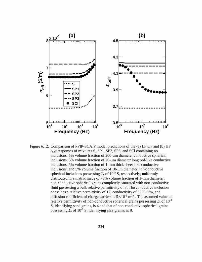
234

Figure 6.12: Comparison of PPIP-SCAIP model predictions of the (a) LF σeff and (b) HF


inclusions, 5% volume fraction of 200-μm diameter conductive spherical

inclusions, 5% volume fraction of 20-μm diameter long rod-like conductive

inclusions, 5% volume fraction of 1-mm thick sheet-like conductive

inclusions, and 5% volume fraction of 10-μm diameter non-conductive

spherical inclusions possessing Σs of 10-8 S, respectively, uniformly

distributed in a matrix made of 70% volume fraction of 1-mm diameter,

non-conductive spherical grains completely saturated with non-conductive

fluid possessing a bulk relative permittivity of 3. The conductive inclusion

phase has a relative permittivity of 12, conductivity of 5000 S/m, and

diffusion coefficient of charge carriers is 5×10-5 m2/s. The assumed value of

relative permittivity of non-conductive spherical grains possessing Σs of 10-9

S, identifying sand grains, is 4 and that of non-conductive spherical grains

possessing Σs of 10-8 S, identifying clay grains, is 8.

102

103

104

105

5

6

7

8x 10

-6

Frequency (Hz)

e

ff (

S/m

)(a)

106

107

108

3.5

3.7

3.9

4.1

4.3

4.5

Frequency (Hz)

r,

eff

(b)

S

SP1

SP2

SP3

SCl

235

Figure 6.13: Comparison of PPIP-SCAIP model predictions of the (a) LF σeff and (b) HF


inclusions, 200-μm diameter conductive spherical inclusions, 20-μm

diameter long rod-like conductive inclusions, 1-mm thick sheet-like

conductive inclusions, and 10-μm diameter non-conductive spherical grains

exhibiting Σs of 10-8 S, respectively, uniformly distributed in a matrix made

of 70% volume fraction of 1-mm diameter non-conductive spherical grains

completely saturated with electrolyte for 1% (dotted) and 2% (solid) volume

fraction of the inclusion phase. The conductive inclusion phase has a

relative permittivity of 12, conductivity of 5000 S/m, and the diffusion




grains possessing Σs of 10-9 S, identifying sand grains, is 4 and that of non-

conductive spherical grains possessing Σs of 10-8 S, identifying clay grains is

8.

102

103

104

105

0.018

0.022

0.026

0.03

0.034

Frequency (Hz)

e

ff (

S/m

)(a)

106

107

108

18

22

26

30

Frequency (Hz)

r,

eff

(b)

S

SP1

SP2

SP3

SCl

236


responses of mixtures S, SG, SP, SC, and SX containing no inclusions, 5%

volume fraction of graphite inclusions, 5% volume fraction of pyrite

inclusions, 5% volume fraction of chalcopyrite inclusions, and 5% volume

fraction of inclusions made of a synthetic low-conductivity material,

respectively, uniformly distributed in a matrix made of 70% volume fraction

of 1-mm diameter, non-conductive spherical grains that is completely

saturated with 0.1-S/m conductivity electrolyte. Pairs of Figures 14a and

14b, 14c and 14d, and 14e and 14f identify the computed σeff and εr,eff,

respectively, of mixtures containing 200-μm diameter spherical inclusions,

20-μm diameter long rod-like inclusions, and 1-mm thick sheet-like

inclusions, respectively. Relative permittivity of the electrolytic host is 80

and the diffusion coefficient of ions in the electrolyte host is 10-9 m2/s. The

assumed values of relative permittivity of non-conductive spherical grains

possessing Σs of 10-9 S, identifying sand grains, is 4. All the plots share the

same legend. Table 6.5 describes the assumed electrical properties for the

above materials.

102

103

104

105

0.015

0.02

0.025

0.03

0.035

Frequency (Hz)

e

ff (

S/m

)(a)

106

107

108

20

25

30

35

Frequency (Hz)

r,

eff

(b)

102

103

104

105

0.015

0.02

0.025

0.03

0.035

Frequency (Hz)

e

ff (

S/m

)

(c)

106

107

108

20

30

40

50

60

Frequency (Hz)

r,

eff

(d)

102

103

104

105

0

0.01

0.02

0.03

0.04

Frequency (Hz)

e

ff (

S/m

)

(e)

106

107

108

20

25

30

35

40

Frequency (Hz)

r,

eff

(f)

S

SG

SP

SC

SX

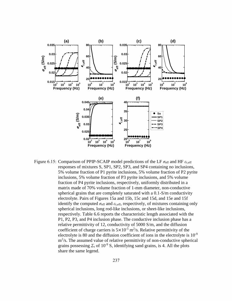
237


responses of mixtures S, SP1, SP2, SP3, and SP4 containing no inclusions,

5% volume fraction of P1 pyrite inclusions, 5% volume fraction of P2 pyrite

inclusions, 5% volume fraction of P3 pyrite inclusions, and 5% volume

fraction of P4 pyrite inclusions, respectively, uniformly distributed in a

matrix made of 70% volume fraction of 1-mm diameter, non-conductive

spherical grains that are completely saturated with a 0.1-S/m conductivity

electrolyte. Pairs of Figures 15a and 15b, 15c and 15d, and 15e and 15f

identify the computed σeff and εr,eff, respectively, of mixtures containing only

spherical inclusions, long rod-like inclusions, or sheet-like inclusions,

respectively. Table 6.6 reports the characteristic length associated with the

P1, P2, P3, and P4 inclusion phase. The conductive inclusion phase has a

relative permittivity of 12, conductivity of 5000 S/m, and the diffusion




grains possessing Σs of 10-9 S, identifying sand grains, is 4. All the plots

share the same legend.

102

103

104

105

0.015

0.02

0.025

0.03

0.035

Frequency (Hz)

e

ff (

S/m

)(a)

106

107

108

20

40

60

80

Frequency (Hz)

r,

eff

(b)

102

103

104

105

0.015

0.02

0.025

0.03

0.035

Frequency (Hz)

e

ff (

S/m

)

(c)

106

107

108

20

40

60

80

Frequency (Hz)

r,

eff

(d)

102

103

104

105

0.02

0.025

0.03

0.035

0.04

0.045

Frequency (Hz)

e

ff (

S/m

)

(e)

106

107

108

20

25

30

35

40

Frequency (Hz)

r,

eff

(f)

Sa

SP1

SP2

SP3

SP4

238

Chapter 7: Summary, Conclusions, and Recommendations

This final chapter summarizes the developments and technical contributions in the

dissertation, draws general conclusions from the results, and provides recommendations

for future research.

7.1 SUMMARY

The main thrust of this dissertation was to develop a laboratory measurement

technique and a quantitative interpretation method that explicitly account for the effects of

interfacial polarization due to conductive minerals, clay-sized particles, and clay minerals

uniformly distributed in a fluid-filled porous geological host. To do so, I developed a non-

contact and non-invasive laboratory apparatus, the WCEMIT, based on the physics of

electromagnetic induction to measure the complex electrical conductivity tensor of whole

core samples at multiple frequencies. I developed two EM forward models based on

COMSOL-based finite-element (FE) method and a MATLAB-based semi-analytic (SA)

method, respectively, of the developed tool. These EM forward models were used for

interpreting the WCEMIT measurements to estimate effective conductivity and

permittivity of the samples. Several petrophysical applications of the WCEMIT were tested

for purposes of whole core analysis of rock samples of various facies. More importantly,

the directional complex conductivity of mixtures containing conductive mineral inclusions,

such as pyrite and graphite, were estimated in the EM induction frequency range from 10

kHz to 300 kHz. Moreover, a mechanistic electrochemical model, PPIP-SCAIP model, was

developed and implemented to quantify the directional complex electrical conductivity of

mixtures containing electrically conductive mineral inclusions of various shapes uniformly

distributed in a fluid-filled, porous matrix made of non-conductive grains possessing

surface conductance. Finally, using the mechanistic model, cases of petrophysically

239

adverse alteration of subsurface galvanic resistivity, EM induction, and EM propagation

logging measurements were identified in formations containing clay particles, clay

minerals, and conductive minerals.

I successfully validated and benchmarked the new laboratory tool, the two EM

forward models of the developed tool, and the mechanistic electrochemical model against

conventional models and laboratory measurements. The WCEMIT facilitated new

measurement techniques for purposes of whole core analysis. Also, that apparatus was

utilized to measure the dielectric and frequency dispersive properties of pyrite-bearing and

graphite-bearing samples. The two EM forward models enabled conventional

petrophysical interpretation of whole core measurements and estimation of the directional

effective electrical conductivity and dielectric permittivity of pyrite-bearing and graphite-

bearing samples. The mechanistic electrochemical model allowed the simulation of

petrophysical cases for which standard electromagnetic mixing laws become invalid due

to the effects of interfacial polarization of clay particles and conductive minerals. This

simulation work emphasized situations where conventional interpretation of subsurface

galvanic resistivity, EM induction, and EM propagation logging measurements could not

provide accurate petrophysical assessments.

The second chapter of this dissertation introduced the new laboratory apparatus

capable of high-resolution multi-frequency complex conductivity tensor measurements on

whole core samples and continuous-feed cylindrical volumes in the EM induction (EMI)

frequency range of 10 kHz to 300 kHz. The apparatus is primarily a non-invasive and non-

contact measurement technique for examining whole core samples in their as-received and

re-saturated state. The COMSOL-based finite-element (FE) EM forward model and a

MATLAB-based semi-analytic (SA) EM forward model of the developed tool response

240

were validated. The semi-analytic and finite-element EM forward model predictions were

used to calibrate the complex impedance response of the nine transmitter-receiver

couplings of the WCEMIT to whole core samples.

In Chapter 3, the WCEMIT was used to measure the multi-frequency inductive-

complex electrical conductivity tensor of whole core samples of various rock facies. An

inversion scheme was invoked to processes these measurements to estimate the electrical

properties of natural and synthetic whole core samples in the EM induction frequency range

of 10 kHz to 300 kHz. The Archie’s equation, laminated sand-shale model, tensor

resistivity model, and Maxwell-Garnett effective medium model were successfully

implemented to estimate petrophysically consistent electrical properties of the whole core

samples. The effects of large dielectric permittivity, permittivity anisotropy, dielectric loss

factor, and frequency dispersive dielectric properties on the WCEMIT measurements were

simulated using the semi-analytic EM forward model. Notably, a new whole core logging

method that can improve the resistivity characterization of turbiditic and multi-layered

formations was numerically investigated using the finite-element EM forward model

coupled with a multi-layer resistivity inversion scheme.

Following that, I investigated the effects of the PPIP phenomena exhibited by

pyrite-bearing and graphite-bearing samples on their directional and frequency dispersive

electrical properties. To that end, I first used the new laboratory apparatus to measure the

directional multifrequency EM response of 4-inch-diameter, 2-feet-long glass-bead packs

containing uniformly distributed pyrite and graphite inclusions. The semi-analytic EM

forward model was then implemented to estimate the effective electrical conductivity and

dielectric permittivity of the conductive-mineral-bearing glass-bead packs. The

interpretation work in this chapter confirms that the conductive-mineral-bearing samples

241

exhibit significant frequency dispersion of electrical conductivity and dielectric

permittivity, large values of effective relative permittivity, and large alteration in the

effective conductivity due to the variations in volume content and size of conductive

mineral inclusions.

In the final part of the dissertation that includes Chapters 5 and 6, I developed a

mechanistic model to quantify the complex-valued effective electrical conductivity

response of geomaterials containing electrically conductive mineral inclusions, such as

pyrite and magnetite, uniformly distributed in a fluid-filled, porous matrix made of non-

conductive grains possessing surface conductance, such as silica grains, clay particles, and

clay-sized grains. Our model predictions are in good agreement with laboratory

measurements of multi-frequency complex-valued electrical conductivity, relaxation time,

and chargeability of mixtures containing electrically conductive inclusions. Using the

mechanistic model, I evaluated the dependence of effective complex-valued conductivity

of geological mixtures containing conductive mineral inclusions and clay particles on (a)

operating frequency, (b) conductivity of host medium, and (c) material, size, and shape of

inclusion phase. The mechanistic model predictions identified the petrophysical conditions

that give rise to significant differences of the effective conductivity and effective relative

permittivity of conductive-inclusion-bearing geomaterials from the conductivity and

relative permittivity, respectively, of the inclusion-free hydrocarbon-bearing host.

7.2 CONCLUSIONS

The conclusions are listed below according to the main objectives of this

dissertation.

242

7.2.1 Laboratory Apparatus for Multi-Frequency Inductive-Complex

Conductivity Tensor Measurements

i. The FE model predictions for the zz-coupling and yy-coupling of the WCEMIT

agreed with Maxwell-Garnett effective medium model predictions of the effective

conductivity of 1-S/m-conductivity host containing randomly distributed spherical

inclusions of conductivity in the range of 0.1 S/m to 100 S/m and radius in the range

of 0.35 inches to 0.6 inches.

ii. The real part of the induced voltage response for the zz-coupling and yy-coupling

of the WCEMIT was linearly related to the conductivity of the whole core sample

for conductivity values in the range of 0.01 S/m to 10 S/m.

iii. The computed values of geometrical factors of the zz-coupling and yy-coupling of

the WCEMIT at 58.5 kHz were similar to those obtained by Kickhofel et al. (2010)

at 51.28 kHz.

iv. The SA model predictions agreed with the FE model predictions of the zz-coupling

and yy-coupling response for various values of conductivity, dielectric permittivity,

dielectric loss factor, and operating frequencies in the range of 10 kHz to 300 kHz.

v. Tilted test loop (TTL) method was used to calibrate all the nine couplings of the

WCEMIT at seven discrete frequencies, namely 19.6, 31.2, 41.5, 58.5, 87.6, 150,

or 261 kHz.

7.2.2 Petrophysical Applications of Multi-frequency Inductive-Complex

Conductivity Tensor Measurements on Whole Core Samples

i. The SA model predictions of the WCEMIT responses of all nine transmitter-

receiver couplings to the tilted test loop were used to validate the calibrated

WCEMIT measurements.

243

ii. The calibrated WCEMIT measurements were successfully validated by comparing

the measured values with the SA model predictions of all nine transmitter-receiver

coupling responses to synthetic bi-laminar dipping whole cores oriented at any

given azimuth for various operating frequencies.

iii. Laboratory investigation corroborated the use of the WCEMIT for estimating the

true host conductivity, Archie’s porosity exponent, and formation factor of

isotropic whole cores.

iv. The WCEMIT was applied to quantify the bed conductivity, horizontal

conductivity, anisotropy ratio, dip, and azimuth of bilaminar whole core samples.

v. The WCEMIT was also used to estimate the host conductivity of vuggy whole cores

containing uniformly distributed non-conductive vugs for various volume fractions

of non-conductive vugs.

vi. Numerical investigation using the SA model confirmed that the WCEMIT response

is suitable for measuring the effects of dielectric properties, such as permittivity,

dielectric loss factor, and permittivity anisotropy, and dielectric dispersion

characteristics, denoted by the parameters of the Cole-Cole model, arising due to

the interfacial polarization phenomena.

vii. A fast inversion scheme for a newly proposed whole core logging measurement

was applied to estimate the layer-by-layer conductivity of 24-inch-long whole cores

at a vertical resolution of 1 inch and at 58.5 kHz. This method successfully

identified cemented streaks in a whole core containing randomly distributed sand,

shale, and cemented layers of minimum 1-inch thickness.

244

7.2.3 Effective Electrical Conductivity and Dielectric Permittivity of Samples

Containing Disseminated Mineral Inclusions

i. Glass-bead packs containing homogeneously dispersed pyrite and/or graphite

inclusions exhibited frequency dispersion of their R- and X-signal responses due to

the interfacial polarization of electrically conductive mineral inclusions.

ii. The R-signal response of conductive-mineral-bearing packs were significantly

different from that of the inclusion-free glass-bead packs; consequently, accurate

resistivity interpretation methods for samples containing pyrite or graphite

inclusions must account for the effects of interfacial polarization.

iii. The effective conductivity and effective relative permittivity of the conductive-

mineral-bearing glass-bead packs were successfully estimated using the SA model.

iv. The estimated values of the effective relative permittivity were in the range of 103

to 104 for the pyrite-bearing glass-bead packs, and were in the range of 104 to 106

for the graphite-bearing glass-bead packs.

v. The effective electrical conductivity and dielectric relative permittivity of the

conductive-mineral-bearing packs were strongly dependent on the operating

frequency and mineral type, volume fraction, and size of mineral inclusions.

vi. The multi-frequency effective conductivity and relative permittivity of graphite-

bearing packs were significantly different from those of the pyrite-bearing packs

due to the large difference in the diffusion coefficients of charge carriers, bulk

conductivity values, and shapes of pyrite and graphite inclusions.

vii. The packs containing homogeneously dispersed conductive inclusions exhibited

conductivity anisotropy ratio, in the range of 1 to 1.7, and permittivity anisotropy

ratio, in the range of 1.1 to 2.8. Consequently, resistivity interpretation methods for

formations containing uniformly dispersed pyrite or graphite inclusions must

245

account for the effects of effective conductivity and effective permittivity

anisotropy due to interfacial polarization of the inclusion phase.

viii. The packs containing alternating layers of different volume fraction of conductive

mineral inclusions had significantly different effective conductivity and relative

permittivity compared to those of packs containing homogeneously distributed

mineral inclusions of the same mineral type, size, total volume fraction, and shape.

ix. Accurate resistivity interpretation in formations containing conductive minerals

will require accurate knowledge of shape, size, mineral type, conductivity, and

distribution of the inclusion phase.

7.2.4 Mechanistic Model of Interfacial Polarization of Disseminated Conductive

Minerals in Absence of Redox-Active Species

i. Dipole moment of an inclusion was obtained by solving Poisson-Nernst-Planck’s

(PNP) equations of dilute solution theory. The calculated dipole moment was

coupled with a consistent Maxwell-Garnett effective-medium formulation to

determine the effective complex-valued electrical conductivity of the geomaterial

containing conductive mineral inclusions, clay particles, and clay-sized grains.

ii. The PPIP-SCAIP model was successfully validated in the frequency range from

100 Hz to 100 MHz for a characteristic length of the inclusion phase in the range

of 0.1 μm to 1 mm.

iii. The chargeability of geomaterials depend only on the volumetric content of

electrically conductive inclusions for host conductivity close to or higher than 0.01

S/m.

246

iv. The relaxation time associated with polarization of conductive spherical inclusions

was linearly related to the radius of inclusions and is inversely related to the

diffusion coefficients of charge carriers in the host and those in the inclusion phase.

v. The estimated values of diffusion coefficient of charge carriers in the electrically

conductive inclusion phase were consistent with the electrical mobility of p- and n-

charge carriers in the inclusion material.

vi. High-frequency effective conductivity increases while the low-frequency effective

conductivity decreases with an increase in the concentration of metallic inclusions

that give rise to the PPIP phenomena.

7.2.5 Effects of Disseminated Conductive Mineral Inclusions on Subsurface

Electrical Measurements

i. Electrical measurements in formations containing uniformly distributed conductive

inclusions are highly sensitive to the variations in volume fraction, material,

characteristic length, and shape of the inclusion phase and conductivity of the pore-

filling electrolyte.

ii. The low-frequency effective conductivity of a geomaterial containing as low as 5%

volume fraction of disseminated conductive inclusions was -30% to +100% more

than the host conductivity for the operating frequencies in the range of 100 Hz to

100 kHz.

iii. The high-frequency effective relative permittivity of a geomaterial containing as

low as 5% volume fraction of disseminated conductive inclusions was +90% to -

10% more than the host relative permittivity for the operating frequencies in the

range of 100 kHz to 10 MHz.

247

iv. Geomaterials containing sheet-like inclusions exhibited large frequency dispersion

of the effective conductivity in the operating frequency range of galvanic resistivity

logging tools. These geomaterials generally exhibited exceedingly large galvanic

resistivity measurements compared to the true formation resistivity.

v. EM induction and EM propagation logging measurements were less sensitive to the

variations in properties of sheet-like inclusions and highly sensitive to the variations

in properties of rod-like and spherical inclusions.

vi. Galvanic resistivity measurements were less sensitive to the variations in properties

of rod-like and spherical inclusions and highly sensitive to the variations in

properties of sheet-like inclusions.

vii. EM propagation measurements at frequencies close to and higher than 100 MHz

were not susceptible to the effects of PPIP phenomena, and could be analyzed using

a consistent the effective medium formulations.

viii. The PPIP phenomena generally led to large alteration of EM measurements, highly

dispersive complex-valued conductivity response, and high sensitivity of EM

measurements to the properties of inclusions and conductivity of pore-filling

electrolyte.

7.3 RECOMMENDATIONS FOR FUTURE WORK

The following is a list of recommendations that could advance the research topics

documented in this dissertation:

i. The WCEMIT tool operated at seven discrete frequencies. The critical frequency

associated with the frequency dispersion phenomena cannot be accurately

measured when performing discrete frequency measurements. I recommend re-

designing the transmitter resonance circuit to allow a continuous frequency

248

excitation of the transmitter coils in the EM induction frequency range. In that case,

a new method will be required for calibrating all the nine transmitter-receiver

coupling responses for the continuous frequency sweep.

ii. The WCEMIT tool operated in the frequency range of 10 kHz to 300 kHz. The

transmitter coils should be re-designed to allow a broader frequency range of

operation to accommodate the typical frequency of operation of subsurface

galvanic resistivity and EM propagation tools. In doing so, whole core

measurements using this improved apparatus can be correlated with the subsurface

galvanic resistivity and EM propagation tool measurements.

iii. A new apparatus that is designed similar to the WCEMIT but of smaller dimensions

needs to be developed to inductively measure the EM response of core plugs.

iv. The FE model generated accurate predictions of the WCEMIT response to dipping,

isotropic whole cores oriented at any azimuth angle. However, the FE model

requires close to one hour to calculate the response of one transmitter-receiver

coupling. Faster 3D finite-element EM forward model should be developed to

perform reliable inversion of the WCEMIT measurements.

v. SA model and FE model should be improved to predict the effects of variation in

magnetic permeability of whole core samples. The presence of certain mineral

inclusions leads to effective magnetic permeability of geomaterials to be more than

1.

vi. A laboratory or a numerical method is required to ascertain the range of dielectric

permittivity and dielectric loss factor of the whole core samples that can be reliably

simulated using the two EM forward models.

249

vii. Existing whole core handling procedure requires the whole cores to be slabbed at

the core laboratories before conducting any laboratory measurements. This

prevented me from obtaining full-diameter as-received whole core samples for

petrophysical investigation based on the WCEMIT. Semi-analytic and finite-

element EM forward models of the WCEMIT response to slabbed whole core

samples should be developed to facilitate WCEMIT-based core analysis in absence

of full-diameter whole core.

viii. Most of the laboratories lack methods to clean and re-saturate whole core samples.

Also, there is no method to ensure multi-phase fluid injection in a whole core to

saturate a whole core sample at different water saturations. New laboratory methods

need to be developed to overcome these limitations to extend the WCEMIT

applications to the estimation of water saturation exponent.

ix. Capabilities to perform WCEMIT measurements on whole core samples at

reservoir pressure and temperature needs to be developed.

x. Applications of the WCEMIT and the effective medium formulation developed in

Section 3.3.5 should be tested on actual whole core samples from vuggy carbonate

formations to understand the accuracy of prediction of host conductivity in the

presence of conductive/non-conductive vugs.

xi. Core-well log integration methods should be developed for layered and thinly-

laminated formations to improve the accuracy of estimates of sand resistivity and

sand fraction in such subsurface formations. To that end, the WCEMIT could

enable high resolution measurements on whole core samples for determining the

representative shale resistivity, identify cemented streaks, and quantify sand

fraction.

250

xii. Controlled WCEMIT measurements should be performed on synthetic whole core

samples made of various materials of known dielectric dispersion parameters. In

doing so, the frequency dispersion of R- and X-signal responses of the WCEMIT

to those synthetic samples can be related to the dielectric dispersion parameters of

the materials of those synthetic samples. Similarly, controlled WCEMIT

measurements should be performed on synthetic whole core samples made of

various materials of known dielectric permittivity and dielectric loss factor. In

doing so, the frequency dispersion of R- and X-signal responses of the WCEMIT

to those synthetic samples can be related to the dielectric permittivity and dielectric

loss factor of the materials of those synthetic samples

xiii. WCEMIT measurements should be performed on whole core samples from mature

shale gas formations that contain graphitic precursors due to the over-maturation of

the kerogen. In doing so, I can develop a better understanding of the relation

between kerogen maturity, electrical properties of graphitic precursors, and EM

induction multi-frequency response. Subsequently, a new resistivity interpretation

technique for subsurface EM induction measurements in mature shale gas

formations can be developed to assess the maturity of the formation and to correct

the alterations in estimation of conductivity and permittivity due to the presence of

conductive graphitic precursors.

xiv. Extensive study is required to describe and quantify the effects of salinity on the

WCEMIT response to brine-saturated conductive-mineral-bearing whole core

samples.

251

xv. Extensive study is required to describe and quantify the effects of material of the

inclusion phase on the WCEMIT response to brine-saturated conductive-mineral-

bearing whole core samples.

xvi. An inversion scheme should be coupled with the PPIP-SCAIP model to perform

joint-interpretation of subsurface galvanic resistivity, EM induction, and EM

propagation tool measurements.

xvii. PPIP-SCAIP model needs to be improved to account for the (a) randomly oriented

conductive mineral inclusions, (b) redox-active host-inclusion interfaces, (c)

ellipsoidal conductive mineral inclusions, clay particles, silica grains, and clay-

sized grains, (d) high volume fraction of conductive mineral inclusions, and (e)

multi-phase fluid distribution.

xviii. PPIP-SCAIP model should be improved to account for the (a) mutual EM

interactions between conductive mineral inclusions, clay particles, silica grains, and

clay-sized grains and (b) reduction in surface area of host-inclusion interfaces due

to the contact of neighboring grains.

xix. PPIP-SCAIP model should be improved to account for the (a) high concentration

of charge carriers in the pore-filling electrolyte, (b) percolation length of the pore

structure, (c) percolation length of the inclusion phase, (d) presence of more than

two charge carriers in the pore-filling electrolyte, (e) variation in EM field strength

with the distance from source, and (f) presence of time varying magnetic field in

the formation.

xx. PPIP-SCAIP model should be coupled with Maxwell-Wagner polarization model,

orientation polarization model, and concentration polarization model.

252

7.4 RECOMMENDATIONS FOR BEST PRACTICES

The following is a list of recommendations that needs to be adopted as best

practices:

i. Interpretation of subsurface galvanic resistivity, EM induction, and EM

propagation measurements in conductive-mineral-bearing and clay-rich formations

should always account for effects of interfacial polarization of conductive minerals,

clay particles, and clay-sized grains.

ii. Petrophysical interpretation methodology in formations susceptible to large

interfacial polarization effects should implement joint interpretation of subsurface

galvanic resistivity, EM induction, and EM propagation measurements.

iii. Existing resistivity and dielectric interpretation methods in conductive-mineral-

bearing and clay-rich formations should first estimate effective electrical properties

using the tool model, then PPIP-SCAIP-type mechanistic model should be used to

process the estimated effective electrical properties, and finally Archie-type water

saturation equations applied to obtain water saturation in the formation.

iv. Commercial laboratory apparatus capable of electrical measurements on whole

core samples should be used routinely during for purposes of improved core-well

log integration. Whole core logging of whole core samples from turbiditic and other

thinly-laminated formations should be performed for purposes of identifying

cemented streaks, obtaining electrical properties of representative shale, and

accurate assessment of sand fraction.

v. Inversion of WCEMIT-type measurements on non-dipping whole cores to obtain

effective electrical properties should be based on the semi-analytic EM forward

model instead of finite-element EM forward model.

253

Appendix A: Sheet-like inclusion in an electrolytic host

An infinite sheet of finite thickness, equal to 2a, exhibits dipolarizability along the

thickness of the sheet, while dipolarizability is negligible along its length and width. Such

an inclusion identifies a lamination or thin bed. In order to compute the dipolarizability of

the representative volume (Figure 5.3) comprising an infinite sheet-like inclusion in an

electrolytic host, equation 17 in Chapter 5 is expressed in Cartesian coordinates as

𝜕2𝑑𝑗

𝜕𝑥2= 𝛾𝑗

2𝑑𝑗, (A1)

where x is the perpendicular distance from the plane of symmetry of the sheet that divides

the sheet into two volumes of equal thickness, and j denotes the phase, such that i identifies

inclusion and h identifies host. A general solution (Morse and Feshbach, 1953) to the above

differential equation is

𝑑𝑗(𝑥) = ∑ [𝐶𝑚,𝑗e𝑛𝛾𝑗𝑥

∞

𝑚=1

+ 𝐷𝑚,𝑗e−𝑛𝛾𝑗𝑥], (A2)

where m is an integer and 𝐶𝑚,𝑗 and 𝐷𝑚,𝑗 are unknown complex-valued coefficients of the

general solution of equation A1. To simplify the analytical derivation of our model, I

assume m=1. Also, by implementing the condition that 𝑑𝑗(𝑥) should be finite at r=0 and

r= ∞, I obtain two independent particular solutions of 𝑑𝑗(𝑥) for the host, subscript h, and

inclusion, subscript i, phases that can be expressed as

𝑑𝑖(𝑥) = 2𝐶𝑖 sinh(𝛾𝑖𝑥), (A3)

and

254

𝑑ℎ(𝑥) = 𝐷ℎe−𝛾ℎ𝑥, (A4)

where 𝐶𝑖 and 𝐷ℎ are unknown complex-valued coefficients of the particular solution in the

inclusion phase and host medium, respectively, obtained from equation A2.

Assuming a separable solution for 𝜗j(x), equation 19 can now be expressed in

Cartesian coordinates as

∆𝜗𝑗 =𝜕2𝜗𝑗

𝜕𝑥2= 0. (A5)

A general solution of the above differential equation can be expressed, using m=0 for the

standing wave solution, as

𝜗𝑗(𝑥) = 𝐴0,𝑗𝑥 + 𝐵0,𝑗, (A6)

where 𝐴0,𝑗 and 𝐵0,𝑗 are unknown complex-valued coefficients of the general solution of

the differential equation A5. Now, equation A6 can be rewritten using equation 20 as

𝜑𝑗(𝑥) = 𝐴0,𝑗𝑥 + 𝐵0,𝑗 −q𝑑𝑗(𝑥)

𝛾𝑗2휀𝑗

. (A7)

The standing wave representation of equation A7 for the inclusion phase, using equation

A3, is

𝜑𝑖(𝑥) = 𝐴𝑖𝑥 −2q𝐶𝑖 sinh(𝛾𝑖𝑥)

𝛾𝑖2휀𝑖

, (A8)

where 𝐴𝑖 is an unknown complex-valued coefficient of the particular solution in the

inclusion phase obtained from equation A7. Similarly, the standing wave representation of

equation A7 for the host medium, using equation A4, is

255

𝜑ℎ(𝑥) = 𝐵ℎ −q𝐷ℎe−𝛾ℎ𝑥

𝛾ℎ2휀ℎ

, (A9)

where 𝐵ℎ is an unknown complex-valued coefficient of the particular solution in the host

obtained from equation A7.

Using boundary condition (a), equations A9 and A8 can be equated on the surface

of the sheet at x=a. I obtain the following equation:

−𝐸0𝑎 + 𝐵ℎ + 𝐸ℎ𝐷ℎ = 𝐴𝑖𝑎 + 𝐹𝑖𝐶𝑖, (A10)

where 𝐸0 is the amplitude of the externally applied electric field,

𝐸ℎ = −qe−𝛾ℎ𝑎

𝛾ℎ2휀ℎ

,

and

𝐹𝑖 = −2qsinh(𝛾𝑖𝑎)

𝛾𝑖2휀𝑖

.

The equation obtained using boundary condition (b) at the surface of the sheet can be

abbreviated as

휀ℎ(−𝐸0 + 𝐺ℎ𝐷ℎ) = 휀𝑖(𝐴𝑖 + 𝐻𝑖𝐶𝑖), (A11)

where

𝐺ℎ =qe−𝛾ℎ𝑎

𝛾ℎ휀ℎ,

and

𝐻𝑖 = −2qcosh(𝛾𝑖𝑎)

𝛾𝑖휀𝑖.

256

The equation obtained using boundary condition (c) at the outer surface of the sheet in the

host medium can be abbreviated as

𝐷ℎ = −𝜎ℎ𝐸0

i𝜔𝐺ℎ휀ℎ. (A12)

On the other hand, the equation obtained using boundary condition (c) at the inner surface

of the sheet in the inclusion medium can be abbreviated as

𝐴𝑖 = i𝜔𝐻𝑖𝐶𝑖

휀𝑖

𝜎𝑖. (A13)

When solving equations A10, A11, A12, and A13, I obtain the dipolarizability of the

representative volume comprising a sheet-like inclusion in an electrolytic host as

𝑓(𝜔) =𝐵ℎ

𝐸0𝑎= (1 −

𝐾ℎ

𝐾𝑖) +

i

𝜔𝑎[𝐾ℎ

𝐾𝑖

𝜎𝑖

휀𝑖

𝐹𝑖

𝐻𝑖−

𝜎ℎ

휀ℎ

𝐸ℎ

𝐺ℎ]. (A14)

257

Appendix B: Rod-like inclusion in an electrolytic host

A long rod of radius equal to a, such that its length ≫ a, exhibits dipolarizability

only in the radial direction, while dipolarizability is negligible in the axial direction. Such

an inclusion identifies a pore-filling mineralization. In order to compute the dipolarizability

of the representative volume (Figure 5.2) comprising a rod-like inclusion in an electrolytic

host, equation 17 in Chapter 5 can be expressed in cylindrical coordinates, assuming axial

symmetry and a separable solution for 𝑑𝑗(𝑟, 𝜃) = 𝑅𝑗(𝑟)𝑇𝑗(𝜃), as

𝑟

𝑅𝑗

𝜕𝑅𝑗

𝜕𝑟+

𝑟2

𝑅𝑗

𝜕2𝑅𝑗

𝜕𝑟2− 𝛾𝑗

2𝑟2 +1

𝑇𝑗

𝜕2𝑇𝑗

𝜕𝜃2= 0, (B1)

and

𝜕2𝑇𝑗

𝜕𝜃2= −𝑚2𝑇𝑗 , (B2)

where m is an integer for standing wave solution (Morse and Feshbach, 1953), and j denotes

the phase such that i identifies inclusion and h identifies host. A standing wave solution

(Weisstein, 2015c) to the above differential equation is

𝑇𝑗 = ∑ 𝐴𝑚,𝑗 𝑐𝑜𝑠(𝑚𝜃) + 𝐵𝑚,𝑗 𝑠𝑖𝑛(𝑚𝜃)

∞

𝑚=1

, (B3)

where 𝐴𝑚,𝑗 and 𝐵𝑚,𝑗 are unknown complex-valued coefficients of the general solution of

the differential equation B2. Using equation B2 in equation B1, I obtain

𝜕2𝑅𝑗

𝜕𝑟2+

1

𝑟

𝜕𝑅𝑗

𝜕𝑟− (

𝑚2

𝑟2+ 𝛾𝑗

2)𝑅𝑗 = 0. (B4)

258

A standing wave solution (Weisstein, 2015c) to the differential equation B4 is

𝑅𝑗 = ∑ 𝐶𝑚,𝑗I𝑚(𝑟𝛾𝑗) + 𝐷𝑚,𝑗K𝑚(𝑟𝛾𝑗)

∞

𝑚=1

, (B5)

where I𝑚 and K𝑚 are associated modified Bessel function of the first and second kind

(Weisstein, 2015c), respectively, of m-th order and 𝐶𝑚,𝑗 and 𝐷𝑚,𝑗 are unknown complex-

valued coefficients of the general solution of the differential equation B4. To simplify the

analytical derivation of our model, I assume m=1 and 𝐵𝑚,𝑗 = 0, which reduces equations

B5 and B3 to

𝑅𝑗 = 𝐶𝑗I1(𝑟𝛾𝑗) + 𝐷𝑗K1(𝑟𝛾𝑗), (B6)

and

𝑇𝑗 = 𝐴𝑗 cos(𝜃), (B7)

respectively, where 𝐶𝑗, 𝐷𝑗 , and 𝐴𝑗 and are unknown complex-valued coefficients of the

particular solution obtained from equations B3 and B5. Now, the general representation of

𝑑𝑗(𝑟, 𝜃) can be written, by combining equations B6 and B7, as

𝑑𝑗(𝑟, 𝜃) = [𝐶𝑗I1(𝑟𝛾𝑗) + 𝐷𝑗K1(𝑟𝛾𝑗)] cos(𝜃). (B8)

Using the condition that 𝑑𝑗(𝑟, 𝜃) should be finite at r=0 and r=∞, I obtain two independent

particular solutions of 𝑑𝑗(𝑥) for the host, subscript h, and inclusion, subscript i, phases that

can be represented as

𝑑𝑖(𝑟, 𝜃) = 𝐶𝑖I1(𝑟𝛾𝑖) cos(𝜃), (B9)

and

𝑑ℎ(𝑟, 𝜃) = 𝐷ℎK1(𝑟𝛾ℎ) cos(𝜃), (B10)

259

where 𝐶𝑖 and 𝐷ℎ are unknown complex-valued coefficients of the particular solution in the

inclusion phase and host medium, respectively, obtained from equation B8.

Assuming a long rod and a separable solution for 𝜗𝑗(𝑟, 𝜃, 𝑧), equation 19 can be

expressed in cylindrical coordinates as

∆𝜗𝑗 =1

𝑟

𝜕

𝜕𝑟(𝑟

𝜕𝜗𝑗

𝜕𝑟) +

1

𝑟2

𝜕2𝜗𝑗

𝜕𝜃2+

𝜕2𝜗𝑗

𝜕𝑧2= 0. (B11)

Assuming axial symmetry, a general solution (Hogg, 2001) to the above partial differential

equation can be expressed as

𝜗𝑗(𝑟, 𝜃) = 𝐴0,𝑗 + 𝐵0,𝑗 ln(𝑟) + ∑ [𝐴𝑛,𝑗𝑟𝑛 + 𝐵𝑛,𝑗𝑟−𝑛][𝐸𝑛,𝑗 cos(𝑛𝜃) + 𝐹𝑛,𝑗 sin(𝑛𝜃)]∞𝑛=1 ,

(B12)

where n is an integer and 𝐴𝑛,𝑗, 𝐵𝑛,𝑗, 𝐸𝑛,𝑗, and 𝐹𝑛,𝑗 are unknown complex-valued

coefficients of the general solution of the partial differential equation B11. For analytical

modeling purposes of our model, I assume n=1, 𝐹𝑛,𝑗 = 0, 𝐴0,𝑗 = 0, and 𝐵0,𝑗 = 0 to obtain

an alternate representation of equation B12 as

𝜗𝑗(𝑟, 𝜃) = [𝐴1,𝑗𝑟1 + 𝐵1,𝑗𝑟−1] cos(𝜃), (B13)

which can be rewritten using equation 20 as

𝜑𝑗(𝑟, 𝜃) = [𝐴1,𝑗𝑟 + 𝐵1,𝑗𝑟−1] cos(𝜃) −q𝑑𝑗(𝑟, 𝜃)

𝛾𝑗2휀𝑗

. (B14)

A standing-wave representation of equation B14 for the inclusion phase, using equation

B9, is

𝜑𝑖(𝑟, 𝜃) = 𝐴𝑖𝑟 cos(𝜃) −q𝐶𝑖I1(𝑟𝛾𝑖) cos(𝜃)

𝛾𝑖2휀𝑖

, (B15)

260

where 𝐴𝑖 is unknown complex-valued coefficient of the particular solution in the

inclusion phase obtained from equation B14. A standing-wave representation of equation

B14 for the host phase, using equation B10, is

𝜑ℎ(𝑟, 𝜃) = [−𝐸0𝑟 + 𝐵ℎ𝑟−1] cos(𝜃) −q𝐷ℎK1(𝑟𝛾ℎ) cos(𝜃)

𝛾ℎ2휀ℎ

, (B16)

where 𝐵ℎ is an unknown complex-valued coefficient of the particular solution in the host

obtained from equation B14 and 𝐸0 is the amplitude of the externally applied electric field.

Using boundary condition (a), equations B16 and B15 can be equated on the surface

of the long rod of radius equal to a. The resulting equation can be abbreviated as

−𝐸0𝑎 +𝐵ℎ

𝑎+ 𝐸ℎ𝐷ℎ = 𝐴𝑖𝑎 + 𝐹𝑖𝐶𝑖 , (B17)

where

𝐸ℎ = −qK1(𝑎𝛾ℎ)

𝛾ℎ2휀ℎ

,

and

𝐹𝑖 = −qI1(𝑎𝛾𝑖)

𝛾𝑖2휀𝑖

.

The equation obtained using boundary condition (b) at the surface of the long rod can be

abbreviated as

휀ℎ(𝐸0 +𝐵ℎ

𝑎2+ 𝐺ℎ𝐷ℎ) = 휀𝑖(𝐴𝑖 + 𝐻𝑖𝐶𝑖), (B18)

where

𝐺ℎ = −q

𝛾ℎ휀ℎ[−K0(𝑎𝛾ℎ) −

K1(𝑎𝛾ℎ)

𝛾ℎ𝑎],

261

and

𝐻𝑖 = −q

𝛾𝑖휀𝑖[I0(𝑎𝛾𝑖) −

I1(𝑎𝛾𝑖)

𝛾𝑖𝑎].

On the other hand, the equation obtained using boundary condition (c) at the outer surface

of the long rod in the host medium can be abbreviated as

𝐵ℎ = −𝑎2 (𝐸0 + i𝜔𝐺ℎ𝐷ℎ

휀ℎ

𝜎ℎ). (B19)

The equation obtained using equation boundary condition (c) at the inner surface of the rod

in the inclusion medium can be abbreviated as

𝐴𝑖 = i𝜔𝐻𝑖𝐶𝑖

휀𝑖

𝜎𝑖. (B20)

When solving equations B17, B18, B19, and B20, I obtain the dipolarizability of the

representative volume comprising a rod-like inclusion in an electrolytic host as

𝑓(𝜔) =𝐵ℎ

𝐸0𝑎2= −1 +

2i𝜔

[1𝑎

𝐾ℎ

𝐾𝑖

𝜎𝑖

휀𝑖

𝐹𝑖

𝐻𝑖−

1𝑎

𝜎ℎ

휀ℎ

𝐸ℎ

𝐺ℎ+ i𝜔 (

𝐾ℎ

𝐾𝑖+ 1)]

. (B21)

262

Appendix C: Spherical inclusion in an electrolytic host

A sphere of radius equal to a exhibits dipolarizability in the radial direction. Such

an inclusion identifies a grain or vug. In order to compute the dipolarizability of the

representative volume (Figure 5.2) comprising a spherical inclusion in an electrolytic host,

equation 17 in Chapter 5 can be expressed in spherical coordinates, assuming azimuthal

symmetry, axial symmetry, and a separable solution (Young, 2009) for 𝑑𝑗(𝑟, 𝜃) =

𝑅𝑗(𝑟)𝑇𝑗(𝜃) as

1

𝑅𝑗

𝜕

𝜕𝑟(𝑟2

𝜕𝑅𝑗

𝜕𝑟) − 𝛾𝑗

2𝑟2 +1

𝑇𝑗 sin(𝜃)

𝜕

𝜕𝜃(sin(𝜃) 𝜕𝑇𝑗

𝜕𝜃) = 0, (C1)

and

1

sin(𝜃)

𝜕

𝜕𝜃(

sin(𝜃) 𝜕𝑇𝑗

𝜕𝜃) = −𝑛(𝑛 + 1)𝑇𝑗 , (C2)

where n is an integer for the standing wave solution, and j denotes the phase such that i

identifies inclusion and h identifies host. A standing-wave solution (Young, 2009) to the

above differential equation is

𝑇𝑗 = ∑ 𝐴𝑛,𝑗P𝑛0(cos(𝜃)) + 𝐵𝑛,𝑗

∞

𝑛=1

Q𝑛0 (cos(𝜃)), (C3)

where P𝑛0 and Q𝑛

0 are associated Legendre functions of the first and second kind (Weisstein,

2015a), respectively, of n-th order and 𝐴𝑛,𝑗 and 𝐵𝑛,𝑗 are unknown complex-valued

coefficients of the general solution of the partial differential equation C2. Using equation

C2 in equation C1, I obtain

263

𝜕

𝜕𝑟(𝑟2

𝜕𝑅𝑗

𝜕𝑟) − [𝛾𝑗

2𝑟2 + 𝑛(𝑛 + 1)]𝑅𝑗 = 0. (𝐶4)

A standing-wave solution to the above differential equation is

𝑅𝑗 = ∑ 𝐶𝑛,𝑗i𝑛(𝑟𝛾𝑗) + 𝐷𝑛,𝑗k𝑛(𝑟𝛾𝑗)

∞

𝑛=1

, (C5)

where n is an integer for the standing-wave solution (Young, 2009), i𝑛 and k𝑛 are the

modified spherical Bessel function of the first and second kind (Weisstein, 2015b),

respectively, of n-th order and 𝐶𝑛,𝑗 and 𝐷𝑛,𝑗 are unknown complex-valued coefficients of

the general solution of the partial differential equation C4; 𝑖𝑛 and 𝑘𝑛 can be expressed in

terms of modified Bessel function of the first and second kind, respectively, as

𝑖𝑛(𝑟𝛾𝑗) = √π

2𝑟𝛾𝑗I

𝑛+12

(𝑟𝛾𝑗),

and

𝑘𝑛(𝑟𝛾𝑗) = √2

π𝑟𝛾𝑗K

𝑛+12

(𝑟𝛾𝑗),

where I𝑛+

1

2

and K𝑛+

1

2

are the modified Bessel function of the first and second kind,

respectively, of n-th order. To simplify the analytical derivation of our model, I reduce the

series to a single term and use n=1 and 𝐵𝑛,𝑗 = 0 by taking into account the following

symmetries of the charge density: (1) axial symmetry, (2) anti-symmetry with respect to 𝜃,

and (3) dipolar nature of the externally applied field. This reduces equations C5 and C3 to

264

𝑅𝑗 = [𝐶𝑗√𝜋

2𝑟𝛾𝑗𝐼3

2(𝑟𝛾𝑗) + 𝐷𝑗√

2

𝜋𝑟𝛾𝑗𝐾3

2(𝑟𝛾𝑗)], (C6)

and

𝑇𝑗 = 𝐴𝑗 cos(𝜃), (C7)

respectively, where 𝐶𝑗, 𝐷𝑗 , and 𝐴𝑗 and are unknown complex-valued coefficients of the

particular solution obtained from equations C3 and C5. The general representation of

𝑑𝑗(𝑟, 𝜃) can now be written, by combining equations C6 and C7, as

𝑑𝑗(𝑟, 𝜃) = [𝐶𝑗𝑖1(𝑖𝑟𝛾𝑗) + 𝐷𝑗𝑘1(𝑖𝑟𝛾𝑗)] cos(𝜃). (C8)

Using the condition that 𝑑𝑗(𝑟, 𝜃) should be finite at r=0 and r=∞, I obtain two independent

particular solutions of 𝑑𝑗(𝑥) for the host, subscript h, and inclusion, subscript i, phases that

can be represented as

𝑑𝑖(𝑟, 𝜃) = 𝐵𝑖i1(𝑟𝛾𝑖) cos(𝜃),

or

𝑑𝑖(𝑟, 𝜃) = 𝐵𝑖[cosh(𝑟𝛾𝑖)

𝑟𝛾𝑖−

sinh(𝑟𝛾𝑖)

𝑟𝛾𝑖] cos(𝜃), (C9)

and

𝑑ℎ(𝑟, 𝜃) = 𝐵ℎk1(𝑟𝛾ℎ) cos(𝜃),

or

𝑑ℎ(𝑟, 𝜃) = 𝐵ℎ[e−𝑟𝛾ℎ (1

𝑟𝛾ℎ+

1

(𝑟𝛾ℎ)2)] cos(𝜃), (C10)

where 𝐵𝑖 and 𝐵ℎ are unknown complex-valued coefficients of the particular solution in the

inclusion phase and host medium, respectively, obtained from equation C8.

265

Assuming azimuthal symmetry and a separable solution for 𝜗𝑗(𝑟, 𝜃, 𝜑) =

𝑅𝜖𝑗(𝑟)𝑇𝜖𝑗(𝜃), equation 19 can be expressed in spherical coordinates as

∆𝜗𝑗 =1

𝑅𝜖𝑗

𝜕

𝜕𝑟(𝑟2

𝜕𝑅𝜖𝑗

𝜕𝑟) +

1

𝑇𝜖𝑗 sin(𝜃)

𝜕

𝜕𝜃(sin(𝜃) 𝜕𝑇𝜖𝑗

𝜕𝜃) = 0. (C11)

Assuming axial symmetry, a general solution (Hogg, 2001) to the above partial differential

equation can be expressed as

𝜗𝑗(𝑟, 𝜃) = ∑[𝐴𝑛,𝑗𝑟𝑛 + 𝐵𝑛,𝑗𝑟−(𝑛+1)][𝐸𝑛,𝑗 P𝑛0(cos(𝑛𝜃)) + 𝐹𝑛,𝑗Q𝑛

0 (sin(𝑛𝜃))]

∞

𝑛=0

, (C12)

where n is an integer and 𝐴𝑛,𝑗, 𝐵𝑛,𝑗, 𝐸𝑛,𝑗, and 𝐹𝑛,𝑗 are unknown complex-valued

coefficients of the general solution of the partial differential equation C11. For analytical

modeling purposes for our model, I assume n=1, 𝐹𝑛,𝑗 = 0, 𝐴0,𝑗 = 0, and 𝐶0,𝑗 = 0, as these

terms do not satisfy the polar angle dependence of the model, to obtain an alternate

representation of equation C12 as

𝜗𝑗(𝑟, 𝜃) = [𝐴1,𝑗𝑟1 + 𝐶1,𝑗𝑟−2] cos(𝜃),

which can be rewritten using equation 20 as

𝜑𝑗(𝑟, 𝜃) = [𝐴1,𝑗𝑟 + 𝐶1,𝑗𝑟−2] cos(𝜃) −q𝑑𝑗(𝑟, 𝜃)

𝛾𝑗2휀𝑗

. (C13)

A standing-wave representation of equation C13 for the inclusion phase, using C9, is

𝜑𝑖(𝑟, 𝜃) = 𝐴𝑖𝑟 cos(𝜃) −q𝐵𝑖

𝛾𝑖2휀𝑖

[cosh(𝑟𝛾𝑖)

𝑟𝛾𝑖−

sinh(𝑟𝛾𝑖)

𝑟𝛾𝑖] cos(𝜃), (C14)

266

where 𝐴𝑖 is unknown complex-valued coefficient of the particular solution in the inclusion

phase obtained from equation C13. A standing-wave representation of equation C13 for

the host phase, using C10, is

𝜑ℎ(𝑟, 𝜃) = [−𝐸0𝑟 + 𝐶ℎ𝑟−2] cos(𝜃) −q𝐵ℎ

𝛾ℎ2휀ℎ

[e−𝑟𝛾ℎ (1

𝑟𝛾ℎ+

1

(𝑟𝛾ℎ)2)] cos(𝜃), (C15)

where 𝐶ℎ is unknown complex-valued coefficient of the particular solution in the host

obtained from equation C13 and 𝐸0 is the amplitude of the externally applied electric field.

Using boundary condition (a), equations C14 and C15 can be equated on the surface

of the sphere of radius equal to a. The resulting equation can be abbreviated as

−𝐸0𝑎 +𝐶ℎ

𝑎2− 𝐸ℎ𝐵ℎ = 𝐴𝑖𝑎 − 𝐹𝑖𝐵𝑖, (C16)

where

𝐸ℎ =q

𝛾ℎ2휀ℎ

[e−𝑎𝛾ℎ (1

𝑎𝛾ℎ+

1

(𝑎𝛾ℎ)2)],

and

𝐹𝑖 =q

𝛾𝑖2휀𝑖

[cosh(𝑎𝛾𝑖)

𝑎𝛾𝑖−

sinh(𝑎𝛾𝑖)

𝑎𝛾𝑖].

The equation obtained using boundary condition (b) at the surface of the sphere can be

abbreviated as

휀ℎ(−𝐸0 −2𝐶ℎ

𝑎3+ 𝐺ℎ𝐵ℎ) = 휀𝑖(𝐴𝑖 + 𝐻𝑖𝐵𝑖), (C17)

where

𝐺ℎ =q

𝛾ℎ휀ℎe−𝑎𝛾ℎ [

1

𝑎𝛾ℎ+

2

(𝑎𝛾ℎ)2+

2

(𝑎𝛾ℎ)3],

267

and

𝐻𝑖 =𝑞

𝛾𝑖휀𝑖[2 cosh(𝑎𝛾𝑖)

(𝑎𝛾𝑖)2−

sinh(𝑎𝛾𝑖)

𝑎𝛾𝑖−

2sinh(𝑎𝛾𝑖)

(𝑎𝛾𝑖)3].

Similarly, the equation obtained using boundary condition (c) at the outer surface of the

sphere in the host medium can be abbreviated as

𝐶ℎ = −𝑎3(𝐸0

2+

i𝜔𝐺ℎ𝐵ℎ

2𝜎ℎ). (C18)

On the other hand, the equation obtained using boundary condition (c) at the inner surface

of the sphere in the inclusion medium can be abbreviated as

𝐴𝑖 =i𝜔𝐻𝑖𝐵𝑖

𝜎𝑖. (C19)

When solving equations C16, C17, C18, and C19, I obtain the dipolarizability of the

representative volume comprising a spherical inclusion in an electrolytic host as

𝐶ℎ

𝐸0𝑎3= −

1

2+

3

2

i𝜔

[2𝑎

𝜎ℎ

휀ℎ

𝐸ℎ

𝐺ℎ−

2𝑎

𝐾ℎ

𝐾𝑖

𝜎𝑖

휀𝑖

𝐹𝑖

𝐻𝑖+ i𝜔 (

2𝐾ℎ

𝐾𝑖+ 1)]

. (C20)

268

Symbols and Nomenclature

i = √−1

T = Absolute temperature (K)

휀0 = Absolute permittivity (F/m)

E0 = Amplitude of externally applied electric field (V/m)

ω = Angular frequency of externally applied electric field (rad/s)

λ = Anisotropy ratio

Σ = Apparent complex conductivity (S/m)

m = Archie’s porosity exponent

P𝑚0 = Associated Legendre function of first kind of m-th order

Q𝑚0 = Associated Legendre function of first kind of m-th order

β = Azimuth angle (°)

kB = Boltzmann’s constant (J/K)

C = Chalcopyrite

a = Characteristic length of inclusion phase (m)

N = Charge-carrier density (charge-carriers/m3)

Z = Charge number of charge carrier

K = Complex electrical conductivity (S/m)

Σ = Complex electrical conductivity tensor (S/m)

E = Complex representation of externally applied electric field (V/m)

I = Current (A)

𝜆D = Debye screening length (m)

L = Depolarization factor of inclusion phase

ε = Dielectric permittivity (F/m)

269

d = Difference of variation in positive charge-carrier density and that in

negative

charge-carrier density (charge-carriers/m3)

D = Diffusion coefficient of charge carriers (m2/s)

θ = Dip angle (°)

f = Dipolarizability or dipole coefficient of an inclusion

x = Distance between two objects (m)

r = Distance along normal to interface (m)

q = Elementary charge (C)

σ = Electrical conductivity (S/m)

I = Electrical current (A)

µ = Electrical mobility (m2/(V.s))

e = Electric field (V/m)

φ = Electric potential (V)

EM = Electromagnetic

EMI = Electromagnetic Induction

e = Euler’s number

FE = Finite element

G = Geometrical factor of a transmitter-receiver coupling (m.Ω/s)

∇ = Gradient operator

HF = High Frequency

X = Imaginary part of the apparent complex conductivity

v = Induced voltage (V)

∆ = Laplace operator

270

= Lichtenecker-Rother’s geometrical arrangement factor

LF = Low Frequency

b = Magnetic field (T)

μ = Magnetic permeability (H/m)

Cl = Mixture containing dispersed clays

G = Mixture containing graphite

P = Mixture containing pyrite

SCl = Mixture containing sand and dispersed clays

SP = Mixture containing sand and pyrite

Im = Modified Bessel function of first kind of m-th order

Km = Modified Bessel function of second kind of m-th order

im = Modified spherical Bessel function of first kind of m-th order

km = Modified spherical Bessel function of second kind of m-th order

P = Net charge (C)

PP = Perfectly polarized

PPIP = Perfectly polarized interfacial polarization

Θ = Phase angle (°)

a’ = Radius of transmitter and receiver coils (m)

εr = Relative dielectric permittivity

R = Real part of the apparent complex conductivity

SA = Semi analytic

n = Shape factor of inclusion phase

δ = Skin depth (m)

Σs = Surface conductance (S)

271

SCAIP = Surface-conductance-assisted interfacial polarization

s = Sum of variation in positive charge-carrier density and that in negative

charge-carrier density (charge-carriers/m3)

t = Time (s)

Z = Transimpedance of a transmitter-receiver coupling (V/A)

TR = Transmitter-receiver

c = Variation in charge-carrier density (charge-carriers/m3)

ϕ = Volume fraction (v/v)

k = Wavenumber (m-1)

Subscripts

app = Apparent

0 = At time equal to 0 seconds

B = Bucking

c = Conductivity

eff = Effective

p = Permittivity

f = Free

hor = Horizontal

h = Host medium

i = Inclusion phase

g = Indices for orthogonal coils in the transmitter coil system

k = Indices for orthogonal coils in the receiver coil system

r = Relative

272

R = Receiver

s = static

tot = Total

T = Transmitter

t = True

gk = Transmitter-receiver coupling

j = Type of medium/phase, either host (h) or inclusion (i)

�̂� = Unit vector

vert = Vertical

w = Water

Superscripts

- = Negatively charged carrier

+ = Positively charged carrier

* = Complex-valued

273

References

Abdel Aal, G. Z., E. A. Atekwana, and A. Revil, 2014, Geophysical signatures of

disseminated iron minerals: A proxy for understanding subsurface

biophysicochemical processes: Journal of Geophysical Research –

Biogeosciences, 119(9), 1831-1849.

Achour, M. E., M. E. Malhi, J. L. Miane, F. Carmona, and F. Lahjomri, 1999, Microwave

properties of carbon black-epoxy resin composites and their simulation by means of

mixture laws: Journal of Applied Polymer Science, 73, 969-973.

Al Duba, 1983, Electrical conductivity of Colorado oil shale to 900 °C: Fuel, 62(8), 966-

972.

Al Duhailan, M. A. and S. Cumella, 2014, Niobrara maturity goes up, resistivity goes

down; what’s going on?: Presented at the Unconventional Resources Technology

Conference.

Allan, A. M., T. Vanorio, and J. E. Dahl, 2013, Thermal maturation-induced variation of

P-wave anisotropy and dry resistivity of organic-rich shale: Presented at the Annual

Meeting, SEG.

Altman, R., B. Anderson, J. Rasmus, and M. G. Lüling, 2008, Dielectric effects and

resistivity dispersion on induction and propagation-resistivity logs in complex

volcanic lithologies: A case study: Presented at the 49th Annual Logging Symposium,

SPWLA.

Anderson, B. I., T. D. Barber, and T. M. Habashy, 2002, Interpretation and inversion of

fully triaxial induction data – a sensitivity study: Presented at the 43rd Annual Logging

Symposium, SPWLA.

274

Anderson, B., T. Barber, and M. Lüling, 2006, Observations of large dielectric effects on

induction logs, or can source rocks be detected with induction measurements:

Presented at the 47th Annual Logging Symposium, SPWLA.

Anderson, B., T.D. Barber, M. Lüling, J. Rasmus, P.N. Sen, J.R. Tabanou, and M.

Haugland, 2007, Observations of large dielectric effects on LWD propagation-

resistivity logs: Presented at the 48th Annual Logging Symposium, SPWLA.

Anderson, B., T. Barber, M. Lüling, P. Sen, R. Taherian, and J. Klein, 2008, Identifying

potential gas-producing shales from large dielectric permittivities measured by

induction quadrature signals: Presented at the 49th Annual Logging Symposium,

SPWLA.

Arroyo F. J., F. Carrique, T. Bellini, and A. V. Delgado, 1999, Dielectric dispersion of

colloidal suspensions in the presence of Stern Layer conductance – Particle size

effects: Journal of Colloid and Interface Science, 210(1), 194-199.

Asami, K., E. Gheorghiu, and T. Yonezawa, 1999, Real-time monitoring of yeast cell

division by dielectric spectroscopy: Biophysical Journal, 76, 3345-3348.

Barber, T., 1987, Spatial frequency method and apparatus for investigating earth

conductivity with high vertical resolution by induction techniques: U. S. Patent

4,837,517.

Beltramo, P. J. and E. M. Furst, 2012, Dielectric spectroscopy of bidisperse colloidal

suspensions: Journal of Colloid and Interface Science, 380(1), 34-41.

Bergosh, J. L., T. R. Marks, and A. F. Mitkus, 1985, New core analysis techniques for

naturally fractured reservoirs: Presented at the California Regional Meeting, SPE.

Buseck, P. R. and O. Beyssac, 2014, From organic matter to graphite – Graphitization:

Elements, 10(6), 421-426.

275

Chen, H. and Z. Heidari, 2014, Pore-scale evaluation of dielectric measurements in

formations with complex pore and grain structures: Presented at the 55th Annual

Logging Symposium, SPWLA.

Chu, K. T. and M. Z. Bazant, 2006, Nonlinear electrochemical relaxation around

conductors: Physical Review E, 74(1), 011501.

Clavier, C., A. Heim, and C. Scala, 1976, Effect of pyrite on resistivity and other logging

measurements: Presented at the 17th Annual Logging Symposium, SPWLA.

Clennell, M. B., M. Josh, L. Esteban, C. D. Piane, S. Schmid, M. Verrall, and B. McMullan,

2010, The influence of pyrite on rock electrical properties – A case study from NW

Australian gas reservoirs: Presented at the 51st Annual Logging Symposium, SPWLA.

Corley, B., A. Garcia, H. M. Maurer, M. B. Rabinovich, Z. Zhou, P. DuBois, and N. Shaw,

2010, Study of unusual responses from multiple resistivity tools in the Bossier

formation of the Haynesville shale play: Presented at the Annual Technical

Conference and Exhibition, SPE.

Cosenza, P., A. Ghorbani, C. Camerlynck, F. Rejiba, R. Guérin, and A. Tabbagh, 2009,

Effective medium theories for modeling the relationships between electromagnetic

properties and hydrological variables in geomaterials: Near Surface Geophysics, 7(5),

563-578.

de Kuijper, A. and J. A. de Waal, 2007, An effective-medium saturation model for

carbonate rock: Presented at the Middle East Regional Symposium. SPWLA.

Delgado, A. V., F. J. Arroyo, F. González-Caballero, V.N. Shilov, and Y.B. Borkovskaya,

1998, The effect of the concentration of dispersed particles on the mechanisms of low-

frequency dielectric dispersion (LFDD) in colloidal suspensions: Colloids and

Surfaces A: Physicochemical and Engineering Aspects, 140(1), 139-149.

276

Dias, C. A., 2000, Developments in a model to describe low-frequency electrical

polarization of rocks: Geophysics, 65(2), 437-451.

Doll, H. G., 1949, Introduction to induction logging and application to logging of wells

drilled with oil base mud: Journal of Petroleum Technology, 1(6), 148-162.

Dukhin, S. S., V. N. Shilov, and J. J. Bikerman, 1974, Dielectric phenomena and double

layer in disperse systems and polyelectrolytes: Journal of The Electrochemical

Society, 121(4), 154C.

Ehrenberg, S. N., 2007, Whole core versus plugs – scale dependence of porosity and

permeability measurements in platform carbonates: AAPG Bulletin, 91(6), 835-846.

Franklin Miller Inc., 2015, Material bulk densities, https://www.franklinmiller.com/latest-

news/material-bulk-densities/, accessed 11 July 2015.

Gander, W., and W. Gautschi, 2000, Adaptive quadrature – revisited: BIT Numerical

Mathematics, 40(1), 84-101.

Garcia-Martin, J., J. Gomez-Gil, and E. Vazquez-Sanchez, 2011, Non-destructive

techniques based on eddy current testing: Sensors, 11(3), 2525-2565.

Garrouch, A. A., 1998, Implications of resistivity dispersion on LWD log interpretations:

Presented at the SPWLA 39th Annual Logging Symposium.

Ghorbani, A., C. Camerlynck, N. Florsch, P. Cosenza, and A. Revil, 2007, Bayesian

inference of the Cole-Cole parameters from time- and frequency-domain induced

polarization: Geophysical Prospecting, 55(4), 589-605.

Gianzero, S., 1999, The paradox of anisotropy revisited: The Log Analyst, 40(6), 485-491.

Giordano, S., 2003, Effective medium theory for dispersions of dielectric

ellipsoids: Journal of Electrostatics, 58(1), 59-76.

277

Gray, T. and J. C. Rasmus, 1988, A laboratory study of oomoldic rock substantiating a

conductivity-dielectric interpretation technique and the non-interdependence of the

Archie petrophysical parameter: Presented at the 29th Annual Logging Symposium,

SPWLA.

Grosse, C. and K. R. Foster, 1987, Permittivity of a suspension of charged spherical

particles in electrolyte solution: Journal of Physical Chemistry, 91(11), 3073-3076.

Grosse, C., 1988, Permittivity of a suspension of charged spherical particles in electrolyte

solution, Part 2 – Influence of the surface conductivity and asymmetry of the

electrolyte on the low- and high-frequency relaxations: The Journal of Physical

Chemistry, 92(13), 3905-3910.

Grosse, C., 1989, Permittivity of a suspension of charged cylindrical particles in electrolyte

solution: The Journal of Physical Chemistry, 93(15), 5865-5869.

Grosse, C. and R. Barchini, 1992, The influence of diffusion on the dielectric properties of

suspensions of conductive spherical particles in an electrolyte: Journal of Physics D,

25(3), 508-515.

Grote, M. J., 1998, Nonreflecting boundary conditions for electromagnetic scattering:

Research Report No. 98-09, Seminar für Angewandte Mathematik.

Gurin, G., K. Titov, Y. Ilyin, and A. Tarasov, 2015, Induced polarization of disseminated

electronically conductive minerals: a semi-empirical model: Geophysics Journal

International, 200, 1555-1565.

Han, M., J. Cuadros, C. A. P. Suarez, E. Decoster, O. Faivre, L. Mosse, and N. Seleznev,

2012, Continuous estimate of cation exchange capacity from log data – a new

approach based on dielectric dispersion analysis: Presented at the 53rd Annual Logging

Symposium, SPWLA.

278

Hanai, T., N. Koizumi, and R. Gotoh, 1959, Dielectric properties of emulsions: Kolloid-

Zeitschrift, 167(1), 41-43.

Hanai, T., K. Asami, and N. Koizumi, 1979, Dielectric theory of concentrated suspensions

of shell-spheres in particular reference to the analysis of biological cell

suspensions: Bulletin of the Institute of Chemical Research, Kyoto University, 57,

297-305.

Hizem, M., H. Budan, B. Deville, O. Faivre, L. Mosse, and M. Simon, 2008, Dielectric

dispersion – A new wireline petrophysical measurement: Presented at the Annual

Technical Conference and Exhibition, SPE.

Hogg,A.J., 2001, Separable solutions to Laplace’s equation,

http://www.maths.bris.ac.uk/~maajh/fluids/handout3.pdf, accessed 11 June 2015.

Homan, D., J. W. Gibson, J. Jalfin, H. Wang, C. Dupius, and G. N. Minerbo, 2009, Method

of and apparatus for measuring tensor resistivity: Provisional Patent Appl.

CA2646843 A1.

Honarpour, M. M., N. F. Djabbarah, and K. Sampath, 2003, Whole core analysis –

experience and challenges: Presented at the 13th Middle East Oil Show and

Conference, SPE.

Jackson, C. and T. Hagiwara, 1998, A new simultaneous anisotropy and dielectric

correction algorithm for LWD resistivity measurements: Presented at the 39th Annual


Jackson, P. D., M. A. Lovell, J. Roberts, P. Schultheiss, D. Gunn, R. Flint, A. Wood, and

R. Holmes, 2006, Rapid non-contacting resistivity logging of core: Presented at the

45th Annual Logging Symposium, SPWLA.

279

Jackson, P. D., J. F. Williams, L. Ma, A. Camps, C. Rochelle, and A. E. Mildowski, 2008,

An investigation of the exponent in Archie’s equation: Presented at the 49th Annual


Jiangqing, Z., Z. Ding, L. Xuewen, C. Ruihua, and Y. Chunsheng, 1994, Laboratory

measurement and applications of anisotropy parameters of rock: Presented at the

SPWLA 35th Annual Logging Symposium.

Josh, M., L. Esteban, C. Delle Piane, J. Sarout, D. N. Dewhurst, and M. B. Clennell, 2012,

Laboratory characterization of shale properties: Journal of Petroleum Science and

Engineering, 88, 107-124.

Josh, M., 2014, Dielectric Permittivity – A Petrophysical Parameter for Shales:

Petrophysics, 55(04), 319-332.

Josh, M. and B. Clennell, 2015, Broadband electrical properties of clays and shales –

Comparative investigations of remolded and preserved samples: Geophysics, 80,

D129-D143.

Jougnot, D., A. Ghorbani, A. Revil, P. Leroy, and P. Cosenza, 2010, Spectral induced

polarization of partially saturated clay-rocks: a mechanistic approach: Geophysical

Journal International, 180, 210-224.

Keelan, D. K., 1982, Core analysis for aid in reservoir description: Journal of Petroleum

Technology, 34(11), 2483-2491.

Ken, A. and M. Stewart, 1999, Surface production operations – Design of gas-handling

systems and facilities, Vol. 2, Gulf Professional Publishing.

Kennedy, M. W., S. Akhtar, J. A. Bakken, and R. E., Aune, 2011, Analytical and

experimental validation of electromagnetic simulations using COMSOL re-

280

inductance, induction heating, and magnetic fields: Presented at the COMSOL Users

Conference.

Kennedy, W. D. and D. C. Herrick, 2004, Conductivity anisotropy in shale-free sandstone:

Petrophysics, 45(1), 38-58.

Kethireddy, N., H. Chen, and Z. Heidari, 2014, Quantifying the effect of kerogen on

resistivity measurements in organic-rich mudrocks: Petrophysics, 55(2), 136-146.

Khair, A. S. and T. M. Squires, 2008, Fundamental aspects of concentration polarization

arising from nonuniform electrokinetic transport: Physics of Fluids, 20, 087102.

Kickhofel, J. L., A. Mohamide, J. Jalfin, J. Gibson, P. Thomas, G. Minerbo, and D. M.

Homan, 2010, Inductive conductivity tensor measurement for flowline or material

samples: Review of Scientific Instruments, 81(7), 075102.

Kilic, D. S., 2014, Tilted test loop calibration system: Provisional Patent Appl.

US20140156211 A1.

Klein, J. D. and W. R. Sill, 1982, Electrical properties of artificial clay-bearing sandstone:

Geophysics, 47(11), 1593-1605.

Klein, J. D., 1996, Saturation effects on electrical anisotropy: The Log Analyst, 37(1), 47-

49.

Klein, J. D., P. R. Martin, and D. Allen, The petrophysics of electrically anisotropic

reservoirs: The Log Analyst, 38(3), 25-36.

Kriegshäuser, B., O. Fanini, S. Forgang, G. Itskovich, M. Rabinovich, L. Tabarovsky, L.

Yu, M. Epov, and J. van-der-Horst, 2000, A new multi-component induction logging

tool to resolve anisotropic formations: Presented at the 41st Annual Logging

Symposium, SPWLA.

Laswell, P. M., 2006, Core analysis for electrical properties: Petrophysics, 47(3), 191-213.

281

Laughrey, C. D., T. E. Ruble, H. Lemmens, J. Kostelnik, A. R. Butcher, G. Walker, and

W. Knowles, 2011, AV black shale diagenesis – insights from integrated high-

definition analyses of post-mature Marcellus formation rocks, Northeastern

Pennsylvania: Presented at the Annual Convention and Exhibition, AAPG.

Le, F., Z. Zhou, H. Maurer, and M. Rabinovich, 2011, 3-D study of resistivity tool

responses in formations with vertical fractures or horizontal transverse isotropy:

Presented at the 52nd Annual Logging Symposium, SPWLA.

Leao, T. P., E. Perfect, and J. S. Tyner, 2015, Evaluation of Lichtenecker’s mixing model

for predicting effective permittivity of soils at 50 MHz: Transactions of the ASABE,

58(1), 83-91.

Lee, S., 2010, Development of approach to estimate volume fraction of multiphase material

using dielectrics: Ph.D. dissertation, Texas A&M University.

Leroy, P. and A. Revil, 2004, A triple layer model of the surface electrochemical properties

of clay minerals: Journal of Colloid and Interface Science, 270(2), 371-380.

Lesmes, D. P. and F. D. Morgan, 2001, Dielectric spectroscopy of sedimentary rocks:

Journal of Geophysical Research, 106(B7), 13329-13346.

Loftness, R. L., 1952, The dielectric losses of various filled phenolic resins: Ph.D.

dissertation, ETH Zurich.

Lüling, M. G., L. Pettinicchio, R. A. Rosthal, and F. Shray, 2005, Dielectric effects on

resistivity anisotropy in laminates: Presented at the 46th Annual Logging Symposium,

SPWLA.

Luo, Y. and G. Zhang, 1998, Theory and application of spectral induced polarization:

Society of Exploration Geophysicists.

282

Mahan, M. K., J. D. Redman, and D. W. Strangway, 1986, Complex resistivity of synthetic

sulphide bearing rocks: Geophysical Prospecting, 34(5), 743-768.

Misra, S., C. Torres-Verdín, and K. Sepehrnoori, 2013, Environmental and transport effects

on core measurements of water saturation, salinity, and wettability: Presented at the

Annual Technical Conference and Exhibition, SPE.

Misra, S., C. Torres-Verdín, D. Homan, and J. Rasmus, 2015a, Complex electrical

conductivity of mudrocks and source-rock formations containing disseminated

pyrite: Presented at the Unconventional Resources Technology Conference, SPE-

AAPG-SEG.

Misra, S., C. Torres-Verdín, D. Homan, G. Minerbo, and J. Rasmus, 2015b, Laboratory

investigation of petrophysical applications of multi-frequency inductive-complex

conductivity tensor measurements: Presented at the 56th Annual Logging Symposium,

SPWLA.

Misra, S., C. Torres-Verdín, A. Revil, D. Homan, and J. Rasmus, 2015c, Interfacial

polarization of disseminated conductive minerals in absence of redox-active species,

Part 1 – Mechanistic model and validation: Intended for publication in Geophysics

Journal.

Misra, S., C. Torres-Verdín, A. Revil, D. Homan, and J. Rasmus, 2015d, Interfacial

polarization of disseminated conductive minerals in absence of redox-active species,

Part 2 – Effective electrical conductivity and dielectric permittivity: Intended for

publication in Geophysics Journal.

Mitchell, W. K., 1997, Method and system for skin effect correction in a multiple transmit

frequency induction logging system: U. S. Patent 5,698,982.

283

Mohamed, S. S. E. D., M. Dernaika, I. Al Hosani, L. Hannon, S. Skjaeveland, and M. Z.

Kalam, 2010, Whole core versus plugs: integrating log and core data to decrease

uncertainty in petrophysical interpretation and STOIP calculations: Presented at the

Abu Dhabi International Petroleum Exhibition and Conference, SPE.

Moran, J. H. and K. S. Kunz, 1962, Basic theory of induction logging and application to

study of two-coil sondes: Geophysics, 27(6), 829-858.

Morse, P. M. and H. Feshbach, 1953, Methods of Theoretical Physics, Part I: Mc Graw-

Hill.

Olhoeft, G.R. and D. E. Capron, 1994, Petrophysical causes of electromagnetic dispersion:

Presented at the Fifth International Conference on Ground Penetrating Radar.

Olusola, B. K., G. Yu, and R. Aguilera, 2013, The use of electromagnetic mixing rules for

petrophysical evaluation of dual- and triple-porosity reservoirs: Presented at the

Canadian Unconventional Resources Conference, SPE.

Passey, Q. R., Bohacs, K., Esch, W. L., Klimentidis, R., and Sinha, S., 2010, From oil-

prone source rock to gas-producing shale reservoir - geologic and petrophysical

characterization of unconventional shale gas reservoirs: Presented at the International

Oil & Gas Conference and Exhibition, CPS/SPE.

Pelton, W. H., S. H. Ward, P. G. Hallof, W. R. Sill, and P. H. Nelson, 1978, Mineral

discrimination and removal of inductive coupling with multifrequency IP:

Geophysics, 43(3), 588-609.

Perez-Rosales, C., A. Mercado-Diaz, J. Cruz-Hernandez, and R. Islas-Juarez, 2002,

Electrical resistivity of vuggy fractured media: Presented at the International

Petroleum Conference and Exhibition, SPE.

284

Placencia-Gómez, E. and L. D. Slater, 2014, Electrochemical spectral induced polarization

modeling of artificial sulfide-sand mixtures: Geophysics, 79(6), EN91-EN106.

Pridmore, D. F. and R. T. Shuey, 1976, The electrical resistivity of galena, pyrite, and

chalcopyrite: American Mineralogist, 61, 248-259.

Rasmus, J. C., and W. E. Kenyon, 1985, An improved petrophysical evaluation of

oomoldic Lansing-Kansas City formations utilizing conductivity and dielectric log

measurements: Presented at the 26th Annual Logging Symposium, SPWLA.

Revil, A. and M. Skold, 2011, Salinity dependence of spectral induced polarization in sands

and sandstones: Geophysical Journal International, 187, 813-824.

Revil, A., 2012, Spectral induced polarization of shaly sands: Influence of the electrical

double layer: Water Resources Research, 48(2), W02517.

Revil, A., 2013, Effective conductivity and permittivity of unsaturated porous material in

the frequency range 1 mHz – 1 Ghz: Water Resources Research, 49(1), 306-327.

Revil, A., W. F. Woodruff, C. Torres-Verdín, and M. Prasad, 2013, Complex conductivity

tensor of anisotropic hydrocarbon-bearing shales and mudrocks, Geophysics, 78(6),

D403-D418.

Revil, A., N. Florsch, and D. Mao, 2015a, The complex conductivity response of porous

media with metallic particles. 1. A theory for disseminated semi-conductors: in press,

Geophysics.

Revil A., G.Z. Abdel Aal, E.A. Atekwana, D. Mao, and N. Florsch, 2015b, The complex

conductivity response of porous media with metallic particles. 2. Comparison with a

broad database of experimental data: in press, Geophysics.

285

Romero-Sarmiento, M. F., J. N. Rouzaud, S. Bernard, D. Deldicque, M. Thomas, and R.

Littke, 2014, Evolution of Barnett Shale organic carbon structure and nanostructure

with increasing maturation: Organic Geochemistry, 71, 7-16.

Rosthal, R., T. Barber, S. Bonner, K. Chen, S. Davydcheva, G. Hazen, D. Homan, C.

Kibbe, R. Schlein, L. Villegas, H. Wang, and F. Zhou, 2003, Field test results of an

experimental fully-triaxial induction tool: Presented at the 44th Annual Logging

Symposium, SPWLA.

RP40, 1960, Recommended practice for core analysis procedure: A. P. I.

Sabouroux, P. and D. Ba, 2011, Epsimu, a tool for dielectric properties measurement of

porous media: Application in wet granular materials characterization: Progress in

Electromagnetic Research B, 29, 191-207.

Santandrea, L. and Y. Le Bihan, 2010, Using COMSOL-multiphysics in an eddy current

non-destructive testing context: Presented at the COMSOL Conference.

Scharfetter, H., W. Ninaus, B. Puswald, G. I. Petrova, D. Kovachev, and H. Hutten, 1999,

Inductively coupled wideband transceiver for bioimpedance spectroscopy (IBIS):

Electrical Bioimpedance Methods, 873, 322-334.

Schmuck, M. and M. Z. Bazant, 2012, Homogenization of the Poisson-Nernst-Planck

equations for ion transport in charged porous media, arXiv: 1202.1916v2, preprint

available http://arxiv.org/abs/1202.1916.

Schoen, J. H., R. A. Mollison, and D. T. Georgi, 1999, Macroscopic electrical anisotropy

of laminated reservoirs – a tensor resistivity saturation model: Presented at the Annual

Technical Conference and Exhibition, SPE.

286

Schwan, H. P., G. Schwarz, J. Maczuk, and H. Pauly, 1962, On the low-frequency

dielectric dispersion of colloidal particles in electrolyte solution: The Journal of

Physical Chemistry, 66(12), 2626-2635.

Schwartz, R. C., S. R. Evett, M. G. Pelletier, J. M. Bell, 2009, Complex permittivity model

for time domain reflectometry soil water content sensing - I. Theory: Soil Science

Society of America Journal, 73(3), 886-897.

Schwarz, G., 1962, A theory of the low-frequency dielectric dispersion of colloidal

particles in electrolyte solution: The Journal of Physical Chemistry, 66(12), 2636-

2642.

Seleznev, N., A. Boyd, T. Habashy, and S. M. Luthi, 2004, Dielectric mixing laws for fully

and partially saturated carbonate rocks: Presented at the 45th Annual Logging

Symposium, SPWLA.

Sen, P., 1980, The dielectric and conductivity response of sedimentary rocks: Presented at

the Annual Technical Conference and Exhibition, SPE.

Shilov, V. N., A. V. Delgado, F. Gonzalez-Caballero, and C. Grosse, 2001, Thin double

layer theory of the wide frequency range dielectric dispersion of suspensions of non-

conducting spherical particles including surface conductivity of the stagnant layer:

Colloids and Surfaces A, 192, 253- 265.

Shilov, V. N. and Y. B. Borkovskaya, 2010, Theory of broadband dispersion of permittivity

of biological cell suspensions: Colloid Journal, 72(5), 686-695.

Sihvola, A., 2007, Dielectric polarization and particle shape effects: Journal of

Nanomaterials, 2007, 45090, doi:10.1155/2007/45090.

Spötl, C., D. W. Houseknecht, and R. C. Jaques, 1998, Kerogen maturation and incipient

graphitization of hydrocarbon source rocks in the Arkoma Basin, Oklahoma and

287

Arkansas – a combined petrographic and Raman spectrometric study: Organic

Geochemistry, 28, 535-542, ISSN 0146-6380.

Sprunt, E. S., R. E. Maute, and C. L. Rackers, 1990, An interpretation of the SCA electrical

resistivity study: The Log Analyst, 31(02), 76-88.

Stillman, D. E., R. E. Grimm, and S. E. Dec, 2010, Low-frequency electrical properties of

ice-silicate mixtures: Journal of Physical Chemistry, 114(18), 6065-6073.

Stratton, J. A., 1941, reissued 2007, Electromagnetic Theory: IEEE Press Series on

Electromagnetic Wave Theory, J. Wiley & Sons, Inc.

Swarco, 2004, version number: GHS 1.0, Reflective Glass Beads Megalux Beads, Safety

Data Sheet.

Tarasov, A. and K. Titov, 2013, On the use of the Cole-Cole equations in spectral induced

polarization: Geophysical Journal International, 195(1), 352-356.

Tirado, M. and C. Grosse, 2006, Dependence of the broad frequency dielectric spectra of

colloidal polystyrene particle suspensions on the difference between the counterion

and co-ion diffusion coefficients: Journal of Colloid and Interface Science, 298(2),

973-981.

Toumelin, E., 2006, Pore-scale petrophysical models for the simulation and combined

interpretation of nuclear magnetic resonance and wide-band electromagnetic

measurements of saturated rocks: Ph.D. Dissertation, The University of Texas at

Austin.

Toumelin, E., C. Torres-Verdín, and N. Bona, 2008, Improving petrophysical

interpretation with wide-band electromagnetic measurements: SPE Journal, 13, no. 2,

205-215.

288

Ubani, C. E., Y. B. Abedoye, and A. B. Oriji, 2012, Advances in coring and core analysis

for reservoir formation evaluation: Petroleum & Coal, 54

(1), 42-51.

Vinegar, H. J. and M. H. Waxman, 1984, Induced polarization of shaly sands – the effect

of clay counterion type: The Log Analyst, 25(6), 11-21.

Volkmann, J. and N. Kiltzsch, 2010, Frequency-dependent electric properties of

microscale rock models for frequencies from one milihertz to ten kilohertz: Vadose

Zone Journal, 9(4), 858-870.

Wait, J. R., 1986, Extensions to the phenomenological theory of induced polarization:

IEEE Transactions on Geoscience and Remote Sensing, 24(3), 409-414.

Wakamatsu, H., 1997, A dielectric spectrometer for liquid using the electromagnetic

induction method: Hewlett Packard Journal, 48, 37-44.

Walters, C. C., C. E. Kliewer, D. N. Awwiller, M. D. Rudnicki, Q. R. Passey, and M. W.

Lin, 2014, Influence of turbostatic carbon nanostructures on electrical conductivity in

shales: International Journal of Coal Geology, 122, 105-109.

Wang, H., T. Barber, R. Rosthal, J. Tabanou, B. Anderson, and T. Habashy, 2003, Fast and

rigorous inversion of triaxial induction logging data to determine formation resistivity

anisotropy, bed boundary position, relative dip, and azimuth angles: Presented at the

Annual Meeting, SEG.

Wang, H. and A. Poppitt, 2013, The broadband electromagnetic dispersion logging data in

a gas shale formation – A case study: Presented at the 54th Annual Logging

Symposium, SPWLA.

Waxman, M. H. and L. J. M. Smits, 1968, Electrical conductivities in oil-bearing shaly

sand: Society of Petroleum Engineers Journal, 8(2), 107-122.

289

Weisstein, E. W., 2015a, Legendre Polynomial,

http://mathworld.wolfram.com/LegendrePolynomial.html, accessed 11 June 2015.

Weisstein, E. W., 2015b, Bessel Function,

http://mathworld.wolfram.com/BesselFunction.html, accessed 11 June 2015.

Weisstein, E. W., 2015c, Helmholtz Differential Equation: Polar Coordinates,

http://mathworld.wolfram.com/HelmholtzDifferentialEquationPolarCoordinates.html

, accessed 11 June 2015.

Weisstein, E. W., 2015d, Modified Bessel Function of the First Kind,

http://mathworld.wolfram.com/ModifiedBesselFunctionoftheFirstKind.html,

accessed 11 June 2015.

Witkowsky, J. M., J. E. Galford, J. A. Quirein, and J. A. Truax, 2012, Predicting pyrite and

total organic carbon from well logs for enhanced shale reservoir interpretation:

Presented at the Eastern Regional Meeting, SPE.

Won, I. J. and D. A. Keiswetter, 1998, Electromagnetic induction spectroscopy: Presented

at the Conference on Detection and Remediation Technologies for Mines and

Minelike Targets, SPIE.

Wong, J., 1979, An electrochemical model of the induced-polarization phenomenon in

disseminated sulfide ores: Geophysics, 44(7), 1245-1265.

Wu, J., M. Wisler, and W. H. Meyer, 1997, Measurement of dip angle and horizontal and

vertical resistivities using multiple frequency propagation resistivity tools: Presented

at the 38th Annual Logging Symposium, SPWLA.

Wu, P., H. Wang, G. Minerbo, D. Homan, T. Barber, and M. Frey, 2007, Borehole effects

and correction in OBM with dip and anisotropy for triaxial induction tools: Presented

at the Annual Technical Conference and Exhibition, SPE.

290

Wu, P., T. Barber, G. L. Wang, C. Johnson, D. Heliot, R. Hayden, A. Kumar, W. Xu, H.

Wang, S. Clinch, and C. L. Schmidt, 2013, Fracture characterization using triaxial

induction tools: Presented at the 54th Annual Logging Symposium, SPWLA.

Yan, L., K. Xiang, P. Li, X. Liu, and Z. Wang, 2014, Study on the induced polarization

model in the exploration for shale gas in southern china: Presented at the Annual

Meeting, SEG.

Young, P., 2009, Helmholz’s and Laplace’s Equations in Spherical Polar Coordinates,

http://physics.ucsc.edu/~peter/116C/helm_sp.pdf, accessed 11 June 2015.

Yu, G., W. Hu, Z. He, K. Xiang, H. Hu, L. He, and P. Li, 2014, Complex resistivity

characteristics of high TOC marine shale core samples and its applications: Presented

at the Annual Meeting, SEG.

Yu, L., O. N. Fanini, B. F. Kreigshauser, J. M. V. Koelman, and J. van Popta, 2001,

Enhanced evaluation of low-resistivity reservoirs using multi-component induction

log data: Petrophysics, 42(6), 611-623.

Zakri, T., J. P. Laurent, and M. Vauclin, 1998, Theoretical evidence for ‘Lichtenecker's

mixture formulae’ based on the effective medium theory: Journal of Physics D:

Applied Physics, 31(13), 1589-1594.

Zhdanov, M. S., A. B. Cheryauka, and E. Peksen, 2003, Sharp boundary inversion of tensor

induction logging data: Presented at the 44th Annual Logging Symposium, SPWLA.

Zhdanov, M. S., 2008, Generalized effective-medium theory of induced polarization:

Geophysics, 73(5), F197-F211.

Zheng, Q. and G. W. Wei, 2011, Poisson–Boltzmann–Nernst–Planck model: Journal of

Chemical Physics, 134(19), 194101, doi: 10.1063/1.3581031.

copyright by siddharth misra 2015

Documents