copyright by vinod k. valsalam 2010
TRANSCRIPT

Copyright
by
Vinod K. Valsalam
2010

The Dissertation Committee for Vinod K. Valsalam
certifies that this is the approved version of the following dissertation:
Utilizing Symmetry in Evolutionary Design
Committee:
Risto Miikkulainen, Supervisor
Dana Ballard
Benjamin Kuipers
Matthew Campbell
Peter Stone

Utilizing Symmetry in Evolutionary Design
by
Vinod K. Valsalam, B.Tech., M.S.
Dissertation
Presented to the Faculty of the Graduate School of
The University of Texas at Austin
in Partial Fulfillment
of the Requirements
for the Degree of
Doctor of Philosophy
The University of Texas at Austin
August 2010

Acknowledgments
This dissertation was made possible by the excellent support and guidance of my advisor,
Risto Miikkulainen. He has been a constant source of ideas and inspiration for pursuing
exciting research. Working with him has been an invaluable educational experience.
I would not have started my doctoral studies without the encouragement of Robert
van de Geijn. He has continued as a wonderful mentor, providing support and inspiration.
I am very grateful to my committee members, Dana Ballard, Matthew Campbell,
Benjamin Kuipers, and Peter Stone for their insightful comments and constructive criti-
cisms.
I wish to express my sincere gratitude to Greg Plaxton for productive discussions
on sorting networks, including his suggestion to utilize the zero-one principle.
I am also very grateful to Hod Lipson for the opportunity to design and build a
robot at his Cornell Computational Synthesis Laboratory. He and his team of researchers
provided expert guidance, making it possible for me to complete the project in two weeks.
In particular, I wish to thank Ricardo Garcia, Jonathan Hiller, Robert MacCurdy, Franz
Nigl, and Michael Tolley for contributing design ideas and for helping me with unfamiliar
tools.
I have benefited immensely from group discussions with the members of the UTCS
Neural Networks research group. Their helpful comments shaped my research and their
valuable feedback improved my presentations.
iv

Finally, I am most grateful to my family for their love, patience, and support while
I took my time to finish the dissertation.
This research was supported in part by the National Science Foundation under
grants IIS-0915038, IIS-0757479, and EIA-0303609; the Texas Higher Education Coor-
dinating Board under grant 003658-0036-2007; Google, Inc.; and the College of Natural
Sciences.
VINOD K. VALSALAM
The University of Texas at Austin
August 2010
v

Utilizing Symmetry in Evolutionary Design
Publication No.
Vinod K. Valsalam, Ph.D.
The University of Texas at Austin, 2010
Supervisor: Risto Miikkulainen
Can symmetry be utilized as a design principle to constrain evolutionary search,
making it more effective? This dissertation aims to show that this is indeed the case, in
two ways. First, an approach called ENSO is developed to evolve modular neural net-
work controllers for simulated multilegged robots. Inspired by how symmetric organisms
have evolved in nature, ENSO utilizes group theory to break symmetry systematically, con-
straining evolution to explore promising regions of the search space. As a result, it evolves
effective controllers even when the appropriate symmetry constraints are difficult to design
by hand. The controllers perform equally well when transferred from simulation to a phys-
ical robot. Second, the same principle is used to evolve minimal-size sorting networks. In
this different domain, a different instantiation of the same principle is effective: building
vi

the desired symmetry step-by-step. This approach is more scalable than previous methods
and finds smaller networks, thereby demonstrating that the principle is general. Thus, evo-
lutionary search that utilizes symmetry constraints is shown to be effective in a range of
challenging applications.
vii

Contents
Acknowledgments iv
Abstract vi
Contents viii
List of Tables xii
List of Figures xiii
Chapter 1 Introduction 1
1.1 Motivation . . . . . . . . . . . . . . . . . . . . . . . . . . . . . . . . . . . 2
1.2 Challenge . . . . . . . . . . . . . . . . . . . . . . . . . . . . . . . . . . . 3
1.3 Approach . . . . . . . . . . . . . . . . . . . . . . . . . . . . . . . . . . . 4
1.4 Outline of the Dissertation . . . . . . . . . . . . . . . . . . . . . . . . . . 6
Chapter 2 Foundations 8
2.1 Biological Motivation . . . . . . . . . . . . . . . . . . . . . . . . . . . . . 8
2.2 Symmetries and Group Theory . . . . . . . . . . . . . . . . . . . . . . . . 10
2.3 Locomotion Controllers . . . . . . . . . . . . . . . . . . . . . . . . . . . . 13
2.4 Sorting Networks . . . . . . . . . . . . . . . . . . . . . . . . . . . . . . . 18
2.5 Conclusion . . . . . . . . . . . . . . . . . . . . . . . . . . . . . . . . . . 20
viii

Chapter 3 Related Work 21
3.1 Indirect Encodings . . . . . . . . . . . . . . . . . . . . . . . . . . . . . . 21
3.2 Multilegged Locomotion . . . . . . . . . . . . . . . . . . . . . . . . . . . 26
3.3 Sorting Networks . . . . . . . . . . . . . . . . . . . . . . . . . . . . . . . 30
3.4 Conclusion . . . . . . . . . . . . . . . . . . . . . . . . . . . . . . . . . . 34
Chapter 4 Evolving Modular Controllers 35
4.1 Quadruped Robot Model . . . . . . . . . . . . . . . . . . . . . . . . . . . 35
4.2 Hand-Designed Controller . . . . . . . . . . . . . . . . . . . . . . . . . . 36
4.3 Non-modular Controller . . . . . . . . . . . . . . . . . . . . . . . . . . . 37
4.4 Modular Controller . . . . . . . . . . . . . . . . . . . . . . . . . . . . . . 39
4.5 Experimental Setup . . . . . . . . . . . . . . . . . . . . . . . . . . . . . . 40
4.6 Walking on Flat Ground . . . . . . . . . . . . . . . . . . . . . . . . . . . 41
4.7 Negotiating Obstacles . . . . . . . . . . . . . . . . . . . . . . . . . . . . . 44
4.8 Scaling to a Hexapod . . . . . . . . . . . . . . . . . . . . . . . . . . . . . 47
4.9 Scaling to Universal Joints . . . . . . . . . . . . . . . . . . . . . . . . . . 49
4.10 Conclusion . . . . . . . . . . . . . . . . . . . . . . . . . . . . . . . . . . 50
Chapter 5 Evolving Controller Symmetries 51
5.1 Symmetry-Breaking Approach (ENSO) . . . . . . . . . . . . . . . . . . . 51
5.1.1 Symmetry Evolution . . . . . . . . . . . . . . . . . . . . . . . . . 52
5.1.2 Module Evolution . . . . . . . . . . . . . . . . . . . . . . . . . . 55
5.2 Quadruped Controller . . . . . . . . . . . . . . . . . . . . . . . . . . . . . 56
5.3 Experimental Methods . . . . . . . . . . . . . . . . . . . . . . . . . . . . 58
5.4 Experimental Setup . . . . . . . . . . . . . . . . . . . . . . . . . . . . . . 59
5.5 Walking on Flat Ground . . . . . . . . . . . . . . . . . . . . . . . . . . . 60
5.6 Walking on Inclined Ground . . . . . . . . . . . . . . . . . . . . . . . . . 64
5.7 Generalization to Reduced Friction . . . . . . . . . . . . . . . . . . . . . . 69
ix

5.8 Conclusion . . . . . . . . . . . . . . . . . . . . . . . . . . . . . . . . . . 72
Chapter 6 From Simulation to Reality 73
6.1 Evolving Controllers for Real Robots . . . . . . . . . . . . . . . . . . . . 73
6.2 Parts and Design . . . . . . . . . . . . . . . . . . . . . . . . . . . . . . . 75
6.3 Extending the Simulation . . . . . . . . . . . . . . . . . . . . . . . . . . . 78
6.4 Control Programs . . . . . . . . . . . . . . . . . . . . . . . . . . . . . . . 81
6.5 All Legs Enabled . . . . . . . . . . . . . . . . . . . . . . . . . . . . . . . 82
6.6 Generalization to Reduced Motor Speed . . . . . . . . . . . . . . . . . . . 84
6.7 Generalization to Different Leg Positions . . . . . . . . . . . . . . . . . . 85
6.8 One Leg Disabled . . . . . . . . . . . . . . . . . . . . . . . . . . . . . . . 87
6.9 Conclusion . . . . . . . . . . . . . . . . . . . . . . . . . . . . . . . . . . 89
Chapter 7 Evolving Sorting Networks 92
7.1 Boolean Function Representation . . . . . . . . . . . . . . . . . . . . . . . 92
7.2 Symmetry-Building Approach . . . . . . . . . . . . . . . . . . . . . . . . 96
7.2.1 Network Symmetries . . . . . . . . . . . . . . . . . . . . . . . . . 96
7.2.2 Defining Subgoal Sequence . . . . . . . . . . . . . . . . . . . . . 97
7.2.3 Minimizing Comparator Requirement . . . . . . . . . . . . . . . . 101
7.3 Evolving Minimal-Size Networks . . . . . . . . . . . . . . . . . . . . . . 104
7.4 Results . . . . . . . . . . . . . . . . . . . . . . . . . . . . . . . . . . . . . 106
7.5 Conclusion . . . . . . . . . . . . . . . . . . . . . . . . . . . . . . . . . . 108
Chapter 8 Discussion and Future Work 110
8.1 Hand-Designed Symmetries . . . . . . . . . . . . . . . . . . . . . . . . . 110
8.2 Symmetry Evolution with ENSO . . . . . . . . . . . . . . . . . . . . . . . 112
8.3 Evolving Controllers for a Physical Robot . . . . . . . . . . . . . . . . . . 114
8.4 Utilizing Domain Knowledge in ENSO . . . . . . . . . . . . . . . . . . . 115
8.5 Other Applications of ENSO . . . . . . . . . . . . . . . . . . . . . . . . . 117
x

8.6 Extending ENSO . . . . . . . . . . . . . . . . . . . . . . . . . . . . . . . 118
8.7 Evolving Sorting Networks . . . . . . . . . . . . . . . . . . . . . . . . . . 120
8.8 Conclusion . . . . . . . . . . . . . . . . . . . . . . . . . . . . . . . . . . 122
Chapter 9 Conclusion 123
9.1 Contributions . . . . . . . . . . . . . . . . . . . . . . . . . . . . . . . . . 123
9.2 Conclusion . . . . . . . . . . . . . . . . . . . . . . . . . . . . . . . . . . 124
Appendix A Evolved Sorting Networks 126
Bibliography 134
Vita 148
xi

List of Tables
2.1 Gaits corresponding to different combinations of phase shifts θg and θh
associated with two permutation symmetries g and h of the coupled cell
system in Figure 2.3. . . . . . . . . . . . . . . . . . . . . . . . . . . . . . 17
3.1 The least number of comparators m known to date for sorting networks of
input sizes n ≤ 16. . . . . . . . . . . . . . . . . . . . . . . . . . . . . . . 30
3.2 The least number of comparators m known to date for sorting networks of
input sizes 17 ≤ n ≤ 32. . . . . . . . . . . . . . . . . . . . . . . . . . . . 32
7.1 Sizes of the smallest networks for different input sizes found by the EDA. . 108
xii

List of Figures
1.1 Phase relations between legs in the pronk, pace, bound and trot gaits of
quadrupeds. . . . . . . . . . . . . . . . . . . . . . . . . . . . . . . . . . . 2
2.1 Representing graph symmetries using groups. . . . . . . . . . . . . . . . . 12
2.2 Lattice of subgroups of S4. . . . . . . . . . . . . . . . . . . . . . . . . . . 14
2.3 Graph corresponding to the coupled cell system in equation (2.1). . . . . . 16
2.4 A 4-input sorting network. . . . . . . . . . . . . . . . . . . . . . . . . . . 19
3.1 The 16-input sorting network found by Green. . . . . . . . . . . . . . . . . 31
4.1 The quadruped robot model. . . . . . . . . . . . . . . . . . . . . . . . . . 36
4.2 Leg angles specified by the hand-designed controller. . . . . . . . . . . . . 37
4.3 Genotypes of the non-modular and modular controller networks for the
quadruped robot model. . . . . . . . . . . . . . . . . . . . . . . . . . . . . 38
4.4 Performance of hand-designed, modular, and non-modular neuroevolution
controllers on different terrains and robot models. . . . . . . . . . . . . . . 42
4.5 Robot negotiating a terrain with obstacles. . . . . . . . . . . . . . . . . . . 45
4.6 Gait changes produced by an evolved modular controller on a terrain with
obstacles. . . . . . . . . . . . . . . . . . . . . . . . . . . . . . . . . . . . 46
4.7 The hexapod robot model. . . . . . . . . . . . . . . . . . . . . . . . . . . 47
4.8 Graph of the coupled cell system for the hexapod robot in Figure 4.7. . . . 48
xiii

5.1 Examples of genotype, phenotype, network module, and color mutation. . . 54
5.2 Modular controller network for the quadruped robot model. . . . . . . . . . 57
5.3 Performance of controllers evolved using ENSO, random symmetry break-
ing, fixed S4 symmetry, and fixed D2 symmetry methods on flat and in-
clined ground. . . . . . . . . . . . . . . . . . . . . . . . . . . . . . . . . . 61
5.4 Phenotype graphs of typical champion networks evolved by ENSO and ran-
dom symmetry evolution on flat ground. . . . . . . . . . . . . . . . . . . . 63
5.5 Example gaits of champion networks evolved by the different methods on
flat ground. . . . . . . . . . . . . . . . . . . . . . . . . . . . . . . . . . . 65
5.6 Phenotype graphs of typical champion networks evolved by ENSO and ran-
dom symmetry evolution on inclined ground. . . . . . . . . . . . . . . . . 68
5.7 Example gaits of champion networks evolved by the different methods on
inclined ground. . . . . . . . . . . . . . . . . . . . . . . . . . . . . . . . . 70
6.1 Back and front views of the Dynamixel AX-12+ motor. . . . . . . . . . . . 76
6.2 Top and bottom views of the CM-2+ circuit board. . . . . . . . . . . . . . 77
6.3 Assembled physical quadruped robot. . . . . . . . . . . . . . . . . . . . . 78
6.4 Simulation of the physical quadruped robot. . . . . . . . . . . . . . . . . . 79
6.5 Angular position sensor readings of the Dynamixel AX-12+ motor. . . . . . 80
6.6 Phenotype graph of a champion neural network controller evolved by ENSO. 82
6.7 A trot gait evolved in simulation and transferred to the real robot. . . . . . . 83
6.8 Trot gait produced by the hand-designed controller for the real robot. . . . . 84
6.9 Gaits produced by the hand-designed and evolved controllers on the real
robot when the maximum speed of the motors is reduced. . . . . . . . . . . 86
6.10 Gaits produced by the hand-designed and evolved controllers on the real
robot when the left-rear leg is initialized with maximum angular position
error. . . . . . . . . . . . . . . . . . . . . . . . . . . . . . . . . . . . . . . 88
xiv
6.11 Phenotype graph of a champion neural network controller evolved with the
left-rear leg disabled. . . . . . . . . . . . . . . . . . . . . . . . . . . . . . 89
6.12 A gait evolved in simulation with the left-rear leg disabled and transferred
to the similarly disabled real robot. . . . . . . . . . . . . . . . . . . . . . . 90
7.1 Boolean output functions of a 4-input sorting network. . . . . . . . . . . . 93
7.2 Representation of monotone Boolean functions on four variables in the
Boolean lattice. . . . . . . . . . . . . . . . . . . . . . . . . . . . . . . . . 94
7.3 Symmetries of output function duals in 4-input sorting networks. . . . . . . 99
7.4 Subgoals for constructing a 4-input sorting network with minimum number
of comparators. . . . . . . . . . . . . . . . . . . . . . . . . . . . . . . . . 100
7.5 Comparator sharing to compute dual output functions in a 4-input sorting
network. . . . . . . . . . . . . . . . . . . . . . . . . . . . . . . . . . . . . 102
7.6 State representation of the function x1 ∧ x2 utilized in the EDA. . . . . . . 106
8.1 A two-level hierarchical genotype and phenotype. . . . . . . . . . . . . . . 117
A.1 Evolved 9-input network with 25 comparators. . . . . . . . . . . . . . . . . 126
A.2 Evolved 10-input network with 29 comparators. . . . . . . . . . . . . . . . 127
A.3 Evolved 11-input network with 35 comparators. . . . . . . . . . . . . . . . 127
A.4 Evolved 12-input network with 39 comparators. . . . . . . . . . . . . . . . 127
A.5 Evolved 13-input network with 45 comparators. . . . . . . . . . . . . . . . 127
A.6 Evolved 14-input network with 51 comparators. . . . . . . . . . . . . . . . 128
A.7 Evolved 15-input network with 57 comparators. . . . . . . . . . . . . . . . 128
A.8 Evolved 16-input network with 60 comparators. . . . . . . . . . . . . . . . 128
A.9 Evolved 17-input network with 71 comparators. . . . . . . . . . . . . . . . 129
A.10 Evolved 18-input network with 78 comparators. . . . . . . . . . . . . . . . 129
A.11 Evolved 19-input network with 86 comparators. . . . . . . . . . . . . . . . 130
A.12 Evolved 20-input network with 92 comparators. . . . . . . . . . . . . . . . 130
xv

A.13 Evolved 21-input network with 103 comparators. . . . . . . . . . . . . . . 131
A.14 Evolved 22-input network with 108 comparators. . . . . . . . . . . . . . . 131
A.15 Evolved 23-input network with 118 comparators. . . . . . . . . . . . . . . 132
A.16 Evolved 24-input network with 125 comparators. . . . . . . . . . . . . . . 133
xvi

Chapter 1
Introduction
Imagine having to design a multilegged robot to explore Mars. Such a robot could navigate
the rugged terrains of Mars better than a wheeled robot, but designing a controller for it is
more challenging. The controller must coordinate its legs properly, generating robust gaits
to navigate different terrains effectively while maintaining its stability. Moreover, the robot
should be robust to different environmental conditions, wear and tear, and even failure like
losing one or more legs, to reliably complete its mission.
Designing such controllers is an excellent example of the challenges faced in de-
signing complex distributed systems in general. Hand-design is generally difficult and brit-
tle because it is hard to anticipate all operating conditions. Therefore, automatic design
utilizing learning techniques such as evolution would be desirable. However, the large de-
sign space of such systems often makes evolutionary search ineffective. This dissertation
focuses on utilizing symmetry to constrain the search space in a way that makes evolution-
ary design possible in a range of interesting complex systems.
1

0.0
0.0 0.0
0.0
(a) Pronk
0.0
0.0 0.5
0.5
(b) Pace
0.0
0.5 0.5
0.0
(c) Bound
0.0
0.5 0.0
0.5
(d) Trot
Figure 1.1: Phase relations between legs in the pronk, pace, bound and trot gaits ofquadrupeds. The numbers as well as the colors indicate phase of leg movement. In the pronkgait, all four legs move synchronously, while in the other gaits pairs of legs are synchronous anda half-period out of phase with the other pair. These gaits are common in nature and can also beproduced in a quadruped robot with appropriate controller symmetries.
1.1 Motivation
Distributed control systems can be modeled as interconnected components called modules.
For example, the controller for a multilegged robot can be implemented as a system of
interconnected neural network modules, each controlling a different leg (Beer et al., 1989).
Some of these modules and interconnections may be identical, resulting in symmetries, i.e.
permutations of modules that leave the solution invariant. Symmetries express constraints
crucial for designing effective systems; for instance they determine the type of gaits that a
multilegged robot controller can produce (Collins and Stewart, 1993).
In some cases, it is possible to design the appropriate symmetries by hand. For
example, the controller symmetries required to produce the common quadruped gaits seen
in nature, such as pronk, pace, bound, and trot (Figure 1.1) can be designed analytically
(Collins and Stewart, 1993). These symmetries specify which controller modules and inter-
connections are identical, thus simplifying the design problem to optimizing only the set of
modules and interconnections that are actually distinct.
However, it is difficult to design symmetries by hand and it may not even be possible
in some cases. For example, if the robot has to walk on an incline, hand-designed solutions
are no longer effective. In such cases, the symmetries of the system must be optimized
together with the modules and interconnections. Since the system is not constrained by
2

known symmetries, its design is more challenging. Therefore, an approach to explore the
space of symmetries efficiently is essential for designing such systems.
Such an approach has many applications. In addition to multilegged robots, the
same approach can be used to design controllers for other distributed systems such as au-
tomated manufacturing processes, chemical plants, and electrical power grids. Multiagent
systems in which teams of agents interact with each other can also be designed in the same
way, i.e by modeling the agents as the modules of the system and their interactions as the
connections between the modules. These teams may cooperate to achieve a common goal
as in robotic soccer or compete to outdo each other as in online auctions. Moreover, since
symmetry is a common phenomenon, an evolutionary approach based on symmetry can
potentially be generalized to structural design, such as the sorting networks demonstrated
in this dissertation.
1.2 Challenge
Approaches to designing symmetric modular systems have been actively pursued by re-
searchers in the area of generative and developmental systems (Gruau, 1994b, Hornby and
Pollack, 2002, Miller, 2004, Stanley and Miikkulainen, 2003). These approaches, called
indirect encodings, combine evolutionary search with abstractions of embryo development,
i.e. they evolve genotypes that undergo a developmental process to produce phenotype sys-
tems. As a result, they can have a compact search space and can produce symmetric pheno-
types through gene reuse (Gruau, 1994b, Sims, 1994a). However, how effectively they can
explore different symmetries depends on the genotype encoding, the evolutionary operators,
and the genotype-phenotype mapping they use.
Traditionally, indirect encoding approaches simulate the developmental growth pro-
cess, e.g. by modeling cellular interactions or by using grammatical rewrite rules (Stanley
and Miikkulainen, 2003). The resulting mapping from genotype to phenotype is complex,
which makes it difficult to evolve the desired phenotypic symmetries through genetic vari-
3

ation. Other approaches have been developed that abstract the developmental process. For
example, HyperNEAT uses function composition to capture the essential characteristics of
this process without implementing it explicitly (Stanley, 2007, Stanley et al., 2009). As
a result, phenotypic symmetries can be encoded directly into the genotype as symmetric
functions. However, composing a manually specified set of primitive functions may not be
an effective way to explore the space of useful symmetries. For example, it was necessary
to include external oscillations to quadruped controllers evolved with HyperNEAT to gen-
erate gaits, and even such external forcing could not produce the symmetric gaits illustrated
in Figure 1.1 (Clune et al., 2009).
These approaches represent symmetry implicitly in the genotype, i.e. they rely on
developmental processes and function compositions to produce symmetries in the pheno-
type. As a result, evolution cannot search for symmetries directly, making it difficult to
optimize them. Addressing this issue, this dissertation develops an evolutionary approach
that makes symmetry search effective by representing symmetry explicitly.
1.3 Approach
The main insight of this approach is that symmetry is an organizing principle, making it
possible to define other essential characteristics of development such as reuse and modu-
larity in terms of symmetry. This approach, called Evolution of Network Symmetry and
mOdularity (ENSO), utilizes group theory, the mathematical theory of symmetry, to rep-
resent symmetries explicitly as the constraints between a given number of modules. The
resulting genotype is compact, storing the parameters of identical modules only once, while
allowing variations between them to evolve. It uses a simple genotype-phenotype mapping
that makes the entire space of phenotype properties easily accessible to evolutionary search.
Group theory exposes the structure of the space of symmetries, making it possible
to search for symmetries directly and also to constrain the search to promising regions of the
space. ENSO performs this search by defining genetic variation (mutation) operators that
4

explore the space of symmetries systematically. It initializes evolution with a population
of maximally symmetric solutions: They have the simplest possible structure, consisting of
identical modules and interconnections. During evolution, mutations break their symme-
tries systematically, thus exploring less symmetric, more complex solutions with different
types of modules and interconnections. As a result, evolution can optimize the modules
and interconnections for simpler solutions first and elaborate them to create more com-
plex solutions. Moreover, the systematic, symmetry-breaking mutations constrain search
to promising symmetries, making evolution more effective than mutating symmetry unsys-
tematically.
These features make it possible for ENSO to solve complex problems such as the
design of distributed controllers and multiagent systems. For instance in this dissertation,
ENSO evolves effective neural network controllers for a quadruped robot in physically real-
istic simulations. The resulting controllers produce robust gaits such as those in Figure 1.1.
Moreover, they perform equally well when they are transferred to a physical robot. ENSO
also evolves controllers that produce effective gaits for a robot on an incline and for a robot
with a faulty leg, scenarios in which the appropriate symmetries are difficult to design by
hand.
Thus evolving symmetries through symmetry breaking is effective when solving the
problem requires finding the appropriate symmetries. In other problems the symmetries of
the solution may already be known, and the challenge is to construct from scratch an opti-
mal solution that possesses those symmetries. As shown in this dissertation, such problems
may be amenable to a symmetry building approach. For example, the problem of designing
minimal-size sorting networks (Knuth, 1998) can be made easier to solve utilizing this gen-
eralization. The source code implementing these approaches is available from the website
http://nn.cs.utexas.edu/?symmetry.
5

1.4 Outline of the Dissertation
This dissertation is organized into four main parts: background (Chapters 1-3), symmetry
breaking with multilegged robots (Chapters 4-6), symmetry building with sorting networks
(Chapter 7), and discussion (Chapters 8-9).
Chapter 2 discusses the biological motivation for the symmetry-breaking principle
of ENSO, reviews the fundamental concepts of group theory, and applies those concepts to
describe the symmetries of multilegged locomotion and sorting networks.
Chapter 3 is a survey of previous approaches to evolving symmetric and modular
systems, designing controllers for multilegged robots, and designing minimal-size sorting
networks.
Chapter 4 lays the groundwork for the ENSO approach. It introduces the mul-
tilegged robot model used in the simulations, its neural network controller architectures,
and shows how evolution constrained with hand-designed symmetries produces better con-
trollers than unconstrained evolution and hand-coding.
Chapter 5 introduces the ENSO approach and describes its genotype, phenotype,
and evolutionary mechanisms. ENSO is then utilized to evolve controllers for a quadruped
walking on flat ground and a more challenging incline. They are compared with controllers
evolved with random symmetry mutations and hand-designed symmetries and are shown to
perform better.
Chapter 6 presents the design, manufacture, and experimental evaluation of a phys-
ical quadruped robot. ENSO is shown to be an effective method for designing controllers
for such robots.
Chapter 7 extends the symmetry-based approach for constraining search to design-
ing minimal-size sorting networks, improving on several previously known best results.
Chapter 8 discusses the implications of results presented in previous chapters and
suggests ways to improve them. Several extensions and potential applications of ENSO and
symmetry building are proposed.
6

Chapter 9 summarizes the contributions and concludes this dissertation.
7

Chapter 2
Foundations
Nature has evolved a variety of symmetric organisms, motivating a symmetry-based ap-
proach for the evolutionary design of artificial systems as well. This chapter begins by
discussing this motivation and then reviews the group theory concepts required for utiliz-
ing symmetry in evolutionary algorithms. To make the approach concrete, these concepts
are applied to represent the symmetries of controllers for multilegged robots and those of
sorting networks. Representing symmetries in this manner makes it possible to constrain
the design space to promising solutions. As a result, large and challenging design problems
becomes more tractable, as demonstrated in later chapters.
2.1 Biological Motivation
Symmetry is the product of constraints between identical subsystems. For example, a bilat-
erally symmetric animal has identical left and right legs that are constrained to be equidis-
tant from its plane of symmetry, and the symmetric neural circuitry controlling its loco-
motion has identical modules constrained by the nature of their interconnections (Collins
and Stewart, 1993). Symmetry in such systems provides two benefits: (1) it can make evo-
lutionary search easier by encoding identical subsystems compactly using a common set
8

of genes, and (2) it can produce useful phenomena such as patterned oscillations in neural
circuits, e.g. for effective gaits.
How did organisms with different symmetries evolve in nature? Fossil evidence
suggests that more symmetric organisms evolved into less symmetric organisms (Martin-
dale and Henry, 1998, Palmer, 2004). For example, primitive, single-celled organisms like
protozoans are highly symmetric with spherical shapes. They evolved into less symmetric
organisms such as jelly fish, which have radial symmetry. And radially symmetric organ-
isms in turn evolved into even less symmetric organisms, e.g. the bilaterally symmetric
humans. Simply put, nature evolves symmetry through symmetry breaking.
Mutations that break symmetries produce novel phenotypic variations (Palmer, 2004).
For example, fiddler crabs, whose males are asymmetric with an oversized claw, evolved
from a bilaterally symmetric ancestor. Bilateral symmetry is the default in such organisms,
i.e. the same developmental program creates paired, symmetric sides. Breaking this sym-
metry requires the genome to specify additional information on how one side is different
from the other, thus increasing the complexity of the genome.
In fact, symmetry is fundamentally related to complexity, allowing complexity to
be characterized as the lack of symmetry (Heylighen, 1999). Increase in complexity of
organisms during evolution is accompanied by symmetry breaking at different levels of
organization (Garcia-Bellido, 1996). Moreover, complexification, i.e. increasing complex-
ity gradually, makes evolutionary search more effective because it allows evolution to start
with low-dimensional genotypes, which are easy to optimize, and gradually add more di-
mensions (Stanley and Miikkulainen, 2004). Building complex systems by elaborating
solutions in this manner is more likely to succeed than evolving solutions in the final high-
dimensional space directly. Therefore, evolving complex systems from simple symmetric
systems by breaking symmetry step-by-step might be a good way to design them.
This idea for focusing evolutionary search on promising solutions motivates the
symmetry breaking approach of ENSO discussed in Chapter 5. ENSO represents solutions
9

as graphs and utilizes group theory to represent the symmetries of those graphs, as described
next.
2.2 Symmetries and Group Theory
ENSO evolves modular solutions to design problems. It represents the modules as the
vertices and the relationships between them as the edges of a complete graph G = (V,E),
where V is the vertex set and E = {(u, v) | u, v ∈ V ; u 6= v} is the edge set. Since
G cannot have loops, it is possible to represent a vertex v by the pair (v, v), and thus
represent both vertices and edges by the elements of the set V × V . In order to represent
the symmetries of G, ENSO assigns every element of V × V a color, producing a complete
coloring (Bastert, 2001) of the vertices and edges of G. In practice, each color represents a
particular combination of parameters associated with a vertex or an edge. A symmetry of G
is defined as any permutation of its vertices that preserves the color of edges between them.
The symmetries of a graph can be represented mathematically as a group (Beineke
et al., 2004, Chan and Godsil, 1997). A group is a set G of elements closed under a binary
operation ◦ satisfying the following axioms:
Associativity: For all g, h, k ∈ G, (g ◦ h) ◦ k = g ◦ (h ◦ k).
Identity element: There exists an element e ∈ G such that for all g ∈ G, e ◦ g = g ◦ e = g.
Inverse element: For each g ∈ G, there is an element g−1 ∈ G such that g ◦ g−1 =
g−1 ◦ g = e.
The operation g ◦ h is usually written more compactly as gh.
A subgroupH of a group G, denotedH ≤ G, is a subset of the group elements of G
satisfying the group axioms under the same operation. If the subset is a proper subset of G,
then the subgroup is called a proper subgroup of G. A maximal subgroup of G is any proper
subgroup S such that no other proper subgroup T contains S strictly. If G represents the
10
symmetries of a graph G, then its proper subgroup H represents the symmetries of a less
symmetric graph H . ENSO uses this fact to compare graph symmetries.
Two subgroups S and T are said to be conjugate if there exists an element g ∈ G
such that T = gSg−1, i.e. T = {gsg−1 | s ∈ S}. Conjugacy is an equivalence relation,
partitioning the set of all subgroups of a group G into equivalence classes called conjugacy
classes. The subgroups belonging to a given conjugacy class represent graphs with similar
symmetries. Therefore, conjugacy classes are useful for characterizing the space of graph
symmetries that ENSO has to search.
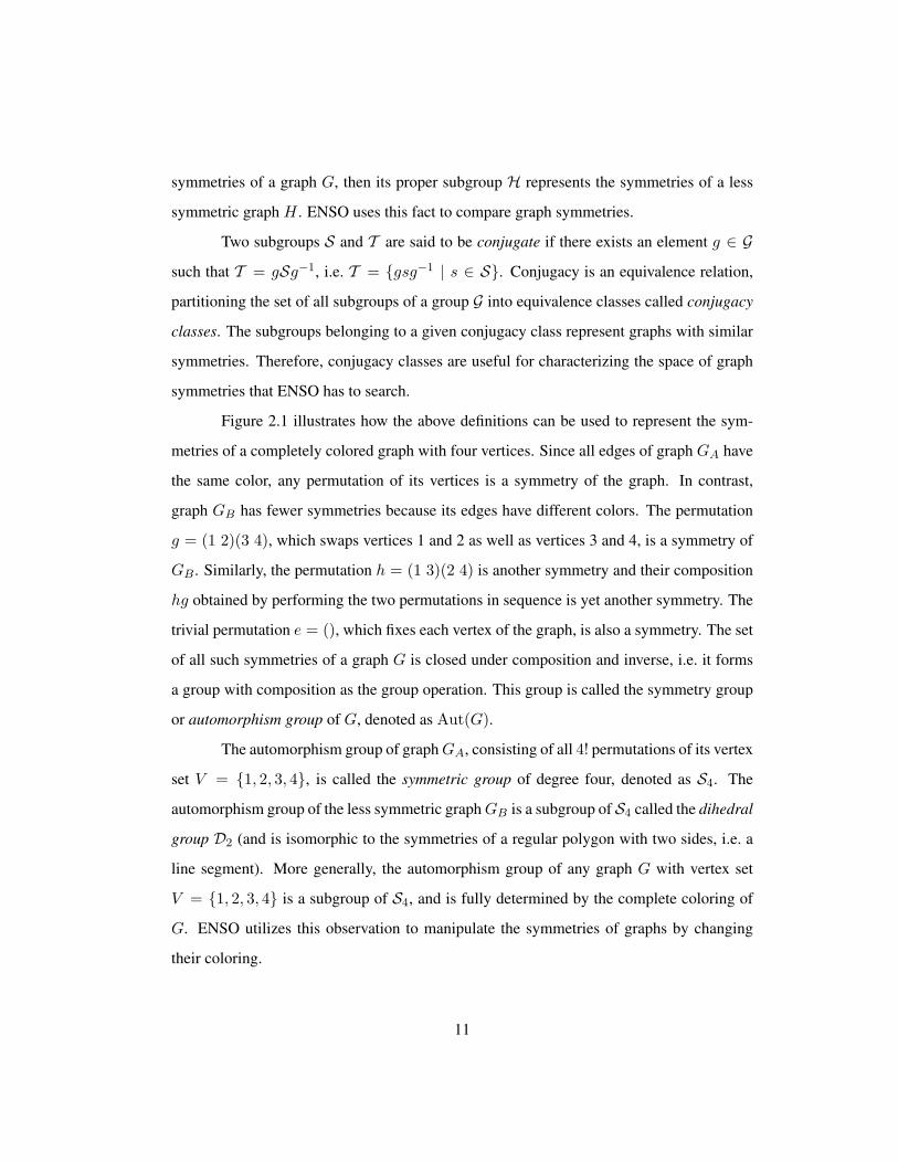
Figure 2.1 illustrates how the above definitions can be used to represent the sym-
metries of a completely colored graph with four vertices. Since all edges of graph GA have
the same color, any permutation of its vertices is a symmetry of the graph. In contrast,
graph GB has fewer symmetries because its edges have different colors. The permutation
g = (1 2)(3 4), which swaps vertices 1 and 2 as well as vertices 3 and 4, is a symmetry of
GB . Similarly, the permutation h = (1 3)(2 4) is another symmetry and their composition
hg obtained by performing the two permutations in sequence is yet another symmetry. The
trivial permutation e = (), which fixes each vertex of the graph, is also a symmetry. The set
of all such symmetries of a graph G is closed under composition and inverse, i.e. it forms
a group with composition as the group operation. This group is called the symmetry group
or automorphism group of G, denoted as Aut(G).
The automorphism group of graphGA, consisting of all 4! permutations of its vertex
set V = {1, 2, 3, 4}, is called the symmetric group of degree four, denoted as S4. The
automorphism group of the less symmetric graphGB is a subgroup of S4 called the dihedral
group D2 (and is isomorphic to the symmetries of a regular polygon with two sides, i.e. a
line segment). More generally, the automorphism group of any graph G with vertex set
V = {1, 2, 3, 4} is a subgroup of S4, and is fully determined by the complete coloring of
G. ENSO utilizes this observation to manipulate the symmetries of graphs by changing
their coloring.
11

GA GB
1 2
3 4
1 2
3 4
Figure 2.1: Representing graph symmetries using groups. Each vertex and edge has a color(indicated by both color and line style) representing a particular combination of parameters. Agraph symmetry is any permutation of vertices under which the edge colors remain the same. Bothgraphs in this figure have vertices of the same color. All edges of graph GA have the same color,while edges of graph GB have different colors. Therefore, any permutation of the vertices of graphGA is a symmetry. In contrast, only the permutations g = (1 2)(3 4) and h = (1 3)(2 4), and theircompositions are symmetries of graph GB . The set of all symmetries of a graph form a group, withcomposition as the group operation. Thus group theory is a natural way to represent symmetries.
Changing the coloring of a graph G such that its new automorphism group is a
subgroup of its original automorphism group is said to break the symmetry ofG. In order to
implement symmetry breaking, ENSO defines a canonical complete coloring of G for any
given automorphism group G using the concept of group action. Formally, the action of G
on the vertex set V is a function G × V → V , denoted (g, v) 7→ g · v for each g ∈ G and
each v ∈ V , which satisfies the following two conditions:
1. e · v = v for every v ∈ V , where e is the identity element of G, and
2. (gh) · v = g · (h · v) for all g, h ∈ G and v ∈ V .
The set of all w ∈ V to which v is mapped by the elements of G is called the orbit of v.
Similarly, the coordinate-wise action of G on V ×V is defined as g ·(v, w) = (g ·v, g ·w) for
any (v, w) ∈ V × V . The orbits in this action are called orbitals, and they form a partition
of V ×V called an orbital partition. Assigning a different color to each part of this partition
produces the desired canonical complete coloring of G.
If a graph G′ is produced by breaking the symmetry of G, then the orbital partition
ρ′ under the action of Aut(G′) is a refinement of the orbital partition ρ under the action of
12

Aut(G), i.e. each part of ρ′ is a subset of a part of ρ. Therefore, the canonical complete
coloring of G′ can be obtained from that of G by assigning new colors to the parts of ρ′
that are a proper subset of a part of ρ and retaining the colors of parts of ρ′ that are also
parts of ρ. ENSO represents this hierarchical relationship between the colors of G and
G′ by organizing the new colors of G′ as the children of colors of G that they replace.
This organization produces a tree of colors when symmetry is broken repeatedly during
evolution.
Breaking symmetry in the above manner induces a partial ordering of the graphs
based on the subgroup relation between their automorphism groups. More precisely, with
subgroup as the partial order relation, the set of all subgroups of a group form a lattice.
Figure 2.2 illustrates this lattice for the subgroups of S4. Nodes of this lattice represent
conjugacy classes of subgroups. A group Gi is placed above another group Gj and con-
nected by a line if and only if Gj is a maximal subgroup of Gi. This lattice contains the
automorphism groups of all completely colored graphs with vertex set V = {1, 2, 3, 4}.
The most symmetric graphs with automorphism group S4 are at the top of the lattice, while
the least symmetric graphs with the trivial automorphism group {e} are at the bottom.
ENSO utilizes this ordering of graphs induced by the subgroup lattice to search the
space of graph symmetries systematically. The above group theory concepts can also be
utilized to explain the symmetries of the two applications considered in this dissertation:
multilegged locomotion and sorting networks. For this purpose, multilegged locomotion is
abstracted as coupled cell systems, as described next.
2.3 Locomotion Controllers
A coupled cell system consists of a set of dynamical systems, called cells, and a specifi-
cation of how the cells are coupled, i.e. how the state of each cell affects the states of the
other cells (Golubitsky and Stewart, 2002). Some or all of the cells and couplings may be
identical, resulting in symmetries that correspond to permutations of the cells under which
13

D43 x
Z43 x D23 x
Z23 x Z26 x
{e}
Z34 x
D2
A4 S34 x
S4
Figure 2.2: Lattice of subgroups of S4. This lattice was computed using the GAP (2007) softwarefor computational group theory and shows the subgroups of the group S4, which is the symmetricgroup of degree four containing all 4! permutations of the set V = {1, 2, 3, 4}. Each node of thelattice represents an equivalence class of conjugate subgroups. There are four types of nodes. Thenode labeled 4×S3 represents the four symmetric groups of degree three obtained by fixing each ofthe four elements of V and permuting only the other three elements. The node labeledA4 representsthe alternating group of degree four, formed by the permutations of V that can be expressed asthe composition of an even number of transpositions. The node labeled Dn represent the dihedralgroups, formed by the permutations of V that are isomorphic to the symmetries of a regular polygonwith n sides. The node labeled Zn represent the cyclic groups, formed by the permutations of Vthat are isomorphic to the group of integers under addition modulo n. The automorphism groupsof all graphs with vertex set V appear in this lattice, inducing a partial order of the correspondinggraphs. Thus, the most symmetric graphs with automorphism group S4 appear at the top and theleast symmetric graphs at the bottom of the lattice, with the trivial automorphism group {e} atthe very bottom. This order makes it possible for ENSO to search the space of graph symmetriessystematically by traversing the lattice from top to bottom.
14

the behavior of the system is invariant. Such symmetric, coupled cell systems can exhibit
synchronous and phase-related periodic patterns in their state. Collins and Stewart (1993)
showed that this patterned behavior can be used to model animal locomotion and to explain
gait symmetries.
Following their method, the modular controllers in this dissertation are also mod-
eled as symmetric coupled cell systems. The patterned oscillatory behavior produced by
these symmetries is independent of the model parameters, i.e. the details of the internal
dynamics of the cells do not matter. Therefore, analyzing the symmetries of a coupled cell
system can give insights into the high-level qualitative behavior of the system.
This analysis is illustrated below for a coupled cell system due to Pinto and Golu-
bitsky (2006). While they used this system to understand biped locomotion, it is adapted in
this review to model quadruped gaits. This system consists of four identical cells, described
by the following system of ordinary differential equations (ODEs):
x1 = F (x1,x2,x3,x4)
x2 = F (x2,x1,x4,x3)
x3 = F (x3,x4,x1,x2)
x4 = F (x4,x3,x2,x1),
(2.1)
where xi ∈ Rk are the k state variables of cell i, and F : (Rk)4 → Rk encapsulates the
internal dynamics of each cell and its coupling with other cells. Thus, this system of ODEs
describes how the state variables of each cell change in time as a function of the cell’s own
state and the state of the other cells.
This system can be represented by the graph in Figure 2.3, which helps visualize
its symmetries. The vertices of the graph represent cells and the edges represent coupling
between the cells. Each edge color represents a different type of coupling, corresponding
to a different argument position in the function F . This graph is the same as the graph
GB of Figure 2.1 in Section 2.2, where its symmetries were analyzed. In particular, its
15

F( , , , )
1 2
3 4
LeftFront
LeftRear
RightRear
RightFront
Figure 2.3: Graph corresponding to the coupled cell system in equation (2.1). The vertices,numbered 1 through 4, represent cells and the edges represent coupling between the cells. Thedifferent edge colors (also indicated with different line styles) represent different couplings, corre-sponding to different argument positions in function F as shown in the legend. This graph helpsvisualize the symmetries of the coupled cell system and shows how the cells may be assigned tocontrol the legs of a quadruped robot to produce different gaits (Figure 1.1). For example, thesesymmetries can constrain cells 1 and 2 to oscillate synchronously with phase opposite to that ofsimilarly synchronous cells 3 and 4, producing the bound gait.
automorphism group is D2, consisting of the symmetric permutations g = (1 2)(3 4),
h = (1 3)(2 4), and their composition hg.
Each symmetry of the graph induces a symmetry of the associated system of ODEs,
i.e. a transformation γ such that γx(t) is a solution whenever x(t) is a solution. For ex-
ample, suppose x(t) is a solution to (2.1). Applying the permutation g to (2.1) produces
an equivalent system of ODEs for which gx(t) is a solution. Thus, the system of ODEs
inherits the symmetry g from the corresponding graph.
In particular, periodic solutions of the system are interesting because they model
gaits. Let x(t) be a T -periodic solution to (2.1) and γ be a symmetry. Then γx(t) is also
a solution. Because solutions to the same initial conditions are unique, if x(t) and γx(t)
are the same trajectory, then their phases must be different, i.e. γx(t) = x(t + θ) where
θ ∈ [0, T ) for all t. Since applying either g twice or h twice to a solution is equivalent to
applying the identity, 2θ ≡ 0 (mod T ) for both symmetries. Therefore, the possible values
of phase shift θ is either 0 or T2 for both symmetries.
Such phase shifts impose constraints on the components of the solution x(t) =
(x1(t),x2(t),x3(t),x4(t)), producing specific patterned behavior for the system. For ex-
16

Pronk Pace Bound Trot
θg 0 T2 0 T
2
θh 0 0 T2
T2
Table 2.1: Gaits corresponding to different combinations of phase shifts θg and θh associatedwith two permutation symmetries g and h of the coupled cell system in Figure 2.3. Thus, thissystem can have solutions modeling a variety of common quadruped gaits.
ample, the bound gait pattern results from the following constraints. The symmetry g is first
applied to x(t) with a phase shift of θg = 0, resulting in the constraints x2(t) = x1(t) and
x4(t) = x3(t). Consequently, the solution has the form x(t) = (x1(t),x1(t),x3(t),x3(t)),
implying that cells 1 and 2 are synchronous and cells 3 and 4 are synchronous, but their syn-
chrony is independent, i.e. it does not yet produce an interesting gait. However, applying
the symmetry h to this solution with a phase shift of θh = T2 results in a further constraint
x3(t) = x1(t+ T2 ). Now, the solution has the form x(t) = (x1(t),x1(t),x1(t+ T
2 ),x1(t+T2 )), implying that cells 1 and 2 are synchronous, while cells 3 and 4 are also synchronous
with the same periodic trajectory as cells 1 and 2, but half-period out of phase. Assigning
these cells to control the legs of a quadruped robot as illustrated in Figure 2.3 produces a
bound gait (Figure 1.1c).
Other common quadruped gaits (such as those depicted in Figure 1.1) can be ob-
tained similarly by selecting different combinations of values for θg and θh as shown in
Table 2.1. Although these gaits are possible solutions of the system, whether any particular
gait can be obtained in an instance of the system depends on the details of the cell dynamics
and the couplings, i.e. on the function F in the ODEs. Chapter 4 shows that this func-
tion F can be designed effectively by utilizing modular neuroevolution, i.e. by representing
each cell as a neural network module and evolving its weights. The resulting controllers
produced all four gaits listed in Table 2.1.
The above theoretical results make the gait-production capabilities of such modular
controller networks easy to understand. Consequently, in contrast to other approaches, these
17

controllers are easy to design and scale well to robots with more legs and more complex
legs (Chapter 4). Moreover, neuroevolution is an effective alternative to designing coupled
cell system ODEs manually such as was done, e.g. by Collins and Stewart (1993),Kimura
et al. (1999), Seo and Slotine (2007), and Righetti and Ijspeert (2008). In Chapter 5, the
ENSO approach extends modular neuroevolution by also evolving the symmetries of the
system. As a result, ENSO can evolve controllers that produce effective gaits even when
such gaits are unknown and manual design of the required symmetries is difficult.
The ENSO approach is useful in problems such as distributed control and multia-
gent systems for which the appropriate symmetries are unknown. In other design problems,
the appropriate symmetry of the solution may be known, and a better approach may be to
construct an optimal solution with that symmetry. The next section discusses an application
for such an approach, i.e. designing minimal-size sorting networks.
2.4 Sorting Networks
A sorting network of n inputs is a fixed sequence of comparison-exchange operations (com-
parators) that sorts all inputs of size n (Knuth, 1998). For example, Figure 2.4 illustrates
a 4-input sorting network. The horizontal lines of the network receive the input values
{x1, x2, x3, x4} at the left. Each vertical line represents a comparison-exchange operation
that takes two values and exchanges them if necessary such that the larger value is on the
lower line. As a result of these comparison-exchanges, the output values appear at the right
side of the network in sorted order: {y1 ≤ y2 ≤ y3 ≤ y4}.
Since the same fixed sequence of comparators in a sorting network can sort any
input, it represents an oblivious or data-independent sorting algorithm, i.e. the sequence
of comparisons does not depend on the input data. Their resulting fixed communication
pattern makes them desirable in parallel implementations of sorting, e.g. on graphics pro-
cessing units (Kipfer et al., 2004). For the same reason, they are also simpler to implement
in hardware and are useful as switching networks in multiprocessor computers (Batcher,
18

Figure 2.4: A 4-input sorting network. The input values {x1, x2, x3, x4} at the left side of thehorizontal lines pass through a sequence of comparison-exchange operations, represented by verticallines connecting pairs of horizontal lines. Each such comparator sorts its two values, resulting inthe horizontal lines contain the sorted output values {y1 ≤ y2 ≤ y3 ≤ y4} at the right. Thosecomparators that are non-overlapping are grouped into parallel steps separated by the vertical dashedlines. This network is minimal in terms of both the number of comparators and parallel steps. Butsuch minimal networks are not known in general for other input sizes and designing them is achallenging optimization problem.
1968). Driven by such applications, sorting networks have been the subject of active re-
search since the 1950’s (Knuth, 1998). Of particular interest are minimal-size networks
that sort utilizing a minimal number of comparators and minimal-delay networks that sort
in minimal number of (parallel) time steps. Designing such networks is a hard combi-
natorial optimization problem, which this dissertation shows how to make more tractable
utilizing their symmetries.
The outputs of any n-input sorting network are invariant to any of the n! permuta-
tions of its inputs because the sorted order at its outputs remains the same. Therefore, it has
symmetry group Sn with respect to permutations of its input variables. Moreover, swapping
the outputs of every comparator in the network to move the larger values to their respective
upper lines creates a dual network producing outputs in reversed sorted order. This duality
can also be expressed formally as symmetries by utilizing the zero-one principle (Knuth,
1998) to represent the network outputs as Boolean functions. According to this principle,
if the network sorts all 2n binary sequences correctly, then it will also sort any arbitrary
19

sequence of n numbers correctly. Therefore, it is possible to represent the network inputs
as Boolean variables and its outputs as Boolean functions of those variables.
The symmetries of the network can then be defined as the symmetries of its set of
output functions. Since the output functions are known, the network symmetries are also
known, making it possible to develop an approach for minimizing the number of compara-
tors in the network by building its symmetries step by step. This approach will be discussed
in Chapter 7.
2.5 Conclusion
Symmetry is ubiquitous in nature and in engineering, imposing constraints on system de-
sign. Nature utilizes these constraints with evolution to search the design space effectively.
A similar approach may be useful with artificial evolution to design complex engineered
systems. This dissertation explores this hypothesis in two domains: (1) designing con-
trollers for multilegged robots, and (2) designing sorting networks with minimal number of
comparators. The next chapter reviews previous research on these topics.
20

Chapter 3
Related Work
Nature utilizes a developmental process to construct organisms from the information en-
coded in their genomes. Constraints for producing regularities and symmetries are en-
coded in the genome as well as in the developmental process itself. Most computational
approaches for evolving symmetry, including ENSO, are based on abstractions of this de-
velopmental paradigm. This chapter begins with a review of these approaches, called indi-
rect encodings. It is followed by a review of previous research on designing controllers for
multilegged robots, a challenging problem that is used in later chapters to evaluate ENSO’s
capabilities to evolve symmetric solutions. The problem of minimizing the size of sorting
networks is also reviewed since it is later used to demonstrate that symmetry constraints
can make combinatorially hard search problems easier to solve.
3.1 Indirect Encodings
Most indirect encodings were developed for evolving artificial neural networks. Kitano
(1990) evolved matrix rewrite rules that produce the adjacency matrix of neural networks
through a series of rewrite steps. His method was based on L-systems, that is, grammatical
string rewrite rules first developed by Lindenmayer (1968) to model the biological growth
21

of plants, yielding complex tree-like structures that resemble fractals. Kitano’s scheme pro-
duced such structures from an initial 2×2 matrix, whose symbols were rewritten iteratively
with other 2× 2 matrices, creating larger and larger matrices. Repeating the symbols in the
matrix creates regularities and symmetries. The rewriting stopped when the current matrix
contained only numerical values, and the result was then interpreted as a neural network’s
adjacency matrix. Kitano evolved such networks to solve encoder/decoder problems. How-
ever, because their size is exponential in the number of rewrite steps, these networks were
typically very large. Evolving detailed connectivity between network units were also diffi-
cult.
Boers and Kuiper (1992) used a different L-system to evolve the topology of mod-
ular neural networks. Their system was based on context-sensitive graph rewriting to de-
scribe neural network topologies. Rule strings were repeated and rules applied recursively
to obtain modular network architectures with symmetries. Boers and Kuiper evolved only
the architecture of the networks in this manner; the connection weights were subsequently
optimized using the backpropagation algorithm (Chauvin and Rumelhart, 1995, Rumelhart
et al., 1986). Using this method, they evolved solutions for problems such as XOR and
shape recognition. Because backpropagation was used for learning the connection weights,
the networks were limited to feed-forward architectures.
Sims (1994a) used another type of generative graph-based encoding to evolve vir-
tual creatures in simulated physical environments. He used directed graphs as genotypes to
encode developmental instructions for constructing the morphology of the creatures. The
nodes of the graph contained information on synthesizing body parts, while its edges spec-
ified the order in which to synthesize them. Multiple edges to the same child node resulted
in reuse of body parts, which is useful for creating multiple instances of limbs and symme-
tries. Recursive edges were also possible, producing repetitive, fractal-like morphologies.
The neural network control circuitry of the creature was embedded in the genotype graph
and evolved along with its morphology. Although the developmental mechanism in this
22

method was elementary, the resulting creatures were significantly regular and often sym-
metry and capable of a variety of interesting locomotive behaviors.
Gruau (1994b), Gruau and Whitley (1993) and Gruau et al. (1996) also used graphs
as genotypes in a method called cellular encoding (CE), which was inspired by the way
biological development occurs through cell division. The genotype encodes a program tree
for constructing a neural network from a single ancestral cell. These program trees were
then evolved using standard techniques for genetic programming (Koza et al., 1996). The
nodes of the tree contained cellular developmental instructions, such as for splitting a cell
into two, deleting a connection between two cells, or changing the weight of a connection.
A full neural network was built by executing these instructions in the sequence specified by
the edges of the program tree. Gruau et al. showed that networks with repeated structures
can be produced by using a recursion instruction that transfers control of development back
to the root of the program tree. He evolved such networks to solve problems with regularity
such as finding the parity and symmetry of a set of binary digits.
Luke and Spector (1996) identified several weaknesses in CE and proposed edge
encoding (EE) as an alternative to address many of those concerns. For example, crossover
in CE can produce drastic changes in the phenotype of an offspring, which may be prob-
lematic for evolution in many domains. Moreover, the networks produced by CE tend to be
highly interconnected because they are grown by splitting cells into two or more intercon-
nected cells. Such networks are a disadvantage in domains where such high connectivity
is not required, requiring the extra weights to be optimized. CE also does not provide a
convenient mechanism to tune connection weights because cells, not connections, are the
target of its development instructions. In contrast, EE grows networks by modifying edges
rather than cells, thereby avoiding these problems of CE and making it more effective in
many domains. However, although both CE and EE are expressive enough to produce all
possible graphs, it is not clear how their particular biases affect their performance on any
given problem.
23

In a domain similar to Sims’ simulated 3D virtual creatures, Hornby and Pollack
(2002) combined ideas of CE and EE with L-systems to evolve the body and brain of such
creatures simultaneously. They used strings of build commands to construct the neural
network brains instead of the trees as in CE. These build commands operate on connec-
tions in the network as in EE. They defined a different set of commands for building body
parts of the creatures. The separate command languages for building the body and brain
were then combined using an L-system, and evolved. The resulting creatures were more
complex, having more parts and regularity, and they were able to walk faster than similar
creatures evolved using a non-developmental encoding. They were also more complex than
the creatures produced by Sims.
Bongard and Pfeifer (2001) also evolved similar virtual creatures, but by using an
abstraction of genetic regulatory networks (GRNs) for encoding bodies and neural net-
works. GRNs model gene expression inside biological cells, i.e. the interactions between
genes as they regulate each other during the production of proteins (Kauffman, 1993). In
Bongard and Pfeifer’s work, the creature begins development as a single spherical unit.
Depending on the concentrations of gene products inside this unit, it grows in size and
eventually divides into two child units. These units are attached to each other by a joint.
Each unit contains a small neural network, which develops according to a variant of the CE
method. In this variant, different gene products trigger different operations that modify the
local network. The development continues until a fixed number of time steps is reached.
Using this method, the authors produced creatures with hierarchical repeated structures in
the task of pushing a block.
Dellaert and Beer (1996) had previously used an abstraction of GRNs called random
Boolean networks (RBNs) to evolve simulated agents capable of following curved lines. In
their method, cells representing the body of the agent developed first. A neural network de-
veloped on top of the arrangement of these cells when specialized cells sent out axons, mak-
ing connections with other cells within its range. A similar neural network developmental
24

model was used by Cangelosi et al. (1994) to create organisms that seek out food and water.
Their networks grew in a two-dimensional space using processes such as cell division and
axon growth. Kodjabachian and Meyer (1998) also used connection growth mechanisms in
their geometry-oriented version of CE called SGOCE. Utilizing similar ideas of develop-
ment, Miller (2004) evolved developmental programs that could construct the French flag
(i.e. adjoining rectangular regions of blue, white, and red colors) and repair damages in it.
In the above methods, small changes in the genotype often produce unpredictable
changes in the phenotypes. Steiner et al. (2009) proposed to reduce this effect by ma-
nipulating the phase space of the dynamic system of the GRN directly. Moreover, GRN-
based approaches abstract biological development at levels lower than those of graph-based
methods by modeling biological growth processes in varying detail. However, detailed sim-
ulation of biological processes are computationally expensive, and may be unnecessary or
even counterproductive (Dellaert and Beer, 1996). Therefore, determining the right level of
developmental abstraction for indirect encodings is an important research topic.
Addressing this issue of abstraction, Stanley (2007) proposed an indirect encoding
called Compositional Pattern Producing Networks (CPPNs) that eliminates the traditional
local interaction and temporal unfolding mechanisms of developmental systems. Instead, he
argued that the effects of such mechanisms can be obtained by composing specific functions
in the appropriate order, i.e. by constructing a CPPN. The patterns produced by a CPPN are
interpreted as the spatial connectivity patterns of a neural network using a method called
HyperNEAT. Stanley et al. (2009) applied this method to tasks having a large number of
inputs and regularities, such as robot food gathering and visual object discrimination.
All the above methods provide mechanisms for reuse of genes and repetition of
phenotypic substructures, thus encouraging modularity. The developmental process also
sometimes produces symmetries in the modular phenotypes, especially if symmetric and
periodic functions are used in the encoding. In contrast, the ENSO approach presented in
this dissertation utilizes symmetry as an organizing principle to constrain other character-
25

istics of development such as reuse and modularity automatically (Chapter 5). As a result,
it can search the space of symmetric solutions effectively by breaking symmetry system-
atically. This claim is evaluated in the task of evolving robust locomotion controllers for
multilegged robots. Previous research on this task is reviewed next.
3.2 Multilegged Locomotion
Efforts to build legged machines began more than a century ago. Early designs required hu-
mans to control the machines, but in the 1970s computer control became a viable alternative
to human control. In the 1980s, Raibert and his coworkers built legged hopping and running
machines (Raibert, 1986, Raibert et al., 1986). They started with a single-legged algorithm
that alternates between a support phase and a flight phase. This algorithm was generalized
to control biped running by alternating support and flight between the two legs. The same
approach was then extended to quadruped gaits in which pairs of legs move in unison (in
pace, bound and trot), by applying the biped algorithm to the paired legs. Thus these early
hand-designed controllers also had symmetric designs with algorithmic modules.
Brooks (1989), another pioneer in robotics, constructed controllers for a six-legged
robot named Genghis incrementally. These controllers were completely decentralized net-
works of augmented finite state machines (AFSMs), some of which were repeated in the
network to replicate the functionality for each leg. Each step of the incremental construction
produced viable controllers for increasingly complex behaviors such as standing up, walk-
ing, and following moving objects. His work also showed that robust walking behaviors
can be produced by distributed sensorimotor control units with limited central coordina-
tion. The controllers that ENSO evolves implement the same idea: Each module produces
control signals for a leg through proprioceptive sensing of joint angles without central co-
ordination.
The distributed nature of legged locomotion has also been observed in insects. Such
observations inspired the distributed neural network hexapod controller hand-designed by
26

Beer et al. (1989). The network uses leaky integrator neurons, each with a different func-
tionality such as sensing and producing rhythmic signals. The controllers produced stable
gaits that are resistant to damage, such as the loss of a sensor or some connections in the
neural network. In another approach, they used a genetic algorithm to find parameter values
for the controller network (Beer and Gallagher, 1992). As in the ENSO approach, the evo-
lutionary search space was shrunk by organizing the controller into subnetworks, producing
a reduced set of parameters for evolution to optimize.
Other approaches to controller design for legged robots typically have a similar fla-
vor, i.e. implementing controllers as continuous-time recurrent neural networks (CTRNNs)
organized into distributed modules. For example, Billard and Ijspeert (2000) hand-designed
CTRNN networks for controlling Aibo robot dogs. Their networks, consisting of oscilla-
tor modules for each joint, were able to walk, trot and gallop. More recently, Tellez et al.
(2006) evolved CTRNNs in the same task. Because of the difficulty of evolving walking
behaviors, network modules were evolved in stages, using more complex fitness evaluations
in each successive stage. Each stage represented a different abstraction of the task, resulting
in a distributed and hierarchical architecture for the controller.
Bull et al. (1995) evolved gaits for their wall-climbing quadruped robot using an
extreme version of distributed control, in which controllers for each leg were modeled as
communicating agents in a multiagent system. They found that such controllers performed
better than a single-agent controller that was responsible for moving all four legs of the
robot. Thus their experiments showed that modular, distributed control (similar to the con-
trollers that ENSO evolves) can be more effective than monolithic control in some domains.
Another approach to evolving modular controllers is based on utilizing the modu-
larity and symmetry produced by indirect encodings. During development of the controller,
the same parts of the program may be read multiple times, once for each module instantia-
tion. When modules are represented intrinsically in the genotype in this manner, evolution
can discover them automatically. Gruau (1994a,b) demonstrated this capability by evolving
27

CTRNN controllers for hexapod locomotion using his cellular encoding (CE) method. Sub-
sequently, Filliat et al. (1999) used SGOCE, the geometry-oriented version of CE, to evolve
CTRNN controllers incrementally for a hexapod, although their scheme required that the
precursor cells for module subnetworks be specified explicitly.
In the above evolutionary methods, fitness of controllers was evaluated by simulat-
ing the physical behavior of robots and their environments. Such experiments are useful
because they allow testing a range of conditions effectively. However, simulation may not
always produce accurate enough results when the evolved controller needs to be transferred
to a physical robot (Jakobi, 1998). In such cases, fitness evaluation must be done using
real robot hardware. Hornby et al. (1999, 2000) for instance did so for the quadruped robot
Aibo. They evolved locomotion parameters for different Aibo gaits by measuring how fast
the robot walked inside a pen. Similarly, Kohl and Stone (2004a,b) obtained faster gaits
for the Aibo by also performing evaluations on physical robots to optimize walk parame-
ters, and Zykov et al. (2004) used hardware evaluations to evolve controller parameters for
a nine-legged robot equipped with pneumatic actuators. In contrast, Miglino et al. (1995)
showed that controllers evaluated using a realistic simulation of the Khepera robot trans-
ferred well to the actual physical Khepera.
The conclusion is that evolution using simulated fitness evaluations can be highly
productive if the simulation is realistic enough and the evolved controllers are robust enough.
Therefore, ENSO evolves robust controllers based on physically realistic simulations. This
approach makes it possible to test a wide range of designs in a wide range of conditions, and
thereby can potentially come up with creative solutions. Moreover, the evolved controllers
produced the same gaits and performed well when they were transferred to a physical robot.
Recent progress in building sophisticated physical robots was summarized by Holmes
et al. (2006). They also discussed the role of mathematical models of body-limb and envi-
ronment dynamics, central pattern generators, and proprioceptive and environmental sens-
ing in the design of a very agile six-legged robot called RHex. The sprawled posture and
28

compliant legs of RHex, inspired by characteristics found in insects, allows the robot to
be stable and operate dynamically even on rocky and uneven terrain (Koditschek et al.,
2004). The stability is achieved through open-loop control utilizing only proprioceptive
feedback. Similarly, the Sprawl hexapedal robot uses open-loop control for stable running
(Clark, 2004). Along the same lines, the modular controllers that ENSO evolves perform
well utilizing only proprioceptive sensing of joint angles.
In nature, the control systems of animals evolved together with their body morphol-
ogy, resulting in tightly integrated, efficient agents. Inspired by this observation, several
researchers have evolved both the controller and the robot morphology concurrently. Ex-
amples of such body-brain evolution include the virtual block creatures of Sims (1994b),
the generative representations used by Hornby and Pollack (2002), and the genetic regula-
tory networks developed by Bongard and Pfeifer (2003). Although not necessarily legged
creatures, the agents produced by such methods may also have modular controllers, and
may be able to walk in a synchronized manner.
Most of the above approaches are motivated by the biological central pattern genera-
tors (CPGs), i.e. groups of neurons that produce oscillatory signals for locomotion (Ijspeert,
2008, Shastri, 1997). They typically implement CPGs as CTRNNs, using leaky integrator
neurons. The modular controller networks that ENSO evolves also function as CPGs, but
they are based on simpler, sigmoidal neurons. Patterned oscillations are still possible in
these networks because they are in essence symmetric, coupled cell systems (Section 2.3).
Theoretically, such systems are CPGs, and in practice, they generate various gaits for legged
robots (Collins and Stewart, 1993). Many researchers have previously hand-designed such
systems using group-theoretic and dynamical systems analysis (Collins and Stewart, 1993,
Kimura et al., 1999, Righetti and Ijspeert, 2008, Seo and Slotine, 2007). In contrast, ENSO
utilizes evolution to design coupled cell systems for multilegged robots automatically.
As discussed in Section 2.3, the symmetries of the coupled cell system determine
the gaits it can produce, making it is necessary to evolve the symmetry together with the
29

n 1 2 3 4 5 6 7 8 9 10 11 12 13 14 15 16m 0 1 3 5 9 12 16 19 25 29 35 39 45 51 56 60
Table 3.1: The least number of comparators m known to date for sorting networks of inputsizes n ≤ 16. Such networks have been studied extensively, but these values of m have been provento be minimal only for n ≤ 8 (shown in bold; Knuth, 1998). Such small networks are interestingbecause they optimize hardware resources in implementations such as multiprocessor switchingnetworks.
weights of the neural network that implements it. In order to search this combined space of
symmetries and network weights effectively, ENSO utilizes symmetry breaking to focus the
search on promising symmetries. While this approach to constraining the search space may
also work in other similar domains, such as distributed controllers and multiagent systems,
another approach may be more appropriate in other domains. For example, the opposite
concept of symmetry building is useful in the challenging problem of finding minimal-size
sorting networks as demonstrated in Chapter 7. Previous research on such networks is
discussed next.
3.3 Sorting Networks
Sorting networks with n ≤ 16 have been studied extensively with the goal of minimizing
their sizes. The smallest sizes of such networks known to date are listed in Table 3.1 (Knuth,
1998). The number of comparators has been proven to be minimal only for n ≤ 8 (Knuth,
1998). These networks can be constructed using Batcher’s algorithm for odd-even merging
networks (Batcher, 1968). The odd-even merge iteratively builds larger networks from
smaller networks by merging two sorted lists. The odd and even indexed values of these
two lists are first merged separately using small merging networks. Comparison-exchange
operations are then applied to the corresponding values of the resulting small sorted lists to
obtain the full sorted list.
Finding the minimum number of comparators required for n > 8 remains an open
problem. The results in Table 3.1, for these values of n, improve on the number of com-
30

Figure 3.1: The 16-input sorting network found by Green. This network has 60 comparators,which is the fewest known for 16 inputs (Knuth, 1998). The network sorts the inputs in 10 parallelsteps, which are separated by dashed vertical lines. The comparators in such hand-designed net-works are often symmetrically arranged about a horizontal axis through the middle of the network.This observation has been used by some researchers to bias evolutionary search on this problem(Graham and Oppacher, 2006) and is also used as a heuristic to augment the symmetry-buildingapproach described in Chapter 7.
parators used by Batcher’s method, and were discovered separately using specialized tech-
niques. For example, the 16-input case, for which Batcher’s method requires 63 compara-
tors, was improved by Shapiro who found a 62-comparator network in 1969. Soon after-
wards, Green found a network with 60 comparators (Figure 3.1), which still remains the
best in terms of the number of comparators.
In Green’s construction, comparisons made after the first four levels (i.e. the first
32 comparators) are difficult to understand, making his method hard to generalize to larger
values of n. For such values, the savings in the number of comparators relative to Batcher’s
method is potentially large. For example, the best known 256-input sorting network due to
Van Voorhis requires only 3651 comparators, compared to 3839 comparators required by
Batcher’s method (Knuth, 1998). Asymptotically, Batcher’s method requires O(n log2 n)
comparators and O(log2 n) parallel steps. In comparison, the AKS network by Ajtai et al.
(1983) produces better upper bounds, requiring only O(n log n) comparators and O(log n)
parallel steps. However, the constants hidden in its asymptotic notation are so large that
31

n 17 18 19 20 21 22 23 24 25 26 27 28 29 30 31 32m 73 80 88 93 103 110 118 123 133 140 150 157 166 172 180 185
Table 3.2: The least number of comparators m known to date for sorting networks of inputsizes 17 ≤ n ≤ 32. Networks for these values of n were obtained by merging the outputs oftwo smaller networks from Table 3.1 using Batcher’s odd-even merging network (Baddar, 2009).Methods used to optimize networks for n ≤ 16 are intractable for these values of n because of theexplosive growth in the size of the search space. As a solution, the symmetry-building approachdescribed in Chapter 7 mitigates this problem by constraining search to promising solutions andimproves these results for input sizes 17, 18, 19, 20, and 22.
these networks are impractical. In contrast, Leighton and Plaxton (1990) have shown that
small constants are actually possible in networks that sort all but a superpolynomially small
fraction of the n! input permutations.
Therefore, in order to create networks that sort all n! input permutations for large
values of n, Batcher’s odd-even merging algorithm is often used in practice, despite its non-
optimality. For example, such networks for 17 ≤ n ≤ 32 listed in Table 3.2 were obtained
by merging the outputs of two smaller networks from Table 3.1 using an odd-even merging
network (Baddar, 2009).
The difficulty of finding such minimal sorting networks prompted researchers to
attack the problem using evolutionary techniques. In one such study by Hillis (1991), a
16-input network having 61 comparators and 11 parallel steps was evolved. He facilitated
the evolutionary search by initializing the population with the first four levels of Green’s
network, so that evolution would need to discover only the remaining comparators. This
(host) population of sorting networks was co-evolved with a (parasite) population of test
cases that were scored based on how well they made the sorting networks fail. The purpose
of the parasitic test cases is to nudge the solutions away from getting stuck on local optima.
Juille (1995) improved on Hillis’ results by evolving 16-input networks that are as
good as Green’s network (60 comparators in 10 levels), from scratch without specifying
the first 32 comparators. Moreover, Juille’s method discovered 45-comparator networks for
the 13-input problem, which was an improvement of one comparator over the previously
32

known best result. His method, based on the Evolving Non-Determinism (END) model,
constructs solutions incrementally as paths in a search tree whose leaves represent valid
sorting networks. The individuals in the evolving population are internal nodes of this
search tree. The search proceeds in a way similar to beam search by assigning a fitness
score to internal nodes and selecting nodes that are the most promising. The fitness of an
internal node is estimated by constructing a path incrementally and randomly to a leaf node.
This method found good networks with the same number of comparators as in Table 3.1 for
all 9 ≤ n ≤ 16.
Motivated by observations of symmetric arrangement of comparators in many sort-
ing networks (Figure 3.1), Graham and Oppacher (2006) used symmetry explicitly to bias
evolutionary search. They compared evolutionary runs on populations initialized randomly
with either symmetric or asymmetric networks for the 10-input sorting problem. The sym-
metric networks were produced using symmetric comparator pairs, i.e. pairs of comparators
that are vertical mirror images of each other. Although evolution was allowed to disrupt the
initial symmetry through variation operators, symmetric initialization resulted in higher
success rates compared to asymmetric initialization. A similar heuristic is also utilized to
augment the symmetry-building approach in Chapter 7.
Evolutionary approaches must verify that the solution network sorts all possible in-
puts correctly. A naive approach is to test the network on all n! permutations of n distinct
numbers. A better approach requiring far fewer tests utilizes the zero-one principle (Sec-
tion 2.4) to reduce the number of test cases to 2n binary sequences. However, the increase
in the number of test cases remains exponential and is a bottleneck in fitness evaluations.
Therefore, some researchers have used FPGAs to mitigate this problem by performing the
fitness evaluations on a massively parallel scale (Korenek and Sekanina, 2005, Koza et al.,
1998). In contrast, the symmetry-building approach in this dissertation utilizes Boolean
lattices to evaluate fitness efficiently.
33

3.4 Conclusion
Previous research on utilizing symmetry in evolutionary search have focused on indirect en-
codings, which are abstractions of development in nature. However, searching large design
spaces efficiently by utilizing symmetry to constrain search has been difficult because sym-
metries are difficult to specify formally in such systems. The ENSO approach will addresses
this issue by utilizing group theory to represent symmetry mathematically. This capability
will then be utilized to evolve robust controllers for multilegged robots, a hard engineering
problem that has been investigated since the 1970s. Moreover, the general principle of uti-
lizing symmetries to constrain search will be demonstrated on another challenging problem
that has received considerable attention in the literature, i.e. designing minimal-size sorting
networks.
34

Chapter 4
Evolving Modular Controllers
It is sometimes possible to constrain large search spaces by hand-designing symmetries.
For example, the symmetries of modular neural network controllers for multilegged loco-
motion on flat ground can be designed in this way (Sections 2.3 and 3.2). This chapter
evaluates how effective the resulting search is by evolving walking behaviors for a simu-
lated quadruped robot. Three types of controllers were tested: (1) hand-designed controllers
that serve as a baseline for performance comparisons, (2) non-modular controllers uncon-
strained by symmetry (i.e. the parameters of the entire neural network are evolved at once),
and (3) modular controllers constrained by symmetry (i.e. only one module is evolved and
duplicated four times to produce the complex neural network controller).
4.1 Quadruped Robot Model
The robot model resembles a table with a rectangular body supported by legs at the four
corners (Figure 4.1). The legs are cylindrical with capped ends, and attached to the body
by a hinge joint that has a full 360° freedom of rotation. The axis of rotation of the joint is
tilted to the side, causing the rotating leg to trace a cone. The leg makes contact with the
ground when it is at one edge of the cone. Forward or backward locomotion is achieved
35

Figure 4.1: The quadruped robot model. The legs are attached to the body by hinge joints withaxes of rotation tilted sideways, allowing the legs to make full circular rotation. Locomotion isachieved by coordinating the circular movements of the legs. This model is a simple but physicallyrealistic platform that also allows scaling up to more complex robots by adding more legs or byincreasing the legs’ degrees of freedom.
by coordinating the circular movements of the leg. The controller activates the simulated
servo motor attached to each joint by specifying either the desired joint angle or the angular
velocity (in different experiments).
This model can be generalized and made more complex by adding more legs to
the table or by using joints that have more degrees of freedom, such as a universal joint.
Such more complex robots will be used to test the scale-up properties of the approach in
Sections 4.8 and 4.9.
4.2 Hand-Designed Controller
The hand-designed controller specifies the desired angular positions of the legs as functions
of time, coordinated so as to obtain a trot gait (Figure 1.1d). Plotted over time, the leg
angles for the quadruped robot model produce sawtooth waveforms that all have the same
period (Figure 4.2). The waveforms of the diagonal leg pairs are synchronous, and a half-
36

-240
-180
-120
-60
0
60
120
180
240
0 2 4 6 8 10
Leg
Join
t Ang
le (d
eg)
Time (s)
LF and RR RF and LR
Figure 4.2: Leg angles specified by the hand-designed controller. Plotted over time, these legangles produce sawtooth waveforms, i.e. the legs rotate with constant angular velocity. The diagonalpairs of legs move in unison, but each pair moves a half-period out of phase with the other pair,producing a trot gait.
period out of phase with the other pair. This gait is an effective base gait that occurs often
in nature, and the evolved gaits can be compared with it.
4.3 Non-modular Controller
Figure 4.3a illustrates the non-modular neural network controller for the quadruped robot.
Although a variety of architectures are possible, this simple two-layer architecture was
chosen to make a fair comparison to the symmetric modular controller. The inputs are the
angular positions of the leg joints, and the outputs are the desired angular velocities of the
legs. Each input unit is connected to all hidden units, but each output unit is connected
only to two hidden units, which in turn send their activation exclusively to that output unit.
The hidden and output units have sigmoidal activation functions with a bias and slope as
parameters; the input units do not perform any computation. Since the genotype of the non-
modular controller represents the entire network, all parameters of the network will have to
be optimized through evolution.
37

(a) Non-modular controller network
(b) First module of the modular controller network
Figure 4.3: Genotypes of the non-modular and modular controller networks for thequadruped robot model. Inputs are the leg angles and outputs are the desired angular velocities.Both the non-modular and modular networks have the same architecture. However, the genotypeof the non-modular network contains the entire network while that of the modular network containsonly the first module. The full modular network is constructed by replicating the first module withdifferent permutations of the inputs.
38

A more general robot model having additional joint angles requires a network with
additional inputs and outputs to represent those angles. The number of hidden nodes will
also need to be increased to achieve better performance on more complex robots, thus in-
creasing the search space and making the controller more difficult to optimize.
4.4 Modular Controller
The non-modular network can be decomposed structurally into four subnetworks (mod-
ules), each containing one of the output units, the two hidden units from which the out-
put unit receives activation, and all the input units. Constraining these subnetworks to be
identical with the same interconnection pattern as in Figure 2.3 results in a modular neu-
ral network with the same symmetries. Only the first subnetwork is used as the genotype
(Figure 4.3b), making the evolutionary search space one-fourth of that for non-modular
evolution. The full modular network is obtained by instantiating the other subnetworks
with copies of the first subnetwork and with appropriate permutations of the inputs. As a
result, the output unit of each subnetwork computes the time derivative of the joint angle it
controls as a function of all the joint angles.
Such a construction allows the modular network to be modeled as a coupled cell
system. The modules correspond to cells, and the input connections of modules correspond
to couplings. Since the modules are identical, the cells are also identical. The permutations
of module inputs determine how cells are coupled to each other. These permutations are
chosen such that the system of ODEs corresponding to the resulting coupled cell system
has the same form as equation (2.1). In this formalism, xi represents the joint angles for leg
i, and F represents the functional equivalent of each neural-network module.
Analysis of the symmetries of equation 2.1 and its corresponding graph (Figure 2.3)
in Section 2.3 showed that this coupled cell system can have periodic solutions that corre-
spond to synchronous and phase-related oscillatory behavior of the cells. When these cells
(i.e. module outputs) are assigned to control robot legs, symmetric and regular gaits are
39

obtained. With such a setup, neuroevolution can exploit the symmetries and discover an
appropriate F that produces effective gaits.
This coupled cell system models the behavior of the controller only; it does not
take into account the dynamical effects of the robot and the environment in which the robot
operates. Such effects may be thought of as perturbations to the state variables of the sys-
tem, and the evolved controllers must be robust against them. Evolution can also discover
a controller that utilizes such perturbations as feedback for switching to more suitable gaits
on difficult terrains, as observed in Section 4.7.
Experiments comparing the controllers produced by the above three methods were
run on flat ground and on terrain with obstacles, and on robots with different number of
legs and different number of joint degrees of freedom. Visualization videos of the walking
behaviors produced in these experiments can be seen at the website http://nn.cs.
utexas.edu/?modularne.
4.5 Experimental Setup
The experiments were implemented utilizing a number of open source tools. The neu-
roevolution code was implemented as a library layer on top of the Open BEAGLE (2007)
evolutionary computing framework, taking advantage of its generic programming interface.
The physics simulation was programmed using OPAL (2007), an abstraction library on top
of the Open Dynamics Engine (ODE, 2007). The Object-Oriented Graphics Rendering
Engine (OGRE, 2007) library was used for 3D visualization of the simulation.
The initial population of networks was created with connection weights chosen ran-
domly from the range [−2, 2), neuron biases set to 0, and neuron sigmoid slopes set to 1.
Three types of mutations were used, one for each of the above parameter types: (1) weight
mutations, (2) bias mutations, and (3) slope mutations. All three types were implemented
as Gaussian perturbations (with σ = 0.2), acting with a specified probability (0.5) on each
of the parameters belonging to that type. In each generation, an offspring was created by
40

first selecting a parent in a two-way tournament and then applying exactly one of the three
mutation types, chosen with equal probability. In addition, the network with the best fitness
was copied without change to the next generation. A population size of 200 was used in all
experiments.
Each network was evaluated in a physically realistic simulation in which the net-
work controlled the locomotion of a robot. When the robot was initially placed in the
simulation environment, its longitudinal and lateral axes were aligned with the coordinate
directions of the ground plane. The simulation was then carried out for one minute of
simulated time with step size 0.01s, after which the fitness of the controller network was
calculated as the maximum distance traveled by the robot along either of the two coordinate
dimensions (i.e. the Chebyshev distance; Murtagh, 2002). This fitness measure ensured that
the evaluation of controller networks was fair even on the terrain with bumps arranged in
concentric squares (Section 4.7). Although appropriate as a quantitative measure of perfor-
mance, this measure does not capture how good the controllers are qualitatively. Therefore,
the resulting gaits were also visualized and evaluated manually at the end of evolution to
confirm that the champion controller networks had good locomotive properties.
For all experiments, evolution was run for 500 generations and repeated 10 times,
each time with a different random number seed. The average and standard deviation of
champion network fitness over all experiments are plotted in Figure 4.4. The fitness of the
hand-designed controller is also plotted for comparison. This controller was obtained by
manually implementing domain knowledge as well as by experimenting with gait periods
similar to those produced by the modular controllers. The following sections discuss the
results of each experiment in detail.
4.6 Walking on Flat Ground
In the first experiment, networks were evolved to control the simulated quadruped robot
on flat terrain. The modular networks performed significantly better than the non-modular
41

0
20
40
60
80
100
120
140
0 100 200 300 400 500
Fitn
ess
Generations
modularnon-modular
hand-designed
(a) Quadruped robot with hinge joints on flat terrain.
0
10
20
30
40
50
60
70
0 100 200 300 400 500
Fitn
ess
Generations
modularnon-modular
hand-designed
(b) Quadruped robot with hinge joints on obstacle terrain.
Figure 4.4: Performance of hand-designed, modular, and non-modular neuroevolution con-trollers on different terrains and robot models. Bold lines are averages and the shaded regionson either side are standard deviations obtained over 10 trials of evolution. The fitness of the hand-designed controller is also shown for reference. (a) Modular controllers perform significantly betterthan both non-modular and hand-designed controllers in the baseline experiment. (b) Performancegap between modular controllers and hand-designed controllers increases significantly when obsta-cles are added to the environment.
42

0
20
40
60
80
100
120
0 100 200 300 400 500
Fitn
ess
Generations
modularnon-modular
hand-designed
(c) Hexapod robot with hinge joints on flat terrain.
0
50
100
150
200
250
0 100 200 300 400 500
Fitn
ess
Generations
modularnon-modular
hand-designed
(d) Quadruped robot with universal joints on flat terrain.
Figure 4.4: (cont.) (c) Similarly, the performance gap increases significantly when number of legsis increased to six. (d) Likewise, performance gap increases significantly when an angular degree offreedom is added to each leg joint. These results demonstrate the advantage of modular evolution,i.e. search constrained by symmetries, over non-modular evolution and hand-design in discoveringcontrollers for multilegged robots.
43

networks through all generations, as illustrated in Figure 4.4a. This result implies that
the robots with modular controllers are able to travel farther than those with non-modular
controllers. Figure 4.4a also shows that the modular controllers have higher fitness than
the hand-designed controller. This result means that through evolution it was possible to
discover more efficient or better tuned gaits than could be designed by hand.
When the locomotion of champion networks were visualized, another important
benefit of modular evolution was revealed. The modular controllers produce regular gaits,
such as pronk, pace, bound and trot, similar to those found in animals. Its hand-designed
symmetries constrain the search space, making it easy to evolve such gaits (Section 2.3).
In contrast, the non-modular networks typically produce asymmetric gaits in which one or
two legs have limited mobility, resembling the gaits of crippled animals.
These results establish a baseline for comparisons involving more difficult terrain
and more complex robots, as described next.
4.7 Negotiating Obstacles
In the next experiment, obstacles in the form of bumps (or walls, or fences) were placed on
the ground at regular intervals to make the task of the controller more difficult (Figure 4.5).
Five bumps were used in each coordinate direction, together forming concentric squares
aligned with the coordinate directions of the ground plane. The first bump was at 10 units
from the center, and the remaining bumps were at every 5 units outward. The robot was
initially placed at the center. Note that although moving in a skewed direction can cover
more distance without encountering the bumps, it does not increase the Chebyshev distance
measure that is used as fitness.
As in the experiment on flat terrain, the modular controllers have a clear advantage
over non-modular and hand-designed controllers because of their symmetry (Figure 4.4b).
The hand-designed controller has a particularly hard time: It is unable to get past the first
or second bump, depending on how the legs initially hit the bumps. This result further
44

Figure 4.5: Robot negotiating a terrain with obstacles. The obstacles consist of five equallyspaced bumps forming concentric squares around the robot. Moving on this terrain by stepping overthe bumps is a difficult task: The symmetries of the modular controller make it possible to performthis task effectively, whereas the non-modular and hand-designed controllers struggle. Visualizationvideos of such behaviors can be seen at http://nn.cs.utexas.edu/?modularne.
demonstrates how evolution can discover more effective behavior than can be achieved
through hand design.
The bumps perturb the dynamics of the modular controller more than the flat ground
does. As a result, evolution often discovers controllers that utilize these perturbations to
transition to a more favorable gait for stepping over the bumps. An example of this phe-
nomenon is shown in Figure 4.6, where the robot changes from bound to trot when it hits the
first bump, allowing it to get over it more easily. Such behaviors can potentially be general-
ized to arbitrary environments by evolving modular controllers with additional sensors, e.g.
for obstacles, that can signal the need for gait transitions more reliably than perturbations
of controller dynamics. In contrast, non-modular evolution fails to evolve gait transitions
most likely because it does not have any symmetry constraints.
45

-240
-180
-120
-60
0
60
120
180
240
7 8 9 10 11 12 13 14 15
Leg
Join
t Ang
le (d
eg)
Time (s)
LF RF LR RR
Figure 4.6: Gait changes produced by an evolved modular controller on a terrain with ob-stacles. As in Figure 4.2, the plot shows angular positions of the four legs of the robot over time.Initially, the front pair of legs (LF and RF) move out of phase from the rear pair (LR and RR), i.e.the robot has a bound gait (Figure 1.1c). The robot encounters the bumps at about 10 seconds. Asit tries to move forward, its legs hit the bumps repeatedly, perturbing the dynamics of the controller.These perturbations cause the controller to transition to a trot gait in which the diagonal pairs oflegs move out of phase (Figure 1.1d). This change of gait makes it easier for the robot to step overthe bumps. Thus modular neuroevolution can evolve controllers that have the flexibility to negotiatedifficult terrain.
46

Figure 4.7: The hexapod robot model. This model is obtained by extending the quadruped inFigure 4.1 with a third row of legs. It is used to test how well the different methods for designingcontrollers scale-up to robots with more legs.
4.8 Scaling to a Hexapod
Because of the symmetries of the modular controller, only one module needs to be encoded,
receiving input from all legs. Therefore, when more legs are added to the robot model,
only a few more parameters need to be added to the modular genotype. In contrast, the
non-modular genotype needs significantly more parameters because it encodes all modules
separately. Consequently, evolutionary search is likely to be harder for the non-modular
method than for the modular method when the number of legs is increased.
This hypothesis was tested by evolving controllers for a hexapod robot that had
equally spaced rows of legs along its longitudinal axis (Figure 4.7). A hand-designed con-
troller was also built by generalizing the trot gait of the quadruped into a tripod gait, in
which the front and rear legs of one side are in phase with the middle leg of the other
side. The coupled cell system associated with the hexapod modular controller extends the
quadruped system of Figure 2.3, and is obtained by adding a third row of cells and con-
necting them with the other cells using bidirectional links (Figure 4.8). The resulting cell
system has two types of symmetries: (1) swapping of the left and right columns of cells,
and (2) cycling of the rows of cells either up or down.
47

1 2
3 4
LeftFront
LeftMiddle
RightMiddle
RightFront
5 6LeftRear
RightRear
to/from cells 1 and 2
to/from cells 5 and 6
Figure 4.8: Graph of the coupled cell system for the hexapod robot in Figure 4.7. This systemextends the quadruped system of Figure 2.3 by adding a third row of cells and connecting them withthe other cells using bidirectional links. The resulting symmetries make the graph invariant to (1)swapping the left and right columns of cells and (2) cycling the rows of cells up or down. Thesesymmetries constrain the oscillations of the system, making it possible to evolve effective hexapodgaits similar to those in nature.
Fitness of the modular and non-modular controllers in this experiment are plotted in
Figure 4.4c. The modular controllers now outperform the non-modular and hand-designed
controllers with a wider performance gap than in the quadruped case in Figure 4.4a. The
non-modular controllers perform at the same level as the hand-designed controllers, pos-
sibly because they only have to get a few legs moving in a coordinated fashion to make
reasonable progress. On the other hand, the modular controllers produce gaits with sym-
metric leg movements, typically producing a longitudinal wave pattern with same-row legs
in phase or a half-period out of phase, which is much more effective and similar to the hexa-
pod gaits in nature. Thus the symmetry constraints of modular evolution make it possible
to scale up better than non-modular evolution when more legs are added to the robot.
48

4.9 Scaling to Universal Joints
The robot can also be made more complex and more difficult to control by increasing the
number of angles that has to be controlled in each leg. That is, while the legs trace a
cone in the previous robot models, a more challenging model would require controlling
the forward-backward (longitudinal) and sideways (lateral) rotations of the legs separately.
Since the controller inputs are the joint angles, the number of input connection weights
increases correspondingly. This increase is limited to the single genotype module for mod-
ular networks, while it gets multiplied by the number of joints for non-modular networks.
Again, because of the large number of extra parameters that non-modular evolution has to
search, finding a good controller is likely to be harder for non-modular than for modular
evolution.
The final experiment tested this hypothesis by replacing each hinge joint of the
quadruped robot with a universal (hip) joint. This change in the robot model doubles the
number of degrees of freedom of each joint and, consequently, the number of controller
inputs. The forward-backward rotation is limited to 30° in both directions and the sideways
rotation from vertical to 45° outwards. The hand-designed controller is generalized to this
setup by adding signals for the lateral angle of each leg such that it is a quarter-period out
of phase with its longitudinal angle, producing a trot gait.
The above hypothesis is confirmed by Figure 4.4d. The performance gap between
modular and non-modular evolution has widened significantly: Modular evolution now per-
forms nearly four times better than non-modular evolution, and also slightly better than the
hand-designed controller. Visualizing the gaits reveals that non-modular controllers typi-
cally produce gaits resembling severely crippled animals, with nearly all their legs appear-
ing disabled and poorly coordinated. These robots often have sideways moving gaits and
may have certain joint angles locked in a fixed position. The modular controllers, on the
other hand, typically produce regular trot gaits that achieve high fitness.
49

Thus unlike non-modular evolution, modular evolution scales up well when the
robot legs are made more complex. These results demonstrate that utilizing symmetries
to constrain the search space makes it possible to scale up evolutionary search to more
complex robots.
4.10 Conclusion
This chapter showed how the symmetries of modular controllers constrain evolutionary
search, reducing the number of parameters that need to be optimized and thus making it
possible to find effective solutions. These symmetries were hand-designed to make it pos-
sible to evolve common quadruped gaits found in nature such as pronk, pace, bound, and
trot. The modular controllers also evolved the ability to change gaits in response to changes
in the environment and to scale well to more complex robot morphologies. In contrast,
the unconstrained search of non-modular evolution failed to evolve effective controllers.
However, designing symmetries by hand to constrain search in this manner is not always
possible, making it necessary to evolve the symmetries as well, as will be discussed in the
next chapter.
50

Chapter 5
Evolving Controller Symmetries
As the last chapter demonstrated, utilizing symmetries to constrain the search space makes
it possible to evolve effective solutions that are otherwise difficult or impossible to find.
However, it is not always possible to determine the appropriate symmetry analytically. For
example, the hand-designed symmetries utilized in the last chapter are no longer appropriate
when the robot is walking on an incline, because the physics is different. Continuing in the
robot control domain, this chapter extends modular neuroevolution to evolve symmetries
as well. The key insight is to utilize group theory to keep the search space constrained to
promising solutions while making it possible for evolution to explore different symmetries
by breaking symmetry systematically.
5.1 Symmetry-Breaking Approach (ENSO)
This approach, called Evolution of Network Symmetry and mOdularity (ENSO), evolves
both the symmetries and the weights of modular neural networks simultaneously. ENSO
represents the modules and the connections between the modules as vertices and edges of
a completely colored graph (Section 2.2). Since such graphs have an ordering induced by
the subgroup lattice of their automorphism groups, ENSO evolves symmetries by traversing
51

this lattice from top to bottom. As a result, it searches the space of symmetries systemat-
ically from the most symmetric to the least symmetric, breaking symmetry minimally in
each step to constrain search to promising graphs. Moreover, ENSO searches the space
of network weights for each subgroup visited in the lattice. Therefore, evolving the graph
representations of such modular networks consists of two components: (1) evolving the
symmetries of the module interconnection graph and (2) evolving the connection weights
within and between modules. These components are described below.
5.1.1 Symmetry Evolution
In order to evolve a network with n modules, ENSO initializes a population of maximally
symmetric, completely colored graphs with vertex set V = {1, 2, . . . , n}, that is, graphs of
automorphism group Sn. These graphs have only two colors: All vertices are of one color
while all edges are of the other color. Vertices and edges with the same color have the same
set of neural network parameters and are therefore considered identical. Therefore, each
graph in the initial population represents a modular neural network with identical modules
and identical connections between the modules.
ENSO computes the subgroup lattice of Sn and the orbital partitions for each sub-
group in the lattice at the beginning of evolution using the GAP (2007) software. During
evolution, ENSO utilizes this lattice to mutate the coloring of graphs, thus breaking their
symmetry. Each such color mutation creates a new graph coloring from the orbital partition
of a randomly chosen successor in the subgroup lattice; that is, the automorphism group of
the mutated graph is a random maximal subgroup of the automorphism group of the original
graph.
ENSO organizes the colors created by successive color mutations as a tree. Each
tree is a genotype for evolution. The leaf colors of the tree specify the complete coloring of
a graph, which is the phenotype that is constructed from the genotype. Each genotype tree
of the initial population has two leaf nodes, one representing the color of vertices and the
52

other representing the color of edges (Figure 5.1a). These two leaf nodes are the children
of a root node that represents a dummy color.
Thus each node in the genotype tree represents a particular color c. Second, it
represents the set Q of elements of V ×V (i.e. the set of vertices or edges of the phenotype
graph) that have the color c. This representation is a bit string of length n2, where the bit
position (i− 1)n + j is set to 1 if and only if the pair (i, j) is in Q. Third, the node stores
the neural network parameters of these elements, i.e. the biases and connection weights of
the module network (for each vertex) or the connection weights between modules (for each
edge).
The effect of a color mutation on the genotype tree is to partition the set of vertex
and edge elements associated with one or more leaf nodes, creating a new child color for
each part of the partition (Figure 5.1b). As a result, the colors of these elements change
correspondingly in the phenotype graph, i.e. some of the elements that were identical be-
fore the mutation are no longer identical: A new (initially random) set of neural network
parameters is associated with each new color. These color changes break the symmetry of
the phenotype graph, i.e. it loses its color invariance under a subset of permutations that
were its symmetries prior to the mutation.
Since the automorphism group of the mutated graph is a maximal subgroup of the
automorphism group of the original graph, color mutations break symmetry in minimal
increments. As a result, evolution searches the space of symmetries systematically by ex-
ploring more symmetric graphs before less symmetric ones. Creating new colors and pa-
rameters in the genotype tree during this process increases the complexity of the genotype,
that is, evolution searches in a low-dimensional space before it complexifies into a higher
dimensional space. This approach allows evolution to optimize solutions in a small search
space, and elaborate on them by adding more dimensions. Such complexification has been
demonstrated to be useful in other methods for evolving neural networks (Siebel and Som-
mer, 2007, Stanley and Miikkulainen, 2004). Complexification also means that simpler
53

PhenotypeGenotype
V x V:Params:
1111111111111111
p1,...,pk q1...,qm
Nil
Params: Params:
ColorMutation
(a)
(b)
Edges: 0111101111101110Vertices:1000010000100001
V x V:Params:
1111111111111111
p1,...,pk q1...,qm
Nil
Params: Params:Edges: 0111101111101110Vertices:1000010000100001
r1,...,rm s1...,smParams: Params:Edges: 0101101001101010Edges: 0010000110000100
x1 x2 x3 x4
y1
Module 1
Network module
x1 x2 x3 x4
y1
Module 1
1 2
3 4
1 2
3 4
Figure 5.1: Examples of genotype, phenotype, network module, and color mutation. ENSOuses a tree of colors as genotype (left). Each leaf of this tree has a unique color, and representsa set of vertices or edges of the phenotype graph (middle) that have the same parameter values.The vertices and edges of the phenotype graph represent the modules of a neural network and theconnections between them (right). Their parameters (stored in the genotype) consist of node biasesand connection weights for each module network (vertex) and weights for each connection betweenmodules (edge). Each module has a fixed architecture with a layer of hidden nodes fully connectedto its inputs and outputs. A connection from another module (not shown) is implemented by fullyconnecting its input layer to the hidden layer of the target module. (a) At the beginning of evolution,each genotype in the population represents a maximally symmetric phenotype graph with automor-phism group S4. All vertices of this graph have the same color (solid black, represented by the leafon the left) and all its edges have the same color (orange with alternating dots and dashes, repre-sented by the leaf on the right), implying that all modules are identical and all connections betweenthem are also identical. (b) A color mutation breaks the phenotype graph symmetry to D4, whichis a maximal subgroup of S4 (Figure 2.2). As a result, two child nodes are created for the noderepresenting the set of edges, i.e. the set of edges is partitioned into two and each part is coloreddifferently (dotted blue and dashed green). Since each color is associated with a different combina-tion of parameter values, the mutated phenotype graph represents two types of connections betweennetwork modules. Such color mutations constrain symmetry search, and together with parametermutations, make it possible to evolve symmetric modular neural networks efficiently.
54

solutions are preferred over more complex solutions, thus conforming to the principle of
Occam’s razor, which often results in more robust neural networks (Fahlman and Lebiere,
1990, le Cun et al., 1990).
For each phenotype graph that ENSO produces in the above manner, it also evolves
the neural network parameters associated with its colors to optimize the functionality of
the network modules and their interconnections. The structure of these modules and the
evolution of network parameters are described next.
5.1.2 Module Evolution
A fixed architecture is used for the neural network modules, each module consisting of a
layer of hidden nodes that are fully connected to inputs and outputs (Figure 5.1). Evolution
optimizes two kinds of network parameters: (1) the scalar parameters of these modules, i.e.
the connection weights and node biases, which form the vertex parameters of the phenotype
graph, and (2) the weights of connections between modules, which form the edge parame-
ters of the phenotype graph. Module interconnections are implemented by fully connecting
the input layer of one module to the hidden layer of the other module (for instance, in a
legged locomotion controller, such interconnections allow the control module of one leg to
receive the state of another leg as input). If modules are not connected, then the correspond-
ing graph edges are disabled using special binary edge parameters.
The vertex and edge parameters of the phenotype graph are stored in the genotype
leaf nodes. In the initial population, these parameters are initialized with random values in
parameter-specific ranges specified by the experimenter. During evolution, ENSO mutates
each of these parameters probabilistically by perturbing them with Gaussian noise. When a
parameter in a particular genotype node is mutated, it affects all vertices and edges with that
color. Thus, representing identical elements by a single node in the genotype tree allows
evolution to search the parameter space efficiently by making coordinated changes to the
phenotype.
55

Symmetry and modules must be evolved together to find solution networks, making
it necessary to mix parameter and color mutations. However, color mutations produce
severe changes in the phenotype, resulting in sudden changes in fitness that may cause
the phenotype to be removed from the population. It is possible to determine how effective
such structural changes are only after enough parameter mutations have accumulated over
evolutionary time. Therefore, color mutations are given the opportunity to be optimized by
creating population niches, similar in spirit to speciation in the NEAT algorithm (Stanley
and Miikkulainen, 2004) and to the evolution of structure and parameters at different time
scales in the EANT/EANT2 algorithm (Siebel and Sommer, 2007). Individuals occupying
a niche have the same phenotype symmetry and remain in the niche for a certain number
of generations before they compete with the rest of the population. This number is a linear
function of the size of the genotype, allowing individuals with more parameters to stay in
their niches longer. Protecting symmetry mutations using this niching mechanism improves
evolutionary performance significantly.
Evolving the symmetries and parameters of modular neural networks in the above
manner constrains search to explore promising regions of the subgroup lattice and corre-
sponding parameter combinations. As a result, ENSO can find solutions to modular prob-
lems effectively, as demonstrated next.
5.2 Quadruped Controller
ENSO evolved modular controllers for the quadruped robot model described in Section 4.1.
Although robots with more legs and complex legs can be used, this chapter focuses on sym-
metry evolution in challenging environments, and therefore uses only this simple model. As
discussed in Section 4.4, the quadruped controller can be constructed using four modules,
each with the same network architecture (Figure 5.2a). Each module’s input is the joint
angle of the leg it controls. It can be represented by the angle itself, or by the sine and
cosine of the angle; the sine and cosine are actually more robust (because they are contin-
56

x1 x2 x3 x4
.x1
Module 1
1 2
3 4
(a) Network module and initial phenotype graph
x1 x2 x3 x4
.x1
.x2
.x3
.x4
(b) Full controller network consisting of four modules
Figure 5.2: Modular controller network for the quadruped robot model. The input to eachmodule is the angle (or its sine and cosine) of the leg it controls, and the output is the desiredangular velocity of that leg. The full controller network consists of four such modules, each modulereceiving input from all the other modules. The phenotype graph represents these modules and theirconnectivity. At the beginning of evolution, this graph has identical vertices (modules) and edges(interconnections), i.e. all vertices and edges have the same combination of network parameters.Evolution discovers effective controllers by breaking symmetry to create new types of vertices andedges, and by optimizing the initially random vertex and edge parameters.
uous), and will be used in the experiments on inclined ground. The module’s output is the
desired angular velocity of that leg. The bias and slope of the hidden and output units and
the weights of the internal connections of the module are the mutable vertex parameters of
the phenotype graph (Section 5.1.2).
The phenotype graph represents the full controller network. It is obtained by con-
necting the four modules to each other such that each module receives input from all the
other modules (Figure 5.2b). The weights of these connections are the edge parameters of
the phenotype graph.
57

The phenotype graph also represents the coupled cell system corresponding to the
controller (Section 2.3). As a result, its symmetries determine the types of gaits the con-
troller can produce. The ENSO approach makes it possible to evolve these symmetries
together with the network parameters, producing effective controllers even when the appro-
priate symmetry is difficult to determine analytically. The experimental methods used in
demonstrating this result are described next.
5.3 Experimental Methods
In order to demonstrate the benefit of ENSO, four experimental methods for evolving the
above modular controller were compared: (1) Evolving its symmetry systematically us-
ing ENSO, (2) evolving its symmetry randomly without the group-theory mechanisms of
ENSO, (3) using fixed S4 symmetry during evolution (i.e. maximal symmetry), and (4) us-
ing fixed D2 symmetry during evolution (as was done in Chapter 4). Although the four
methods differ in how they evolve symmetry, they all evolve controller parameters in the
same way as ENSO.
The first method (ENSO) initializes evolution with a population of maximally sym-
metric phenotype graphs (graphGA in Figure 2.1, having an S4 symmetry). Since they have
identical vertices and edges, their genotype trees have only two leaf colors, one represent-
ing vertex parameters and the other representing edge parameters. During evolution, color
mutations break the initial graph symmetry minimally to create new types of vertices and
edges, and parameter mutations optimize the initially random vertex and edge parameters.
The second method (random symmetry) initializes evolution in the same way as
above, but color mutations change the color of vertices and edges of the phenotype graph
randomly. Each such mutation chooses a random number of genotype leaf colors with prob-
ability proportional to the size of the set of vertex or edge elements associated with those
colors. Each of these colors is then split into a random number of child colors corresponding
to the subsets of elements produced by recursively partitioning the original set of elements.
58

Like ENSO, these color mutations break graph symmetry, but unlike ENSO, they do not use
group theory and therefore do not explore the subgroup lattice systematically (Figure 2.2).
Consequently, the resulting symmetry break may not be minimal, producing larger changes
in symmetry than ENSO. Therefore, this method is likely to be less evolvable and is likely
to perform worse than ENSO, i.e. it is unlikely to constrain symmetry search as effectively
as ENSO.
The third method initializes evolution in the same way as the above two methods,
i.e. with graphs of S4 symmetry. However, it does not break this initial symmetry during
evolution, and applies only parameter mutations to the phenotype graphs. Therefore, it
is a good baseline for comparing with the above methods, making it possible to identify
performance improvements due to symmetry evolution.
The fourth method also evolves only parameters, keeping the symmetry of the phe-
notype graphs fixed, but these graphs have D2 symmetry (graph GB in Figure 2.1) instead
of S4. This symmetry is the same hand-designed symmetry utilized in Chapter 4 to evolve
quadruped controllers. Thus this experiment forms a second comparison baseline for de-
termining whether symmetry evolution can find more appropriate symmetries than those
found through mathematical analysis.
Experiments comparing these four methods for evolving quadruped controllers were
performed on flat ground and on inclined ground, as described next. The source code
for these experiments is available from the website http://nn.cs.utexas.edu/
?enso-code.
5.4 Experimental Setup
As with the experiments in Chapter 4, the initial population of controllers had connection
weights set randomly from the range [−2, 2), neuron biases set to 0, and neuron sigmoid
slopes set to 1. Parameter mutations were implemented as Gaussian perturbations (with
σ = 0.2) acting with a specified probability (0.5) on each parameter. All edges were
59

enabled in the phenotype graphs of the initial controllers, and mutations toggled them with
a specified probability (0.1). In each generation, an offspring was created by first selecting
a parent in a two-way tournament, and then applying either a parameter mutation, an edge-
toggle mutation, or a color mutation. Parameter mutations were 100 times more likely,
and edge-toggle mutations were ten times more likely, than color mutations. Each color
mutation created five offspring, all having the same symmetry, and the parameters in their
newly created child colors were initialized randomly. In addition to the offspring created
by mutations, the network with the best fitness was copied without change to the next
generation. A population size of 200 was used in all experiments.
Each controller network was evaluated in a physically realistic simulation as de-
scribed in Chapter 4. At the end of the simulation, the fitness of the controller network was
calculated as a function of how far the robot traveled. This function was different on flat
ground and on inclined ground (as will be explained later). The average fitness of champion
networks in these experiments is shown in Figure 5.3. The following sections discuss the
results of each experiment in detail.
5.5 Walking on Flat Ground
In the first set of experiments, the four methods reviewed in Section 5.3 were used to evolve
modular controller networks for the quadruped robot on flat ground. These experiments use
the Euclidean distance that the robot travels as the fitness measure. All four methods pro-
duce similar fitness through all generations, as illustrated in Figure 5.3a (their differences
at the end of evolution are not statistically significant according to the Student’s t-test, with
p > 0.23, df = 18). This result implies that S4 symmetry is sufficient for controllers to pro-
duce fast gaits on flat ground, that is, breaking that symmetry manually or through evolution
does not improve performance.
However, differences between ENSO and random symmetry evolution are evident
in the symmetries of champion phenotype graphs they evolve. Although both methods mu-
60

0
20
40
60
80
100
120
0 100 200 300 400 500
Fitn
ess
Generations
ENSORandom symmetryFixed D2 symmetryFixed S4 symmetry
(a) Quadruped robot on flat ground
0
10
20
30
40
50
60
70
0 100 200 300 400 500
Fitn
ess
Generations
ENSORandom symmetryFixed D2 symmetryFixed S4 symmetry
(b) Quadruped robot on inclined ground
Figure 5.3: Performance of controllers evolved using ENSO, random symmetry breaking,fixed S4 symmetry, and fixed D2 symmetry methods on flat and inclined ground. The plotsare averages over ten trials of evolution. (a) On flat ground, all four methods perform similarly andachieve the same high level of fitness because many symmetries (including the hand-designed ones)can produce effective gaits in this case. (b) On inclined ground, however, both symmetry evolutionmethods perform better than the hand-designed symmetries because the best symmetries are difficultfor humans to conceive. Moreover, the group-theoretic search approach of ENSO constrains searchto more promising symmetries than the random search approach, thereby finding significantly bettersolutions.
61

tate symmetry at the same rate, champions in many runs of random symmetry evolution
have the same S4 symmetry with which they were initialized, while ENSO evolved a va-
riety of effective symmetries. This result implies that the unsystematic and large breaks
in symmetry resulting from random symmetry mutations often produce graphs with low
fitness that do not survive, and those that do survive have low symmetry (Figure 5.4b). In
contrast, ENSO produces graphs with higher symmetry consistently because it uses group
theory to break symmetry minimally (Figure 5.4a). While both approaches are equally good
on flat ground, on more complex conditions they differ significantly, as will be shown in
Section 5.6.
The evolved symmetries also impact the quality of gaits the controllers produce, as
observed in visualizations of the locomotion of champion networks. The more symmetric
champions evolved by ENSO produce smooth gaits with well-coordinated legs, while the
less symmetric champions from random symmetry evolution produce stumbling gaits be-
cause legs are less coordinated. Both fixed symmetry methods also produce smooth and
well-coordinated gaits, resembling common quadruped gaits such as pronk, bound, and
trot seen in animals. Visualization videos of such behaviors can be seen at the website
http://nn.cs.utexas.edu/?enso-robots.
The gaits of champion networks evolved by the different methods can also be as-
sessed by plotting the leg joint angles of the robot as functions of time. Figure 5.5 shows
typical plots for the first eight seconds of simulated time. Initially, all legs are in the same
angular position, and they remain synchronous when they start moving. For gaits such as
bound and trot that have pairs of legs moving half-period out of phase, this phase difference
emerges early on. Thereafter, the controllers maintain synchronicity and phase relations
between the legs. Well-coordinated gaits result for ENSO and the two fixed symmetry
methods. However, random symmetry evolution typically produces gaits that have the fol-
lowing two flaws: (1) legs are not well synchronized (e.g. the two rear legs in Figure 5.5b)
and (2) phase difference between legs does not divide the period evenly (e.g. phase differ-
62

1 2
3 4
1 2
3 4
1 2
3 4= {(), (1243), (14), (1342), (14)(23), (23), (13)(24), (12)(34)}
D4 = {(), (12)(34), (13)(24), (14)(23)}
D2Z4 = {(), (12)(34), (1324), (1423)}
(a) ENSO (minimal symmetry breaking)
1 2
3 4
1 2
3 4
1 2
3 4S4 {e}{e}
(b) Random symmetry breaking evolution
Figure 5.4: Phenotype graphs of typical champion networks evolved by ENSO and randomsymmetry evolution on flat ground. (a) The group theory mechanisms used in ENSO for mini-mal symmetry breaking biases evolution to produce phenotype graphs with high symmetry. Con-sequently, the robots they control have well-coordinated legs and smooth gaits. (b) In contrast,breaking symmetry randomly often produces large changes in symmetry that are deleterious andtherefore do not survive. As a result, the champions of many evolutionary runs retain their initialS4 symmetry (left graph). Other champions such as the middle and right graphs have low symmetrythat produce less coordinated, stumbling gaits.
63

ence between the front and rear leg pairs in Figure 5.5b). The resulting weak coordination
of the legs produces the stumbling effect mentioned above, and seen in the videos.
To sum, although all methods produce gaits that are equally effective, ENSO’s so-
lutions are more symmetric and more smooth. Such a bias is a major advantage in more
challenging environments, as described next.
5.6 Walking on Inclined Ground
In the second set of experiments, the ground was rotated about the longitudinal coordinate
direction of the robot by 20◦ to make the task of the controller more difficult. The fit-
ness measure is the distance the robot travels along the longitudinal coordinate minus the
distance it travels along the lateral coordinate. This measure encourages evolution to find
controllers that move the robot forward in a straight line. Thus, the robot must walk across
the incline without climbing up or down, while avoiding the risk of tipping over or slipping
down the incline.
Since the robot is the same as before with no morphological changes, the same
hand-designed symmetries should apply. However, when the robot is on inclined ground,
the direction of gravity is not aligned with its plane of symmetry, thus breaking the sym-
metry of its dynamics in a way that is difficult for a human designer to take into account.
As a result, the appropriate controller symmetries for this task are expected to be differ-
ent from those needed for walking on flat ground. Therefore, this task is a good test case
to determine whether the fixed symmetry methods can evolve effective controllers when
appropriate symmetries are difficult to design by hand. Moreover, the task will evaluate
whether ENSO is more effective than random symmetry evolution at finding those symme-
tries.
The results of these experiments are shown in Figure 5.3b. ENSO produces signifi-
cantly better fitness than random symmetry evolution (according to the Student’s t-test, with
p < 0.002, df = 18), which in turn produces significantly better fitness than evolution of
64

-240
-180
-120
-60
0
60
120
180
240
0 1 2 3 4 5 6 7 8
Leg
Join
t Ang
le (d
eg)
Time (s)
RF LF RR LR
(a) ENSO (bound gait)
-240
-180
-120
-60
0
60
120
180
240
0 1 2 3 4 5 6 7 8
Leg
Join
t Ang
le (d
eg)
Time (s)
RF LF RR LR
(b) Random symmetry evolution (gait resembling bound)
Figure 5.5: Example gaits of champion networks evolved by the different methods on flatground. The graphs show the joint angles of the four legs of the robot in the first eight seconds ofsimulated time. The plot for ENSO was produced using the left phenotype graph in Figure 5.4a andthat for random symmetry evolution was produced using the middle phenotype graph in Figure 5.4b.When the controllers reach a steady state, they maintain synchronicity and phase relations betweenlegs. ENSO and the two fixed-symmetry methods evolve controllers that produce the well-definedgaits illustrated in Figure 1.1. However, random symmetry evolution typically evolves controllersthat produce lesser-quality gaits. For example, in the bound-like gait of (b), the rear legs are poorlysynchronized and the phase difference between the front and rear leg pairs is less than half-period.As a result, this gait is not as smooth as the gaits produced by ENSO and the fixed symmetrymethods. Such smoothness is a major advantage in more challenging environments, as seen inFigure 5.7.
65

-240
-180
-120
-60
0
60
120
180
240
0 1 2 3 4 5 6 7 8
Leg
Join
t Ang
le (d
eg)
Time (s)
RF LF RR LR
(c) Evolution with fixed S4 symmetry (pronk gait)
-240
-180
-120
-60
0
60
120
180
240
0 1 2 3 4 5 6 7 8
Leg
Join
t Ang
le (d
eg)
Time (s)
RF LF RR LR
(d) Evolution with fixed D2 symmetry (trot gait)
Figure 5.5: (cont.)
66

fixed D2 symmetry (p < 0.04, df = 18). The differences between the two fixed-symmetry
methods are not statistically significant (p > 0.13, df = 18). Since the only algorithmic
difference between ENSO and random symmetry evolution is the way symmetries are bro-
ken, these results demonstrate that the group-theoretic symmetry mutations of ENSO are
significantly better at evolving the appropriate symmetries than random symmetry muta-
tions, i.e. ENSO’s minimal symmetry breaking approach constrains search to promising
symmetries more effectively. In addition, the results demonstrate that finding these symme-
tries is crucial for evolving effective controllers, since fixed symmetry evolution utilizing
hand-designed symmetries performs significantly worse.
In this more challenging task, the phenotype graphs that ENSO evolves (Figure 5.6a)
are often less symmetric than those it evolves on flat ground (Figure 5.4a). In particular,
it evolves graphs that have two vertex colors, and therefore the corresponding controllers
have two types of modules, making it possible for evolution to implement a different con-
trol function in each module. Different modules can implement different leg behaviors
useful for walking effectively on inclined ground. Typically, two (or three) legs of the same
module type remain nearly stationary to provide the support necessary for maintaining the
robot’s forward orientation, while the other legs make a full circle, propelling the robot
forward without slipping.
The unsystematic symmetry mutations of random symmetry evolution are typically
detrimental on inclined ground as well, and as a result many of the champion phenotype
graphs retain their original S4 symmetry (Figure 5.6b). However, occasionally random sym-
metry evolution manages to discover symmetries that generate faster gaits than the fixed-
symmetry methods. The gaits the fixed symmetry methods produce on inclined ground are
similar to those they produce on flat ground because their gaits are constrained by symme-
try. However, these gaits are not as effective on inclined ground, and the gaits discovered
by ENSO are faster.
67

1 2
3 4
1 2
3 4
1 2
3 4S3 = {(), (124), (142),
(12), (14), (24)}Z3 = {(), (234), (243)}Z2 = {(), (14)(23)}
(a) ENSO (minimal symmetry breaking)
1 2
3 4
1 2
3 4
1 2
3 4S4 Z2 = {(), (14)} {e}
(b) Random symmetry breaking evolution
Figure 5.6: Phenotype graphs of typical champion networks evolved by ENSO and randomsymmetry evolution on inclined ground. (a) The graphs that produce effective gaits on inclinedground are often less symmetric than the graphs on flat ground (Figure 5.4a). They typically havetwo vertex colors, representing two types of controller modules that produce different leg behaviorsfor such gaits. (b) As on flat ground (Figure 5.4b), random symmetry evolution produces manygraphs with the initial S4 symmetry, which produces less effective gaits on inclined ground. Othergraphs it produces can generate faster gaits, but they are often slower than the gaits produced byENSO. Thus the systematic symmetry search of ENSO is more effective when finding the rightsymmetry is more important.
68

Figure 5.7 illustrates the above observations by plotting leg angles of typical evolved
controllers. The controller evolved by ENSO generates two types of waveforms, each cor-
responding to a different type of module and representing a different leg behavior. The first
module type controls only the right rear leg, which powers the robot’s forward motion. The
second module type controls all the other legs and helps maintain the robot’s orientation.
The controllers for the other three methods have only one type of waveform because all
legs are controlled by the same type of module. As on flat ground, the gaits evolved by
random symmetry mutations are less regular than those evolved by the other methods. The
controller evolved with the fixed S4 symmetry produces a new gait that is different from
the four gaits discussed in Figure 1.1; it is similar to the walk, i.e. legs are quarter-period
separated in phase, while the controller evolved with fixed D2 symmetry produces a trot
gait. Comparing the periods of the plotted gaits indicates that the gait evolved by ENSO is
faster than the other gaits.
Thus ENSO evolves more effective gaits on inclined ground than the other methods
by finding symmetries that are better suited to the incline. Since ENSO adapts the gaits
better to the environment, they should generalize better to changes in the environment as
well. This hypothesis was tested by reducing the ground friction of the incline, as described
next.
5.7 Generalization to Reduced Friction
Generalization of the champion controllers evolved by the different methods on inclined
ground were tested by reducing the friction coefficient of the ground by 25%; all other sim-
ulation parameters remained the same. Making the ground slippery in this manner makes
it harder for the robots to maintain their balance and orientation as they walk across the
incline. However, controllers that evolved effective gaits for the incline should be able to
maintain acceptable performance.
69

-240
-180
-120
-60
0
60
120
180
240
0 2 4 6 8 10 12
Leg
Join
t Ang
le (d
eg)
Time (s)
RF LF RR LR
(a) ENSO
-240
-180
-120
-60
0
60
120
180
240
0 2 4 6 8 10 12
Leg
Join
t Ang
le (d
eg)
Time (s)
RF LF RR LR
(b) Random symmetry evolution
Figure 5.7: Example gaits of champion networks evolved by the different methods on inclinedground. The graphs show the joint angles of the four legs of the robot in the first twelve seconds ofsimulated time. The plot for ENSO was produced using the middle phenotype graph in Figure 5.6a,and it shows the two waveforms corresponding to the two types of modules in the phenotype graph.The plot for random symmetry evolution was produced using the middle phenotype graph in Fig-ure 5.6b, and it shows that this gait is less regular than the gaits produced by the other methods.Plots (c) and (d) show that evolving with fixed S4 and D2 symmetries produce the same gaits as onflat ground. However, they are significantly slower than the gait evolved by ENSO, as seen from thedifference in gait periods.
70

-240
-180
-120
-60
0
60
120
180
240
0 2 4 6 8 10 12
Leg
Join
t Ang
le (d
eg)
Time (s)
RF LF RR LR
(c) Evolution with fixed S4 symmetry
-240
-180
-120
-60
0
60
120
180
240
0 2 4 6 8 10 12
Leg
Join
t Ang
le (d
eg)
Time (s)
RF LF RR LR
(d) Evolution with fixed D2 symmetry (trot gait)
Figure 5.7: (cont.)
71

Since the controllers evolved with fixed S4 and D2 symmetries and random sym-
metry mutations are ill-suited for inclines, the robot often ended up flipping over or moving
downhill instead of walking across the incline, i.e. such controllers generalize poorly to slip-
pery inclines. In contrast, the controllers that ENSO evolved make the robot walk nearly
straight across the incline, slipping only a little. This behavior is possible because ENSO
optimizes controllers to perform well on inclines, resulting in gaits that also generalize bet-
ter. This type of generalization is crucial for transferring the controllers that ENSO evolves
in simulation to physical robots, as discussed in the next chapter.
Together, these results demonstrate that utilizing the systematic symmetry search of
ENSO focuses the search on better solutions, making it possible to find significantly more
effective controllers than by utilizing random symmetry search or by designing the symme-
try by hand. ENSO is therefore a promising approach for evolving distributed controllers
for complex tasks, and in general, for designing complex modular systems with symmetries.
5.8 Conclusion
This chapter presented a novel evolutionary approach to design complex modular systems
with symmetries. This approach, called Evolution of Network Symmetry and mOdularity
(ENSO), utilizes group theory to search for symmetries systematically by breaking symme-
try minimally. As a result, evolution progresses from simple, highly symmetric phenotypes
to more complex, less symmetric phenotypes. This complexification gradually increases
the variety of modules and their interconnections in the phenotype, constraining evolution
to promising regions of the search space and thus making it effective. ENSO was evaluated
by evolving neural network controllers for a quadruped robot in physically realistic simula-
tions. In the difficult task of walking across an incline, ENSO discovered symmetries that
produce significantly faster gaits that also generalize better than hand-designed symmetries
and randomly evolved symmetries. The next chapter utilizes these capabilities of ENSO to
evolve controllers for a physical robot.
72

Chapter 6
From Simulation to Reality
The ultimate goal of evolving controllers in simulation is to transfer them to real robots.
In order to verify that ENSO can evolve controllers that transfer to the real world, I built a
physical robot, similar to those targeted by the simulations, at the Cornell Computational
Synthesis Lab (2010) of Prof. Hod Lipson. This chapter describes designing and building
this robot and utilizing ENSO to evolve neural network controllers for it. The goal was to
find out whether the robot would walk successfully and whether the gaits would be more
robust against noise and faults than those that could be built by hand.
6.1 Evolving Controllers for Real Robots
It is possible to evolve controllers by evaluating their fitness directly on the real robot instead
of in simulation (Floreano and Mondada, 1998, Hornby et al., 2000, Kohl and Stone, 2004b,
Watson et al., 2002, Zykov et al., 2004, Section 3.2). However, performing thousands of
such fitness evaluations in hardware may be impractical for the following reasons (Mataric
and Cliff, 1996). First, hardware evaluations are slow, resulting in long evolutionary run
times. Second, they cause wear and tear on the robot, making hardware failures likely
and user intervention to repair them necessary. Third, the controllers created by evolution
73

through random variations may produce abnormal actuator signals that can crash or damage
the robot.
Therefore, a good alternative is to evaluate controller fitness in simulation and then
transfer only the final, evolved controller to the physical robot. However, transferring such
controllers evolved in simulation to the physical robot is challenging (Brooks, 1992, Jakobi,
1998, Lipson et al., 2006, Mataric and Cliff, 1996). The main reason is that it is difficult
to simulate physical properties such as friction and sensor and actuator characteristics with
high enough fidelity to reproduce the simulated behaviors on real robots. In order to address
this issue, researchers have developed several methods that improve the results of evolving
in simulation by performing only a few experiments on the real robot.
A straightforward method is to fine-tune the controller behaviors evolved in simu-
lation by continuing evolution on the real robot for a few more generations (Miglino et al.,
1995, Nolfi et al., 1994). However, this method may be ineffective in correcting controller
behaviors that have evolved to exploit flaws in the simulation. A better alternative is to
make such behaviors less likely to evolve by incorporating transfer experiments from the
beginning of evolution, e.g. by utilizing a multi-objective evolutionary algorithm that op-
timizes both a task-dependent controller fitness as well as a measure of how well the con-
troller transfers from simulation to reality (Koos et al., 2010). In any given generation, this
method chooses at most one controller based on behavioral diversity to be evaluated on the
real robot, requiring only a small number of hardware evaluations.
Other methods utilize the information they gather from a few experiments on the
real robot to build a more realistic simulator, typically in one of two ways: (1) Experiments
are performed on the real robot before running evolution to collect samples of the real world
by recording sensor activations (Miglino et al., 1995, Nolfi et al., 1994). When controllers
are evaluated later during evolution, these samples are utilized to set the simulated sensor
activations accurately. (2) Experiments are performed on the real robot during evolution to
74

co-evolve the simulator and the controller, making an initially crude simulation more and
more accurate (Bongard and Lipson, 2004, Brooks, 1992, Zagal and Ruiz-Del-Solar, 2007).
In contrast to the above methods, the approach presented in this chapter bridges
the simulation-reality gap by utilizing controllers that are robust to small discrepancies
between simulation and reality. ENSO can evolve such controllers because they are coupled
cell systems that provide theoretical guarantees of robustness to such small discrepancies
(Section 2.3). Therefore, simulation accuracies sufficient for ENSO can be obtained easily
by approximating the morphology and mass distribution of the real robot with cylindrical
and rectangular blocks, without the need for any hardware experiments either before or
during evolution (Section 6.3).
Evolving controllers in an accurate enough simulation is often insufficient to trans-
fer them successfully to the real world because of uncertainties such as in sensor activations
and actuator responses. Researchers have demonstrated that evolution can adapt controllers
to such uncertainties by modeling them as noise in the simulation (Gomez and Miikku-
lainen, 2004, Jakobi et al., 1995, Miglino et al., 1995). The same idea is utilized in this
chapter to evolve controllers that are robust against uncertainties in how the motors respond
to control signals. The controllers evolved in the resulting simulation transfer successfully
to the physical robot, producing the same behaviors both in simulation and on the physical
robot. The design and fabrication of this robot are discussed next.
6.2 Parts and Design
The physical robot was designed with two constraints: (1) it must be similar to the model in
Section 4.1 so that ENSO can evolve controllers for it in simulation without big modifica-
tions, and (2) it must be possible to prototype it quickly with parts that can be purchased or
fabricated easily. While some parts of the robot such as the servo motors and the controller
board to operate the motors were available commercially, other parts such as its body and
legs were custom-designed and fabricated to fit the commercial parts.
75

SerialConnectors
Rotating output flange
Figure 6.1: Back and front views of the Dynamixel AX-12+ motor. Each motor’s rotating outputflange is attached to a robot leg. A quadruped robot therefore has four such motors and a hexapodhas six, which are connected in a daisy chain using serial connectors. One end of the daisy chainis plugged into a CM-2+ microcontroller board (Figure 6.2) running an evolved neural networkcontroller. This setup allows the neural network to communicate with all four motors and thuscontrol the leg movements of the robot. Reprinted with permission from Robotis (2010); annotationsadded.
Each leg of the robot is attached to a Dynamixel AX-12+ servo motor (Figure 6.1)
manufactured by Robotis (2010). The AX-12+ provides angular position feedback, and can
be made to rotate continuously by specifying the desired angular velocity, making it suitable
for use with the architecture of neural network controllers discussed in previous chapters.
The neural network controlling the robot runs on a Robotis CM-2+ microcontroller circuit
board (Figure 6.2), which provides an interface to communicate with the Dynamixel motors
through a daisy-chain serial connection.
The AX-12+ motors are mounted on a rectangular body using a wedge-shaped piece
to tilt their axes of rotation 20° from the vertical (Figure 6.3). The legs also slant 20° from
their respective motor axes, making it possible for the robot to walk by rotating its legs
continuously (as was described in Section 4.1). The body, the wedge, and the leg were
designed using SolidWorks (2010), a program for computer aided design. The body was
then cut from acrylic using a laser cutter and the wedges and the legs were fabricated in an
Objet Eden 260V (2010) rapid-prototyping 3D printer. The circuit board is mounted on the
76

Power switch Serial jack(to PC)
Serialconnector
(to AX-12+)
ATmega128microcontroller
DC powerjack
Figure 6.2: Top and bottom views of the CM-2+ circuit board. The CM-2+ board uses anATmega128 microcontroller with 128KB flash memory and runs control programs for DynamixelAX-12+ motors. The evolved neural network controllers are expressed in the C language and crosscompiled for the ATmega128 using the GNU compiler toolchain. The compiled program is thendownloaded to the CM-2+ via its RS-232 serial jack. The CM-2+ executes this program when it isswitched on, sending control instructions to the Dynamixels connected in a daisy chain through itsserial connector. Reprinted with permission from Robotis (2010); annotations added.
77

Figure 6.3: Assembled physical quadruped robot. The Dynamixel AX-12+ motors rotate thelegs of the robot and are mounted on the four corners of its rectangular acrylic body, which hasattachment points in the middle for a future hexapod extension. The legs make 20° with the axisof rotation of their respective motors, tracing trace cones as they rotate. The motor axes also havea 20° sideways tilt from the vertical. As a result, rotating the legs raises and lowers them and canproduce locomotion when they make contact with the ground. A control program synchronizes therotation of the legs to produce locomotion and runs on the CM-2+ circuit board mounted on top ofthe body. The board is powered by a 12V lithium-ion battery attached to the under-side of the body.Videos of experiments utilizing this robot can be seen at the website http://nn.cs.utexas.edu/?enso-realrobots
top side of the body and is powered by a 12V lithium-ion battery attached to its bottom side
by Velcro.
Although the morphology and walking mechanism of this robot is similar to the
model in previous simulations, it has more parts and it is more complex. Therefore, the
simulation was extended to model the physical characteristics of the robot more accurately.
6.3 Extending the Simulation
The robot’s legs are still modeled as cylinders with capped ends, but its body is now as-
sembled from several rectangular boxes that approximate its different parts (Figure 6.4).
These cylinders and boxes have the same dimensions and the same relative angles as the
corresponding parts in the real robot. The leg angles used as controller input are measured
78

Figure 6.4: Simulation of the physical quadruped robot. The simulation model in Section 4.1 wasextended to resemble the morphology and dynamics of the physical robot in Figure 6.3 more closely.The legs are modeled as capped cylinders and the other parts are approximated as rectangular boxeswith the same dimensions. By assigning the weight of the corresponding parts to these shapes, thismodel represents the weight distribution of the physical robot with sufficient accuracy to simulate itrealistically.
from the same vertical leg positions. Moreover, densities are assigned to parts such that
they have the same mass in both simulation and the real robot. As a result, this simulation
model has the same approximate morphology and mass distribution as the physical robot.
In addition to the morphology, the sensor and actuator characteristics of the AX-
12+ motors are also modeled. The motor can sense its angular position if it is in the [0, 300]
degree range (Figure 6.5). However, it does not give valid position feedback for angles
between 300° and 360°. Since the neural network controllers require angular positions as
inputs, the sensor reading is interpolated when the motor is in this blind zone. In fact, the
sensor reading is calculated the same way for all angles from an estimate of the angular ve-
locity, which gets updated only when the angle is in the valid range. Exponential smoothing
is applied to this estimate to filter out noise and discontinuities caused by any discrepancy
between the estimated and actual angular velocities when the motor emerges from the blind
zone.
79

150°Position = 511
300~360°
Invalid Angle
300°Position = 1023
0°Position = 0
Figure 6.5: Angular position sensor readings of the Dynamixel AX-12+ motor. The angularposition sensor of the motor provides an integer valued reading in the range [0, 1023] when themotor is in the [0, 300] degree range; angles outside this range produce invalid sensor readings andare therefore interpolated. Reprinted with permission from Robotis (2010); annotations edited.
The response of the motor to the angular velocity control signals from the neural
network is more difficult to model accurately. In particular, the angular velocity of the
motor drifts significantly over time for a constant control signal. This stochastic drift can
change the periodic trajectory of the controller, thus disrupting the gait of the robot. Such
uncertainties can be handled by adding noise to the simulation, making it possible for evolu-
tion to adapt the controllers suitably (Gomez and Miikkulainen, 2004, Lipson et al., 2006).
Two types of Gaussian noise were added: The first type models fluctuations about the mean
with standard deviation 2.5%. The second type of noise models drifts in the mean; it is
therefore larger in magnitude (standard deviation 20%), but it is applied only a few times
during evaluation.
The motor’s inaccuracy in representing its angular position and velocity is also in-
cluded in the simulation. The motor represents both variables with an integer value in the
range [0, 1023]. Their precision in simulation is therefore downgraded from floating point
precision to match the actual precision. Moreover, the neural network controller reads the
80

positions and updates the velocities at the same frequency in both simulation and the real
robot.
The controller evolved in simulation in the above manner is transferred to the real
robot by programming the CM-2+ circuit board with it, as will be described next.
6.4 Control Programs
The CM-2+ circuit board contains an ATmega128 CPU, which is an 8-bit microcontroller
with 128KB of on-chip programmable flash memory. It can run programs stored in its mem-
ory for activating the motors of the robot. Therefore, the evolved neural network controller
is converted to a C-language representation and is invoked from a control loop similar to
that used in simulation for interfacing the network with the motors. This C program is then
cross-compiled for the ATmega128 using the GNU compiler toolchain and downloaded to
the CM-2+ board through an RS-232 serial connection.
This facility for writing control programs in C was also utilized to hand-code a
baseline controller in order to compare hand-design with evolved controllers. The approach
extends the hand-designed controller in Section 4.2: The neural network in the control loop
is replaced with a PID controller of the leg angular velocities that utilizes feedback of leg
positions. Thus, the hand-designed controller also benefits from the mechanism mentioned
above for interpolating and smoothing sensor readings of leg positions. It generates a saw-
tooth waveform for the desired leg positions as a function of time (Section 4.2) and uses
this waveform as reference to compute error signals for PID control.
Experiments comparing this controller with evolved controllers are described in
the following sections. The gaits produced by the evolved and hand-designed controllers
were evaluated for walking on flat ground (1) when all four legs of the robot are functional
and (2) when one leg is disabled to simulate a real-world motor failure. The controllers
produced in the first experiment were evaluated further for generalization by reducing the
maximum speed of the motors and by initializing one of the legs with a large error. In each
81

1 2
3 4
= {(), (1243), (14), (1342), (14)(23), (23), (13)(24), (12)(34)}
D4
Figure 6.6: Phenotype graph of a champion neural network controller evolved by ENSO. Thisgraph has symmetry group D4, making it similar to the graphs that ENSO evolved in Chapter 5 fora simpler robot model. As a result, it produces a trot gait, and it transfers well from simulation tothe real robot (Figure 6.7).
experiment, generalization was also tested by placing the robot on different surfaces. In
each case, ENSO evolved controllers utilizing the same experimental setup and parameters
as discussed in Section 4.5. Videos of these experiments can be seen at the website http:
//nn.cs.utexas.edu/?enso-realrobots.
6.5 All Legs Enabled
Figure 6.6 shows the phenotype graph of a champion neural network controller that ENSO
evolved to walk on flat ground utilizing the simulation model extended in this chapter. Its
symmetry (D4) is similar to that of the graphs that ENSO evolved in Chapter 5 for the
simpler robot model. Therefore, it also produces a similar trot gait (Figure 6.7a), demon-
strating that ENSO can evolve symmetric controllers producing symmetric gaits even for a
more complex robot model that is more realistic.
Transferring this controller to the real robot reproduces the same gait (Figure 6.7b).
It is robust enough to walk smoothly in a straight line even on very different surfaces such
as linoleum and carpet. These results demonstrate that ENSO can evolve controllers that
transfer successfully from simulation to real robots.
The hand-designed controller was also tested on the real robot with a reference
waveform for a trot gait having approximately the same period as the evolved controller
82

-240
-180
-120
-60
0
60
120
180
240
0 2 4 6 8 10 12
Leg
Join
t Ang
le (d
eg)
Time (s)
RF LF RR LR
(a) Simulated robot
-240
-180
-120
-60
0
60
120
180
240
0 2 4 6 8 10 12
Leg
Join
t Ang
le (d
eg)
Time (s)
RF LF RR LR
(b) Real robot
Figure 6.7: A trot gait evolved in simulation and transferred to the real robot. The plots showthe four leg angles of the robot in the first twelve seconds. They were produced by the controllerwith the phenotype graph illustrated in Figure 6.6. In both plots, when the controller reaches a steadystate, it maintains synchronicity and phase relations between the legs, producing a trot gait. Thisgait works on various surfaces robustly. Both plots are very similar, indicating that the controllerproduces the same walking behavior in both the simulated model and the real robot.
83

-240
-180
-120
-60
0
60
120
180
240
0 2 4 6 8 10 12
Leg
Join
t Ang
le (d
eg)
Time (s)
RF LF RR LR
Figure 6.8: Trot gait produced by the hand-designed controller for the real robot. The plotshows the four leg angles of the robot in the first twelve seconds. This controller keeps the legssynchronized with a reference waveform for a trot gait by applying PID control to correct smallerrors in leg positions. Such controllers are difficult to design by hand in the general case.
(Figure 6.8). The legs are first positioned on the reference waveform so that there is no error
for the controller to correct when it starts. Thereafter, the PID mechanism of the controller
corrects small errors by speeding up or slowing down the legs to keep them aligned with
the reference waveform. As a result, it produces a trot gait similar to the evolved controller.
However, it is not as robust and does not generalize as well as the evolved controller as
demonstrated by the experiments discussed next.
6.6 Generalization to Reduced Motor Speed
The maximum leg angular velocity that the motors can produce depends on the conditions
in which the robot operates. For example, it decreases when the input voltage to the motor
decreases as a result of e.g. low battery charge or temperature (Gao et al., 2002, Zhang
et al., 2003). The challenge for the controller is to keep the legs synchronized and the
robot walking effectively even in such conditions. Both the hand-designed and evolved
84

controllers were tested for their ability to generalize to such conditions by reducing the
maximum angular velocity that the motors produce.
The hand-designed controller fails, losing leg synchronization, even for a small
(10%) reduction in the maximum angular velocity (Figure 6.9a). It fails because the legs
can no longer move fast enough to keep up with the reference waveform. Slowing down
the waveform can correct the problem, but doing so in a way that produces the fastest pos-
sible gait robustly is difficult because it requires controlling both the waveform and the leg
angular velocities simultaneously. In contrast, the evolved controller continues to function
robustly even when the maximum angular velocity is reduced by 60% (Figure 6.9b). It
achieves this robustness by slowing down the legs automatically and keeping them syn-
chronized. Thus the evolved controller generalizes well to a range of motor speeds, while
the hand-designed controller generalizes poorly.
6.7 Generalization to Different Leg Positions
Another situation in which the hand-designed controller performs poorly is when the error
between the position of a leg and the reference waveform becomes too large, which could
happen e.g. when the leg is obstructed by an obstacle. The larger the error, the longer it
takes the PID mechanism of the hand-designed controller to correct the error. During this
time, the leg may not be synchronized well enough with the other legs to produce a good
gait. The worst such behavior occurs when the error is maximum, i.e. when the leg is 180°
out-of-phase with the reference waveform.
In order to evaluate robustness against such errors, the legs were first positioned
such that one leg (the left-rear leg) had the maximum error of 180° and the other legs had
zero error. The controller was then initialized with these leg positions, making it possible
to observe how quickly it corrects the error of the left-rear leg.
The hand-designed controller takes more than 30 seconds to correct this error (Fig-
ure 6.10a). During this time, the angular position of the left-rear leg overshoots and un-
85

-240
-180
-120
-60
0
60
120
180
240
0 2 4 6 8 10 12
Leg
Join
t Ang
le (d
eg)
Time (s)
RF LF RR LR
(a) Hand-designed controller for 10% reduction in maximum motor speed
-240
-180
-120
-60
0
60
120
180
240
0 2 4 6 8 10 12
Leg
Join
t Ang
le (d
eg)
Time (s)
RF LF RR LR
(b) Evolved controller for 60% reduction in maximum motor speed
Figure 6.9: Gaits produced by the hand-designed and evolved controllers on the real robotwhen the maximum speed of the motors is reduced. The plots show the four leg angles of therobot in the first twelve seconds. They were produced by the same hand-designed controller thatproduced the gait in Figure 6.8 and the same evolved controller that produced the gait in Figure 6.7respectively. (a) Reducing the maximum speed of the motors even by 10% causes the hand-designedcontroller to lose leg synchronization quickly because it cannot keep up with the reference wave-form. (b) The evolved controller maintains leg synchronization and performs robustly even whenthe maximum speed of the motors is reduced by 60%. It does so by simply slowing down the gaitautomatically. Thus the hand-designed controller is less general than the evolved controller.
86

dershoots the reference waveform several times, synchronizing with the right-front leg to
produce the original trot gait only gradually. Meanwhile, the other three legs that were
initialized with zero error track their respective reference waveforms closely from the be-
ginning. This behavior is the result of correcting the error of each leg separately without
modifying the behavior of the other legs.
In contrast, the evolved controller takes only about two seconds to correct the same
error (Figure 6.10b). Moreover, it synchronizes the legs without producing the undesir-
able overshooting and undershooting oscillations (ringing) that the hand-designed controller
produces. This robust behavior is possible because the control module for each leg uti-
lizes inputs from all legs. As a result, the evolved controller can adjust the behavior of all
legs simultaneously, bringing them into the appropriate relative phases much quicker and
smoother than the hand-designed controller.
Evolution utilizes this ability of one control module to influence the behavior of the
other modules in the next experiment as well, producing a straight and effective gait even
when a leg is disabled.
6.8 One Leg Disabled
An important requirement for many robots in the real world is fault tolerance (Ferrell, 1994).
For example, hardware failures are likely in a robot operating in hostile environments or
exploring another planet. In such applications, it is not always possible to replace a failed
leg actuator with a new one. Walking with the same gait as before is also not an option
because the asymmetric action of the remaining legs causes the robot to curve to one side,
as was verified experimentally.
In such a situation, a new controller must be designed to make the robot walk ef-
fectively with its remaining legs, recovering as much performance as possible. Designing
such a controller by hand is challenging for a quadruped with only one functional leg on
one side. Designing the appropriate symmetry by hand for a neural network controller is
87

-240
-180
-120
-60
0
60
120
180
240
18 20 22 24 26 28 30
Leg
Join
t Ang
le (d
eg)
Time (s)
RF LF RR LR
(a) Hand-designed controller
-240
-180
-120
-60
0
60
120
180
240
0 2 4 6 8 10 12
Leg
Join
t Ang
le (d
eg)
Time (s)
RF LF RR LR
(b) Evolved controller
Figure 6.10: Gaits produced by the hand-designed and evolved controllers on the real robotwhen the left-rear leg is initialized with maximum angular position error. The plots show thevariation of the four leg angles of the robot with time. They were produced by the same hand-designed controller that produced the gait in Figure 6.8 and the same evolved controller that pro-duced the gait in Figure 6.7 respectively. In order to produce the original trot gaits, the controllersmust correct the error by synchronizing the left-rear leg with the right-front leg. (a) The hand-designed controller adjusts only the behavior of the left-rear leg to correct the error. As a result,the left-rear leg leads and trails the right-front leg alternately, eventually synchronizing only aftermore than 30 seconds. (b) In contrast, the evolved controller adjusts the behaviors of multiple legssimultaneously, correcting the error and achieving synchronization smoothly in about two seconds.Thus the evolved controller generalizes well, while the hand-designed controller is less robust.
88
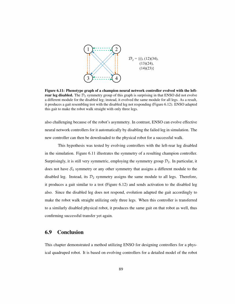
1 2
3 4
= {(), (12)(34), (13)(24), (14)(23)}
D2
Figure 6.11: Phenotype graph of a champion neural network controller evolved with the left-rear leg disabled. The D2 symmetry group of this graph is surprising in that ENSO did not evolvea different module for the disabled leg; instead, it evolved the same module for all legs. As a result,it produces a gait resembling trot with the disabled leg not responding (Figure 6.12). ENSO adaptedthis gait to make the robot walk straight with only three legs.
also challenging because of the robot’s asymmetry. In contrast, ENSO can evolve effective
neural network controllers for it automatically by disabling the failed leg in simulation. The
new controller can then be downloaded to the physical robot for a successful walk.
This hypothesis was tested by evolving controllers with the left-rear leg disabled
in the simulation. Figure 6.11 illustrates the symmetry of a resulting champion controller.
Surprisingly, it is still very symmetric, employing the symmetry group D2. In particular, it
does not have S3 symmetry or any other symmetry that assigns a different module to the
disabled leg. Instead, its D2 symmetry assigns the same module to all legs. Therefore,
it produces a gait similar to a trot (Figure 6.12) and sends activation to the disabled leg
also. Since the disabled leg does not respond, evolution adapted the gait accordingly to
make the robot walk straight utilizing only three legs. When this controller is transferred
to a similarly disabled physical robot, it produces the same gait on that robot as well, thus
confirming successful transfer yet again.
6.9 Conclusion
This chapter demonstrated a method utilizing ENSO for designing controllers for a phys-
ical quadruped robot. It is based on evolving controllers for a detailed model of the robot
89

-240
-180
-120
-60
0
60
120
180
240
0 2 4 6 8 10 12
Leg
Join
t Ang
le (d
eg)
Time (s)
RF LF RR LR
(a) Simulated robot
-240
-180
-120
-60
0
60
120
180
240
0 2 4 6 8 10 12
Leg
Join
t Ang
le (d
eg)
Time (s)
RF LF RR LR
(b) Real robot
Figure 6.12: A gait evolved in simulation with the left-rear leg disabled and transferred to thesimilarly disabled real robot. The plots show the four leg angles of the robot in the first twelveseconds. They were produced by the controller with the phenotype graph illustrated in Figure 6.11.The disabled leg produces a flat line, while the other three legs maintain synchronous and phase-related oscillations resembling a trot gait. However, the synchronous lines for left-front and right-rear legs split slightly from each other between 0° and 180° and the line for the right-front leg curvesa little around 0° indicating adaptation of the gait to produce a straight walk with only three legs.Again, this gait transfers well to the physical robot.
90

in simulation and then transferring the resulting controllers to the physical robot. ENSO’s
symmetry evolution makes this ordinarily challenging transfer process tractable by evolv-
ing symmetric neural network controllers. Since such controllers are actually coupled-cell
systems, they produce stable gaits that are robust to small inaccuracies in the simulation
and uncertainties in the real world. ENSO evolved such effective controllers both for a
fully functional version of the robot and also for its fault-tolerant version with a disabled
leg. Moreover, the results of generalization experiments suggest that they would be robust
to common real-world challenges such as variations in battery performance and obstacles.
91

Chapter 7
Evolving Sorting Networks
Previous chapters demonstrated how the symmetry breaking approach can make evolu-
tionary search more effective in designing controllers for multilegged robots. The same
approach is also potentially useful in other applications with similar modular structure, e.g.
distributed control systems, multiagent systems, and genetic regulatory networks. In other
domains, the alternative process of building a desired symmetry step by step may be a more
appropriate way to constrain search to promising regions. This chapter demonstrates this
idea in one such problem: designing sorting networks with minimal number of compara-
tors. I will begin by representing the network in terms of Boolean functions. I will then
utilize this representation to express the symmetry of the network and thereby develop an
approach for constructing minimal-size networks by building their symmetry in steps.
7.1 Boolean Function Representation
As described in Section 2.4, the zero-one principle can be utilized to express the inputs of
a sorting network as Boolean variables and its outputs as functions of those variables. It
simplifies the sorting problem to counting the number of inputs that have the value 1 and
setting that many of the lowermost outputs to 1 and the remaining outputs to 0. In particular,
92

Figure 7.1: Boolean output functions of a 4-input sorting network. The zero-one principle canbe utilized to represent the inputs of the network as Boolean variables. Each comparator producesthe conjunction of its inputs on its upper line and their disjunction on its lower line. As a result,the functions at the outputs of the network are compositions of conjunctions and disjunctions of theinput variables. In particular, the output function fi at line i is the disjunction of all conjunctiveterms with exactly n + 1 − i variables. Therefore, a sorting network is a sequence of comparatorsthat compute all its output functions from its input variables. This representation makes it possibleto express the symmetry of the network in a way that is suitable for the symmetry-building approach.
the function fi(xi, . . . , xn) at output i takes the value 1 if and only if at least n+1−i inputs
are 1. That is, fi is the disjunction of all conjunctive terms with exactly n+ 1− i variables.
Since these functions are implemented by the comparators in the network, the prob-
lem of designing a sorting network can be restated as the problem of finding a sequence
of comparators that compute its output functions. Each comparator computes the conjunc-
tion (upper line) and disjunction (lower line) of their inputs. As a result, a sequence of
comparators computes Boolean functions that are compositions of conjunctions and dis-
junctions of the input variables (Figure 7.1). Since the number of terms in these functions
can grow exponentially as comparators are added, it is necessary to utilize a representation
that makes it efficient to compute them and to determine whether all output functions have
been computed.
Such functions computed utilizing only conjunctions and disjunctions without any
negations are called monotone Boolean functions (Korshunov, 2003). Such a function f
on n binary variables has the property that f(a) ≤ f(b) for any distinct binary n-tuples
a = a1, . . . , an and b = b1, . . . , bn such that a ≺ b, where a ≺ b if ai ≤ bi for 1 ≤ i ≤ n.
This property makes it possible to represent them efficiently utilizing the Boolean lattice of
binary n-tuples, as illustrated in Figure 7.2 for functions of four variables.
93

1
2
3
4
5 0000
0001 0010
0011
0100
0101 0110
0111
1000
1001 1010
1011
1100
1101 1110
1111
(a) f(x1, x2, x3, x4) = x1
0000
0001 0010
0011
0100
0101 0110
0111
1000
1001 1010
1011
1100
1101 1110
1111
(b) f(x1, x2, x3, x4) = x1 ∨ (x2 ∧ x3)
Figure 7.2: Representation of monotone Boolean functions on four variables in the Booleanlattice. The nodes of the lattice are organized in levels (numbered on the left), each containing thebinary value assignments to the n-tuple x1x2x3x4 with the same number of 1s. Therefore, the truthtable for any Boolean function f(x1, x2, x3, x4) can be represented in this lattice by shading allthe nodes for which f takes the value 1. A node b1b2b3b4 has a path to a lower node a1a2a3a4 ifai ≤ bi for 1 ≤ i ≤ 4. As a result, if node a1a2a3a4 is shaded for a monotone function f , then allhigher nodes reachable from it are also shaded, i.e. f is defined completely by the nodes in the lowerboundary of its shaded region. This set of nodes (shown in bold) corresponds to the conjunctiveterms in the disjunctive normal form of f . For example, it contains just the node 1000 for f = x1
and two nodes 1000 and 0110 for f = x1 ∨ (x2 ∧ x3). This representation makes it possible tocompute such functions efficiently.
94

Any two nodes in this lattice are comparable if they can be ordered by≺. Therefore,
the nodes at which any monotone function f takes the value 1 are bounded at the top by
1111 and bounded below by a set of incomparable nodes (i.e. antichain) corresponding to
the conjunctive terms in its disjunctive normal form, i.e. f is completely specified by the
nodes in its boundary. Moreover, nodes in the same level i (numbered from the top of the
lattice) have the same number n+ 1− i of 1s, forming an antichain of incomparable nodes.
They represent the boundary of the function fi at output i of the sorting network since fi
is the disjunction of all conjunctive terms with exactly n + 1 − i variables (Section 2.4).
Therefore, fi takes the value 1 for all nodes less than or equal to level i and the value 0 for
all nodes greater than level i. This property makes it possible to verify efficiently whether
fi has been computed at output i. Thus, levels 1 to n of the lattice have a one-to-one
correspondence with the output functions of the network.
Since a monotone Boolean function is completely determined by the nodes in its
boundary, only those nodes need to be stored to represent the function. In a lattice of size
2n, the maximum size of this representation is equal to the size of the longest antichain,
which is only(
ndn/2e
)nodes (by Stirling’s approximation,
(ndn/2e
)= O
(2n√
n
)). However,
computing conjunctions and disjunctions utilizing this representation is computationally
expensive and produces a combinatorially large number of redundant, non-boundary nodes
that have to be removed (Gunter et al., 1996). A more efficient representation is storing
the values of the function in its entire truth table as a bit-vector of length 2n. Its values
are grouped according to the levels in its Boolean lattice so that values for any level can be
retrieved easily. This representation also allows computing conjunctions and disjunctions
efficiently as the bitwise AND and OR of the bit-vectors respectively. Moreover, efficient
algorithms for bit-counting make it possible to determine if function fi has been computed
at output i.
This function representation is utilized by the symmetry-building approach to con-
struct minimal-size sorting networks, as will be described next.
95

7.2 Symmetry-Building Approach
Finding a minimum sequence of comparators that computes all output functions of a sort-
ing network through exhaustive search is a challenging combinatorial problem. It can be
made more tractable by utilizing the symmetries of the network, represented in terms of the
symmetries of its set of output functions. This representation of network symmetries makes
it possible to develop a symmetry-building approach for constructing minimal-size sorting
network.
7.2.1 Network Symmetries
Since each output function fi(xi, . . . , xn) is the disjunction of all conjunctive terms with
exactly n + 1 − i variables, it is invariant to all n! permutations of the variables. There-
fore, the ordered set of all output functions fi is itself invariant to all variable permutation,
implying that the network has the symmetries represented by the group Sn.
The network also has symmetries resulting from swapping the outputs of all its
comparators to produce its dual network with the same set of output functions in the re-
verse order. Doing so swaps the conjunctions and disjunctions in the output functions of
the primal network to produce the output functions of the dual network. Using the sym-
bols ∧ and ∨ to specify conjunctions and disjunctions, this duality can be expressed as
fi(xi, . . . , xn,∧,∨) = fn+1−i(xi, . . . , xn,∨,∧) for all 1 ≤ i ≤ n. It is therefore possible
to define symmetry operations σi for 1 ≤ i ≤⌈
n2
⌉that act on the network, swapping the
dual functions fi and fn+1−i and also swapping the conjunctions and disjunctions in them.
Applying these operations on the ordered set of output functions leaves the set invariant.
Their compositions are also symmetries because σi and σj operate independently on differ-
ent pairs of functions, leaving the set of outputs invariant. Therefore, this set of operations
are closed under composition and they are associative. Moreover, each operation is its own
inverse, producing the identity when applied twice in a row. Thus they satisfy all the group
axioms and they therefore produce a group. Since every element of this group can be ex-
96

pressed as the composition of finitely many elements of the set Σ = {σ1, . . . , σdn2 e}, the
group is said to be generated by Σ and it is denoted 〈Σ〉.
The full symmetry group of the network is the combined group of symmetries re-
sulting from permuting the input variables and swapping the conjunctions and disjunctions
in dual output functions. This group is obtained by taking the direct product of Sn and 〈Σ〉,
denoted Sn × 〈Σ〉. Its set of elements is the Cartesian product of its component groups,
i.e. the set of ordered pairs (g, ρ), where g ∈ Sn and ρ ∈ 〈Σ〉. Its group operation is the
component-wise composition, (g, ρ)◦(h, τ) = (g◦h, ρ◦τ). Moreover, two of its subgroups
{(g, e) : g ∈ Sn} and {(e, ρ) : ρ ∈ 〈Σ〉}, where e is the identity, are isomorphic to Sn and
〈Σ〉 respectively, confirming that Sn × 〈Σ〉 contains its component groups.
Therefore, the final symmetry group of the sorting network to be designed is already
known, unlike the multilegged robot controllers in Chapter 5 that required the appropriate
symmetries to be discovered by symmetry breaking. That is, any n-input sorting network
has the symmetry group Sn×〈Σ〉. Such a network can be constructed step by step through a
sequence of subgoals corresponding to the subgroups of this symmetry group, as described
next.
7.2.2 Defining Subgoal Sequence
The subgroups of Sn × 〈Σ〉 represent the symmetries of partial networks created in the
intermediate stages of constructing a sorting network. In particular, computing pairs of dual
output functions produces symmetries corresponding to a subgroup of 〈Σ〉 (Figure 7.3).
Since the elements of Σ operate on different pairs of dual functions, any such subgroup
can be written as 〈Γ〉, where Γ is a subset of Σ. Initially, before any comparators have
been added, each line i in the network has the trivial monotone Boolean function xi. As
a result, the network does not have any symmetries, i.e. Γ = {}. Adding comparators to
compute both the output function fi and its dual fn+1−i yields Γ = {σi} for the resulting
partial network. Adding more comparators to compute both fj and its dual fn+1−j creates
97

a new partial network with Γ = {σi, σj}, i.e. the new partial network is more symmetric.
Continuing to add comparators until all output functions have been constructed produces a
complete sorting network with Γ = Σ.
Thus adding comparators to the network in a particular sequence builds its symme-
try in a corresponding sequence of subgroups 〈Γ〉 that extends from the bottom to the top
of the subgroup lattice of 〈Σ〉. Conversely, building symmetry in a particular sequence con-
strains the possible comparator sequences. Symmetry can therefore be utilized to constrain
the search space for designing networks with desired properties. In particular, the sequence
of subgroups for building symmetry can represent a sequence of subgoals for minimizing
the number of comparators in the network. Each subgoal is defined as the subgroup that
can be produced from the previous subgoal by adding the least number of comparators.
Since Γ = {} initially, the first subgoal is the symmetry that can be produced from
the input variables by adding the least number of comparators (Figure 7.4). Producing this
symmetry in turn requires computing its corresponding dual output functions. Since the
dual functions f1 = x1 ∧ . . .∧xn and fn = x1 ∨ . . .∨xn have the least number of variable
combinations, they can be computed by adding fewer comparators than any other pair of
dual output functions. Therefore, the first subgoal is to produce the symmetry Γ = {σ1} by
adding the least number of comparators.
After computing f1 and fn, the next pair of dual output functions with the least
number of variable combinations are f2 and fn−1. Therefore, they are likely to be the next
pair of dual functions that require the least number of comparators to compute, making
the symmetry Γ = {σ1, σ2} the next subgoal. The number of variable combinations in
the output functions continues to increase from the outer lines to the middle lines of the
network. Therefore, from any subgoal that adds the symmetry σk to Γ, the next subgoal
adds the symmetry σk+1 to Γ. This sequence of subgoals continues until all the output
functions are computed, producing the final goal symmetry Γ = {σ1, . . . , σdn2 e}. The
98

Figure 7.3: Symmetries of output function duals in 4-input sorting networks. The numberbelow each comparator indicates the sequence in which it is added to construct the network. Thelast comparator touching horizontal line i completes computing the output function fi for that line.Functions fi and fn+1−i form a dual, and computing them both gives the network the symmetry σi.In network (a), comparator 3 completes computing f1 and when comparator 4 completes computingits dual f4, the network gets the symmetry σ1. Comparator 5 then completes computing both f2and its dual f3, giving the network another symmetry σ2. Network (b) also produces the samesequence of symmetries and has the same number of comparators. In network (c), comparator5 completes computing both f3 and f4. However, it gets the symmetries σ1 and σ2 only whencomparator 6 completes computing their duals f1 and f2. Network (d) is similar, and they bothrequire one more comparator than networks (a) and (b). Thus the goal set of symmetries for a 4-input network is Γ = {σ1, σ2}, i.e. it is already known. Building this set of symmetries step bystep corresponds to constructing such a network by adding comparators, some symmetry sequencesrequiring longer comparator sequences. Therefore, constructing the network in this manner througha suitable sequence of symmetries can be utilized to minimize its comparator requirement.
99

Figure 7.4: Subgoals for constructing a 4-input sorting network with minimum number ofcomparators. The final goal is to produce the symmetry group 〈Γ〉, where Γ = {σ1, σ2}, bycomputing all four output functions fi with the minimum number of comparators. This goal canbe decomposed into a sequence of subgoals specified as subgroups of the final symmetry group. Atany stage in the construction, the next subgoal is the subgroup that can be produced by adding theleast number of comparators. Initially, the network does not have any symmetries, i.e. Γ = {}. Thedual functions f1 and f4 require fewer comparators than f2 and f3 to compute because they havefewer combinations of the input variables. Therefore, the first subgoal is to produce the symmetryΓ = {σ1}. In order to reach this subgoal with the minimum number of comparators, the samecomparators 1 and 2 compute parts of both f1 and f4. The second and final subgoal is to producethe symmetry Γ = {σ1, σ2}. The functions f2 and f3 that produce that symmetry have already beenpartially computed by comparators 3 and 4. Therefore, adding comparator 5 completes computingboth f2 and f3. In this way, the number of comparators required to reach each subgoal can beoptimized separately, making it tractable to search for minimum-size sorting networks with a largenumber of inputs.
100

number of comparators required to reach each of these subgoals is minimized as described
next.
7.2.3 Minimizing Comparator Requirement
In order to reach the first subgoal, the same comparator can compute a conjunction for f1
and also a disjunction for fn simultaneously (Figure 7.4). Sharing the same comparator to
compute dual functions in this manner reduces the number of comparators required in the
network. However, such sharing between dual functions of the same subgoal is possible
only in some cases. In other cases, it may still be possible to share a comparator with the
dual function of a later subgoal. Constructing minimal-size sorting networks requires deter-
mining which comparators can be shared and then adding those comparators that maximize
sharing.
The Boolean lattice representation of functions discussed in Section 7.1 can be uti-
lized to determine whether sharing a comparator by computing parts of two functions si-
multaneously is possible (Figure 7.5). Assume that the current subgoal requires computing
the output function fi and its dual fn+1−i. That is, functions for outputs less than i and
greater than n + 1 − i have already been computed. All the remaining output functions
will need to have the value 1 for all nodes in levels less than or equal to i and the value
0 for all nodes in levels greater than n + 1 − i. Therefore, the current functions on lines
i ≤ j ≤ n+ 1− i are also guaranteed to have the same values for those levels. Otherwise,
computing at least one of the output functions by adding comparators will be impossible
(since conjunctions preserve 0s and disjunctions preserve 1s).
For the current subgoal, function fi can be computed by setting its value for all
nodes in level i to 1 and all nodes in level i+ 1 to 0, thus defining its node boundary in the
lattice. Its monotonicity then implies that its value for all nodes in levels less than i will
be set to 1 automatically and its value at all nodes in levels greater than i + 1 will be set
to 0 automatically. However, since fi is computed from the current functions f ′j on lines
101

1
2
3
4
5 0000
0001 0010
0011
0100
0101 0110
0111
1000
1001 1010
1011
1100
1101 1110
1111
(a) x1
0000
0001 0010
0011
0100
0101 0110
0111
1000
1001 1010
1011
1100
1101 1110
1111
(b) x2
1
2
3
4
5 0000
0001 0010
0011
0100
0101 0110
0111
1000
1001 1010
1011
1100
1101 1110
1111
(c) x1 ∧ x2
0000
0001 0010
0011
0100
0101 0110
0111
1000
1001 1010
1011
1100
1101 1110
1111
(d) x1 ∨ x2
Figure 7.5: Comparator sharing to compute dual output functions in a 4-input sorting net-work. This figure illustrates the Boolean lattice representation of the functions computed by com-parator 1 in Figure 7.4. The levels of the lattices are numbered on the left and the nodes for which thefunction value is 1 are shaded. Comparator 1 computes the conjunction (c) and the disjunction (d)of the functions (a) and (b) for the subgoal of computing the output functions f1 = x1∧x2∧x3∧x4
and f4 = x1 ∨ x2 ∨ x3 ∨ x4. Function f1 can be computed by utilizing conjunctions to set the valuefor all nodes in level 2 of the lattice to 0. Similarly, f4 can be computed by utilizing disjunctionsto set the value for all nodes in level 4 to 1. Therefore, comparator 1 contributes to computing bothf1 and f4 by setting the values of two nodes in level 2 of its conjunction to 0 and the values of twonodes in level 4 of its disjunction to 1. Such shared computation reduces the number of comparatorsrequired to construct sorting networks.
102

i ≤ j ≤ n+ 1− i and they already have the value 1 for all nodes in levels less than or equal
to i, the function fi will also get the same value for those nodes automatically. Therefore,
fi can be computed just by setting the values for all nodes in level i+ 1 to 0.
The value for a particular node is set to 0 by utilizing a comparator that computes its
conjunction with another function that already has the value 0 for that node. Moreover, the
disjunction that the comparator also computes has the value 1 for all nodes in level i+ 1 as
required for the other output functions that are yet to be computed. Therefore, exactly one
of the functions f ′j already has the value 0 for any particular node in level i + 1. Adding a
comparator between a pair of such functions computes their conjunction with the 0-valued
nodes from both functions. Repeating this process recursively collects the 0-valued nodes
in level i + 1 from all functions to the function on line i, thus producing fi. Similarly, its
dual function fn+1−i can also be computed from the functions f ′j by utilizing disjunctions
instead of conjunctions to set its values for all nodes in level n+ 1− i to 1.
The leaves of the resulting binary recursion tree for fi are the functions f ′j that have
0-valued nodes in level i + 1 and its internal nodes are the comparators. Since the number
of nodes of degree 2 in a binary tree is one less than the number of leaves (Mehta and Sahni,
2005), the number of comparators required depends only on the number of functions the
recursion starts with, i.e. it is invariant to the order in which the recursion pairs the leaves.
However, the recursion trees for fi and fn+1−i may have common leaves, making it possible
to utilize the same comparator to compute a conjunction for fi and a disjunction for fn+1−i.
Maximizing such sharing of comparators between the two recursion trees minimizes the
number of comparators required for the current subgoal.
It may also be possible to share a comparator with a later subgoal, e.g. when it
computes a conjunction for fi and a disjunction for fn+1−k, where i < k ≤⌈
n2
⌉. In order
to prioritize subgoals and determine which comparators maximize sharing, each pair of
lines where a comparator can potentially be added is assigned a utility. Comparators that
contribute to both fi and fn+1−i for the current subgoal get the highest utility. Comparators
103

that contribute to an output function for the current subgoal and an output function for the
next subgoal get the next highest utility. Similarly, other possible comparators are also
assigned utilities based on the output functions to which they contribute and the subgoals to
which those output functions belong. Many comparators may have the same highest utility;
therefore, one comparator is chosen randomly from that set and it is added to the network.
Repeating this process produces a sequence of comparators that optimizes sharing within
the current subgoal and between the current subgoal and later subgoals.
7.3 Evolving Minimal-Size Networks
Optimizing for each subgoal separately in the above manner constitutes a greedy algorithm
that produces minimal-size networks with high probability for n ≤ 8. However, for larger
values of n, the number of subgoals is too many to find a global optimum reliably. In such
cases, its performance can be improved by utilizing evolution to optimize the solutions
further.
The most straightforward approach is to initialize evolution with a population of so-
lutions that the greedy algorithm produces. The fitness of each solution is the negative of its
number of comparators so that improving fitness will minimize the number of comparators.
In each generation, two-way tournament selection based on this fitness measure is utilized
to select the best individuals in the population for reproduction. Reproduction mutates the
parent network, creating an offspring network in two steps: (1) a comparator is chosen from
the network randomly to truncate the network, discarding all comparators that were added
after it, and (2) the greedy algorithm is utilized to add comparators again, reconstructing a
new offspring network. Since the greedy algorithm chooses a comparator with the highest
utility randomly, this mutation explores a new combination of comparators that might be
more optimal than the parent.
This straightforward approach restricts the search to the space of comparator com-
binations suggested by the greedy algorithm and assumes that it contains a globally minimal
104

network. But in some cases, the globally minimal networks may utilize comparators that
are different from those suggested by the greedy algorithm. Therefore, a more powerful
(but still brute force) approach is to let evolution utilize such comparators as well: With a
low probability, the suggestions of the greedy algorithm are ignored and instead the next
comparator to be added to the network is selected randomly from the set of all potential
comparators.
A more effective way to combine evolution with such departures from the greedy
algorithm is to utilize an Estimation of Distribution Algorithm (EDA) (Alden, 2007, Ben-
goetxea et al., 2001, Muhlenbein and Hons, 2005). The idea is to estimate the probability
distribution of optimal comparator combinations and to utilize this distribution to generate
comparator suggestions. The EDA is initialized as before with a population of networks
generated by the greedy algorithm. In each generation, a set of networks with the highest
fitness are selected from the population. These networks are utilized in three ways: (1) to
estimate the distribution of optimal comparators for a generative model, (2) as elite net-
works passed unmodified to the next generation, and (3) as parent networks from which
new offspring networks are created for the next generation.
The generative model of the EDA specifies the probability P (C|S) of adding a
comparator C to an n-input partial network with state S. The state of a partial network is
defined in terms of the n Boolean functions that its comparators compute. These functions
determine the remaining comparators that are needed to finish computing the output func-
tions, making them a good representation of the partial network. However, storing the state
as the concatenation of the n functions is computationally intractable since each function is
represented as a vector of 2n bits. Therefore, a condensed state representation is computed
based on the observation that the greedy algorithm does not utilize the actual function val-
ues for the nodes in the Boolean lattice; it only checks whether the values in a given level
are all 0s or all 1s. This information, encoded as 2(n + 1) bits (Figure 7.6), is suitable as
the state representation for the model as well.
105

0000
0001 0010
0011
0100
0101 0110
0111
1000
1001 1010
1011
1100
1101 1110
1111 01
00
00
10
10
Figure 7.6: State representation of the function x1∧x2 utilized in the EDA. The state (shown onthe right) is a bit-string with two bits for each level of the Boolean lattice. The first bit is 1 only if thevalue of the function for all nodes in that level is 0 and the second bit is 1 only if its value for all nodesin that level is 1. This condensed representation of the function is based on the information utilizedby the symmetry-building greedy algorithm and it is therefore useful for constructing minimal-sizesorting networks.
Since the model is estimated from the set of the smallest networks in the population,
it is likely to generate small networks as well. Although it can generate new networks
from scratch, it is utilized as part of the above reproduction mechanism to reconstruct a
new offspring network from the truncated parent network, i.e. it is utilized in step 2 of
reproduction instead of the greedy algorithm. In this step, some comparators are also chosen
randomly from the set of all potential comparators to encourage exploration of comparator
combinations outside the model. Moreover, if the model does not generate any comparators
for the current state, then the greedy algorithm is utilized to add a comparator. The resulting
EDA finds smaller sorting networks than previous results, as demonstrated next.
7.4 Results
The EDA was run with a population size of 200 for 500 generations to evolve minimal-
size networks for different input sizes. In each generation, the top half of the population
(i.e. 100 networks with the least number of comparators) was selected for estimating the
model. The same set of networks was copied to the next generation without modification.
106

Each of them also reproduced an offspring network to replace those in the bottom half of
the population. A Gaussian probability distribution was utilized to select the comparator
from which to truncate the parent network. The Gaussian was centered at the middle of its
comparator sequence with a standard deviation of one-fourth its number of comparators. As
a result, parent networks are more likely to be truncated near the middle than near the ends.
When reconstructing the truncated network, the next comparator to add to the network is
generated either by the estimated model (with probability 0.5) or is selected randomly from
the set of all potential comparators (with probability 0.5).
The above experiments (variant 1) were repeated with a slight modification of the
greedy algorithm used to initialize the population for the EDA. If the set of compara-
tors with the highest utility contains a comparator that is symmetric with respect to an-
other comparator already in the network, then it prefers that comparator (Graham and Op-
pacher, 2006). This modification (variant 2) makes the arrangement of comparators in
the network more bilaterally symmetric about a horizontal axis through the middle of the
network. Biasing the networks with this type of symmetry produced smaller networks
for some input sizes. The source code for both variants is available from the website
http://nn.cs.utexas.edu/?sorting-code.
Both variants were run 20 times, each time with a different random number seed.
The least number of comparators that they found for each input size is listed in Table 7.1.
For input sizes n ≤ 11, the initial population of the EDA already contained networks with
the smallest-known sizes for all 20 runs, i.e. the greedy algorithm was sufficient to find the
smallest-known networks. As discussed in Section 3.3, optimality of such networks has
been proven only for n ≤ 8. For input sizes 12, 13, 14, 16, 21, and 23, the EDA evolved
networks that have the same size as the best known networks. Moreover, it improved the
previous best results for input sizes 17, 18, 19, 20, and 22 by one or two comparators.
Examples of these networks are listed in Appendix A. Prospects of extending to n > 24
will be discussed in Chapter 8.
107

n 12 13 14 15 16 17 18 19 20 21 22 23 24
Previous bestHand-design and END Batcher’s merge on smaller networks39 45 51 56 60 73 80 88 93 103 110 118 123
EDA 39 45 51 57 60 71 78 86 92 103 108 118 125
Table 7.1: Sizes of the smallest networks for different input sizes found by the EDA. For inputsizes n ≤ 11, networks with the smallest-known sizes (Section 3.3) were already found in the initialpopulation of the EDA, i.e. the greedy algorithm was sufficient. These sizes are therefore omittedfrom this table. For larger input sizes, evolution found networks that matched previous best results(indicated in italics) or improved them (indicated in bold). Appendix A lists examples of thesenetworks. EDA variant 2 produced better results than variant 1 for input sizes 15, 17, 18, 20, 22,23, and 24. Prospects of extending these results to input sizes greater than 24 will be discussedin Chapter 8. These results demonstrate that the symmetry-based EDA approach is effective atdesigning minimal-size sorting networks and has advanced the state-of-the-art.
The previous best results were obtained either by hand design or by the END evolu-
tionary algorithm (Baddar, 2009, Juille, 1995, Knuth, 1998). The END algorithm improved
a 25-year old result for the 13-input case by one comparator and matched the best known
results for other input sizes up to 16. However, it is a massively parallel search algorithm,
requiring very large computational resources, e.g. it required a population size of 65,536
on 4096 processors to find minimal-size networks for 13 and 16 inputs. In contrast, the
symmetry-based EDA algorithm finds such networks with much smaller resources (e.g.
population size of 200 on a single processor in a similar number of generations), making it
computationally feasible to solve larger problems.
7.5 Conclusion
Minimizing the number of comparators in a sorting network is a challenging optimization
problem. This chapter presented an approach that converts it into the problem of building
the symmetry of the network optimally. The resulting problem structure makes it possible
to construct the network in steps and to minimize the number of comparators required for
each step separately. This approach produces greedy solutions that are optimized further
by evolution, exploring the neighborhood of these solutions in more detail. As with ENSO,
108

the resulting algorithm focuses search on promising regions of the search space, making it
possible to find minimal-size networks efficiently. For several input sizes, these networks
are smaller than the previous best results, thus advancing the state-of-the-art for designing
minimal-size sorting networks.
109

Chapter 8
Discussion and Future Work
The work presented in previous chapters explored the hypothesis that symmetry can be
utilized to constrain the design space meaningfully, making it possible to solve challenging
engineering problems. For multilegged robots walking on flat ground, it was possible to
constrain the controllers to a single hand-designed symmetry and evolve only the remaining
parameters. Since it is not always possible to hand-design the appropriate symmetries,
the ENSO approach was developed to evolve them automatically. ENSO utilizes group
theory to break symmetry systematically, thereby constraining search to the most promising
symmetries. The alternative process of building symmetry systematically was also useful
in constraining the search space for finding minimal-size sorting networks. This chapter
evaluates these results, discusses the insights gained from them, and proposes directions for
future work.
8.1 Hand-Designed Symmetries
Modular neuroevolution with hand-designed symmetries produced controllers that were
better than those produced by non-modular evolution with no symmetries in two respects:
(1) they achieved a better fitness by travelling farther, and (2) they employed better gaits
110

that were symmetric, resembling those found in nature. Furthermore, this performance
gap widened significantly in both respects when the number of legs or their degrees of
freedom were increased. The symmetric controllers also demonstrated the capability to
change gaits in response to changes in the environment. Changing gaits on an obstacle
terrain made it easier for the robot to negotiate bumps. These results suggest that utilizing
symmetries to constrain the search space makes it possible for modular neuroevolution to
discover effective controllers.
In these experiments, the controllers were always evaluated by starting the robot
from the same position. As a result, some evolved behaviors such as changing gaits to
negotiate obstacles are not robust to different starting positions. They can be made more
robust by averaging evaluations over multiple random starting positions or by adding noise
to the simulation during evaluations as was done for the physical robot. Utilizing sensors
that provide feedback about the environment may also improve robustness.
The controller symmetries were designed analytically using the theory of coupled
cell systems. Hand-designing symmetries in this manner is too restrictive in the general case
for two reasons. First, in the special case it was possible to replicate a single module for each
leg because the legs were identical. In a more complex robot, more than one type of module
may be needed, for example to control different types of front and rear legs. The resulting
coupled cell system will have more than one type of cell and therefore different symmetries.
Second, in the special case the coupling between the cells and the assignment of cells to legs
was also determined by the hand-designed symmetries. More sophisticated behaviors may
require different cell couplings and assignments that utilize different symmetries to explore
a different part of the search space. Although hand-designing symmetries is possible in
simple cases, it cannot (at least not as easily) be done in such complex, real-world cases.
Therefore, it is useful to evolve the appropriate symmetries automatically. However,
the results of non-modular evolution suggests that it is too difficult to evolve symmetries
in the unconstrained space of all possible symmetries. Consequently, a more constrained
111

approach that makes it possible to explore the space of symmetries in a meaningful way is
necessary. The ENSO approach accomplishes this goal.
8.2 Symmetry Evolution with ENSO
Given the number of modules, ENSO’s group-theory-based systematic symmetry search
makes it possible to evolve the appropriate symmetry automatically. Demonstrating this
capability, ENSO evolved gaits similar to those based on hand-designed symmetries on flat
ground, and significantly faster gaits on inclined ground, for a quadruped robot. These gaits
also generalized better when friction was reduced to make the ground slippery. As in the
previous experiments with hand-designed symmetries, these gaits were evolved by starting
the robot from the same position and orientation on the incline in every evaluation. More
robust gaits can potentially be evolved by randomizing the initial orientation, by sensing
the slope of the incline, or by adding noise to the simulation. Such robust gaits were indeed
evolved for the physical robot in Chapter 6.
In order to verify that ENSO’s symmetry-breaking approach is indeed a useful way
to constrain search, it was compared with the less principled, random-symmetry-evolution
approach. Random-symmetry evolution produces significantly worse gaits than ENSO be-
cause its unsystematic symmetry mutations often result in large changes in symmetry. In
contrast, the group-theoretic mutations of ENSO result in only minimal changes in sym-
metry, making complexification possible (Section 2.1): Evolution starts with a highly sym-
metric (i.e. simple) controller and breaks the symmetry incrementally, producing gradual
increases in complexity. As a result, evolution optimizes simpler controllers before elabo-
rating on these by adding more parameters. Thus the complexification resulting from sym-
metry breaking provides ENSO with a smoother fitness gradient, making evolution easier.
In addition to these evolutionary advantages that group theory provides, the theory
of coupled cell systems provides ENSO with guarantees on the behavior of evolved con-
trollers. For example, if the symmetries of a coupled cell system admit a particular gait,
112

then there exists an instance of the system with an asymptotically stable periodic solution
(i.e. limit cycle) implementing that gait (Golubitsky and Stewart, 2002). As a result, the gait
is robust to small perturbations. ENSO constrains neuroevolution to find such an instance
of the control system. When the dynamics of this system was perturbed manually (utiliz-
ing a visualization interface to the physical simulation) the gaits they generate were indeed
found to be robust. Such robustness is useful in controllers of real-world robots because
their interactions with environment are frequently perturbed.
As discussed in Section 2.3, the symmetries of coupled cell systems also makes
it possible for the same controller to produce multiple gaits. Each gait is a stable limit
cycle of the coupled cell system, and the system can transition from one limit cycle to
another when perturbed. Sometimes small perturbations, caused by physical interaction
with the environment, can trigger such a transition. Figure 5.5d shows an example of this
phenomenon, where the robot changes from an initial pronk to a trot at about three seconds
into the simulation. If the robot is prevented from interacting with the ground, then this
change does not occur and the robot continues executing the pronk gait. The ability of
controllers to generate such different gaits makes it possible to use the most effective gait
for a given terrain, including those that allow it to go over obstacles (Section 4.7).
It is difficult to obtain the above properties in controllers evolved without such math-
ematical models. For example, oscillations required for generating gaits needed to be sup-
plied as external inputs to quadruped controllers evolved using the HyperNEAT method
(Clune et al., 2009). These properties were crucial in transferring the controllers that ENSO
evolved in simulation to a physical robot.
These results suggest that ENSO is an effective approach for evolving locomotion
controllers for multilegged robots. In the future, ENSO should be tested with more complex
robots with more legs, more complex legs, and sensors that receive more varied stimuli from
the environment. Their controllers can be modeled as coupled cell systems with more cells
and cells receiving additional inputs. Utilizing such more sophisticated models should make
113

it possible for ENSO to evolve controllers that produce high-level behaviors such as path-
following and foraging, in addition to generating regular gaits. ENSO is thus a promising
approach for developing efficient, robust, and flexible controllers for multilegged robots in
the real world.
ENSO breaks symmetry by utilizing the prior knowledge encoded in the subgroup
lattice. In contrast, symmetry-breaking occurs spontaneously in nature when perturbations
induce a physical system in a symmetric (but unstable) state to transition to a less symmetric
(but stable) state with lower energy (Brading and Castellani, 2008, Kovacs, 1986). That is,
the dynamics of natural phenomena encode the knowledge in the subgroup lattice implicitly.
Nature can therefore utilize these phenomena to break symmetry in biological evolution.
Whether modeling them in artificial evolution is an effective substitute for the constraints
encoded explicitly in the subgroup lattice is an interesting question for future research.
8.3 Evolving Controllers for a Physical Robot
ENSO evolved controllers that produced the same gaits in the physical robot as they did in
simulation. Moreover, these gaits were robust to uncertainties that commonly occur in the
real world such as changes in ground friction between different surfaces, initial positions of
legs from which the robot starts walking, and the maximum angular velocity that the motors
can produce. The transfer was successful because of two factors: (1) ENSO was able to
evolve robust controllers that produce stable gaits, and (2) it was possible to simulate the
physical characteristics of the robot with sufficient accuracy.
It is often difficult to transfer controllers evolved in simulation to the real world
because it is difficult to simulate the physical robot and its environment accurately (Gomez
and Miikkulainen, 2004, Lipson et al., 2006). However, this requirement is less critical
for the controllers that ENSO evolves because their robustness can compensate for small
deviations from ideal behavior. For example, instead of detailed mesh models of the robot
morphology, only a crude approximation of its weight distribution was required. Moreover,
114

it turned out sufficient to model the idiosyncratic properties of the motors and uncertainties
in their behavior using interpolation and noise.
Evolving controllers in simulation and then transferring them to the real robot in
this manner is an effective alternative to designing controllers by hand. Hand-design is
difficult because it requires anticipating all possible operating conditions. Moreover, this
laborious process has to be repeated whenever the configuration of the robot changes and it
may even be impossible in some cases. In contrast, evolution can design a new controller
automatically for the new configuration in simulation. For example, if a leg actuator fails
on a quadruped robot during a remote mission, then it must continue the mission with min-
imum performance degradation by utilizing only the remaining three legs. ENSO evolved
a straight and effective gait for such a three-legged configuration by disabling a leg in sim-
ulation. The resulting controller produced the same gait when transferred to the physical
robot as well, suggesting that ENSO’s symmetry-based approach can be utilized to design
fault-tolerant robots for real-world applications.
The physical quadruped robot can be extended to a hexapod easily by adding two
more legs to attachments in the middle. This extension should be able to demonstrate that
the ENSO approach scales up for a physical robot with more legs. ENSO can also be tested
on a robot with more complex legs by designing new legs with additional joints. Another
interesting way to extend the robot is to attach Dynamixel AX-S1 sensors to measure dis-
tance Robotis (2010). Readings from these sensors can then be used as additional controller
inputs, making it possible to evolve behaviors that respond effectively to obstacles in the
environment. Such extensions can build up the sophistication necessary for real-world ap-
plications.
8.4 Utilizing Domain Knowledge in ENSO
ENSO can also evolve controllers for robots with more legs and more degrees of freedom
per leg, such as those discussed in Chapter 4. These robots may have more joints per leg
115

such as a knee joint in addition to the hip joint. The controllers for such robots may need a
different module for each type of joint. Moreover, the knee joint of one leg is not likely to
influence the hip joint of another leg directly, allowing this domain knowledge to be used to
restrict the connectivity of the graphs in the initial population of ENSO. In particular, each
knee module is connected only to the hip module of the same leg, while the hip modules
of all legs are fully interconnected as before. Utilizing domain knowledge in this manner
to constrain the space of symmetries makes it easier for evolution to optimize the resulting
controller.
The above robot morphology can be extended further by adding a foot joint to each
leg, resulting in a controller with local interconnections between the hip, knee and foot
modules. However, it is more convenient to represent such controllers using a two-level
hierarchy instead of using a flat structure. The top level of the hierarchy contains the in-
terconnection structure between leg modules. Each leg module is then decomposed into a
second level, containing the interconnection structure between the hip, knee and foot mod-
ules for that leg. Such a hierarchical phenotype graph can be encoded by a hierarchical
genotype tree (Figure 8.1). The vertex color in the top-level tree contains a special param-
eter that is a pointer to the bottom-level genotype tree. This hierarchical genotype allows
the phenotype structure of each level to evolve independently. Moreover, it decomposes
the phenotype graph into smaller graphs, whose symmetries can be evolved more easily
because their automorphism groups are smaller.
Future experiments along these lines should demonstrate that (1) domain knowledge
can be effectively incorporated into the ENSO approach by constraining the initial struc-
ture of the phenotype graph, and (2) the ENSO approach can design complex controller
networks consisting of different modules and interconnection structures by evolving them
together. These capabilities may be necessary to design controllers for complex robots, e.g.
amphibious robots that can swim in water and walk on land, robotic manipulators that con-
116

PhenotypeGenotype
5 6
7
5 6
7
5 6
7
5 6
7
1 2
3 4
V x V:Params:
1111111111111111
p1,...,pk q1...,qm
Nil
Params: Params:Edges: 0111101111101110Vertices:1000010000100001
V x V:Params:
111111111
p1,...,pk q1...,qm
Nil
Params: Params:Edges: 011101110Vertices:100010001
Figure 8.1: A two-level hierarchical genotype and phenotype. Modules of the top-level of thephenotype graph are decomposed into smaller interconnected modules, creating the bottom-levelphenotype graphs. In the top-level of the corresponding genotype tree, the vertex color contains aspecial parameter that stores the genotype tree for the bottom-level phenotype graph. Decomposingthe phenotype graph into smaller graphs in this manner should make it easier to evolve its symmetry,and constitutes an interesting direction of future work.
sist of several parts for use in industrial applications, and serpentine robots that move by
flexing their spine.
8.5 Other Applications of ENSO
ENSO can also be used to evolve solutions for other control problems that are characterized
by symmetry and modularity. For example, it can be used to design multiagent systems
consisting of agents that interact with each other and with the environment, like those in
online auctions and in robotic soccer (Stone and Veloso, 2000). The behavior of these
agents can be represented as neural network modules and their interactions as (symmetric)
connections between the modules. Another application is in designing distributed control
systems for automated manufacturing processes (McFarlane, 1998). Such systems consist
of controller modules interconnected by communication networks and they can therefore
be implemented as modular neural networks. In both cases, identical modules and connec-
tions between them produce symmetries that ENSO can evolve to design effective control
117

systems. Similarly, ENSO can be used to design distributed computing systems such as a
computer network of clients and servers by evolving the parameters and topology of those
networks (Berryman et al., 2004).
Besides controllers for multilegged locomotion, coupled cell systems can also model
other dynamical systems in nature as symmetric networks. As a result, ENSO can poten-
tially be used to optimize them. For example, coupled cell systems have been used to study
the formation of new species in nature (Golubitsky and Stewart, 2002), the role of structural
symmetries of the visual cortex in inducing visual hallucinations (Golubitsky et al., 2003),
and the properties of genetic regulatory networks (Edwards and Glass, 2000). ENSO can
be used as a tool both for understanding such biological phenomena and for engineering
artificial systems based on them.
8.6 Extending ENSO
Some of the above applications may require extending ENSO in various ways to improve its
capabilities. First, modules with a fixed neural network architecture (i.e. network topology)
was sufficient for the multilegged robot controllers that ENSO evolved in this dissertation.
However, more complex applications may require more complex topologies. In such ap-
plications, ENSO can evolve the topology of the modules by utilizing techniques such as
NEAT (Stanley and Miikkulainen, 2004).
Second, in many applications such as distributed controllers and multiagent sys-
tems, the number of modules remains fixed and is known. ENSO requires the user to
specify this domain knowledge, making it possible to initialize evolution with the appropri-
ate most general symmetries. However, in other applications such as biological networks
(Kepes, 2007) and body-brain evolution (Bongard and Pfeifer, 2003), the modules may not
be known a priori. If the number of modules is constant as in biological networks, then
ENSO can potentially be extended with clustering algorithms to determine the modules au-
118

tomatically (Gao et al., 2009). If the number of modules changes as in body-brain evolution,
then ENSO will have to change the subgroup lattice accordingly.
Third, crossover of genotypes to produce offspring is useful in applications that
benefit from the building-block hypothesis: In such applications, it is possible to assem-
ble functionally complementary blocks from different parents (Watson and Jansen, 2007).
Therefore, in addition to the mutation operators that ENSO already implements, it should
be extended to include crossover, e.g. by swapping subtrees that have the same structure and
node colors. Such subtrees preserve symmetries in the offspring and are therefore likely to
have similar roles in their parents, making crossover effective.
Fourth, although only the leaf nodes of the genotype trees represent the phenotype
graph in the current implementation, an even more compact representation is possible. The
child nodes could inherit one or more parameter values from their parent instead of speci-
fying those parameter values repeatedly in each child node. This feature is useful for rep-
resenting variations of similar elements compactly, which is a common theme in complex
systems with regularities (Stanley, 2007, Stanley and Miikkulainen, 2003). Such elements
can be constructed from leaf nodes that inherit some parameters from a common parent, but
specify different values for other parameters in the leaf nodes. As a result, these elements
have the same values for parameters inherited from the parent, while they differ in the val-
ues for parameters specified in the leaf nodes, i.e. they represent variations on a common
theme such an extension would allow.
Fifth, ENSO utilizes the computational group theory functions of GAP (2007) to
compute the subgroup lattice required for breaking symmetry. However, computing the
subgroup lattice is combinatorially hard in the number of graph vertices. For evolving
larger graphs, ENSO’s scalability can be improved by approximating its group theory com-
putations with fast graph computations. In particular, the orbital partitions of subgroups can
be approximated with 2-stable colorings (Bastert, 2001). For a graph with vertex set v, this
approximation will allow ENSO to search directly in the partition lattice of V × V instead
119

of in the subgroup lattice of S|V |, thus avoiding the computation of the subgroup lattice
at the cost of visiting more points on the partition lattice. However, this additional cost is
likely to be small because the stabilization algorithms used to compute 2-stable colorings
produce orbital partitions in many favorable cases (Bastert, 2001).
These extensions would improve evolutionary search, potentially making it possible
for ENSO to solve more difficult problems and a wider variety of problems.
8.7 Evolving Sorting Networks
The general principle on which ENSO is based, i.e. constraining search by utilizing sym-
metry, is broadly applicable, as demonstrated by evolving minimal-size sorting networks.
Previous results on designing such networks automatically by search have been limited to
small input sizes (n ≤ 16) because the number of valid sorting networks near the opti-
mal size is very small compared to the combinatorially large space that has to be searched
(Juille, 1995). The symmetry-building approach presented in Chapter 7 mitigates this prob-
lem by utilizing symmetry to focus the search on the space of networks near the optimal
size. As a result, it was possible to search for minimal-size networks with more inputs
(n ≤ 24), improving the previous best results in five cases.
It should be possible to improve these results further and to scale them to larger
values of n by extending this symmetry-based approach in the following ways. First, the
greedy algorithm for adding comparators can be improved by evaluating the sharing utility
of groups of one or more comparators instead of single comparators. Such groups having
the highest average utility will then be preferred.
Second, the greedy algorithm can be made less greedy by considering the impact
of current comparator choices on the number of comparators that will be required for later
subgoals. This analysis will make it possible to optimize across subgoals, potentially pro-
ducing smaller networks at the cost of additional computations.
120

Third, the state representation that the EDA algorithm utilizes contains only sparse
information about the functions computed by the comparators. Extending it to include
more relevant information should make it possible for the EDA to disambiguate overlapping
states and therefore to model comparator distribution more accurately.
Fourth, the EDA generates comparators to add to the network only if the state of the
network matches a state in the generative model exactly. Making this match fuzzy based
on some similarity measure may produce better results by exploring similar states when an
exact match is not found.
Fifth, evolutionary search can be parallelized, e.g. using the massively parallel END
algorithm that has been shown to evolve the best known network sizes for n ≤ 16 (Juille,
1995). Utilizing the symmetry-building approach to constrain the search space should make
it possible to run the END algorithm on networks with more inputs.
Sixth, the symmetry-building approach itself can be improved. For example, it
utilizes only the symmetries resulting from the duality of the output functions. It may
be possible to extend this approach by also utilizing the symmetries resulting from the
permutations of the input variables.
Seventh, large networks can be constructed from smaller networks by merging the
outputs of the smaller networks. Since smaller networks are easier to optimize, they can
be evolved first and then merged by continuing evolution to add more comparators. This
construction is similar to utilizing the odd-even merge (Batcher, 1968) to construct minimal
networks for n > 16 from smaller networks.
In addition to finding minimal-size networks, the same symmetry-based approach
can also be utilized to find minimal-delay networks. Instead of minimizing the number of
comparators, it would now minimize the number of parallel steps into which the compara-
tors are grouped. Both these objectives can be optimized simultaneously as well, either
by preferring one objective over the other in the fitness function or by utilizing a multi-
objective optimization algorithm such as NSGA-II (Deb et al., 2000).
121

Moreover, this approach can potentially be extended to design comparator networks
for other related problems such as rank order filters (Chakrabarti and Wang, 1994, Chung
and Lin, 1997, Hiasat and Hasan, 2003). A rank order filter with rank r selects the rth
largest element from an input set of n elements. Such filters are widely used in image
and signal processing applications, e.g. to reduce high-frequency noise while preserving
edge information. Since these filters are often implemented in hardware, minimizing their
comparator requirement is necessary to minimize their chip area. More generally, similar
symmetry-based approaches may be useful for designing stack filters, i.e. circuits imple-
menting monotone Boolean functions, which are also popular in signal processing appli-
cations (Hiasat and Hasan, 2003, Shmulevich et al., 1995). Furthermore, such approaches
can potentially be used to design rearrangeable networks for switching applications as well
(Seo et al., 1993, Yeh and Feng, 1992).
8.8 Conclusion
Utilizing symmetries to constrain evolutionary search improves search efficiency in prob-
lems as varied as designing controllers for multilegged robots and constructing minimal-
size sorting networks. Depending on the nature of the problem, these constraints are applied
either by breaking symmetries as in controller design or by building symmetries as in sort-
ing network optimization. As discussed in this chapter, these methods may also benefit a
variety of other problems with symmetries. Also, several proposed extensions should make
it possible to solve even harder instances of these problems.
122

Chapter 9
Conclusion
Evolutionary search is a popular approach to automatically design complex systems that are
difficult to design by hand. However, its effectiveness is often limited by the complexity
and the size of the design space. Constraining the design space to promising solutions can
improve the effectiveness of evolutionary search. This dissertation showed how such con-
straints can be applied when evolving systems with symmetries. This chapter summarizes
the resulting contributions and evaluates their impact in evolutionary design.
9.1 Contributions
Sometimes it is possible to design the symmetries of the system by hand and utilize them
to constrain evolutionary search. Chapter 4 explored this approach empirically by design-
ing modular neural network controllers for simulated multilegged robots. The resulting
controllers produced effective and symmetric gaits, resembling animal gaits in nature, and
scaled well to more complex robots. In contrast, non-modular controllers, evolved without
symmetry constraints, produced gaits resembling crippled animals that were less effective
and did not scale. The conclusion is that constraining evolutionary search with appropriate
symmetries is crucial for evolving effective controllers for multilegged robots.
123

Since designing such symmetries by hand is not always possible, Chapter 5 devel-
oped the ENSO approach to evolve the symmetries together with the neural network mod-
ules. In order to search the space of symmetries effectively, ENSO utilizes group theory to
break symmetry systematically, thus constraining evolution to promising symmetries. Re-
peating the previous experiments with ENSO showed that it evolves controllers that are as
effective as those with hand-designed symmetries. Moreover, when the appropriate symme-
tries are difficult to design by hand (such as for inclined ground), ENSO evolves specialized
gaits that are significantly faster and generalizes better. That is, ENSO is effective at de-
signing modular neural network controllers together with their symmetries.
Chapter 6 extended this capability to a physical quadruped robot. Utilizing a de-
tailed simulation of the robot, ENSO evolved controllers that were shown to work equally
well when transferred to the physical robot. These controllers are robust and generalize well
to common variations in the real world. Further experiments on this robot with a disabled
leg showed that ENSO also allows building extremely fault-tolerant systems by evolving
effective controllers even for such challenging configurations.
The principle of utilizing symmetry to constrain evolutionary search can be gener-
alized to develop new approaches for solving structural design problems as well. Chapter 7
demonstrated this generality by building symmetries for minimal-size sorting networks.
Minimizing such networks is a hard combinatorial optimization problem with practical ap-
plications. The resulting algorithm scales evolution to larger networks than was previously
possible, discovering several now minimal networks.
9.2 Conclusion
Evolutionary design of complex systems is challenging because such systems have large
search spaces. This dissertation presented an approach that utilizes symmetry to constrain
evolution to promising regions of the search space, thus making search more effective. In
particular, the ENSO method was developed to design symmetric modular systems such
124

as controllers for multilegged robots. However, the principle of utilizing symmetries to
constrain evolutionary search is more general, finding applications in structural design as
well, including sorting networks.
The approach was primarily developed with engineering design in mind, and such
applications are where this dissertation can potentially have its largest impact. However,
ENSO was inspired by symmetry-breaking in natural evolution, i.e. simple, symmetric or-
ganisms evolving into complex, less symmetric organisms. By utilizing symmetry as the
organizing principle, it is also able to represent other common properties of developmental
systems such as modularity and reuse. Therefore, this research can also potentially con-
tribute to a deeper understanding of biology by building artificial systems to simulate and
validate hypotheses about natural phenomena.
125

Appendix A
Evolved Sorting Networks
This appendix lists examples of minimal-size sorting networks evolved by the algorithm
described in Chapter 7. For each example, the sequence of comparators is illustrated in a
figure and also listed as pairs of horizontal lines numbered from top to bottom.
Figure A.1: Evolved 9-input network with 25 comparators: [3, 7], [1, 6], [2, 5], [8, 9], [1, 8],[2, 3], [4, 6], [5, 7], [6, 9], [2, 4], [7, 9], [1, 2], [5, 6], [3, 8], [4, 8], [4, 5], [6, 7], [2, 3], [2, 4], [7, 8],[5, 6], [3, 5], [6, 7], [3, 4], [5, 6].
126

Figure A.2: Evolved 10-input network with 29 comparators: [2, 5], [8, 9], [3, 4], [6, 7], [1, 10],[3, 6], [1, 8], [9, 10], [4, 7], [5, 10], [1, 2], [1, 3], [7, 10], [4, 6], [5, 8], [2, 9], [4, 5], [6, 9], [7, 8],[2, 3], [8, 9], [2, 4], [3, 6], [5, 7], [3, 4], [7, 8], [5, 6], [4, 5], [6, 7].
Figure A.3: Evolved 11-input network with 35 comparators: [1, 10], [3, 9], [4, 8], [5, 7], [2, 6],[2, 4], [3, 5], [7, 11], [8, 9], [6, 10], [1, 7], [2, 3], [9, 11], [10, 11], [1, 2], [6, 8], [4, 5], [7, 9], [3, 7],[2, 6], [8, 9], [5, 10], [3, 4], [9, 10], [2, 3], [5, 7], [4, 6], [7, 8], [8, 9], [3, 4], [5, 7], [6, 7], [4, 5],[7, 8], [5, 6].
Figure A.4: Evolved 12-input network with 39 comparators: [1, 6], [3, 8], [5, 11], [4, 7], [9, 12],[2, 10], [6, 7], [2, 9], [1, 4], [3, 5], [10, 12], [8, 11], [8, 10], [11, 12], [2, 3], [7, 12], [1, 2], [5, 9],[6, 9], [2, 5], [4, 8], [3, 6], [8, 11], [7, 10], [3, 4], [5, 7], [9, 11], [2, 3], [10, 11], [7, 9], [4, 5], [9, 10],[3, 4], [6, 8], [5, 6], [7, 8], [8, 9], [6, 7], [4, 5].
Figure A.5: Evolved 13-input network with 45 comparators: [5, 9], [1, 10], [4, 8], [3, 6], [7, 12],[2, 13], [1, 7], [3, 5], [6, 9], [8, 13], [2, 4], [11, 12], [10, 12], [1, 2], [9, 13], [9, 11], [3, 9], [12, 13],[1, 3], [8, 10], [6, 10], [4, 7], [4, 6], [2, 9], [5, 7], [5, 8], [11, 12], [7, 10], [4, 5], [2, 3], [10, 12],[2, 4], [7, 11], [3, 5], [3, 4], [10, 11], [7, 9], [6, 8], [6, 7], [8, 9], [4, 6], [9, 10], [5, 6], [7, 8], [6, 7].
127

Figure A.6: Evolved 14-input network with 51 comparators: [1, 7], [3, 4], [9, 13], [5, 6], [2, 11],[8, 14], [10, 12], [4, 7], [5, 8], [6, 14], [2, 9], [11, 13], [1, 3], [12, 13], [1, 10], [2, 5], [7, 14], [13, 14],[1, 2], [3, 8], [4, 6], [10, 11], [4, 9], [8, 11], [6, 9], [3, 10], [7, 12], [5, 7], [9, 13], [2, 4], [11, 12],[3, 5], [12, 13], [2, 3], [9, 11], [4, 10], [4, 5], [3, 4], [11, 12], [6, 8], [8, 9], [7, 10], [6, 7], [5, 6],[9, 10], [7, 8], [10, 11], [4, 5], [6, 7], [8, 9], [7, 8].
Figure A.7: Evolved 15-input network with 57 comparators: [5, 11], [2, 14], [1, 13], [3, 15],[6, 10], [7, 8], [4, 12], [8, 9], [2, 5], [11, 14], [4, 6], [10, 12], [1, 3], [13, 15], [7, 8], [2, 7], [9, 14],[1, 4], [12, 15], [9, 12], [1, 2], [6, 9], [14, 15], [5, 13], [3, 11], [8, 10], [4, 7], [9, 13], [5, 8], [10, 11],[3, 6], [2, 4], [12, 14], [11, 13], [13, 14], [3, 5], [2, 3], [7, 12], [4, 5], [7, 9], [11, 12], [5, 7], [9, 10],[12, 13], [3, 4], [6, 8], [6, 9], [8, 10], [5, 6], [10, 11], [11, 12], [4, 5], [8, 9], [9, 10], [7, 8], [6, 7],[8, 9].
Figure A.8: Evolved 16-input network with 60 comparators: [13, 14], [6, 8], [4, 12], [3, 11],[1, 16], [5, 10], [7, 9], [2, 15], [12, 15], [2, 4], [8, 11], [1, 13], [5, 7], [3, 6], [9, 10], [14, 16], [11, 16],[1, 3], [10, 15], [2, 5], [1, 2], [15, 16], [6, 7], [8, 9], [12, 14], [4, 13], [6, 12], [10, 11], [9, 13], [3, 5],[7, 14], [4, 8], [3, 4], [13, 15], [11, 14], [2, 6], [14, 15], [2, 3], [4, 6], [11, 13], [13, 14], [3, 4], [9, 12],[5, 10], [11, 12], [7, 8], [6, 7], [5, 9], [8, 10], [5, 6], [10, 12], [12, 13], [4, 5], [7, 9], [8, 11], [10, 11],[6, 7], [8, 9], [9, 10], [7, 8].
128

Figure A.9: Evolved 17-input network with 71 comparators: [6, 12], [5, 10], [8, 13], [1, 15],[3, 17], [2, 16], [4, 9], [7, 14], [4, 11], [9, 14], [5, 8], [10, 13], [1, 3], [15, 17], [2, 7], [11, 16], [4, 6],[12, 14], [1, 5], [13, 17], [2, 4], [14, 16], [1, 2], [16, 17], [3, 10], [8, 15], [6, 11], [7, 12], [6, 8], [7, 9],[9, 11], [3, 4], [9, 15], [10, 12], [13, 14], [5, 7], [11, 15], [5, 6], [8, 10], [12, 14], [2, 3], [15, 16],[2, 9], [14, 16], [2, 5], [3, 6], [12, 15], [14, 15], [3, 5], [7, 13], [10, 13], [4, 11], [4, 9], [7, 8], [11, 13],[4, 7], [4, 5], [13, 14], [11, 12], [6, 7], [12, 13], [5, 6], [8, 9], [9, 10], [7, 9], [10, 12], [6, 8], [7, 8],[10, 11], [9, 10], [8, 9].
Figure A.10: Evolved 18-input network with 78 comparators: [5, 13], [6, 14], [1, 8], [11, 18],[3, 4], [15, 16], [7, 9], [10, 12], [2, 17], [3, 7], [12, 16], [2, 10], [9, 17], [5, 11], [8, 14], [4, 13],[6, 15], [1, 3], [16, 18], [2, 5], [14, 17], [1, 6], [13, 18], [1, 2], [17, 18], [4, 8], [11, 15], [7, 10],[9, 12], [3, 16], [4, 9], [10, 15], [5, 6], [13, 14], [7, 11], [3, 7], [8, 12], [2, 5], [14, 17], [15, 16], [3, 4],[12, 16], [16, 17], [2, 3], [12, 15], [4, 7], [14, 15], [4, 5], [15, 16], [3, 4], [6, 7], [12, 13], [8, 10],[9, 11], [10, 11], [8, 9], [6, 12], [7, 13], [11, 13], [6, 8], [13, 15], [4, 6], [11, 14], [5, 8], [13, 14],[5, 6], [9, 10], [7, 10], [9, 12], [10, 13], [6, 9], [7, 8], [11, 12], [7, 9], [10, 12], [8, 11], [10, 11], [8, 9].
129

Figure A.11: Evolved 19-input network with 86 comparators: [5, 11], [4, 13], [1, 17], [8, 15],[9, 12], [7, 14], [16, 18], [2, 6], [10, 19], [3, 6], [12, 17], [8, 10], [2, 3], [7, 16], [11, 13], [4, 5],[14, 18], [1, 9], [15, 19], [6, 17], [4, 8], [18, 19], [2, 7], [5, 16], [1, 2], [13, 17], [1, 4], [17, 19],[3, 12], [10, 11], [14, 15], [7, 9], [8, 14], [3, 10], [12, 16], [2, 8], [6, 11], [13, 18], [9, 15], [5, 7],[11, 15], [4, 5], [16, 17], [2, 3], [15, 18], [2, 4], [17, 18], [6, 8], [7, 14], [6, 7], [11, 16], [3, 5],[15, 16], [3, 6], [12, 13], [16, 17], [3, 4], [9, 10], [8, 14], [10, 13], [9, 12], [10, 11], [14, 15], [6, 9],[13, 15], [15, 16], [4, 6], [5, 7], [11, 14], [5, 9], [5, 6], [14, 15], [8, 12], [7, 12], [7, 10], [8, 9],[12, 13], [7, 8], [13, 14], [6, 7], [10, 11], [11, 12], [12, 13], [9, 10], [8, 9], [10, 11].
Figure A.12: Evolved 20-input network with 92 comparators: [3, 12], [9, 18], [1, 11], [10, 20],[5, 6], [15, 16], [4, 7], [14, 17], [2, 13], [8, 19], [4, 15], [6, 17], [1, 2], [19, 20], [5, 14], [7, 16],[8, 10], [11, 13], [3, 9], [12, 18], [5, 8], [13, 16], [1, 4], [17, 20], [1, 3], [18, 20], [1, 5], [16, 20],[2, 15], [6, 19], [9, 11], [10, 12], [7, 14], [6, 10], [11, 15], [2, 4], [17, 19], [7, 9], [12, 14], [3, 8],[13, 18], [2, 6], [2, 3], [15, 19], [5, 7], [14, 16], [18, 19], [16, 19], [2, 5], [4, 10], [11, 17], [3, 4],[17, 18], [14, 18], [3, 7], [16, 18], [3, 5], [8, 9], [12, 13], [6, 11], [10, 15], [9, 13], [8, 12], [4, 8],[13, 17], [4, 6], [15, 17], [16, 17], [4, 5], [6, 7], [14, 15], [15, 16], [5, 6], [11, 12], [9, 10], [12, 13],[8, 9], [8, 11], [10, 13], [6, 8], [13, 15], [10, 14], [7, 11], [7, 8], [11, 12], [13, 14], [9, 10], [10, 12],[12, 13], [9, 11], [8, 9], [10, 11].
130

Figure A.13: Evolved 21-input network with 103 comparators: [12, 21], [2, 3], [5, 17], [9, 11],[18, 20], [6, 8], [7, 19], [10, 14], [13, 15], [1, 4], [3, 14], [1, 5], [20, 21], [16, 19], [6, 12], [13, 16],[7, 18], [9, 10], [8, 15], [4, 17], [11, 19], [9, 13], [15, 17], [1, 7], [14, 21], [2, 6], [1, 9], [17, 19],[19, 21], [1, 2], [6, 12], [3, 20], [5, 16], [8, 11], [10, 18], [4, 12], [6, 10], [12, 14], [8, 13], [15, 18],[4, 7], [11, 20], [3, 5], [16, 17], [4, 8], [2, 6], [17, 20], [3, 9], [14, 19], [2, 4], [18, 19], [19, 20], [2, 3],[7, 13], [12, 16], [6, 7], [14, 18], [16, 17], [4, 9], [17, 18], [3, 6], [18, 19], [3, 4], [14, 16], [11, 15],[5, 10], [5, 8], [11, 12], [13, 15], [10, 15], [5, 11], [5, 6], [16, 17], [15, 18], [17, 18], [4, 5], [7, 9],[10, 12], [6, 7], [9, 11], [15, 16], [5, 6], [16, 17], [8, 13], [12, 13], [8, 10], [10, 11], [11, 13], [8, 9],[6, 8], [13, 16], [12, 14], [7, 9], [14, 15], [7, 8], [13, 15], [10, 12], [11, 14], [9, 12], [9, 10], [8, 9],[11, 12], [13, 14].
Figure A.14: Evolved 22-input network with 108 comparators: [11, 12], [3, 9], [14, 20], [4, 16],[7, 19], [2, 17], [6, 21], [1, 18], [5, 22], [8, 10], [13, 15], [1, 5], [18, 22], [4, 13], [10, 19], [2, 3],[20, 21], [8, 14], [9, 15], [6, 7], [16, 17], [6, 8], [15, 17], [2, 11], [12, 21], [1, 4], [19, 22], [1, 6],[17, 22], [1, 2], [21, 22], [7, 9], [14, 16], [3, 5], [18, 20], [10, 12], [11, 13], [3, 8], [15, 20], [4, 10],[13, 19], [7, 14], [9, 16], [5, 12], [11, 18], [6, 11], [12, 17], [4, 7], [16, 19], [2, 3], [20, 21], [2, 4],[19, 21], [2, 6], [17, 21], [3, 7], [16, 20], [12, 19], [3, 6], [17, 20], [4, 11], [3, 4], [19, 20], [10, 13],[5, 15], [8, 18], [9, 14], [13, 18], [5, 10], [14, 15], [8, 9], [5, 8], [15, 18], [5, 6], [17, 18], [18, 19],[4, 5], [7, 11], [12, 16], [6, 7], [16, 17], [5, 6], [17, 18], [10, 13], [9, 14], [11, 14], [9, 12], [8, 10],[13, 15], [8, 9], [14, 15], [15, 17], [6, 8], [10, 11], [12, 13], [7, 10], [13, 16], [15, 16], [7, 8], [9, 12],[11, 14], [9, 10], [13, 14], [8, 9], [14, 15], [11, 12], [12, 13], [10, 11].
131

Figure A.15: Evolved 23-input network with 118 comparators: [2, 21], [3, 22], [6, 14], [10, 18],[1, 8], [16, 23], [5, 12], [7, 13], [11, 17], [9, 19], [15, 20], [4, 9], [5, 15], [12, 19], [3, 7], [17, 21],[1, 10], [14, 23], [6, 16], [8, 18], [2, 11], [13, 22], [9, 20], [18, 23], [1, 6], [21, 22], [2, 3], [19, 20],[4, 5], [22, 23], [1, 2], [20, 23], [1, 4], [13, 14], [10, 11], [7, 16], [8, 17], [9, 12], [12, 15], [5, 12],[7, 9], [15, 17], [18, 21], [3, 6], [10, 13], [11, 14], [16, 19], [11, 12], [5, 8], [21, 22], [2, 3], [8, 16],[4, 10], [14, 20], [17, 19], [9, 15], [5, 7], [19, 22], [2, 5], [20, 22], [2, 4], [10, 11], [12, 14], [3, 7],[17, 21], [5, 10], [14, 19], [20, 21], [3, 4], [19, 21], [3, 5], [6, 18], [13, 15], [9, 13], [6, 8], [16, 18],[6, 9], [15, 18], [4, 6], [18, 20], [4, 5], [19, 20], [7, 11], [12, 17], [14, 17], [7, 10], [17, 18], [6, 7],[5, 6], [8, 10], [18, 19], [13, 16], [15, 16], [9, 13], [8, 9], [14, 16], [16, 18], [6, 8], [10, 11], [11, 15],[7, 12], [15, 17], [16, 17], [7, 8], [11, 12], [10, 13], [12, 14], [14, 15], [9, 10], [8, 9], [15, 16],[10, 11], [9, 10], [13, 15], [12, 13], [13, 14], [11, 12], [12, 13].
132

Figure A.16: Evolved 24-input network with 125 comparators: [6, 7], [18, 19], [5, 11], [14, 20],[2, 10], [15, 23], [9, 13], [12, 16], [4, 8], [17, 21], [1, 3], [22, 24], [2, 15], [10, 23], [6, 17], [8, 19],[4, 18], [7, 21], [1, 22], [3, 24], [5, 14], [11, 20], [9, 12], [13, 16], [4, 6], [19, 21], [1, 9], [16, 24],[2, 5], [20, 23], [2, 4], [21, 23], [15, 19], [1, 2], [23, 24], [3, 13], [12, 22], [7, 14], [11, 18], [8, 17],[3, 15], [10, 22], [9, 11], [14, 16], [7, 12], [13, 18], [5, 8], [17, 20], [6, 10], [19, 22], [3, 6], [2, 5],[20, 23], [16, 18], [7, 9], [21, 22], [3, 4], [18, 22], [3, 7], [2, 3], [22, 23], [16, 21], [4, 9], [5, 6],[19, 20], [18, 20], [5, 7], [21, 22], [3, 4], [20, 22], [3, 5], [11, 17], [8, 14], [10, 12], [13, 15], [10, 13],[15, 17], [8, 11], [12, 14], [12, 15], [14, 17], [8, 10], [4, 8], [17, 21], [4, 5], [20, 21], [6, 9], [16, 19],[18, 19], [6, 7], [17, 19], [6, 8], [19, 20], [5, 6], [7, 10], [11, 13], [11, 16], [13, 15], [14, 18], [11, 12],[7, 11], [15, 18], [18, 19], [6, 7], [15, 17], [12, 16], [9, 13], [8, 11], [17, 18], [7, 8], [15, 16], [9, 10],[13, 14], [9, 12], [14, 16], [16, 17], [8, 9], [9, 11], [10, 15], [12, 13], [10, 12], [13, 15], [14, 15],[12, 13], [10, 11].
133

Bibliography
Ajtai, M., Komlos, J., and Szemeredi, E. (1983). Sorting in c log n parallel steps. Combi-
natorica, 3(1):1–19.
Alden, M. E. (2007). MARLEDA: Effective Distribution Estimation Through Markov Ran-
dom Fields. PhD thesis, Department of Computer Sciences, The University of Texas at
Austin. Technical Report AI07-349.
Baddar, S. W. A. (2009). Finding Better Sorting Networks. PhD thesis, Kent State Univer-
sity.
Bastert, O. (2001). Stabilization Procedures and Applications. PhD thesis, Technische
Universitat Muchen.
Batcher, K. E. (1968). Sorting networks and their applications. In AFIPS Spring Joint
Computing Conference, 307–314.
Beer, R. D., Chiel, H. J., and Sterling, L. S. (1989). Heterogeneous neural networks for
adaptive behavior in dynamic environments. In Advances in Neural Information Pro-
cessing Systems 1, 577–585. San Francisco, CA, USA: Morgan Kaufmann Publishers
Inc.
Beer, R. D., and Gallagher, J. C. (1992). Evolving dynamical neural networks for adaptive
behavior. Adaptive Behavior, 1(1):91–122.
134

Beineke, L., Wilson, R., and Cameron, P. (2004). Introduction. In Beineke, L. W., and
Wilson, R. J., editors, Topics in Algebraic Graph Theory, 1–29. New York, NY, USA:
Cambridge University Press.
Bengoetxea, E., Larranaga, P., Bloch, I., and Perchant, A. (2001). Estimation of distribution
algorithms: A new evolutionary computation approach for graph matching problems. In
Energy Minimization Methods in Computer Vision and Pattern Recognition, 454–469.
Springer.
Berryman, M. J., Allison, A., and Abbott, D. (2004). Optimizing genetic algorithm strate-
gies for evolving networks. In White, L. B., editor, Noise in Communication, vol. 5473
of Proceedings of SPIE, 122–130. Bellingham, WA, USA: SPIE.
Billard, A., and Ijspeert, A. J. (2000). Biologically inspired neural controllers for motor
control in a quadruped robot. In Proceedings of the International Joint Conference on
Neural Networks (IJCNN 2000), 637–641.
Boers, E. J. W., and Kuiper, H. (1992). Biological Metaphors and the Design of Modu-
lar Artificial Neural Networks. Master’s thesis, Departments of Computer Science and
Experimental and Theoretical Psychology at Leiden University, The Netherlands.
Bongard, J. C., and Lipson, H. (2004). Once more unto the breach: Co-evolving a robot
and its simulator. In Proceedings of the Ninth International Conference on the Simulation
and Synthesis of Living Systems (ALIFE9), 57–62. MIT Press.
Bongard, J. C., and Pfeifer, R. (2001). Repeated structure and dissociation of genotypic
and phenotypic complexity in artificial ontogeny. In Spector, L., Goodman, E. D., Wu,
A., Langdon, W. B., Voigt, H.-M., Gen, M., Sen, S., Dorigo, M., Pezeshk, S., Garzon,
M. H., and Burke, E., editors, Proceedings of the Genetic and Evolutionary Computation
Conference, 829–836. San Francisco: Morgan Kaufmann.
135

Bongard, J. C., and Pfeifer, R. (2003). Evolving complete agents using artificial ontogeny.
In Morpho-Functional Machines: The New Species (Designing Embodied Intelligence),
237–258. Springer-Verlag, Berlin.
Brading, K., and Castellani, E. (2008). Symmetry and symmetry breaking. In Zalta, E. N.,
editor, The Stanford Encyclopedia of Philosophy. The Metaphysics Research Lab, Center
for the Study of Language and Information, Stanford University.
Brooks, R. A. (1989). A robot that walks; emergent behaviors from a carefully evolved net-
work. Technical Report AIM-1091, Massachusetts Institute of Technology, Cambridge,
MA, USA.
Brooks, R. A. (1992). Artificial life and real robots. In Proceedings of the First European
Conference on Artificial Life, 3–10. MIT Press.
Brooks, R. A., and Maes, P., editors (1994). Proceedings of the Fourth International Work-
shop on the Synthesis and Simulation of Living Systems (Artificial Life IV). Cambridge,
MA: MIT Press.
Bull, L., Fogarty, T. C., and Snaith, M. (1995). Evolution in multi-agent systems: Evolving
communicating classifier systems for gait in a quadrupedal robot. In Proceedings of the
6th International Conference on Genetic Algorithms, 382–388. San Francisco, CA, USA:
Morgan Kaufmann Publishers Inc.
Cangelosi, A., Parisi, D., and Nolfi, S. (1994). Cell division and migration in a ‘genotype’
for neural networks. Network: Computation in Neural Systems, 5:497–515.
Chakrabarti, C., and Wang, L.-Y. (1994). Novel sorting network-based architectures for
rank order filters. IEEE Transactions on Very Large Scale Integration (VLSI) Systems,
2(4):502–507.
Chan, A., and Godsil, C. (1997). Symmetry and eigenvectors. In Hahn, G., and Sabidussi,
G., editors, Graph Symmetry: Algebraic Methods and Applications, 75–106. Springer.
136

Chauvin, Y., and Rumelhart, D. E., editors (1995). Backpropagation: Theory, Architectures,
and Applications. Hillsdale, NJ: Erlbaum.
Chung, K.-L., and Lin, Y.-K. (1997). A generalized pipelined median filter network. Signal
Processing, 63(1):101 – 106.
Clark, J. E. (2004). Design, Simulation, and Stability of a Hexapedal Running Robot. PhD
thesis, Department of Mechanical Engineering, Stanford University.
Clune, J., Beckmann, B. E., Ofria, C., and Pennock, R. T. (2009). Evolving coordi-
nated quadruped gaits with the HyperNEAT generative encoding. In Proceedings of the
Eleventh conference on Congress on Evolutionary Computation (CEC’09), 2764–2771.
Piscataway, NJ, USA: IEEE Press.
Collins, J. J., and Stewart, I. N. (1993). Coupled nonlinear oscillators and the symmetries
of animal gaits. Journal of Nonlinear Science, 3(1):349–392.
Cornell Computational Synthesis Lab (2010). Cornell Computational Synthesis Lab
(CCSL). http://ccsl.mae.cornell.edu/.
Deb, K., Agrawal, S., Pratab, A., and Meyarivan, T. (2000). A fast elitist non-dominated
sorting genetic algorithm for multi-objective optimization: NSGA-II. PPSN VI, 849–858.
Dellaert, F., and Beer, R. D. (1996). A developmental model for the evolution of complete
autonomous agents. In Maes, P., Mataric, M. J., Meyer, J.-A., Pollack, J., and Wilson,
S. W., editors, From Animals to Animats 4: Proceedings of the Fourth International
Conference on Simulation of Adaptive Behavior. Cambridge, MA: MIT Press.
Edwards, R., and Glass, L. (2000). Combinatorial explosion in model gene networks.
Chaos, 10:691–704.
Fahlman, S. E., and Lebiere, C. (1990). The cascade-correlation learning architecture. In
Touretzky (1990), 524–532.
137

Ferrell, C. (1994). Failure recognition and fault tolerance of an autonomous robot. Adaptive
Behavior, 2(4):375–398.
Filliat, D., Kodjabachian, J., and Meyer, J.-A. (1999). Evolution of neural controllers
for locomotion and obstacle avoidance in a six-legged robot. Connection Science,
11(3/4):225–242.
Floreano, D., and Mondada, F. (1998). Evolutionary neurocontrollers for autonomous mo-
bile robots. Neural Networks, 11:1461–1478.
Gao, L., Liu, S., and Dougal, R. A. (2002). Dynamic lithium-ion battery model for system
simulation. IEEE Transactions on Components and Packaging Technologies, 25(3):495
– 505.
Gao, L., Sun, P., and Song, J. (2009). Clustering algorithms for detecting functional mod-
ules in protein interaction networks. Journal of Bioinformatics and Computational Biol-
ogy, 07(01):217.
GAP (2007). GAP – groups, algorithms, and programming. http://www.
gap-system.org.
Garcia-Bellido, A. (1996). Symmetries throughout organic evolution. PNAS,
93(25):14229–14232.
Golubitsky, M., Shiau, L. J., and Torok, A. (2003). Bifurcation on the visual cortex
with weakly anisotropic lateral coupling. SIAM Journal on Applied Dynamical Systems,
2(2):97–143.
Golubitsky, M., and Stewart, I. (2002). Patterns of oscillation in coupled cell systems. In
Newton, P., Holmes, P., and Weinstein, A., editors, Geometry, Mechanics, and Dynamics:
Volume in Honor of the 60th Birthday of J. E. Marsden, chapter 8, 243–286. Springer.
138

Gomez, F., and Miikkulainen, R. (2004). Transfer of neuroevolved controllers in unstable
domains. In Proceedings of the Genetic and Evolutionary Computation Conference.
Berlin: Springer.
Graham, L., and Oppacher, F. (2006). Symmetric comparator pairs in the initialization
of genetic algorithm populations for sorting networks. IEEE Congress on Evolutionary
Computation, 2006 (CEC 2006), 2845–2850.
Gruau, F. (1994a). Automatic definition of modular neural networks. Adaptive Behavior,
3(2):151–183.
Gruau, F. (1994b). Neural Network Synthesis Using Cellular Encoding and the Genetic
Algorithm. PhD thesis, Ecole Normale Superieure de Lyon, France.
Gruau, F., and Whitley, D. (1993). Adding learning to the cellular development of neural
networks: Evolution and the Baldwin effect. Evolutionary Computation, 1:213–233.
Gruau, F., Whitley, D., and Pyeatt, L. (1996). A comparison between cellular encoding
and direct encoding for genetic neural networks. In Koza, J. R., Goldberg, D. E., Fogel,
D. B., and Riolo, R. L., editors, Genetic Programming 1996: Proceedings of the First
Annual Conference, 81–89. Cambridge, MA: MIT Press.
Gunter, C. A., Ngair, T.-H., and Subramanian, D. (1996). Sets as anti-chains. In ASIAN ’96:
Proceedings of the Second Asian Computing Science Conference on Concurrency and
Parallelism, Programming, Networking, and Security, 116–128. London, UK: Springer-
Verlag.
Heylighen, F. (1999). The growth of structural and functional complexity during evolu-
tion. In Heylighen, F., Bollen, J., Riegler, A., and Riegler, A., editors, The Evolution of
Complexity: The Violet Book of ’Einstein Meets Magritte’, chapter 2, 17–44. Springer.
Hiasat, A., and Hasan, O. (2003). Bit-serial architecture for rank order and stack filters.
Integration, the VLSI Journal, 36(1-2):3 – 12.
139

Hillis, W. D. (1991). Co-evolving parasites improve simulated evolution as an optimization
procedure. In Farmer, J. D., Langton, C., Rasmussen, S., and Taylor, C., editors, Artificial
Life II. Reading, MA: Addison-Wesley.
Holmes, P., Full, R. J., Koditschek, D., and Guckenheimer, J. (2006). The dynamics of
legged locomotion: Models, analyses, and challenges. SIAM Review, 48(2):207–304.
Hornby, G. S., Fujita, M., Takamura, S., Yamamoto, T., and Hanagata, O. (1999). Au-
tonomous evolution of gaits with the sony quadruped robot. In Proceedings of the Ge-
netic and Evolutionary Computation Conference (GECCO), 1297–1304.
Hornby, G. S., and Pollack, J. B. (2002). Creating high-level components with a generative
representation for body-brain evolution. Artificial Life, 8(3).
Hornby, G. S., Takamura, S., Yokono, J., Hanagata, O., Yamamoto, T., and Fujita, M.
(2000). Evolving robust gaits with AIBO. In Proceedings of the IEEE International
Conference on Robotics and Automation, vol. 3, 3040–3045.
Ijspeert, A. J. (2008). Central pattern generators for locomotion control in animals and
robots: A review. Neural Networks, 21(4):642–653.
Jakobi, N. (1998). Minimal Simulations for Evolutionary Robotics. PhD thesis, School of
Cognitive and Computing Sciences, University of Sussex.
Jakobi, N., Husbands, P., and Harvey, I. (1995). Noise and the reality gap: The use of
simulation in evolutionary robotics. In Moran, F., Moreno, A., Merelo, J., and Chacon,
P., editors, Advances in Artificial Life, vol. 929 of Lecture Notes in Computer Science,
704–720. Springer Berlin / Heidelberg.
Juille, H. (1995). Evolution of non-deterministic incremental algorithms as a new approach
for search in state spaces. In Proceedings of the 6th International Conference on Genetic
Algorithms, 351–358. San Francisco, CA, USA: Morgan Kaufmann Publishers Inc.
140

Kauffman, S. A. (1993). The Origins of Order. New York: Oxford University Press.
Kepes, F., editor (2007). Biological Networks. World Scientific.
Kimura, H., Akiyama, S., and Sakurama, K. (1999). Realization of dynamic walking and
running of the quadruped using neural oscillator. Autonomous Robots, 7(3):247–258.
Kipfer, P., Segal, M., and Westermann, R. (2004). Uberflow: A gpu-based particle engine.
In HWWS ’04: Proceedings of the ACM SIGGRAPH/EUROGRAPHICS conference on
Graphics hardware, 115–122. New York, NY, USA: ACM.
Kitano, H. (1990). Designing neural networks using genetic algorithms with graph genera-
tion system. Complex Systems, 4:461–476.
Knuth, D. E. (1998). Art of Computer Programming: Sorting and Searching, vol. 3.
Addison-Wesley Professional. Second edition.
Koditschek, D. E., Full, R. J., and Buehler, M. (2004). Mechanical aspects of legged loco-
motion control. Arthropod Structure and Development, 33(3):251–272.
Kodjabachian, J., and Meyer, J.-A. (1998). Evolution and development of modular control
architectures for 1D locomotion in six-legged animats. Connection Science, 10:211–237.
Kohl, N., and Stone, P. (2004a). Machine learning for fast quadrupedal locomotion. In
Nineteenth National Conference on Artificial Intelligence.
Kohl, N., and Stone, P. (2004b). Policy gradient reinforcement learning for fast quadrupedal
locomotion. In Proceedings of the IEEE International Conference on Robotics and Au-
tomation, vol. 3, 2619–2624.
Koos, S., Mouret, J.-B., and Doncieux, S. (2010). Crossing the reality gap in evolutionary
robotics by promoting transferable controllers. In GECCO ’10: Proceedings of the 12th
annual conference on Genetic and evolutionary computation, 119–126. New York, NY,
USA: ACM.
141

Korenek, J., and Sekanina, L. (2005). Intrinsic evolution of sorting networks: A novel
complete hardware implementation for FPGAs. In Evolvable Systems: From Biology to
Hardware, 46–55. Springer.
Korshunov, A. D. (2003). Monotone boolean functions. Russian Mathematical Surveys,
58(5):929.
Kovacs, A. (1986). Spontaneous symmetry breaking in biological systems. Origins of Life
and Evolution of Biospheres, 16:429–430.
Koza, J. R., Goldberg, D. E., Fogel, D. B., and Riolo, R. L., editors (1996). Genetic
Programming 1996. Cambridge, MA: MIT Press.
Koza, J. R., Koza, J. R., Forest H. Bennett, I., Forest H. Bennett, I., Hutchings, J. L.,
Bade, S. L., Keane, M. A., and Andre, D. (1998). Evolving computer programs us-
ing rapidly reconfigurable field-programmable gate arrays and genetic programming. In
FPGA ’98: Proceedings of the 1998 ACM/SIGDA Sixth International Symposium on
Field Programmable Gate Arrays, 209–219. New York, NY, USA: ACM.
le Cun, Y., Denker, J. S., and Solla, S. A. (1990). Optimal brain damage. In Touretzky
(1990), 598–605.
Leighton, T., and Plaxton, C. G. (1990). A (fairly) simple circuit that (usually) sorts. In
SFCS ’90: Proceedings of the 31st Annual Symposium on Foundations of Computer
Science, 264–274 vol.1. Washington, DC, USA: IEEE Computer Society.
Lindenmayer, A. (1968). Mathematical models for cellular interaction in development parts
I and II. Journal of Theoretical Biology, 18:280–299 and 300–315.
Lipson, H., Bongard, J., Zykov, V., and Malone, E. (2006). Evolutionary robotics for legged
machines: From simulation to physical reality. In Proceedings of the 9th International
Conference on Intelligent Autonomous Systems., 11–18.
142

Luke, S., and Spector, L. (1996). Evolving graphs and networks with edge encoding: Pre-
liminary report. In Koza, J. R., editor, Late-Breaking Papers of Genetic Programming
1996. Stanford Bookstore.
Martindale, M. Q., and Henry, J. Q. (1998). The development of radial and biradial sym-
metry: The evolution of bilaterality. American Zoologist, 38(4):672–684.
Mataric, M., and Cliff, D. (1996). Challenges in evolving controllers for physical robots.
Robotics and Autonomous Systems, 19(1):67–83.
McFarlane, D. (1998). Modular distributed manufacturing systems and the implications for
integrated control. In IEE Colloquium on Choosing the Right Control Structure for Your
Process (Digest No. 1998/280).
Mehta, D. P., and Sahni, S. (2005). Handbook of data structures and applications. CRC
Press.
Miglino, O., Lund, H. H., and Nolfi, S. (1995). Evolving mobile robots in simulated and
real environments. Artificial Life, 2:417–434.
Miller, J. F. (2004). Evolving a self-repairing, self-regulating, French flag organism. In
Proceedings of the Genetic and Evolutionary Computation Conference (GECCO-2004).
Berlin: Springer Verlag.
Muhlenbein, H., and Hons, R. (2005). The estimation of distributions and the minimum
relative entropy principle. Evolutionary Computation, 13(1):1–27.
Murtagh, F. (2002). Clustering in massive data sets. In Abello, J., Pardalos, P. M., and Re-
sende, M. G. C., editors, Handbook of Massive Data Sets, chapter 14, 501–543. Norwell,
MA, USA: Kluwer Academic Publishers.
143

Nolfi, S., Floreano, D., Miglino, O., and Mondada, F. (1994). How to evolve autonomous
robots: Different approaches in evolutionary robotics. In Brooks and Maes (1994), 190–
197.
Objet Eden 260V (2010). Objet Eden 260V. http://www.objet.com/
3D-Printer/Eden260V/.
ODE (2007). ODE: Open dynamics engine. http://www.ode.org/.
OGRE (2007). OGRE: Object-oriented graphics rendering engine. http://www.
ogre3d.org/.
OPAL (2007). OPAL: Open physics abstraction layer. http://opal.sourceforge.
net/.
Open BEAGLE (2007). Open BEAGLE. http://beagle.gel.ulaval.ca/.
Palmer, A. R. (2004). Symmetry breaking and the evolution of development. Science,
306:828–833.
Pinto, C. M. A., and Golubitsky, M. (2006). Central pattern generators for bipedal locomo-
tion. Journal of Mathematical Biology, 53(3):474–489.
Raibert, M. H. (1986). Legged robots. Communications of the ACM, 29(6):499–514.
Raibert, M. H., Chepponis, M., and H. Benjamin Brown, J. (1986). Running on four legs
as though they were one. IEEE Journal of Robotics and Automation, 2(2):70–82.
Righetti, L., and Ijspeert, A. J. (2008). Pattern generators with sensory feedback for the
control of quadruped locomotion. In Proceedings of the 2008 IEEE International Con-
ference on Robotics and Automation (ICRA 2008), 819–824.
Robotis (2010). Robotis. http://www.robotis.com/.
144

Rumelhart, D. E., Hinton, G. E., and Williams, R. J. (1986). Learning internal representa-
tions by error propagation. In Rumelhart, D. E., and McClelland, J. L., editors, Parallel
Distributed Processing: Explorations in the Microstructure of Cognition, Vol. 1: Foun-
dations, 318–362. Cambridge, MA: MIT Press.
Seo, K., and Slotine, J. J. E. (2007). Models for global synchronization in CPG-based
locomotion. In Proceedings of the 2007 IEEE International Conference on Robotics and
Automation, 281–286.
Seo, S.-W., yun Feng, T., and Kim, Y. (1993). A simulation scheme in rearrangeable net-
works. In Proceedings of the 36th Midwest Symposium on Circuits and Systems, 177 –
180 vol. 1.
Shastri, S. V. (1997). A biologically consistent model of legged locomotion gaits. Biological
Cybernetics, 76(6):429–440.
Shmulevich, I., Sellke, T. M., Gabbouj, M., and Coyle, E. J. (1995). Stack filters and free
distributive lattices. In Proceedings of the 1995 IEEE Workshop on Nonlinear Signal and
Image Processing, 927–930. IEEE Computer Society.
Siebel, N. T., and Sommer, G. (2007). Evolutionary reinforcement learning of artificial
neural networks. International Journal of Hybrid Intelligent Systems, 4(3):171–183.
Sims, K. (1994a). Evolving 3D morphology and behavior by competition. In Brooks and
Maes (1994), 28–39.
Sims, K. (1994b). Evolving 3D morphology and behavior by competition. In Brooks, R. A.,
and Maes, P., editors, Proceedings of the Fourth International Workshop on the Synthesis
and Simulation of Living Systems (Artificial Life IV), 28–39. Cambridge, MA: MIT Press.
SolidWorks (2010). SolidWorks. http://www.solidworks.com/.
145

Stanley, K. (2007). Compositional pattern producing networks: A novel abstraction of
development. Genetic Programming and Evolvable Machines, 8(2):131–162.
Stanley, K. O., D’Ambrosio, D. B., and Gauci, J. (2009). A Hypercube-Based encoding for
evolving Large-Scale neural networks. Artificial Life, 15(2):185–212.
Stanley, K. O., and Miikkulainen, R. (2003). A taxonomy for artificial embryogeny. Artifi-
cial Life, 9(2):93–130.
Stanley, K. O., and Miikkulainen, R. (2004). Competitive coevolution through evolutionary
complexification. Journal of Artificial Intelligence Research, 21:63–100.
Steiner, T., Jin, Y., and Sendhoff, B. (2009). Vector field embryogeny. PLoS ONE,
4(12):e8177.
Stone, P., and Veloso, M. (2000). Multiagent systems: A survey from a machine learning
perspective. Autonomous Robots, 8(3):345–383.
Tellez, R. A., Angulo, C., and Pardo, D. E. (2006). Evolving the walking behaviour of
a 12 DOF quadruped using a distributed neural architecture. In Biologically Inspired
Approaches to Advanced Information Technology, Lecture Notes in Computer Science
3853, 5–19. Berlin: Springer.
Touretzky, D. S., editor (1990). Advances in Neural Information Processing Systems 2. San
Francisco: Morgan Kaufmann.
Watson, R. A., Ficici, S. G., and Pollack, J. B. (2002). Embodied evolution: Distributing
an evolutionary algorithm in a population of robots. Robotics and Autonomous Systems,
39(1):1 – 18.
Watson, R. A., and Jansen, T. (2007). A building-block royal road where crossover is prov-
ably essential. In Proceedings of the 9th annual conference on Genetic and evolutionary
computation (GECCO ’07), 1452–1459. New York, NY, USA: ACM.
146

Yeh, Y.-M., and Feng, T.-y. (1992). On a class of rearrangeable networks. IEEE Transac-
tions on Computers, 41(11):1361–1379.
Zagal, J. C., and Ruiz-Del-Solar, J. (2007). Combining simulation and reality in evolution-
ary robotics. Journal of Intelligent and Robotic Systems, 50(1):19–39.
Zhang, S. S., Xu, K., and Jow, T. R. (2003). The low temperature performance of li-ion
batteries. Journal of Power Sources, 115(1):137 – 140.
Zykov, V., Bongard, J., and Lipson, H. (2004). Evolving dynamic gaits on a physical robot.
In Proceedings of the Genetic and Evolutionary Computation Conference, Late-Breaking
Papers.
147

Vita
Vinod K. Valsalam entered the Indian Institute of Technology (IIT), Madras, India in 1992
and graduated with a Bachelor of Technology degree in Aerospace Engineering in 1996.
After graduating from IIT, he moved to Starkville, Mississippi, where he studied Compu-
tational Engineering at Mississippi State University, eventually graduating with a Master
of Science degree in 1998. Thereafter, he worked as a researcher in Computer Science at
Mississippi State University. In 2002, he entered the University of Texas at Austin, Texas
to pursue a doctorate degree in Computer Science.
Permanent Address: Department of Computer Sciences
1 University Station
C0500
Austin, TX 78712
This dissertation was typeset with LATEX 2ε1 by the author.
1LATEX 2ε is an extension of LATEX. LATEX is a collection of macros for TEX. TEX is a trademark of theAmerican Mathematical Society. The macros used in formatting this dissertation were written by Dinesh Das,Department of Computer Sciences, The University of Texas at Austin, and extended by Bert Kay, James A.Bednar, and Ayman El-Khashab.
148