COPYRIGHT NOTICE: David L. Applegate, Robert E. Bixby, Vasek Chvátal & William J. Cook: The Traveling Salesman Problem

is published by Princeton University Press and copyrighted, © 2007, by Princeton University Press. All rights reserved. No part of this book may be reproduced in any form by any electronic or mechanical means (including photocopying, recording, or information storage and retrieval) without permission in writing from the publisher, except for reading and browsing via the World Wide Web. Users are not permitted to mount this file on any network servers.

Follow links Class Use and other Permissions. For more information, send email to: permissions@pupress.princeton.edu

Chapter One

The Problem

Given a set of cities along with the cost of travel between each pair of them, the traveling salesman problem, or TSP for short, is to find the cheapest way of visiting all the cities and returning to the starting point. The “way of visiting all the cities” is simply the order in which the cities are visited; the ordering is called a tour or circuit through the cities.

This modest-sounding exercise is in fact one of the most intensely investigated problems in computational mathematics. It has inspired studies by mathemati­cians, computer scientists, chemists, physicists, psychologists, and a host of non­professional researchers. Educators use the TSP to introduce discrete mathematics in elementary, middle, and high schools, as well as in universities and professional schools. The TSP has seen applications in the areas of logistics, genetics, manu­facturing, telecommunications, and neuroscience, to name just a few.

The appeal of the TSP has lifted it to one of the few contemporary problems in mathematics to become part of the popular culture. Its snappy name has surely played a role, but the primary reason for the wide interest is the fact that this easily understood model still eludes a general solution. The simplicity of the TSP, coupled with its apparent intractability, makes it an ideal platform for developing ideas and techniques to attack computational problems in general.

Our primary concern in this book is to describe a method and computer code that have succeeded in solving a wide range of large-scale instances of the TSP. Along the way we cover the interplay of applied mathematics and increasingly more powerful computing platforms, using the solution of the TSP as a general model in computational science.

A companion to the book is the computer code itself, called Concorde. The theory and algorithms behind Concorde will be described in detail in the book, along with computational tests of the code. The software is freely available at

www.tsp.gatech.edu

together with supporting documentation. This is jumping ahead in our presentation, however. Before studying Concorde we take a look at the history of the TSP and discuss some of the factors driving the continued interest in solution methods for the problem.

1.1 TRAVELING SALESMAN

The origin of the name “traveling salesman problem” is a bit of a mystery. There does not appear to be any authoritative documentation pointing out the creator of

2 CHAPTER 1

the name, and we have no good guesses as to when it first came into use. One of the most influential early TSP researchers was Merrill Flood of Princeton University and the RAND Corporation. In an interview covering the Princeton mathematics community, Flood [183] made the following comment.

Developments that started in the 1930s at Princeton have interesting consequences later. For example, Koopmans first became interested in the “48 States Problem” of Hassler Whitney when he was with me in the Princeton Surveys, as I tried to solve the problem in connection with the work of Bob Singleton and me on school bus routing for the State of West Virginia. I don’t know who coined the peppier name “Traveling Salesman Problem” for Whitney’s problem, but that name certainly caught on, and the problem has turned out to be of very fun­damental importance.

This interview of Flood took place in 1984 with Albert Tucker posing the questions. Tucker himself was on the scene of the early TSP work at Princeton, and he made the following comment in a 1983 letter to David Shmoys [527].

The name of the TSP is clearly colloquial American. It may have been invented by Whitney. I have no alternative suggestion.

Except for small variations in spelling and punctuation, “traveling” versus “travel­ling,” “salesman” versus “salesman’s,” etc., by the mid-1950s the TSP name was in wide use. The first reference containing the term appears to be the 1949 report by Julia Robinson, “On the Hamiltonian game (a traveling salesman problem)” [483], but it seems clear from the writing that she was not introducing the name. All we can conclude is that sometime during the 1930s or 1940s, most likely at Prince­ton, the TSP took on its name, and mathematicians began to study the problem in earnest.

Although we cannot identify the originator of the TSP name, it is easy to make an argument that it is a fitting identifier for the problem of finding the shortest route through cities in a given region. The traveling salesman has long captured our imagination, being a leading figure in stories, books, plays, and songs. A beautiful historical account of the growth and influence of traveling salesmen can be found in Timothy Spears’ book 100 Years on the Road: The Traveling Salesman in American Culture [506]. Spears cites an 1883 estimate by Commercial Travelers Magazine of 200,000 traveling salesmen working in the United States and a further estimate of 350,000 by the turn of the century. This number continued to grow through the early 1900s, and at the time of the Princeton research the salesman was a familiar site in most American towns and villages.

THE 1832 HANDBOOK BY THE ALTEN COMMIS-VOYAGEUR

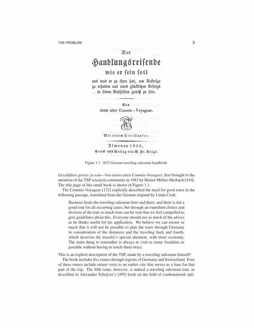
The numerous salesmen on the road were indeed interested in the planning of eco­nomical routes through their customer areas. An important reference in this context is the 1832 German handbook Der Handlungsreisende—wie er sein soll und was er zu thun hat, um Auftr¨ ucklichen Erfolgs in seinen age zu erhalten und eines gl¨

3 THE PROBLEM

Figure 1.1 1832 German traveling salesman handbook.

Geschaften gewiss zu sein—Von einem alten Commis-Voyageur, first brought to the attention of the TSP research community in 1983 by Heiner Muller-Merbach [410]. The title page of this small book is shown in Figure 1.1.

The Commis-Voyageur [132] explicitly described the need for good tours in the following passage, translated from the German original by Linda Cook.

Business leads the traveling salesman here and there, and there is not a good tour for all occurring cases; but through an expedient choice and division of the tour so much time can be won that we feel compelled to give guidelines about this. Everyone should use as much of the advice as he thinks useful for his application. We believe we can ensure as much that it will not be possible to plan the tours through Germany in consideration of the distances and the traveling back and fourth, which deserves the traveler’s special attention, with more economy. The main thing to remember is always to visit as many localities as possible without having to touch them twice.

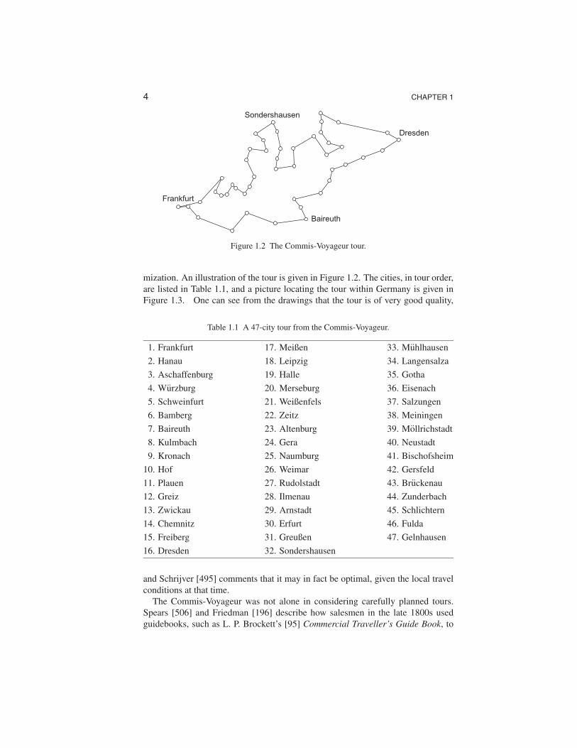
This is an explicit description of the TSP, made by a traveling salesman himself! The book includes five routes through regions of Germany and Switzerland. Four

of these routes include return visits to an earlier city that serves as a base for that part of the trip. The fifth route, however, is indeed a traveling salesman tour, as described in Alexander Schrijver’s [495] book on the field of combinatorial opti­

4 CHAPTER 1

Sondershausen

Baireuth

Frankfurt

Dresden

Figure 1.2 The Commis-Voyageur tour.

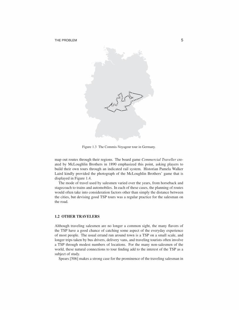
mization. An illustration of the tour is given in Figure 1.2. The cities, in tour order, are listed in Table 1.1, and a picture locating the tour within Germany is given in Figure 1.3. One can see from the drawings that the tour is of very good quality,

Table 1.1 A 47-city tour from the Commis-Voyageur.

1. Frankfurt 17. Meißen 33. Muhlhausen

2. Hanau 18. Leipzig 34. Langensalza

3. Aschaffenburg 19. Halle 35. Gotha

4. Wurzburg 20. Merseburg 36. Eisenach

5. Schweinfurt 21. Weißenfels 37. Salzungen

6. Bamberg 22. Zeitz 38. Meiningen

7. Baireuth 23. Altenburg 39. Mollrichstadt

8. Kulmbach 24. Gera 40. Neustadt

9. Kronach 25. Naumburg 41. Bischofsheim

10. Hof 26. Weimar 42. Gersfeld

11. Plauen 27. Rudolstadt 43. Bruckenau

12. Greiz 28. Ilmenau 44. Zunderbach

13. Zwickau 29. Arnstadt 45. Schlichtern

14. Chemnitz 30. Erfurt 46. Fulda

15. Freiberg 31. Greußen 47. Gelnhausen

16. Dresden 32. Sondershausen

and Schrijver [495] comments that it may in fact be optimal, given the local travel conditions at that time.

The Commis-Voyageur was not alone in considering carefully planned tours. Spears [506] and Friedman [196] describe how salesmen in the late 1800s used guidebooks, such as L. P. Brockett’s [95] Commercial Traveller’s Guide Book, to

5 THE PROBLEM

Figure 1.3 The Commis-Voyageur tour in Germany.

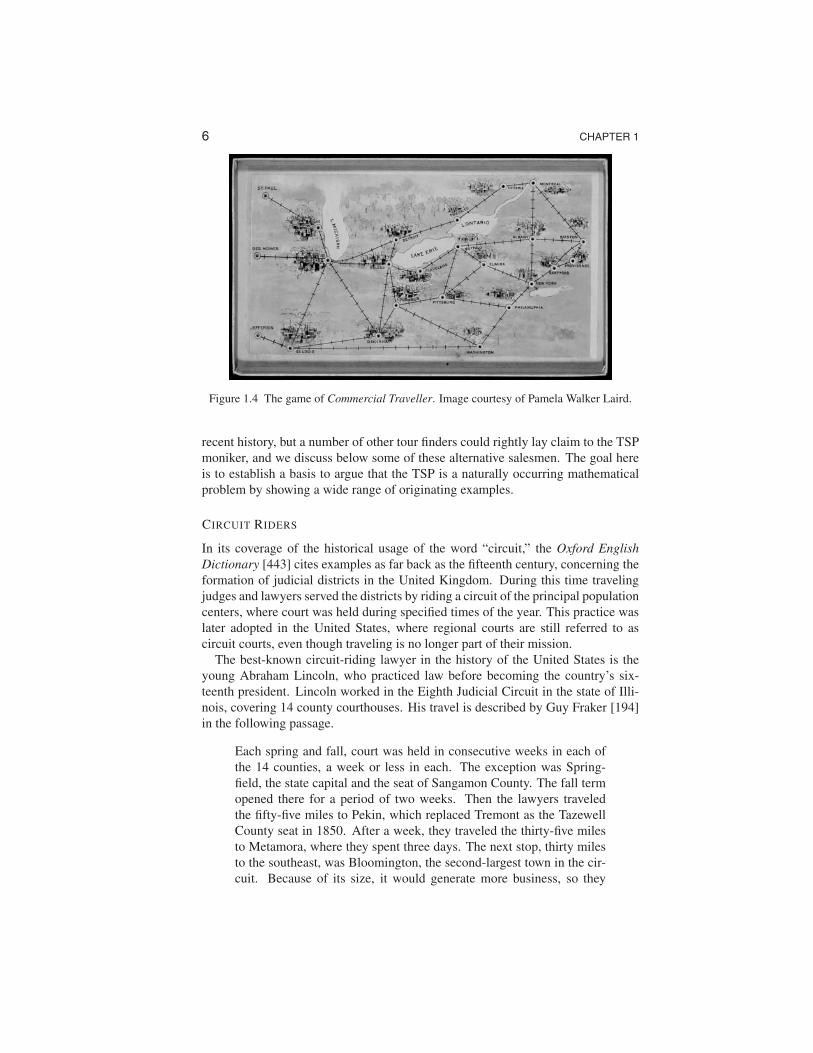
map out routes through their regions. The board game Commercial Traveller cre­ated by McLoughlin Brothers in 1890 emphasized this point, asking players to build their own tours through an indicated rail system. Historian Pamela Walker Laird kindly provided the photograph of the McLoughlin Brothers’ game that is displayed in Figure 1.4.

The mode of travel used by salesmen varied over the years, from horseback and stagecoach to trains and automobiles. In each of these cases, the planning of routes would often take into consideration factors other than simply the distance between the cities, but devising good TSP tours was a regular practice for the salesman on the road.

1.2 OTHER TRAVELERS

Although traveling salesmen are no longer a common sight, the many flavors of the TSP have a good chance of catching some aspect of the everyday experience of most people. The usual errand run around town is a TSP on a small scale, and longer trips taken by bus drivers, delivery vans, and traveling tourists often involve a TSP through modest numbers of locations. For the many non-salesmen of the world, these natural connections to tour finding add to the interest of the TSP as a subject of study.

Spears [506] makes a strong case for the prominence of the traveling salesman in

6 CHAPTER 1

Figure 1.4 The game of Commercial Traveller. Image courtesy of Pamela Walker Laird.

recent history, but a number of other tour finders could rightly lay claim to the TSP moniker, and we discuss below some of these alternative salesmen. The goal here is to establish a basis to argue that the TSP is a naturally occurring mathematical problem by showing a wide range of originating examples.

CIRCUIT RIDERS

In its coverage of the historical usage of the word “circuit,” the Oxford English Dictionary [443] cites examples as far back as the fifteenth century, concerning the formation of judicial districts in the United Kingdom. During this time traveling judges and lawyers served the districts by riding a circuit of the principal population centers, where court was held during specified times of the year. This practice was later adopted in the United States, where regional courts are still referred to as circuit courts, even though traveling is no longer part of their mission.

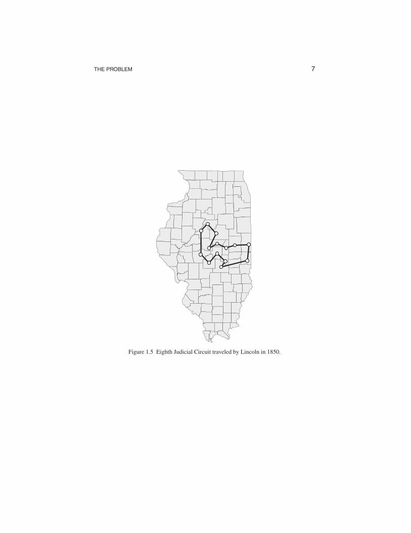
The best-known circuit-riding lawyer in the history of the United States is the young Abraham Lincoln, who practiced law before becoming the country’s six­teenth president. Lincoln worked in the Eighth Judicial Circuit in the state of Illi­nois, covering 14 county courthouses. His travel is described by Guy Fraker [194] in the following passage.

Each spring and fall, court was held in consecutive weeks in each of the 14 counties, a week or less in each. The exception was Spring­field, the state capital and the seat of Sangamon County. The fall term opened there for a period of two weeks. Then the lawyers traveled the fifty-five miles to Pekin, which replaced Tremont as the Tazewell County seat in 1850. After a week, they traveled the thirty-five miles to Metamora, where they spent three days. The next stop, thirty miles to the southeast, was Bloomington, the second-largest town in the cir­cuit. Because of its size, it would generate more business, so they

7 THE PROBLEM

Figure 1.5 Eighth Judicial Circuit traveled by Lincoln in 1850.

8 CHAPTER 1

would probably stay there several days longer. From there they would travel to Mt. Pulaski, seat of Logan County, a distance of thirty-five miles; it had replaced Postville as county seat in 1848 and would soon lose out to the new city of Lincoln, to be named for one of the men in this entourage. The travelers would then continue to another county and then another and another until they had completed the entire cir­cuit, taking a total of eleven weeks and traveling a distance of more than four hundred miles.

Fraker writes that Lincoln was one of the few court officials who regularly rode the entire circuit. A drawing of the route used by Lincoln and company in 1850 is given in Figure 1.5. Although the tour is not a shortest possible one (at least as the crow flies), it is clear that it was constructed with an eye toward minimizing the travel of the court personnel. The quality of Lincoln’s tour was pointed out several years ago in a TSP article by Jon Bentley [57].

Lincoln has drawn much attention to circuit-riding judges and lawyers, but as a group they are rivaled in fame by the circuit-riding Christian preachers of the eigh­teenth and nineteenth centuries. John Hampson [248] wrote the following passage in his 1791 biography of John Wesley, the founder of the Methodist church.

Every part of Britain and America is divided into regular portions, called circuits; and each circuit, containing twenty or thirty places, is supplied by a certain number of travelling preachers, from two to three or four, who go around it in a month or six weeks.

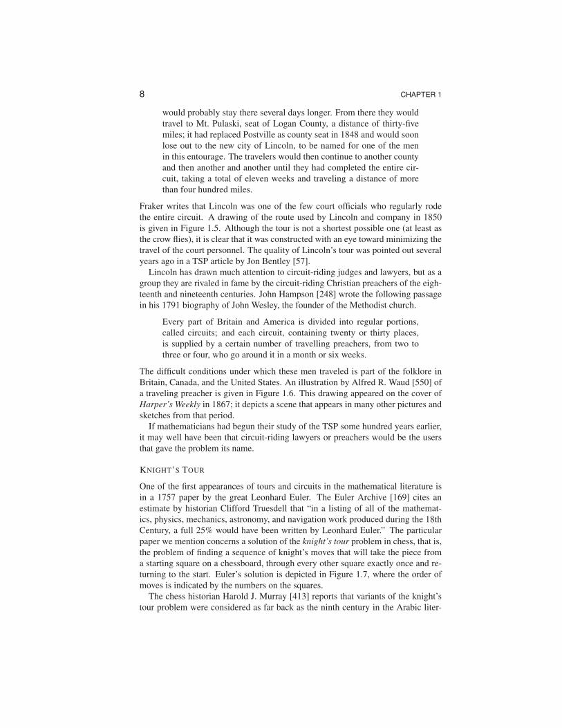
The difficult conditions under which these men traveled is part of the folklore in Britain, Canada, and the United States. An illustration by Alfred R. Waud [550] of a traveling preacher is given in Figure 1.6. This drawing appeared on the cover of Harper’s Weekly in 1867; it depicts a scene that appears in many other pictures and sketches from that period.

If mathematicians had begun their study of the TSP some hundred years earlier, it may well have been that circuit-riding lawyers or preachers would be the users that gave the problem its name.

KNIGHT’S TOUR

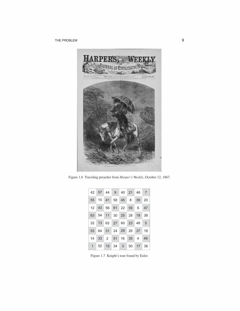
One of the first appearances of tours and circuits in the mathematical literature is in a 1757 paper by the great Leonhard Euler. The Euler Archive [169] cites an estimate by historian Clifford Truesdell that “in a listing of all of the mathemat­ics, physics, mechanics, astronomy, and navigation work produced during the 18th Century, a full 25% would have been written by Leonhard Euler.” The particular paper we mention concerns a solution of the knight’s tour problem in chess, that is, the problem of finding a sequence of knight’s moves that will take the piece from a starting square on a chessboard, through every other square exactly once and re­turning to the start. Euler’s solution is depicted in Figure 1.7, where the order of moves is indicated by the numbers on the squares.

The chess historian Harold J. Murray [413] reports that variants of the knight’s tour problem were considered as far back as the ninth century in the Arabic liter­

9 THE PROBLEM

Figure 1.6 Traveling preacher from Harper’s Weekly, October 12, 1867.

4 4914

13

57

43

54

52

41

162

20394555

36

28

219

59

23

50

8

35

61

30

27

51

34

58

33

10

53

5612

746404442

262464 18372931

22

173151

548606232

3819251163

476

Figure 1.7 Knight’s tour found by Euler.

10 CHAPTER 1

Gibraltar

Marseilles

Rome

Leghorn

Palermo Athens

Constantinople

Odessa Smyrna

Beirut

Alexandria

Palma

Malta Jerusalem

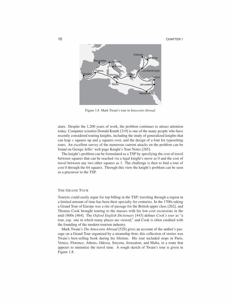
Figure 1.8 Mark Twain’s tour in Innocents Abroad.

ature. Despite the 1,200 years of work, the problem continues to attract attention today. Computer scientist Donald Knuth [319] is one of the many people who have recently considered touring knights, including the study of generalized knights that can leap x squares up and y squares over, and the design of a font for typesetting tours. An excellent survey of the numerous current attacks on the problem can be found on George Jellis’ web page Knight’s Tour Notes [285].

The knight’s problem can be formulated as a TSP by specifying the cost of travel between squares that can be reached via a legal knight’s move as 0 and the cost of travel between any two other squares as 1. The challenge is then to find a tour of cost 0 through the 64 squares. Through this view the knight’s problem can be seen as a precursor to the TSP.

THE GRAND TOUR

Tourists could easily argue for top billing in the TSP; traveling through a region in a limited amount of time has been their specialty for centuries. In the 1700s taking a Grand Tour of Europe was a rite of passage for the British upper class [262], and Thomas Cook brought touring to the masses with his low-cost excursions in the mid-1800s [464]. The Oxford English Dictionary [443] defines Cook’s tour as “a tour, esp. one in which many places are viewed,” and Cook is often credited with the founding of the modern tourism industry.

Mark Twain’s The Innocents Abroad [528] gives an account of the author’s pas­sage on a Grand Tour organized by a steamship firm; this collection of stories was Twain’s best-selling book during his lifetime. His tour included stops in Paris, Venice, Florence, Athens, Odessa, Smyrna, Jerusalem, and Malta, in a route that appears to minimize the travel time. A rough sketch of Twain’s tour is given in Figure 1.8.

11 THE PROBLEM

MESSENGERS

In the mathematics literature, it appears that the first mention of the TSP was made by Karl Menger, who described a variant of the problem in notes from a mathemat­ics colloquium held in Vienna on February 5, 1930 [389]. A rough translation of Menger’s problem from the German original is the following.

We use the term Botenproblem (because this question is faced in prac­tice by every postman, and by the way also by many travelers) for the task, given a finite number of points with known pairwise distances, to find the shortest path connecting the points.

So the problem is to find only a path through the points, without a return trip to the starting point. This version is easily converted to a TSP by adding an additional point having travel distance 0 to each of the original points.

Bote is the German word for messenger, so with Menger’s early proposal a case could be made for the use of the name messenger problem in place of TSP.

It is interesting that Menger mentions postmen in connection with the TSP, since in current mathematics terminology “postman problems” refers to another class of routing tasks, where the target is to traverse each of a specified set of roads rather than the cities joined by the roads. The motivation in this setting is that mail must be brought to houses that lie along the roads, so a full route should bring a postman along each road in his or her region. Early work on this topic was carried out by the Chinese mathematician Mei Gu Guan [240], who considered the version where the roads to be traversed are connected in the sense that it is possible to complete the travel without ever leaving the specified collection of roads. This special case was later dubbed the Chinese postman problem by Jack Edmonds in reference to Guan’s work. Remarkably, Edmonds [165] showed that the Chinese postman problem can always be solved efficiently (in a technical sense we discuss later in the chapter), whereas no such method appears on the horizon for the TSP itself.

In many settings, of course, a messenger or postman need not visit every house in a region, and in these cases the problem comes back to the TSP. In a recent publication, for example, Graham-Rowe [226] cites the use of TSP software to reduce the travel time of postmen in Denmark.

FARMLAND SURVEYS

Two of the earliest papers containing mathematical results concerning the TSP are by Eli S. Marks [375] and M. N. Ghosh [204], appearing in the late 1940s. The title of each of their papers includes the word “travel,” but their research was inspired by work concerning a traveling farmer rather than a traveling salesman. The statis­tician P. C. Mahalanobis described the original application in a 1940 research paper [368]. The work of Mahalanobis focused on the collection of data to make accurate forecasts of the jute crop in Bengal. A major source of revenue in India during the 1930s was derived from the export of raw and manufactured jute, accounting for roughly 1/4 of total exports during 1936–37. Furthermore, nearly 85% of India’s jute was grown in the Bengal region.

12 CHAPTER 1

A complete survey of the land in Bengal used in jute production was impractical, owing to the fact that it was grown on roughly 6 million small farms, scattered among some 80 million lots of all kinds. Mahalanobis proposed instead to make a random sample survey by dividing the country into zones comprising land of similar characteristics and within each zone select a random number of points to inspect for jute cultivation. One of the major components in the cost of making the survey was described by Mahalanobis as follows.

Journey, which includes the time spent in going from camp to camp (camp being defined as a place where the night is spent); from camp to a sample unit; and from sample unit to camp. This therefore cov­ers all journeys undertaken for the purpose of carrying out the field enumeration.

This is the TSP aspect of the application, to find efficient routes for the workers and equipment between the selected sites in the field.

It is interesting that, perhaps owing to his research interests as a statistician, Mahalanobis did not discuss the problem of finding tours for specific data but rather the problem of making statistical estimates of the expected length of an optimal tour for a random selection of locations. These estimates were included in projected costs of carrying out the survey, and thus were an important consideration in the decision to implement Mahalanobis’ plan in a small test in 1937 and in a large survey in 1938.

A similar “traveling farmer” problem was considered in the United States by Raymond J. Jessen, who wrote a report in 1942 on sampling farming regions in Iowa. Jessen [286] cites Mahalanobis’ results, but notes an important difference.

This relationship is based upon the assumption that points are con­nected by direct routes. In Iowa the road system is a quite regular net­work of mile square mesh. There are very few diagonal roads, there­fore, routes between points resemble those taken on a checkerboard.

The paper includes an empirical study of particular point sets under this checker­board distance function. We will see this type of travel cost again in Section 2.3 when we discuss applications of the TSP in the design of computer chips.

SCHOOL BUS ROUTING

We mentioned earlier a quote from Merrill Flood’s 1984 interview with Albert Tucker, citing a school bus routing problem as a source of his early interest in the TSP. Flood also made the following statement in a 1956 paper [182].

I am indebted to A. W. Tucker for calling these connections to my at­tention, in 1937, when I was struggling with the problem in connection with a school-bus routing study in New Jersey.

Note that Flood mentions New Jersey here and West Virginia in the earlier quote; it may well have been that he was involved in applications in several districts. Given the great importance of Flood’s contributions to the development of the TSP in the

13 THE PROBLEM

1940s and 1950s, the “school bus problem” would certainly have been a suitable alternative to the traveling salesman.

A van routing application did inspire one early research group to at least tem­porarily adopt the term “laundry van problem” in place of TSP, as described in a 1955 paper by G. Morton and A. H. Land [403].

In the United States this problem is known as the Travelling-salesman problem; the salesman wishes to visit one city in each of the 48 States and Washington, D. C., in such a sequence as to minimize total road distance travelled. Thinking of the problem independently and on a smaller geographical scale, we used to call it the laundry van problem, where the conditions were a daily service by a one-van laundry. Since the American term was used by Robinson (1949) we propose to adopt it here.

The Morton-Land name is clearly less “peppy” than the traveling salesman, but van routing is indeed an important application of the TSP.

WATCHMEN

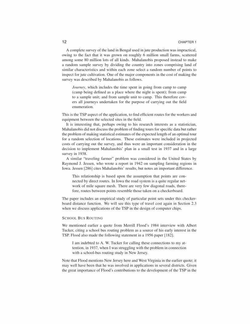
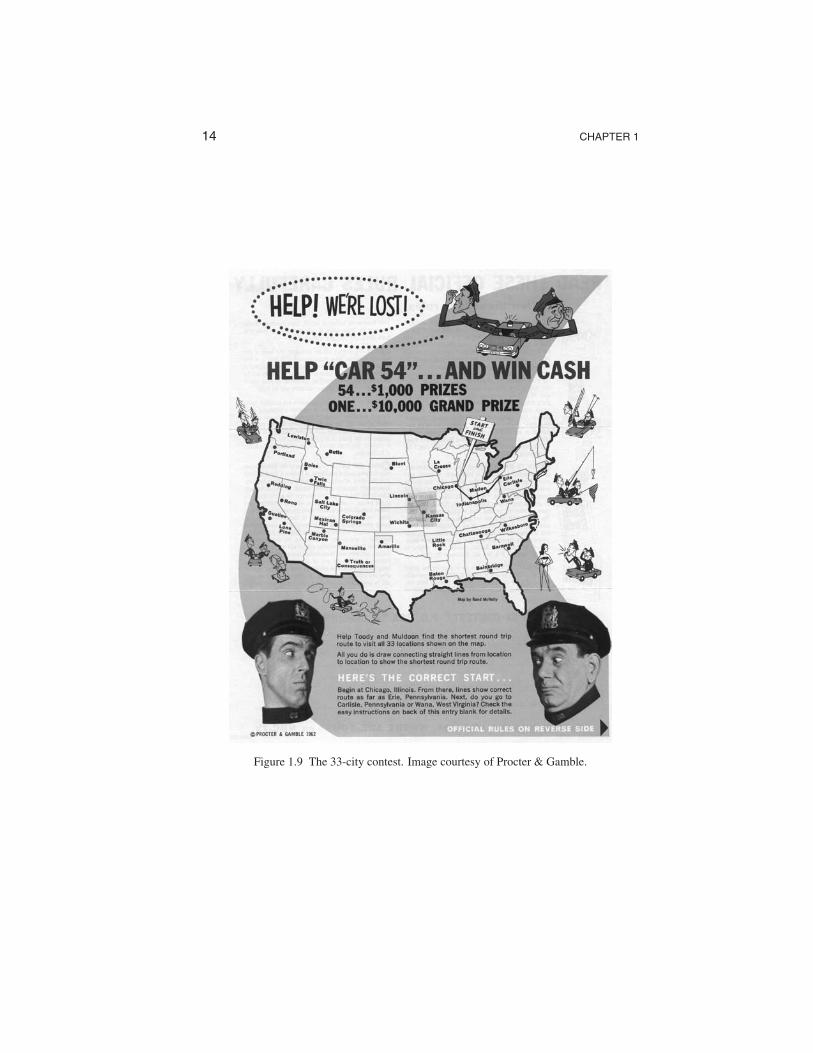
In the early 1960s, plotting a tour through the United States was in the public eye owing to an advertising campaign featuring a 33-city TSP. The original ad from Procter & Gamble is reproduced in Figure 1.9. The $10,000 prize for the shortest tour was huge at the time, enough to purchase a new house in many parts of the country. The proposed drivers of the tour were Toody and Muldoon, the police heroes of the Car 54, Where Are You? television series. Although the duty of these two officers did not actually go beyond the boundaries of New York’s Bronx borough, police and night watchmen must often walk or drive tours in their daily work.

The large prize money in the Procter & Gamble contest caught the attention of applied mathematicians; several papers on finding TSP tours cite this particular ex­ample. In fact, one of the winners of the contest was the TSP researcher Gerald Thompson of Carnegie Mellon University. Thompson coauthored a paper [304] with R. L. Karg in 1964 that reports the optimal tour displayed in Figure 1.10. It should be noted that Thompson did not know for sure that he had the shortest tour; there is a difference between finding a good tour and producing a convincing argu­ment that there is no tour of lesser cost. We discuss this point further in Chapters 3 and 4.

In a recent conversation Professor Thompson pointed out that a number of con­testants, including himself, had submitted the identical tour. The tiebreaker for the contest asked for a short essay on one of Procter & Gamble’s products, and we are happy to report that Thompson came through as a prize winner.

BOOK TOURS

Authors have a long history of being sent on far-reaching tours in promotion of their most recent works. Manil Suri, the author of the novel The Death of Vishnu [515], made the following remark in an interview in SIAM News in 2001 [516].

14 CHAPTER 1

Figure 1.9 The 33-city contest. Image courtesy of Procter & Gamble.

15 THE PROBLEM

Figure 1.10 Optimal 33-city tour.

The initial U.S. book tour, which starts January 24, 2001, will cover 13 cities in three weeks. When my publisher gave me the list of cities, I realized something amazing. I was actually going to live the Traveling Salesman Problem! I tried conveying my excitement to the publicity department, tried explaining to them the mathematical significance of all this, and how we could perhaps come up with an optimal solution, etc., etc. They were quite uneasy about my enthusiasm and assured me that they had lots of experience in planning itineraries, and would get back to me if they required mathematical assistance. So far, they haven’t.

Despite the reluctance of Suri’s publishers, book touring is another natural setting for the TSP and one that we see in action quite often.

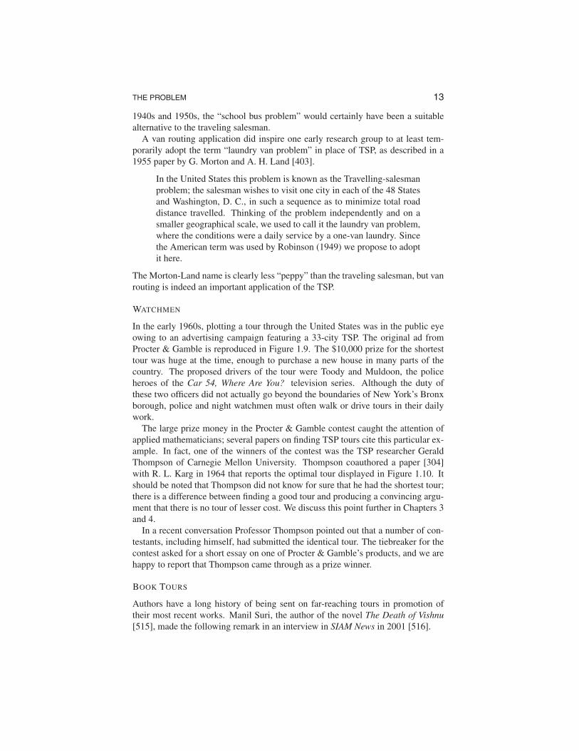
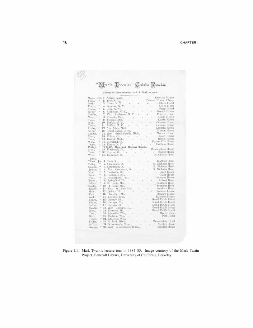
To get a feeling for the scope of tours made by authors, even as far back as the 1800s, consider the itinerary for a lecture tour made by Mark Twain in the winter of 1884–85, shown in Figure 1.11. The list in the figure describes only a portion of the travels of Twain and fellow writer George Washington Cable, who visited over 60 cities in their four-month tour of the United States and Canada [35].

1.3 GEOMETRY

When investigating a problem for solution ideas, most mathematicians will get out a pencil and draw a few figures to get things rolling. Geometric instances of the TSP, where cities are locations and the travel costs are distances between pairs, are tailor-made for such probing. In a single glance at a drawing of a tour we get a good measure of its quality.

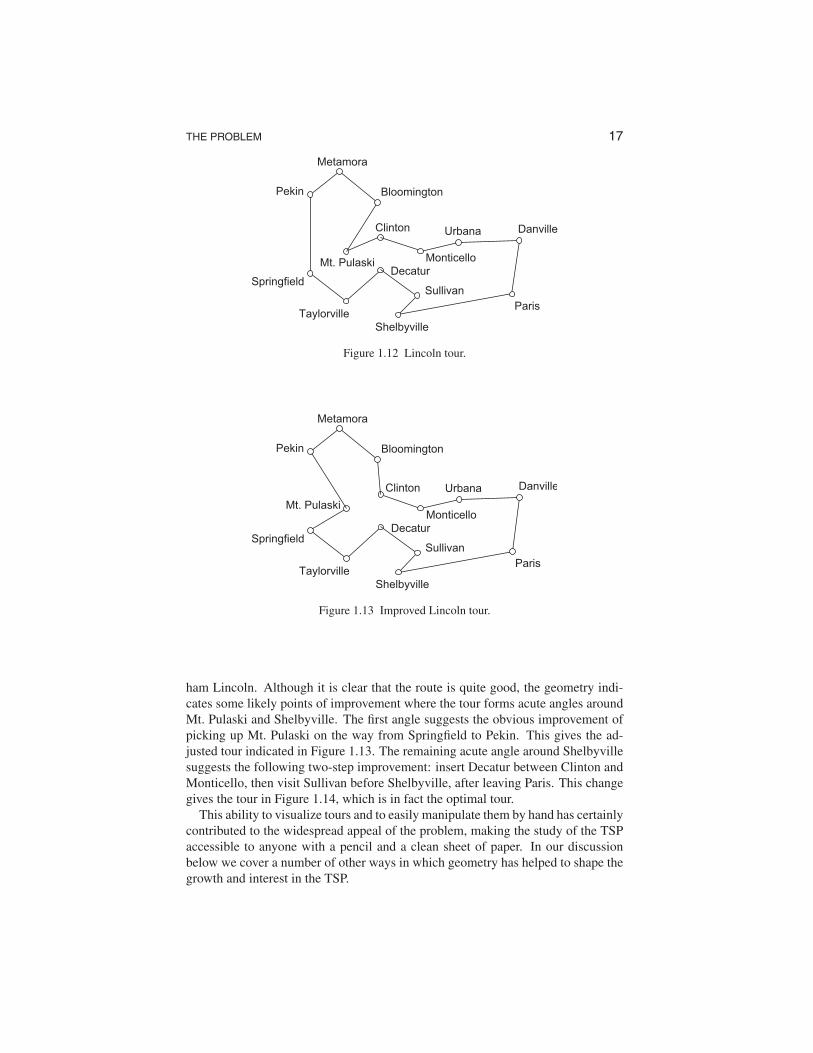
For example, in Figure 1.12 we give a closer view of the tour traveled by Abra­

16 CHAPTER 1

Figure 1.11 Mark Twain’s lecture tour in 1884–85. Image courtesy of the Mark Twain Project, Bancroft Library, University of California, Berkeley.

17 THE PROBLEM

Metamora

Pekin

Danville

Springfield

Paris

Bloomington

Taylorville

Shelbyville

Sullivan

Decatur Mt. Pulaski

Clinton

Monticello

Urbana

Figure 1.12 Lincoln tour.

Metamora

Pekin

Danville

Springfield

Paris

Bloomington

Taylorville

Shelbyville

Sullivan

Decatur

Monticello

Urbana

Mt. Pulaski

Clinton

Figure 1.13 Improved Lincoln tour.

ham Lincoln. Although it is clear that the route is quite good, the geometry indi­cates some likely points of improvement where the tour forms acute angles around Mt. Pulaski and Shelbyville. The first angle suggests the obvious improvement of picking up Mt. Pulaski on the way from Springfield to Pekin. This gives the ad­justed tour indicated in Figure 1.13. The remaining acute angle around Shelbyville suggests the following two-step improvement: insert Decatur between Clinton and Monticello, then visit Sullivan before Shelbyville, after leaving Paris. This change gives the tour in Figure 1.14, which is in fact the optimal tour.

This ability to visualize tours and to easily manipulate them by hand has certainly contributed to the widespread appeal of the problem, making the study of the TSP accessible to anyone with a pencil and a clean sheet of paper. In our discussion below we cover a number of other ways in which geometry has helped to shape the growth and interest in the TSP.

18 CHAPTER 1

Metamora

Pekin

Danville

Springfield

Paris

Clinton

Bloomington

Mt. Pulaski

Taylorville

Shelbyville

Decatur

Monticello

Sullivan

Urbana

Figure 1.14 Optimal Lincoln tour.

R

W S

DG F

K

TV

Q

NX

LJ

MH

CB

PZ

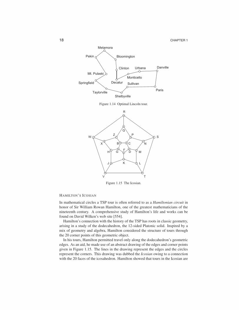
Figure 1.15 The Icosian.

HAMILTON’S ICOSIAN

In mathematical circles a TSP tour is often referred to as a Hamiltonian circuit in honor of Sir William Rowan Hamilton, one of the greatest mathematicians of the nineteenth century. A comprehensive study of Hamilton’s life and works can be found on David Wilken’s web site [554].

Hamilton’s connection with the history of the TSP has roots in classic geometry, arising in a study of the dodecahedron, the 12-sided Platonic solid. Inspired by a mix of geometry and algebra, Hamilton considered the structure of tours through the 20 corner points of this geometric object.

In his tours, Hamilton permitted travel only along the dodecahedron’s geometric edges. As an aid, he made use of an abstract drawing of the edges and corner points given in Figure 1.15. The lines in the drawing represent the edges and the circles represent the corners. This drawing was dubbed the Icosian owing to a connection with the 20 faces of the icosahedron. Hamilton showed that tours in the Icosian are

19 THE PROBLEM

both plentiful and flexible in that no matter what subpath of five points is chosen to start the path, it is always possible to complete the tour through the remaining 15 points and end up adjacent to the originating point. Fascinated with the elegance of this structure, Hamilton described his work as a game in a letter from 1856 [246].

I have found that some young persons have been much amused by trying a new mathematical game which the Icosian furnishes, one per­son sticking five pins in any five consecutive points, such as abcde, or abcde′, and the other player then aiming to insert, which by the theory in this letter can always be done, fifteen other pins, in cyclincal suc­cession, so as to cover all the other points, and to end in immediate proximity to the pin wherewith his antagonist had begun.

In the following year, Hamilton presented his work on the Icosian at a scientific meeting held in Dublin. The report from the meeting [94] included the following passage.

The author stated that this calculus was entirely distinct from that of quaternions, and in it none of the roots concerned were imaginary. He then explained the leading features of the new calculus, and exem­plified its use by an amusing game, which he called the Icosian, and which he had been led to invent by it, — a lithograph of which he dis­tributed through the Section, and examples of what the game proposed to be accomplished were lithographed in the margin, the solutions be­ing shown to be exemplifications of the calculus. The figure was the projection on a plane of the regular pentagonal dodecahedron, and at each of the angles were holes for receiving the ivory pins with which the game was played.

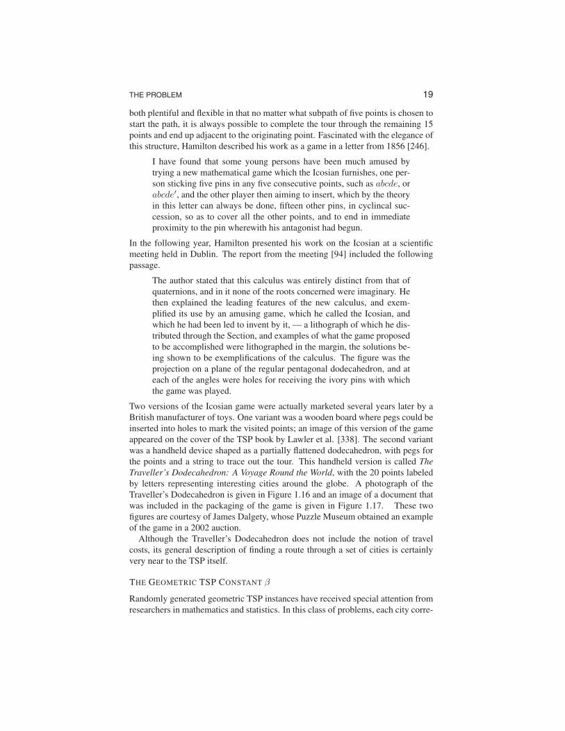
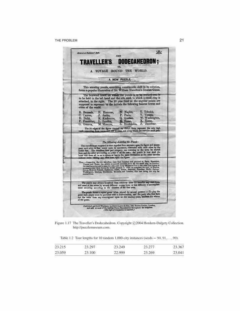
Two versions of the Icosian game were actually marketed several years later by a British manufacturer of toys. One variant was a wooden board where pegs could be inserted into holes to mark the visited points; an image of this version of the game appeared on the cover of the TSP book by Lawler et al. [338]. The second variant was a handheld device shaped as a partially flattened dodecahedron, with pegs for the points and a string to trace out the tour. This handheld version is called The Traveller’s Dodecahedron: A Voyage Round the World, with the 20 points labeled by letters representing interesting cities around the globe. A photograph of the Traveller’s Dodecahedron is given in Figure 1.16 and an image of a document that was included in the packaging of the game is given in Figure 1.17. These two figures are courtesy of James Dalgety, whose Puzzle Museum obtained an example of the game in a 2002 auction.

Although the Traveller’s Dodecahedron does not include the notion of travel costs, its general description of finding a route through a set of cities is certainly very near to the TSP itself.

THE GEOMETRIC TSP CONSTANT β

Randomly generated geometric TSP instances have received special attention from researchers in mathematics and statistics. In this class of problems, each city corre­

20 CHAPTER 1

cDalgety Collection. http://puzzlemuseum.com.

Figure 1.16 The Traveller’s Dodecahedron handheld game. Copyright ©2006 Hordern­

sponds to a point chosen independently and uniformly from the unit square, that is, each point (x, y) with both x and y between 0 and 1 is equally likely to be selected as a city. The cost of travel between cities is measured by the usual Euclidean dis­tance. These instances were targeted for study by Mahalanobis [368] in connection with his work on farmland surveys.

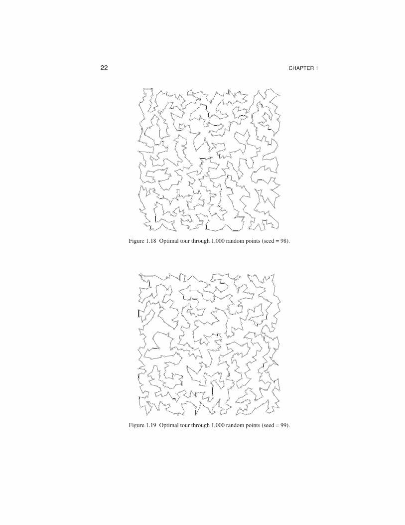
Although it may seem surprising, instances from this class of random problems are actually quite similar to one another. For example, consider the pair of 1,000­city tours shown in Figures 1.18 and 1.19. The displayed tours are optimal for the problems obtained by scaling the travel costs by 1,000,000 and rounding to the nearest integer, to avoid the difficulty of working with square roots when comparing distances. Now, at first glance, it is not so easy to see the difference between the two pictures.

The tours in the figures have lengths approximately 23.269 and 23.041 respec­tively. The proximity of these values is not a coincidence. In Table 1.2 we list the lengths for 10 random 1,000-city tours; a quick inspection shows that they are all relatively close in value. The problem that intrigued Mahalanobis [368] and many others is to determine what can be said in general about the distribution of tour lengths for random geometric problems on n cities.

Clearly, the length of tours we expect to obtain will increase as n gets larger. Mahalanobis [368] makes an argument that the lengths should grow roughly in proportion to

√n, and a formal proof of this was given by Marks [375] and Ghosh

[204]. This pair of researchers attacked the problem from two sides, Ghosh show­ing that the expected length of an optimal tour is no more than 1.27

√n and Marks

showing that the expected length is at least (√n − 1/

√n)/

√2.

21 THE PROBLEM

cFigure 1.17 The Traveller’s Dodecahedron. Copyright ©2004 Hordern-Dalgety Collection. http://puzzlemuseum.com.

Table 1.2 Tour lengths for 10 random 1,000-city instances (seeds = 90, 91,. . . , 99).

23.215 23.297 23.249 23.277 23.367

23.059 23.100 22.999 23.269 23.041

22 CHAPTER 1

Figure 1.18 Optimal tour through 1,000 random points (seed = 98).

Figure 1.19 Optimal tour through 1,000 random points (seed = 99).

23 THE PROBLEM

500

400

300

200

100

0 0.71 0.72 0.73 0.74 0.75

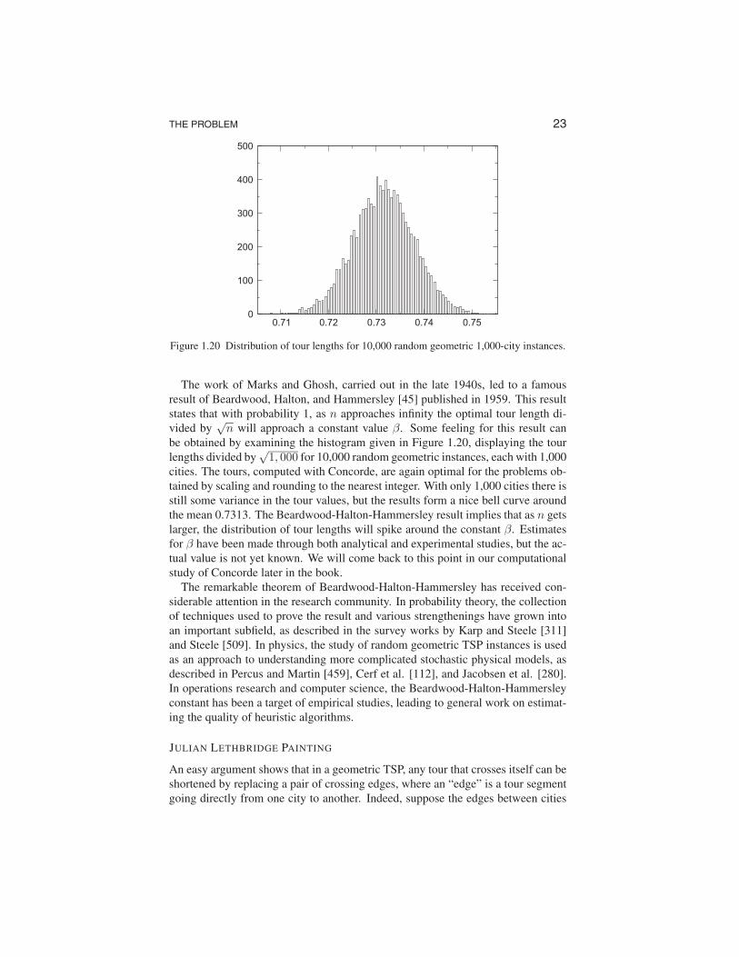
Figure 1.20 Distribution of tour lengths for 10,000 random geometric 1,000-city instances.

The work of Marks and Ghosh, carried out in the late 1940s, led to a famous result of Beardwood, Halton, and Hammersley [45] published in 1959. This result states that with probability 1, as n approaches infinity the optimal tour length di­vided by

√n will approach a constant value β. Some feeling for this result can

be obtained by examining the histogram given in Figure 1.20, displaying the tour lengths divided by

√1, 000 for 10,000 random geometric instances, each with 1,000

cities. The tours, computed with Concorde, are again optimal for the problems ob­tained by scaling and rounding to the nearest integer. With only 1,000 cities there is still some variance in the tour values, but the results form a nice bell curve around the mean 0.7313. The Beardwood-Halton-Hammersley result implies that as n gets larger, the distribution of tour lengths will spike around the constant β. Estimates for β have been made through both analytical and experimental studies, but the ac­tual value is not yet known. We will come back to this point in our computational study of Concorde later in the book.

The remarkable theorem of Beardwood-Halton-Hammersley has received con­siderable attention in the research community. In probability theory, the collection of techniques used to prove the result and various strengthenings have grown into an important subfield, as described in the survey works by Karp and Steele [311] and Steele [509]. In physics, the study of random geometric TSP instances is used as an approach to understanding more complicated stochastic physical models, as described in Percus and Martin [459], Cerf et al. [112], and Jacobsen et al. [280]. In operations research and computer science, the Beardwood-Halton-Hammersley constant has been a target of empirical studies, leading to general work on estimat­ing the quality of heuristic algorithms.

JULIAN LETHBRIDGE PAINTING

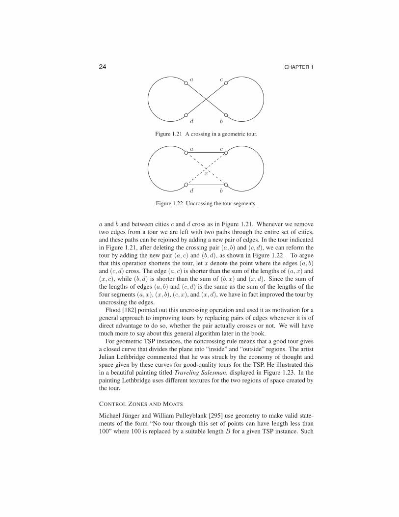
An easy argument shows that in a geometric TSP, any tour that crosses itself can be shortened by replacing a pair of crossing edges, where an “edge” is a tour segment going directly from one city to another. Indeed, suppose the edges between cities

24 CHAPTER 1

b

c

d

a

Figure 1.21 A crossing in a geometric tour.

b

c

d

a

x

Figure 1.22 Uncrossing the tour segments.

a and b and between cities c and d cross as in Figure 1.21. Whenever we remove two edges from a tour we are left with two paths through the entire set of cities, and these paths can be rejoined by adding a new pair of edges. In the tour indicated in Figure 1.21, after deleting the crossing pair (a, b) and (c, d), we can reform the tour by adding the new pair (a, c) and (b, d), as shown in Figure 1.22. To argue that this operation shortens the tour, let x denote the point where the edges (a, b) and (c, d) cross. The edge (a, c) is shorter than the sum of the lengths of (a, x) and (x, c), while (b, d) is shorter than the sum of (b, x) and (x, d). Since the sum of the lengths of edges (a, b) and (c, d) is the same as the sum of the lengths of the four segments (a, x), (x, b), (c, x), and (x, d), we have in fact improved the tour by uncrossing the edges.

Flood [182] pointed out this uncrossing operation and used it as motivation for a general approach to improving tours by replacing pairs of edges whenever it is of direct advantage to do so, whether the pair actually crosses or not. We will have much more to say about this general algorithm later in the book.

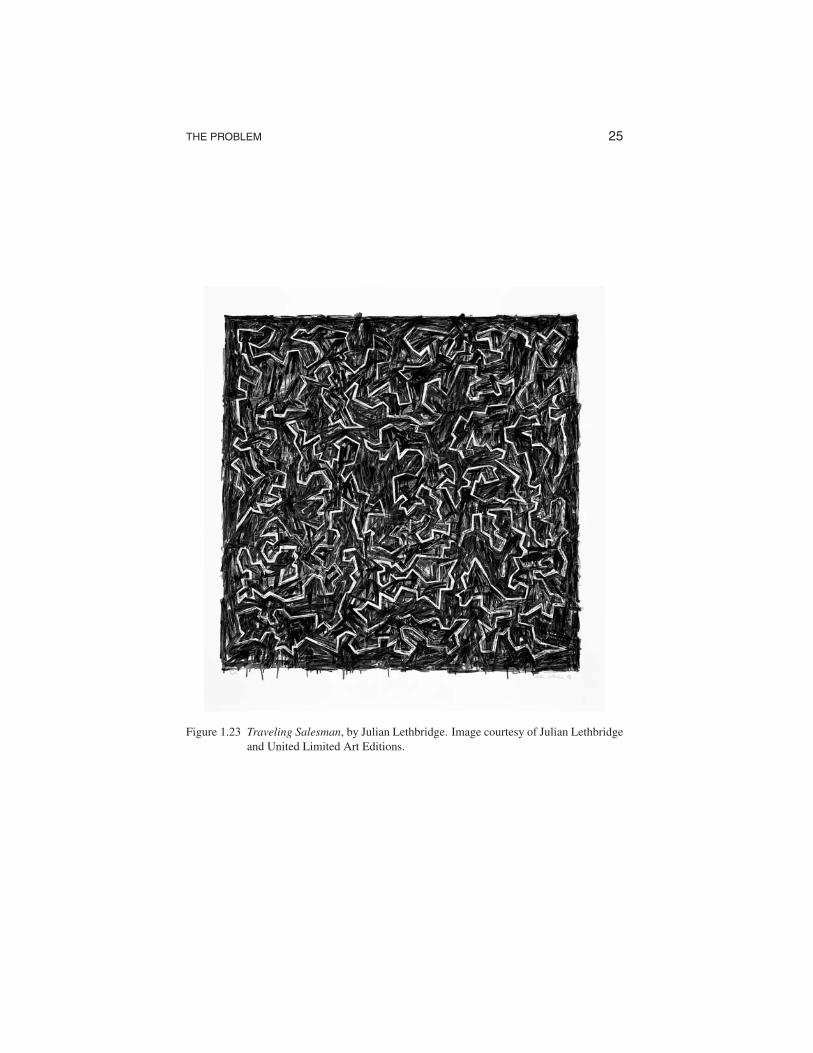
For geometric TSP instances, the noncrossing rule means that a good tour gives a closed curve that divides the plane into “inside” and “outside” regions. The artist Julian Lethbridge commented that he was struck by the economy of thought and space given by these curves for good-quality tours for the TSP. He illustrated this in a beautiful painting titled Traveling Salesman, displayed in Figure 1.23. In the painting Lethbridge uses different textures for the two regions of space created by the tour.

CONTROL ZONES AND MOATS

Michael Junger and William Pulleyblank [295] use geometry to make valid state­ments of the form “No tour through this set of points can have length less than 100” where 100 is replaced by a suitable length B for a given TSP instance. Such

25 THE PROBLEM

Figure 1.23 Traveling Salesman, by Julian Lethbridge. Image courtesy of Julian Lethbridge and United Limited Art Editions.

26 CHAPTER 1

a number B is called a lower bound for the TSP since it bounds from below the length of all tours.

The importance of lower bounds is that they can be used to certify that a tour we may have found is good, or even best, when compared to all of the other tours that we have not considered. A more direct approach would of course be to simply con­sider all possible tours, but this number grows so quickly that checking all of them for a modest-size instance, say 50 cities, is well beyond the capabilities of even the fastest of today’s supercomputers. Carefully constructed lower bounds provide a more subtle way to make conclusions about the lengths of all tours through a set of points.

There are a number of different strategies for finding good lower bounds for the TSP. In Concorde and in other modern solvers, the bounding technique of choice goes back to George Dantzig, Ray Fulkerson, and Selmer Johnson [151], who in 1954 had the first major success in the solution of the TSP. For geometric problems, Junger and Pulleyblank have shown that some of the basic ideas employed by this research team have a simple geometric interpretation, as we now describe.

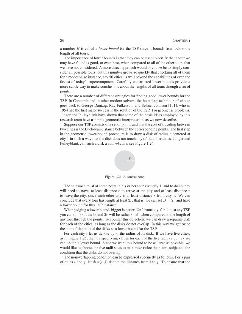
Suppose our TSP consists of a set of points and that the cost of traveling between two cities is the Euclidean distance between the corresponding points. The first step in the geometric lower-bound procedure is to draw a disk of radius r centered at city 1 in such a way that the disk does not touch any of the other cities. Junger and Pulleyblank call such a disk a control zone; see Figure 1.24.

r

Figure 1.24 A control zone.

The salesman must at some point in his or her tour visit city 1, and to do so they will need to travel at least distance r to arrive at the city and at least distance r to leave the city, since each other city is at least distance r from city 1. We can conclude that every tour has length at least 2r, that is, we can set B = 2r and have a lower bound for this TSP instance.

When judging a lower bound, bigger is better. Unfortunately, for almost any TSP you can think of, the bound 2r will be rather small when compared to the length of any tour through the points. To counter this objection, we can draw a separate disk for each of the cities, as long as the disks do not overlap. In this way we get twice the sum of the radii of the disks as a lower bound for the TSP.

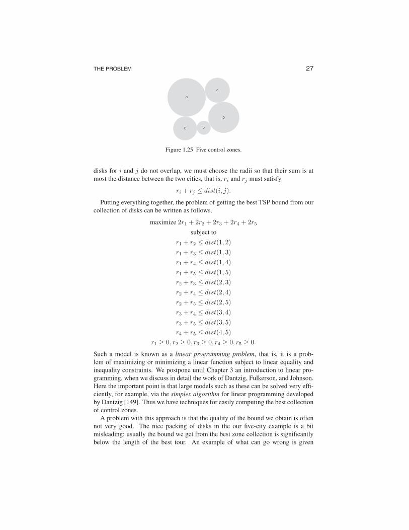
For each city i let us denote by ri the radius of its disk. If we have five cities, as in Figure 1.25, then by specifying values for each of the five radii r1, . . . , r5 we can obtain a lower bound. Since we want this bound to be as large as possible, we would like to choose the five radii so as to maximize twice their sum, subject to the condition that the disks do not overlap.

The nonoverlapping condition can be expressed succinctly as follows. For a pair of cities i and j, let dist(i, j) denote the distance from i to j. To ensure that the

27 THE PROBLEM

Figure 1.25 Five control zones.

disks for i and j do not overlap, we must choose the radii so that their sum is at most the distance between the two cities, that is, ri and rj must satisfy

ri + rj ≤ dist(i, j).

Putting everything together, the problem of getting the best TSP bound from our collection of disks can be written as follows.

maximize 2r1 + 2r2 + 2r3 + 2r4 + 2r5

subject to

r1 + r2 ≤ dist(1, 2)r1 + r3 ≤ dist(1, 3)r1 + r4 ≤ dist(1, 4)r1 + r5 ≤ dist(1, 5)r2 + r3 ≤ dist(2, 3)r2 + r4 ≤ dist(2, 4)r2 + r5 ≤ dist(2, 5)r3 + r4 ≤ dist(3, 4)r3 + r5 ≤ dist(3, 5)r4 + r5 ≤ dist(4, 5)

r1 ≥ 0, r2 ≥ 0, r3 ≥ 0, r4 ≥ 0, r5 ≥ 0.

Such a model is known as a linear programming problem, that is, it is a prob­lem of maximizing or minimizing a linear function subject to linear equality and inequality constraints. We postpone until Chapter 3 an introduction to linear pro­gramming, when we discuss in detail the work of Dantzig, Fulkerson, and Johnson. Here the important point is that large models such as these can be solved very effi­ciently, for example, via the simplex algorithm for linear programming developed by Dantzig [149]. Thus we have techniques for easily computing the best collection of control zones.

A problem with this approach is that the quality of the bound we obtain is often not very good. The nice packing of disks in the our five-city example is a bit misleading; usually the bound we get from the best zone collection is significantly below the length of the best tour. An example of what can go wrong is given

28 CHAPTER 1

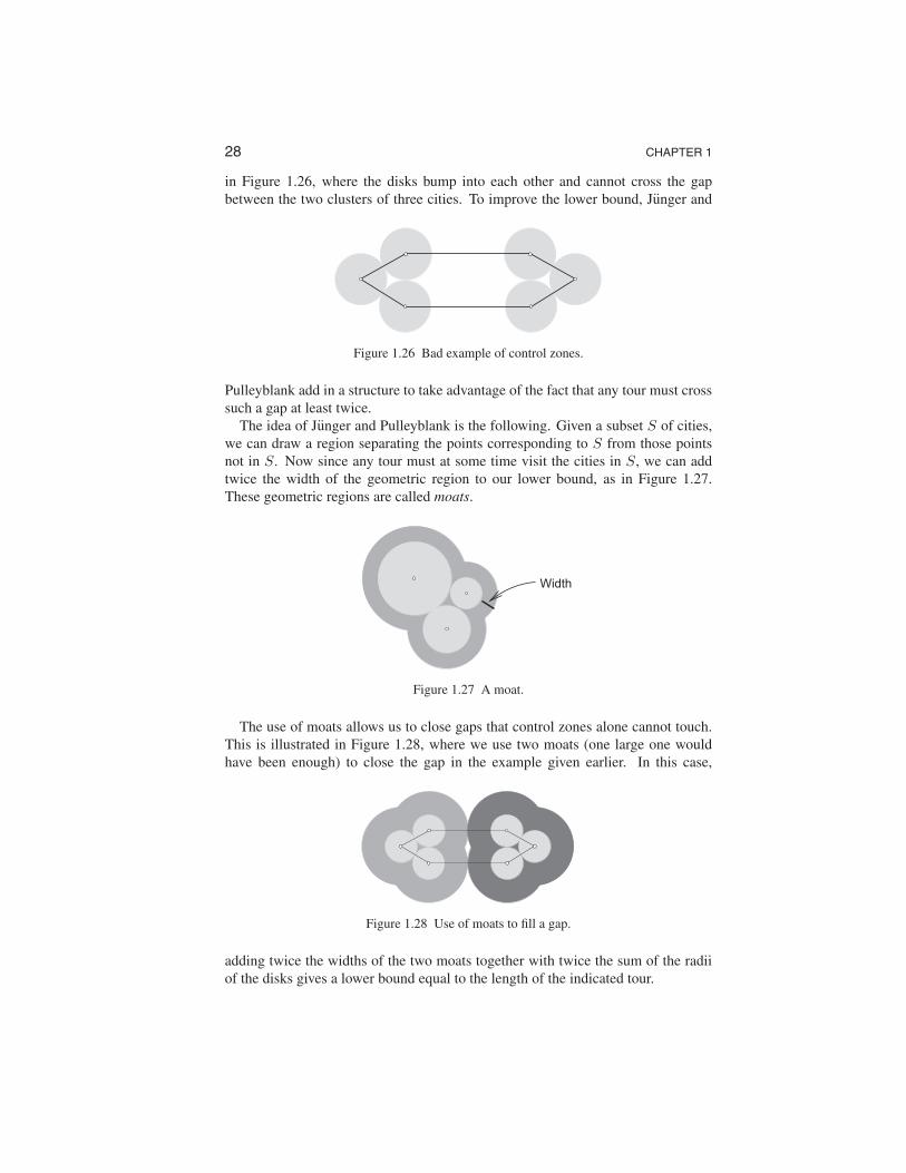
in Figure 1.26, where the disks bump into each other and cannot cross the gap between the two clusters of three cities. To improve the lower bound, Junger and

Figure 1.26 Bad example of control zones.

Pulleyblank add in a structure to take advantage of the fact that any tour must cross such a gap at least twice.

The idea of Junger and Pulleyblank is the following. Given a subset S of cities, we can draw a region separating the points corresponding to S from those points not in S. Now since any tour must at some time visit the cities in S, we can add twice the width of the geometric region to our lower bound, as in Figure 1.27. These geometric regions are called moats.

Width

Figure 1.27 A moat.

The use of moats allows us to close gaps that control zones alone cannot touch. This is illustrated in Figure 1.28, where we use two moats (one large one would have been enough) to close the gap in the example given earlier. In this case,

Figure 1.28 Use of moats to fill a gap.

adding twice the widths of the two moats together with twice the sum of the radii of the disks gives a lower bound equal to the length of the indicated tour.

29 THE PROBLEM

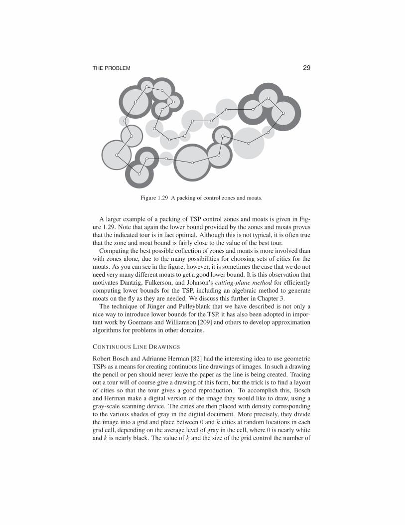
Figure 1.29 A packing of control zones and moats.

A larger example of a packing of TSP control zones and moats is given in Fig­ure 1.29. Note that again the lower bound provided by the zones and moats proves that the indicated tour is in fact optimal. Although this is not typical, it is often true that the zone and moat bound is fairly close to the value of the best tour.

Computing the best possible collection of zones and moats is more involved than with zones alone, due to the many possibilities for choosing sets of cities for the moats. As you can see in the figure, however, it is sometimes the case that we do not need very many different moats to get a good lower bound. It is this observation that motivates Dantzig, Fulkerson, and Johnson’s cutting-plane method for efficiently computing lower bounds for the TSP, including an algebraic method to generate moats on the fly as they are needed. We discuss this further in Chapter 3.

The technique of Junger and Pulleyblank that we have described is not only a nice way to introduce lower bounds for the TSP, it has also been adopted in impor­tant work by Goemans and Williamson [209] and others to develop approximation algorithms for problems in other domains.

CONTINUOUS LINE DRAWINGS

Robert Bosch and Adrianne Herman [82] had the interesting idea to use geometric TSPs as a means for creating continuous line drawings of images. In such a drawing the pencil or pen should never leave the paper as the line is being created. Tracing out a tour will of course give a drawing of this form, but the trick is to find a layout of cities so that the tour gives a good reproduction. To accomplish this, Bosch and Herman make a digital version of the image they would like to draw, using a gray-scale scanning device. The cities are then placed with density corresponding to the various shades of gray in the digital document. More precisely, they divide the image into a grid and place between 0 and k cities at random locations in each grid cell, depending on the average level of gray in the cell, where 0 is nearly white and k is nearly black. The value of k and the size of the grid control the number of

30 CHAPTER 1

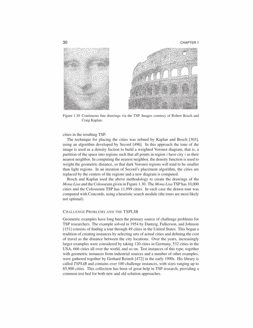
Figure 1.30 Continuous line drawings via the TSP. Images courtesy of Robert Bosch and Craig Kaplan.

cities in the resulting TSP. The technique for placing the cities was refined by Kaplan and Bosch [303],

using an algorithm developed by Secord [496]. In this approach the tone of the image is used as a density fuction to build a weighted Voronoi diagram, that is, a partition of the space into regions such that all points in region i have city i as their nearest neighbor. In computing the nearest neighbor, the density function is used to weight the geometric distance, so that dark Voronoi regions will tend to be smaller than light regions. In an iteration of Secord’s placement algorithm, the cities are replaced by the centers of the regions and a new diagram is computed.

Bosch and Kaplan used the above methodology to create the drawings of the Mona Lisa and the Colosseum given in Figure 1.30. The Mona Lisa TSP has 10,000 cities and the Colosseum TSP has 11,999 cities. In each case the drawn tour was computed with Concorde, using a heuristic search module (the tours are most likely not optimal).

CHALLENGE PROBLEMS AND THE TSPLIB

Geometric examples have long been the primary source of challenge problems for TSP researchers. The example solved in 1954 by Dantzig, Fulkerson, and Johnson [151] consists of finding a tour through 49 cities in the United States. This began a tradition of creating instances by selecting sets of actual cities and defining the cost of travel as the distance between the city locations. Over the years, increasingly larger examples were considered by taking 120 cities in Germany, 532 cities in the USA, 666 cities all over the world, and so on. Test instances of this type, together with geometric instances from industrial sources and a number of other examples, were gathered together by Gerhard Reinelt [472] in the early 1990s. His library is called TSPLIB and contains over 100 challenge instances, with sizes ranging up to 85,900 cities. This collection has been of great help in TSP research, providing a common test bed for both new and old solution approaches.

31 THE PROBLEM

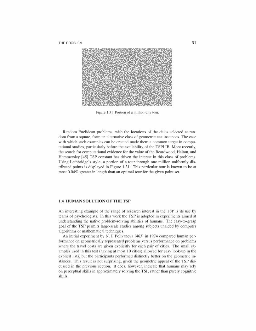
Figure 1.31 Portion of a million-city tour.

Random Euclidean problems, with the locations of the cities selected at ran­dom from a square, form an alternative class of geometric test instances. The ease with which such examples can be created made them a common target in compu­tational studies, particularly before the availability of the TSPLIB. More recently, the search for computational evidence for the value of the Beardwood, Halton, and Hammersley [45] TSP constant has driven the interest in this class of problems. Using Lethbridge’s style, a portion of a tour through one million uniformly dis­tributed points is displayed in Figure 1.31. This particular tour is known to be at most 0.04% greater in length than an optimal tour for the given point set.

1.4 HUMAN SOLUTION OF THE TSP

An interesting example of the range of research interest in the TSP is its use by teams of psychologists. In this work the TSP is adopted in experiments aimed at understanding the native problem-solving abilities of humans. The easy-to-grasp goal of the TSP permits large-scale studies among subjects unaided by computer algorithms or mathematical techniques.

An initial experiment by N. I. Polivanova [463] in 1974 compared human per­formance on geometrically represented problems versus performance on problems where the travel costs are given explicitly for each pair of cities. The small ex­amples used in this test (having at most 10 cities) allowed for easy look-up in the explicit lists, but the participants performed distinctly better on the geometric in­stances. This result is not surprising, given the geometric appeal of the TSP dis­cussed in the previous section. It does, however, indicate that humans may rely on perceptual skills in approximately solving the TSP, rather than purely cognitive skills.

32 CHAPTER 1

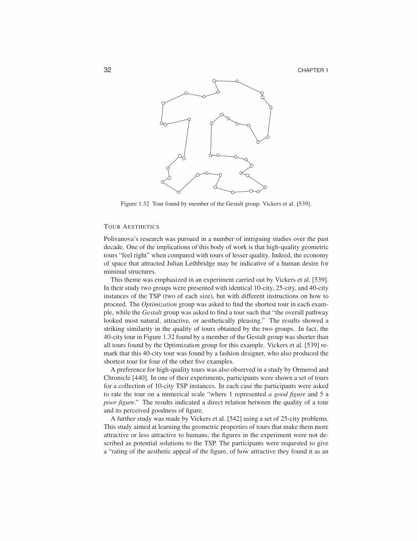
Figure 1.32 Tour found by member of the Gestalt group. Vickers et al. [539].

TOUR AESTHETICS

Polivanova’s research was pursued in a number of intriguing studies over the past decade. One of the implications of this body of work is that high-quality geometric tours “feel right” when compared with tours of lesser quality. Indeed, the economy of space that attracted Julian Lethbridge may be indicative of a human desire for minimal structures.

This theme was emphasized in an experiment carried out by Vickers et al. [539]. In their study two groups were presented with identical 10-city, 25-city, and 40-city instances of the TSP (two of each size), but with different instructions on how to proceed. The Optimization group was asked to find the shortest tour in each exam­ple, while the Gestalt group was asked to find a tour such that “the overall pathway looked most natural, attractive, or aesthetically pleasing.” The results showed a striking similarity in the quality of tours obtained by the two groups. In fact, the 40-city tour in Figure 1.32 found by a member of the Gestalt group was shorter than all tours found by the Optimization group for this example. Vickers et al. [539] re­mark that this 40-city tour was found by a fashion designer, who also produced the shortest tour for four of the other five examples.

A preference for high-quality tours was also observed in a study by Ormerod and Chronicle [440]. In one of their experiments, participants were shown a set of tours for a collection of 10-city TSP instances. In each case the participants were asked to rate the tour on a numerical scale “where 1 represented a good figure and 5 a poor figure.” The results indicated a direct relation between the quality of a tour and its perceived goodness of figure.

A further study was made by Vickers et al. [542] using a set of 25-city problems. This study aimed at learning the geometric properties of tours that make them more attractive or less attractive to humans; the figures in the experiment were not de­scribed as potential solutions to the TSP. The participants were requested to give a “rating of the aesthetic appeal of the figure, of how attractive they found it as an

33 THE PROBLEM

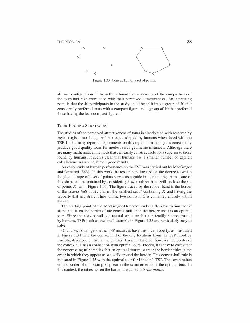
Figure 1.33 Convex hull of a set of points.

abstract configuration.” The authors found that a measure of the compactness of the tours had high correlation with their perceived attractiveness. An interesting point is that the 40 participants in the study could be split into a group of 30 that consistently preferred tours with a compact figure and a group of 10 that preferred those having the least compact figure.

TOUR-FINDING STRATEGIES

The studies of the perceived attractiveness of tours is closely tied with research by psychologists into the general strategies adopted by humans when faced with the TSP. In the many reported experiments on this topic, human subjects consistently produce good-quality tours for modest-sized geometric instances. Although there are many mathematical methods that can easily construct solutions superior to those found by humans, it seems clear that humans use a smaller number of explicit calculations in arriving at their good results.

An early study of human performance on the TSP was carried out by MacGregor and Ormerod [363]. In this work the researchers focused on the degree to which the global shape of a set of points serves as a guide in tour finding. A measure of this shape can be obtained by considering how a rubber band will enclose the set of points X , as in Figure 1.33. The figure traced by the rubber band is the border of the convex hull of X , that is, the smallest set S containing X and having the property that any straight line joining two points in S is contained entirely within the set.

The starting point of the MacGregor-Ormerod study is the observation that if all points lie on the border of the convex hull, then the border itself is an optimal tour. Since the convex hull is a natural structure that can readily be constructed by humans, TSPs such as the small example in Figure 1.33 are particularly easy to solve.

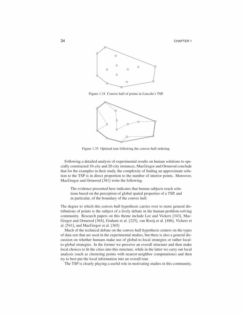
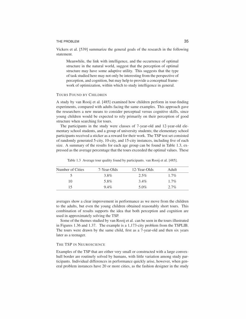
Of course, not all geometric TSP instances have this nice property, as illustrated in Figure 1.34 with the convex hull of the city locations from the TSP faced by Lincoln, described earlier in the chapter. Even in this case, however, the border of the convex hull has a connection with optimal tours. Indeed, it is easy to check that the noncrossing rule implies that an optimal tour must trace the border cities in the order in which they appear as we walk around the border. This convex-hull rule is indicated in Figure 1.35 with the optimal tour for Lincoln’s TSP. The seven points on the border of this example appear in the same order as in the optimal tour. In this context, the cities not on the border are called interior points.

34 CHAPTER 1

Figure 1.34 Convex hull of points in Lincoln’s TSP.

Figure 1.35 Optimal tour following the convex-hull ordering.

Following a detailed analysis of experimental results on human solutions to spe­cially constructed 10-city and 20-city instances, MacGregor and Ormerod conclude that for the examples in their study, the complexity of finding an approximate solu­tion to the TSP is in direct proportion to the number of interior points. Moreover, MacGregor and Ormerod [381] write the following.

The evidence presented here indicates that human subjects reach solu­tions based on the perception of global spatial properties of a TSP, and in particular, of the boundary of the convex hull.

The degree to which this convex-hull hypothesis carries over to more general dis­tributions of points is the subject of a lively debate in the human-problem-solving community. Research papers on this theme include Lee and Vickers [343], Mac-Gregor and Ormerod [364], Graham et al. [225], van Rooij et al. [486], Vickers et al. [541], and MacGregor et al. [365]

Much of the technical debate on the convex-hull hypothesis centers on the types of data sets that are used in the experimental studies, but there is also a general dis­cussion on whether humans make use of global-to-local strategies or rather local-to-global strategies. In the former we perceive an overall structure and then make local choices to fit the cities into this structure, while in the latter we carry out local analysis (such as clustering points with nearest-neighbor computations) and then try to best put the local information into an overall tour.

The TSP is clearly playing a useful role in motivating studies in this community.

35 THE PROBLEM

Vickers et al. [539] summarize the general goals of the research in the following statement.

Meanwhile, the link with intelligence, and the occurrence of optimal structure in the natural world, suggest that the perception of optimal structure may have some adaptive utility. This suggests that the type of task studied here may not only be interesting from the perspective of perception, and cognition, but may help to provide a conceptual frame­work of optimization, within which to study intelligence in general.

TOURS FOUND BY CHILDREN

A study by van Rooij et al. [485] examined how children perform in tour-finding experiments, compared with adults facing the same examples. This approach gave the researchers a new means to consider perceptual versus cognitive skills, since young children would be expected to rely primarily on their perception of good structure when searching for tours.

The participants in the study were classes of 7-year-old and 12-year-old ele­mentary school students, and a group of university students; the elementary school participants received a sticker as a reward for their work. The TSP test set consisted of randomly generated 5-city, 10-city, and 15-city instances, including five of each size. A summary of the results for each age group can be found in Table 1.3, ex­pressed as the average percentage that the tours exceeded the optimal values. These

Table 1.3 Average tour quality found by participants. van Rooij et al. [485].

Number of Cities 7-Year-Olds 12-Year-Olds Adult

5 3.8% 2.5% 1.7%

10 5.8% 3.4% 1.7%

15 9.4% 5.0% 2.7%

averages show a clear improvement in performance as we move from the children to the adults, but even the young children obtained reasonably short tours. This combination of results supports the idea that both perception and cognition are used in approximately solving the TSP.

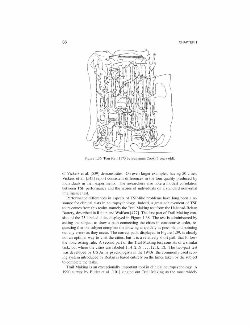
Some of the themes studied by van Rooij et al. can be seen in the tours illustrated in Figures 1.36 and 1.37. The example is a 1,173-city problem from the TSPLIB. The tours were drawn by the same child, first as a 7-year-old and then six years later as a teenager.

THE TSP IN NEUROSCIENCE

Examples of the TSP that are either very small or constructed with a large convex-hull border are routinely solved by humans, with little variation among study par­ticipants. Individual differences in performance quickly arise, however, when gen­eral problem instances have 20 or more cities, as the fashion designer in the study

36 CHAPTER 1

Figure 1.36 Tour for fl1173 by Benjamin Cook (7 years old).

of Vickers et al. [539] demonstrates. On even larger examples, having 50 cities, Vickers et al. [543] report consistent differences in the tour quality produced by individuals in their experiments. The researchers also note a modest correlation between TSP performance and the scores of individuals on a standard nonverbal intelligence test.

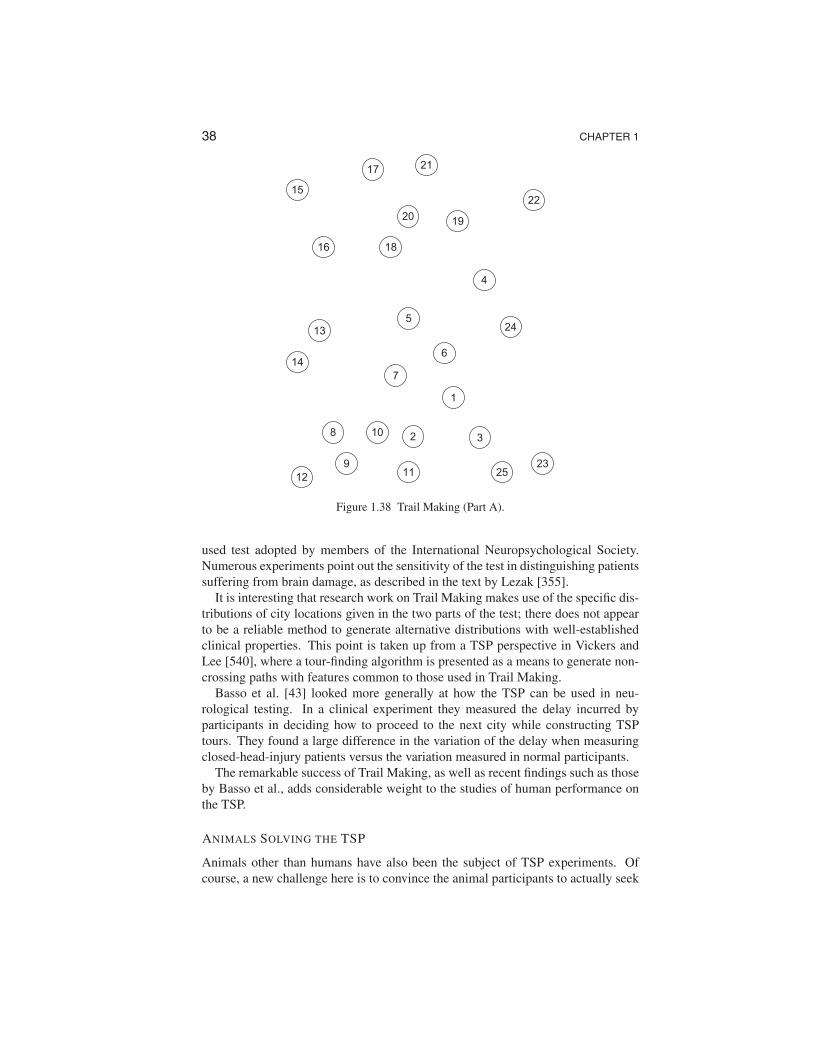
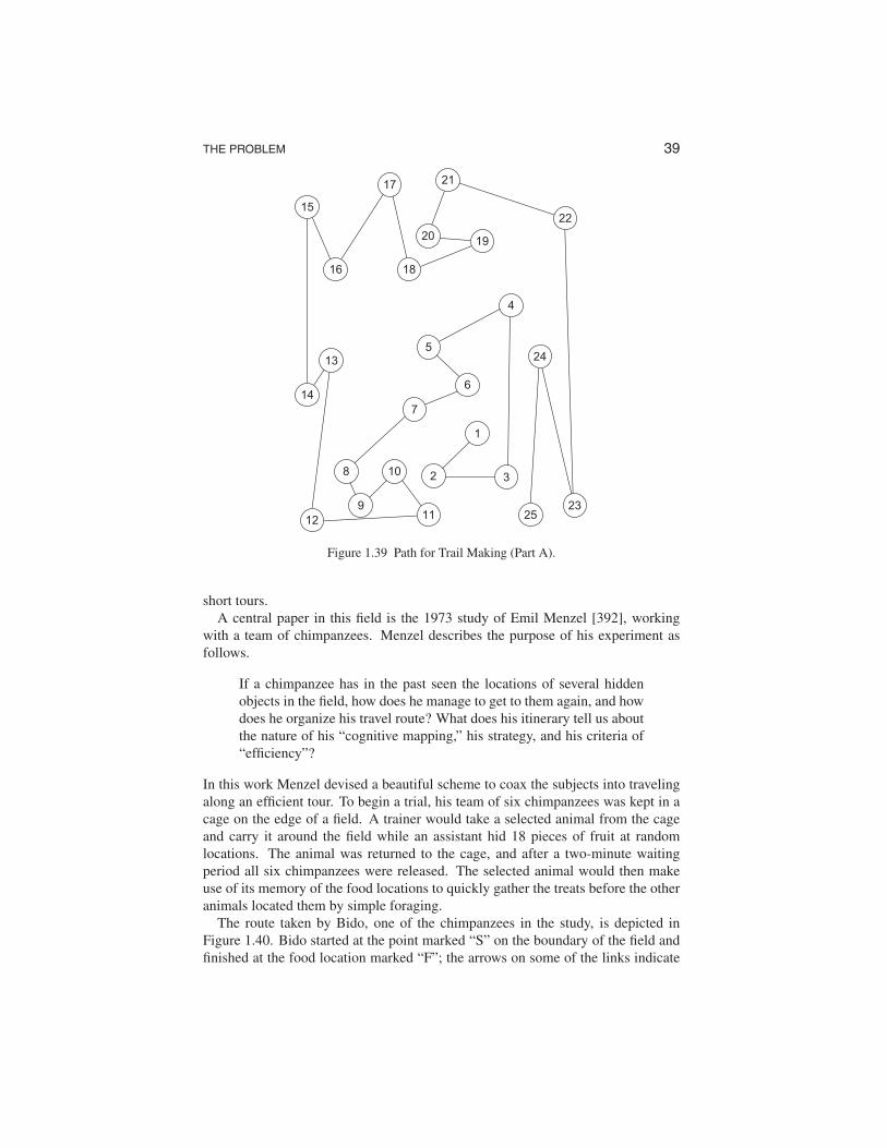
Performance differences in aspects of TSP-like problems have long been a re­source for clinical tests in neuropsychology. Indeed, a great achievement of TSP tours comes from this realm, namely the Trail Making test from the Halstead-Reitan Battery, described in Reitan and Wolfson [477]. The first part of Trail Making con­sists of the 25 labeled cities displayed in Figure 1.38. The test is administered by asking the subject to draw a path connecting the cities in consecutive order, re­questing that the subject complete the drawing as quickly as possible and pointing out any errors as they occur. The correct path, displayed in Figure 1.39, is clearly not an optimal way to visit the cities, but it is a relatively short path that follows the noncrossing rule. A second part of the Trail Making test consists of a similar task, but where the cities are labeled 1, A, 2, B, . . . , 12, L, 13. The two-part test was developed by US Army psychologists in the 1940s; the commonly used scor­ing system introduced by Reitan is based entirely on the times taken by the subject to complete the tasks.

Trail Making is an exceptionally important tool in clinical neuropsychology. A 1990 survey by Butler et al. [101] singled out Trail Making as the most widely

37 THE PROBLEM

Figure 1.37 Tour for fl1173 by Benjamin Cook (13 years old).

38 CHAPTER 1

1

2 3

5

7

108

239 251112

14

17

18

1920

21

22

4

6

16

15

13 24

Figure 1.38 Trail Making (Part A).

used test adopted by members of the International Neuropsychological Society. Numerous experiments point out the sensitivity of the test in distinguishing patients suffering from brain damage, as described in the text by Lezak [355].

It is interesting that research work on Trail Making makes use of the specific dis­tributions of city locations given in the two parts of the test; there does not appear to be a reliable method to generate alternative distributions with well-established clinical properties. This point is taken up from a TSP perspective in Vickers and Lee [540], where a tour-finding algorithm is presented as a means to generate non-crossing paths with features common to those used in Trail Making.

Basso et al. [43] looked more generally at how the TSP can be used in neu­rological testing. In a clinical experiment they measured the delay incurred by participants in deciding how to proceed to the next city while constructing TSP tours. They found a large difference in the variation of the delay when measuring closed-head-injury patients versus the variation measured in normal participants.

The remarkable success of Trail Making, as well as recent findings such as those by Basso et al., adds considerable weight to the studies of human performance on the TSP.

ANIMALS SOLVING THE TSP

Animals other than humans have also been the subject of TSP experiments. Of course, a new challenge here is to convince the animal participants to actually seek

39 THE PROBLEM

1

2 3

5

7

108

239 251112

14

17

18

1920

21

22

4

6

16

15

13 24

Figure 1.39 Path for Trail Making (Part A).

short tours. A central paper in this field is the 1973 study of Emil Menzel [392], working

with a team of chimpanzees. Menzel describes the purpose of his experiment as follows.

If a chimpanzee has in the past seen the locations of several hidden objects in the field, how does he manage to get to them again, and how does he organize his travel route? What does his itinerary tell us about the nature of his “cognitive mapping,” his strategy, and his criteria of “efficiency”?

In this work Menzel devised a beautiful scheme to coax the subjects into traveling along an efficient tour. To begin a trial, his team of six chimpanzees was kept in a cage on the edge of a field. A trainer would take a selected animal from the cage and carry it around the field while an assistant hid 18 pieces of fruit at random locations. The animal was returned to the cage, and after a two-minute waiting period all six chimpanzees were released. The selected animal would then make use of its memory of the food locations to quickly gather the treats before the other animals located them by simple foraging.

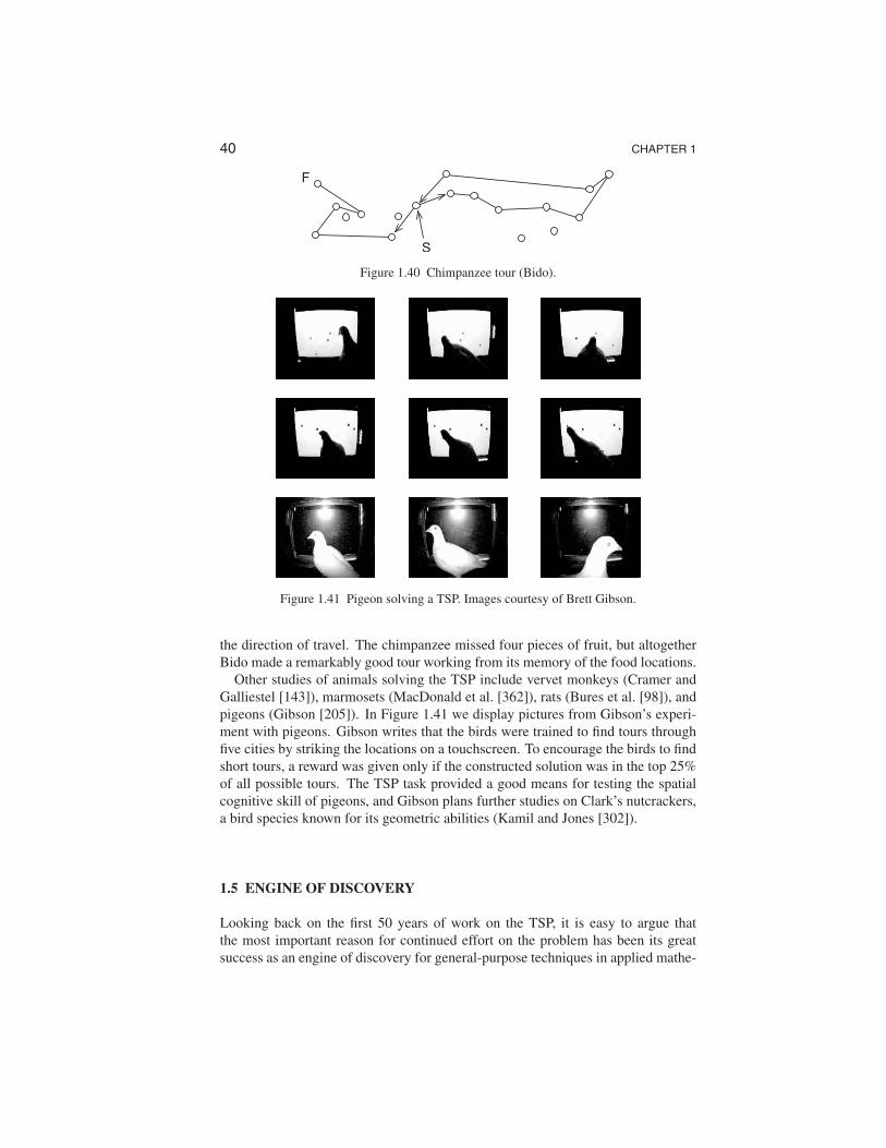
The route taken by Bido, one of the chimpanzees in the study, is depicted in Figure 1.40. Bido started at the point marked “S” on the boundary of the field and finished at the food location marked “F”; the arrows on some of the links indicate

40 CHAPTER 1

S

F

Figure 1.40 Chimpanzee tour (Bido).

Figure 1.41 Pigeon solving a TSP. Images courtesy of Brett Gibson.

the direction of travel. The chimpanzee missed four pieces of fruit, but altogether Bido made a remarkably good tour working from its memory of the food locations.

Other studies of animals solving the TSP include vervet monkeys (Cramer and Galliestel [143]), marmosets (MacDonald et al. [362]), rats (Bures et al. [98]), and pigeons (Gibson [205]). In Figure 1.41 we display pictures from Gibson’s experi­ment with pigeons. Gibson writes that the birds were trained to find tours through five cities by striking the locations on a touchscreen. To encourage the birds to find short tours, a reward was given only if the constructed solution was in the top 25% of all possible tours. The TSP task provided a good means for testing the spatial cognitive skill of pigeons, and Gibson plans further studies on Clark’s nutcrackers, a bird species known for its geometric abilities (Kamil and Jones [302]).

1.5 ENGINE OF DISCOVERY

Looking back on the first 50 years of work on the TSP, it is easy to argue that the most important reason for continued effort on the problem has been its great success as an engine of discovery for general-purpose techniques in applied mathe­

41 THE PROBLEM

matics. We discuss below a few of the many areas to which TSP research has made fundamental contributions.

MIXED-INTEGER PROGRAMMING

One of the major accomplishments of the study of the TSP has been the aid it has given to the development of the flourishing field of mixed-integer program­ming or MIP. An MIP model is a linear programming problem with the additional constraint that some of the variables are required to take on integer values. This ex­tension allows MIP to capture problems where discrete choices are involved, thus greatly increasing its reach over linear programming alone. In the 50 years since its introduction, MIP has become one of the most important models in applied math­ematics, with applications spanning nearly every industry. An illustration of the widespread use of the model is the fact that licenses for commercial MIP solvers currently number in the tens of thousands.

The subject of mixed-integer programming has its roots in the Dantzig, Fulk­erson, and Johnson [151] paper, and nearly every successful solution method for MIP was introduced and studied first in the context of the TSP. Much of the book deals with aspects of this field, and in several chapters we discuss direct contribu­tions to MIP solution methods made through the development of the Concorde TSP code. General treatments of mixed-integer programming can be found in the texts by Schrijver [494], Nemhauser and Wolsey [428], and Wolsey [559].

BRANCH-AND-BOUND METHOD

The well-known branch-and-bound search method has its origins in work on the TSP. The name was introduced in a 1963 TSP paper by Little, Murty, Sweeney, and Karel [360] and the concept was introduced in TSP papers from the 1950s by Bock [69], Croes [145], Eastman [159], and Rossman and Twery [488].

Branch-and-bound is an organized way to make an exhaustive search for the best solution in a specified set. Each branching step splits the search space into two or more subsets in an attempt to create subproblems that may be easier than the original. For example, suppose we have a TSP through a collection of cities in the United States. In this case, if it is not clear whether or not we should travel directly between Philadelphia and New York, then we could split the set of all tours into those that use this edge and and those that do not. By repeatedly making such branching steps we create a collection of subproblems that need to be solved, each defined by a subset of tours that include certain edges and exclude certain others.

Before searching a subproblem and possibly splitting it further, a bound is com­puted on the cost of tours in its subset. In our example, a simple bound is the sum of the travel costs for all edges that we have insisted be in the tours; much better bounds are available, but we do not want to go into the details here. The purpose of the bounding step is to attempt to avoid a fruitless search of a subproblem that contains no solution better than those we have already discovered. The idea is that if the bound is greater than or equal to the cost of a tour we have already found, then we can discard the subproblem without any danger of missing a better tour.

Branch-and-bound is discussed further in Section 4.1. General treatments of

42 CHAPTER 1

branch-and-bound search can be found in books by Brusco and Stahl [97] and Chen and Bushnell [115].

HEURISTIC SEARCH

The TSP has played a role in the development of many of the most widely used paradigms for heuristic-search algorithms. Such algorithms are designed to run quickly and to return a hopefully good solution to a given problem. This theme does not directly match the TSP, which asks for the best possible tour, but the problem has nonetheless served as a basic model for developing and testing ideas in this important area. In this context, researchers look for methods that can detect high-quality tours while using only a modest amount of computational resources. Several of the techniques that have arisen from this work are the following.

• The general class of local-search algorithms has its roots in TSP papers from the 1950s by Morton and Land [403], Flood [182], Bock [69], and Croes [145]. These heuristics take as input an approximate solution to a problem and attempt to iteratively improve it by moving to new solutions that are in some sense close to the original. The basic ingredient is the notion of a “neighborhood” that implicitly defines the list of candidates that can be considered in a given iteration. A nice discussion of these algorithms can be found in the book by Aarts and Lenstra [1].

• The paper of Kirkpatrick, Gelatt, and Vecchi [316] that introduced the simu­lated annealing paradigm worked with the TSP, reporting on heuristic tours for a 400-city problem. A typical local-search algorithm follows the hill-climbing strategy of only moving to a neighboring solution if it is better than the one we have currently. In simulated annealing heuristics, this is relaxed to allow the algorithm to accept with a certain probability a neighbor that is worse than the current solution. At the start of the algorithm the probability of acceptance is high, but it is gradually decreased as the run progresses. The idea is to allow the algorithm to jump over to a better hill before switching to a steady climb. Kirkpatrick et al. write that the motivation comes from a connection with statistical mechanics, where annealing is the process of heat­ing a material and then allowing it to slowly cool to obtain a ground state of minimal energy. A detailed discussion of simulated annealing can be found in the book of van Laarhoven and Aarts [330].

• Neural network algorithms follow a computational paradigm that is based on models of how the brain processes information. The basic components of a neural network are large numbers of simple computing units that com­municate via a network of connections, simulating the parallel operation of neurons in the brain. The TSP was used as a primary example in the classic work of Hopfield and Tank [271] that introduced optimizational aspects of this model.

• Genetic algorithms work with a population of solutions that are combined and modified to produce new solutions, the best of which are selected for the

43 THE PROBLEM

4

52

3 1

0 6

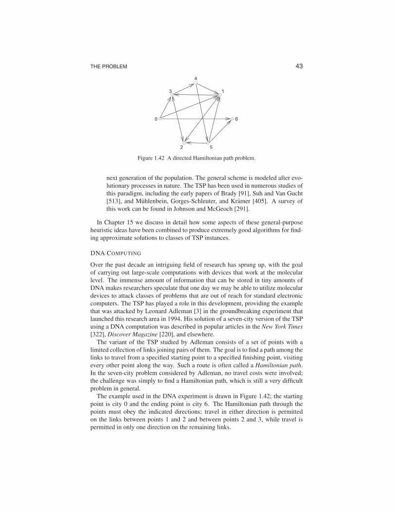
Figure 1.42 A directed Hamiltonian path problem.

next generation of the population. The general scheme is modeled after evo­lutionary processes in nature. The TSP has been used in numerous studies of this paradigm, including the early papers of Brady [91], Suh and Van Gucht [513], and Muhlenbein, Gorges-Schleuter, and Kramer [405]. A survey of this work can be found in Johnson and McGeoch [291].

In Chapter 15 we discuss in detail how some aspects of these general-purpose heuristic ideas have been combined to produce extremely good algorithms for find­ing approximate solutions to classes of TSP instances.

DNA COMPUTING

Over the past decade an intriguing field of research has sprung up, with the goal of carrying out large-scale computations with devices that work at the molecular level. The immense amount of information that can be stored in tiny amounts of DNA makes researchers speculate that one day we may be able to utilize molecular devices to attack classes of problems that are out of reach for standard electronic computers. The TSP has played a role in this development, providing the example that was attacked by Leonard Adleman [3] in the groundbreaking experiment that launched this research area in 1994. His solution of a seven-city version of the TSP using a DNA computation was described in popular articles in the New York Times [322], Discover Magazine [220], and elsewhere.

The variant of the TSP studied by Adleman consists of a set of points with a limited collection of links joining pairs of them. The goal is to find a path among the links to travel from a specified starting point to a specified finishing point, visiting every other point along the way. Such a route is often called a Hamiltonian path. In the seven-city problem considered by Adleman, no travel costs were involved; the challenge was simply to find a Hamiltonian path, which is still a very difficult problem in general.

The example used in the DNA experiment is drawn in Figure 1.42; the starting point is city 0 and the ending point is city 6. The Hamiltonian path through the points must obey the indicated directions; travel in either direction is permitted on the links between points 1 and 2 and between points 2 and 3, while travel is permitted in only one direction on the remaining links.

44 CHAPTER 1

Adleman created a molecular encoding of the problem by assigning each of the seven points to a random string of 20 DNA letters. For example, point 2 was as­signed to

TATCGGATCG GTATATCCGA |and point 3 was assigned to

GCTATTCGAG CTTAAAGCTA. |By considering the 20-letter tags for the points as the combination of two 10-letter tags, a link directed from point a to point b is represented by the string consisting of the second half of the tag for point a and the first half of the tag for point b. For example, a link from point 2 to point 3 would be

GTATATCCGA GCTATTCGAG. |The only exceptions to this rule are links involving the starting and ending cities, 0 and 6, where the entire 20-letter tag is used for these points rather than just the first or second half. To capture the links where travel along either direction is possible, a pair of links is created, one in each direction. In the experiment, many copies of the DNA for the points and links were produced in the laboratory.

The next step in Adleman’s approach is to provide a mechanism for joining links together into a path. To this end, for each point other than 0 and 6, the comple­mentary DNA sequence for the tag is created. Such sequences act as “splints” to pair up links in their proper orientation. For example, the complementary sequence for point 3 could serve to join the links (2, 3) and (3, 4), since the first half of the sequence would pair up with the second half of the encoding of (2, 3) and the second half of the sequence would pair up with the first half of the encoding of (3, 4). Adding many copies of these splints, the mixture is able to generate double-stranded DNA that corresponds to paths in the problem. After careful work in the laboratory over a seven-day period, a double-strand yielding a Hamiltonian path was identified.

This method clearly is not suitable for large examples of the TSP, since the amount of required DNA components grows very rapidly with the number of cities (all paths in the problem are created in the experiment, not just a Hamiltonian path). But this fascinating solution technique is being explored in many directions to de­velop methods suitable for attacking other classes of difficult of problems. As in other cases, the simple nature of the TSP allowed it to play a leading role in the creation of a new computational paradigm. Surveys of work on DNA-based com­puting can be found in Lipton [359], Paun et al. [457], and Amos et al. [11].

1.6 IS THE TSP HARD?

When a description of the TSP appears in a popular setting, it is usually accompa­nied by a short statement of the notorious difficulty of the problem. Is it the case, however, that the TSP is actually hard to solve? The truth is that we do not really know.

45 THE PROBLEM

In Menger’s presentation of the Botenproblem he made the following comments on the complexity of possible solution methods [389], translated from the German original.

This problem can naturally be solved using a finite number of trials. Rules which reduce the number of trials below the number of permu­tations of the given point set are not known. The rule that one should go from the starting point to the next nearest point, then to the next nearest point, and so on, does not always produce the shortest path.

So Menger observed that it is possible to solve the TSP by simply checking each tour, one after another, and choosing the cheapest. He immediately calls for better solution methods, however, not being satisfied with a technique that is finite but clearly impractical.

The notion of a “better than finite” solution method is a subtle concept and is not considered in the usual settings of classical mathematics. Hints of the subject appear in other TSP works, including the following statement in Flood’s 1956 paper [182].

It seems very likely that quite a different approach from any yet used may be required for successful treatment of the problem. In fact, there may well be no general method for treating the problem and impossi­bility results would also be valuable.

In 1964 Gilmore and Gomory wrote a paper [206] with the title “A solvable case of the traveling salesman problem,” clearly implying that the simple algorithm of enumerating all tours is not a feasible solution method.

To put the issue of efficiency in mathematical terms, let us make a rough esti­mate of the running time for the “finite number of trials” algorithm mentioned by Menger. In computing the estimate we follow standard practice and count the num­ber of elementary steps that are required when the algorithm is presented with an n-city TSP as input. This notion can be formalized using Turing machines or other models of computation. Excellent treatments of this subject can be found in books by Aho, Hopcroft, and Ullman [5] and Garey and Johnson [200].

There are many ways to implement a process to enumerate and check all tours; an easy-to-read discussion can be found in Jon Bentley’s article [57] in Unix Review. Good implementations of the process all run in time that is proportional to the total number of tours. To count this number for an n-city TSP is an easy matter. Given a tour, we can choose any point as the starting city. Now from the start we have n −1 choices for the second city, n − 2 choices for the third city, and so on. Multiplying these together we have that the total number of tours is equal to

(n − 1)! = (n − 1) (n − 2) (n − 3) 3 2 1.· · · · · · ·So the direct method suggested by Menger would take time proportional to (n−1)! to solve an n-city TSP.

The simple finite trials method is easy to compare with other possible algorithms for the TSP, since its running-time estimate is the same no matter what n-city in­stance of the TSP is solved. More complicated algorithms, including some of Bent­ley’s [57] variants of the finite trials scheme, do not share this property. In many

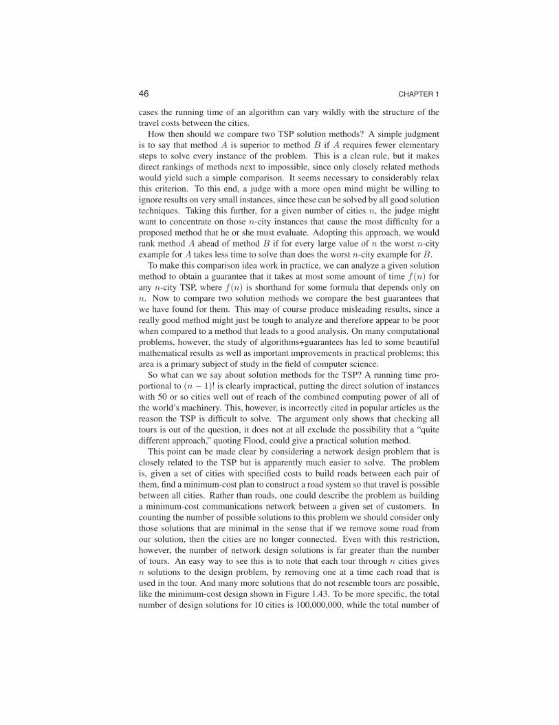
46 CHAPTER 1

cases the running time of an algorithm can vary wildly with the structure of the travel costs between the cities.

How then should we compare two TSP solution methods? A simple judgment is to say that method A is superior to method B if A requires fewer elementary steps to solve every instance of the problem. This is a clean rule, but it makes direct rankings of methods next to impossible, since only closely related methods would yield such a simple comparison. It seems necessary to considerably relax this criterion. To this end, a judge with a more open mind might be willing to ignore results on very small instances, since these can be solved by all good solution techniques. Taking this further, for a given number of cities n, the judge might want to concentrate on those n-city instances that cause the most difficulty for a proposed method that he or she must evaluate. Adopting this approach, we would rank method A ahead of method B if for every large value of n the worst n-city example for A takes less time to solve than does the worst n-city example for B.

To make this comparison idea work in practice, we can analyze a given solution method to obtain a guarantee that it takes at most some amount of time f(n) for any n-city TSP, where f(n) is shorthand for some formula that depends only on n. Now to compare two solution methods we compare the best guarantees that we have found for them. This may of course produce misleading results, since a really good method might just be tough to analyze and therefore appear to be poor when compared to a method that leads to a good analysis. On many computational problems, however, the study of algorithms+guarantees has led to some beautiful mathematical results as well as important improvements in practical problems; this area is a primary subject of study in the field of computer science.

So what can we say about solution methods for the TSP? A running time pro­portional to (n − 1)! is clearly impractical, putting the direct solution of instances with 50 or so cities well out of reach of the combined computing power of all of the world’s machinery. This, however, is incorrectly cited in popular articles as the reason the TSP is difficult to solve. The argument only shows that checking all tours is out of the question, it does not at all exclude the possibility that a “quite different approach,” quoting Flood, could give a practical solution method.

This point can be made clear by considering a network design problem that is closely related to the TSP but is apparently much easier to solve. The problem is, given a set of cities with specified costs to build roads between each pair of them, find a minimum-cost plan to construct a road system so that travel is possible between all cities. Rather than roads, one could describe the problem as building a minimum-cost communications network between a given set of customers. In counting the number of possible solutions to this problem we should consider only those solutions that are minimal in the sense that if we remove some road from our solution, then the cities are no longer connected. Even with this restriction, however, the number of network design solutions is far greater than the number of tours. An easy way to see this is to note that each tour through n cities gives n solutions to the design problem, by removing one at a time each road that is used in the tour. And many more solutions that do not resemble tours are possible, like the minimum-cost design shown in Figure 1.43. To be more specific, the total number of design solutions for 10 cities is 100,000,000, while the total number of

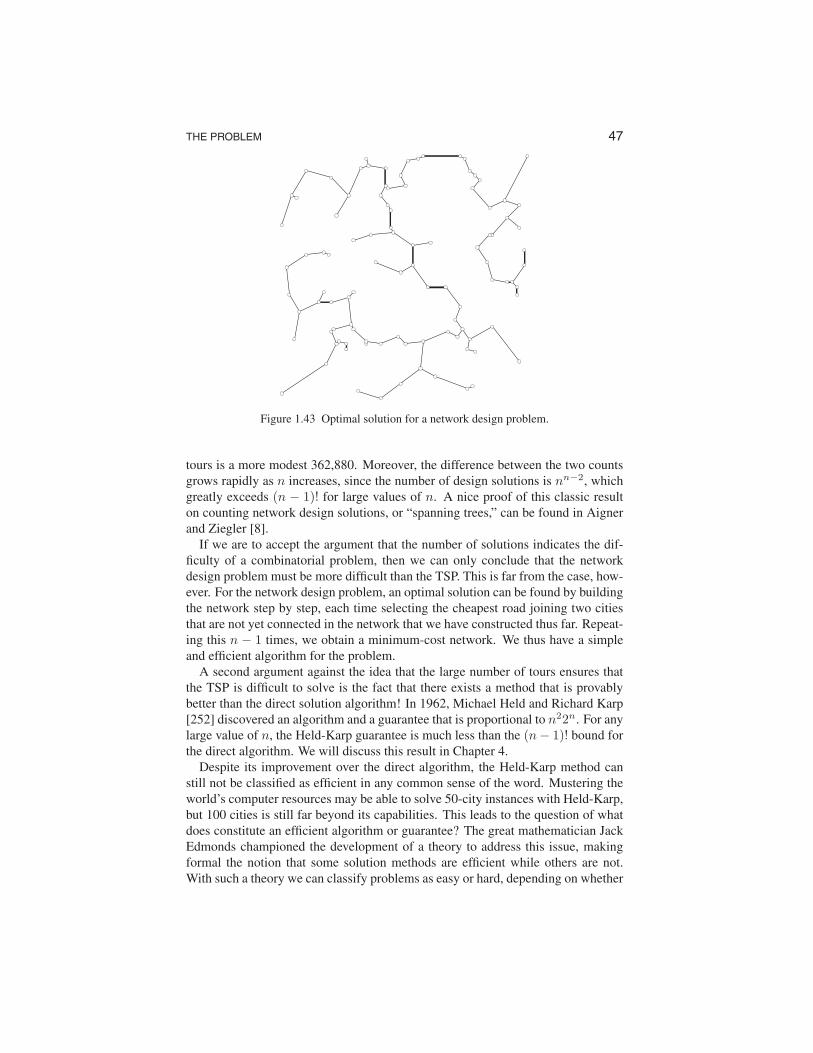
47 THE PROBLEM

Figure 1.43 Optimal solution for a network design problem.

tours is a more modest 362,880. Moreover, the difference between the two counts grows rapidly as n increases, since the number of design solutions is nn−2, which greatly exceeds (n − 1)! for large values of n. A nice proof of this classic result on counting network design solutions, or “spanning trees,” can be found in Aigner and Ziegler [8].

If we are to accept the argument that the number of solutions indicates the dif­ficulty of a combinatorial problem, then we can only conclude that the network design problem must be more difficult than the TSP. This is far from the case, how­ever. For the network design problem, an optimal solution can be found by building the network step by step, each time selecting the cheapest road joining two cities that are not yet connected in the network that we have constructed thus far. Repeat­ing this n − 1 times, we obtain a minimum-cost network. We thus have a simple and efficient algorithm for the problem.

A second argument against the idea that the large number of tours ensures that the TSP is difficult to solve is the fact that there exists a method that is provably better than the direct solution algorithm! In 1962, Michael Held and Richard Karp [252] discovered an algorithm and a guarantee that is proportional to n22n. For any large value of n, the Held-Karp guarantee is much less than the (n − 1)! bound for the direct algorithm. We will discuss this result in Chapter 4.

Despite its improvement over the direct algorithm, the Held-Karp method can still not be classified as efficient in any common sense of the word. Mustering the world’s computer resources may be able to solve 50-city instances with Held-Karp, but 100 cities is still far beyond its capabilities. This leads to the question of what does constitute an efficient algorithm or guarantee? The great mathematician Jack Edmonds championed the development of a theory to address this issue, making formal the notion that some solution methods are efficient while others are not. With such a theory we can classify problems as easy or hard, depending on whether

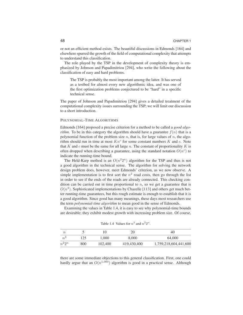
48 CHAPTER 1

or not an efficient method exists. The beautiful discussions in Edmonds [164] and elsewhere spurred the growth of the field of computational complexity that attempts to understand this classification.

The role played by the TSP in the development of complexity theory is em­phasized by Johnson and Papadimitriou [294], who write the following about the classification of easy and hard problems.

The TSP is probably the most important among the latter. It has served as a testbed for almost every new algorithmic idea, and was one of the first optimization problems conjectured to be “hard” in a specific technical sense.

The paper of Johnson and Papadimitriou [294] gives a detailed treatment of the computational complexity issues surrounding the TSP; we will limit our discussion to a short introduction.

POLYNOMIAL-TIME ALGORITHMS

Edmonds [164] proposed a precise criterion for a method to be called a good algo­rithm. To be in this category the algorithm should have a guarantee f(n) that is a polynomial function of the problem size n, that is, for large values of n, the algo­rithm should run in time at most Knc for some constant numbers K and c. Note that K and c must be the same for all large n. The constant of proportionality K is often dropped when describing a guarantee, using the standard notation O(nc) to indicate the running-time bound.

The Held-Karp method is an O(n22n) algorithm for the TSP and thus is not a good algorithm in the technical sense. The algorithm for solving the network design problem does, however, meet Edmonds’ criterion, as we now observe. A simple implementation is to first sort the n2 road costs, then go through the list in order to see if the ends of the roads are already connected. This checking con­dition can be carried out in time proportional to n, so we get a guarantee that is O(n3). Sophisticated implementations by Chazelle [113] and others get much bet­ter running-time guarantees, but this rough estimate is enough to establish that it is a good algorithm. Since good has many meanings, these days most researchers use the term polynomial-time algorithm to mean good in the sense of Edmonds.

Examining the values in Table 1.4, it is easy to see why polynomial-time bounds are desirable; they exhibit modest growth with increasing problem size. Of course,

Table 1.4 Values for n 3 and n 22n .

n 5 10 20 40

n3 125 1,000 8,000 64,000

n22n 800 102,400 419,430,400 1,759,218,604,441,600

there are some immediate objections to this general classification. First, one could hardly argue that an O(n1,000) algorithm is good in a practical sense. Although

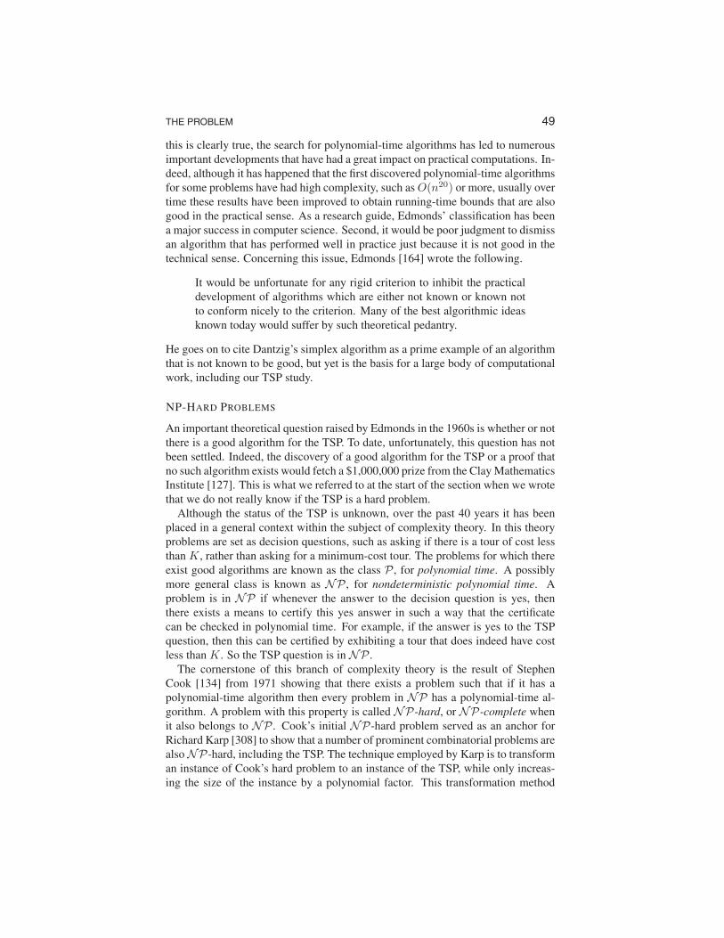
49 THE PROBLEM

this is clearly true, the search for polynomial-time algorithms has led to numerous important developments that have had a great impact on practical computations. In­deed, although it has happened that the first discovered polynomial-time algorithms for some problems have had high complexity, such as O(n20) or more, usually over time these results have been improved to obtain running-time bounds that are also good in the practical sense. As a research guide, Edmonds’ classification has been a major success in computer science. Second, it would be poor judgment to dismiss an algorithm that has performed well in practice just because it is not good in the technical sense. Concerning this issue, Edmonds [164] wrote the following.

It would be unfortunate for any rigid criterion to inhibit the practical development of algorithms which are either not known or known not to conform nicely to the criterion. Many of the best algorithmic ideas known today would suffer by such theoretical pedantry.

He goes on to cite Dantzig’s simplex algorithm as a prime example of an algorithm that is not known to be good, but yet is the basis for a large body of computational work, including our TSP study.

NP-HARD PROBLEMS

An important theoretical question raised by Edmonds in the 1960s is whether or not there is a good algorithm for the TSP. To date, unfortunately, this question has not been settled. Indeed, the discovery of a good algorithm for the TSP or a proof that no such algorithm exists would fetch a $1,000,000 prize from the Clay Mathematics Institute [127]. This is what we referred to at the start of the section when we wrote that we do not really know if the TSP is a hard problem.

Although the status of the TSP is unknown, over the past 40 years it has been placed in a general context within the subject of complexity theory. In this theory problems are set as decision questions, such as asking if there is a tour of cost less than K, rather than asking for a minimum-cost tour. The problems for which there exist good algorithms are known as the class P , for polynomial time. A possibly more general class is known as NP , for nondeterministic polynomial time. A problem is in NP if whenever the answer to the decision question is yes, then there exists a means to certify this yes answer in such a way that the certificate can be checked in polynomial time. For example, if the answer is yes to the TSP question, then this can be certified by exhibiting a tour that does indeed have cost less than K. So the TSP question is in NP .

The cornerstone of this branch of complexity theory is the result of Stephen Cook [134] from 1971 showing that there exists a problem such that if it has a polynomial-time algorithm then every problem in NP has a polynomial-time al­gorithm. A problem with this property is called NP-hard, or NP-complete when it also belongs to NP . Cook’s initial NP-hard problem served as an anchor for Richard Karp [308] to show that a number of prominent combinatorial problems are also NP-hard, including the TSP. The technique employed by Karp is to transform an instance of Cook’s hard problem to an instance of the TSP, while only increas­ing the size of the instance by a polynomial factor. This transformation method

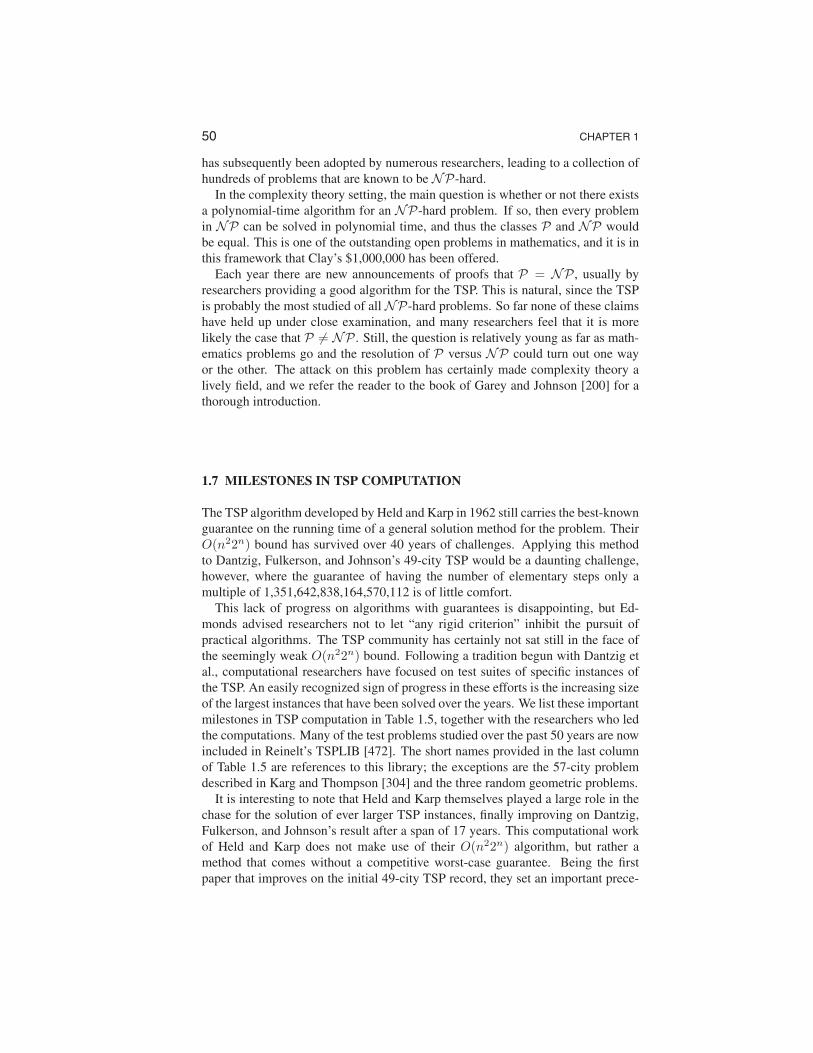
50 CHAPTER 1

has subsequently been adopted by numerous researchers, leading to a collection of hundreds of problems that are known to be NP-hard.

In the complexity theory setting, the main question is whether or not there exists a polynomial-time algorithm for an NP-hard problem. If so, then every problem in NP can be solved in polynomial time, and thus the classes P and NP would be equal. This is one of the outstanding open problems in mathematics, and it is in this framework that Clay’s $1,000,000 has been offered.

Each year there are new announcements of proofs that P = NP , usually by researchers providing a good algorithm for the TSP. This is natural, since the TSP is probably the most studied of all NP-hard problems. So far none of these claims have held up under close examination, and many researchers feel that it is more likely the case that P =� NP . Still, the question is relatively young as far as math­ematics problems go and the resolution of P versus NP could turn out one way or the other. The attack on this problem has certainly made complexity theory a lively field, and we refer the reader to the book of Garey and Johnson [200] for a thorough introduction.

1.7 MILESTONES IN TSP COMPUTATION

The TSP algorithm developed by Held and Karp in 1962 still carries the best-known guarantee on the running time of a general solution method for the problem. Their O(n22n) bound has survived over 40 years of challenges. Applying this method to Dantzig, Fulkerson, and Johnson’s 49-city TSP would be a daunting challenge, however, where the guarantee of having the number of elementary steps only a multiple of 1,351,642,838,164,570,112 is of little comfort.

This lack of progress on algorithms with guarantees is disappointing, but Ed­monds advised researchers not to let “any rigid criterion” inhibit the pursuit of practical algorithms. The TSP community has certainly not sat still in the face of the seemingly weak O(n22n) bound. Following a tradition begun with Dantzig et al., computational researchers have focused on test suites of specific instances of the TSP. An easily recognized sign of progress in these efforts is the increasing size of the largest instances that have been solved over the years. We list these important milestones in TSP computation in Table 1.5, together with the researchers who led the computations. Many of the test problems studied over the past 50 years are now included in Reinelt’s TSPLIB [472]. The short names provided in the last column of Table 1.5 are references to this library; the exceptions are the 57-city problem described in Karg and Thompson [304] and the three random geometric problems.

It is interesting to note that Held and Karp themselves played a large role in the chase for the solution of ever larger TSP instances, finally improving on Dantzig, Fulkerson, and Johnson’s result after a span of 17 years. This computational work of Held and Karp does not make use of their O(n22n) algorithm, but rather a method that comes without a competitive worst-case guarantee. Being the first paper that improves on the initial 49-city TSP record, they set an important prece­

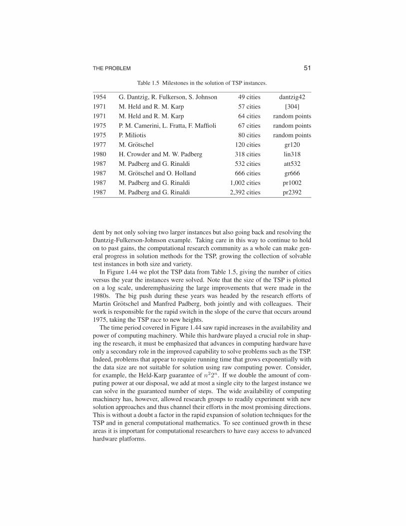
51 THE PROBLEM

Table 1.5 Milestones in the solution of TSP instances.

1954 G. Dantzig, R. Fulkerson, S. Johnson 49 cities dantzig42

1971 M. Held and R. M. Karp 57 cities [304]

1971 M. Held and R. M. Karp 64 cities random points

1975 P. M. Camerini, L. Fratta, F. Maffioli 67 cities random points

1975 P. Miliotis 80 cities random points

1977 M. Grotschel 120 cities gr120

1980 H. Crowder and M. W. Padberg 318 cities lin318

1987 M. Padberg and G. Rinaldi 532 cities att532

1987 M. Gr¨ 666 cities otschel and O. Holland gr666

1987 M. Padberg and G. Rinaldi 1,002 cities pr1002

1987 M. Padberg and G. Rinaldi 2,392 cities pr2392

dent by not only solving two larger instances but also going back and resolving the Dantzig-Fulkerson-Johnson example. Taking care in this way to continue to hold on to past gains, the computational research community as a whole can make gen­eral progress in solution methods for the TSP, growing the collection of solvable test instances in both size and variety.

In Figure 1.44 we plot the TSP data from Table 1.5, giving the number of cities versus the year the instances were solved. Note that the size of the TSP is plotted on a log scale, underemphasizing the large improvements that were made in the 1980s. The big push during these years was headed by the research efforts of Martin Grotschel and Manfred Padberg, both jointly and with colleagues. Their work is responsible for the rapid switch in the slope of the curve that occurs around 1975, taking the TSP race to new heights.

The time period covered in Figure 1.44 saw rapid increases in the availability and power of computing machinery. While this hardware played a crucial role in shap­ing the research, it must be emphasized that advances in computing hardware have only a secondary role in the improved capability to solve problems such as the TSP. Indeed, problems that appear to require running time that grows exponentially with the data size are not suitable for solution using raw computing power. Consider, for example, the Held-Karp guarantee of n22n . If we double the amount of com­puting power at our disposal, we add at most a single city to the largest instance we can solve in the guaranteed number of steps. The wide availability of computing machinery has, however, allowed research groups to readily experiment with new solution approaches and thus channel their efforts in the most promising directions. This is without a doubt a factor in the rapid expansion of solution techniques for the TSP and in general computational mathematics. To see continued growth in these areas it is important for computational researchers to have easy access to advanced hardware platforms.

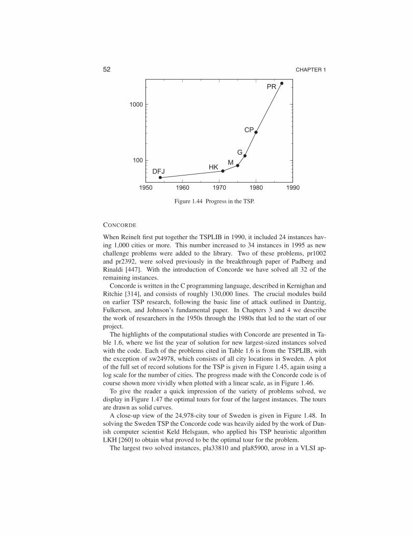
52 CHAPTER 1

100

1000

DFJ HK

M

G

CP

PR

1950 1960 1970 1980 1990

Figure 1.44 Progress in the TSP.

CONCORDE

When Reinelt first put together the TSPLIB in 1990, it included 24 instances hav­ing 1,000 cities or more. This number increased to 34 instances in 1995 as new challenge problems were added to the library. Two of these problems, pr1002 and pr2392, were solved previously in the breakthrough paper of Padberg and Rinaldi [447]. With the introduction of Concorde we have solved all 32 of the remaining instances.

Concorde is written in the C programming language, described in Kernighan and Ritchie [314], and consists of roughly 130,000 lines. The crucial modules build on earlier TSP research, following the basic line of attack outlined in Dantzig, Fulkerson, and Johnson’s fundamental paper. In Chapters 3 and 4 we describe the work of researchers in the 1950s through the 1980s that led to the start of our project.

The highlights of the computational studies with Concorde are presented in Ta­ble 1.6, where we list the year of solution for new largest-sized instances solved with the code. Each of the problems cited in Table 1.6 is from the TSPLIB, with the exception of sw24978, which consists of all city locations in Sweden. A plot of the full set of record solutions for the TSP is given in Figure 1.45, again using a log scale for the number of cities. The progress made with the Concorde code is of course shown more vividly when plotted with a linear scale, as in Figure 1.46.

To give the reader a quick impression of the variety of problems solved, we display in Figure 1.47 the optimal tours for four of the largest instances. The tours are drawn as solid curves.

A close-up view of the 24,978-city tour of Sweden is given in Figure 1.48. In solving the Sweden TSP the Concorde code was heavily aided by the work of Dan­ish computer scientist Keld Helsgaun, who applied his TSP heuristic algorithm LKH [260] to obtain what proved to be the optimal tour for the problem.

The largest two solved instances, pla33810 and pla85900, arose in a VLSI ap­

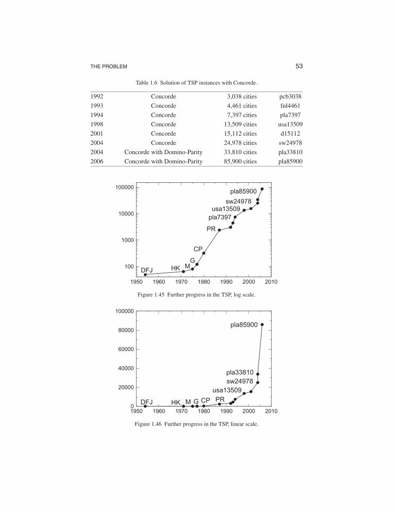
53 THE PROBLEM

Table 1.6 Solution of TSP instances with Concorde.

1992 Concorde 3,038 cities pcb3038

1993 Concorde 4,461 cities fnl4461

1994 Concorde 7,397 cities pla7397

1998 Concorde 13,509 cities usa13509

2001 Concorde 15,112 cities d15112

2004 Concorde 24,978 cities sw24978

2004 Concorde with Domino-Parity 33,810 cities pla33810

2006 Concorde with Domino-Parity 85,900 cities pla85900

100

1000

10000

100000

M G

CP

PR

pla7397

usa13509 sw24978

pla85900

DFJ HK

1950 1960 1970 1980 1990 2000

Figure 1.45 Further progress in the TSP, log scale.

2010

1950 1960 1970 1980 1990 2000

Figure 1.46 Further progress in the TSP, linear scale.

2010 0

20000

40000

60000

80000

100000

sw24978

pla85900

pla33810

DFJ HK GM CP PR

usa13509

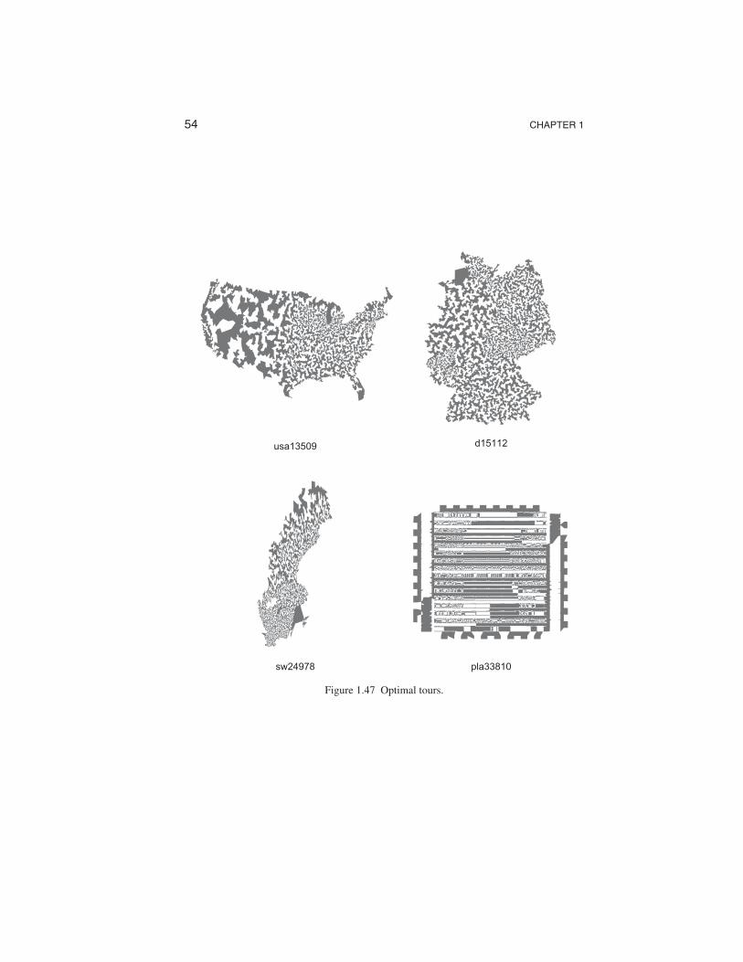
54 CHAPTER 1

usa13509 d15112

sw24978 pla33810

Figure 1.47 Optimal tours.

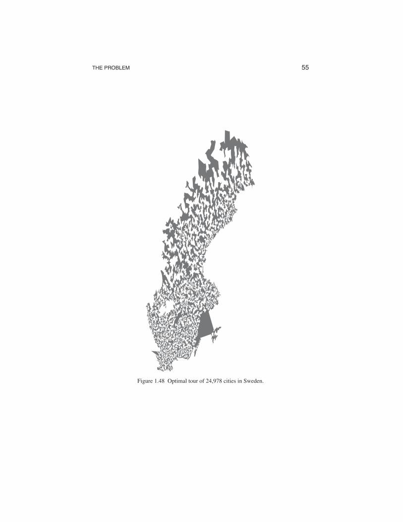
55 THE PROBLEM

Figure 1.48 Optimal tour of 24,978 cities in Sweden.

56 CHAPTER 1

plication that is described in the next chapter. The solution to these problems was accomplished in part by extending the basic Concorde code with new techniques by Cook, Espinoza, and Goycoolea [136], described in Chapter 9. These efforts build on algorithmic work of Letchford [347], and we hope it is a sign of future improvements by other research teams, as Concorde is used as a bridge to bring TSP theory to practical computation.

WORLD TSP

With the solution of the 85,900-city instance, the complete collection of TSPLIB instances has now been solved. This should not signal the end of the line for TSP computation, however. Much more can be learned by pursuing larger and even more difficult instances. To take stock of what may be needed to face the challenge of much larger problems, in 2001 we put together a 1,904,711-city instance of lo­cations throughout the world. The solution of such a TSP is far too difficult for Concorde, but many researchers have taken up the challenge of trying to produce close approximations to an optimal tour. At the time of the writing of this book, the best-known solution has been obtained by Keld Helsgaun with variants of his LKH heuristic code. Remarkably, with lower bounds provided by Concorde, we know that Helsgaun’s tour is no more than 0.058% longer than an optimal world tour. A picture of the tour is given in Figure 1.49. We discuss in Chapter 16 the current attacks on this instance and how Concorde’s solution modules behave when scaled up to problems of this size.

1.8 OUTLINE OF THE BOOK

We mentioned at the outset that the primary goal of this book is to describe the theory and algorithms adopted in the Concorde TSP code. Continuing some of the discussions begun in this chapter, we also cover the history of TSP computation, along with applications of TSP models.

In Chapter 2 we begin with a survey of applications, and follow this in Chapter 3 with a detailed discussion of Dantzig, Fulkerson, and Johnson’s [151] seminal work. The cutting-plane method they created for the solution of the 49-city TSP set the stage for the leaps in performance that were made over the next 50 years. Much of the further development and extension of the Dantzig et al. ideas was led by Martin Grotschel and Manfred Padberg, and we survey this work in Chapter 4.

At the heart of the Concorde TSP code are the implementations of algorithms and techniques for finding cutting planes. The methods that are utilized in these implementations are presented in Chapters 5 through 11.

In Chapter 12 we lay out the steps that were necessary to manage the linear programming problems that need to be solved when applying the cutting-plane method to large-scale TSP instances. We follow this in Chapter 13 with a detailed description of the workings of the ILOG-CPLEX linear programming solver that is the engine for our cutting-plane implementation.

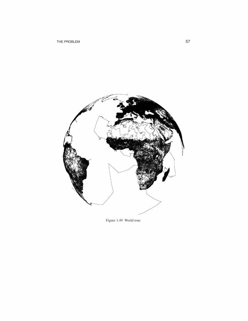
57 THE PROBLEM

Figure 1.49 World tour.

58 CHAPTER 1

The Concorde code uses an enumeration scheme to continue the TSP solution process when cutting planes themselves are no longer making significant progress. The design of this portion of the code is described in Chapter 14. Heuristic al­gorithms for finding tours (a component of the solution process) are presented in Chapter 15.

Results of computational tests with Concorde are given in Chapter 16. We present results on the TSPLIB and World TSP instances, as well as on random Euclidean problems, leading to a study of the Beardwood, Halton, and Hammers-ley [45] TSP constant β.

Finally, in Chapter 17 we discuss some of the research directions various groups have adopted in attempts to push beyond the limits of the TSP approach used in Concorde.