copyright warning &...

Copyright Warning & Restrictions

The copyright law of the United States (Title 17, United States Code) governs the making of photocopies or other

reproductions of copyrighted material.

Under certain conditions specified in the law, libraries and archives are authorized to furnish a photocopy or other

reproduction. One of these specified conditions is that the photocopy or reproduction is not to be “used for any

purpose other than private study, scholarship, or research.” If a, user makes a request for, or later uses, a photocopy or reproduction for purposes in excess of “fair use” that user

may be liable for copyright infringement,

This institution reserves the right to refuse to accept a copying order if, in its judgment, fulfillment of the order

would involve violation of copyright law.

Please Note: The author retains the copyright while the New Jersey Institute of Technology reserves the right to

distribute this thesis or dissertation

Printing note: If you do not wish to print this page, then select “Pages from: first page # to: last page #” on the print dialog screen

The Van Houten library has removed some of the personal information and all signatures from the approval page and biographical sketches of theses and dissertations in order to protect the identity of NJIT graduates and faculty.

ABSTRACT

ARQ PROTOCOL FOR JOINT SOURCE AND CHANNEL CODINGAND ITS APPLICATIONS

byBin He

Shannon's separation theorem states that for transmission over noisy channels,

approaching channel capacity is possible with the separation of source and channel

coding. Practically, the situation is different. Infinite size blocks are needed

to achieve this theoretical limit. Also, time-varying channels require a different

approach. This leads to many approaches for source and channel coding. This

dissertation will address a joint source and channel coding that suits Automatic

Repeat Request (ARQ) application and applies it to packet switching networks.

Following aspects of the proposed joint source and channel coding approach will be

presented:

1. The design of the proposed joint source and channel coding scheme. The

approach is based on a variable length coding scheme which adapts the

arithmetic coding process for joint source and channel coding.

2. The protocol using this joint source and channel coding scheme in commu-

nication systems. The error recovery technique of the proposed scheme is

presented.

3. The application of the scheme and protocol. The design is applied to wireless

TCP network and real-time video transmissions.

The coding scheme embeds the redundancy needed for error detection in source

coding stage. The self-synchronization property of lossless compression is utilized

by decoder to detect channel errors. With this approach, error detection may be

delayed. The delay in detection is referred to as error propagation distance. This

work analyzes the distribution of error propagation distance. The error recovery

technique of this joint source and channel coding for ARQ (JARQ) protocol is

analyzed. Throughput is studied using signal flow graph for both independent

channel and nonindependent channels. A .packet combining technique is presented

which utilizes the non-uniform distribution of error propagation distance to increase

the throughput.

The proposed scheme may be applied to many areas. In particular, two appli-

cations are discussed. A TCP/JARQ protocol stack is introduced and the coordi-

nation between TCP and JARQ layers is discussed to maximize system performance.

By limiting the number of retransmission, the proposed scheme is applied to real-time

transmission to meet timing requirement.

ARQ PROTOCOL FOR JOINT SOURCE AND CHANNEL CODINGAND ITS APPLICATIONS

byBin He

A DissertationSubmitted to the Faculty of

New Jersey Institute of Technologyin Partial Fulfillment of the Requirements for the Degree of

Doctor of Philosophy in Electrical Engineering

Department of Electrical and Computer Engineering

August 2001

APPROVAL PAGE

ARQ Protocol for Joint Source and Channel Coding and ItsApplications

Bin He

Dr. Constantine N. Manikopoulos, Dissertation Advisor DateAssociate Professor of Electrical and Computer Engineering, NJIT

Dr. Yun-Qing Shi, Committee Member DateAssociate Professor of Electrical and Computer Engineering, NJIT

Dr. Symeon Papavassiliou, Committee Member DateAssistant Professor of Electrical and Computer Engineering, NJIT

Dr. Huifang Sun, Committee Member DateDeputy Director, Murray Hill Lab, Mitsubishi Electric Research Laboratories

Dr. George F. Elmasry, Committee Member DateMember of Technical Staff, Lucent Technologies

BIOGRAPHICAL SKETCH

Author: Bin He

Degree: Doctor of Philosophy

Date: August 2001

Undergraduate and Graduate Education:

• Doctor of Philosophy in Electrical Engineering,New Jersey Institute of Technology, Newark, NJ, 2001

• Master of Science in Electrical Engineering,Beijing University of Aeronautics and Astronautics, Beijing, P. R. China, 1997

• Bachelor of Engineering in Electrical Engineering,Beijing University of Aeronautics and Astronautics, Beijing, P. R. China, 1993

Major: Electrical Engineering

Publications and Presentations:

B. He and C. N. Manikopoulos, "Performance analysis of ARQ protocol with delayeddetection for joint source and channel coding," in Proceedings of the 35thAnnual Conference on Information Sciences and Systems, (Baltimore, MD),Mar. 2001.

B. He and C. N. Manikopoulos, "A comparison between two error detectiontechniques using arithmetic coding," in Proceedings of the Data CompressionConference, (Snowbird, Utah), Mar. 2001.

B. He and C. N. Manikopoulos, "An automatic repeat request protocol using jointsource and channel coding," in Proceedings of the CSCC 2000 World Multi-conference, (Athens, Greece), July 2000.

B. He, G. F. Elmasry and C. N. Manikopoulos, "A network protocol for joint lossless-source and channel coding (JARQ) with packet combining," in Proceedings ofthe 34th Annual Conference on Information Sciences and Systems, (Princeton,

NJ), Mar. 2000.

iv

B. He, G. F. Elmasry, C. N. Manikopoulos, and Y.-Q. Shi, "A Go-Back-N + 1protocol and its application in wireless ATM networks," in Proceedings of the33rd Annual Conference on Information Sciences and Systems, (Baltimore,MD), Mar. 1999.

B. He and C. N. Manikopoulos, "Performance of an ARQ protocol based onjoint source and channel coding on nonindependent channel," to appear inProceedings of the IEEE Vehicular Technology Conference (VTC-01/Fall),(Atlantic City, NJ), Oct. 2001.

B. He and C. N. Manikopoulos, "A comparison between two error detectiontechniques using arithmetic coding," to appear in Proceedings of the Inter-national Conference on Computing and Information Technologies, (UpperMontclair, NJ), Oct. 2001.

B. He, G. F. Elmasry and C. N. Manikopoulos, "Joint lossless-source and channelcoding using ARQ/Go-Back-(N, M) for image transmission," submitted toIEEE Trans. Image Processing, 2000.

B. He and C. N. Manikopoulos, "ARQ protocols for joint lossless-source and channelcoding with delayed detection," submitted to IEEE Trans. Commun., 2000.

B. He and C. N. Manikopoulos, "Performance analysis of ARQ protocols for jointlossless-source and channel coding with delayed detection," to be submittedto IEEE Trans. Commun., 2001.

B. He and C. N. Manikopoulos, "Efficient joint source and channel coding ARQprotocol for wireless networks," to be submitted to Electronic Letters, 2001.

This work is dedicated to my beloved family

vi

ACKNOWLEDGMENT

First and foremost, I would like to express my sincere gratitude to my Advisor,

Prof. Manikopoulos. I feel extremely fortunate to have him as my advisor. I am

deeply grateful to him for his valuable suggestions, continuous support and consistent

encouragement. His style of guidance and his creativity made my graduate study a

great experience.

I extend my sincere appreciation to my dissertation committee, Prof. Yun-Qing

Shi, Prof. Symeon Papavassiliou, Dr. Huifang Sun (Murray Hill Lab, Mitsubishi

Electric Research Laboratories) and Dr. George F. Elmasry (General Dynamics

Communication Systems, formerly Lucent Technologies) for their interest in this work

and stimulating discussions and suggestions. I would especially like to acknowledge

Dr. Elmasry for his invaluable support and contribution to my professional devel-

opment.

I have thoroughly enjoyed knowing and working with fellow researchers during

my study. I would like to thank my friends in the department, especially Feihong

Chen, Qiang Peng, Minyi Zhao and Surong Zeng, for their continuous help and

valuable discussions. I also appreciate Ms. Lisa Fitton, wife of Dr. Elmasry, for her

help in revising and editing my paper.

Finally, I would like to express my special gratitude to my family. I am very

grateful to my parents, Taixiang He and Zhaolan Xie, for their endless love and

support. They always have confidence in me. I would like to express my deepest and

special gratitude to my wife and closest friend, Min Tan, who provided continuous

encouragement and brought so much happiness and joy into my life. Words cannot

express the gratitude I feel toward them.

vi'

TABLE OF CONTENTS

Chapter Page

1 INTRODUCTION 1

1.1 Background and Motivation 1

1.2 Organization of the Dissertation 3

2 JOINT SOURCE AND CHANNEL DESIGN WITH VARIABLE LENGTHCODES USING ARITHMETIC CODING 6

2.1 Joint Source and Channel Design 6

2.2 Delay Characteristic Analysis 8

2.2.1 Misdetection Probability and Error Propagation Distance . . . 8

2.2.2 Modeling of Error Propagation PDF 9

2.3 Prevention of Long Propagation Distance 13

2.3.1 Two Types of Error in Arithmetic Coding 13

2.3.2 Experiments 17

2.4 A Comparison Between Two Error Detection Techniques Using Ari-thmetic Coding 19

2.4.1 Forbidden Symbol Approach and Marker Symbol Approach 19

2.4.2 Comparison of Redundancy and Error Propagation Distance 20

2.5 Conclusion 22

3 ERROR RECOVERY PROTOCOL OF THE PROPOSED JOINT SOUR-CE AND CHANNEL DESIGN 24

3.1 Introduction to the JARQ Protocol 25

3.2 Throughput Enhancement with Packet Combining 26

3.3 Summary 28

4 THROUGHPUT ANALYSIS OF JARQ PROTOCOL ON INDEPEN-DENT CHANNEL 29

4.1 Throughput Analysis of Go-Back-(N, M) Protocol 29

4.2 Optimal Case for Go-Back-(N, M) Protocol 32

vii'

TABLE OF CONTENTS(Continued)

Chapter Page

4.3 Throughput of Go-Back-(N, M) Protocol with Packet Combining . . . 33

4.4 Simulation Results 36

4.4.1 Selection of Code Rate for JARQ and Conventional ARQ . . . 36

4.4.2 Throughput Comparison 38

4.5 Summary 39

5 THROUGHPUT ANALYSIS OF JARQ PROTOCOL ON NONINDE-PENDENT CHANNEL 41

5.1 Introduction 41

5.2 Nonindependent Channel Model 42

5.3 Signal Flow Graph of Go-Back-(N, M) Protocol and ThroughputAnalysis 44

5.4 Simulation Results 46

5.4.1 Simulation Results without Packet Combining 46

5.4.2 Simulation Results with Packet Combining 48

5.5 Conclusion 52

6 JARQ APPLICATION TO WIRELESS TCP NETWORKS 53

6.1 Introduction 53

6.2 TCP/RLP Protocol Stack 57

6.3 Simulations 59

6.3.1 Simulation Tools 59

6.3.2 Performance of TCP/JARQ Protocol Stack 61

6.3.3 Performance Comparison of TCP/ARQ and TCP/JARQ Pro-tocols 64

6.4 Summary 67

7 JARQ APPLICATION TO REAL-TIME TRANSMISSION WITH LIMIT-ED NUMBER OF RETRANSMISSION 69

ix

TABLE OF CONTENTS(Continued)

Chapter Page

7.1 Introduction 69

7.2 Three Frame Types in Layered MPEG Application 70

7.3 Delay Analysis of Different Number of Retransmission 72

7.4 Simulations 74

7.5 Conclusion 78

8 CONCLUSIONS AND FUTURE WORK 79

REFERENCES 84

LIST OF FIGURES

Figure Page

2.1 Diagram of the JSCC design 7

2.2 Error propagation distance PDF of text transmission 10

2.3 Error propagation distance PDF of image transmission 10

2.4 Modeling of error propagation PDF for text transmission 12

2.5 Modeling of error propagation PDF for image transmission 13

2.6 Arithmetic decoding algorithm 14

2.7 Illustration of second type of error 15

2.8 Error propagation distance PDF of combined strategy and previousmarker strategy 18

2.9 Comparison of error propagation distances of two approaches 22

3.1 Detection state flow of Go-Back-(N, M) (M >= 1) protocol 25

3.2 Go-Back-(N, M) protocol (M = 1) 26

3.3 Apply packet combining to a frame and its copy 28

4.1 Signal flow graph of Go-Back-N protocol 30

4.2 Signal flow graph of Go-Back-(N, M) protocol 30

4.3 Signal flow graph of Go-Back-(N, M) protocol with packet combining 34

4.4 Relation between ηcomb and a, for given p, s and M. 35

4.5 Packet combining gain 36

4.6 Throughput comparison of Go-Back-(N, M) and Go-Back-N protocols(N = 4 and M = 2) 38

4.7 Throughput comparison of Go-Back-(N, M) and Go-Back-N protocols(N = 64 and M = 2) 39

4.8 Throughput of Go-Back-(N, M) protocol using packet combining (N = 4and M = 2) 40

4.9 Throughput of Go-Back-(N, M) protocol using packet combining (N =64 and M = 2) 40

xi

LIST OF FIGURES(Continued)

Figure Page

5.1 Signal flow graph of Go-Back-(N, M) protocol on nonindependent channel 44

5.2 Comparison of theoretical throughput and simulation result of Go-Back-(N, M) protocol on nonindependent channel (fdT = 0.03) 47

5.3 Throughput comparison of Go-Back-(N, M) protocol on nonindependentchannel and independent channels (F = 5.0 dB and F = 15.0 dB) . . . 48

5.4 Throughput comparison of Go-Back-(N, M) protocol on nonindependentchannel with and without packet combining (combining window sizes = 4. fdT = 0.01, 0.03, and 1.0) 49




5.8 Throughput comparison of Go-Back-(N, M) protocol on nonindependentchannel with and without packet combining (combining window sizes = 4, 10, 20, and 64. F = 5.0 dB) 51

5.9 Throughput comparison of Go-Back-(N, M) protocol on nonindependentchannel with and without packet combining (combining window sizes = 4, 10, 20, and 64. F = 15.0 dB) 52

6.1 TCP state transition diagram. Reprinted from TCP/IP Illustrated,Volume 1: The Protocols by W. Richard Stevens. Copyright © 1994by Addison-Wesley Publishing Company, Inc. 54

6.2 TCP/RLP protocol stack 58

6.3 TCP/JARQ algorithm flow chart 59

6.4 OPNET network model of TCP/RLP simulation 60

6.5 TCP throughput of system without RLP in data link layer 62

X11

LIST OF FIGURES(Continued)

Figure Page

6.6 TCP throughput of system with RLP in data link layer (most correlatedchannel with fdT = 0.01) 62

6.7 TCP throughput of system with RLP in data link layer (correlatedchannel with fdT = 0.1) 63

6.8 TCP throughput of system with RLP in data link layer (less correlatedchannel with fdT = 1.0) 63

6.9 TCP throughput of system with RLP in data link layer (independentchannel) 64

6.10 Comparison of TCP congestion window size cwnd of system without RLPand system with RLP and 1 retransmission attempt 65

6.11 Comparison of TCP congestion window size cwnd of system without RLPand system with RLP and 10 retransmission attempts 65

6.12 Simulation comparison of system using JARQ and conventional ARQschemes 67

7.1 Three MPEG frame types 71

7.2 Signal flow graph of Go-Back-(N, M) protocol (M = 1) 72

7.3 Comparison of packet delay of basic JARQ and JARQ with retrans-mission limit equal to 1. Packet error rate is 0.3. 75



7.6 Comparison of packet delay standard deviation of basic JARQ and JARQwith limited number of retransmissions 77

7.7 Percentage of correct packet of different number of retransmissions . . . 78

CHAPTER 1

INTRODUCTION

1.1 Background and Motivation

The source and channel coding scheme originates in 1948 with Claude Shannon's

paper [1], which states that for stationary and memoryless source and channel, if the

entropy rate of the source is below the capacity of the channel, then the source can

be reliably transmitted through the channel by appropriate encoding and decoding

operations. Moreover, the source coding and channel coding can be designed indepen-

dently without loss of any optimality. By dividing a difficult problem into two simpler

ones, this idea, known as the separation theorem, has led to enormous advances in

communication theory and application.

However, the use of separation theorem is limited by its ideal assumption. In

fact, many communication systems either violate the assumption or operate with the

constraints which the separation theorem does not take into account. These systems

may be included in following categories.

1. Vembu et al. [2] found an information-stable source/channel pair an exception

to the separation theorem. In general, the time-varying source and channel in

wireless communication systems does not satisfy the theorem.

2. In most systems, source codes are designed assuming that the channel codes

can detect or correct all errors, and channels codes are designed assuming

that all bits created by the source code are equally important. This equal

error protection (EEP) design results in the codes fragile to catastrophic

failure, where a single bit error in the compressed data may cause the decoding

corrupted [3].

3. Multimedia communication users often share channel resources, such as in the

Internet, and require certain quality of service (QoS). A system, ignoring the

1

2

constraints and building from separately designed source and channel codes,

may require many channel resources and result in big delay to meet the QoS.

As a result, the separation theorem does not hold in these systems and a joint source

and channel design is needed to optimize the source and channel codes, especially

in the wireless communication systems and the Internet services. Therefore, joint

source and channel coding (JSCC) is receiving increasing attention.

Several approaches were studied to design the joint source and channel codes.

One approach places a coder between the source and channel coders and allocates

fixed rate between them to maximize the system performance [4]. The recent interest

in channel optimized vector quantization (COVQ) is also used in JSCC design

where a vector quantizer and an associated receiver incorporate the known channel

error characteristics. This work includes those of Goldsmith [5] and Kafedziski and

Morrell [6] who proposed a design over a frequency selective fading channel. Unequal

error protection (UEP) [7], opposed to EEP, is applied to JSCC where the minimum

distance between the code word of the most important information is larger than

that of the least important information. Morelos-Zaragoza et al. [8] and Isaka et

al. [9] discussed the symmetric and asymmetric modulation for UEP, respectively.

While most of the above work describe the JSCC with fixed length codes, JSCC

with variable length codes obtains increasing interests in recent research in spite of

its potential catastrophic failure due to error propagation [3]. The reason is that

variable length codes generally utilize the limited channel resource, e.g., bandwidth,

more efficiently. Sayood and Borkenhagen [10] and Sayood et al. [11] presented a

JSCC design using the residual redundancy at the output of the source coder. Yang

et al. [12] used the self-synchronization property of Huffman code to correct error

for image transmission. Boyd et al. [13] introduced redundancy by adjusting the

coding space such that some parts are never used by encoder. If decoding process

enters the forbidden region, an error must have occurred. Sayir [14] provided a

3

method to modify source distributions to produce a code word with any information

rate, which enables to perform JSCC. Elmasry [15] embedded parity check bits in

arithmetic coding for error correction.

Based on the fact that JSCC may intrinsically improve system performance

for wireless communication systems and the Internet service, a JSCC scheme with

variable length codes using arithmetic coding is proposed. Moreover, one notices that

while most of the work of JSCC is done in communication domain, little is carried

out in network domain, e.g., in terms of throughput, delay, etc. This work proposes

a error recovery technique for the proposed JSCC design (JARQ protocol) and

analyzes its throughput on both independent channel and nonindependent channels.

Inspired by the rapid development of wireless communication and the Internet, two

applications of the proposed JSCC scheme are discussed—a TCP/JARQ protocol

stack for wireless TCP networks with data link layer (DLL) using the proposed

error recovery technique and a real-time transmission system with limited number

of retransmissions to guarantee timing requirements.

While this work utilizes the JSCC design introduced by Elmasry [16], their

focuses are totally different. Elmasry [16] concentrated on introducing different

marker strategies as redundancy for error recovery and analyzing the file expansion

ratio of each strategy. This work goes further by analyzing the error propagation

distance probability density function (PDF), introducing a new marker strategy

to prevent long error propagation distance, and more importantly, analyzing the

performance of error recovery technique and integrating the JSCC design in some

important applications.

1.2 Organization of the Dissertation

Chapter 2 presents the coding scheme. In Section 2.1, a JSCC approach is presented

that embeds the redundancy needed for error detection in lossless source coding

4

stage. The source encoder acts also as a channel encoder to save software, hardware

and computation time by having a single coding engine that performs both functions.

The decoder utilizes the self-synchronization property of lossless compression, e.g.,

arithmetic coding, to generate indications of errors in the received data.

With the proposed approach, any error pattern is detected and catastrophic

error is avoided because of the self-synchronization property. However, the price is

that it may introduce error propagation. This is discussed in Section 2.2 with error

propagation distance PDF introduced in Section 2.2.1 and modeled in Section 2.2.2.

Since the error propagation may cause misdetection, Section 2.3 shows how misde-

tection happens and presents a scheme to prevent error from propagating too long.

A comparison between the proposed JSCC design and others work is discussed in

Section 2.4.

The error propagation has both advantage and disadvantage and they are

analyzed in Chapter 3. With regard to the disadvantage, Section 3.1 introduces

a new ARQ protocol for the proposed JSCC design, JARQ protocol, which accepts

a packet only if a certain number of packets that follow it give no indication of error,

as well. Though the extra number of retransmissions degrades system performance,

the number is usually small so its impact is alleviated.

With regard to the advantage, the non-uniform distribution of error propa-

gation distance is utilized to perform packet combining in Section 3.2 where the

decoder has knowledge of the error's location and thus can construct a clean

packet from its erroneous retransmissions. This significantly increases throughput,

especially when bit error rate (BER) is low.

The performances of JARQ protocol on independent channel and noninde-

pendent channel are analyzed in Chapter 4 and Chapter 5, respectively. The signal

flow graph of JARQ protocol is used to calculate the average transmission time

and hence the throughput. A nonindependent channel model is also introduced in

5

Section 5.2. The analysis shows that the JARQ protocol benefits from the large code

rate and the packet combining and leads to a better performance. Simulation results

in these chapters validate the analysis.

Two applications of JARQ protocol are discussed. In Chapter 6 a TCP/JARQ

protocol stack for wireless communication is proposed. The coordination between

TCP layer and data link layer using JARQ protocol is discussed to maximize system

performance. In Chapter 7, the limited number of retransmissions in JARQ protocol

is applied to real-time video transmission to meet the QoS, since the real-time

video transmission often can tolerate certain data loss, and timing is the crucial

requirement. The delay and delay variance are analyzed for different number of

retransmissions.

The final chapter draws some conclusions and discusses future work.

CHAPTER 2

JOINT SOURCE AND CHANNEL DESIGN WITH VARIABLELENGTH CODES USING ARITHMETIC CODING

The interest of joint source and channel (JSCC) design with variable length codes

has considerably increased recently. While many people implemented JSCC with

Huffman codes [12], the use of arithmetic code [17-20] is receiving increasing

attention because it is more efficient. Boyd et al. [13] introduced a JSCC design

which adds redundancy by adjusting the coding space of arithmetic codes such that

some parts are never used by encoder. If decoding process enters the forbidden

region, an error must have occurred. Sayir [14] provided a method to modify source

distributions to produce a code word with any information rate, which can enable to

perform JSCC. Pettijohn et al. [21] presented a design based on the idea of reserving

space introduced in [13, 22].

This chapter presents a new JSCC design with variable length codes using

arithmetic coding. With the design, "marker" is periodically inserted as redundancy

used for error detection. The design is presented in Section 2.1 and delay charac-

teristic is analyzed in Section 2.2. By discussing two types of error propagation, a

method to prevent long propagation distance is presented in Section 2.3. Section 2.4

compares the proposed JSCC design and others work, followed by conclusions in final

section.

2.1 Joint Source and Channel Design

In the design, lossless-source and channel coding are joined to prevent the source

decoder from reconstructing garbled data, while maximizing the achieved through-

put. This is achieved by introducing the redundancy needed for error detection to

the source data before compression in the form of periodically inserted markers. The

decoder examines the reconstructed data for the existence of the inserted markers.

6

7

A request for retransmission is generated if a marker does not appear in its proper

location [23, 241. See Figure 2.1.

Three types of marker strategies were introduced by Elmasry [16], i.e., the

particular, the previous and the average marker strategies. The reader can refer

to [16] for details about all three marker strategies. This work applies the previous

marker strategy, where a block of size in source symbols is turned into a block of

size (m + 1) symbols by repeating the mth symbol at the (m + 1) th location. Also,

the ratio of the size of the compressed sequence with the added markers to the size

of the compressed sequence without the added markers, i.e., code rate, is 777+1 .

Some important features of the proposed JSCC design are summarized below.

1. Clear indication of error propagation at the decoder. When examining the

marked blocks, after decompression, the absence of an expected marker denotes

the presence of error. However, there is a probability that an error will be

misdetected (i.e., the correct marker appears even though an error is present).

Nevertheless, as more marker locations are checked, this misdetection proba-

bility approaches 0 [16]. That is, even if an error in a packet is misdetected and

it will propagate to the packets that follow it, it will eventually be detected.

In this manner the decoder can avoid decoding garbled data. This feature will

be analyzed in more detail in Section 2.2.

8

2. Insensitivity to the error pattern. Regardless of the error pattern, the detection

capability of the design is the same. This is not the case for conventional system

where an error pattern, beyond the detection capability of the channel decoder,

will result in garbled data because of the self-synchronization property of the

compressed data.

To clarify the notations used for data types in this chapter, the term symbol is

used to denote an uncompressed source symbol in the original data. Byte describes

a compressed symbol, and block denotes a group of symbols plus a marker (uncom-

pressed data) that together form a marked block. Packet is the compressed data

entity transmitted in the channel. A packet typically decompresses to several blocks.

2.2 Delay Characteristic Analysis

2.2.1 Misdetection Probability and Error Propagation Distance

When the channel in Figure 2.1 introduces an error to a compressed byte, the error

may not be reflected instantly in the corresponding reconstructed marked block.

This delayed detection depends on many factors including the source coding method

used, the compression ratio, the marker strategy and the length of the marked block.

Because the channel error causes the reconstructed data to be garbled, the error will

be detected in the marked blocks that follow it. One will refer to the misdetection

probability of checking one marker as P mis. With packet switching networks, data is

transmitted in the form of packets and one packet can decompress to l marked blocks.

In [16], it was shown that the misdetection probability after checking 1 markers,

PMIS(l), approaches 0 as more data (packets) are received and decompressed, i.e.,

more markers are checked.

In this work, studying the characteristics of this delayed detection is of

interest. This delay will be measured by considering the distance an error may

propagate before being detected. This distance is measured in terms of the number

9

of compressed bytes (starting from the symbol where the error occurred) needed to

decompress before the error is detected. Different types of source data are examined,

and they can be divided into two categories. The first category is low compression

ratio sources (the amount of redundancy to be removed by the source encoder is

small). An example of these sources is plain English text files with a compression

ratio of R ti 1.47. The second category is high compression ratio sources (the amount

of redundancy to be removed by the source encoder is high). An example of these

sources is most image files (e.g., for the 256 x 256 LENA image, the compression

ratio R ti 6.30). The source coding method used here is the adaptive arithmetic

coding scheme published in [25]. In this work, the delay distance is measured using

a simulation program that checks how far an erroneous byte travels in the receiver's

buffer in Figure 2.1 before the decompressed data shows the absence of the marker

(the error is detected). Statistics are collected for this error propagation distance (in

bytes) and a simulation probability density function (PDF) is obtained. This PDF is

measured for different marked block lengths (m = 10, 20, and 30 for text and image

files). The obtained PDF's are shown in Figure 2.2 and Figure 2.3 respectively.

Notice that the delay fades much more quickly for a small compression ratio (text

files) than for a large compression ratio (image files). A small marked block length

m also reduces error propagation, but at the price of decreasing the code rate.

2.2.2 Modeling of Error Propagation PDF

Since the error propagation distance PDF's in Figure 2.2 and Figure 2.3 are different,

their misdetection probabilities, PMIS(l), are in turn different. PMIS (l) can be

determined by integrating the error propagation PDF with respect to the number of

markers checked, instead of the number of compressed bytes which the error travels.

Since a mark is inserted every m symbols, m + 1 symbols form a marked block,

which corresponds to -" 1-1-1--4 compressed bytes (where R is the compression ratio). By

Figure 2.2 Error propagation distance PDF of text transmission

Figure 2.3 Error propagation distance PDF of image transmission

11

defining error propagation PDF and its cumulative distributed function (CDF) as

(x) and F(x) respectively, one can find the misdetection probability of checking 1

markers,

and the misdetection probability of checking one marker,

The goal here is to find PMTS (l) through Pmis • For English text files, Pmis was

found to be Pmis ti 0.0268 [16]. Since the error propagation distance is short with text

is an acceptable approximation. This approximation is shown in

Figure 2.4 where Pmis ti 0.0268 and R 1.47. A marked block length of 21 characters

is used (20 source symbols plus one marker). On the average, approximately 14.3

bytes should produce a block with one marker location (21 characters/1.47 c-,-; 14.3

bytes). With these 14.3 bytes, the probability that a byte decompresses to a marker

Also, the probability that this marker character will indicate the error

is 1 — Pmis. If considering on average, the first 14.3 bytes in the receiver's buffer

will produce the first marker, and the second 14.3 bytes will produce the second

marker, etc., then the error may be detected by one of the first 14.3 bytes with a

probability of 0.07(1 — Pmis ), while for the second 14.3 bytes the detection probability

and for the third 14.3 bytes it is

is shown in the dashed line in Figure 2.4, which implies that

However, for image files (and generally for sources with large R), a different

approximation is needed. One can see from Figure 2.5 that the PDF fades slowly, and

thus the misdetection probability does not attenuate to the order of the number of

checked markers. By examining these PDF's, the following approximation is reached,

Figure 2.4 Modeling of error propagation PDF for text transmission

A parameter matching program for the above nonlinear function

can be found in [26] to determine a, b, c and d. Figure 2.5 shows this approximation

for m = 20. The parameters a, b, c and d were selected to bound the mean square

error between the two curves to less than 1%.

Normally, for an allowable tolerance, it is possible to find the values of c and d to

Figure 2.5 Modeling of error propagation PDF for image transmission

Thus, PMTS (l) is derived from Eq.(2.2) and Eq.(2.6) for image files,

2.3 Prevention of Long Propagation Distance

2.3.1 Two Types of Error in Arithmetic Coding

Section 2.2 discusses the effect of marker strategy and compression ratio on the error

propagation distance. The delay characteristic may also depend on the arithmetic

coding algorithm used. To explain this, the arithmetic encoding algorithm is

discussed:

1. A current encoding interval is divided into subintervals, one for each possible

source symbol and the size of a symbol's subinterval is proportional to its

estimated possibility.

14

2. The subinterval corresponding to the symbol that actually occurs is selected

to be the current interval and above operations are repeated.

3. The code word is the enough bits to distinguish the final current interval from

all other possible final intervals.

4. The decoding algorithm behaves reversely, recovering source sequence by

successively locating the intervals which contains the fraction represented by

the code word [25]. See Figure 2.6.

In Figure 2.6, [0, y i ) is current interval when decoding ith symbol. The infor-

mation of the symbol's estimated probability is included in x i . To find the symbol's

value, two variables are calculate:

for 0 < k < s where s is size of source alphabet. Fk is cumulative frequency to

symbol with value k and total i is number of symbols already decoded. [xi is the

largest integer less than or equal to x. A symbol with value of k is decoded if and

only if

After that current interval is changed to

information of next encoded output. xi +1 and yi+1 are often scaled to ensure the

calculation precision.

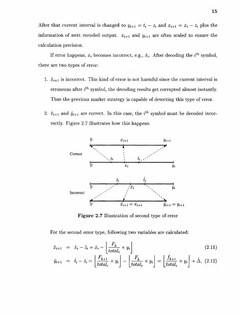
If error happens, x i becomes incorrect, e.g., x i . After decoding the ith symbol,

there are two types of error:xi+1

1. is incorrect. This kind of error is not harmful since the current interval is

erroneous after i th symbol, the decoding results get corrupted almost instantly.

Thus the previous marker strategy is capable of detecting this type of error.

2. and yi+1 are correct. In this case, the i th symbol must be decoded incor-

rectly. Figure 2.7 illustrates how this happens.

Figure 2.7 Illustration of second type of error

For the second error type, following two variables are calculated:

16

where fk+1 is the frequency of symbol k + 1 in frequency table, and A = 0 or 1. If

where A = 0 or 1. This means, if the difference caused by the error equals to

the distance difference calculated in the current interval (first condition), and the

difference between frequency of the symbol with correct value and that of the symbol

with incorrect value is not larger than 1 (second condition), the second type of error

occurs.

An example of this type of error is when the error occurs in the first encoded

byte. The adaptive encoding algorithm is applied and it assigns an initial weight of 1

to each alphabet symbol and add 1 for each occurrence. total s and y1 are initialized

to s. fk = 1, Fk = k and Fk = k for every k and k make the two conditions true.

This means the first encoded output should be extra protected.

This type of error is more harmful than the first type since the current interval

is correct, the next incorrect symbol cannot be decoded until the incorrect part of

frequency table that is caused by the error is used and the impact of this incorrectly

decoded symbol to the frequency table accumulates high enough. The decoder will

generate a long run of correct symbols between two incorrect symbols. If the first

error cannot be detected (e.g., by previous marker strategy), a long error propagation

distance will occur. Simulation result shows this kind of error occurs with probability

around 10 -5 .

To cope with this type of error and also reduce the redundancy, since the

second error type happens much less frequently than the first type, a block length is

selected such that it is much larger than the previous marker strategy's block length,

and a marker is added such that its value equals to: (sum value of all symbols in the

17

block) mod. (s). This approach is called sum marker strategy and it is used with

previous marker strategy to detect the error. The probabilities of two types of error

can be derived by integrating the possibilities for them to happen according to their

frequency in the frequency table.

2.3.2 Experiments

The previous marker strategy is used in the experiments. For a marker block length

m, the percentage of file expansion is r+-2 . Elmasry [16] indicated that using an

arbitrary value of marker may incur a large file expansion, i.e., large redundancy.

This, along with the fact that the second type of error occurs much less frequently,

necessitates that the marker block length of sum marker strategy should be chosen

large.

The adaptive coding is used, e.g., algorithm proposed by Jones [25], which

assigns an initial weight of 1 to each alphabet symbol and add 1 for each occurrence.

Let s be the size of source alphabet, n i the number of occurrences of i th symbol in

the alphabet, and l the length of source data. This implies that

length, before adding any kind of detection strategy, is

Applying the previous and sum marker strategies, the block lengths for them are m 1

and m2 (m i < m2 ), respectively, and the source data length becomes

The number of ith symbol in the alphabet becomes

the probability that sum marker is the ith symbol in the alphabet.

are the number of added marker by previous and sum marker strategy, respectively.

The code length after applying previous and sum marker strategy (i.e., combined

18

strategy) is,

gives the redundancy added by the combined scheme.

The comparison of the combined strategy and the previous marker strategy

is based on same amount of redundancy. 256 x 256 LENA is used as source file.

Simulation shows the combined strategy with m 1 = 40 and m2 = 800 has similar

redundancy to the previous marker strategy with m 1 = 35. Their PDFs of error

propagation distance are shown in Figure 2.8.

Figure 2.8 Error propagation distance PDF of combined strategy and previousmarker strategy

One can see that the combined strategy has a better PDF than previous marker

strategy. (The number with smaller propagation distances is more). Moreover,

what is not shown in the figure is that the previous marker strategy has several

samples with large propagation distance (> 200), but most of them are detected in a

small delay by the combined strategy. This means the combined strategy has better

L2 - L1L1

19

delay characteristic and in turn, less redundancy and larger throughput obtained in

communication networks.

2.4 A Comparison Between Two Error Detection Techniques UsingArithmetic Coding

2.4.1 Forbidden Symbol Approach and Marker Symbol Approach

Of the joint source and channel coding using variable length codes, Boyd et al. [13]

proposed a detecting approach which introduces redundancy by adjusting the

coding space such that some parts are never used by encoder. If decoding process

enters the forbidden region, an error must have occurred. This approach is called

forbidden symbol approach and it is widely used. Kozintsev et al. [22] analyzed the

performance of this approach in communication system by introducing "continuous"

error detection. The redundancy versus error detection time was studied. Pettijohn

et al. [21] extended this work in sequential decoding to provide error correction

capability. Another idea of using arithmetic codes for error detecting was proposed

by Elmasry [16] and extended in this chapter, where the redundancy needed for

error detection is introduced to the source data before compression in the form of

periodically inserted markers. The decoder examines the reconstructed data for the

existence of the inserted markers. An error is indicated if a marker does not appear

in its proper location.

Two approaches are referred to as forbidden symbol approach and marker

symbol approach, respectively. Next section compares the error detection capability

of these two approaches in terms of redundancy and error propagation distance (i.e.,

error detecting time in [22]), which mainly determine the performance of system

based on the approach. The comparison shows that while two approaches basically

have the same error detection capability, they should be applied to different kind of

systems [27, 28].

20

2.4.2 Comparison of Redundancy and Error Propagation Distance

For forbidden symbol approach, the redundancy and error propagation distance are

analyzed by Kozintsev et al. [22], where the forbidden symbol is assigned probability

E (0 < E < 1). A random variable Y1 with geometric distribution is modeled to

represent the number of symbols it takes to detect an error after it occurs, i.e., error

propagation distance:

and the probability that error propagates more than n symbols decreases with n th

order of (1 — c):

The redundancy is

For the marker symbol approach, the previous marker strategy is used (the

combined marker strategy described in Section 2.3 has similar or a little better delay

characteristics). With the previous marker strategy, a block of size m source symbols

is turned into a block of m + 1 symbols by repeating the 'Oh symbol at the ern + 1) th

location. Thus the amount of redundancy is

The PDF remains almost constant in each marker region in Figure 2.2. But

between these marker regions, PDF drops quickly. The probability that error is

checked within 1 markers can be statistically determined by simulation. Here an

approximation simply explains the result. Assuming one symbol contains c bits,

2c symbols are in the alphabet. Since even a single error will cause the decoding

process losing self-synchronization property and the decoded data being garbled,

21

when comparing the marker and the previous symbol, the probability that they are

the same roughly equals to the probability that two independent numbers selected

Letting random variable Y2 represent

number of markers that error propagates, the probability that error propagates more

than l markers, i.e., the misdetection probability, is,

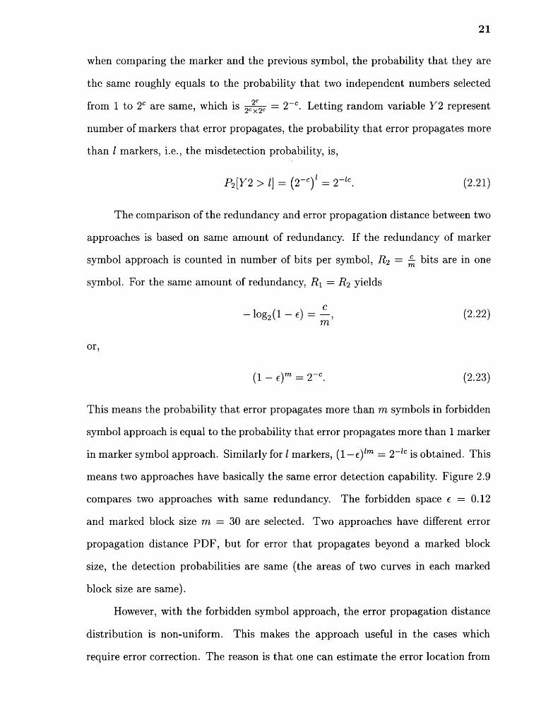
The comparison of the redundancy and error propagation distance between two

approaches is based on same amount of redundancy. If the redundancy of marker

symbol approach is counted in number of bits per symbol, R2 = c/m bits are in one

symbol. For the same amount of redundancy, R1 = R2 yields

This means the probability that error propagates more than m symbols in forbidden

symbol approach is equal to the probability that error propagates more than 1 marker

in marker symbol approach. Similarly for l markers, (1-- c)" = 2 -1c is obtained. This

means two approaches have basically the same error detection capability. Figure 2.9

compares two approaches with same redundancy. The forbidden space e = 0.12

and marked block size m = 30 are selected. Two approaches have different error

propagation distance PDF, but for error that propagates beyond a marked block

size, the detection probabilities are same (the areas of two curves in each marked

block size are same).

However, with the forbidden symbol approach, the error propagation distance

distribution is non-uniform. This makes the approach useful in the cases which

require error correction. The reason is that one can estimate the error location from

Figure 2.9 Comparison of error propagation distances of two approaches

the geometrically distributed error propagation distance. While in marker symbol

approach, the error location PDF within a marked block is approximately uniformly

distributed. One can only guess the error in terms of marked block, but does not

know the error position within the block.

Although the marker symbol approach is less efficient in error correction, it is

simple and does not change the entropy code in encoder and decoder. The approach

can be applied to existing systems without modification of encoder and decoder.

Moreover, though forbidden symbol approach provides continuous error detection,

in current packet switching networks there is no need for high frequency of error

checking. By introducing several markers in a packet, the marker symbol approach

is capable of detecting errors with less computation complexity.

2.5 Conclusion

In this chapter, a JSCC design with arithmetic codes is proposed. The self-

synchronization property of arithmetic codes is used to detect error, at the price of

introducing error propagation. The error propagation distance PDF is discussed and

23

modeled for both text and image transmission. The arithmetic coding with adaptive

algorithm is discussed and two types of error are found. The first type of error is

suitable for previous marker strategy to detect and for the second type of error, a

new detection strategy is introduced. Two strategies are combined to detect errors.

Simulation result shows that this combined scheme is capable of detecting error with

small delay, which gives more code rate and throughput in communication networks.

A comparison of the error detection capability is presented between two error

detection approaches with arithmetic coding, i.e., forbidden symbol approach and

marker symbol approach. It shows two approaches have basically the same error

detection capability. With its geometric distribution of error propagation distance,

the forbidden symbol approach is useful in the cases where the error location can be

estimated for error correction. The marker symbol approach is simple and does not

change the source encoding and decoding design. Though forbidden symbol approach

provides continuous error detection, its high frequency of error checking is generally

not needed in packet switching networks. The marker symbol approach with less

computation complexity may be a better choice in this case.

CHAPTER 3

ERROR RECOVERY PROTOCOL OF THE PROPOSED JOINTSOURCE AND CHANNEL DESIGN

With packet switching networks, error recovery techniques conventionally use

Automatic Repeat Request (ARQ) protocols, such as Cyclic Redundancy Codes

(CRC). These techniques utilize a channel coding approach that divides the data

into blocks of length k bits and adds redundancy to each block to form code words of

length n bits. The ration is referred to as the code rate [29]. The added redundancy

(n — k) is utilized by the receiver for error detection. Since compressed data is

intolerant to errors, a single unrecovered channel error results in the loss of the self-

synchronization property of the compressed data, which causes the reconstructed

data to become garbled from the point where the error occurred to the end of the

decoded sequence. For conventional ARQ protocols to achieve reliable transmission,

they either

1. use an excessive amount of redundancy, which decreases throughput efficiency,

2. increase the code word size, n, which increases the code complexity and the

transmission delay, or

3. utilize fixed-length compression techniques, which affects the obtained com-

pression gain and in turn decreases the achieved throughput efficiency.

Therefore, in this chapter, an ARQ protocol using the joint source and channel

coding design (JARQ protocol) is introduced in Section 3.1 that utilizes the self-

synchronization property of the data compression for the benefit of error recovery.

By taking the advantage of nonuniform error propagation distance PDF, packet

combining is performed in Section 3.2 to improve system performance.

24

25

3.1 Introduction to the JARQ Protocol

With the delay characteristic explained in Section 2.2, error detection may occur

because of an error in a previous packet rather than in the current one. To account

for this scenario, a modification in the conventional ARQ protocol, e.g., Go-Back-N

request for retransmission algorithm [30, 31], was developed. This modified algorithm

is called the JARQ protocol and in particular, the Go-Back-(N, M) (M > 1) protocol.

This protocol accepts a packet only after checking that no errors are detected when

decompressing it as well as the M packets that follow it [32-34].

In this analysis, M + 1 detection states (state 0 to state M) are defined and

the state number stands for the number of packets held at the receiver previous

to the current packet. The detection state flow starts from state 0, as shown in

Figure 3.1. State i (1 < i < M) is obtained through receiving i consecutive packets

with no error detection. Once an error is detected in a received packet, the detection

process returns back to state 0, which means that a retransmission is requested.

Upon reaching state M, if no error is detected in the received packet, the earliest

held packet will be released, the state will remain unchanged, and a new one will be

received. State M is obviously the desired working state.

Figure 3.1 Detection state flow of Go-Back-(N, M) (M >= 1) protocol

When an error is detected, if M is large, a large number of packets have to

be retransmitted, which decreases the throughput. On the other hand, a large M

is desirable because checking more packets (and as a result more marker locations)

reduces the probability of misdetection. As seen in Figure 2.2 and Figure 2.3, errors

26

normally will not propagate to a large number of bytes. Because a packet contains

several blocks, M = 1 or 2 can be selected in most applications. This implies small

overhead.

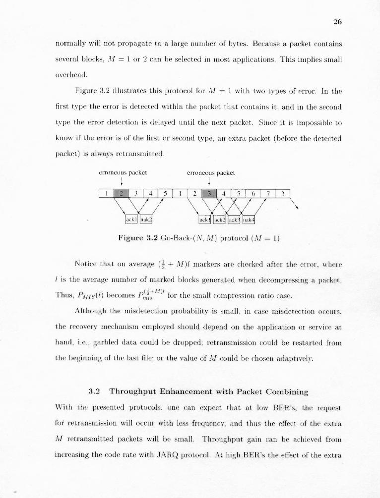
Figure 3.2 illustrates this protocol for M = 1 with two types of error. In the

first type the error is detected within the packet that contains it, and in the second

type the error detection is delayed until the next packet. Since it is impossible to

know if the error is of the first or second type, an extra packet (before the detected

packet) is always retransmitted.

Notice that on average + M)l markers are checked after the error, where

l

is the average number of marked blocks generated when decompressing a packet.

Thus, Pm s (l) becomes Pmis(1/2+M)l (1/2+M)l for the small compression ratio case.

Although the misdetection probability is small, in case misdetection occurs,

the recovery mechanism employed should depend on the application or service at

hand, i.e., garbled data could be dropped; retransmission could be restarted from

the beginning of the last file; or the value of M could be chosen adaptively.

3.2 Throughput Enhancement with Packet Combining

With the presented protocols, one can expect that at low BER's, the request

for retransmission will occur with less frequency, and thus the effect of the extra

M retransmitted packets will be small. Throughput gain can be achieved from

increasing the code rate with JARQ protocol. At high BER's the effect of the extra

27

retransmitted M packets will overcome the gain obtained from increasing the code

rate, and JARQ protocol is expected to give less throughput than conventional ARQ

protocols. Note, however, that at high BER's, JARQ can be used as the outer code

(in a concatenated coding approach), where the inner code is designed for error

correction. With this approach, a decoding failure from the inner code produces a

burst error. With concatenated codes, interleaving is often used for the outer code.

However, if JARQ is to be used as the outer code, interleaving can be avoided since

JARQ's error detection capability is not affected by the error pattern.

Also note that with JARQ, the decoder has knowledge of the PDF of the

detected error's location, as explained in Chapter 2. This can be utilized to

further improve the achieved throughput. With JARQ, instead of performing

de-interleaving, the receiver can perform packet combining [35].

Note that when using conventional ARQ protocols, the decoder estimate of

the error location PDF is a uniform distribution (since interleaving spreads the error

throughout the entire frame and the decoder cannot pinpoint the exact location of

the error in each packet). This is not the case with JARQ. With JARQ, if the

receiver receives two consecutive noninterleaved frames with error and these two

frames represent the same data: one is the original transmission, while the other

is the retransmission, a second retransmission can often be avoided. Based on the

estimation of the delay PDF in Figure 2.2 and Figure 2.3, the decoder can pinpoint

the location of the error in each frame to particular packets with high probability.

Then packet combining is performed (where packets with error are dropped from each

frame), and the resulting combined frame is decompressed error-free. This signifi-

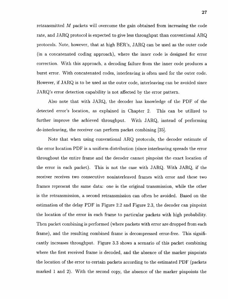
cantly increases throughput. Figure 3.3 shows a scenario of this packet combining

where the first received frame is decoded, and the absence of the marker pinpoints

the location of the error to certain packets according to the estimated PDF (packets

marked 1 and 2). With the second copy, the absence of the marker pinpoints the

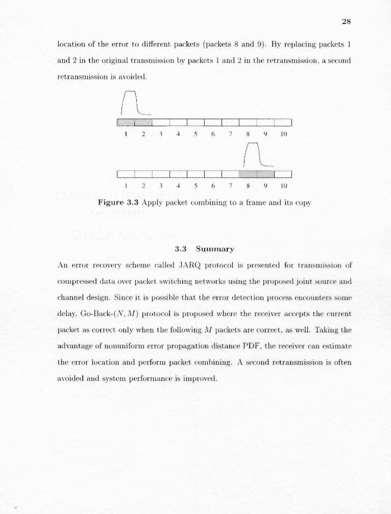
28

location of the error to different packets (packets 8 and 9). By replacing packets 1

and 2 in the original transmission by packets 1 and 2 in the retransmission, a second

retransmission is avoided.

3.3 Summary

An error recovery scheme called JARQ protocol is presented for transmission of

compressed data over packet switching networks using the proposed joint source and

channel design. Since it is possible that the error detection process encounters some

delay, Go-Back-(N, M) protocol is proposed where the receiver accepts the current

packet as correct only when the following M packets are correct, as well. Taking the

advantage of nonuniform error propagation distance PDF, the receiver can estimate

the error location and perform packet combining. A second retransmission is often

avoided and system performance is improved.

CHAPTER 4

THROUGHPUT ANALYSIS OF JARQ PROTOCOL ONINDEPENDENT CHANNEL

The previous chapter has introduced a joint source and channel design using

arithmetic. Because of the self-synchronization property, a delayed detection error

recovery approach, JARQ protocol, is presented. In this chapter, the performance

of JARQ protocol on independent channel is analyzed. Section 4.1 introduces signal

flow graph to find the average transmission time and hence the throughput. Although

the analysis shows the performance is degraded because of extra retransmissions,

it can be improved by the large code rate discussed in Chapter 3, or the optimal

case in Section 4.2, or the packet combining in Section 4.3. Simulation results in

Section 4.4 show the performance and validate the analysis.

4.1 Throughput Analysis of Go-Back-(N, M) Protocol

The signal flow graph is used to derive the performance of JARQ protocol. A signal

flow graph [36, 37] is a diagram which represents a set of simultaneous equations. It

consists of a graph in which nodes are connected by directed branches. The nodes

represent each of the system variables. A branch connected between two nodes

acts as a one-way signal multiplier: the direction of signal flow is indicated by an

arrow placed on the branch, and the multiplication factor (transmittance or transfer

function) is indicated by a letter placed near the arrow.

To make a comparison, the signal flow graph of conventional Go-Back-N

protocol is first shown in Figure 4.1. In the figure, R(i) is used to represent the

situation that the ith packet has just been transmitted or retransmitted while D(i)

the situation that ACK/NAK is expected in the sender. p is the probability that

error is occurred in a packet, i.e., packet error rate. It is assumed that any error

would be detected. q = 1 — p is the probability that packet is transmitted error-free.

29

30

Figure 4.1 Signal flow graph of Go-Back-N protocol

z is the time to transmit one packet and assuming that in one round-trip delay, s

packets are transmitted. This is denoted as z^s in the signal flow graph.

Note that the reverse channel, i.e., the channel sending acknowledgment back,

is considered error-free because of following two reasons. 1) ACK/NAKs are usually

small so the probability that they are corrupted is hence small; 2) Cumulative

acknowledgment allows an ACK acknowledge all packets already received [38].

The signal flow graph of Go-Back-(N, M) protocol is shown in Figure 4.2.

Note that once error is detected in packet i, retransmission begins from packet i M

Figure 4.2 Signal flow graph of Go-Back-(N, M) protocol

at node R(i — M) for Go-Back-(N, M), while retransmission begins just from packet

i at node R(i) for Go-Back-N in Figure 4.1. For any packet, e.g., packet i, in

addition to node D(i), there are another M nodes, 2 1 , 22 , • • • , M. Signal flow arrives

31

when error is detected at D(i + M + 1 — j) and retransmission

begins from packet i + 1— j. For example, if M = 3 and error is detected in packet 7,

retransmission will begin from packet 4 and go through the node 4 1 , 52 , 63 and finally

reach D(7) to be checked again. Note that these M nodes, i i to iM , are different

from each other because packet i is retransmitted when error is found in any of the

packet with number from i to i + M. Node D(i) and iM to i 1 represent the packet i

when error occurs in packet i and packet i + 1 to i + M, respectively.

Since all the retransmission flows are similar, one flow is analyzed, e.g., packets

are retransmitted and checked at (i — M) 1 , (i — M + 1) 2 to D(i). Let H(z) be the

transfer function of transmitting two continuous packets, e.g., packet i —1 and packet

i. Repeatedly applying the serial and parallel merge to simplify the signal flow graph

in Figure 4.2 gives

Therefore, the throughput of the Go-Back-(N, M) protocol ηgbnm is obtained through

Note that the first M and last M packets are not considered in above derivation,

whose signal flow graphs are different from above. But same result can be obtained

32

when L goes to infinity. One can see ηgbnm changes with q to the order of M + 1.

If q is big, e.g., q P.-; 1, the impact of retransmission of M more packets is small. If

q is small, ηgbnm drops quickly. Luckily, M is small in most applications. Note that

which is the throughput of conventional

Go-Back-N protocol [39].

4.2 Optimal Case for Go-Back-(N, M) Protocol

Go-Back-(N, M) protocol always retransmits M more packets to correct possibly

long-propagated errors. Eq.(4.4) shows that its throughput changes with q M+ 1 .

When q is small, even a small M makes the throughput drop quickly. This can

be improved if the location of error is known and only the packet that contains the

error is retransmitted.

For a packet with length L and an error propagation distribution with PDF

f (x) and CDF F(x), the probability that an error found in the packet does exist in

the packet is

Then the probability that an error found in the packet but actually exist in previous

packet, i.e., error propagates through 1 packet, is Ψ(F, 2L) — Ψ(F, L), and more

generally, the probability that the error propagates through i packets, 0 <= i <= M,is

If retransmission starts from packet i, the corresponding

-1-p,+i

sthroughput is / and overall throughput for this optimal case is1

However, in practice the location of error is unknown and Ψ(F, L) generally

cannot determine the retransmission position. For a good error propagation distance

PDF, such as in the text transmission, the error location can be determined with

33

a high probability. To do this, a propagation distance lfun is calculated such that

F (lfull) almost approaches 1. For a packet with length L > l full , if error is found at

the position after l full bits, the error is located in this packet with a high confidence

and retransmission just starts from it. If error is found within l full bits, previous

packet is retransmitted. The throughput for this case (not as good as the optimal

case but much more practical) is

where the probability that the error traverses more than 1 packet is ignored because

F (lfull) 1. Generally, the smaller l full , the better performance obtained.

4.3 Throughput of Go-Back-(N, M) Protocol with Packet Combining

As explained in Section 3.2, packet combining can be performed on the retransmitted

packets since the delay PDF is not uniformly distributed. Two cases are considered.

In first case, packet combining is performed only on the packet that is being detected

and retransmitted, i.e., only 1 packet is buffered. In second case, all the N packets

after the packet in first case are buffered and packet combining is performed on all

these packets, just as shown in Figure 3.3.

For the first case, to simplify the derivation, it assumes that by using packet

combining, the overall packet error rate is reduced by the ratio of a, where 0 < a < 1.

Denoting the new packet error rate as P = ap, the probability that packet is correct

The signal flow graph of Go-Back-(N, M) protocol with packet combining is

shown in Figure 4.3. To simplify, only the node from i — M to i + 1 are shown.

Note that for each packet i, another node, D'(i), is added, which is different

from D(i) because packet combining is performed at D'(i), while there is no retrans-

34

Figure 4.3 Signal flow graph of Go-Back-(N, M) protocol with packet combining

mitted packet at node D(i). Packet combining is performed at node (i — M) 1 ,

The transfer function for transmitting L packets can be obtained as

For given p, s, and M, ηcomb changes with a and their relation is shown in

Figure 4.4. Figure 4.4 shows that η comb increases rapidly when a is big is small),

e.g., a < 1. When a is large, (around 5 in Figure 4.4), ηco mb almost approaches its

35

Figure 4.4 Relation between ηcomb and a, for given p, s and M.

maximum value. This means one can simply apply the maximum throughput that

the packet combining can achieve. ηcomb will obtain its maximum value when agoes

to infinity, which is

To see how much throughput gain can packet combining obtain, the gain is

calculated,

Figure 4.5 shows the value of G with respective to p, 0 < p < 1. There are two

points with G = 1. When p = 0, both scheme obtain 100% of the throughput. When

This means the detriment of retransmitting M more packets is

bigger than the merit of packet combining, and at

packet combining outperforms the

redundancy of retransmitting M more packets and G > 1 is obtained.

36

Figure 4.5 Packet combining gain

For the second case, N more packets are buffered. Since packet combining is

performed to all these packets, the packet error rate is reduced by approximately α/N.

The result in Eq.(4.10) is used and it gives

The throughput is bigger than that in the first case, and it increases with N, which

is shown in the simulation.

4.4 Simulation Results

4.4.1 Selection of Code Rate for JARQ and Conventional ARQ

For the conventional ARQ schemes, the selected code rate, n, must be small enough

so that the probability of catastrophic error (undetected error pattern) is very low.

Although with JARQ protocol, a channel error will be detected eventually, to draw

a fair comparison, PE PMTS, the probability of undetected error in JARQ, is equated

to the probability of catastrophic error in conventional ARQ systems. The difference

between the two scenarios should be emphasized. With conventional ARQ protocols,

37

when the channel decoder supplies an incorrect codeword to the source decoder, there

is no way to recover from this error. While with JARQ, a missed error will always

propagate and garble the remaining data and eventually, it will be detected.

Since the compression ratio

In the simulation performed here, ATM cells is

used as the transmitted packet, where the packet size is 53 bytes [40]. For a marked

block size of m = 30 and R = 1.47, the number of marked blocks in an ATM cell

The code rate is chosen to bound the misdetection probability by 10',.._

i.e.,

This gives M = 2 for the above parameters.

For image data, since the above approximation cannot be used, simulation is

relied on to find an m that bounds us to the same bound of misdetection probability.

If applying Go-Back-(N, M) with M = 2, the value of m is found to be around 20

from simulation. Thus the code rates are N and V for text and image transmission

respectively.

The code rate of conventional Go-Back-N protocols, , is about to determined

to give a probability of catastrophic error in the same vicinity for the same packet

size. Eq.(4.15), from [29], can provide a bound for this probability using linear block

codes (e.g., CRC),

one can solve for k and obtain the values of the code rate, , with ARQ. A codeword

length n equal to the packet length as the entire ATM cell is used i.e., n = L = 53 x 8

bits. This gives n — k ; -- .--i, 37 bits and 17,-ci r-:.1 0.9127 for conventional ARQ.

38

4.4.2 Throughput Comparison

Simulation is carried out using adaptive arithmetic coding [25]. Plain English text

and the 256 x 256 LENA in the DCT domain are used.

Figure 4.6 shows the simulation results obtained for throughput versus BER,

using N = 4 and M = 2. Figure 4.7 repeats the same simulation for the case of

N = 64 and M = 2. The figures show that JARQ obtains a larger throughput

than ARQ at low BER's because of its higher code rate, for either text or image

transmission. Notice that as the BER increases, the performance of JARQ degrades

more than with conventional ARQ (crosses over in the figure). This is because at

a high BER, the detriment of the extra packet transmission is more than the gain

obtained from increasing the code rate.

Figure 4.6 Throughput comparison of Go-Back-(N, M) and Go-Back-N protocols(N = 4 and M = 2)

Figure 4.8 and Figure 4.9 show the performance of Go-Back-(N, M) with packet

combining for N = 4, M = 2, and N = 64, M = 2, respectively. Text transmission

is used in these figures (similar results are obtained for image transmission). Overall,

JARQ with packet combining improves throughput performance, especially at high

Figure 4.7 Throughput comparison of Go-Back-(N, M) and Go-Back-N protocols(N = 64 and M = 2)

BER's. Notice that packet combining gives more throughput gain for a large window

size than for a small one. This should be expected since two copies of a long frame

with errors are more likely to contain non-overlapping error.

4.5 Summary

In this chapter, the throughput of JARQ protocol is analyzed for independent channel

by using signal flow graph. Suffered from the delayed detection, the throughput

changes to the order of number of extra retransmissions. However, this impact is

alleviated when BER is small. At high BER's, packet combining is introduced and

significant throughput gain is achieved. In addition, The throughput is increased

with a larger code rate, compared with conventional ARQ scheme. The simulation

results validate the analysis.

Figure 4.8 Throughput of Go-Back- (N, M) protocol using packet combining (N = 4and M = 2)

40

Figure 4.9 Throughput of Go-Back-(N, M) protocol using packet combining (N =64 and M = 2)

CHAPTER 5

THROUGHPUT ANALYSIS OF JARQ PROTOCOL ONNONINDEPENDENT CHANNEL

Chapter 3 proposes a JARQ protocol for the joint lossless-source and channel coding

scheme introduced in Chapter 2. The throughput of this protocol on independent

channel is analyzed in Chapter 4. In this chapter, its throughput on nonindependent

channel is analyzed.

5.1 Introduction

Unlike the independent channel which is modeled by bit error rate (BER), a

non-independent channel is often modeled by Markov process. Gilbert [41] first studied

the Markovian type of channel errors with two-state model. Later Fritchman [42]

proposed finite-order model which can be represented by a finite-order Markov

process. The k th-order Markovian channel model applies a k-dimensional transition

matrix to represent the relation between the correctness of a received packet and

the error conditions of its k preceding packets. A gap error model was also proposed

to simulate nonindependent channel by Kanal and Sastry [43] which models the

number of correct (erroneous) packets between two consecutive erroneous (correct)

packets as random variables.

Although the second or higher-order Markov process provides a more accurate

model of nonindependent channel condition, recent studies by Wang and Chang [44],

Abdi [45], and Zorzi et al. [46] show that a first-order Markovian channel which

uses only the information of immediately preceding packet is adequate to model the

nonindependent channel. The amount of uncertainty in the current packet provided

by the packets preceding the previous one is negligible.

In the rest of this chapter, Section 5.2 describes the first-order Markovian

channel model. The throughput of Go-Back-(N, M) protocol under nonindependent

41

42

channel is analyzed in Section 5.3. The performance of JARQ protocol without

packet combining and JARQ protocol with packet combining are simulated in

Section 5.4.1 and Section 5.4.2, respectively. Final section draws some conclusions.

5.2 Nonindependent Channel Model

The two-state models by Gilbert [41] and Elliot [47] are examples of first-order

Markov process. It consists of two states which are called G (for good) and B (for

bad or for burst). Similar ON-OFF model is also widely used, where an ON (active)

state and an OFF (silent) state are introduced [48-50]. Transitions are made between

two states according to transition probabilities. Burst errors are generated bit by bit

each time the B (or ON) state has arrived. A Similar threshold model is proposed by

Zorzi et al. [51] who extended the model to generate error frame by frame, or packet

by packet.

The nonindependent channel model used in this chapter is based on the

threshold model in [51] and summarized in [52]. It is shown that a sequence of

packet is correct or erroneous can be approximated by means of a simple two-state

Markov chain whose transition probability matrix is given by

where q and 1 — p are the probabilities that the j th packet is correct, given that

packet was correct or incorrect, respectively. p and 1 — q are the

probabilities that the j th packet is incorrect, given that the (j — 1) th packet was

incorrect or correct, respectively. Note that TIT represents the average length of a

burst of packet errors. The channel condition of forward channel (i.e., sender sends

packet to receiver) is focused and the transition matrix of backward channel (i.e.,

receiver responds acknowledgment to sender), MB, is considered error-free. (See

Section 4.1.) The error pattern relation between two packets being x packets apart

43

The steady state can be obtained when (MF)x approaches a matrix A with x ---÷ oo.

Each row of A is the same probability vector a = [πc π e], where 71-c and Ire are

the steady state probability of a correct transmission or an incorrect transmission,

respectively [53]. Also from [53], the steady state probability is,

For a fading multipath channel with a fading margin F, the average frame error

rate (FER), i.e., packet error rate, can be found in [541 as

From [51], p is given by

In the above, Jo () is the Bessel function of the first kind and zeroth order. fdT is

the normalized Doppler bandwidth which describes the correlativity or burstness in

the nonindependent channel. Q(., .) is the Marcum Q function, given by

where J is the modified Bessel function of the first kind and zeroth order. Given F

and fdT, the Markov parameter p and q are obtained from Eq.(5.4) to Eq.(5.7).

44

5.3 Signal Flow Graph of Go-Back-(N, M) Protocol and ThroughputAnalysis

The performance of ARQ protocol on nonindependent channel has been widely

studied [55-58]. Cho and Un [55] investigated the effect of forward/backward channel

memory on two modified Go-Back-N protocols. Lu and Chang [56] used kth-order

Markovian channel model and gap error model [43]. The performance of Go-Back-N

protocol with unreliable feedback and the comparison of Go-Back-N and selective

repeat protocols on nonindependent channel were analyzed by Zorzi and Rao [57] and

Chuang [58], respectively. In this study, the first-order Markovian channel model is

used and performance of the delayed detection, i.e., M more retransmitted packets,

is investigated [59-61].

If transmitting L packets, the signal flow graph of the Go-Back-(N, M) protocol

under nonindependent channel is shown in Figure 5.1. Similar notations to that

Figure 5.1 Signal flow graph of Go-Back-(N, M) protocol on nonindependentchannel

in [55] are used. Node I and node 0 denote input and output nodes, respectively.

Any path leading from I to 0 corresponds to a successful transmission of these L

packets. z is the time to transmit one packet and assuming that in one round-trip

delay, s packet are transmitted. This is denoted as z' in signal flow graph. Node

Zo (i) and node Z1 (i), 1 <= i < L, denote the ith packet is transmitted correctly or

incorrectly, respectively.

45

Starting from node I, packet is either transmitted correctly with probability

7, to node Z0 (1), or transmitted incorrectly with probability 'Fe to node Z1 (1). At

node Z 1 (1), retransmission is requested. After time t = s + 1, i.e., round-trip delay

plus the time to transmit one packet, the retransmitted packet is either incorrectly

received with probability p(t), the probability that current packet is erroneous if the

(s + 1) th preceding packet is erroneous, or correctly received with probability 1 — p(t),

the probability that current packet is correct if the (s + 1) th preceding packet is

erroneous. Since M more packets have to be retransmitted and if the first one is

retransmitted correctly, the next packet is either incorrectly received and status is

back to Z 1 (1) with probability 1— q, the probability that current packet is erroneous

if the immediately preceding packet is correct, or correctly received with probability

q, the probability that current packet is correct if the immediately preceding packet

is correct, as well.

After M consecutively successful retransmission, one packet is released and

detection process arrives at node Z0 (1). At Z0 (1), packet is either transmitted

correctly with probability q to node Z0 (2), or transmitted incorrectly with proba-

bility 1 — q to node Z1 (2), since the previous packet is correctly received. After that,

signal flow repeats as the above.

Let H (z) be the transfer function of transmitting these L packets. Note that the

signal flow graph consists of two similar flows with minor difference. The transition

starting from node I has probability πc and πe, while the transition starting from

node Zo (i), 1 < i < L, has probability q and 1 — q. The transfer function from node I

to node Z0 (1) is obtained first by applying the serial and parallel merge in signal flow

graph. Let t = s + 1, round-trip time plus the time to transmit a packet, which is the

time from the start of transmission of a packet to the receipt of its acknowledgment,

46

the transfer function is

Finally the transfer function of transmitting L packets is obtained as

represents the average time taking to traverse L packets in the

signal flow graph [37], the throughput can be obtained by limiting L to infinity as

Therefore, the throughput when L = 1 is

and the throughput when L approaches infinity,

5.4 Simulation Results

5.4.1 Simulation Results without Packet Combining

In the simulation, the threshold model previously described is used. Choosing

different values of fading margin (F) and normalized Doppler bandwidth (fdT),

47

different Markov parameter p and q are calculated and used in the simulation. With

fdT = 0.01, the channel is very correlated (long bursts of packet errors). With

fdT = 1.0, the channel becomes almost independent (short bursts of packet errors).

The average packet error rate PE is calculated by Eq.(5.4) and to make a comparison,

the corresponding independent channel model is also considered with the same packet

error rate. The round-trip delay is s = 9, i.e., t = 10. Go-Back-(N, M) protocol is

used with M 2.

Figure 5.2 shows the theoretical throughput calculated by Eq.(5.13) and the

simulation results. fdT = 0.03 and fading margin ranging from F = 4.0 dB to

F = 20.0 dB are used. The throughput increases with fading margin. The figure

shows the simulation results validate the analysis.

Figure 5.2 Comparison of theoretical throughput and simulation result of Go-Back-(N, M) protocol on nonindependent channel ( fdT = 0.03)

Figure 5.3 compares the throughput with different normalized Doppler band-

width. F = 5.0 dB and F = 15.0 dB are used. The throughput of independent

channel corresponding to the nonindependent channel with same PE is also plotted

to show the comparison. It is clear that the throughput increases (decreases)

48

when the channel becomes more correlated (independent). This means the trans-

mission benefits from channel correlation. At around fdT >= 0.3, the channel

can be considered almost independent as the throughput approaches that on the

independent channel.

Figure 5.3 Throughput comparison of Go-Back-(N, M) protocol on nonindependentchannel and independent channels (F = 5.0 dB and F = 15.0 dB)

5.4.2 Simulation Results with Packet Combining

Figure 5.4 to Figure 5.9 show the throughput of Go-Back- (N, M) on nonindependent

channel with packet combining. The round-trip delay s is used as combining window

size because it implies the number of packets which have performed packet combining

in a round-trip delay time.

Figure 5.4 to Figure 5.7 compare the throughput with and without packet

combining at different window size. The normalized Doppler bandwidths are fdT =

0.01, 0.03, and 1.0 to represent different channel correlativity. One can see packet

combining improves performance, especially at small F (large error rate) and large

combining window size. At a large window size, e.g., s = 64 in Figure 5.7, the

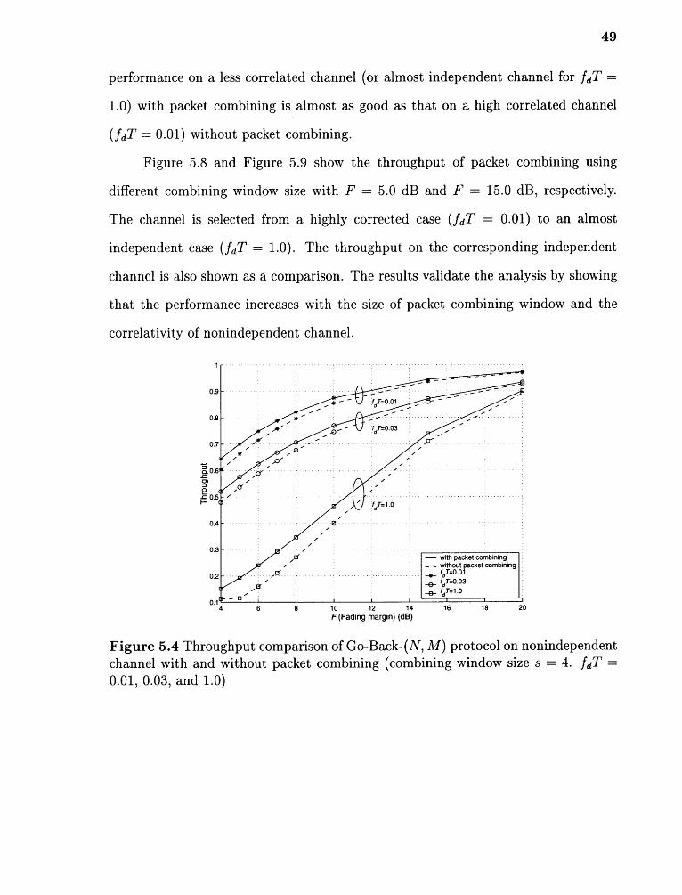
49

performance on a less correlated channel (or almost independent channel for fdT =

1.0) with packet combining is almost as good as that on a high correlated channel

without packet combining.

Figure 5.8 and Figure 5.9 show the throughput of packet combining using

different combining window size with F = 5.0 dB and F = 15.0 dB, respectively.

The channel is selected from a highly corrected case (fdT = 0.01) to an almost

independent case (fdT = 1.0). The throughput on the corresponding independent

channel is also shown as a comparison. The results validate the analysis by showing

that the performance increases with the size of packet combining window and the

correlativity of nonindependent channel.

Figure 5.4 Throughput comparison of Go-Back-(N, M) protocol on nonindependentchannel with and without packet combining (combining window size s = 4. fdT =0.01, 0.03, and 1.0)

50



51


Figure 5.8 Throughput comparison of Go-Back-(N, M) protocol on nonindependentchannel with and without packet combining (combining window size s = 4, 10, 20,and 64. F = 5.0 dB)

52

Figure 5.9 Throughput comparison of Go-Back-(N, M) protocol on nonindependentchannel with and without packet combining (combining window size s = 4, 10, 20,and 64. F = 15.0 dB)

5.5 Conclusion

This chapter presents the performance of an ARQ protocol based on joint source

and channel coding scheme on nonindependent channel. Simulation result shows

it matches the theoretical throughput derived by signal flow graph. A good

performance can be obtained at high correlation (at small fdT). The throughput

decreases when the channel becomes less correlated, i.e., more independent (at large

fdT), and approaches the throughput on the independent channel.

CHAPTER 6

JARQ APPLICATION TO WIRELESS TCP NETWORKS

One of an important application of joint source and channel coding is wireless

communication where the limited channel source (bandwidth) requires an efficient

system. This chapter applies JARQ protocol to wireless TCP networks to improve

the performance of TCP on lossy wireless link. Several wireless TCP approaches

are reviewed in Section 6.1. In Section 6.2, JARQ is introduced to the data link

layer of wireless TCP networks as a radio link layer protocol. Section 6.3 compare

the performance of TCP/ARQ and TCP/JARQ protocols and the simulation results

show a significant performance improvement by error correction in data link layer

with JARQ protocol.

6.1 Introduction

Due to the increasing need to share information between mobile users and to connect

them to the Internet, wireless is becoming a popular way to connect mobile computers

to provide applications like e-mail, web browsing, Telnet, mobile computing, etc.

An efficient data transmission protocol should be applied to provide data exchange

between mobile users in wireless networks and hosts in the existing Internet.

For the Internet, the most widely used transport layer protocol is Transmission

Control Protocol (TCP) [62-64]. TCP provides a connection-oriented, reliable,

end-to-end byte stream service by receiver's responding acknowledgment to transmitter,

providing sliding window flow control, maintaining header and data checksum, and

resequencing our-of-order data [62]. There are numerous rules regarding the initiation

and termination of a TCP connection. Figure 6.1 shows the TCP connection by

summarizing these rules in a state transition diagram.

53

54

Figure 6.1 TCP state transition diagram. Reprinted from TCP/IP Illustrated,Volume 1: The Protocols by W. Richard Stevens. Copyright © 1994 by Addison-Wesley Publishing Company, Inc.

55

To provide an easy interaction between mobile users in wireless networks and

hosts in the Internet, TCP should be applied to wireless networks to control data

transmission, as well. However, TCP is designed to perform well in traditional

wireless networks where the error rate is low and packet losses are mainly due to

the congestion in the network. TCP responds to all packet losses by shrinking

the congestion window size (cwnd) before retransmitting packets, and invoking

congestion control and avoidance algorithm [65] or fast retransmit and fast recovery

algorithm [66-68].

Although these algorithms work well to resolve congestion problems occurred

in wireline networks, unfortunately they may fail in wireless networks. On lossy

wireless link, the main reason for packet loss is the high error rate, not the congestion.

Simply applying the congestion control and avoidance algorithm to wireless networks

may result in an unnecessary reduction in the congestion window, hence in reduced

throughput and degraded performance.

Recently, several approaches have been made to alleviate this problem and make

the flow control scheme of TCP work efficiently in lossy wireless links. Balakrishnan

et al. [69], Racherla et al. [70], and Wang and Tripathi [71] summarized and compared

these approaches. The proposed TCP schemes for wireless networks can be classified

in the following categories:

1. TCP/IP header compression. The 20-byte TCP header and 20-byte IP version

4 (IPv4) header can cause a significant amount of overhead in the application

like Telnet, where a TCP segment may contain only 1 byte of data. With the

combined 60-byte TCP/IP header in the new IP version 6 (IPv6), this overhead

is more significant. It is observed that a large part of header does not change

very much in a stream of packets, so the TCP/IP header can be compressed

in such a way that the sender transmits a full header for the first time and

transmits only the small changes for the successive packets. Jacobson [72]

56

proposed TCP/IP header compression for low-speed serial links and Degermark

et al. [73] proposed the compression scheme on wireless networks. The recovery

mechanism for original full header in case of error is also discussed.

2. Split-connection protocol. This protocol splits a TCP connection into two

separate connections: one TCP connection between the sender and base station

and the other between base station and receiver. One connection is on wireless

link and the other is on wireline link for many mobile applications where the

mobile user accesses hosts in the Internet. By splitting the TCP connection,

the data flow over wireless link and data flow over wireline link are isolated

from each other and the original TCP sender is shielded from the lossy wireless

link.

Indirect-TCP (I-TCP) [74] and mobile-TCP [75] are examples of this kind of

protocol.

3. Snoop protocol. The snoop protocol introduces a "snoop agent" at base station

which monitors the packets sent to and the acknowledgments sent back by the

mobile user. A cache is maintained to buffer the unacknowledged packets and if

a packet has been lost or corrupted, it will be retransmitted by the base station

if the packet has been backed up in the buffer. The duplicated acknowledgments

are suppressed and the sender is shielded from the packet loss. Balakrishnan

et al. [76] proposed this kind of protocol.

4. Link layer solution. The idea is to add the error correction mechanism to lower

layer, i.e., data link layer, and try to correct most of errors at this layer. The

error that cannot be corrected by the limited attempts in data link layer will

be finally forwarded to TCP layer. TCP layer will see the packet with much

less error and congestion control and avoidance algorithm can work efficiently.

There are lots of work in this area [52, 77-80].

57

The advantage of this approach is that TCP layer does not need modification

and it works as usual since most of errors are corrected in lower layer and

TCP layer is shielded from the error. A natural layered architecture is also

maintained by this protocol.

5. Other methods includes explicit loss notification (ELN) [69] which explicitly

tells the mobile users that whether the packet loss is due to congestion or

channel error. Selective acknowledgment (SACK) [81] is also proposed which

provides more information than the traditional cumulative acknowledgment to

help suppress duplicate retransmissions and recover error.

Among the protocols introduced above, link layer solution is of interest because

its protocol architecture allows us to introduce ARQ protocol in data link layer

without modifying upper layers. A radio link protocol (RLP) is generally introduced

and a TCP/RLP protocol stack is developed to reduce the error rate seen by the

TCP layer and hence improve system performance. In particular, JARQ protocol is

applied and the interaction between the data link layer with JARQ and TCP layer

is analyzed to optimize the performance of TCP/JARQ protocol stack. The idea

is natural because it shows in Chapter 1 that joint source and channel design may

play an important role in wireless communication and the Internet to obtain good

performance while meeting a satisfactory QoS.

6.2 TCP/RLP Protocol Stack

Due to the high link loss rate in wireless networks, to improve communication relia-

bility and obtain good system performance, Section 6.1 shows that lower layer should

provide a number of error control methods. A practical example is code division

multiple access (CDMA) cellular system. In physical layer, forward error control

(FEC) is implemented and specified in IS-95 [82]. In data link layer, RLP performing

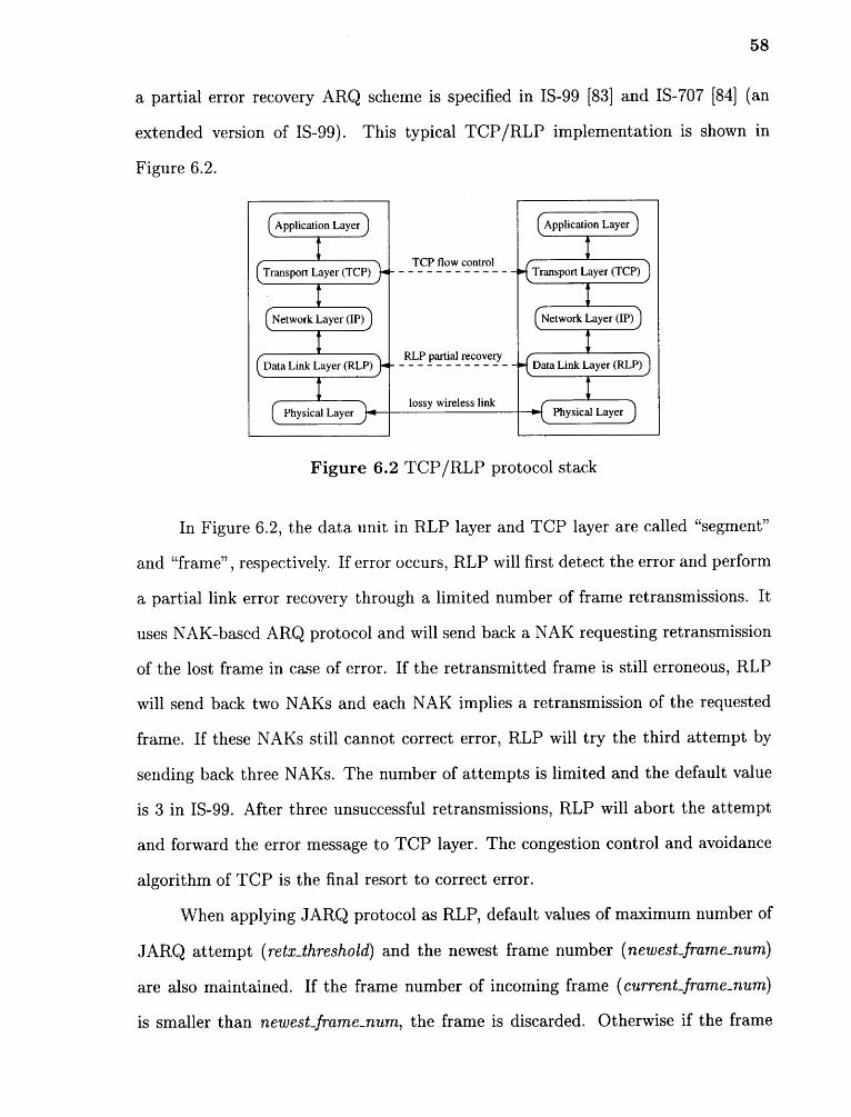
58

a partial error recovery ARQ scheme is specified in IS-99 [83] and IS-707 [84] (an

extended version of IS-99). This typical TCP/RLP implementation is shown in

Figure 6.2.

Figure 6.2 TCP/RLP protocol stack

In Figure 6.2, the data unit in RLP layer and TCP layer are called "segment"

and "frame" , respectively. If error occurs, RLP will first detect the error and perform

a partial link error recovery through a limited number of frame retransmissions. It

uses NAK-based ARQ protocol and will send back a NAK requesting retransmission

of the lost frame in case of error. If the retransmitted frame is still erroneous, RLP

will send back two NAKs and each NAK implies a retransmission of the requested

frame. If these NAKs still cannot correct error, RLP will try the third attempt by

sending back three NAKs. The number of attempts is limited and the default value

is 3 in IS-99. After three unsuccessful retransmissions, RLP will abort the attempt

and forward the error message to TCP layer. The congestion control and avoidance

algorithm of TCP is the final resort to correct error.

When applying JARQ protocol as RLP, default values of maximum number of

JARQ attempt (retx_threshold) and the newest frame number (newest_frame_num)

are also maintained. If the frame number of incoming frame (current_frame_num)

is smaller than newest_frame_num, the frame is discarded. Otherwise if the frame

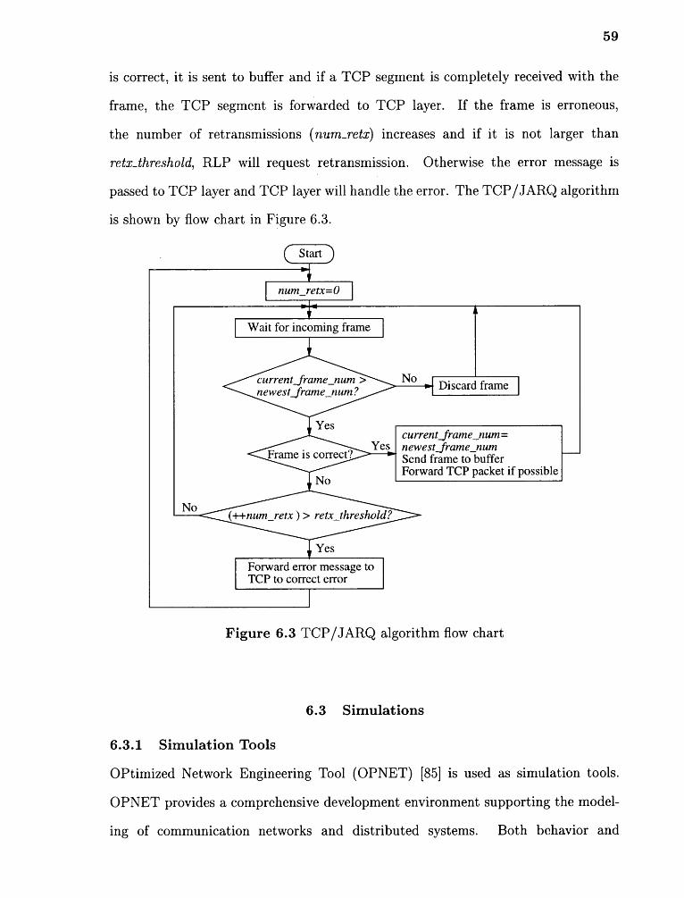
59

is correct, it is sent to buffer and if a TCP segment is completely received with the

frame, the TCP segment is forwarded to TCP layer. If the frame is erroneous,

the number of retransmissions (num_retx) increases and if it is not larger than

retx_threshold, RLP will request retransmission. Otherwise the error message is

passed to TCP layer and TCP layer will handle the error. The TCP/JARQ algorithm

is shown by flow chart in Figure 6.3.

Figure 6.3 TCP/JARQ algorithm flow chart

6.3 Simulations

6.3.1 Simulation Tools

OPtimized Network Engineering Tool (OPNET) [85] is used as simulation tools.

OPNET provides a comprehensive development environment supporting the model-

ing of communication networks and distributed systems. Both behavior and

60

performance of modeled systems can be analyzed by performing discrete event

simulations. The simulation model is shown in Figure 6.4.

Figure 6.4 OPNET network model of TCP/RLP simulation

The model consists of two nodes representing client and server, respectively.

JARQ protocol is implemented in the data link layer of client and server. An FTP

session is opened by client to retrieve files from server. Server sends back data

and a node representing lossy wireless channel is placed on the link from server to

client. The Markovian threshold model [51] described in Chapter 5 is used as burst

channel model. Traffic is monitored on the server side. The link from client to server

is considered error-free because the traffic on the link is the acknowledgment sent

from the client back to server. The acknowledgment packet is often small and since

TCP uses cumulative acknowledgment, the link can be considered error-free. (See

Section 4.1.)

Following parameters are selected in the simulation. Default TCP setting in

OPNET is used with auto-assigned maximum transmission unit (MTU). Fast retrans-

mission and fast recovery algorithm are enabled. Go-Back-(N, M) protocol with

M = 2 is applied to RLP. The average number of data link layer frame contained in

a TCP segment is 3. The retransmission threshold (i.e., maximum number of RLP

attempts before error message is forwarded to TCP layer) uses following number:

0 (namely, RLP is not used), 1, 2, 5, and 10. For the nonindependent channel

61

model, normalized Doppler bandwidth is selected from 0.01, 0.03, 0.1, and 1.0 to

represent different channel correlativity. Fading margin (F) is selected with corre-

sponding average frame error rate ranging from 0 to 0.35. Other parameters of TCP

protocol and channel model are not specified because the uniformed TCP throughput

is analyzed and the system performance without using RLP is compared with that

using RLP with different retransmission threshold.

6.3.2 Performance of TCP/JARQ Protocol Stack

Figure 6.5 to Figure 6.9 show the simulation results. TCP throughput versus different

average frame error rate in system without using RLP is shown in Figure 6.5. TCP

throughput increases as average frame error rate decreases. The most correlated

channel (fdT = 0.01) has the best performance and as the correlativity decreases,

the performance approaches that on independent channel. This is the same result

that is obtained in Chapter 5.

The advantages of using RLP with different retransmission threshold are shown

in Figure 6.6 to Figure 6.8 with fdT = 0.01, 0.1, and 1.0, respectively. The retrans-

mission thresholds are 1, 2, 5, and 10. One can see RLP improves system performance

significantly, and the larger retransmission threshold, the better performance. This

means the persistence at RLP layer is beneficial to the system. Even with one

retransmission attempt, the throughput can be almost doubled in most situations.

However, as the attempt increases, e.g., from 5 to 10 in the figure, the throughput

gain becomes less. Also as the correlativity decrease, the results approach that on

independent channel. See Figure 6.8 and Figure 6.9.

Figure 6.10 and Figure 6.11 compare the TCP congestion control window size

(cwnd) in system using RLP with one retransmission attempt and with 10 retrans-

mission attempts to cwnd in system without using RLP, respectively. The results are

obtained from above simulations and data are shown in a period of simulation time.

62

Figure 6.6 TCP throughput of system with RLP in data link layer (most correlatedchannel with fdT = 0.01)

63

Figure 6.7 TCP throughput of system with RLP in data link layer (correlatedchannel with fdT = 0.1)

Figure 6.8 TCP throughput of system with RLP in data link layer (less correlatedchannel with fdT = 1.0). The results approach that on independent channel.

Figure 6.9 TCP throughput of system with RLP in data link layer (independentchannel)

One can see the cwnd in system without RLP shrinks frequently with each error

detected. For system with RLP, as more errors corrected by RLP and less errors

seen by TCP layer, the cwnd shrinks less frequently. This means higher throughput

is achieved.

6.3.3 Performance Comparison of TCP/ARQ and TCP/JARQ Protocols

Among the introduced wireless TCP approaches, the TCP/IP header compression

scheme and SACK scheme are approaches supplementing the TCP protocol. They

can be integrated with other wireless TCP approaches, like the split-connection

protocol, snoop protocol, ELN, and link layer protocol. This section compares

these approaches by summarizing the simulation results in [69] and presenting the

performance of the proposed wireless TCP link layer approach, i.e., TCP/JARQ

protocol.

The main advantage of the split-connection approach is that they isolate the

TCP source from wireless losses. The retransmissions are performed by the TCP

sender of the second wireless connection in case of error. The disadvantage of this

65

Figure 6.10 Comparison of TCP congestion window size cwnd of system withoutRLP and system with RLP and 1 retransmission attempt (retx_threshold = 1)

Figure 6.11 Comparison of TCP congestion window size cwnd of system withoutRLP and system with RLP and 10 retransmission attempts (retx_threshold = 10)

66

approach is TCP layer may often shrink its congestion control window or time out

because the TCP layer is not well tuned for the lossy link. In addition, it maintains

a significant amount of state per TCP connection and handoff process may tend to

be complicated and slow.

The ELN protocol adds an explicit loss notification option to TCP acknowl-

edgments when a packet is dropped due to the error, future acknowledgments corre-

sponding to the lost packet are marked to tell the TCP sender that the error is

caused by link error, not the congestion. Thus TCP may perform retransmission

without invoking congestion control and avoidance algorithm. Thus the throughput

is improved by preventing unnecessary fluctuation in the transmission window.

The link layer protocol fits naturally into the wireless TCP structure and

operates independently of higher layers protocols. It does not maintain any per-

connection state. The 200 ms TCP timeout granularity allows the link layer to

perform several retransmission attempt to correct error locally. The disadvantage of

link layer protocol is that the TCP layer may not be fully shielded from the packet

loss and it may fast retransmit the packet that are locally retransmitted. The snoop

protocol can be classified as a link layer protocol.

The simulation results in [69] show that the link layer has best performance

among these approaches, with over 30% higher throughput than the split-connection

approach, and over 20% higher than ELN approach. Link layer protocol with TCP

awareness and SACK may achieve even better performance. Actually, the digital

cellular systems, CDMA and TDMA, uses link layer approach with ARQ schemes.

With JARQ protocol, a better throughput is expected to achieve.

Figure 6.12 shows a comparison of TCP throughput using ARQ and JARQ

protocol on independent channel. Throughputs for system without RLP, system

using RLP with retransmission ratio equaling to 1 and 2 are simulated, respec-

tively. It is clear that at low frame error rate, JARQ outperforms conventional ARQ

67

schemes because of its larger code rate. However, as frame error rate increases, the

detriment of retransmitting extra packets becomes more than the code rate gain

and the performance of JARQ degrades more than that of the conventional ARQ

schemes.

Figure 6.12 Simulation comparison of system using JARQ and conventional ARQschemes

Although the figure shows the persistence at the RLP layer can improve system

performance in the simulation, it is not always true. It is shown that in a multiple

access scenario, longer persistence would degrade system performance especially

when the channel is correlated [52, 86].

6.4 Summary

Since the TCP protocol is well tuned in channel with low error rate, in a lossy wireless

environment, JARQ is introduced in data link layer to improve the performance of

wireless TCP networks. Simulation results show the persistent retransmission in

JARQ is beneficial to TCP layer because TCP layer would see fewer errors thus

its congestion control and avoidance algorithm perform efficiently. Basically, the

68

more retransmission attempts, the fewer errors in higher layer and the better TCP

throughput obtained. However, the persistence in RLP of data link layer would

degrade system performance in some cases.

CHAPTER 7

JARQ APPLICATION TO REAL-TIME TRANSMISSION WITHLIMITED NUMBER OF RETRANSMISSION

In some systems needing a certain QoS, the traditional separate design often fails.

The joint source and channel .design is developed to maximize throughput while

trying to guarantee a satisfactory QoS. This chapter discusses the application of

JARQ protocol to real-time transmission, taking MPEG video transmission as an

example. To meet the timing requirement, the number of retransmissions is limited.

Although the limited retransmission is not capable to correct all the errors, it is

applicable to real-time transmission system because most of these systems can

tolerate certain data damages.

7.1 Introduction

The basic idea of all ARQ protocols is to correct errors through persistent retrans-

missions. This is true also for JARQ which uses lossless compression and when error

is detected, packet is retransmitted persistently until the error is corrected. Although

the error would be corrected eventually, the persistent retransmission may introduce

long delay thus ARQ protocol is not suitable for real-time transmission, such us video

transmission.

To solve the problem, limited retransmission is proposed which limits the

number of retransmissions in case of error to meet the real-time requirements. This

work includes the QSR-ARQ proposed by Wang et al. [78], where the ARQ protocol

is QoS aware. It also applies limited retransmission by simulating the performance

of video transmission and analyzing delay property of the approach, as well. The

limited number of retransmissions may get packet lost but in fact, some of the real-

time applications, such as video transmission, can tolerate certain data damages.

Instead, timing is a crucial requirement for comfortable viewing. In particular, the

69

70

layered structure in MPEG [87, 88] make this approach applicable to real-time video

transmission.

In the rest part of this chapter, JARQ protocol is applied to MPEG trans-

mission and discuss the delay property of different number of retransmission. Three

frame types in MPEG is introduced in Section 7.2. These different frame types have

different timing requirements. In Section 7.3, the delay property of different number

of retransmissions is analyzed by using signal flow graph. To verify the analysis,

the mean delay of correctly transmitting one packet is obtained by summing all the

probabilities of retransmission and hence obtain the same throughput as that in

Chapter 4. The MPEG frames are classified as three categories and apply JARQ

protocol with different tolerance to them. The packet delay and delay standard

deviation are simulated in Section 7.4. Final section draws some conclusions.

7.2 Three Frame Types in Layered MPEG Application

MPEG is a layered encoded video application and it has two main functions: on one

hand the quality requirements demand a very high compression ratio; on the other

hand, random access requires that a compressed video bit stream be accessible in its

middle and any frames of video be decodable in a limited amount of time.

Because of the importance of random access for stored video and the significant

bit rate reduction afforded by motion-compensated interpolation, three types of

frames are considered in MPEG, i.e., an intra coded frame (I-frame), a predictive

coded frame (P-frame), and a bi-directionally predictive coded frame (B-frame).

Intra coded frame provides access points for random access but only with moderate

compression; predictive coded frame is coded with reference to a past frame (intra

coded or predictive coded frame) and will in general be used as a reference for future

predictive coded frames; bi-directionally predictive coded frame provides the highest

amount of compression but requires both a past and a future reference for prediction.

71

Bi-directionally predictive coded frame is never used as reference. In all cases when a

picture is coded with respect to a reference, motion compensation is used to improve

the coding efficiency. The relationship between the three frame types is illustrated

in Figure 7.1. The organization of the pictures in MPEG is quite flexible and will

depend on application-specific parameters such as random accessibility and coding

delay. As an example in Figure 7.1, an intra coded frame is inserted every 8 frames,

and the ratio of bi-directionally predictive coded frame to intra coded or predictive

coded frame is three out of four. Another type of data, the header which a video

sequence always starts with, holds the important control information, such as the

picture size, the image data start position and the Group of Picture (GOP) structure,

etc.

Figure 7.1 Three MPEG frame types

Since these frames have different timing requirements, to apply ARQ protocol,

they can be classified into three classes according to their significances. The most

important data, such as the frame header, should use basic JARQ with persistent

retransmission. Some important data, such as I- and P-frame, use JARQ with limited

number of retransmissions to achieve timing guarantee and low probability of data

loss. The data needing only the timing requirement, such as B-frame, does not apply

ARQ at all. It is transmitted only once.

72

Obviously, the second data class is of interest here. The delay and delay

variance is about to be found using JARQ with limited number of retransmissions

in simulation results.

7.3 Delay Analysis of Different Number of Retransmission

The throughput of JARQ protocol is analyzed by using signal flow graph in

Chapter 4. It shows that the throughput changes with q M+1 where q is the proba-

bility of correct packet and M is the number of more retransmissions in case of error.

M is small, i.e., 1 or 2, for most applications.

This section analyzes the delay property of different number of retransmissions

by using signal flow graph. To verify the analysis, the mean delay of correctly

transmitting one packet is obtained by summing all the probabilities of retransmission

and hence obtain the same throughput as that in Chapter 4. Go-Back-(N, M) with

M = 1 is used for example. The signal flow graph is shown in Figure 7.2.

Figure 7.2 Signal flow graph of Go-Back-(N, M) protocol (M = 1)

Since the flow is similar for reach retransmission, the retransmission of i th

packet at node D(i) is analyzed. For ith packet, it may be either correct with proba-

bility q and state transfers from node D(i) to node D(i + 1), or incorrect with

probability p = 1 — q and retransmission starts from packet i — 1 at node R(i — 1).

After a round-trip delay, denoted by s + 1, packet i —1 is checked at node (i — 1) 1 . If

73

it is correct, packet i is retransmitted and checked at D(i). Otherwise, packet i — 1

is retransmitted and checked again at node (i — 1) 1 .

If packet is correct at node D(i) for the first time, then the delay is 1 (trans-

mission delay of one packet) with probability q. If packet is initially incorrect but

get corrected by one retransmission, then state flows through D(i), R(i —1), (i —1) 1 ,

D (i) , and arrives at D(i + 1). The delay is 1+ 8+1+1 = (s + 1) + 2 with probability

p x q x q = pq x q. If packet is retransmitted twice, one may see this state flow:

is the case that retransmission of (i — 1) th packet is incorrect but the retransmission

of ith packet is correct. Another case is that retransmission of (i — 1) th packet is

correct but the retransmission of ith packet is incorrect. The delay for this case is

2(s + 2) + 1 with probability (pq) 2 x q.

To account for all the probabilities, the delay until a packet is correctly trans-

mitted is summarized as follows.

with probability (pq x pi)j x q for 0 < i < oo and 0 < j < oo. Thus from Eq.(7.1),

it is possible to determine the delay for given s.

To verify the derivation, mean delay of correctly transmitting one packet is

calculated. First, all the probabilities is summed,

Next, the mean delay is calculated,

74

Thus the throughput is

This is the same result that is obtained from Eq.(4.4) in Chapter 4 with M = 1. The

throughput for M > 1 can also be verified with similar derivation.

7.4 Simulations

Three types of data in Section 7.2 are classified. Since the delay and delay variance

of JARQ with limited number of retransmissions are of interest, details of the MPEG

encoding and decoding algorithm are not considered. In stead, one frame is selected

from the video sequence Top Gun as packet to be transmitted in the simulation.

The frame (packet) delay of different number of retransmissions are shown in

Figure 7.3 to Figure 7.5. These figures compare the delay between basic JARQ

(persistent retransmission) and JARQ with limited retransmission. Retransmission

limit equals to 1, 2, and 3, respectively. Assuming that the time to transmit one

packet is 1, the round-trip delay is s = 5. The packet error rate is 0.3 in these figures.

The figure shows that basic JARQ may lead to a large delay (65 in the figure). In

Figure 7.3, 1 retransmission is allowed. One may see following values of delay. One

means that packet is correct for the first time. Seven means both the transmission

and retransmission are incorrect and after 1 retransmission (1 + 5 + 1 = 7), the

75

JARQ fails to correct error and the data is damaged. 8 means the erroneous packet

is corrected by first retransmission and the delay is 1 + 5 + 1 + 1 = 8.

Similarly for the case of two retransmission attempts in Figure 7.4, the delays

are 1, 8, 13, 14, and 15. The delay of the case of three retransmission attempts can

be determined as well.

Figure 7.3 Comparison of packet delay of basic JARQ and JARQ with retrans-mission limit equal to 1. Packet error rate is 0.3.

The standard deviation of the delay is shown in Figure 7.6 (the variance is the

square of standard deviation). It is clear that the smaller retransmission limit, the

better deviation. This is because for small retransmission limit, the number of delay

values is few. For large retransmission limit, the delay is chosen from large range of

values.

Although a good delay and delay variance property of limited retransmission

are achieved, the price is that packet may suffer high error rate. The percentage of

correct packet versus number of retransmissions is plotted in Figure 7.7. Packet error

rates of 0.1, 0.2, 0.3, and 0.4 are studied. The results show that not only the number

of correct packet increases with number of retransmissions, it also increases fast,

Figure 7.6 Comparison of packet delay standard deviation of basic JARQ and JARQwith retransmission limit equal to 1, 2, 3, and 4, respectively. Packet error rate is0.3.

especially for small packet error rate case. For example, when packet error rate is

0.1, Figure 7.7 shows that one retransmission can correct almost all the errors. This

means JARQ protocol with limited retransmission is applicable to video transmission

by providing a low probability of data loss while achieving a satisfactory QoS.

Figure 7.7 Percentage of correct packet of different number of retransmissions.Packet error rate is 0.1, 0.2, 0.3 and 0.4, respectively.

7.5 Conclusion

The JARQ protocol is applied to real-time transmission by limiting the number of

retransmissions to meet the timing requirement. The delay of different number of

retransmissions limit is analyzed and the analysis is validated by achieving the same

throughput in Chapter 4. The simulation result shows that not only a good delay and

delay variance property are obtained by the limited retransmission, but also most

errors can be corrected by a small number of retransmissions. It concludes that the

JARQ protocol with limited retransmission is applicable to real-time transmission

by providing a low probability of data damage while achieving a satisfactory QoS.

CHAPTER 8

CONCLUSIONS AND FUTURE WORK

This dissertation is divided into three parts. First, a joint source and channel

design with arithmetic coding is proposed. The self-synchronization property of

arithmetic codes is used to detect error, but error propagation may be introduced.

Next, the proposed joint source and channel design is applied to communication

networks and the error recovery protocol is introduced for the design. The error

propagation may introduce delay detection and a JARQ protocol, i.e., Go-Back-

(N, M) protocol, is proposed which accepts the current packet as correct only when

the following M packets are correct, as well. The performance of the protocol on

both independent channel and nonindependent channels are analyzed by using signal

flow graph. Finally, two applications of the JARQ protocol are discussed, one is a

TCP/JARQ protocol stack for wireless TCP networks and the other is JARQ with

limited number of retransmissions for real-time transmission.

In the joint source and channel design, the self-synchronization property

of arithmetic codes is used to detect error, but the price is error propagation is

introduced. The error propagation distance PDF is discussed and modeled for both

text and image transmission. It is found that there are few errors which propagate

for long distance. The arithmetic coding with adaptive algorithm is analyzed and

two types of error are found. To detect these errors, two different marker strategies

are introduced. Simulation result shows that this scheme is capable of detecting error

with small delay, which gives us more code rate and throughput in communication

networks.

A comparison of the error detection capability is presented between the marker

symbol approach and the forbidden symbol approach of other work. It shows two

approaches have basically the same error detection capability. The difference is that

the forbidden symbol approach is efficient in error correction because its geometric

79

80

distribution of error propagation distance allows estimation of error location. The

marker symbol approach is simple and a better choice in packet switching networks

where the complexity of high frequency of error checking in forbidden symbol

approach is generally not needed.

In the use of the proposed design in communication networks, an error recovery

scheme called JARQ protocol is presented for transmission of compressed data over

packet switching networks. Since it is possible that the error detection process

encounters some delay, A Go-Back-(N, M) protocol is used where the receiver accepts

the current packet as correct only when the following M packets are correct, as well.

Taking the advantage of nonuniform error propagation distance PDF, the receiver

can estimate the error location and perform packet combining. A second retrans-

mission is often avoided and system performance is improved.

The throughput of JARQ protocol is analyzed for both independent channel

and nonindependent channels by using signal flow graph. Due to the delayed

detection, the throughput is dropped to the order of number of extra retrans-

missions. However, this impact is alleviated when BER is small. At high BER's,

packet combining is introduced and significant throughput gain is achieved. On

nonindependent channel, a good performance can be obtained at high correlation

(at small normalized Doppler bandwidth fdT). The throughput decreases when

the channel becomes less correlated, i.e., more independent (at large fdT), and

approaches the throughput on the independent channel. In addition, The throughput

is increased with a larger code rate, compared with conventional ARQ scheme. The

simulation result validate the analysis.

As one of the application of JARQ protocol, a TCP/JARQ protocol stack

is proposed for wireless TCP networks because joint source and channel design is

crucial for wireless communications system to achieve optimal performance. Since

the TCP protocol is well tuned in channel with low error rate, in a lossy wireless

81

environment, JARQ is introduced in data link layer to improve the performance of

wireless TCP networks. Simulation results show the persistent retransmission in

JARQ is beneficial to TCP layer because TCP layer would see fewer errors thus

its congestion control and avoidance algorithm perform efficiently. Basically, the

more retransmission attempts, the fewer errors in higher layer and the better TCP

throughput obtained.

Another application of JARQ protocol is to apply it to real-time transmission

by limiting the number of retransmissions to meet the timing requirement. The delay

of different number of retransmissions limit is analyzed. Simulation result shows

that not only a good delay and delay variance property are obtained by the limited

retransmission, but also most errors can be corrected by a small number of retrans-

missions. It concludes that the JARQ with limited retransmission is applicable to

real-time transmission by providing a low probability of data damage while achieving

a satisfactory QoS.

In addition to the coverage in this dissertation of introducing a new joint source

and channel design, analyzing the error recovery protocol, and applying the design

to communications systems, following issues should be further studied.

1. Integration of the proposed work with other joint source and channel coding

schemes. The study of the proposed scheme in this dissertation focuses on

the introduction of marker symbol strategy and analyzing error propagation

distance PDF. One important issue of lots of other joint source and channel

design approaches is how to allocate the best code rate so the optimal channel

use is obtained. Although it is possible to modify the source distributions to

produce a code word with any information rate [14], and the code rate can be

changed by applying different marker block length, the relationship between

this length and the optimal code rate should be investigated.

82

2. The implementation of packet combining. The idea of packet combining is

proposed. How to implement packet combining is a further study topic. This

includes the selection of buffer size, computation complexity, processing delay,

and the trade off among them. Note that the packet combining can be applied

to a packet (intra packet combining) or to a frame containing several packets

(inter packet combining). The implementation of these two cases should be

studied.

3. The computation complexity and comparison of existing systems in terms

of timing requirements. Some communications systems require strict timing

conditions, especially in wireless communication networks where system re-

sources are limited. An example is for 3G wireless links, the Turbo decoder

(the de-interleaver) requires as much as 20 ms of processing time.

Although it is hard to compare a JARQ system to an equivalent above system

with same error detection/correction capability and system performance, etc., a

simple explanation of computation complexity of two systems may be insightful.

Eq.(2.11) to Eq.(2.14) show that in JARQ system, only several additions and

multiplications are carried out during encoding and decoding, which are much

simpler than iterative computation of Turbo codes. Note that a marked block

of bytes have to be calculated in JARQ system to detect an error, while in

conventional ARQ systems, data also come in block to be decoded. The size of

two systems are comparable and this implies that the computation complexity

of JARQ is much less.

However, to draw a more accurate comparison, the computation complexity of

these systems should be further studied.

4. Applications of the JARQ protocol. Two applications of JARQ protocol are

presented in this work. The study of TCP/JARQ protocol should be extended

83

to integrate JARQ with other wireless TCP approaches like SACK and ELN.

By making TCP aware of the error, the throughput can be further improved. In

the study of JARQ with limited number of retransmission, the MPEG encoding

and decoding process are not supported in Chapter 7 and to make the work

more applicable, they should be considered in further study.

Other applications should be also introduced. These may include the medical

image transmission which requires a lossless image transmission. The JARQ

protocol, based on lossless source and channel coding, may improve the

performance of this application. This should be further investigated.

REFERENCES

1. C. E. Shannon, "A mathematical theory of communication," Bell Syst. Tech.J., vol. 27, pp. 379-423,623-656, July 1948.

2. S. Vembu, S. Verdú, and Y. Steinberg, "The source-channel separation theoremrevisited," IEEE Trans. Inform. Theory, vol. 41, pp. 44-54, Jan. 1995.

3. M. E. Hellman, "On using natural redundancy for error detection," IEEE Trans.Commun., vol. 22, pp. 1690-1693, Oct. 1974.

4. J. W. Modestino, V. Bhaskaran, and J. B. Anderson, "Tree encoding of imagesin the presence of channel errors," IEEE Trans. Inform. Theory, vol. 27,pp. 667-697, Nov. 1981.

5. A. Goldsmith, "Joint source/channel coding for wireless channels," in Pro-ceedings of the IEEE Vehicular Technology Conference, (Chicago, IL),pp. 614-618, July 1995.

6. V. Kafedziski and D. Morrell, "Joint source channel coding over frequencyselective fading channels with feedback using OFDM," in Proceedings ofthe IEEE Vehicular Technology Conference, (Phoenix, AZ), pp. 1390-1394, May 1997.

7. B. Masnick and J. Wolf, "On linear unequal error protection codes," IEEETrans. Inform. Theory, vol. 13, pp. 600-607, Oct. 1967.

8. R. H. Morelos-Zaragoza, M. P. C. Fossorier, S. Lin and H. Imai, "Multilevelcoded modulation for unequal error protection and multistage decoding—Part I: Symmetric constellations," IEEE Trans. Commun., vol. 48,pp. 204-213, Feb. 2000.

9. M. Isaka, M. P. C. Fossorier, R. H. Morelos-Zaragoza, S. Lin and H. Imai,"Multilevel coded modulation for unequal error protection and multistagedecoding—Part II: Asymmetric constellations," IEEE Trans. Commun.,vol. 48, pp. 774-786, May 2000.

10. K. Sayood and J. C. Borkenhagen, "Use of residual redundancy in the design ofjoint source/channel coders," IEEE Trans. Commun., vol. 39, pp. 838-846, June 1991.

11. K. Sayood, H. H. Otu, and N. Demir, "Joint source/channel coding for variablelength codes," IEEE Trans. Commun., vol. 48, pp. 787-794, May 2000.

12. T.-C. Yang, S. Kumar, and C.-C. J. Kuo, "Robust image compression basedon self-synchronizing Huffman code and inter-subband dependency,"in Proceedings of the Thirty-Second Asilomar Conference on Signals,Systems and Computers, (Monterey, CA), pp. 1631-1635, Nov. 1998.

84

85

13. C. Boyd, J. G. Cleary, S. A. Irvine, I. Rinsma-Melchert, and I. H. Witten, "Inte-grating error detection into arithmetic coding," IEEE Trans. Commun.,vol. 45, pp. 1-3, Jan. 1997.

14. J. Sayir, "Arithmetic coding for noisy channels," in Proceedings of the 1999IEEE Information Theory and Communications Workshop, (KrugerNational Park, South Africa), pp. 69-71, June 1999.

15. G. F. Elmasry, "Arithmetic coding algorithm with embedded channel coding,"Electronic Letters, vol. 33, pp. 1687-1688, Sept. 1997.

16. G. F. Elmasry, "Joint lossless-source and channel coding using automatic repeatrequest," IEEE Trans. Commun., vol. 47, pp. 953-955, July 1999.

17. G. G. Langdon, Jr., "An introduction to arithmetic coding," IBM J. Res.Develop., vol. 28, pp. 135-149, Mar. 1984.

18. P. G. Howard and J. S. Vitter, "Arithmetic coding for data compression," inProceedings of the IEEE, pp. 857-865, June 1994.

19. A. Moffat, R. Neal, and I. H. Witten, "Arithmetic coding revisited," in Pro-ceedings of the Data Compression Conference, (Snowbird, UT), pp. 202-211, Mar. 1995.

20. P. G. Howard and J. S. Vitter, "Analysis of arithmetic coding for data com-pression," in Proceedings of the Data Compression Conference, (Snowbird,UT), pp. 3-12, Apr. 1991.

21. B. D. Pettijohn, K. Sayood, and M. W. Hoffman, "Joint source/channelcoding using arithmetic codes," in Proceedings of the Data CompressionConference, (Snowbird, UT), pp. 73-82, Mar. 2000.

22. I. Kozintsev, J. Chou, and K. Ramchandran, "Image transmission usingarithmetic coding based continuous error detection," in Proceedings of theData Compression Conference, (Snowbird, UT), pp. 339-348, Mar.—Apr.1998.

23. B. He, G. F. Elmasry, C. N. Manikopoulos, and Y.-Q. Shi, "A Go-Back-N + 1protocol and its application in wireless ATM networks," in Proceedingsof the 33rd Annual Conference on Information Sciences and Systems,(Baltimore, MD), Mar. 1999.

24. B. He and C. N. Manikopoulos, "An automatic repeat request protocol usingjoint source and channel coding," in Proceedings of the CSCC 2000 WorldMulticonference, (Athens, Greece), July 2000.

25. C. B. Jones, "An efficient coding system for long source sequences," IEEE Trans.Inform. Theory, vol. 27, pp. 280-291, May 1981.

86

26. W. H. Press, S. A. Teukolsky, W. T. Vetterling, and B. P. Flannery, NumericalRecipes in C: The Art of Scientific Computing. Cambridge, MA:Cambridge University Press, 2nd ed., 1992.

27. B. He and C. N. Manikopoulos, "A comparison between two error detectiontechniques using arithmetic coding," in Proceedings of the Data Com-pression Conference, (Snowbird, Utah), Mar. 2001.

28. B. He and C. N. Manikopoulos, "A comparison between two error detectiontechniques using arithmetic coding," in to appear in Proceedings of theInternational Conference on Computing and Information Technologies,(Upper Montclair, NJ), Oct. 2001.

29. S. Lin and D. J. Costello, Jr., Error Control Coding: Fundamentals and Appli-cations. Englewood Cliffs, NJ: Prentice-Hall, Inc., 1985.

30. A. S. Tanenbaum, Computer Networks. Upper Saddle River, NJ: Prentice-Hall,Inc., 3rd ed., 1996.

31. M. Schwartz, Telecommunication Networks: Protocols, Modeling and Analysis.Reading, MA: Addison-Wesley Publishing Company, 1988.

32. B. He, G. F. Elmasry and C. N. Manikopoulos, "Joint lossless-source and channelcoding using ARQ/Go-Back-(N, M) for image transmission," submittedto the IEEE Trans. Image Processing, 2000.

33. B. He and C. N. Manikopoulos, "ARQ protocols for joint lossless-source andchannel coding with delayed detection," submitted to the IEEE Trans.Commun., 2000.

34. B. He, G. F. Elmasry and C. N. Manikopoulos, "A network protocol for jointlossless-source and channel coding (JARQ) with packet combining," inProceedings of the 34th Annual Conference on Information Sciences andSystems, (Princeton, NJ), Mar. 2000.

35. A. M. Y. Bigloo, T. A. Gulliver, and V. K. Bhargava, "Maximum-likelihooddecoding and code combining for DS/SSMA slotted aloha," IEEE Trans.Commun., vol. 45, pp. 1602-1612, Dec. 1997.

36. J. J. D'Azzo and C. H. Houpis, Linear Control System Analysis and Design:Conventional and Modern. New York, NY: McGraw-Hill, Inc., 2nd ed.,1981.

37. D.-L. Lu and J.-F. Chang, "Analysis of ARQ protocols via signal flow graphs,"IEEE Trans. Commun., vol. 37, pp. 245-251, Mar. 1989.

38. D. P. Bertsekas and R. G. Gallager, Data Networks. Englewood Cliffs, NJ:Prentice-Hall, Inc., 2nd ed., 1992.

87

39. B. He and C. N. Manikopoulos, "Performance analysis of ARQ protocol withdelayed detection for joint source and channel coding," in Proceedingsof the 35th Annual Conference on Information Sciences and Systems,(Baltimore, MD), Mar. 2001.

40. D. E. Mcdysan and D. L. Spohn, ATM Theory and Application. New York, NY:McGraw-Hill, Inc., 1995.

41. E. N. Gilbert, "Capacity of a burst-noise channel," Bell Syst. Tech. J., vol. 39,pp. 1253-1265, Sept. 1960.

42. B. D. Fritchman, "A binary channel characterization using partitioned Markovchains," IEEE Trans. Inform. Theory, vol. 13, pp. 221-227, Apr. 1966.

43. L. N. Kanal and A. R. K. Sastry, "Models for channels with memory and theirapplications to error control," in Proceedings of the IEEE, vol. 66, pp. 724-744, July 1978.

44. H. S. Wang and P.-C. Chang, "On verifying the first-order Markovian assump-tion for a Rayleigh fading channel model," IEEE Trans. Veh. Technol.,vol. 45, pp. 353-357, May 1996.

45. A. Abdi, "Comments on 'On verifying the first-order Markovian assumption fora Rayleigh fading channel model'," IEEE Trans. Veh. Technol., vol. 48,p. 1739, Sept. 1999.

46. M. Zorzi, R. R. Rao, and L. B. Milstein, "On the accuracy of a first-order markovmodel for data transmission on fading channels," in Proceedings of theIEEE International Conference on Universal Personal Communications,(Tokyo, Japan), pp. 211-215,1995.

47. E. 0. Elliott, "Estimates of error rates for codes on burst-noise channels," BellSyst. Tech. J., vol. 42, pp. 1977-1997, Sept. 1963.

48. R. Krishnan and J. A. Silvester, "Resource allocation in broadband networks-cell, burst or connection level?," in Proceedings of the IEEE Interna-tional Conference on Communications, (New Orleans, LA), pp. 86-90,May 1994.

49. H. Michiel and K. Laevens, "Teletraffic engineering in a broad-band era," inProceedings of the IEEE, vol. 85, pp. 2007-2033, Dec. 1997.

50. R. G. Garroppo, S. Giordano, M. Pagano, and G. Procissi, "On the relevanceof correlation dependencies in ON/OFF characterization of broadbandtraffic," in Proceedings of the IEEE International Conference on Commu-nications, (New Orleans, LA), pp. 811-815, June 2000.

88

51. M. Zorzi, R. R. Rao, and L. B. Milstein, "Error statistics in data transmissionover fading channels," IEEE Trans. Commun., vol. 46, pp. 1468-1477,Nov. 1998.

52. A. Chockalingam and G. Bao, "Performance of TCP/RLP protocol stack oncorrelated fading DS-CDMA wireless links," IEEE Trans. Veh. Technol.,vol. 49, pp. 28-33, Jan. 2000.

53. J. G. Kemeny and J. L. Snell, Finite Markov Chains. New York: Springer-Verlag, 1976.

54. J. G. Proakis and M. Salehi, Communication Systems Engineering. EnglewoodCliffs, NJ: Prentice-Hall, Inc., 1994.

55. Y. J. Cho and C. K. Un, "Performance analysis of ARQ error controlsunder Markovian block error pattern," IEEE Trans. Commun., vol. 42,pp. 2051-2061, Feb./Mar./Apr. 1994.

56. D.-L. Lu and J.-F. Chang, "Performance of ARQ protocols in nonindependentchannel errors," IEEE Trans. Commun., vol. 41, pp. 721-730, May 1993.

57. M. Zorzi and R. R. Rao, "Performance of ARQ Go-Back-N protocol in Markovchannels with unreliable feedback: Delay analysis," in Proceedings of theIEEE International Conference on Universal Personal Communications,pp. 481-485,1995.

58. J. C. I. Chuang, "Comparison of two ARQ protocols in a Rayleigh fadingchannel," IEEE Trans. Veh. Technol., vol. 39, pp. 367-373, Nov. 1990.

59. B. He and C. N. Manikopoulos, "Performance of an ARQ protocol based onjoint source and channel coding on nonindependent channel," in to appearin Proceedings of the IEEE Vehicular Technology Conference (VTC-01/Fall), (Atlantic City, NJ), Oct. 2001.

60. B. He and C. N. Manikopoulos, "Performance analysis of ARQ protocols forjoint lossless-source and channel coding with delayed detection," to besubmitted to the IEEE Trans. Commun., 2001.

61. B. He and C. N. Manikopoulos, "Efficient joint source and channel coding arqprotocol for wireless networks," to be submitted to the Electronic Letters,2001.

62. W. R. Stevens, TCP/IP Illustrated, Volume 1: The Protocols. Reading, MA:Addison-Wesley Publishing Company, 1994.

63. D. Corner, Internetworking with TCP/IP, Volume 1: Principles, Protocols, andArchitecture. Upper Saddle River, NJ: Prentice-Hall, Inc., 3rd ed., 1995.

89

64. J. B. Postel, "Transmission control protocol," RFC 793, Information SciencesInstitute, Marina del Rey, CA, Sept. 1981.

65. V. Jacobson, "Congestion avoidance and control," in Proceedings of the ACMSIGCOMM'88 Conference, (Stanford, CA), pp. 314-329, Aug. 1988.ftp://ftp.ee.lbl. gov/papers/congavoid.ps.Z.

66. V. Jacobson, "Modified TCP congestion avoidance algorithm," end2end-inter-est mailing list, Lawrence Berkeley National Laboratory, Aug. 1990.ftp://ftp.isi.edu/end2end/end2end-interest-1990.mail.

67. W. R. Stevens, "TCP slow start, congestion avoidance, fast retransmit, and fastrecovery algorithms." RFC 2001, Jan. 1997. (Obsoleted by RFC 2581).

68. M. Allman, V. Paxson, and W. R. Stevens, "TCP congestion control." RFC2581, Apr. 1999.

69. H. Balakrishnan, V. N. Padmanabhan, S. Seshan, and R. H. Katz, "Acomparison of mechanisms for improving TCP performance over wirelesslinks," IEEE/ACM Trans. on Networking, vol. 5, pp. 756-769, Dec. 1997.

70. G. Racherla, S. Radhakrishnan, and C. N. Sekharan, "Performance evaluationof wireless TCP schemes under different rerouting schemes in mobilenetworks," in Proceedings of the 1998 IEEE TENCON'98, vol. 1, (NewDelhi, India), pp. 93-96, Dec. 1998.

71. K.-Y. Wang and S. K. Tripathi, "Mobile-end transport protocol: An alternativeto TCP/IP over wireless links," in Proceedings of the IEEE INFOCOM'98,vol. 3, (San Francisco, CA), pp. 1046-1053, Mar.—Apr. 1998.

72. V. Jacobson, "Compressing TCP/IP headers for low-speed serial links." RFC1144, Feb. 1990.

73. M. Degermark, M. Engan, B. Nordgren, and S. Pink, "Low-loss TCP/IP headercompression for wireless networks," Wireless Networks, vol. 3, no. 5,pp. 375-387,1998.

74. A. Bakre and B. R. Badrinath, "I-TCP: Indirect TCP for mobile hosts," inProceedings of the 15th International Conference on Distributed Com-puting Systems (ICDCS), (Vancouver, Canada), pp. 136-143, May—June1995.

75. Z. J. Haas and P. Agrawal, "Mobile-TCP: An asymmetric transport protocoldesign for mobile systems," in Proceedings of the IEEE InternationalConference on Communications, vol. 2, (Montreal, Canada), pp. 1054-1058, June 1997.

90

76. H. Balakrishnan, S. Seshan, and R.H. Katz, "Improving reliable transportand handoff performance in cellular wireless networks," A CM WirelessNetworks, vol. 1, pp. 469-481, Dec. 1995.

77. A. Chockalingam, M. Zorzi, and V. Tralli, "Wireless TCP performance with linklayer FEC/ARQ," in Proceedings of the IEEE International Conferenceon Communications, (Vancouver, Canada), pp. 1212-1216, June 1999.

78. S. Wang, H. Zheng, and J. A. Copeland, "An error control design for multimediawireless networks," in Proceedings of the IEEE Vehicular TechnologyConference, vol. 2, (Tokyo, Japan), pp. 795-799, May 2000.

79. Y. Bai, A. T. Ogielski, and G. Wu, "Interactions of TCP and radio link ARQprotocol," in Proceedings of the IEEE Vehicular Technology Conference,vol. 3, (Amsterdam, The Netherlands), pp. 1710-1714, Sept. 1999.

80. F. Borgonovo, A. Capone, and L. Fratta, "Retransmissions versus FEC plusinterleaving for real-time applications: A comparison between CDPA andMC-TDMA cellular systems," IEEE J. Select. Areas Commun., vol. 17,pp. 2022-2030, Nov. 1999.

81. M. Mathis, J. Mandavi, S. Floyd, and A. Romanow, "TCP selective acknowl-edgment options." RFC 2018, Oct. 1996.

82. TIA/EIA/IS-95, Data Services Option Standard for Wideband Spread SpectrumDigital Cellular System, May 1995.

83. TIA/EIA/IS-99, Data Services Option Standard for Wideband Spread SpectrumDigital Cellular System, July 1995.

84. TIA/EIA/IS-707, Data Services Option Standard for Wideband Spread SpectrumDigital Cellular System, Feb. 1998.

85. OPNET Modeler, © 2001 OPNET Technologies, Inc., Bethesda, MD. URL:http://www.opnet.com/.

86. A. Chockalingam, M. Zorzi, L. B. Milstein, and P. Venkataram, "Performanceof a wireless access protocol on correlated Rayleigh-fading channels withcapture," IEEE Trans. Commun., vol. 46, pp. 644-655, May 1998.

87. D. LeGall, "MPEG: A video compression standard for multimedia applications,"Comm. ACM., vol. 34, pp. 46-58, Apr. 1991.

88. J. L. Mitchell, W. B. Pennebaker, C. E. Fogg, and D. J. LeGall, MPEG videoCompression Standard. New York, NY: Chapman & Hall, 1997.

copyright warning &...

Documents