copyright warning &...
TRANSCRIPT

Copyright Warning & Restrictions
The copyright law of the United States (Title 17, United States Code) governs the making of photocopies or other
reproductions of copyrighted material.
Under certain conditions specified in the law, libraries and archives are authorized to furnish a photocopy or other
reproduction. One of these specified conditions is that the photocopy or reproduction is not to be “used for any
purpose other than private study, scholarship, or research.” If a, user makes a request for, or later uses, a photocopy or reproduction for purposes in excess of “fair use” that user
may be liable for copyright infringement,
This institution reserves the right to refuse to accept a copying order if, in its judgment, fulfillment of the order
would involve violation of copyright law.
Please Note: The author retains the copyright while the New Jersey Institute of Technology reserves the right to
distribute this thesis or dissertation
Printing note: If you do not wish to print this page, then select “Pages from: first page # to: last page #” on the print dialog screen

The Van Houten library has removed some of the personal information and all signatures from the approval page and biographical sketches of theses and dissertations in order to protect the identity of NJIT graduates and faculty.
ABSTRACT
PATTERN FORMATION IN OSCILLATORY SYSTEMS
byHui Wu
Synchronization is a kind of ordinary phenomenon in nature, the study of it includes many
mathematical branches. Phase space is one of the most powerful inventions of modern
mathematical science. There are two variables, the position and velocity, that can describe
the 2-dimensional phase space system. For example, the state of pendulum may be specified
by its position and its velocity, so its phase space is 2-dimensional. The state of the system
at a given time has a unique corresponding point in the phase space. In order to describe
the motion of an oscillator, we can talk about its motion in phase space. Self-sustained
oscillators exhibit regular rhythms- they revisit the same points time after time. So the
stable oscillation state of a self sustained oscillator can be expressed as some closed curve in
phase space, and this closed curve is defined as a limit cycle.
There are two topics in this dissertation: Kuramoto model and FitzHugh-Nagumo
(FHN) model. Kuramoto’s original analysis of his model gives the critical synchronization
value for K (K is the coupling constant ). He also gives an estimate for the value of order
parameter r when K is close to critical point Kc. However when we give different initial
values for the oscillators, the order parameters are different after a long time. The objective
of the first topic is to give the distribution of the value of order parameter r under different
initial conditions. We divide the oscillators to synchronized part and unsynchronized part,
and find that the order parameter satisfies a Gaussian distribution.
For the second topic, we start with an introduction for oscillatory clusters in the
Belousov-Zhabotinsky reaction. The main idea of this topic is to find the phase property
of oscillators in the Oregonator and FHN type models with global inhibitory feedback.
Numerical simulations suggest that, in many cases, the cubic system has the same phase
value as the piecewise linear system. To simplify this model, we reduce the cubic FHN
system to piecewise linear system.
In a network of two mutually-coupled neural oscillators, a spike time response curve
(STRC) describes the period change of an oscillator given by a perturbation of another
oscillator. The STRC is used to predict the phase relations of the two-cell network. We
also create a spike time difference map that describes the evolution of the neuron’s network
based on the STRC.
PATTERN FORMATION IN OSCILLATORY SYSTEMS
byHui Wu
A DissertationSubmitted to the Faculty of
New Jersey Institute of Technology andRutgers, The State University of New Jersey – Newark
in Partial Fulfillment of the Requirements for the Degree ofDoctor of Philosophy in Mathematical Sciences
Department of Mathematical Sciences, NJITDepartment of Mathematics and Computer Science, Rutgers-Newark
January 2011

Copyright c© 2011 by Hui Wu
ALL RIGHTS RESERVED

APPROVAL PAGE
PATTERN FORMATION IN OSCILLATORY SYSTEMS
Hui Wu
Horacio G Rotstein, Dissertation Co-Advisor DateAssistant Professor, Department of Mathematical Sciences, NJIT
Louis Tao, Dissertation Co-Advisor DateProfessor, Center for Bioinformatics School of Life Sciences, Peking University
Amitabha Bose, Committee Member DateProfessor, Department of Mathematical Sciences, NJIT
Victor V. Matveev, Committee Member DateAssociate Professor, Department of Mathematical Sciences, NJIT
Denis Blackmore, Committee Member DateProfessor, Department of of Mathematical Sciences, NJIT

BIOGRAPHICAL SKETCH
Author: Hui Wu
Degree: Doctor of Philosophy
Date: January 2011
Undergraduate and Graduate Education:
• Doctor of Philosophy in Mathematical Sciences,New Jersey Institute of Technology, Newark, NJ, 2011
• Master of Science in Computational Mathematics,University of Sciences and Technology of China, Hefei, Anhui, 2005
• Bachelor of Arts in Mathematics,Anhui University, Hefei, Anhui, 2002
Major: Mathematical Sciences
Presentations and Publications:
Hui Wu, Jiansong Deng, "Degree reduction of ball control point Bezier surfaces," Journalof University of Science and Technology of China, Vol 6, 2006 .
Hui Wu, "An Introduction for FitzHugh-Nagumo model," Applied Mathematics Seminar,Department of Mathematical Sciences, NJIT, July 11, 2006.
Hui Wu, Yueqiang Chen, "Degree reduction of ball-control-point Bezier surfaces overtriangular domain," Journal of University of Science and Technology of China, Vol37, 2007.
Hui Wu, "Oscillatory patterns in piece -wise linear relaxation oscillators of FitzHugh -Nagumotype with inhibitory global feedback," the Seventh Annual Conference on Frontiers inApplied and Computational Mathematics (FACM '10), Department of MathematicalSciences, NJIT, May 21-23, 2010.
Hui Wu, "Kuramoto model and Belousov-Zhabotinsky(BZ) reaction," Applied MathematicsSeminar, Department of Mathematical Sciences, NJIT, June 8, 2010.
iv

Only those who have the patience to do simple thingsperfectly ever acquire the skill to do difficult things easily.
—Friedrich Schiller
v

ACKNOWLEDGMENT
First of all, I wish to thank my Co-advisors, Professor Horacio G. Rotstein and Professor
Louis Tao for their tremendous assistance with this dissertation. From beginning to end,
they have been a steadfast source of information, ideas, support, and energy. I am deeply
grateful for their guidance, patience, and encouragement in NJIT through the last few years
and I will be forever grateful for their trust and support that this dissertation could be
completed.
I also would like to extend my gratitude to the other members of my committee for their
encouragement and support throughout my years in graduate school as well as through the
process of researching and writing this dissertation: Professor Victor V. Matveev, Professor
Amitabha Bose, Professor Gregor Kovacic, and Professor Denis Blackmore.
I would also like to thank all of the graduate students in the Department of Mathematical
Sciences whom I have got to know in the last five years.
Finally, I would like to thank my family for their support and encouragement: my
parents and my parents in law. Mom and Dad, I owe them everything. While all have been
encouraging, I would quite simply not have completed this project without the support and
encouragement of my husband, Yun Zhou.
vi
TABLE OF CONTENTS
Chapter Page
1 INTRODUCTION . . . . . . . . . . . . . . . . . . . . . . . . . . . . . . . . . . . 1
1.1 General Overview . . . . . . . . . . . . . . . . . . . . . . . . . . . . . . . . . 1
1.2 The Kuramoto Model . . . . . . . . . . . . . . . . . . . . . . . . . . . . . . . 3
1.3 The Belousov-Zhabotinsky Reaction . . . . . . . . . . . . . . . . . . . . . . . 3
1.4 Oscillatory Clusters in the BZ reaction with Global Inhibitory Feedback . . . 4
1.5 The Oregonator Model for the BZ reaction . . . . . . . . . . . . . . . . . . . 5
1.6 A Modified Oregonator Model . . . . . . . . . . . . . . . . . . . . . . . . . . 10
1.7 FitzHugh-Nagumo Type Models . . . . . . . . . . . . . . . . . . . . . . . . . 10
2 THE KURAMOTO MODEL . . . . . . . . . . . . . . . . . . . . . . . . . . . . . . 13
2.1 The Relations between the Order Parameter r and the Critical Point Kc . . 15
2.2 The Density Functions of Locked Terms and Unlocked Terms . . . . . . . . . 23
2.3 The Distribution of Order Parameter r . . . . . . . . . . . . . . . . . . . . . 29
3 OSCILLATORY CLUSTERS IN THE BZ REACTION . . . . . . . . . . . . . . . 35
3.1 Oscillatory Clusters in the Oregonator and FHN type Models with GlobalInhibitory Feedback . . . . . . . . . . . . . . . . . . . . . . . . . . . . . . 35
3.2 Piecewise Linear Approximation of Single Oscillator . . . . . . . . . . . . . . 38
3.3 Comparison of Two Globally Coupled Cubic Oscillators and the PiecewiseLinear Approximation . . . . . . . . . . . . . . . . . . . . . . . . . . . . . 49
3.4 Solution of Piecewise Linear Oscillators . . . . . . . . . . . . . . . . . . . . . 72
3.5 Comparison of Analytical Solution and Numerical Solution for Two PiecewiseLinear Coupling Oscillators . . . . . . . . . . . . . . . . . . . . . . . . . . 86
3.6 The Moving Nullclines Approach . . . . . . . . . . . . . . . . . . . . . . . . 87
4 SPIKE-TIME RESPONSE CURVES (STRC) AND SPIKE-TIME DIFFERENCEMAPS (STDM) . . . . . . . . . . . . . . . . . . . . . . . . . . . . . . . . . . . . 94
4.1 Introduction for Spike Time Response Method . . . . . . . . . . . . . . . . . 94
4.2 Definition of the Spike Time Response Curve and Spike Time Difference Map 95
4.3 The Analytical Approach for Three Piecewise Linear Systems . . . . . . . . . 98
4.4 Comparison of Numerical and Analytical Results . . . . . . . . . . . . . . . . 104
vii

TABLE OF CONTENTS(Continued)
Chapter Page
5 CONCLUSION . . . . . . . . . . . . . . . . . . . . . . . . . . . . . . . . . . . . . 112
5.1 Summary of Results and Discussion . . . . . . . . . . . . . . . . . . . . . . . 112
5.2 Future Work . . . . . . . . . . . . . . . . . . . . . . . . . . . . . . . . . . . . 113
APPENDIX A PROOFS AND EXAMPLES . . . . . . . . . . . . . . . . . . . . . . 114
A.1 Proof of Lemma 1 . . . . . . . . . . . . . . . . . . . . . . . . . . . . . . . . . 114
A.2 Proof of Lemma 3.6.1 . . . . . . . . . . . . . . . . . . . . . . . . . . . . . . . 117
A.3 Example of Piecewise-linear Oscillators . . . . . . . . . . . . . . . . . . . . . 119
REFERENCES . . . . . . . . . . . . . . . . . . . . . . . . . . . . . . . . . . . . . . . 124
viii

LIST OF TABLES
Table Page
4.1 Phase values of STDM estimation and numerical result of phase in Fig 4.8-A . . 109
4.2 Phase values of STDM estimation and numerical result of phase in Fig 4.8-B . . 110
ix

LIST OF FIGURES
Figure Page
1.1 Phase-plane (left) and activator (x) inhibitor (z) traces (right) for the Oregonatormodel (1.6) for various representative parameter values. The nullclines aregiven by (1.7). . . . . . . . . . . . . . . . . . . . . . . . . . . . . . . . . . . . 9
1.2 Phase-plane (left) and traces (right) for the FHN (1.15) for representative parametervalues. . . . . . . . . . . . . . . . . . . . . . . . . . . . . . . . . . . . . . . . 12
2.1 The order parameter is represented by the vector pointing from the center of theunit circle. . . . . . . . . . . . . . . . . . . . . . . . . . . . . . . . . . . . . . 16
2.2 Numerical curve and analytical curve for order parameter by changing K . . . . 21
2.3 The synchronize phase θn of 2000 oscillators, take K=0.7, 1, 1.5 . . . . . . . . . 22
2.4 Comparison of the numerical and analytical density function for the lockedoscillators and the sum of two locked oscillators . . . . . . . . . . . . . . . . . 29
2.5 Comparison of the numerical and analytical density function for the unlockedoscillators and the sum of two unlocked oscillators . . . . . . . . . . . . . . . 30
2.6 Comparison of distribution of order parameter and normal distribution . . . . . 34
3.1 Phase-plane (left) and traces (right) for the piecewise-linear approximation ofFHN (3.9) for representative parameter values. . . . . . . . . . . . . . . . . . 39
3.2 Comparison between the analytical and numerical solutions for a single PWLoscillator evolving according to eq. (3.8) with α = 2, ε = 0.01 and A λ = 0.01,B: λ = 0.1, and C: λ = 0.2. The cubic-like PWL function f(v) is given by(3.10) with β1 = β2 = 1. For each value of λ, the numerical (V ,dashed-red)and analytical (V , dashed-blue) solutions are presented in the top panels. Thecorresponding absolute errors, defined as |V (t) − V (t)| and |W (t) − W (t)|presented in the bottom panels. The numerical and analytical solutions are ingood agreement. . . . . . . . . . . . . . . . . . . . . . . . . . . . . . . . . . 42
3.3 Comparison between the analytical and numerical solutions for a single PWLoscillator evolving according to eq. (3.8) with α = 4, ε = 0.01 and A λ = 0.01,B: λ = 0.1, and C: λ = 0.2. The cubic-like PWL function f(v) is given by(3.10) with β1 = β2 = 1. For each value of λ, the numerical (V ,dashed-red)and analytical (V , dashed-blue) solutions are presented in the top panels. Thecorresponding absolute errors, defined as |V (t) − V (t)| and |W (t) − W (t)|presented in the bottom panels. The numerical and analytical solutions are ingood agreement. . . . . . . . . . . . . . . . . . . . . . . . . . . . . . . . . . 44
x

LIST OF FIGURES(Continued)
Figure Page
3.4 Comparison between the analytical and numerical solutions for a single PWLoscillator evolving according to eq. (3.8) with α = 2, ε = 0.1 and A λ = 0.01,B: λ = 0.1, and C: λ = 0.2. The cubic-like PWL function f(v) is given by(3.10) with β1 = β2 = 1. For each value of λ, the numerical (V ,dashed-red)and analytical (V , dashed-blue) solutions are presented in the top panels. Thecorresponding absolute errors, defined as |V (t) − V (t)| and |W (t) − W (t)|presented in the bottom panels. The numerical and analytical solutions are ingood agreement. . . . . . . . . . . . . . . . . . . . . . . . . . . . . . . . . . 46
3.5 Comparison between the analytical and numerical solutions for a single PWLoscillator evolving according to eq. (3.8) with α = 4, ε = 0.1 and A λ = 0.01,B: λ = 0.1, and C: λ = 0.2. The cubic-like PWL function f(v) is given by(3.10) with β1 = β2 = 1. For each value of λ, the numerical (V ,dashed-red)and analytical (V , dashed-blue) solutions are presented in the top panels. Thecorresponding absolute errors, defined as |V (t) − V (t)| and |W (t) − W (t)|presented in the bottom panels. The numerical and analytical solutions are ingood agreement. . . . . . . . . . . . . . . . . . . . . . . . . . . . . . . . . . 48
3.6 Anti-phase oscillations for the globally coupled system (3.9) for a PWL (leftpanel) and smooth (right panel) cubic-like functions given by (3.11) respectively,in both cases the oscillators go anti-phase for the following parameters N = 2,α = 2, ε = 0.01, λ = 0.01, γ = 0.1, and α1 = α2 = 0.5 . . . . . . . . . . . . . 50
3.7 Out of phase oscillations for the globally coupled system (3.9) for a PWL (leftpanel) and smooth (right panel) cubic-like functions given by (3.11) respectively,and for the following parameters N = 2, α = 2, ε = 0.01, λ = 0.01, γ = 0.1,and α1 = 0.8, α2 = 0.2 . . . . . . . . . . . . . . . . . . . . . . . . . . . . . . . 51
3.8 Anti-phase oscillations for the globally coupled system (3.9) for a PWL (leftpanel) and smooth (right panel) cubic-like functions given by (3.11) respectively,and for the following parameters N = 2, α = 4, ε = 0.01, λ = 0.01, γ = 0.1,and α1 = α2 = 0.5 . . . . . . . . . . . . . . . . . . . . . . . . . . . . . . . . . 51
3.9 Anti-phase oscillations for the globally coupled system (3.9) for a PWL (leftpanel) and smooth (right panel) cubic-like functions given by (3.11) respectively,and for the following parameters N = 2, α = 4, ε = 0.01, λ = 0.1, γ = 0.1,and α1 = α2 = 0.5 . . . . . . . . . . . . . . . . . . . . . . . . . . . . . . . . . 52
3.10 Different dynamic behavior between the PWL (left panel) and smooth (rightpanel) globally coupled system (3.11). The cubic like functions are given by(3.9)respectively, and for the following parameters N = 2, α = 4, ε = 0.1,λ = 0.01, γ = 0.1, and α1 = α2 = 0.5. The smooth system exhibits oscillationdeath while the PWL system exhibits persistent oscillations. In the PWLsystem, the ”red” oscillator displays only large amplitude oscillations whilethe ”blue” one displays both small amplitude oscillations interspersed withlarge amplitude oscillations (mixed-mode oscillations). . . . . . . . . . . . . . 52
xi
LIST OF FIGURES(Continued)
Figure Page
3.11 Oscillation death for the globally coupled system (3.11) for a PWL (left panel)and smooth (right panel) cubic-like functions given by (3.9) and (number)respectively, and for the following parameters N = 2, α = 4, ε = 0.5, λ = 0.01,γ = 0.1, and α1 = α2 = 0.5. . . . . . . . . . . . . . . . . . . . . . . . . . . . . 53
3.12 Out of phase (phase locked) oscillators for the globally coupled systems (3.11)between the PWL(left panel) and smooth (right panel) : N = 2, γ = 0.1, λ =0.01, ε = 0.01, α = 4, α1 = 0.6, α2 = 0.4. The phase of cubic case is 0.5208, thephase of piecewise-linear is 0.5852. . . . . . . . . . . . . . . . . . . . . . . . . 53
3.13 Out of phase (phase locked) oscillators for the FHN model (3.11) between thePWL(left panel) and smooth (right panel) : N = 2, γ = 0.1, λ = 0.01, ε =0.01, α = 4, α1 = 0.7, α2 = 0.3. The phase of cubic case is 0.5407, the phase ofpiecewise-linear is 0.6252. . . . . . . . . . . . . . . . . . . . . . . . . . . . . . 54
3.14 Out of phase (phase locked) oscillators for FHN model (3.11) between the PWL(leftpanel) and smooth (right panel) : N = 2, γ = 0.1, λ = 0.01, ε = 0.01, α =4, α1 = 0.8, α2 = 0.2. The phase of cubic case is 0.5579, the phase of piecewise-linear is 0.6504. . . . . . . . . . . . . . . . . . . . . . . . . . . . . . . . . . . 54
3.15 Out of phase (phase locked) oscillators for FHN model (3.11) between the PWL(leftpanel) and smooth (right panel) : N = 2, γ = 0.1, λ = 0.01, ε = 0.01, α =4, α1 = 0.9, α2 = 0.1. The phase of cubic case is 0.5646, the phase of piecewise-linear is 0.6691. . . . . . . . . . . . . . . . . . . . . . . . . . . . . . . . . . . 55
3.16 Two globally coupled oscillators moving with equation (3.11) in piecewise-linearcase, and two anti-phase clusters for the following parameters: α = 4, γ =0.1, α1 = 0.5, α2 = 0.5 . . . . . . . . . . . . . . . . . . . . . . . . . . . . . . . 59
3.17 Two globally coupled oscillators moving with equation (3.11) in cubic case, andtwo anti-phase clusters for the following parameters: α = 4, γ = 0.1, α1 =0.5, α2 = 0.5 . . . . . . . . . . . . . . . . . . . . . . . . . . . . . . . . . . . . 64
3.18 Two globally coupled oscillators moving with equation (3.11) in piecewise-linearcase, and two anti-phase clusters for the following parameters: α = 2, γ =0.1, α1 = 0.5, α2 = 0.5 . . . . . . . . . . . . . . . . . . . . . . . . . . . . . . . 67
3.19 Two globally coupled oscillators moving with equation (3.11) in cubic case, andtwo anti-phase clusters for the following parameters: α = 2, γ = 0.1, α1 =0.5, α2 = 0.5 . . . . . . . . . . . . . . . . . . . . . . . . . . . . . . . . . . . . 69
3.20 Two globally coupled oscillators moving with equation (3.11) in piecewise-linearcase, and two out of phase clusters for the following parameters: α = 4, γ =0.1, α1 = 0.8, α2 = 0.2 . . . . . . . . . . . . . . . . . . . . . . . . . . . . . . . 72
3.21 Two globally coupled oscillators moving with equation (3.11), and two out ofphase clusters for the following parameters:α = 4, γ = 0.1, α1 = 0.8, α2 = 0.2 . 75
xii

LIST OF FIGURES(Continued)
Figure Page
3.22 Two globally coupled oscillators moving with equation (3.11) in piecewise-linearcase, and two out of phase clusters for the following parameters: α = 2, γ =0.1, α1 = 0.8, α2 = 0.2 . . . . . . . . . . . . . . . . . . . . . . . . . . . . . . . 79
3.23 Two globally coupled oscillators moving with equation (3.11), and two out ofphase clusters for the following parameters:α = 2, γ = 0.1, α1 = 0.8, α2 = 0.2 . 82
3.24 Comparison of the numerical solution and exact solution of two oscillators systemby initial conditions:v1(0) = −1, ω1(0) = 0.5, v2(0) = −0.65, ω2(0) = 0.35There are three set of parameters: (A) λ = 0.2, (B) λ = 0.1 and (C) λ = 0.01;other parameters γ = 0.1, ε = 0.01, α = 2, β1 = 1, β2 = 1 . . . . . . . . . . . 91
3.25 The v-nullclines are moving, the equations are (3.15),(3.16) . . . . . . . . . . . 92
4.1 The synaptic shaped ω-function . . . . . . . . . . . . . . . . . . . . . . . . . . . 98
4.2 The phase of two piecewise-linear oscillators system with parameters: γ = 0.1,ε =0.005,α = 4 . . . . . . . . . . . . . . . . . . . . . . . . . . . . . . . . . . . . . 106
4.3 The spike time difference map of two piecewise-linear oscillators with parameters:γ = 0.1,ε = 0.005,α = 4,α1 = 0.3,α2 = 0.7, λ = 1.4 and λ = 1.3 . . . . . . . . 106
4.4 The spike time difference map of two piecewise-linear oscillators with parameters:γ = 0.1,ε = 0.005,α = 4,α1 = 0.2,α2 = 0.8, λ = 1 and λ = 0.9 . . . . . . . . . 107
4.5 The phase of two cubic oscillators system with parameters: γ = 0.1,ε = 0.005,α = 4107
4.6 The spike time difference map of two cubic oscillators with parameters:γ = 0.1,ε = 0.005, α = 4, α1 = 0.5, α2 = 0.5, λ = 0.5 and λ = 0.45 . . . . . . . . . . . 108
4.7 The spike time difference map of two cubic oscillators with parameters:γ =0.1,ε = 0.005,α = 4,α1 = 0.3,α2 = 0.7, λ = 0.3 and λ = 0.25 . . . . . . . . . . 108
4.8 Comparison of the phase estimation of piecewise-linear systems by using the spiketime difference map and the numerical result with parameters:γ = 0.1,α =4,λ = 1,ε = 0.01 and ε = 0.005 . . . . . . . . . . . . . . . . . . . . . . . . . . 109
4.9 STDM for different values of γ: λ = 0.5;ε = 0.005; α = 4 . . . . . . . . . . . . . 111
A.1 Two globally coupled oscillators moving with equation (3.11)in piecewise-linearcase, and two out of phase clusters for the following parameters: α = 3, γ =0.1, α1 = 0.5, α2 = 0.5 . . . . . . . . . . . . . . . . . . . . . . . . . . . . . . . 121
A.2 Two globally coupled oscillators moving with equation (3.11), and two out ofphase clusters for the following parameters: α = 3, γ = 0.1, α1 = 0.5, α2 = 0.5 123
A.3 Two globally coupled oscillators moving with equation (3.11), and two anti-phaseclusters for the following parameters: α = 3, γ = 0.1, α1 = 0.5, α2 = 0.5 . . . . 123
xiii

CHAPTER 1
INTRODUCTION
1.1 General Overview
The focus of this thesis is to investigate the effects of global coupling in oscillatory system
[14],[8].
An ‘oscillator’ is a circuit that behaves periodically - i.e. which repeats its behaviour
at regular intervals. A differential equation may have a solution which behaves periodically,
in which case we can say that it describes an oscillator. Oscillators are useful for describing
real-world objects which periodically repeat their actions - e.g neurons (sometimes), certain
electrical circuits, waves, cells, etc. They can also be used as crude models of more complicated
real-world objects.
Oscillators are ‘coupled’ if they are allowed to interact with each other in some way.
For example one neuron might send a signal to another at regular intervals. Mathematically
speaking, the differential equations have coupling terms which represent how one oscillator
interacts with all the others.
A set of oscillators are globally coupled if every oscillator is coupled to every other
oscillator in a symmetric way. In other words the ‘force’ an oscillator experiences from all
the other oscillators is not dependent on the identity of that oscillator. In the simplest case,
all the oscillators are identical, but this is not necessarily so [14] [15].
Systems of globally coupled oscillators can exhibit complicated behavior that cannot be
deduced by analyzing the dynamics of individual elements but emerges from the interactions
between the oscillators.
One of the major challenges in neuroscience today is to understand how coherent
activity emerges in neural networks from the interactions between their neurons, as well as
its role in normal and pathological brain function. There are two most relevant examples
of coherent activity in the brain: Synchronization and Phase-locking. The phase oscillator
1

2
approximation used in physics and the mathematical models provide a powerful tool to
investigate the biophysical mechanisms underlying these phenomena. In particular, the
experimental or numerical determination of the spike time response curve, which derives
from the intrinsic properties of a real or a simulated neuron, allows one to greatly simplify
the analytical treatment of their dynamics, as well as their computational modeling. In
this way, it is possible to predict the existence and stability of phase-locked states and of
synchronized assemblies in real and simulated neural networks with electrical or chemical
synapses. The spike time response curve also determines the stability of repetitive neuronal
firing thereby affecting spike time reliability and noise-induced synchronization. Moreover,
for neurons that fire repetitively, the spike time response curve is directly related to the
waveform of the input that most likely precedes an action potential.
Our research on globally coupled oscillators include two parts: the Kuramoto model
and the models of Belousov-Zhabotinsky (BZ) reaction.
In the Kuramoto model, each oscillator has the same amplitude, so we only need to
consider the phases. In contrast, in the BZ model, we consider both phases and amplitudes.
To investigate the effects of globally coupling in the BZ reaction, I will use a ‘toy’ model- the
FitzHugh-Nagumo (FHN) model- with global inhibitory feedback. The FHN model has an
explicit phase via a given set of parameters ε, γ, α, λ, and α1. To further simplify this model,
I used the piecewise-linear (PWL) model for analysis. In most cases, specifically, when ε is
less than 0.1, we get the same pattern in both of piecewise linear and cubic cases. However
when ε is not less than 0.1, sometimes we get large amplitude oscillations and mixed-mode
oscillations in piecewise-linear case but the amplitude shrinks to zero in smooth systems.
In order to investigate the mechanism of synchronization of our results we used spike-
time response curves and spike-time difference maps. These techniques have been borrowed
from the neurosciences. We use spike-time difference maps to predict the oscillatory pattern
in FHN model.

3
1.2 The Kuramoto Model
The Kuramoto model describes the synchronization behavior of a large population of coupled
limit-cycle oscillators whose natural frequencies satisfy some certain distribution [19]. The
Kuramoto model predicts that, if the oscillators have strong coupling, they will become
phase-locked. The model gives a condition for synchronization to happen. It is possible to
solve the critical coupling value needed for synchronization to happen. There is an order
parameter to measure the extent these oscillators coupling, Kuramoto gave a mathematical
formula of order parameter. But the real result of order parameter always have a little
difference from Kuramoto’s estimation. My research involved studying the basics of Kuramoto’s
analysis and then investigating how the order parameter is distributed by given different
initial conditions. There are some examples of numerical simulation of the distribution and
these simulations are consistent with my analytical result. In the deduction process, to use
the central limit theory, I showed that these variables are independent.
1.3 The Belousov-Zhabotinsky Reaction
The field of nonlinear dynamics studies the time evolution of systems whose behavior depends
on a nonlinear fashion on the value of some key variables [41, 36, 25, 20]. Examples of these
variables are concentrations in a chemical reaction, and voltage and gating variables in neural
systems [26].
Nonlinear chemical dynamics studies chemical systems far from equilibrium[10]. A
major focus area of nonlinear chemical dynamics is the study of how complex structures
arise, both in time and space. Important examples of these spatio-temporal patterns are
chemical oscillations where the concentrations of one or more species vary periodically, or
nearly periodically, in time.
The Belousov-Zhabotinsky (BZ) reaction, is one of a class of reactions of non-equilibrium
thermodynamics. It generates oscillations and propagating pulses (chemical waves). It is the
prototypical oscillatory system in nonlinear chemistry [2, 3, 50, 51], and has been utilized
primarily to understand the dynamics of patterns and spiral waves. The BZ reaction consists

4
on the oxidation of malonic acid, in an acid medium, by bromate ions, and catalized by
Cerium. Cerium has has 2 ionization states: Ce3+ and Ce4+. Sustained periodic relaxation
oscillations are observed in the concentration of these cerium ions. These oscillations are
reflected in the periodic change of color of the solution from yellow (Ce4+) to colorless
(Ce3+). When ferroin ([Fe(phen)2+3 ]) is used as catalyst, instead of Ce, the concentration
color changes from red to blue. Using this catalyst, spatial patterns consisting of spirals
or concentric rings (target patterns) can be observed [48]. In these patterns blue spirals or
rings are spontaneously generated in an initially homogeneous red dish.
1.4 Oscillatory Clusters in the BZ reaction with Global Inhibitory Feedback
Oscillatory cluster patterns have been recently discovered in the BZ reaction with photochemical
global feedback (coupling) [43, 44] and the periodically illuminated BZ reaction [45]. Photochemical
global feedback is imposed through illumination using the photosensitive catalyst Rubipy
(Ru(bipy)2+3 ). The average spatial concentration of Rubipy, < w >, is employed to control
the intensity of the so called actinic light according to a function of < w > −w where w is
set close to the equilibrium value in such a way that < w > −w is positive.
Oscillatory clusters are sets of oscillators, or spatial domains, where all elements in
each domain oscillate with nearly the same amplitude and phase. Cluster patterns resemble
standing waves, except that they lack a characteristic wavelength [43]. Three important
cluster patterns observed in the BZ reaction with global inhibitory feedback are two-phase,
three-phase and localized clusters[15]. The former two consist of two or three clusters
oscillating synchronously out of phase. This is the focus of this project. The latter consists
of a two-phase clusters in one region of the reactor while the reminder appears uniform or
oscillate with very small amplitude. Note that each cluster can occupy multiple fixed spatial
domains.

5
1.5 The Oregonator Model for the BZ reaction
The most widely accepted kinetic scheme for the BZ reaction is the Fields-Koros-Noyes
(FKN) mechanism [11]. It involves many chemical species and reactions (equations), but
it can be simplified by applying quasi-steady-state and rate-limiting-step approximations
[11]. The Oregonator, is the simplest realistic model of oscillatory chemical dynamics in
the oscillatory BZ reaction. This network is obtained by reduction of the complex chemical
mechanism of the BZ reaction suggested by Field, Koros and Noyes (1974) and referred to
as the FKN mechanism.
The Oregonator model consists of the following reaction steps and associated rate
equations:
BrO−3 + Br− → HBrO2 + HOBr, Rate = k1[BrO−
3 ][Br−]
HBrO2 + Br− → 2HOBr, Rate = k2[HBrO2][Br−]
BrO−3 + HBrO2 → 2HBrO2 + 2Ce4+, Rate = k3[BrO−
3 ][HBrO2]
2HBrO2 → BrO−3 + HOBr, Rate = k4[HBrO2]
2B + Ce4+ → 1/2fBr−, Rate = kc[Z][Ce4+]
Here B represents all oxidizable organic species present and f is stoichiometric factor
that encapsulates the organic chemistry involved.
Let the various chemical entities be given by:

6
A : [BrO−3 ]
B : [All oxidizable organic species]
P : [HOBr]
X : [HBrO2]
Y : [Br−]
Z : [Ce4+]
If we treat the concentrations of the reactants A and B as constant and rescale the
time t to τ : τ = εt, the rate equations for X, Y, and Z become [26]:
dX
dτ= k1AY − k2XY + k3AX − 2k4X
2
dY
dτ= −k1AY − k2XY + 1
2fkcBZ
dZ
dτ= 2k3AX − kcBZ
(1.1)
We follow [26] and nondimensionalize the model (1.1). So let the dimensionless parameters
ε, σ′, and q be given by:
ε =kcB
k3A
σ′ =2kck4B
k2k3A
q =2k1k4B
k2k3A
(1.2)

7
Let us define variables x, y, z, and t as follows:
x =2k4x
k3A,
y =k4Y
k3A
z =kck4BZ
(k3A)2
t = kcBτ
(1.3)
The dimensionless kinetic equations are given by 1.4.
By substituting (1.2) and (1.3) into system (1.1) and rearranging terms we obtain
εdx
dt= q y − x y + x (1− x),
σdy
dt= −q y − x y + f z,
dz
dt= x− z.
(1.4)
Note that the three dimensionless variables x, y and z are normalized concentrations
of HBrO2, Br− and the oxidized form of the catalyst respectively. The constants used
in the dimensionless procedure include the rate equations of the five irreversible steps of
the reduced mechanism and the concentrations of malonic acid. The three dimensionless
parameters have typical values of ε ∼ 10−2, σ ∼ 10−5 and q ∼ 10−4. The parameter f is a
stoichiometric factor that serves as an adjustable parameter. By noting that σ ¿ q ¿ ε ¿ 0,
(1.4) yields
−qy − xy + fz = σ dy/dt ≈ 0

8
So
y ≈ f z
q + x. (1.5)
Plugging this into (1.4) yields
εdx
dt= x (1− x) + f (q − x)/(q + x) z,
dz
dt= x− z
(1.6)
In the literature, x is usually referred to as the activator variable and z as the inhibitor
variable. System (1.6) is fast-slow(ε = 10−2). The corresponding nullclines are given by
Nx(x) = −x (1− x) (q + x)
f (q − x)and Nz(x) = x. (1.7)
Examples of phase-planes and traces (x and z vs. t) are shown in Fig. 1.1.
A change of variables z = f z, z → z allows for changes in the parameter f to be
reflected in changes in the z-nullcline (Nz(x)). The resulting equations are
εdx
dt= x (1− x) + (q − x)/(q + x) z,
dz
dt= f x− z,
(1.8)
with nullclines given by
Nx(x) = −x (1− x) (q + x)
q − xand Nz(x) = f x. (1.9)

9
A
0 500 1000 1500 2000
0
0.2
0.4
0.6
0.8
1
t
q=0.01 f=0.8 ε=0.01
xz
B
0 500 1000 1500 2000
0
0.2
0.4
0.6
0.8
1
t
q=0.01 f=0.5 ε=0.01
xz
C
0 500 1000 1500 2000
0
0.2
0.4
0.6
0.8
1
t
q=0.001 f=0.5 ε=0.01
xz
Figure 1.1 Phase-plane (left) and activator (x) inhibitor (z) traces (right) for theOregonator model (1.6) for various representative parameter values. The nullclines are givenby (1.7).
10
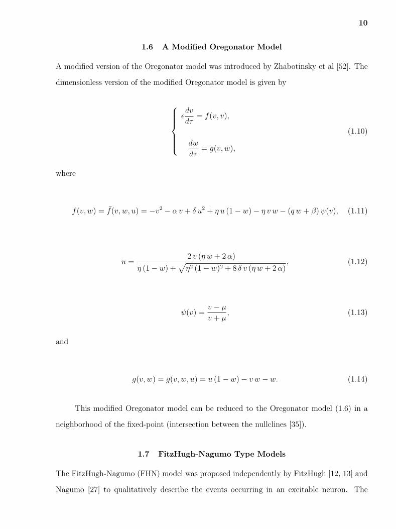
1.6 A Modified Oregonator Model
A modified version of the Oregonator model was introduced by Zhabotinsky et al [52]. The
dimensionless version of the modified Oregonator model is given by
εdv
dτ= f(v, v),
dw
dτ= g(v, w),
(1.10)
where
f(v, w) = f(v, w, u) = −v2 − α v + δ u2 + η u (1− w)− η v w − (q w + β) ψ(v), (1.11)
u =2 v (η w + 2 α)
η (1− w) +√
η2 (1− w)2 + 8 δ v (η w + 2 α), (1.12)
ψ(v) =v − µ
v + µ, (1.13)
and
g(v, w) = g(v, w, u) = u (1− w)− v w − w. (1.14)
This modified Oregonator model can be reduced to the Oregonator model (1.6) in a
neighborhood of the fixed-point (intersection between the nullclines [35]).
1.7 FitzHugh-Nagumo Type Models
The FitzHugh-Nagumo (FHN) model was proposed independently by FitzHugh [12, 13] and
Nagumo [27] to qualitatively describe the events occurring in an excitable neuron. The

11
FHN model is a generic model for excitable media and has been used as a caricature model
in a variety of systems, most notably chemistry biology and neuroscience [9]. The precise
mathematical mechanism involves appearance and disappearance of a limit cycle attractor,
and it is reviewed in detail by Izhikevich [17]. Its fast-slow system version is able to describe
relaxation oscillations in some parameter regimes. These oscillations and the nullclines are
qualitatively similar to the ones displayed by the Oregonator model. For this reason the
FHN model can been used as a toy model for the BZ reaction (1.16). The general form of
the FHN model is
v′ = f(v)− w,
w′ = ε [ g(v; λ)− w ](1.15)
where
f(v) = −h v3 + a v2 − b v + c, (1.16)
and
g(v; λ) = α v − λ. (1.17)
with h, a, b, c and α non-negative constants, and 0 < ε ¿ 1. In the classical FHN model,
h = 1/3, a = 1, b = c = 0, so the cubic v-nullcline has a minimum at (0, 0), and intersects
the w-nullcline at this point.
A modified version of the FHN model where g(v; λ) is sigmoid rather than linear has
been used in [34] as a toy model for the modified Oregonator model. More specifically, the
w-nullcline for the modified FitzHugh-Nagumo (MFHN) model is given by

12
g(v; λ) = β
(tanh
v − λ
η
)+
1
2. (1.18)
where η, λ and β are non-negative constants.
−0.5 0 0.5 1 1.5−0.2
0
0.2
0.4
0.6
0.8
1
1.2
1.4
1.6
v
w
λ=0.01;ε=0.01;α=4
TrajectoryN
w(v)
Nv(v)
0 200 400 600 800 1000
−1
−0.5
0
0.5
1
1.5
2
t
λ=0.01;ε=0.01;α=4
vw
Figure 1.2 Phase-plane (left) and traces (right) for the FHN (1.15) for representativeparameter values.

CHAPTER 2
THE KURAMOTO MODEL
In the past decades, the synchronization in complex networks has been a research topic in
many fields [22]. Among many models that have been proposed to address synchronization
phenomena, one of the most successful models is the Kuramoto model [19]. This model can be
used to understand the emergence of synchronization in networks of oscillators. In particular,
this model presents a second-order phase transition from incoherence to synchronization.
Kuramoto found that there is a certain value of the coupling constant, KC , above which
synchronization can occur, and below which it cannot. For any distribution of the natural
frequencies of the oscillators, he was able to calculate KC . For example, for a Lorentzian
distribution of natural frequencies, KC is just equal to the full width at half-max of the
Lorentzian curve. For other distributions, the formula for KC is more complex, but we can
still calculate it.
In this section we first describe the history of Kuramoto model. Kuramoto also gave
an initial estimate for the value of order parameter for a given value of coupling constant.
i.e. He gave a initial estimate for the value of the order parameter by giving the value of
the coupling constant. But the numerical results for the value of the order parameter are
a little bit different from Kuramoto’s estimation. I gave an estimate for the distribution of
order parameter for different values of initial conditions.
In the 1960s, scientists began to build mathematical models for synchronization in
many natural systems. Particularly, Arthur Winfree’s model become very popular. He gave
a model in which each oscillator’s phase is determined by combining the state of all of the
oscillators. In his model, the rate of change of the phase of an oscillator is determined
by its own natural frequency ωi and the state of all of the other oscillators combined.
Each oscillator’s sensitivity to the combination is represented as a function Y, and its own
contribution to the combination is given by a function X. Then each oscillator has an equation
to describe how its phase changes [39, 40]:
13
14
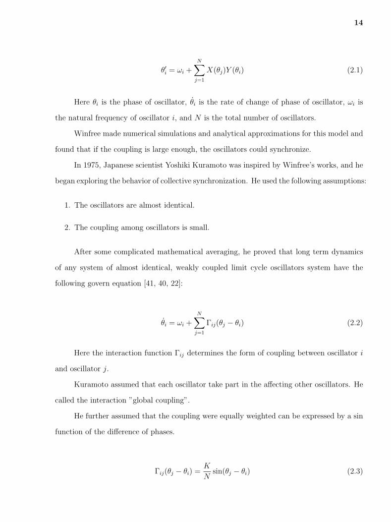
θ′i = ωi +N∑
j=1
X(θj)Y (θi) (2.1)
Here θi is the phase of oscillator, θi is the rate of change of phase of oscillator, ωi is
the natural frequency of oscillator i, and N is the total number of oscillators.
Winfree made numerical simulations and analytical approximations for this model and
found that if the coupling is large enough, the oscillators could synchronize.
In 1975, Japanese scientist Yoshiki Kuramoto was inspired by Winfree’s works, and he
began exploring the behavior of collective synchronization. He used the following assumptions:
1. The oscillators are almost identical.
2. The coupling among oscillators is small.
After some complicated mathematical averaging, he proved that long term dynamics
of any system of almost identical, weakly coupled limit cycle oscillators system have the
following govern equation [41, 40, 22]:
θi = ωi +N∑
j=1
Γij(θj − θi) (2.2)
Here the interaction function Γij determines the form of coupling between oscillator i
and oscillator j.
Kuramoto assumed that each oscillator take part in the affecting other oscillators. He
called the interaction ”global coupling”.
He further assumed that the coupling were equally weighted can be expressed by a sin
function of the difference of phases.
Γij(θj − θi) =K
Nsin(θj − θi) (2.3)

15
This derives the govern equations for Kuramoto model:
θ′i = ωi +K
N
N∑j=1
sin(θj − θi) (2.4)
Here K is the coupling constant, and N is the total number of oscillators. The model
assumed that N is very large, i.e large number of oscillators. The natural frequencies ωi
distributed by a probability density function g(ω), and it is symmetric about some value Π:
g(Π + ω) = g(Π− ω).
To simplify the governing equation of Kuramoto model, we need to define the order
parameter, the order parameter describes the ”mean field of the system”.
Let us write the governing equations of Kuramoto model in terms of order parameter:
reiψ =1
NΣN
j=1eiθj (2.5)
Here ψ is the average phase of all the oscillators.
2.1 The Relations between the Order Parameter r and the Critical Point Kc
The modulus of r, is a measure of the coherence of the oscillator system, it describes how
close the oscillators are together. If we increase the order parameter, the phases of the
oscillators will get closer together. The graphs in Fig. 2.1 show the order parameter being
an arrow pointing from the center of the circle.
Let us consider (2.5): Multiplying both sides by e−iθi we get:
rei(ψ−θi) =1
NΣN
j=1ei(θj−θi) (2.6)
r sin(ψ − θi) =1
NΣN
j=1 sin(θj − θi) (2.7)
Therefore, Equation (2.4) may be rewritten as

16
A
−1.5 −1 −0.5 0 0.5 1 1.5
−1
−0.5
0
0.5
1
r= 0.2490
−1.5 −1 −0.5 0 0.5 1 1.5
−1
−0.5
0
0.5
1
r= 0.6056
B
−1.5 −1 −0.5 0 0.5 1 1.5
−1
−0.5
0
0.5
1
r= 0.9413
−1.5 −1 −0.5 0 0.5 1 1.5
−1
−0.5
0
0.5
1
r= 0.9907
Figure 2.1 The order parameter is represented by the vector pointing from the center ofthe unit circle.

17
θi = ωi + Kr sin(ψ − θi) for i = 1, 2, ...N. (2.8)
The corresponding stationary density:
ρ =
δ[θ − ψ − sin−1( wKr
)] H(cos θ) when |ω| < Kr
C
|ω −Kr sin(θ − ψ)| when |ω| ≥ Kr
(2.9)
Here H(x) is the Heaviside unit step function.
We take the natural frequency density function to be the Lorentzian density, defined
as
g(ω) =γ
π(γ2 + ω2)(2.10)
Actually r(t) does not depend on time or ψ(t) and ψ(t) rotates uniformly at an angular
frequency φ. We can set up a frame of reference that is rotating at the same frequency. Hence
r(t) is stationary. So we can set ψ(t) to any constant value. Without loss of generality, set
ψ(t) ≡ 0 in the rotating frame. So we get
θi = ωi −Kr sin θi (2.11)
and correspondingly, the stationary density function is
ρ =
δ[θ − sin−1( wKr
)] H(cos θ), when |ω| < Kr
C
|ω −Kr sin θ| , when |ω| ≥ Kr
(2.12)

18
then
reiψ = rei0 = r
=1
NΣN
j=1eiθj =< eiθ >
=< eiθ >lock + < eiθ >unlock
According to (2.12)
ρ(θ + π,−ω) = ρ(θ, ω)
Compute the contribution of unlocked oscillators:
< eiθ >unlock =
∫ π
−π
∫ −Kr
−∞eiθρ(θ, ω)g(ω) dω dθ (2.13)
+
∫ π
−π
∫ ∞
Kr
eiθρ(θ, ω)g(ω) dω dθ
=I1 + I2
where
I1 =
∫ π
−π
∫ −Kr
−∞eiθρ(θ, ω)g(ω) dω dθ
= −∫ π
−π
∫ Kr
∞eiθρ(θ,−ω)g(−ω) dω dθ
Let θ′ = θ − π, then
I1 = −∫ 0
−2π
∫ Kr
∞eiθ′eiπρ(θ′ + π,−ω)g(−ω) dω dθ′
Since ρ(θ′ + π,−ω) = ρ(θ′, ω), g(−w) = g(w), eiπ = −1, we hence have
I1 = −∫ 0
−2π
∫ ∞
Kr
eiθ′eiπρ(θ′, ω)g(ω) dω dθ′
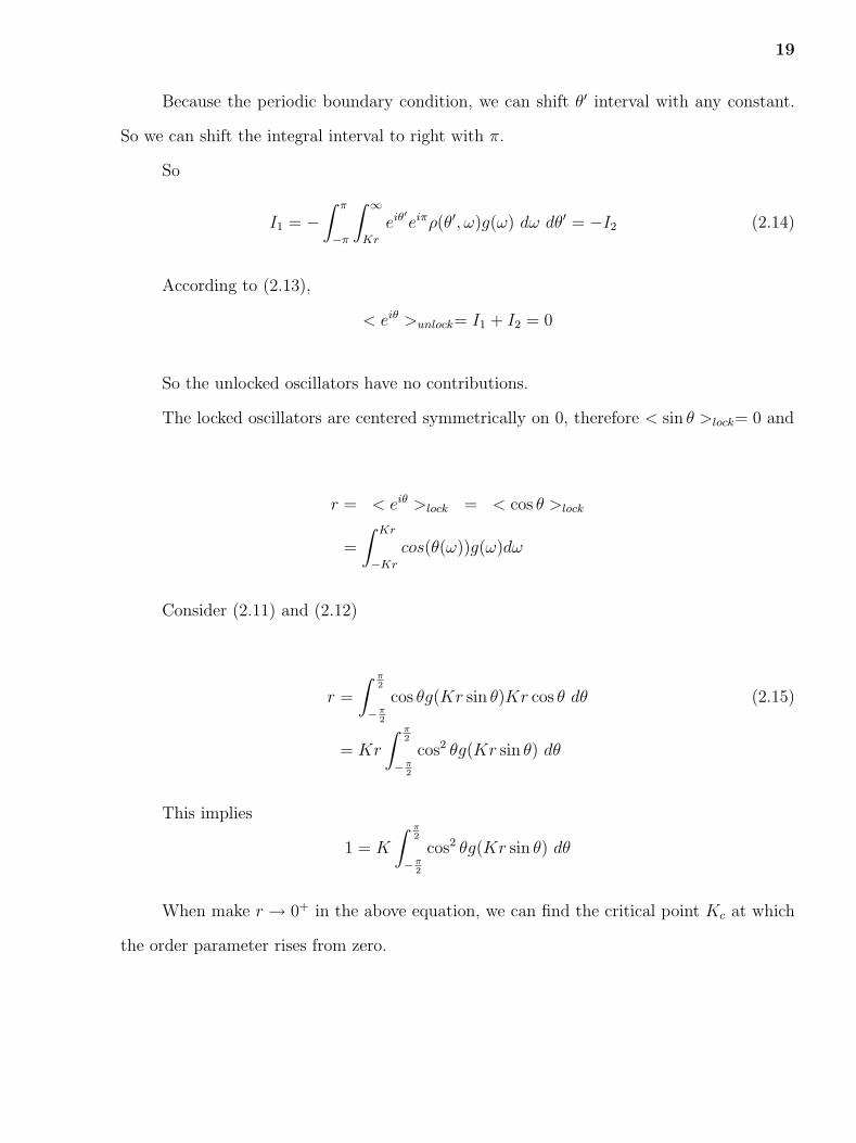
19
Because the periodic boundary condition, we can shift θ′ interval with any constant.
So we can shift the integral interval to right with π.
So
I1 = −∫ π
−π
∫ ∞
Kr
eiθ′eiπρ(θ′, ω)g(ω) dω dθ′ = −I2 (2.14)
According to (2.13),
< eiθ >unlock= I1 + I2 = 0
So the unlocked oscillators have no contributions.
The locked oscillators are centered symmetrically on 0, therefore < sin θ >lock= 0 and
r = < eiθ >lock = < cos θ >lock
=
∫ Kr
−Kr
cos(θ(ω))g(ω)dω
Consider (2.11) and (2.12)
r =
∫ π2
−π2
cos θg(Kr sin θ)Kr cos θ dθ (2.15)
= Kr
∫ π2
−π2
cos2 θg(Kr sin θ) dθ
This implies
1 = K
∫ π2
−π2
cos2 θg(Kr sin θ) dθ
When make r → 0+ in the above equation, we can find the critical point Kc at which
the order parameter rises from zero.

20
1 = Kc
∫ π/2
−π/2
cos2 θg(0) dθ
= Kcg(0)
∫ π/2
π/2
cos2 θ dθ = Kcg(0)π
2
Hence
Kc =2
πg(0)(2.16)
Plug in (2.10): the function of g(w)
1 = K
∫ π2
−π2
cos2 θγ
π(γ2 + K2r2 sin2 θ)dθ
=Kγ
π
∫ π2
−π2
1− sin2 θ
γ2 + K2r2 sin2 θdθ
= − γ
Kr2+
Kr
π(1 +
γ2
K2r2)
∫ π2
−π2
dθ
γ2 + K2r2 sin2 θ
= − γ
Kr2+ 2
Kr
π(1 +
γ2
K2r2)
∫ ∞
0
d(tan θ)
γ2 sec2 θ + K2r2 tan2 θ
= − γ
Kr2+ 2
Kr
π(1 +
γ2
K2r2)
∫ ∞
0
du
γ2(1 + u2) + K2r2u2
= − γ
Kr2+
√K2r2 + γ2
Kr2
Therefore we have
Kr2 = −γ +√
K2r2 + γ2
and hence
r =
√1− 2γ
K. (2.17)

21
To make the process of synchronization clear, the graphs Fig. 2.2 shows how the order
parameter r rises as the coupling K between oscillators is increased. Numerical curves are
taken from 500 oscillators with natural frequencies distributed with Lorentzian distribution:
0 1 2 3 4 5 60
0.1
0.2
0.3
0.4
0.5
0.6
0.7
0.8
0.9
1
K
|r|
Numerical and Theoretical curve of phase synchronization
Numerical curveTheoretical curve
Figure 2.2 Numerical curve and analytical curve for order parameter by changing K
g(ω) =γ
π(γ2 + ω2)
with γ = 0.5. Analytical curve is given by (2.17), according to (2.16), Kc = 1.
There is another way to visualize the synchronization: There are three graphs in Figure
2.3. The oscillators are numbered from the lowest to highest natural frequency, natural
frequencies also distributed by Lorentzian distribution.
g(ω) =γ
π(γ2 + ω2)
with γ = 0.5.

22
0 500 1000 1500 20000
1
2
3
4
5
6
oscillator n
phase θ
n
k=0.7; 2000 oscillators not synchronized
0 500 1000 1500 20000
1
2
3
4
5
6
oscillator n
phase θ
n
k=1; 2000 oscillators start to partially synchronized
0 500 1000 1500 20000
1
2
3
4
5
6
oscillator n
phase θ
n
k=1.5; 2000 oscillators partially synchronized
Figure 2.3 The synchronize phase θn of 2000 oscillators, take K=0.7, 1, 1.5

23
So
Kc =2
πg(0)= 1
, We can see obvious partial synchronization at or above Kc.
2.2 The Density Functions of Locked Terms and Unlocked Terms
To prove that the locked terms and unlocked terms are independent, we first try to get the
probability density function of locked terms and unlocked terms separately.
Suppose the probability density function of locked terms is f(y), then it satisfies the
following equation:
P (y ≤ cos θ ≤ y + dy| θ locked) = f(y) dy
P (arccos(y + dy) ≤ θ ≤ arccos y)
P (θ locked)= f(y) dy
For y > 0,
LHS =2P (sin(arccos(y + dy)) ≤ ω
kr≤ sin(arccos y))
P (θ locked)
This derives
P (θ locked) =
∫ kr
−kr
γ
π(γ2 + ω2)dω =
2
πarctan(
kr
γ)
24
P (sin(arccos(y + dy)) ≤ ω
kr≤ sin(arccos y)))
= P (kr sin(arccos(y + dy)) ≤ ω ≤ kr sin(arccos y))
= P (kr√
1− (y + dy)2 ≤ ω ≤ kr√
1− y2)
=
∫ kr√
1−y2
kr√
1−(y+dy)2
γ
π(γ2 + ω2)dω
=1
π
∫ krγ
√1−y2
krγ
√1−(y+dy)2
du
1 + u2
=1
π(arctan(
kr
γ
√1− y2)− arctan(
kr
γ
√1− (y + dy)2))
Let α = arctan(krγ
√1− y2)− arctan(kr
γ
√1− (y + dy)2)
As dy → 0, α → 0, α → tan α
So
α → tan α =
krγ
(√
1− y2 −√
1− (y + dy)2)
1 + (krγ
)2√
(1− y2)(1− (y + dy)2)
As dy → 0,
k r y dy
γ√
1− y2
1
1 + (kr/γ)2(1− y2)→ k ry γ
√1− y2 dy
γ2(1− y)2 + (kr(1− y2))2
This derives the density function: for 0 ≤ y ≤ 1,
f(y) =k r γ y
√1− y2
arctan(krγ
)(γ2(1− y2) + (kr(1− y2))2)
The density function of unlocked term satisfies:
P (y ≤ cos θ ≤ y + dy| θ unlocked) = f(y) dy
For 0 ≤ y ≤ 1, y ≤ cos θ ≤ y + dy.
So√
1− (y + dy)2 ≤ sin θ ≤√
1− y2, dθ = dy√1−y2

25
or −√
1− y2 ≤ sin θ ≤ −√
1− (y + dy)2, dθ = dy√1−y2
ρ(θ, ω) =C
|θ′| =C
|ω − kr sin θ|
So
1 =
∫ π
−π
ρ(θ, ω)dθ = C
∫ π
−π
dθ
|ω − kr sin θ|
Which derives
C =
√ω2 − (kr)2
2π
So
P (y ≤ cos θ ≤ y + dy|θ unlocked) =P (y ≤ cos θ ≤ y + dy, |ω| > kr)
P (|ω| > kr)
=P (−
√1− (y + dy)2 ≤ sin θ ≤ −
√1− y2, |ω| > kr)
P (|ω| > kr)
+P (−
√1− y2 ≤ sin θ ≤ −
√1− (y + dy)2, |ω| > kr)
P (|ω| > kr)
=
∫Ig(ω)
∫I1
ρ(θ, ω)dθdω +∫
Ig(ω)
∫I2
ρ(θ, ω)dθdω
2∫∞
krγ
π(γ2+ω2)dω
A1 =
∫
I
g(ω)
∫
I1
ρ(θ, ω)dθdω
=1
2π
∫
I
γ
π(γ2 + ω2)
∫
I1
√ω2 − (kr)2
|ω − kr√
1− y2|dθdω
=1
2π2
∫
I
γ
γ2 + ω2
∫
I1
√ω2 − (kr)2
|ω − kr√
1− y2|dy√1− y2
dω

26
As dy → 0, dθ → 0, I1 → 0, I2 → 0
A1 → 1
2π2(
∫
I
γ
γ2 + ω2
√ω2 − (kr)2
ω − kr√
1− y2
1√1− y2
dω)dy
=1
2π2√
1− y2
∫
I
γ
γ2 + ω2
√ω2 − (kr)2
|ω − kr√
1− y2|dωdy
A2 =
∫
I
∫
I2
g(ω)ρ(θ, ω)dθdω
=1
2π2
∫
I
∫
I2
1√1− y2
γ
γ2 + ω2
√ω2 − (kr)2
|ω + kr√
1− y2|dydω
= (1
2π2√
1− y2
∫
I
γ
γ2 + ω2
√ω2 − (kr)2
|ω + kr√
1− y2|dω)dy
This derives
A1 + A2 =1
2π2√
1− y2(
∫
I
γ√
ω2 − (kr)2
γ2 + ω2(
1
|ω + kr√
1− y2| +1
|ω − kr√
1− y2|))dωdy
Similarly, for −1 ≤ y < 0,
A1 + A2 =1
2π2√
1− y2
∫
I
γ√
ω2 − (kr)2
γ2 + ω2(
1
|ω + kr√
1− y2| +1
|ω − kr√
1− y2|)dωdy
=γ
2π2√
1− y2
∫
I
√ω2 − (kr)2
γ2 + ω2
2|ω|ω2 − (kr)2(1− y2)
dωdy
=2γ
π2√
1− y2
∫ ∞
kr
ω√
ω2 − (kr)2
(γ2 + ω2)(ω2 − (kr)2(1− y2))dωdy
=γ
π2√
1− y2
∫ ∞
α
√t− α
(t + γ2)(t− α(1− y2))dtdy
=γ
π2√
1− y2
∫ ∞
0
√t
(t + α + γ2)(t + αy2)dtdy
⇒
27
P (y ≤ cos θ ≤ y + dy, |ω| > kr)
P (|ω| > kr)= f(y)dy
=γ
π2√
1− y2
1
1− 2πarctan(kr
γ)
∫ ∞
0
√tdtdy
(t + α + γ2)(t + αy2)
=γ
π√
1− y2
1
π − 2arctan(krγ
)
∫ ∞
0
√tdtdy
(t + α + γ2)(t + αy2)
⇒
f(y) =γ
π√
1− y2(π − 2 arctan(kr/γ))
∫ ∞
0
√tdt
(t + α + γ2)(t + αy2)
=γ√
1− y2(π − 2arctan(kr/γ))
1√α + γ2 +
√αy2
=γ√
1− y2(π − 2arctan(kr/γ))
1√(kr)2 + γ2 + kr|y|
So we have the density function f for locked part and f for unlocked part:
f(y) =k r γ y
√1− y2
arctan(krγ
)(γ2(1− y2) + (kr(1− y2))2)(2.18)
f(y) =γ√
1− y2(π − 2arctan(kr/γ))(√
(kr)2 + γ2 + kr|y|) (2.19)
To prove the locked terms are independent, we want to show that the sum of any two
locked terms satisfies the analytical probability density function derived by convolution law:
If X and Y are two locked terms, Z is the sum of X and Y:
Z = X + Y
28
E(etZ) =
∫ ∞
−∞etufz(u)du (2.20)
=
∫ ∞
−∞
∫ ∞
−∞etxetyfx(x)fy(y)dxdu (2.21)
=
∫ ∞
−∞etu
∫ ∞
−∞fx(x)fy(u− x)dxdu (2.22)
⇒
fz(u) =
∫ ∞
−∞fx(x)fy(u− x)dx
Similarly, to prove the unlocked terms are independent, we can also get the analytical
probability density function of two unlocked terms by the convolution law:
If X and Y are two unlocked terms, Z is the sum of X and Y :
Z = X + Y
E(etz) =
∫ ∞
−∞etufz(u)du (2.23)
=
∫ ∞
−∞
∫ ∞
−∞etxetyfx(x)fy(y)dxdu (2.24)
=
∫ ∞
−∞etu
∫ ∞
−∞fx(x)fy(u− x)dxdu (2.25)
⇒
fz(u) =
∫ ∞
−∞fx(x)fy(u− x)dx
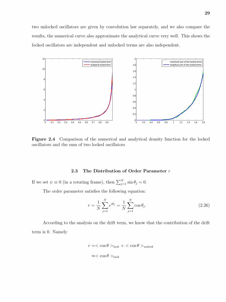
In the following figures, we compare the numerical and analytical result for the density
functions, the numerical result of density function for one oscillator satisfies the analytical
result very well. The analytical density function of the sum of two locked oscillators and
29
two unlocked oscillators are given by convolution law separately, and we also compare the
results, the numerical curve also approximate the analytical curve very well. This shows the
locked oscillators are independent and unlocked terms are also independent.
0 0.1 0.2 0.3 0.4 0.5 0.6 0.7 0.8 0.90
2
4
6
8
10
12
numerical locked termanalytical locked term
0 0.2 0.4 0.6 0.8 1 1.2 1.4 1.6 1.80
0.2
0.4
0.6
0.8
1
1.2
1.4
1.6
1.8
2
numerical sum of two locked termsanalytical sum of two locked terms
Figure 2.4 Comparison of the numerical and analytical density function for the lockedoscillators and the sum of two locked oscillators
2.3 The Distribution of Order Parameter r
If we set ψ ≡ 0 (in a rotating frame), then∑N
j=1 sin θj = 0.
The order parameter satisfies the following equation:
r =1
N
N∑j=1
eiθj =1
N
N∑j=1
cos θj. (2.26)
According to the analysis on the drift term, we know that the contribution of the drift
term is 0. Namely
r =< cos θ >lock + < cos θ >unlock
≈< cos θ >lock

30
−1 −0.8 −0.6 −0.4 −0.2 0 0.2 0.4 0.6 0.8 10.2
0.4
0.6
0.8
1
1.2
1.4
1.6
1.8
2
numericalanalytical
−2 −1.5 −1 −0.5 0 0.5 1 1.5 20
0.1
0.2
0.3
0.4
0.5
0.6
0.7
0.8
Figure 2.5 Comparison of the numerical and analytical density function for the unlockedoscillators and the sum of two unlocked oscillators
There are totally N terms θ1, θ2, ...θN . Without loss of generality, we suppose the
first n terms θ1, θ2, ...θn are synchronized, and the last N − n terms θn+1, θn+2, ...θN are not
synchronized. Here 0 < n < N.
From equation (2.26), we get
r =1
N
N∑j=1
eiθj =1
N
N∑j=1
cos θj (2.27)
=1
N
n∑j=1
cos θj +1
N
N∑j=n+1
cos θj
Suppose S1 =∑n
j=1 cos θj, S2 =∑N
j=n+1 cos θj, S =∑N
j=1 cos θj,
then
S1 + S2 = S = Nr
and
S2 ≈ 0, S1 ≈ S = Nr
.

31
For a fixed number N, if we also fix a series of natural frequency ω1, ω2, ...ωN , and these
series of natural frequency satisfies the Lorentzian distribution very well-proportionally, the
density function is
g(ω) =ν
π(ν2 + ω2)
.
Take different series of initial values of θj, j = 1, 2, ...N .
These series of θj are taken randomly which satisfy uniformly distribution. We will get
different values of order parameter r for each series of θj, j = 1, 2, ...N .
Question: When the value of N is very large, what is the distribution of the value of
order parameter r?
When N is large, n and N-n are large. According to central limit theorem,
S1 − nµ1
σ1
√n
∼ N(0, 1)
. Here µ1 and σ1 are the mean and variance of locked terms cos θj, j = 1, 2, ...n.
S2 − (N − n)µ2
σ2
√N − n
∼ N(0, 1)
Here µ2 and σ2 are the mean and variance of unlocked terms cos θj, j = n + 1, n + 2, ...N
We know that S1 and S2 both satisfy Gaussian distribution. From equation (2.27) the
order parameter
r =1
N(S1 + S2)
is the linear combination of Gaussian distributed functions. So r also satisfies Gaussian
distribution. The variance of S1 is σ21n and the variance of S2 is σ2
2(N − n),
σ satisfies the following equation:
σ =1
N2(σ2
1n + σ22(N − n))
32
.
So the question is reduced to calculate the value of σ1 and σ2.
σ1 is the variance of locked terms cos θ1, cos θ2, ..., cos θn.
σ1 = V ar(θ)locked = E(cos2 θ)locked − (E(cos θ)locked)2
E(cos2 θ)locked =
∫ π2
−π2cos2 θg(Kr sin θ)Kr cos θ dθ
∫ π2
−π2g(Kr sin θ)Kr cos θ dθ
(2.28)
Here
∫ π2
−π2
cos2 θg(Kr sin θ)Kr cos θ dθ =Krν
π
∫ π2
−π2
cos3 θ
ν2 + K2r2 sin2 θdθ
=2ν
πKr(ν2 + K2r2
Krνarctan(
Kr
ν)− 1)
∫ π2
−π2
g(Kr sin θ)Kr cos θ dθ =Krν
π
∫ π2
−π2
cos θ
ν2 + K2r2 sin2 θdθ
=2
πarctan(
Kr
ν)
Plug these results into the equation (2.28), we can get
E(cos2 θ)locked =ν
Kr(ν2 + K2r2
Krν− 1
arctan(Krν
)) (2.29)
The variance of unlocked terms is
σ2 = V ar(θ)unlocked = E(cos2 θ)unlocked − (E(cos θ)unlocked)2

33
E(cos2 θ)unlocked =
∫ π/2
−π/2
∫
|ω|>Kr
cos2 θCg(ω)
|ω −Kr sin θ| dθ dω
= 2
∫ π/2
−π/2
∫
ω>Kr
cos2 θCg(ω)
|ω −Kr sin θ| dθ dω
and
E(cos θ)unlocked =
∫ π/2
−π/2
∫
|ω|>Kr
cos θCg(ω)
|ω −Kr sin θ| dθ dω
= 2
∫ π/2
−π/2
∫
ω>Kr
cos θCg(ω)
|ω −Kr sin θ| dθ dω
Here g(ω) = νπ(ν2+ω2)
, C =√
ω2−K2r2
2π.
These integrals are relatively hard to simplify, but we can use numerical methods to
get the variance of the unlocked terms.
The variance of order parameter r is σ = 1N2 (σ
21n + σ2
2(N − n)).
i.e
r −mean(r)1N
√σ2
1n + σ22(N − n)
∼ N(0, 1) (2.30)
Taking 1000 series of uniformly distributed initial values θ1, θ2, ... θN , we can get
1000 values of order parameter r. The order parameter r approximately satisfies Gaussian
distribution, the equation for this distribution is (2.30).
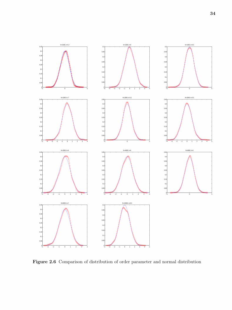
The graphs in Figure 2.6 compare the LHS of (2.30) with N(0, 1) (standard normal
distribution). The blue line is the density function of standard normal distribution, the red
line is the density function of the distribution of LHS function.
34
−5 0 50
0.05
0.1
0.15
0.2
0.25
0.3
0.35
0.4
0.45N=1000, k=5.2
−5 −4 −3 −2 −1 0 1 2 3 40
0.05
0.1
0.15
0.2
0.25
0.3
0.35
0.4N=1000, k=6
−5 0 50
0.05
0.1
0.15
0.2
0.25
0.3
0.35
0.4N=1000, k=6.5
−5 −4 −3 −2 −1 0 1 2 3 40
0.05
0.1
0.15
0.2
0.25
0.3
0.35
0.4
0.45N=1000, k=7
−5 0 50
0.05
0.1
0.15
0.2
0.25
0.3
0.35
0.4
0.45N=2000, k=5.2
−4 −3 −2 −1 0 1 2 3 4 50
0.05
0.1
0.15
0.2
0.25
0.3
0.35
0.4
0.45N=2000, k=5.5
−4 −3 −2 −1 0 1 2 3 40
0.05
0.1
0.15
0.2
0.25
0.3
0.35
0.4
0.45N=2000, k=6
−4 −3 −2 −1 0 1 2 3 40
0.05
0.1
0.15
0.2
0.25
0.3
0.35
0.4
0.45N=4000, k=6
−5 0 50
0.05
0.1
0.15
0.2
0.25
0.3
0.35
0.4
0.45N=6000, k=6
−4 −3 −2 −1 0 1 2 3 40
0.05
0.1
0.15
0.2
0.25
0.3
0.35
0.4
0.45N=6000, k=7
−4 −3 −2 −1 0 1 2 3 4 50
0.05
0.1
0.15
0.2
0.25
0.3
0.35
0.4N=10000, k=5.5
Figure 2.6 Comparison of distribution of order parameter and normal distribution

CHAPTER 3
OSCILLATORY CLUSTERS IN THE BZ REACTION
Physicochemical systems with coupled processes on different length scales often exhibit
stationary spatially periodic structures [35]. The photosensitive BZ reaction has proven
to be an ideal model system for studies of perturbed excitable media. Numerical simulations
of chaotic states in some low dimensional models are carried out and novel structures of the
first return maps representitive of BZ chaos in a three-variable model are discovered [44].
The FitzHugh-Nagumo model [42],[23] is a generic model for excitable media and can be
applied to a variety of systems. FitzHugh called this simplified model the Bon Hoeffer-van der
Pol model and derived it in the 1960’s as a simplification of the Hodgkin-Huxley equations.
In this chapter, first I will introduce the Oregonator and FHN type models. The classic
FHN model has a cubic shaped function in the inhibitory term, but I used the piecewise
linear function to approximate the cubic term. The piecewise linear system has the same
shape as the cubic oscillators system for most of the parameters. It’s a good method to use
piecewise linear model to approximate the cubic FHN model.
3.1 Oscillatory Clusters in the Oregonator and FHN type Models with Global
Inhibitory Feedback
The modified Oregonator model (1.10) introduced in [52] with diffusion terms added to both
the activator and the inhibitor equations has been extended by Yang et al. to include global
feedback. This model reproduces the experimentally observed stable localized, two-phase
and three-phase clusters referred to above. The following global feedback term
γ(< w > −w)ψ(v) (3.1)
Here ψ(v) is defined in 1.13.
35
36
was added to the activator (v) equation. In (1.7), < w > represents the instantaneous spatial
average of the activator variable w, and w represents the target value of the oxidized form
of the catalyst, which was set equal to the unstable steady state concentration (unstable
fixed-point). The parameter γ is the global feedback coefficient, which depends on the
maximum actinic light intensity and on the quantum yield of the photochemical reaction.
Note that the global feedback represents the global effect of the inhibitor on the activator
rather than the global effect of the activator onto itself as is commonly encountered.[49]
The modified Oregonator model with global inhibitory feedback in the absence of
diffusion reads
ε1 dvkdτ = f(vk, wk)− γ (< w > −w) ψ(vk),
dwk/dτ = g(vk, wk),(3.2)
for k = 1, . . . , N , where f(v, w) and g(v, w) are given by (1.11) and (1.14) respectively, γ is
the global feedback parameter, ψ(vk) is defined in 1.13.
In a subsequent study, Rotstein et al. [35, 34] studied a mechanism of localized cluster
formation in the modified Oregonator model and in a model of FitzHugh-Nagumo type [34]
with global inhibitory feedback and no diffusion. If the system has N oscillators, the global
feedback term reads
< w > =1
N
N∑
k=1
wk. (3.3)
The parameter w is the w-coordinate of the intersection point between the nullclines when
γ = 0. Note that the intersection point between nullsurfaces does not change with γ.
In these studies a “cluster simplification” was made. By assuming that all oscillators in a
cluster have the same amplitude and frequency, all the oscillators belonging to the same
cluster are indistinguishable from the dynamic point of view, and can be described by the
37
same equations. Thus, a system of N globally coupled oscillators having M clusters can be
described by the following globally coupled system of M -oscillators
v′k = f(vk)− wk − γ [ < w > −w ],
w′k = ε [ g(vk; λ)− wk ],
(3.4)
for k = 1, . . . , M with
< w > =M∑
k=1
αk wk (3.5)
where αk, k = 1, . . . , M is the fraction of oscillators belonging to each cluster, note that∑n
k=1 αk = 1.
If M = 1, single oscillator system reads:
v′ = f(v)− (1 + γ)w − w ],
w′ = ε [αv − λ− w ](3.6)
If M = 2 (two clusters) sytem (3.4) reads
v′k = f(vk)− wk − γ [ α1 w1 + α2 w2 − w ],
w′k = ε [αvk − λ− wk ]
(3.7)
for k = 1, 2. This is a system of two oscillators globally coupled through the inhibitor
variables w1 and w2. Where the function f is given by (1.16). Here we have chosen h = 2
and a = 3, the result of making v′1 = v′2 = w′1 = w′
2 = 0 are not one-dimensional curves but
higher dimensional objects. In particular, by making v′k = 0 for k = 1, 2 one gets
wk =f(vk) + γ w
1 + αkγ− γ αjwj
1 + αkγ(3.8)
38
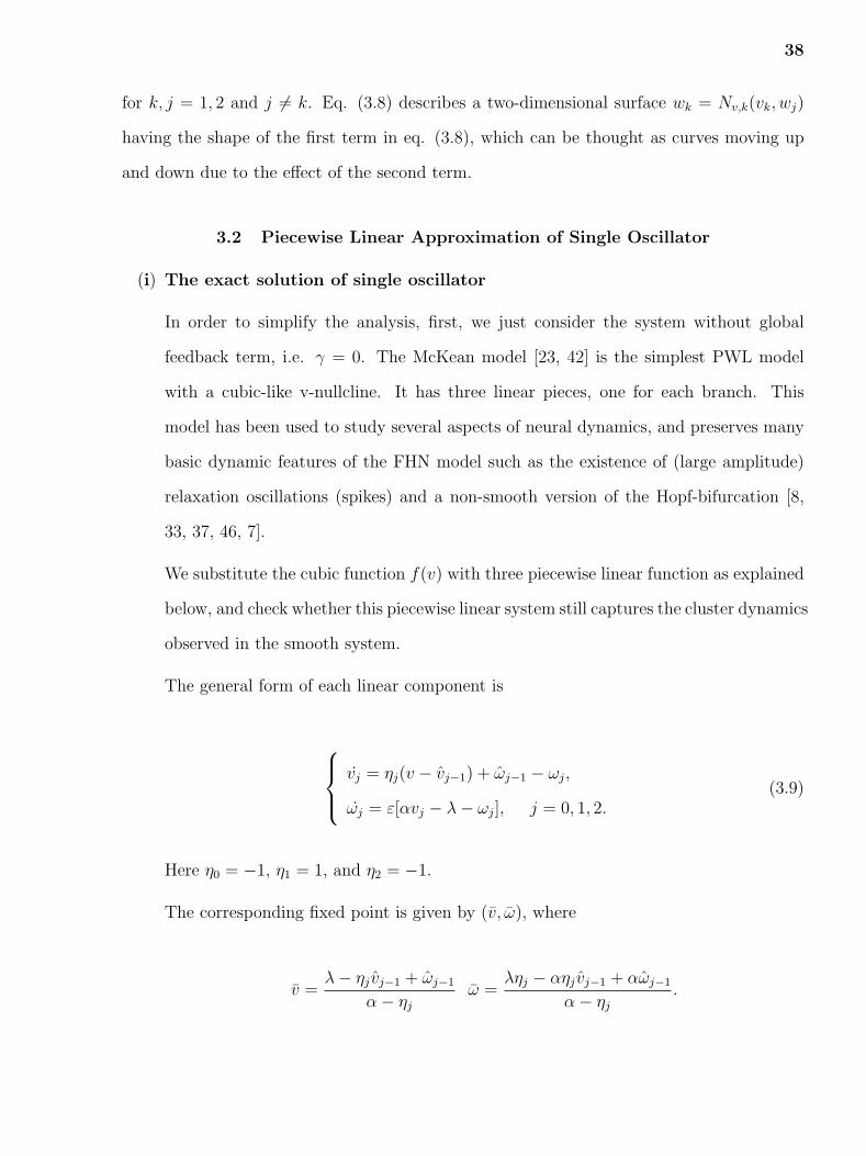
for k, j = 1, 2 and j 6= k. Eq. (3.8) describes a two-dimensional surface wk = Nv,k(vk, wj)
having the shape of the first term in eq. (3.8), which can be thought as curves moving up
and down due to the effect of the second term.
3.2 Piecewise Linear Approximation of Single Oscillator
(i) The exact solution of single oscillator
In order to simplify the analysis, first, we just consider the system without global
feedback term, i.e. γ = 0. The McKean model [23, 42] is the simplest PWL model
with a cubic-like v-nullcline. It has three linear pieces, one for each branch. This
model has been used to study several aspects of neural dynamics, and preserves many
basic dynamic features of the FHN model such as the existence of (large amplitude)
relaxation oscillations (spikes) and a non-smooth version of the Hopf-bifurcation [8,
33, 37, 46, 7].
We substitute the cubic function f(v) with three piecewise linear function as explained
below, and check whether this piecewise linear system still captures the cluster dynamics
observed in the smooth system.
The general form of each linear component is
vj = ηj(v − vj−1) + ωj−1 − ωj,
ωj = ε[αvj − λ− ωj], j = 0, 1, 2.(3.9)
Here η0 = −1, η1 = 1, and η2 = −1.
The corresponding fixed point is given by (v, ω), where
v =λ− ηj vj−1 + ωj−1
α− ηj
ω =ληj − αηj vj−1 + αωj−1
α− ηj
.

39
For simplicity, we make change of variables with the goal of shifting the fixed point to
the origin to study the dynamics in each linear regime.
−1 −0.5 0 0.5 1 1.5 2−0.2
0
0.2
0.4
0.6
0.8
1
1.2
1.4
1.6
1.8
v
w
λ=0.01;ε=0.01;α=4
TrajectoryN
w(v)
Nv(v)
0 200 400 600 800 1000
−1
−0.5
0
0.5
1
1.5
2
t
λ=0.01;ε=0.01;α=4
vw
Figure 3.1 Phase-plane (left) and traces (right) for the piecewise-linear approximation ofFHN (3.9) for representative parameter values.
Let us consider V := v − v and W := ω − ω with the following equation
V ′ = ηV −W, V (0) = v0 − v
W ′ = ε[αV −W ], W (0) = ω0 − ω
The Jacobian matrix of the above piecewise linear equation is
J =
η −1
εα −ε
whose eigenvalues are:
r1,2 =η − ε±
√(η − ε)2 − 4ε(α− η)
2
The fixed point is stable (unstable) if η < (>) ε. The eigenvalues are complex if
η ∈ (−ε− 2√
εα,−ε + 2√
εα).
40
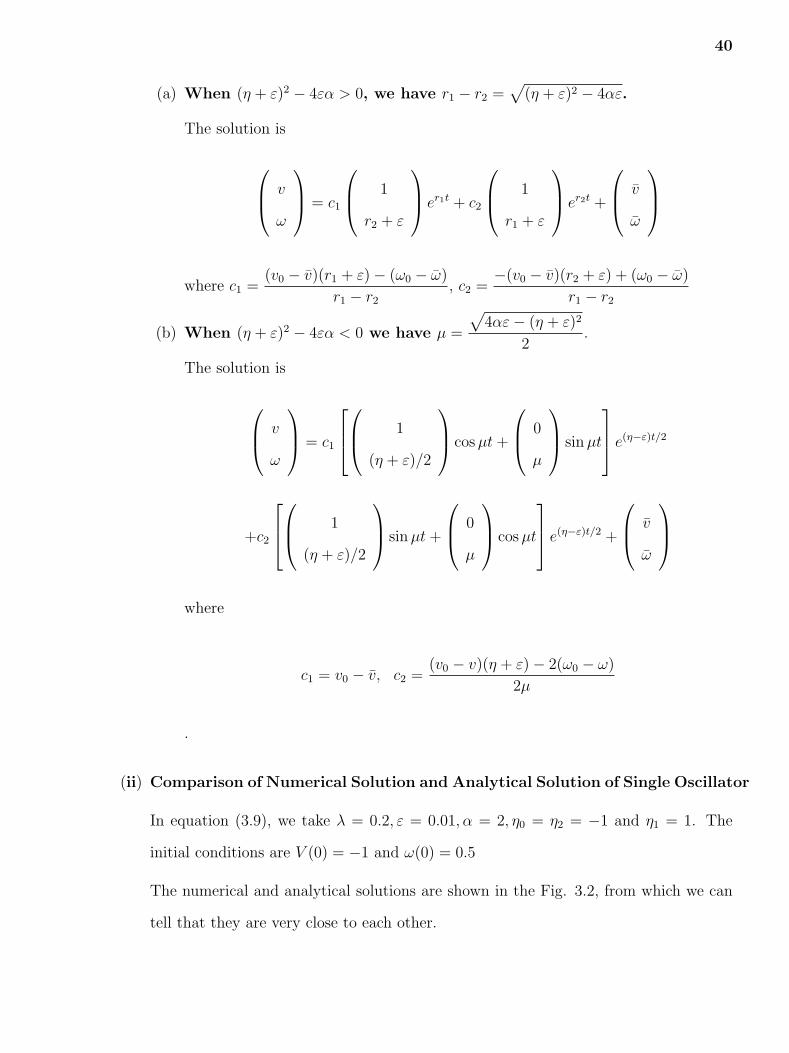
(a) When (η + ε)2 − 4εα > 0, we have r1 − r2 =√
(η + ε)2 − 4αε.
The solution is
v
ω
= c1
1
r2 + ε
er1t + c2
1
r1 + ε
er2t +
v
ω
where c1 =(v0 − v)(r1 + ε)− (ω0 − ω)
r1 − r2
, c2 =−(v0 − v)(r2 + ε) + (ω0 − ω)
r1 − r2
(b) When (η + ε)2 − 4εα < 0 we have µ =
√4αε− (η + ε)2
2.
The solution is
v
ω
= c1
1
(η + ε)/2
cos µt +
0
µ
sin µt
e(η−ε)t/2
+c2
1
(η + ε)/2
sin µt +
0
µ
cos µt
e(η−ε)t/2 +
v
ω
where
c1 = v0 − v, c2 =(v0 − v)(η + ε)− 2(ω0 − ω)
2µ
.
(ii) Comparison of Numerical Solution and Analytical Solution of Single Oscillator
In equation (3.9), we take λ = 0.2, ε = 0.01, α = 2, η0 = η2 = −1 and η1 = 1. The
initial conditions are V (0) = −1 and ω(0) = 0.5
The numerical and analytical solutions are shown in the Fig. 3.2, from which we can
tell that they are very close to each other.

41
A
0 200 400 600 800 1000−1
−0.5
0
0.5
1
1.5
2
t
V
Numerical solutionExact solution
0 200 400 600 800 1000−0.2
0
0.2
0.4
0.6
0.8
1
1.2
t
W
Numerical solutionExact solution
0 200 400 600 800 10000
0.02
0.04
0.06
0.08
0.1
t
Err
or o
f V
0 200 400 600 800 10000
0.5
1
1.5
2
2.5x 10
−3
t
Err
or o
f W
B
0 200 400 600 800 1000−1
−0.5
0
0.5
1
1.5
2
t
V
Numerical solutionExact solution
0 200 400 600 800 1000−0.2
0
0.2
0.4
0.6
0.8
1
1.2
t
W
Numerical solutionExact solution
0 200 400 600 800 10000
0.01
0.02
0.03
0.04
0.05
t
Err
or o
f V
0 200 400 600 800 1000−5
0
5
10
15x 10
−3
t
Err
or o
f W

42
C
0 200 400 600 800 1000−1
−0.5
0
0.5
1
1.5
2
t
V
Numerical solutionExact solution
0 200 400 600 800 1000−0.2
0
0.2
0.4
0.6
0.8
1
1.2
tW
Numerical solutionExact solution
0 200 400 600 800 10000
0.01
0.02
0.03
0.04
0.05
t
Err
or o
f V
0 200 400 600 800 10000
0.002
0.004
0.006
0.008
0.01
0.012
t
Err
or o
f W
Figure 3.2 Comparison between the analytical and numerical solutions for a single PWLoscillator evolving according to eq. (3.8) with α = 2, ε = 0.01 and A λ = 0.01, B: λ = 0.1,and C: λ = 0.2. The cubic-like PWL function f(v) is given by (3.10) with β1 = β2 = 1. Foreach value of λ, the numerical (V ,dashed-red) and analytical (V , dashed-blue) solutions arepresented in the top panels. The corresponding absolute errors, defined as |V (t)− V (t)| and|W (t) − W (t)| presented in the bottom panels. The numerical and analytical solutions arein good agreement.

43
A
0 200 400 600 800 1000−1
−0.5
0
0.5
1
1.5
2
t
V
Numerical solutionExact solution
0 200 400 600 800 1000−0.2
0
0.2
0.4
0.6
0.8
1
1.2
t
W
Numerical solutionExact solution
0 200 400 600 800 10000
0.01
0.02
0.03
0.04
0.05
t
Err
or o
f V
0 200 400 600 800 10000
1
2
3
4
5
6x 10
−3
t
Err
or o
f W
B
0 200 400 600 800 1000−1
−0.5
0
0.5
1
1.5
2
t
V
Numerical solutionExact solution
0 200 400 600 800 1000−0.2
0
0.2
0.4
0.6
0.8
1
1.2
t
W
Numerical solutionExact solution
0 200 400 600 800 10000
0.005
0.01
0.015
0.02
0.025
t
Err
or o
f V
0 200 400 600 800 10000
0.2
0.4
0.6
0.8
1
1.2
1.4
1.6x 10
−3
t
Err
or o
f W
44
C
0 200 400 600 800 1000−1
−0.5
0
0.5
1
1.5
2
t
V
Numerical solutionExact solution
0 200 400 600 800 1000−0.2
0
0.2
0.4
0.6
0.8
1
1.2
tW
Numerical solutionExact solution
0 200 400 600 800 10000
0.01
0.02
0.03
0.04
0.05
t
Err
or o
f V
0 200 400 600 800 10000
1
2
3
4
5
6x 10
−3
t
Err
or o
f W
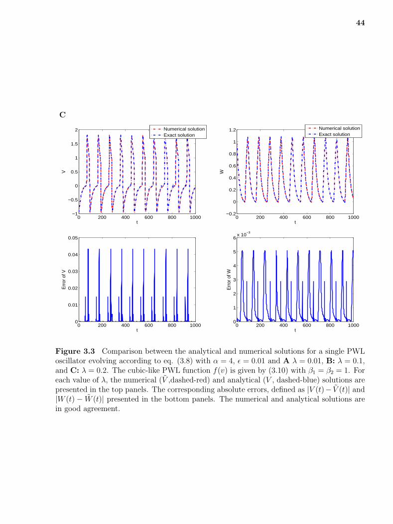
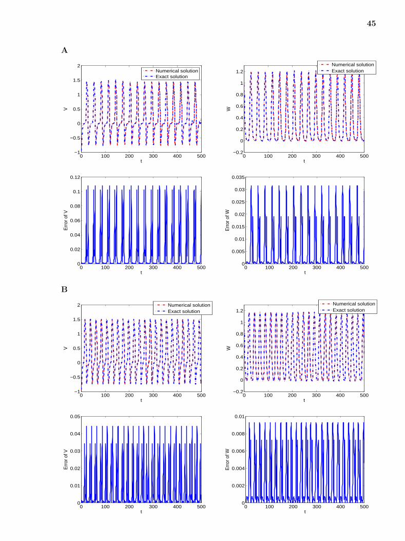
Figure 3.3 Comparison between the analytical and numerical solutions for a single PWLoscillator evolving according to eq. (3.8) with α = 4, ε = 0.01 and A λ = 0.01, B: λ = 0.1,and C: λ = 0.2. The cubic-like PWL function f(v) is given by (3.10) with β1 = β2 = 1. Foreach value of λ, the numerical (V ,dashed-red) and analytical (V , dashed-blue) solutions arepresented in the top panels. The corresponding absolute errors, defined as |V (t)− V (t)| and|W (t) − W (t)| presented in the bottom panels. The numerical and analytical solutions arein good agreement.
45
A
0 100 200 300 400 500−1
−0.5
0
0.5
1
1.5
2
t
V
Numerical solutionExact solution
0 100 200 300 400 500−0.2
0
0.2
0.4
0.6
0.8
1
1.2
t
W
Numerical solutionExact solution
0 100 200 300 400 5000
0.02
0.04
0.06
0.08
0.1
0.12
t
Err
or o
f V
0 100 200 300 400 5000
0.005
0.01
0.015
0.02
0.025
0.03
0.035
t
Err
or o
f W
B
0 100 200 300 400 500−1
−0.5
0
0.5
1
1.5
2
t
V
Numerical solutionExact solution
0 100 200 300 400 500−0.2
0
0.2
0.4
0.6
0.8
1
1.2
t
W
Numerical solutionExact solution
0 100 200 300 400 5000
0.01
0.02
0.03
0.04
0.05
t
Err
or o
f V
0 100 200 300 400 5000
0.002
0.004
0.006
0.008
0.01
t
Err
or o
f W

46
C
0 100 200 300 400 500−1
−0.5
0
0.5
1
1.5
2
t
V
Numerical solutionExact solution
0 100 200 300 400 500−0.2
0
0.2
0.4
0.6
0.8
1
1.2
tW
Numerical solutionExact solution
0 100 200 300 400 5000
0.005
0.01
0.015
0.02
0.025
0.03
0.035
t
Err
or o
f V
0 100 200 300 400 5000
0.002
0.004
0.006
0.008
0.01
t
Err
or o
f W
Figure 3.4 Comparison between the analytical and numerical solutions for a single PWLoscillator evolving according to eq. (3.8) with α = 2, ε = 0.1 and A λ = 0.01, B: λ = 0.1,and C: λ = 0.2. The cubic-like PWL function f(v) is given by (3.10) with β1 = β2 = 1. Foreach value of λ, the numerical (V ,dashed-red) and analytical (V , dashed-blue) solutions arepresented in the top panels. The corresponding absolute errors, defined as |V (t)− V (t)| and|W (t) − W (t)| presented in the bottom panels. The numerical and analytical solutions arein good agreement.

47
A
0 100 200 300 400 500−1
−0.5
0
0.5
1
1.5
2
t
V
Numerical solutionExact solution
0 100 200 300 400 500−0.2
0
0.2
0.4
0.6
0.8
1
1.2
1.4
t
W
Numerical solutionExact solution
0 100 200 300 400 5000
0.02
0.04
0.06
0.08
0.1
0.12
0.14
0.16
t
Err
or o
f V
0 100 200 300 400 5000
0.01
0.02
0.03
0.04
0.05
t
Err
or o
f W
B
0 100 200 300 400 500−1
−0.5
0
0.5
1
1.5
2
t
V
Numerical solutionExact solution
0 100 200 300 400 500−0.2
0
0.2
0.4
0.6
0.8
1
1.2
1.4
t
W
Numerical solutionExact solution
0 100 200 300 400 5000
0.01
0.02
0.03
0.04
0.05
0.06
0.07
0.08
t
Err
or o
f V
0 100 200 300 400 5000
0.005
0.01
0.015
0.02
0.025
0.03
t
Err
or o
f W
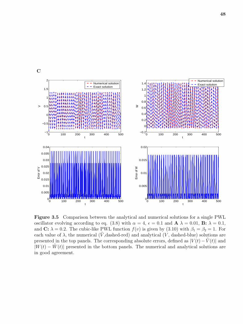
48
C
0 100 200 300 400 500−1
−0.5
0
0.5
1
1.5
2
t
V
Numerical solutionExact solution
0 100 200 300 400 500−0.2
0
0.2
0.4
0.6
0.8
1
1.2
1.4
tW
Numerical solutionExact solution
0 100 200 300 400 5000
0.005
0.01
0.015
0.02
0.025
0.03
0.035
0.04
t
Err
or o
f V
0 100 200 300 400 5000
0.005
0.01
0.015
0.02
t
Err
or o
f W
Figure 3.5 Comparison between the analytical and numerical solutions for a single PWLoscillator evolving according to eq. (3.8) with α = 4, ε = 0.1 and A λ = 0.01, B: λ = 0.1,and C: λ = 0.2. The cubic-like PWL function f(v) is given by (3.10) with β1 = β2 = 1. Foreach value of λ, the numerical (V ,dashed-red) and analytical (V , dashed-blue) solutions arepresented in the top panels. The corresponding absolute errors, defined as |V (t)− V (t)| and|W (t) − W (t)| presented in the bottom panels. The numerical and analytical solutions arein good agreement.

49
3.3 Comparison of Two Globally Coupled Cubic Oscillators and the Piecewise
Linear Approximation
In this section, we study the FHN type model with two coupled oscillators. The globally
coupled system functions are given in equations (3.7). Let us also choose a piecewise linear
function f(v) to approximate the cubic function f(v) = −hv3 + av2 − bv + c. In particular,
when the coefficients h = 2, a = 3 and b = c = 0, we define f(v) as
f(v) =
−β1v, when v < 0
v, when 0 ≤ v ≤ 1
1 + β2 − β2v, when v > 1
(3.10)
For simplicity we fix β1 = β2 = 1. We illustrate the numerical solutions with different values
of parameters.
In this case the globally coupling system is
v′k = f(vk)− wk − γ [ α1 w1 + α2 w2 − w ],
w′k = ε [αvk − λ− wk ], k = 1, 2
(3.11)
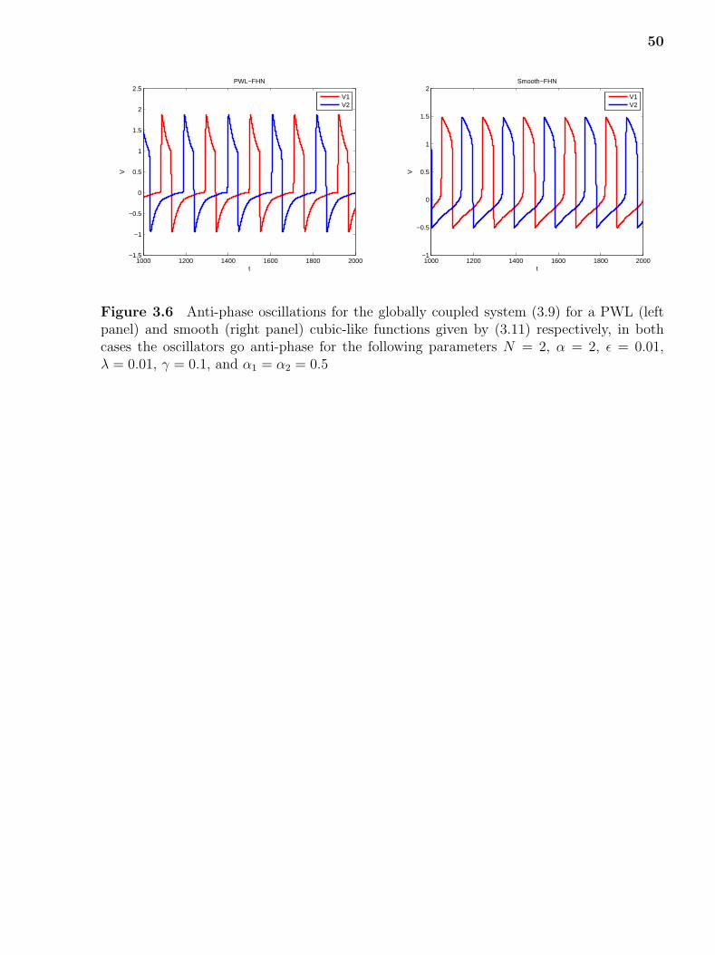
50
1000 1200 1400 1600 1800 2000−1.5
−1
−0.5
0
0.5
1
1.5
2
2.5
t
V
PWL−FHN
V1V2
1000 1200 1400 1600 1800 2000−1
−0.5
0
0.5
1
1.5
2
t
V
Smooth−FHN
V1V2
Figure 3.6 Anti-phase oscillations for the globally coupled system (3.9) for a PWL (leftpanel) and smooth (right panel) cubic-like functions given by (3.11) respectively, in bothcases the oscillators go anti-phase for the following parameters N = 2, α = 2, ε = 0.01,λ = 0.01, γ = 0.1, and α1 = α2 = 0.5

51
1000 1200 1400 1600 1800 2000−1.5
−1
−0.5
0
0.5
1
1.5
2
2.5
t
V(t
)
PWL−FHN
V1V2
1000 1200 1400 1600 1800 2000−1.5
−1
−0.5
0
0.5
1
1.5
2
2.5
t
V(t
)
Smooth−FHN
V1V2
Figure 3.7 Out of phase oscillations for the globally coupled system (3.9) for a PWL (leftpanel) and smooth (right panel) cubic-like functions given by (3.11) respectively, and for thefollowing parameters N = 2, α = 2, ε = 0.01, λ = 0.01, γ = 0.1, and α1 = 0.8, α2 = 0.2
1000 1200 1400 1600 1800 2000−1.5
−1
−0.5
0
0.5
1
1.5
2
2.5
t
V
PWL−FHN
V1V2
1000 1200 1400 1600 1800 2000−1
−0.5
0
0.5
1
1.5
2
t
V
Smooth−FHN
V1V2
Figure 3.8 Anti-phase oscillations for the globally coupled system (3.9) for a PWL (leftpanel) and smooth (right panel) cubic-like functions given by (3.11) respectively, and for thefollowing parameters N = 2, α = 4, ε = 0.01, λ = 0.01, γ = 0.1, and α1 = α2 = 0.5

52
1000 1200 1400 1600 1800 2000−1.5
−1
−0.5
0
0.5
1
1.5
2
2.5
t
VPWL−FHN
V1V2
1000 1200 1400 1600 1800 2000−1
−0.5
0
0.5
1
1.5
2
t
V
Smooth−FHN
V1V2
Figure 3.9 Anti-phase oscillations for the globally coupled system (3.9) for a PWL (leftpanel) and smooth (right panel) cubic-like functions given by (3.11) respectively, and for thefollowing parameters N = 2, α = 4, ε = 0.01, λ = 0.1, γ = 0.1, and α1 = α2 = 0.5
1000 1100 1200 1300 1400 1500−1.5
−1
−0.5
0
0.5
1
1.5
2
2.5
t
V
PWL−FHN
V1V2
0 100 200 300 400 500−0.5
−0.4
−0.3
−0.2
−0.1
0
0.1
0.2
0.3
0.4
0.5
t
V
Smooth−FHN
V1V2
Figure 3.10 Different dynamic behavior between the PWL (left panel) and smooth (rightpanel) globally coupled system (3.11). The cubic like functions are given by (3.9)respectively,and for the following parameters N = 2, α = 4, ε = 0.1, λ = 0.01, γ = 0.1, and α1 =α2 = 0.5. The smooth system exhibits oscillation death while the PWL system exhibitspersistent oscillations. In the PWL system, the ”red” oscillator displays only large amplitudeoscillations while the ”blue” one displays both small amplitude oscillations interspersed withlarge amplitude oscillations (mixed-mode oscillations).

53
0 50 100 150 200−1.5
−1
−0.5
0
0.5
1
1.5
2
2.5
t
V
PWL−FHN
V1V2
0 50 100 150 200−0.5
−0.4
−0.3
−0.2
−0.1
0
0.1
0.2
0.3
0.4
0.5
t
V
Smooth−FHN
V1V2
Figure 3.11 Oscillation death for the globally coupled system (3.11) for a PWL (left panel)and smooth (right panel) cubic-like functions given by (3.9) and (number) respectively, andfor the following parameters N = 2, α = 4, ε = 0.5, λ = 0.01, γ = 0.1, and α1 = α2 = 0.5.
1000 1200 1400 1600 1800 2000−1.5
−1
−0.5
0
0.5
1
1.5
2
2.5
t
V
PWL−FHN
V1V2
1000 1200 1400 1600 1800 2000−1
−0.5
0
0.5
1
1.5
2
t
V
Smooth−FHN
V1V2
Figure 3.12 Out of phase (phase locked) oscillators for the globally coupled systems (3.11)between the PWL(left panel) and smooth (right panel) : N = 2, γ = 0.1, λ = 0.01, ε =0.01, α = 4, α1 = 0.6, α2 = 0.4. The phase of cubic case is 0.5208, the phase of piecewise-linear is 0.5852.

54
1000 1200 1400 1600 1800 2000−1.5
−1
−0.5
0
0.5
1
1.5
2
2.5
t
V
PWL−FHN
V1V2
1000 1200 1400 1600 1800 2000−1
−0.5
0
0.5
1
1.5
2
t
V
Smooth−FHN
V1V2
Figure 3.13 Out of phase (phase locked) oscillators for the FHN model (3.11) between thePWL(left panel) and smooth (right panel) : N = 2, γ = 0.1, λ = 0.01, ε = 0.01, α = 4, α1 =0.7, α2 = 0.3. The phase of cubic case is 0.5407, the phase of piecewise-linear is 0.6252.
1000 1200 1400 1600 1800 2000−1.5
−1
−0.5
0
0.5
1
1.5
2
2.5
t
V
PWL−FHN
V1V2
1000 1200 1400 1600 1800 2000−1
−0.5
0
0.5
1
1.5
2
t
V
Smooth−FHN
V1V2
Figure 3.14 Out of phase (phase locked) oscillators for FHN model (3.11) between thePWL(left panel) and smooth (right panel) : N = 2, γ = 0.1, λ = 0.01, ε = 0.01, α = 4, α1 =0.8, α2 = 0.2. The phase of cubic case is 0.5579, the phase of piecewise-linear is 0.6504.
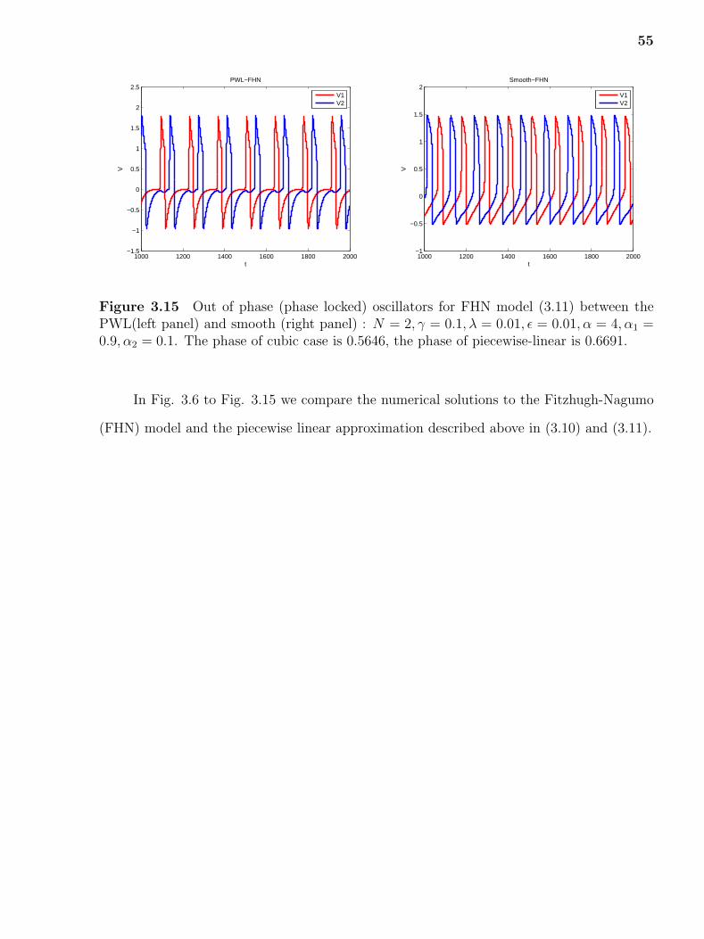
55
1000 1200 1400 1600 1800 2000−1.5
−1
−0.5
0
0.5
1
1.5
2
2.5
t
V
PWL−FHN
V1V2
1000 1200 1400 1600 1800 2000−1
−0.5
0
0.5
1
1.5
2
t
V
Smooth−FHN
V1V2
Figure 3.15 Out of phase (phase locked) oscillators for FHN model (3.11) between thePWL(left panel) and smooth (right panel) : N = 2, γ = 0.1, λ = 0.01, ε = 0.01, α = 4, α1 =0.9, α2 = 0.1. The phase of cubic case is 0.5646, the phase of piecewise-linear is 0.6691.
In Fig. 3.6 to Fig. 3.15 we compare the numerical solutions to the Fitzhugh-Nagumo
(FHN) model and the piecewise linear approximation described above in (3.10) and (3.11).
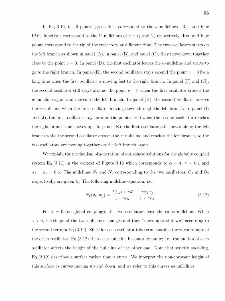
56
In Fig 3.16, in all panels, green lines correspond to the w-nullclines. Red and blue
PWL functions correspond to the V -nullclines of the V1 and V2 respectively. Red and blue
points correspond to the tip of the trajectory at different time. The two oscillators starts on
the left branch as shown in panel (A), in panel (B), and panel (C), they move down together
close to the point v = 0. In panel (D), the first oscillator leaves the w-nullcline and starts to
go to the right branch. In panel (E), the second oscillator stays around the point v = 0 for a
long time when the first oscillator is moving fast to the right branch. In panel (F) and (G),
the second oscillator still stays around the point v = 0 when the first oscillator crosses the
w-nullcline again and moves to the left branch. In panel (H), the second oscillator crosses
the w-nullcline when the first oscillator moving down through the left branch. In panel (I)
and (J), the first oscillator stays around the point v = 0 when the second oscillator reaches
the right branch and moves up. In panel (K), the first oscillator still moves along the left
branch while the second oscillator crosses the w-nullcline and reaches the left branch, so the
two oscillators are moving together on the left branch again.
We explain the mechanism of generation of anti-phase solutions for the globally coupled
system Eq.(3.11) in the context of Figure 3.16 which corresponds to α = 4, γ = 0.1 and
α1 = α2 = 0.5. The nullclines N1 and N2 corresponding to the two oscillators, O1 and O2
respectively, are given by The following nullcline equation; i.e.,
Nk(vk, wj) =f(vk) + γw
1 + γαk
− γαjwj
1 + γαk
(3.12)
For γ = 0 (no global coupling), the two oscillators have the same nullcline. When
γ > 0, the shape of the two nullclines changes and they ”move up and down” according to
the second term in Eq.(3.12). Since for each oscillator this term contains the w-coordinate of
the other oscillator, Eq.(3.12) then each nullcline becomes dynamic; i.e., the motion of each
oscillator affects the height of the nullcline of the other one. Note that strictly speaking,
Eq.(3.12) describes a surface rather than a curve. We interpret the non-constant height of
this surface as curves moving up and down, and we refer to this curves as nullclines.

57
A B
−1 −0.5 0 0.5 1 1.5 2−0.2
0
0.2
0.4
0.6
0.8
1
1.2
1.4
V
Wt=0
w nullclinev1 nullclinev2 nullclineoscillator 1oscillator 2
−1 −0.5 0 0.5 1 1.5 2−0.2
0
0.2
0.4
0.6
0.8
1
1.2
1.4
t=25
V
W
C Cz
−1 −0.5 0 0.5 1 1.5 2−0.2
0
0.2
0.4
0.6
0.8
1
1.2
1.4
t=96
V
W
−6 −4 −2 0 2 4 6
x 10−3
−0.5
0
0.5
1
1.5
2
2.5
3
3.5
4x 10
−3 t=96
V
W
D Dz
−1 −0.5 0 0.5 1 1.5 2−0.2
0
0.2
0.4
0.6
0.8
1
1.2
1.4
t=102
V
W
−5 0 5 10 15
x 10−3
−0.5
0
0.5
1
1.5
2
2.5
3
3.5
4x 10
−3 t=102
V
W

58
E Ez
−1 −0.5 0 0.5 1 1.5 2−0.2
0
0.2
0.4
0.6
0.8
1
1.2
1.4
t=107
V
W
−6 −4 −2 0 2 4 6 8 10
x 10−3
−6
−5
−4
−3
−2
−1
0
1
2
3
4x 10
−3 t=107
V
W
F G
−1 −0.5 0 0.5 1 1.5 2−0.2
0
0.2
0.4
0.6
0.8
1
1.2
1.4
t=114
V
W
−1 −0.5 0 0.5 1 1.5 2−0.2
0
0.2
0.4
0.6
0.8
1
1.2
1.4
t=126
V
W
H I
−1 −0.5 0 0.5 1 1.5 2−0.2
0
0.2
0.4
0.6
0.8
1
1.2
1.4
t=135
V
W
−1 −0.5 0 0.5 1 1.5 2−0.2
0
0.2
0.4
0.6
0.8
1
1.2
1.4
t=150
V
W

59
J K
−1 −0.5 0 0.5 1 1.5 2−0.2
0
0.2
0.4
0.6
0.8
1
1.2
1.4
t=167
V
W
−1 −0.5 0 0.5 1 1.5 2−0.2
0
0.2
0.4
0.6
0.8
1
1.2
1.4
t=174
V
W
Figure 3.16 Two globally coupled oscillators moving with equation (3.11) in piecewise-linear case, and two anti-phase clusters for the following parameters: α = 4, γ = 0.1, α1 =0.5, α2 = 0.5
Fig. 3.16-A shows the initial location of the two oscillators. We set the initial conditions
lying in a vicinity of the left branch of the corresponding nullclines N1 and N2. In Fig. 3.16,
oscillator O1 is marked in red and oscillator O2 is marked in blue. The full dots correspond
to the tip of the trajectory for the time shown in the top of the panel. When appropriate for
the geometric description of the dynamics we will refer to the w-coordinates of the red and
blue oscillators as wr and wb respectively and to the corresponding nullclines as Nr and Nb.
Since ε << 1 the trajectories of the two oscillators will evolve in a vicinity of Nr and
Nb. As time increases the two oscillators move down along these nullclines and get closer
together (the distance between their locations decreases) but the order is preserved; i.e., the
red oscillator is ahead of the blue oscillator as long both are moving along the left branch of
the v-nullclines (Fig. 3.16-B, Fig. 3.16-C and Fig. 3.16-Cz).
The red oscillator arrives to the minimum of Nr before the blue oscillator arrives to
the minimum of Nb. This is due to the fact that wr < wb. When the red oscillators reaches
the minimum of Nr it moves along a fast direction of motion towards the right branch of Nr.
This direction is almost horizontal with a small vertical component. This slight increase in
the value of wr causes Nb to move down (Fig. 3.16-E and Fig. 3.16)-Ez thus preventing the

60
blue oscillator from crossing to the middle branch regime. Once the red oscillator arrives to
a vicinity of the right branch of Nr it moves in moves along it in the upward direction (Fig.
3.16)-F which further prevents the blue oscillator from crossing to the left branch of Nb due
to the increase in the value of wr. Only when the red oscillator returns to a vicinity of the
left branch of Nr moves down along it decreasing value of wr (Fig.3.16-G to Fig. 3.16)-I the
nullcline Nb moves up and allows the blue oscillator to move to the right branch of Nb (Fig.
3.16)-I and move up along it while the red oscillator moves down along Nr (Fig. 3.16)-J.
When the blue oscillator returns to the left branch of Nb the red oscillators is close to the
minimum of Nr. The distance between the their location is larger than initially (Compare
Fig. 3.16-K and Fig. 3.16)-A so the oscillators will never synchronize in phase.
The similar dynamical process is shown in Fig. 3.17 to Fig. 3.19 in both of piecewise
linear case and cubic case.
61
In the figures Fig. 3.20 to Fig. 3.23, α1 6= 0.5 and α2 6= 0.5, so we get out of phase
pattern instead of anti-phase pattern.

62
A B
−1 −0.5 0 0.5 1 1.5 2−0.2
0
0.2
0.4
0.6
0.8
1
1.2
1.4
V
Wt=0
w nullclinev1 nullclinev2 nullclineoscillator 1oscillator 2
−1 −0.5 0 0.5 1 1.5 2−0.2
0
0.2
0.4
0.6
0.8
1
1.2
1.4
t=42
V
W
Bz C
−0.1 −0.08 −0.06 −0.04 −0.02 0 0.02
0
0.005
0.01
0.015
0.02
0.025
0.03t=42
V
W
−1 −0.5 0 0.5 1 1.5 2−0.2
0
0.2
0.4
0.6
0.8
1
1.2
1.4
t=53
V
W
Cz D
−0.1 −0.05 0 0.05 0.1−0.015
−0.01
−0.005
0
0.005
0.01
0.015
0.02
0.025
0.03t=53
V
W
−1 −0.5 0 0.5 1 1.5 2−0.2
0
0.2
0.4
0.6
0.8
1
1.2
1.4
t=62
V
W

63
Dz E
0 0.05 0.1 0.15 0.2 0.25−0.005
0
0.005
0.01
0.015
0.02
0.025
t=62
V
W
−1 −0.5 0 0.5 1 1.5 2−0.2
0
0.2
0.4
0.6
0.8
1
1.2
1.4
t=65
V
W
Ez F
0 0.02 0.04 0.06 0.08 0.1−6
−4
−2
0
2
4
6
8
10
12
14x 10
−3 t=65
V
W
−1 −0.5 0 0.5 1 1.5 2−0.2
0
0.2
0.4
0.6
0.8
1
1.2
1.4
t=69
V
W
G H
−1 −0.5 0 0.5 1 1.5 2−0.2
0
0.2
0.4
0.6
0.8
1
1.2
1.4
t=88
V
W
−1 −0.5 0 0.5 1 1.5 2−0.2
0
0.2
0.4
0.6
0.8
1
1.2
1.4
t=89
V
W

64
I J
−1 −0.5 0 0.5 1 1.5 2−0.2
0
0.2
0.4
0.6
0.8
1
1.2
1.4
t=108
V
W
−1 −0.5 0 0.5 1 1.5 2−0.2
0
0.2
0.4
0.6
0.8
1
1.2
1.4
t=129
V
W
K L
−1 −0.5 0 0.5 1 1.5 2−0.2
0
0.2
0.4
0.6
0.8
1
1.2
1.4
t=131
V
W
−1 −0.5 0 0.5 1 1.5 2−0.2
0
0.2
0.4
0.6
0.8
1
1.2
1.4
t=133.8369
V
W
Figure 3.17 Two globally coupled oscillators moving with equation (3.11) in cubic case,and two anti-phase clusters for the following parameters: α = 4, γ = 0.1, α1 = 0.5, α2 = 0.5

65
A B
−1 −0.5 0 0.5 1 1.5 2−0.2
0
0.2
0.4
0.6
0.8
1
1.2
1.4
V
Wt=0
w nullclinev1 nullclinev2 nullclineoscillator 1oscillator 2
−1 −0.5 0 0.5 1 1.5 2−0.2
0
0.2
0.4
0.6
0.8
1
1.2
1.4
t= 163.1704
V
W
Bz C
−1 −0.5 0 0.5 1 1.5 2−0.2
0
0.2
0.4
0.6
0.8
1
1.2
1.4
t=169.6185
V
W
Cz D
−0.01 −0.005 0 0.005 0.01−2
−1
0
1
2
3
4
5
6
7
8x 10
−3 t=169.6185
V
W
−1 −0.5 0 0.5 1 1.5 2−0.2
0
0.2
0.4
0.6
0.8
1
1.2
1.4
t=182.1384
V
W

66
Dz E
−0.03 −0.025 −0.02 −0.015 −0.01 −0.005 0 0.005−0.025
−0.02
−0.015
−0.01
−0.005
0
0.005
0.01t=182.1384
V
W
−1 −0.5 0 0.5 1 1.5 2−0.2
0
0.2
0.4
0.6
0.8
1
1.2
1.4
t= 216.8834
V
W
F G
−1 −0.5 0 0.5 1 1.5 2−0.2
0
0.2
0.4
0.6
0.8
1
1.2
1.4
t= 220.4876
V
W
−1 −0.5 0 0.5 1 1.5 2−0.2
0
0.2
0.4
0.6
0.8
1
1.2
1.4
t= 240.2171
V
W
H I
−1 −0.5 0 0.5 1 1.5 2−0.2
0
0.2
0.4
0.6
0.8
1
1.2
1.4
t= 247.6789
V
W
−1 −0.5 0 0.5 1 1.5 2−0.2
0
0.2
0.4
0.6
0.8
1
1.2
1.4
t= 265.4784
V
W

67
J
−1 −0.5 0 0.5 1 1.5 2−0.2
0
0.2
0.4
0.6
0.8
1
1.2
1.4
t= 303.1279
V
W
Figure 3.18 Two globally coupled oscillators moving with equation (3.11) in piecewise-linear case, and two anti-phase clusters for the following parameters: α = 2, γ = 0.1, α1 =0.5, α2 = 0.5
In Fig. 3.20 to Fig. 3.23, the oscillators go out of-phase instead of anti-phase in both
of cubic oscillators and the piecewise linear approximated oscillators, but the dynamical
process is the same as Fig. 3.16 to Fig. 3.19.
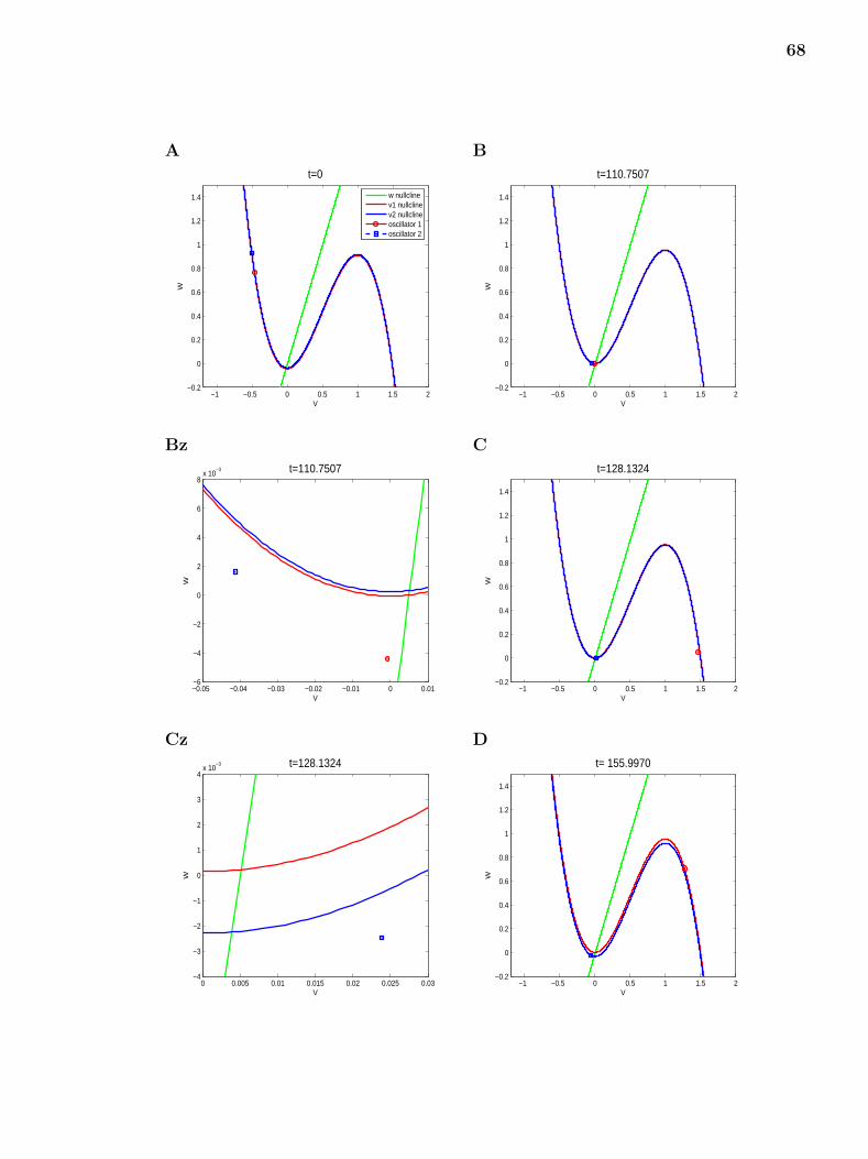
68
A B
−1 −0.5 0 0.5 1 1.5 2−0.2
0
0.2
0.4
0.6
0.8
1
1.2
1.4
V
Wt=0
w nullclinev1 nullclinev2 nullclineoscillator 1oscillator 2
−1 −0.5 0 0.5 1 1.5 2−0.2
0
0.2
0.4
0.6
0.8
1
1.2
1.4
t=110.7507
V
W
Bz C
−0.05 −0.04 −0.03 −0.02 −0.01 0 0.01−6
−4
−2
0
2
4
6
8x 10
−3 t=110.7507
V
W
−1 −0.5 0 0.5 1 1.5 2−0.2
0
0.2
0.4
0.6
0.8
1
1.2
1.4
t=128.1324
V
W
Cz D
0 0.005 0.01 0.015 0.02 0.025 0.03−4
−3
−2
−1
0
1
2
3
4x 10
−3 t=128.1324
V
W
−1 −0.5 0 0.5 1 1.5 2−0.2
0
0.2
0.4
0.6
0.8
1
1.2
1.4
t= 155.9970
V
W

69
E F
−1 −0.5 0 0.5 1 1.5 2−0.2
0
0.2
0.4
0.6
0.8
1
1.2
1.4
t= 179.0829
V
W
−1 −0.5 0 0.5 1 1.5 2−0.2
0
0.2
0.4
0.6
0.8
1
1.2
1.4
t= 180.6890
V
W
G H
−1 −0.5 0 0.5 1 1.5 2−0.2
0
0.2
0.4
0.6
0.8
1
1.2
1.4
t= 196.4557
V
W
−1 −0.5 0 0.5 1 1.5 2−0.2
0
0.2
0.4
0.6
0.8
1
1.2
1.4
t= 202.3325
V
W
I J
−1 −0.5 0 0.5 1 1.5 2−0.2
0
0.2
0.4
0.6
0.8
1
1.2
1.4
t= 244.5539
V
W
−1 −0.5 0 0.5 1 1.5 2−0.2
0
0.2
0.4
0.6
0.8
1
1.2
1.4
t= 254.9048
V
W
Figure 3.19 Two globally coupled oscillators moving with equation (3.11) in cubic case,and two anti-phase clusters for the following parameters: α = 2, γ = 0.1, α1 = 0.5, α2 = 0.5

70
A B
−1 −0.5 0 0.5 1 1.5 2−0.2
0
0.2
0.4
0.6
0.8
1
1.2
1.4
V
Wt=0
w nullclinev1 nullclinev2 nullclineoscillator 1oscillator 2
−1 −0.5 0 0.5 1 1.5 2−0.2
0
0.2
0.4
0.6
0.8
1
1.2
1.4
t=163.8751
V
W
Bz C
−15 −10 −5 0 5
x 10−3
−2
0
2
4
6
8
10x 10
−3 t=163.8751
V
W
−1 −0.5 0 0.5 1 1.5 2−0.2
0
0.2
0.4
0.6
0.8
1
1.2
1.4
t=170.9164
V
W
Cz D
−15 −10 −5 0 5
x 10−3
−2
0
2
4
6
8
10x 10
−3 t=170.9164
V
W
−1 −0.5 0 0.5 1 1.5 2−0.2
0
0.2
0.4
0.6
0.8
1
1.2
1.4
t=178.3717
V
W

71
Dz E
−15 −10 −5 0 5
x 10−3
−0.01
−0.008
−0.006
−0.004
−0.002
0
0.002
0.004
0.006
0.008
0.01t=178.3717
−1 −0.5 0 0.5 1 1.5 2−0.2
0
0.2
0.4
0.6
0.8
1
1.2
1.4
t= 196.0158
V
W
Ez F
−10 −5 0 5
x 10−3
−0.025
−0.02
−0.015
−0.01
−0.005
0t= 196.0158
−1 −0.5 0 0.5 1 1.5 2−0.2
0
0.2
0.4
0.6
0.8
1
1.2
1.4
t= 225.2868
V
W
G H
−1 −0.5 0 0.5 1 1.5 2−0.2
0
0.2
0.4
0.6
0.8
1
1.2
1.4
t= 257.7769
V
W
−1 −0.5 0 0.5 1 1.5 2−0.2
0
0.2
0.4
0.6
0.8
1
1.2
1.4
t= 349.1520
V
W

72
I J
−1 −0.5 0 0.5 1 1.5 2−0.2
0
0.2
0.4
0.6
0.8
1
1.2
1.4
t= 356.7315
V
W
−1 −0.5 0 0.5 1 1.5 2−0.2
0
0.2
0.4
0.6
0.8
1
1.2
1.4
t= 367.8037
V
W
Figure 3.20 Two globally coupled oscillators moving with equation (3.11) in piecewise-linear case, and two out of phase clusters for the following parameters: α = 4, γ = 0.1, α1 =0.8, α2 = 0.2
3.4 Solution of Piecewise Linear Oscillators
The equations of two globally coupled piecewise oscillators can be expand as:
v′1 = a(v1 − v0)− ω1 − γ(α1ω1 + α2ω2 − ω)
v′2 = b(v2 − v0)− ω2 − γ(α1ω1 + α2ω2 − ω)
ω′1 = ε(αv1 − λ− ω1)
ω′2 = ε(αv2 − λ− ω2)
(3.13)
Where parameter a, v0 are determined by the position or the branch of the first
oscillator, b, v0 are determined by the position or the branch of the second oscillator.
The above equation (3.13) can be written to a matrix form:
v1′
v2′
ω1′
ω2′
=
a 0 −(1 + γα1) −γα2
0 b −γα1 −(1 + γα2)
εα 0 −ε 0
0 εα 0 −ε
v1
v2
ω1
ω2
+
−av0 + γω
−bv0 + γω
−ελ
−ελ
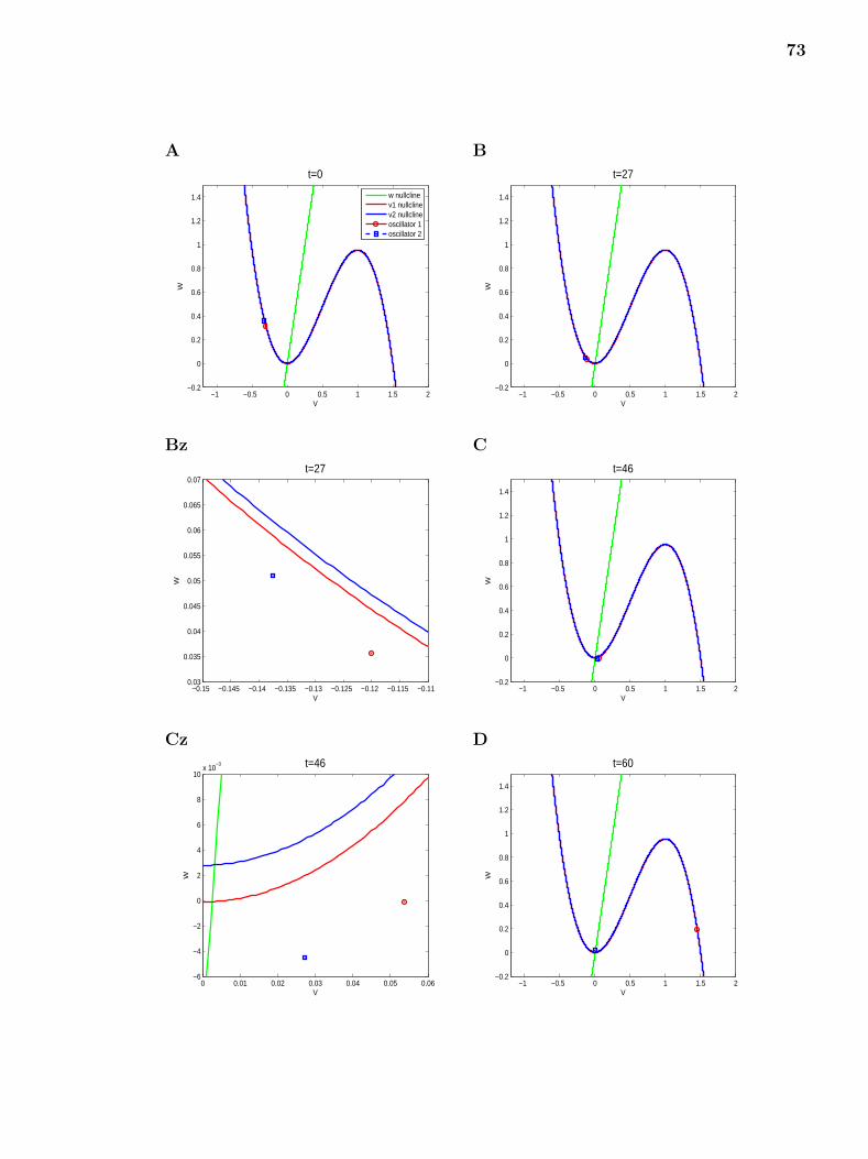
73
A B
−1 −0.5 0 0.5 1 1.5 2−0.2
0
0.2
0.4
0.6
0.8
1
1.2
1.4
V
Wt=0
w nullclinev1 nullclinev2 nullclineoscillator 1oscillator 2
−1 −0.5 0 0.5 1 1.5 2−0.2
0
0.2
0.4
0.6
0.8
1
1.2
1.4
t=27
V
W
Bz C
−0.15 −0.145 −0.14 −0.135 −0.13 −0.125 −0.12 −0.115 −0.110.03
0.035
0.04
0.045
0.05
0.055
0.06
0.065
0.07t=27
V
W
−1 −0.5 0 0.5 1 1.5 2−0.2
0
0.2
0.4
0.6
0.8
1
1.2
1.4
t=46
V
W
Cz D
0 0.01 0.02 0.03 0.04 0.05 0.06−6
−4
−2
0
2
4
6
8
10x 10
−3 t=46
V
W
−1 −0.5 0 0.5 1 1.5 2−0.2
0
0.2
0.4
0.6
0.8
1
1.2
1.4
t=60
V
W

74
Dz E
−0.06 −0.04 −0.02 0 0.02 0.04 0.06
0
0.005
0.01
0.015
0.02
0.025t=60
V
W
−1 −0.5 0 0.5 1 1.5 2−0.2
0
0.2
0.4
0.6
0.8
1
1.2
1.4
t=72
V
W
F G
−1 −0.5 0 0.5 1 1.5 2−0.2
0
0.2
0.4
0.6
0.8
1
1.2
1.4
t=83
V
W
−1 −0.5 0 0.5 1 1.5 2−0.2
0
0.2
0.4
0.6
0.8
1
1.2
1.4
t=86
V
W
H I
−1 −0.5 0 0.5 1 1.5 2−0.2
0
0.2
0.4
0.6
0.8
1
1.2
1.4
t=102
V
W
−1 −0.5 0 0.5 1 1.5 2−0.2
0
0.2
0.4
0.6
0.8
1
1.2
1.4
t=123
V
W

75
J
−1 −0.5 0 0.5 1 1.5 2−0.2
0
0.2
0.4
0.6
0.8
1
1.2
1.4
t=125
V
W
Figure 3.21 Two globally coupled oscillators moving with equation (3.11), and two out ofphase clusters for the following parameters:α = 4, γ = 0.1, α1 = 0.8, α2 = 0.2
Theorem 1 Consider a four variable ODE system given as follows:
v1′
v2′
ω1′
ω2′
= D
v1
v2
ω1
ω2
+ L
The matrix D can be diagonalized:
D =
a 0 −(1 + γα1) −γα2
0 b −γα1 −(1 + γα2)
εα 0 −ε 0
0 εα 0 −ε
= A
λ1 0 0 0
0 λ2 0 0
0 0 λ3 0
0 0 0 λ4
A−1
where A is a matrix whose columns are eigenvectors of D.
The solution of this ODE system is:

76
A B
−1 −0.5 0 0.5 1 1.5 2−0.2
0
0.2
0.4
0.6
0.8
1
1.2
1.4
V
Wt=0
w nullclinev1 nullclinev2 nullclineoscillator 1oscillator 2
−1 −0.5 0 0.5 1 1.5 2−0.2
0
0.2
0.4
0.6
0.8
1
1.2
1.4
t=55.5374
V
W
C Cz
−1 −0.5 0 0.5 1 1.5 2−0.2
0
0.2
0.4
0.6
0.8
1
1.2
1.4
t=163.5202
V
W
−0.02 −0.015 −0.01 −0.005 0 0.005 0.01 0.015 0.02
0
0.005
0.01
0.015
0.02
0.025t=163.5202
V
W
D Dz
−1 −0.5 0 0.5 1 1.5 2−0.2
0
0.2
0.4
0.6
0.8
1
1.2
1.4
t= 170.3128
V
W
−0.02 −0.015 −0.01 −0.005 0 0.005 0.01 0.015 0.02
0
0.005
0.01
0.015
0.02
0.025t= 170.3128
V
W
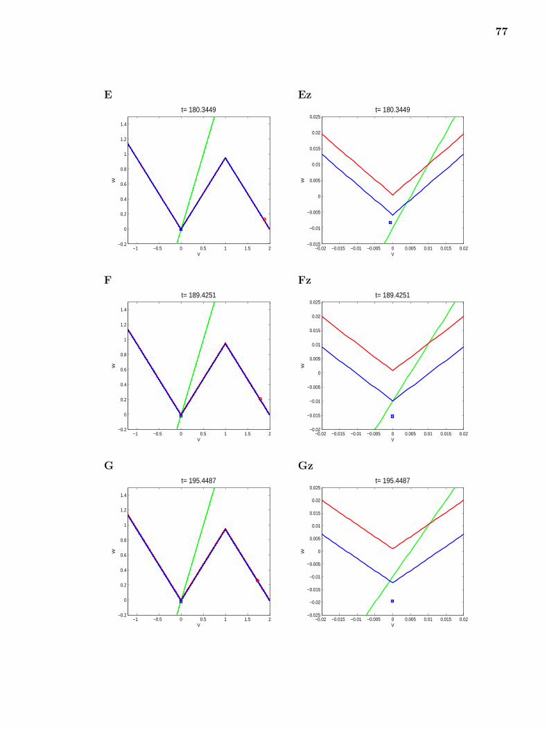
77
E Ez
−1 −0.5 0 0.5 1 1.5 2−0.2
0
0.2
0.4
0.6
0.8
1
1.2
1.4
t= 180.3449
V
W
−0.02 −0.015 −0.01 −0.005 0 0.005 0.01 0.015 0.02−0.015
−0.01
−0.005
0
0.005
0.01
0.015
0.02
0.025t= 180.3449
V
W
F Fz
−1 −0.5 0 0.5 1 1.5 2−0.2
0
0.2
0.4
0.6
0.8
1
1.2
1.4
t= 189.4251
V
W
−0.02 −0.015 −0.01 −0.005 0 0.005 0.01 0.015 0.02−0.02
−0.015
−0.01
−0.005
0
0.005
0.01
0.015
0.02
0.025t= 189.4251
V
W
G Gz
−1 −0.5 0 0.5 1 1.5 2−0.2
0
0.2
0.4
0.6
0.8
1
1.2
1.4
t= 195.4487
V
W
−0.02 −0.015 −0.01 −0.005 0 0.005 0.01 0.015 0.02−0.025
−0.02
−0.015
−0.01
−0.005
0
0.005
0.01
0.015
0.02
0.025t= 195.4487
V
W

78
H Hz
−1 −0.5 0 0.5 1 1.5 2−0.2
0
0.2
0.4
0.6
0.8
1
1.2
1.4
t= 203.9981
V
W
−0.02 −0.015 −0.01 −0.005 0 0.005 0.01 0.015 0.02−0.03
−0.025
−0.02
−0.015
−0.01
−0.005
0
0.005
0.01
0.015
0.02
t= 203.9981
V
W
I Iz
−1 −0.5 0 0.5 1 1.5 2−0.2
0
0.2
0.4
0.6
0.8
1
1.2
1.4
t= 212.1995
V
W
−0.02 −0.015 −0.01 −0.005 0 0.005 0.01 0.015 0.02
−0.03
−0.02
−0.01
0
0.01
0.02
t= 212.1995
V
W
J Jz
−1 −0.5 0 0.5 1 1.5 2−0.2
0
0.2
0.4
0.6
0.8
1
1.2
1.4
t= 336.6038
V
W
−0.02 −0.015 −0.01 −0.005 0 0.005 0.01 0.015 0.02−0.08
−0.07
−0.06
−0.05
−0.04
−0.03
−0.02
−0.01
0
0.01
0.02
t= 336.6038
V
W

79
K
−1 −0.5 0 0.5 1 1.5 2−0.2
0
0.2
0.4
0.6
0.8
1
1.2
1.4
t= 619.9635
V
W
Figure 3.22 Two globally coupled oscillators moving with equation (3.11) in piecewise-linear case, and two out of phase clusters for the following parameters: α = 2, γ = 0.1, α1 =0.8, α2 = 0.2
v1
v2
ω1
ω2
= A
1λ1
0 0 0
0 1λ2
0 0
0 0 1λ3
0
0 0 0 1λ4
·
eλ1t 0 0 0
0 eλ2t 0 0
0 0 eλ3t 0
0 0 0 eλ4t
λ1 0 0 0
0 λ2 0 0
0 0 λ3 0
0 0 0 λ4
A−1
v1(0)
v2(0)
ω1(0)
ω2(0)
+ A−1L
− A−1L
(3.14)
The sketch of the proof is given in Appendix (A.1).
The value of matrix D and vector L is determined by the position of the oscillators,
so we consider nine cases:
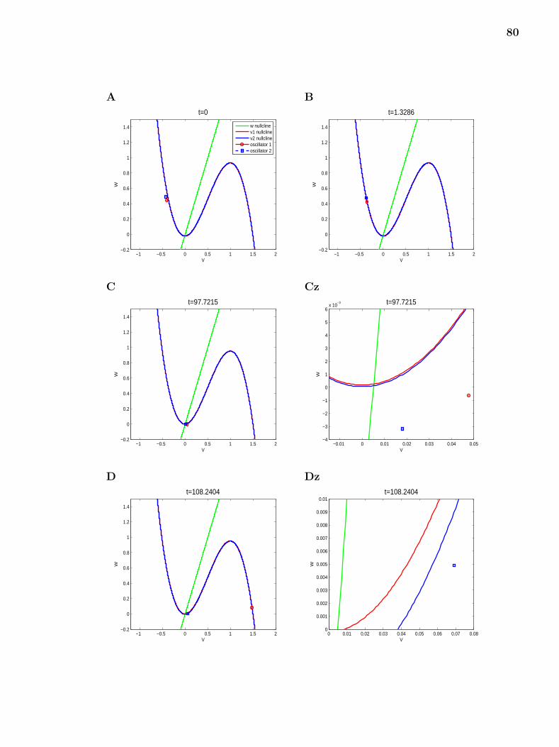
80
A B
−1 −0.5 0 0.5 1 1.5 2−0.2
0
0.2
0.4
0.6
0.8
1
1.2
1.4
V
Wt=0
w nullclinev1 nullclinev2 nullclineoscillator 1oscillator 2
−1 −0.5 0 0.5 1 1.5 2−0.2
0
0.2
0.4
0.6
0.8
1
1.2
1.4
t=1.3286
V
W
C Cz
−1 −0.5 0 0.5 1 1.5 2−0.2
0
0.2
0.4
0.6
0.8
1
1.2
1.4
t=97.7215
V
W
−0.01 0 0.01 0.02 0.03 0.04 0.05−4
−3
−2
−1
0
1
2
3
4
5
6x 10
−3 t=97.7215
V
W
D Dz
−1 −0.5 0 0.5 1 1.5 2−0.2
0
0.2
0.4
0.6
0.8
1
1.2
1.4
t=108.2404
V
W
0 0.01 0.02 0.03 0.04 0.05 0.06 0.07 0.080
0.001
0.002
0.003
0.004
0.005
0.006
0.007
0.008
0.009
0.01t=108.2404
V
W

81
E Ez
−1 −0.5 0 0.5 1 1.5 2−0.2
0
0.2
0.4
0.6
0.8
1
1.2
1.4
t=118.1280
V
W
−0.1 −0.09 −0.08 −0.07 −0.06 −0.05−5
0
5
10
15
20x 10
−3 t=118.1280
V
W
F G
−1 −0.5 0 0.5 1 1.5 2−0.2
0
0.2
0.4
0.6
0.8
1
1.2
1.4
t= 152.2658
V
W
−1 −0.5 0 0.5 1 1.5 2−0.2
0
0.2
0.4
0.6
0.8
1
1.2
1.4
t= 156.5928
V
W
H I
−1 −0.5 0 0.5 1 1.5 2−0.2
0
0.2
0.4
0.6
0.8
1
1.2
1.4
t= 159.6346
V
W
−1 −0.5 0 0.5 1 1.5 2−0.2
0
0.2
0.4
0.6
0.8
1
1.2
1.4
t= 176.8620
V
W

82
J
−1 −0.5 0 0.5 1 1.5 2−0.2
0
0.2
0.4
0.6
0.8
1
1.2
1.4
t= 182.0241
V
W
Figure 3.23 Two globally coupled oscillators moving with equation (3.11), and two out ofphase clusters for the following parameters:α = 2, γ = 0.1, α1 = 0.8, α2 = 0.2
(i) If both of v1, v2 are moving on the left branch, a = b = −β1,
D =
−β1 0 −(1 + γα1) −γα2
0 −β1 −γα1 −(1 + γα2)
εα 0 −ε 0
0 εα 0 −ε
L =
γω
γω
−ελ
−ελ
(ii) v1 is moving on the left branch, v2 is moving on the middle branch: a =
−β1, b = 1,
D =
−β1 0 −(1 + γα1) −γα2
0 1 −γα1 −(1 + γα2)
εα 0 −ε 0
0 εα 0 −ε
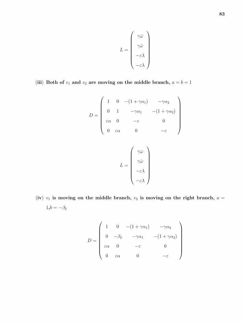
83
L =
γω
γω
−ελ
−ελ
(iii) Both of v1 and v2 are moving on the middle branch, a = b = 1
D =
1 0 −(1 + γα1) −γα2
0 1 −γα1 −(1 + γα2)
εα 0 −ε 0
0 εα 0 −ε
L =
γω
γω
−ελ
−ελ
(iv) v1 is moving on the middle branch, v2 is moving on the right branch, a =
1,b = −β2
D =
1 0 −(1 + γα1) −γα2
0 −β2 −γα1 −(1 + γα2)
εα 0 −ε 0
0 εα 0 −ε

84
L =
γω
γω + 1 + β2
−ελ
−ελ
(v) Both of v1 and v2 are moving on the right branch, a = b = −β2
D =
−β2 0 −(1 + γα1) −γα2
0 −β2 −γα1 −(1 + γα2)
εα 0 −ε 0
0 εα 0 −ε
L =
γω + 1 + β2
γω + 1 + β2
−ελ
−ελ
(vi) v2 is moving on the middle branch, v1 is moving on the right branch, a = −β2,
b = 1
D =
−β2 0 −(1 + γα1) −γα2
0 1 −γα1 −(1 + γα2)
εα 0 −ε 0
0 εα 0 −ε

85
L =
γω + 1 + β2
γω
−ελ
−ελ
(vii) v2 is moving on the left branch, v1 is moving on the middle branch, a = 1,
b = −β1
D =
1 0 −(1 + γα1) −γα2
0 −β1 −γα1 −(1 + γα2)
εα 0 −ε 0
0 εα 0 −ε
L =
γω
γω
−ελ
−ελ
(viii) v1 is moving on the left branch, v2 is moving on the right branch, a = −β1,
b = −β2
D =
−β1 0 −(1 + γα1) −γα2
0 −β2 −γα1 −(1 + γα2)
εα 0 −ε 0
0 εα 0 −ε

86
L =
γω
γω + 1 + β2
−ελ
−ελ
(ix) v2 is moving on the right branch, v1 is moving on the left branch, a = −β1,
b = −β2
D =
−β2 0 −(1 + γα1) −γα2
0 −β1 −γα1 −(1 + γα2)
εα 0 −ε 0
0 εα 0 −ε
L =
γω + 1 + β2
γω
−ελ
−ελ
This is the exact solution of v1(t), v2(t), ω1(t), ω2(t). To see whether two oscillators
can synchronize after a long time, we need to see whether limt→∞ v1(t)− v2(t) = 0.
3.5 Comparison of Analytical Solution and Numerical Solution for Two
Piecewise Linear Coupling Oscillators
We use piecewise linear system to approximate cubic system, so we want to check the patterns
of piecewise linear coupling oscillators. The analytical solution for two piecewise linear
coupling oscillators is given in equation (3.14).
In order to check if numerical simulations accurately predicts the analytical solutions
of the oscillators, an important step is to check the error of the numerical simulation.

87
The equations of dynamical system with global coupling terms are given in (3.10) and
(3.11). We fix the coefficients and the initial conditions as follows:
The graph is shown in Fig. 3.24. The analytical solution is given by the (3.14) above.
The error of functions v(t) and ω(t) between the numerical (2-stage-Runge-Kutta(RK2)
scheme [5, 6] and the analytical solutions is very small. So the numerical simulation makes
accurate prediction for the phase property of the analytical solutions. If the numerical
solutions of two oscillators go anti-phase(same phase), the exact solutions will also go anti-
phase(same phase).
3.6 The Moving Nullclines Approach
Lemma of moving nullclines
Lemma 3.6.1 For the two piecewise linear oscillators system (3.10),(3.11), the nullcline of
one oscillator (vk, ωk) is moving up(moving down) ⇔ The other oscillator (vi, ωi) lies on the
left side (right side) of ω nullcline.
The sketch of the proof is given in the appendix (A.2).
The moving nullclines graphs are shown in Fig 3.25.
The function of global feedback oscillators is:
v′k = f(vk)− ωk − 0.2 · (12ωk + 1
2ωi − ω)
ω′k = 0.01(10vk − 0.2− ωk)(3.15)
where
f(v) =
−v, when v < 0
v, when 0 ≤ v ≤ 1
2− v, when v > 1
(3.16)
When both of the initial points are on the left branch, both oscillators lie on the
left side of the ω- nullcline, ω′j = αvj − λ − ωj < 0, both v-nullclines move up in the

88
A
0 200 400 600 800 1000−1
−0.5
0
0.5
1
1.5
2
t
V1
numberical solution of v1
exact solution of v1
0 200 400 600 800 10000
0.02
0.04
0.06
0.08
0.1
t
Err
or
of V
1
0 200 400 600 800 1000−0.2
0
0.2
0.4
0.6
0.8
1
1.2
t
W1
numberical solution of w1
exact solution of w1
0 200 400 600 800 10000
1
2
3
4
5x 10
−3
t
Err
or
of
W1
0 200 400 600 800 1000−1
−0.5
0
0.5
1
1.5
2
t
V2
numberical solution of v
2
exact solution of v2
0 200 400 600 800 10000
0.01
0.02
0.03
0.04
0.05
0.06
0.07
t
Err
or
of V
2

89
0 200 400 600 800 1000−0.2
0
0.2
0.4
0.6
0.8
1
1.2
t
W2
numberical solution of w2
exact solution of w2
0 200 400 600 800 10000
0.5
1
1.5
2x 10
−3
t
Err
or
of
W2
B
0 200 400 600 800 1000−1
−0.5
0
0.5
1
1.5
2
t
V1
numberical solution of v1
exact solution of v1
0 200 400 600 800 10000
0.02
0.04
0.06
0.08
0.1
t
Err
or
of V
1
0 200 400 600 800 1000−0.2
0
0.2
0.4
0.6
0.8
1
1.2
t
W1
numberical solution of w1
exact solution of w1
0 200 400 600 800 10000
1
2
3
4
5
6
7
8x 10
−3
t
Err
or
of
W1

90
0 200 400 600 800 1000−1
−0.5
0
0.5
1
1.5
2
t
V2
numberical solution of v2
exact solution of v2
0 200 400 600 800 10000
0.02
0.04
0.06
0.08
0.1
t
Err
or
of V
2
0 200 400 600 800 1000−0.2
0
0.2
0.4
0.6
0.8
1
1.2
t
W2
numberical solution of w
2
exact solution of w2
0 200 400 600 800 10000
1
2
3
4
5
6
7
8x 10
−3
t
Err
or
of
W2
C
0 200 400 600 800 1000−1
−0.5
0
0.5
1
1.5
2
t
V1
numberical solution of v1
exact solution of v1
0 200 400 600 800 10000
0.02
0.04
0.06
0.08
0.1
t
Err
or
of V
1

91
0 200 400 600 800 1000−0.2
0
0.2
0.4
0.6
0.8
1
1.2
t
W1
numberical solution of w
1
exact solution of w1
0 200 400 600 800 10000
0.002
0.004
0.006
0.008
0.01
t
Err
or
of W
1
0 200 400 600 800 1000−1
−0.5
0
0.5
1
1.5
2
t
V2
numberical solution of v
2
exact solution of v2
0 200 400 600 800 10000
0.02
0.04
0.06
0.08
0.1
t
Err
or
of V
2
0 200 400 600 800 1000−0.2
0
0.2
0.4
0.6
0.8
1
1.2
t
W2
numberical solution of w2
exact solution of w2
0 200 400 600 800 10000
1
2
3
4
5
6
7
8x 10
−3
t
Err
or
of
W2
Figure 3.24 Comparison of the numerical solution and exact solution of two oscillatorssystem by initial conditions:v1(0) = −1, ω1(0) = 0.5, v2(0) = −0.65, ω2(0) = 0.35 Thereare three set of parameters: (A) λ = 0.2, (B) λ = 0.1 and (C) λ = 0.01; other parametersγ = 0.1, ε = 0.01, α = 2, β1 = 1, β2 = 1
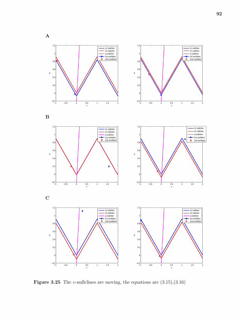
92
A
−1 −0.5 0 0.5 1 1.5 2−0.2
0
0.2
0.4
0.6
0.8
1
1.2
v
ω
v1 nullclinev2 nullclineω nullcline1st oscillator2nd oscillator
−1 −0.5 0 0.5 1 1.5 2−0.2
0
0.2
0.4
0.6
0.8
1
1.2
v
ω
v1 nullclinev2 nullclineω nullcline1st oscillator2nd oscillator
B
−1 −0.5 0 0.5 1 1.5 2−0.2
0
0.2
0.4
0.6
0.8
1
1.2
v
ω
v1 nullclinev2 nullclineω nullcline1st oscillator2nd oscillator
−1 −0.5 0 0.5 1 1.5 2−0.2
0
0.2
0.4
0.6
0.8
1
1.2
v
ω
v1 nullclinev2 nullcline
ω nullcline1st oscillator2nd oscillator
C
−1 −0.5 0 0.5 1 1.5 2−0.2
0
0.2
0.4
0.6
0.8
1
1.2
v
ω
v1 nullclinev2 nullclineω nullcline1st oscillator2nd oscillator
−1 −0.5 0 0.5 1 1.5 2−0.2
0
0.2
0.4
0.6
0.8
1
1.2
v
ω
v1 nullclinev2 nullclineω nullcline1st oscillator2nd oscillator
Figure 3.25 The v-nullclines are moving, the equations are (3.15),(3.16)

93
beginning. The first oscillator cross the ω-nullcline fast, because it has already been away
from the left branch of v nullcline and go along the fast direction before it passing through
the ω-nullcline. The v-nullcline of the second oscillator begin to move down when the first
oscillator has passed ω nullcline above the v-nullcline.
In the piecewise-linear case: Fig A.1, the two oscillator starts on the left branch, the
v-nullclines are moving up together. The first oscillator crosses the ω-nullcline fast, however,
when the first oscillator is moving on the right side of the ω-nullcline, the v-nullclines of the
second oscillator is moving down. The second oscillator is moving down with the v-nullcline,
that makes ω′2(t) < 0. To cross the ω-nullcline from the left side to right side, ω′(t) should
be changed from negative to positive, so the second oscillator takes more time to cross the
ω-nullcline, and this makes the two oscillators separate. The same process happens in the
cubic case: Fig 3.17, Fig A.2 and Fig 3.21.
In Fig 3.25, two oscillators start far away, they get closer on the first branch before the
first oscillator (v1, ω1) passing the ω-nullcline, both of the v-nullclines move up. When the
first oscillator (v1, ω1) has passed the ω-nullcline, the v-nullcline of second oscillator (v1, ω1)
continue to move up, and the v-nullcline of (v2, ω2) begin to move down. and it continue to
move down until (v1, ω1) passing the ω-nullcline through the top of v-nullcline.

CHAPTER 4
SPIKE-TIME RESPONSE CURVES (STRC) AND SPIKE-TIME
DIFFERENCE MAPS (STDM)
Spike time difference curves (STRCs) allow one to predict the dynamical behavior of neuronal
networks with mutual synaptic connections from relatively simple measurements in single
neurons. In the FHN model, we don’t have the synaptic shaped inhibitory term, but our
w- term is synaptic shaped. we have used spike-time difference maps method in the FHN
model. we extended our work on the phase estimation in the piecewise linear FHN model.
4.1 Introduction for Spike Time Response Method
Phase response curve (PRC) methods have been widely used in various fields of science to
investigate the synchronization properties of coupled oscillators. These include [47],[24].
A classical experiment was preformed in 1960 by Patricia DeCoursey. She created an
experiment to investigate how flying squirrels respond to light pulses. The flying squirrels
were running free in a dark environment which occasionally received light pulses. DeCoursey
found that when these nocturnal animals were exposed to light at the beginning of their
daily activity, the phase of the onset of activity would be delayed on subsequent days.
Conversely, when these animals received light pulses at the end of their daily activity, their
phase of activity onset would be advanced on subsequent days. Phase response curve and
spike time response curve methods have been used in neuroscience and other fields. In
order to get a PRC, we divide the circadian clock into discrete number of points, then
administer a perturbation at these points, and measure the phase shift in the circadian clock,
i.e., the phase difference between the perturbed and non-perturbed oscillators. Example of
perturbation include pulses of light, drugs, chemicals, or temperature. PRC is a standard
tool to study biological rhythms, such as synchrony of mutually coupled neurons.
94

95
Some people used PRCs to investigate the synchronization properties of neurons [31],
[18]. PRCs describe the relationship between the timing and the effect of a perturbation
administered to affect periodic rhythms. A variation of the PRC method are the so called
spike-time response curves (STRCs) and spike-time difference maps (STDMs). In a Spike
Time Response Curve (STRC) one measures time differences between neurons instead of
phase-differences. More specifically, if a neuron is perturbed δt units of time after a spike
has occurred, then we plot the time difference between the next spike time of the perturbed
neuron and the corresponding spike time of the unperturbed neuron as a function of δt. [38],
[16], [21], [47].
4.2 Definition of the Spike Time Response Curve and Spike Time Difference
Map
If we have two neurons interacting we can construct a STRC for each one of them as a result
of the perturbation received from the other one. More specifically, let us call t1 and t2 the
spike times of the two neurons during a given cycle, t1 and t2 the spike times of these two
oscillators in the next cycle, and T1 and T2 the spiking periods of the two oscillators, and
we consider them to be equal (and both equal to T). Neuron 1 is perturbed by neuron 2 at
a time t2.
The next spike of neuron 1 will occur at
t1 = t1 + T − P (t2 − t1) (4.1)
Here P is the STRC. Note that in the absence of any perturbation, t1 = t1 + T ; i.e., P
measures spike time advances and delays with respect to the spike times of the unperturbed
oscillators. Conversely, assuming the second spike of neuron 2 arrives after the second spike
of neuron 1 (t2 > t1), then
t2 = t2 + T − P (t1 − t2). (4.2)
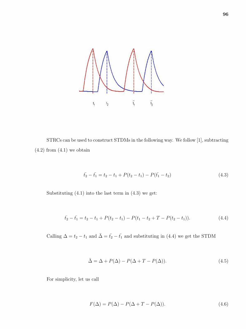
96
STRCs can be used to construct STDMs in the following way. We follow [1], subtracting
(4.2) from (4.1) we obtain
t2 − t1 = t2 − t1 + P (t2 − t1)− P (t1 − t2) (4.3)
Substituting (4.1) into the last term in (4.3) we get:
t2 − t1 = t2 − t1 + P (t2 − t1)− P (t1 − t2 + T − P (t2 − t1)). (4.4)
Calling ∆ = t2 − t1 and ∆ = t2 − t1 and substituting in (4.4) we get the STDM
∆ = ∆ + P (∆)− P (∆ + T − P (∆)). (4.5)
For simplicity, let us call
F (∆) = P (∆)− P (∆ + T − P (∆)). (4.6)

97
Thus the STDM (4.5) reads
∆ = ∆ + F (∆) (4.7)
The function F in (4.7) can be computed and the stability properties of the STDM
can be analyzed.
We can determine equilibrium solutions ∆0, which satisfies F (∆0) = 0 and describe
the time difference between the neurons at steady state.
Stable solutions for STDM satisfy:
−2 <d
d∆F < 0
STRCs and STDM have been used to investigate the synchronization properties of
coupled neurons [1], [4], [30], [28], [29].
In our Fitzhugh-Nagumo(FHN) model, because the ω-function has a synaptic-like
shape, Here we explore the possibility of using STDM methods to examine the stability
of any solutions.
v′k = f(vk) + γw − (1 + γαk)wk − γαjwj,
w′k = ε(αvk − λ− wk) k, j = 1, 2, j 6= k.
(4.8)
We refer to the period of an unperturbed oscillator as its natural period, T is the
natural period without forcing term:
v′k = f(vk) + γw − (1 + γαk)wk
w′k = ε(αvk − λ− wk)
(4.9)
When α1 6= α2, T1 is the period of first oscillator without the perturbation of the
second oscillator:
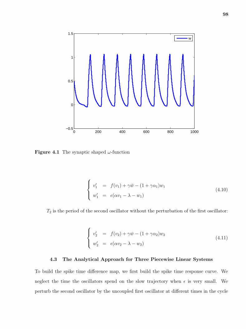
98
0 200 400 600 800 1000−0.5
0
0.5
1
1.5
w
Figure 4.1 The synaptic shaped ω-function
v′1 = f(v1) + γw − (1 + γα1)w1
w′1 = ε(αv1 − λ− w1)
(4.10)
T2 is the period of the second oscillator without the perturbation of the first oscillator:
v′2 = f(v2) + γw − (1 + γα2)w2
w′2 = ε(αv2 − λ− w2)
(4.11)
4.3 The Analytical Approach for Three Piecewise Linear Systems
To build the spike time difference map, we first build the spike time response curve. We
neglect the time the oscillators spend on the slow trajectory when ε is very small. We
perturb the second oscillator by the uncoupled first oscillator at different times in the cycle
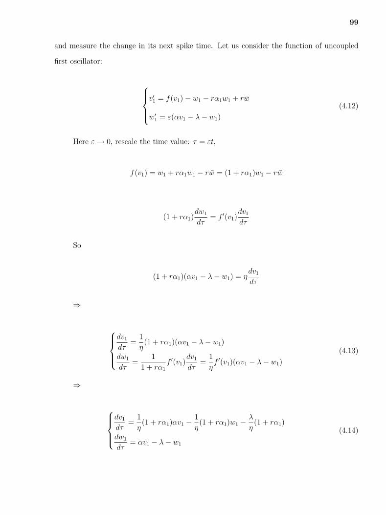
99
and measure the change in its next spike time. Let us consider the function of uncoupled
first oscillator:
v′1 = f(v1)− w1 − rα1w1 + rw
w′1 = ε(αv1 − λ− w1)
(4.12)
Here ε → 0, rescale the time value: τ = εt,
f(v1) = w1 + rα1w1 − rw = (1 + rα1)w1 − rw
(1 + rα1)dw1
dτ= f ′(v1)
dv1
dτ
So
(1 + rα1)(αv1 − λ− w1) = ηdv1
dτ
⇒
dv1
dτ=
1
η(1 + rα1)(αv1 − λ− w1)
dw1
dτ=
1
1 + rα1
f ′(v1)dv1
dτ=
1
ηf ′(v1)(αv1 − λ− w1)
(4.13)
⇒
dv1
dτ=
1
η(1 + rα1)αv1 − 1
η(1 + rα1)w1 − λ
η(1 + rα1)
dw1
dτ= αv1 − λ− w1
(4.14)

100
d
v1
w1
dτ=
αη(1 + rα1) − 1
η(1 + rα1)
α −1
v1
w1
+
−λ
η(1 + rα1)
−λ
So
d
v1
w1
dτ= T−1
λ1 0
0 λ2
T
v1
w1
+
−λ
η(1 + rα1)
−λ
dT
v1
w1
dτ=
λ1 0
0 λ2
T
v1
w1
+ T
−λ
η(1 + rα1)
−λ
T
v1
w1
=
v1
w1
Which derives:
dv1
dτ= λ1v1 − a1λ
η(1 + rα1)− b1λ
dw1
dτ= λ2w1 − c1λ
η(1 + rα1)− d1λ
(4.15)
In the case λ2 = 0,
d(λ1v1 − a1λη
(1 + rα1)− b1λ)
dτ= λ1(λ1v1 − a1λ
η(1 + rα1)− b1λ)
dw1
dτ= −c1λ
η(1 + rα1)− d1λ
(4.16)
w1 = −(c1λ
η(1 + rα1) + d1λ)τ + w1(0)
So
λ1v1 − a1λ
η(1 + rα1)− b1λ = k1e
λ1τ
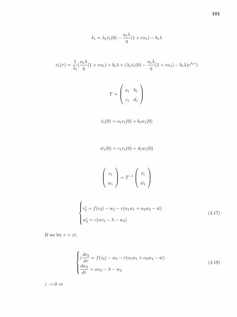
101
k1 = λ1v1(0)− a1λ
η(1 + rα1)− b1λ
v1(τ) =1
λ1
(a1λ
η(1 + rα1) + b1λ + (λ1v1(0)− a1λ
η(1 + rα1)− b1λ)eλ1τ )
T =
a1 b1
c1 d1
v1(0) = a1v1(0) + b1w1(0)
w1(0) = c1v1(0) + d1w1(0)
v1
w1
= T−1
v1
w1
v′2 = f(v2)− w2 − r(α1w1 + α2w2 − w)
w′2 = ε(αv2 − λ− w2)
(4.17)
If we let τ = εt,
εdv2
dτ= f(v2)− w2 − r(α1w1 + α2w2 − w)
dw2
dτ= αv2 − λ− w2
(4.18)
ε → 0 ⇒

102
f(v2) = w2 + r(α1w1 + α2w2 − w) = (1 + rα2)w2 + rα1w1 − rw
(1 + rα2)dw2
dτ= f ′(v2)
dv2
dτ− rα1
dw1
dτ
(1 + rα2)(αv2 − λ− w2) = ηdv2
dτ− rα1(αv1 − λ− w1)
dv2
dτ=
1
η((1 + rα2)(αv2 − λ− w2) + rα1(αv1 − λ− w1))
dw2
dτ= αv2 − λ− w2
(4.19)
d
v2
w2
dτ=
α(1+rα2)η
− (1+rα2)η
α −1
v2
w2
+
rα1
η(αv1 − λ− w1)− λ(1+rα2)
η
−λ
dT
v2
w2
dτ=
λ1 0
0 λ2
T
v2
w2
+ T
rα1
η(αv1 − λ− w1)− λ(1+rα2)
η
−λ
d
v2
w2
dτ=
λ1 0
0 λ2
v2
w2
+
s1
s2
If α1 = α2 = 0.5, λ2 = 0,
dv2
dτ= λ1v2 + s1,
dw2
dτ= s2
(4.20)
Here

103
s1 = a1(rα1
η(αv1 − λ− w1)− λ(1 + rα2)
η)− λb1
s2 = c1(rα1
η(αv1 − λ− w1)− λ(1 + rα2)
η)− λd1
v1(τ) = 1λ1
(a1λη
(1 + rα1) + b1λ + (λ1v1(0)− a1λη
(1 + rα1)− b1λ)eλ1τ )
w1(τ) = −( c1λη
(1 + rα1) + d1λ)τ + w1(0)
(4.21)
T−1 =
a′1 b′1
c′1 d′1
v1
w1
= T−1
v1
w1
=
a′1 b′1
c′1 d′1
v1
w1
v1(τ) is a linear combination of eλ1τ and 1, w1(τ) is a linear combination of τ and 1.
v1 and w1 are linear combination of v1 and w1, so v1 and w1 are linear combination of eλ1τ ,
τ and 1. s1 and s2 are also linear combination of eλ1τ , τ and 1.
dv2
dτ= λ1v2 + aeλ1τ + bτ + c
If we make v2 = eλ1τf ,
dv1
dτ= λ1e
λ1τf + eλ1τf ′ = λ1eλ1τf + aeλ1τ + bτ + c
f ′ = e−λ1τ (aeλ1τ + bτ + c) = a + bτe−λ1τ + ce−λ1τ

104
f = aτ − bτ
λ1
e−λ1τ − b
λ21
e−λ1τ − c
λ1
e−λ1τ + s
s = v1(0) +b
λ21
+c
λ1
so
v1 = aτeλ1τ − bτ
λ1
+ v1(0)
dw2
dτ= aeλ1τ + bτ + c
w2 =a
λ1
eλ1τ +bτ 2
2+ cτ + w2(0)− a
λ1
4.4 Comparison of Numerical and Analytical Results
We can numerically and analytically compute the effect of perturbation of the second
oscillator with respect to the first oscillator and build the spike time response curve and
spike time response map and compare these results. The error between the two curves is
close to 0.
Consider the piecewise-linear systems, here are two examples:
When α1 = 0.3, α2 = 0.7, if λ ≥ 1.4, we can get in phase pattern, however, if λ ≤ 1.3,
we get out of phase-pattern. In the Spike time difference map, when λ = 1.4, the slope of
STDM at the two endpoints are negative, and if λ = 1.3, the slope of STDM at the endpoints
are non-negative.
When α1 = 0.2, α2 = 0.8, if λ ≥ 1, we can get in phase pattern, however, if λ ≤ 0.9, we
get out of phase-pattern. In the Spike time difference map, when λ = 1, the slope of STDM
at the two endpoints are negative, and if λ = 0.9, the slope of STDM at the endpoints are
non-negative.

105
0 50 100 150−20
−15
−10
−5
0
5
10
15
20
numerical and analytical STDM: γ=0.1;λ=0.5;ε=0.005;α=4;α1=α
2=0.5
numercal STDManalytical STDMerror between two curves
If the slope of the STDM between -2 and 0 , the two oscillators are stable. When the
slope of STDM is negative, the pattern is stable. When α1 = 0.3, α2 = 0.7, if λ ≥ 1.4, we
get in phase pattern. When α1 = 0.2, α2 = 0.8, if λ ≥ 1, we get in phase pattern. So the
result using STDM method is consistent in the phase figures Fig. 4.3 and Fig. 4.4.
For cubic systems, here are also two examples:
When α1 = 0.5, α2 = 0.5, if λ > 0.45, we can get in phase pattern, however, if λ ≤ 0.45,
we get out of phase-pattern. In Fig. 4.6, the Spike time difference map shows that when
λ = 0.5, the slope of STDM at the two endpoints are negative, and if λ = 0.45, the slope of
STDM at the endpoints are non-negative.
For α1 = 0.3, α2 = 0.7, if λ > 0.25, we can get in phase pattern, however, if λ ≤ 0.25,
we get out of phase-pattern. In Fig. 4.8, the Spike time difference map shows that when
λ = 0.3, the slope of STDM at the two endpoints are negative, and if λ = 0.25, the slope of
STDM at the endpoints are non-negative.
These examples shows that the result of phases by using STDM method is consistent
with the result in the phase picture. So we can use the STDM method to estimate the

106
Figure 4.2 The phase of two piecewise-linear oscillators system with parameters: γ =0.1,ε = 0.005,α = 4
0 20 40 60 80 100 120−6
−4
−2
0
2
4
6
8
10
12
14
STDM:γ=0.1;ε=0.005;α=4;α1=0.3;α
2=0.7,λ=1.4
0 50 100 150−20
−15
−10
−5
0
5
10
15
20
STDM:γ=0.1;ε=0.005;α=4;α1=0.3;α
2=0.7,λ=1.3
Figure 4.3 The spike time difference map of two piecewise-linear oscillators withparameters: γ = 0.1,ε = 0.005,α = 4,α1 = 0.3,α2 = 0.7, λ = 1.4 and λ = 1.3

107
0 20 40 60 80 100 120−4
−2
0
2
4
6
8
10
12
14
16
STDM:γ=0.1;ε=0.005;α=4;α1=0.2;α
2=0.8,λ=1.
0 20 40 60 80 100 120 140−20
−15
−10
−5
0
5
10
15
20
STDM:γ=0.1;ε=0.005;α=4;α1=0.2;α
2=0.8,λ=0.9
Figure 4.4 The spike time difference map of two piecewise-linear oscillators withparameters: γ = 0.1,ε = 0.005,α = 4,α1 = 0.2,α2 = 0.8, λ = 1 and λ = 0.9
0 0.5 1 1.5 2 2.5 3
0
0.2
0.4
0.6
0.8
1
λ
phas
e
cubic:γ=0.1, ε=0.005, α=4
α
1=0.2, α
2=0.8
α1=0.3, α
2=0.7
α1=0.4, α
2=0.6
α1=0.5, α
2=0.5
Figure 4.5 The phase of two cubic oscillators system with parameters: γ = 0.1,ε =0.005,α = 4

108
0 20 40 60 80 100 120 140 160−8
−6
−4
−2
0
2
4
6
8
0 20 40 60 80 100 120 140 160 180−15
−10
−5
0
5
10
15
Figure 4.6 The spike time difference map of two cubic oscillators with parameters:γ = 0.1,ε = 0.005, α = 4, α1 = 0.5, α2 = 0.5, λ = 0.5 and λ = 0.45
0 20 40 60 80 100 120 140−2
0
2
4
6
8
10
12
0 20 40 60 80 100 120 140 160 180−40
−30
−20
−10
0
10
20
Figure 4.7 The spike time difference map of two cubic oscillators with parameters:γ =0.1,ε = 0.005,α = 4,α1 = 0.3,α2 = 0.7, λ = 0.3 and λ = 0.25
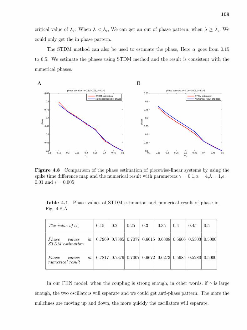
109
critical value of λc: When λ < λc, We can get an out of phase pattern; when λ ≥ λc, We
could only get the in phase pattern.
The STDM method can also be used to estimate the phase, Here α goes from 0.15
to 0.5. We estimate the phases using STDM method and the result is consistent with the
numerical phases.
A B
0.1 0.15 0.2 0.25 0.3 0.35 0.4 0.45 0.50.5
0.55
0.6
0.65
0.7
0.75
0.8
0.85
α1
phas
e
phase estimate: γ=0.1,ε=0.01,α=4,λ=1
STDM estimationNumerical result of phase
0.1 0.15 0.2 0.25 0.3 0.35 0.4 0.45 0.50.5
0.55
0.6
0.65
0.7
0.75
0.8
0.85
α1
phas
e
phase estimate: γ=0.1,ε=0.005,α=4,λ=1
STDM estimationNumerical result of phase
Figure 4.8 Comparison of the phase estimation of piecewise-linear systems by using thespike time difference map and the numerical result with parameters:γ = 0.1,α = 4,λ = 1,ε =0.01 and ε = 0.005
Table 4.1 Phase values of STDM estimation and numerical result of phase inFig. 4.8-A
The value of α1 0.15 0.2 0.25 0.3 0.35 0.4 0.45 0.5
Phase values inSTDM estimation
0.7969 0.7385 0.7077 0.6615 0.6308 0.5606 0.5303 0.5000
Phase values innumerical result
0.7817 0.7379 0.7007 0.6672 0.6273 0.5685 0.5280 0.5000
In our FHN model, when the coupling is strong enough, in other words, if γ is large
enough, the two oscillators will separate and we could get anti-phase pattern. The more the
nullclines are moving up and down, the more quickly the oscillators will separate.

110
Table 4.2 Phase values of STDM estimation and numerical result of phase inFig. 4.8-B
The value of α1 0.15 0.2 0.25 0.3 0.35 0.4 0.45 0.5
Phase values inSTDM estimation
0.7623 0.7131 0.6748 0.6423 0.6048 0.5564 0.5280 0.5000
Phase values innumerical result
0.7718 0.7264 0.6879 0.6539 0.6181 0.5567 0.5264 0.5000
We know that in STDM, the more the slope of the middle point of the STDM is close
to value −1, the more quickly two oscillators will separate. In Fig. 4.9, the slope of the
middle point of the curve in the STDM approaching to −1 by increasing the value of γ, so
two oscillators separate more quickly by increasing the value of γ. That’s because that the
extend the V -nullclines moving up and down is increasing by increasing the value of γ. That
makes the ”moving nullclines” strong enough to make the second oscillator stay around the
point v = 0 for more time while the first oscillator moves on to the right branch, which
makes the two oscillators separate more quickly.
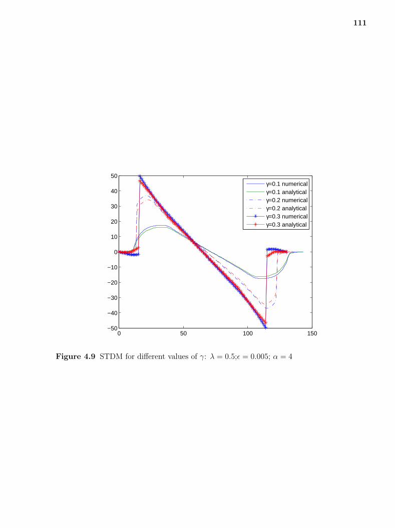
111
0 50 100 150−50
−40
−30
−20
−10
0
10
20
30
40
50
γ=0.1 numericalγ=0.1 analyticalγ=0.2 numericalγ=0.2 analyticalγ=0.3 numericalγ=0.3 analytical
Figure 4.9 STDM for different values of γ: λ = 0.5;ε = 0.005; α = 4
CHAPTER 5
CONCLUSION
5.1 Summary of Results and Discussion
The Kuramoto model describes the synchronization behavior of a large population of coupled
limit-cycle oscillators whose natural frequencies satisfy some certain distribution. The
Kuramoto model predicts that, if the oscillators have strong coupling, they will become
phase-locked. Kuramoto gave an estimate for the distribution for the order parameter,
but the order parameter has an error from Kuramoto’s estimation. My research involved
studying the basics of Kuramoto’s analysis and then investigating how the order parameter
is distributed around Kuramoto’s estimation by given different initial conditions.
The Belousov-Zhabotinsky reaction is a laboratory example of pattern formation in a
chemical system that involves nothing more than chemical reaction and molecular diffusion.
The FitzHugh-Nagumo (FHN) model is a generic model for excitable media and can be
applied to a variety of systems, most notably chemistry, biology and neuroscience. My
research focuses on the synchronization of FHN model. I use piecewise linear systems to
approximate the cubic systems in FHN model. In both cases, the ‘motion’ of the nullclines
cause the two oscillators to separate. Especially, when the value of γ is large enough, the
‘moving nullcline’ is strong enough to make the second oscillator stay around the origin for
a while and the two oscillators separate.
The nervous system is a very efficient and massively parallel computational device.
Models may capture this property to solve a certain class of problems. The system contains
only 302 neurons, and it forms about 7000 chemical synapses. The synapses are the
connections made by an axon to another neuron. When an action potential arrives at a
synapse from the postsynaptic cell, neurotransmitter is released into the synaptic cleft. The
neurotransmitter will interact with ion channels on the membrane of the postsynaptic cell
causing them to open letting some ions into the cell while letting other ions escape. In [1]
and [32], they use a synaptic perturbation on the timing of subsequent spikes to predict
the behavior of synchronization of neurons. Changes in firing times depend nonlinearly
112
on synaptic strength. They apply ”spike time response methods” on the model. In our
model, there are two oscillators coupled with each other. We don’t have the synaptic input.
However, the coupling term includes the w-function, which has a synaptic-like shape, so we
can also use the spike time response method. The spike time response method can predict
oscillatory patterns and the values of phases.
5.2 Future Work
There are several open questions in these problems which are very interesting and useful to
consider.
In the present work of Kuramoto model, we explored the distribution of the order
parameter of the Kuramoto model without noise terms. We still need to see how the order
parameter changes with the noise term. We only numerically verified the locked terms and
the unlocked terms, which are independent. Works have to be continued on seeing whether
analytical proof is possible.
In the project of Belousov-Zhabotinsky (BZ) reaction, we focused on a system of two
oscillators, systems of three and more oscillators should be explored in the future. We
only tried three piecewise linear approximations, In the future, it is possible to increase the
number of linear pieces to produce a better approximation.
113

APPENDIX A
PROOFS AND EXAMPLES
A.1 Proof of Lemma 1
Proof
v1′
v2′
ω1′
ω2′
= D
v1
v2
ω1
ω2
+ L
Because the matrix D can be diagonalized:
D =
a 0 −(1 + γα1) −γα2
0 b −γα1 −(1 + γα2)
εα 0 −ε 0
0 εα 0 −ε
= A
λ1 0 0 0
0 λ2 0 0
0 0 λ3 0
0 0 0 λ4
A−1
Plug D into the above equation and multiply both sides by A−1:
A−1
v1′
v2′
ω1′
ω2′
=
λ1 0 0 0
0 λ2 0 0
0 0 λ3 0
0 0 0 λ4
A−1
v1
v2
ω1
ω2
+ A−1L
If we let
A−1
v1
v2
ω1
ω2
=
v1
v2
ω1
ω2
114

115
Then
v1′
v2′
ω1′
ω2′
=
λ1 0 0 0
0 λ2 0 0
0 0 λ3 0
0 0 0 λ4
v1
v2
ω1
ω2
+ A−1L
⇒
λ1 0 0 0
0 λ2 0 0
0 0 λ3 0
0 0 0 λ4
v1
v2
ω1
ω2
+ A−1L
′
=
λ1 0 0 0
0 λ2 0 0
0 0 λ3 0
0 0 0 λ4
v1′
v2′
ω1′
ω2′
=
λ1 0 0 0
0 λ2 0 0
0 0 λ3 0
0 0 0 λ4
λ1 0 0 0
0 λ2 0 0
0 0 λ3 0
0 0 0 λ4
v1
v2
ω1
ω2
+ A−1L
⇒
λ1 0 0 0
0 λ2 0 0
0 0 λ3 0
0 0 0 λ4
v1
v2
ω1
ω2
+ A−1L

116
=
eλ1t 0 0 0
0 eλ2t 0 0
0 0 eλ3t 0
0 0 0 eλ4t
λ1 0 0 0
0 λ2 0 0
0 0 λ3 0
0 0 0 λ4
v1(0)
v2(0)
ω1(0)
ω2(0)
+ A−1L
=
eλ1t 0 0 0
0 eλ2t 0 0
0 0 eλ3t 0
0 0 0 eλ4t
λ1 0 0 0
0 λ2 0 0
0 0 λ3 0
0 0 0 λ4
A−1
v1(0)
v2(0)
ω1(0)
ω2(0)
+ A−1L
⇒
A−1
v1
v2
ω1
ω2
=
v1
v2
ω1
ω2
=
1λ1
0 0 0
0 1λ2
0 0
0 0 1λ3
0
0 0 0 1λ4
·
eλ1t 0 0 0
0 eλ2t 0 0
0 0 eλ3t 0
0 0 0 eλ4t
λ1 0 0 0
0 λ2 0 0
0 0 λ3 0
0 0 0 λ4
A−1
v1(0)
v2(0)
ω1(0)
ω2(0)
+ A−1L
− A−1L
⇒

117
v1
v2
ω1
ω2
= A
1λ1
0 0 0
0 1λ2
0 0
0 0 1λ3
0
0 0 0 1λ4
·
eλ1t 0 0 0
0 eλ2t 0 0
0 0 eλ3t 0
0 0 0 eλ4t
λ1 0 0 0
0 λ2 0 0
0 0 λ3 0
0 0 0 λ4
A−1
v1(0)
v2(0)
ω1(0)
ω2(0)
+ A−1L
− A−1L
A.2 Proof of Lemma 3.6.1
Proof Consider the moving v-nullclines function (3.8):
wk =f(vk) + γ w
1 + αkγ− γ αjwj
1 + αkγ
The above function f(v), parameters ω, αk,γ are all fixed, it is the term −γαjωj that
makes the v-nullcline moving. The v-nullcline of (vk, ωk) is moving up(down) is equivalent
to ω′k positive(ω′k negative) for any value of vk fixed. It is also equivalent to −γαjωj
increasing(decreasing), it is equivalent to ωj′ = αvj − λ− ωj positive (negative).
The position of the point(vj, ωj) determines whether it is positive, zero, or negative:
(i) When the point (vj, ωj) lies on the left side of ω nullcline, ω′j = αjv − λj − ωj < 0,
(ii) When the point (vj, ωj) lies on the ω nullcline, ω′j = αjv − λj − ωj = 0,
(iii) When the point (vj, ωj) lies on the right side of ω nullcline, ω′j = αjv − λj − ωj > 0.
So whether the nullcline of one oscillator (vk, ωk) is moving up (moving down) is
determined by the position of the other oscillator (vj, ωj), if the other oscillator lies on

118
the left side of ω-nullcline, the v-nullcline of the oscillator (vk, ωk) move up; if the other
oscillator lies on the right side of ω-nullcline, the v-nullcline of this oscillator (vk, ωk) move
down.

119
A.3 Example of Piecewise-linear Oscillators
A B
−1 −0.5 0 0.5 1 1.5 2−0.2
0
0.2
0.4
0.6
0.8
1
1.2
1.4
V
W
t=0
w nullclinev1 nullclinev2 nullclineoscillator 1oscillator 2
−1 −0.5 0 0.5 1 1.5 2−0.2
0
0.2
0.4
0.6
0.8
1
1.2
1.4
t=40
V
W
C D
−1 −0.5 0 0.5 1 1.5 2−0.2
0
0.2
0.4
0.6
0.8
1
1.2
1.4
t=97
V
W
−1 −0.5 0 0.5 1 1.5 2−0.2
0
0.2
0.4
0.6
0.8
1
1.2
1.4
t=103
V
W

120
E F
−1 −0.5 0 0.5 1 1.5 2−0.2
0
0.2
0.4
0.6
0.8
1
1.2
1.4
t=108
V
W
−1 −0.5 0 0.5 1 1.5 2−0.2
0
0.2
0.4
0.6
0.8
1
1.2
1.4
t=128
V
W
G H
−1 −0.5 0 0.5 1 1.5 2−0.2
0
0.2
0.4
0.6
0.8
1
1.2
1.4
t=134
V
W
−1 −0.5 0 0.5 1 1.5 2−0.2
0
0.2
0.4
0.6
0.8
1
1.2
1.4
t=137
V
W
I J
−1 −0.5 0 0.5 1 1.5 2−0.2
0
0.2
0.4
0.6
0.8
1
1.2
1.4
t=157
V
W
−1 −0.5 0 0.5 1 1.5 2−0.2
0
0.2
0.4
0.6
0.8
1
1.2
1.4
t=161
V
W

121
K L
−1 −0.5 0 0.5 1 1.5 2−0.2
0
0.2
0.4
0.6
0.8
1
1.2
1.4
t=186
V
W
−1 −0.5 0 0.5 1 1.5 2−0.2
0
0.2
0.4
0.6
0.8
1
1.2
1.4
t=192
V
W
Figure A.1 Two globally coupled oscillators moving with equation (3.11)in piecewise-linearcase, and two out of phase clusters for the following parameters: α = 3, γ = 0.1, α1 =0.5, α2 = 0.5
A B
−1 −0.5 0 0.5 1 1.5 2−0.2
0
0.2
0.4
0.6
0.8
1
1.2
1.4
V
W
t=0
w nullclinev1 nullclinev2 nullclineoscillator 1oscillator 2
−1 −0.5 0 0.5 1 1.5 2−0.2
0
0.2
0.4
0.6
0.8
1
1.2
1.4
t=48
V
W
C D
−1 −0.5 0 0.5 1 1.5 2−0.2
0
0.2
0.4
0.6
0.8
1
1.2
1.4
t=65
V
W
−1 −0.5 0 0.5 1 1.5 2−0.2
0
0.2
0.4
0.6
0.8
1
1.2
1.4
t=76
V
W

122
E F
−1 −0.5 0 0.5 1 1.5 2−0.2
0
0.2
0.4
0.6
0.8
1
1.2
1.4
t=82
V
W
−1 −0.5 0 0.5 1 1.5 2−0.2
0
0.2
0.4
0.6
0.8
1
1.2
1.4
t=105
V
W
G H
−1 −0.5 0 0.5 1 1.5 2−0.2
0
0.2
0.4
0.6
0.8
1
1.2
1.4
t=110
V
W
−1 −0.5 0 0.5 1 1.5 2−0.2
0
0.2
0.4
0.6
0.8
1
1.2
1.4
t=112
V
W
I J
−1 −0.5 0 0.5 1 1.5 2−0.2
0
0.2
0.4
0.6
0.8
1
1.2
1.4
t=127
V
W
−1 −0.5 0 0.5 1 1.5 2−0.2
0
0.2
0.4
0.6
0.8
1
1.2
1.4
t=132
V
W

123
K L
−1 −0.5 0 0.5 1 1.5 2−0.2
0
0.2
0.4
0.6
0.8
1
1.2
1.4
t=161
V
W
−1 −0.5 0 0.5 1 1.5 2−0.2
0
0.2
0.4
0.6
0.8
1
1.2
1.4
t=164
V
W
Figure A.2 Two globally coupled oscillators moving with equation (3.11), and two out ofphase clusters for the following parameters: α = 3, γ = 0.1, α1 = 0.5, α2 = 0.5
0 200 400 600 800 1000−1
−0.5
0
0.5
1
1.5
2
t
V
FHN
V1V2
400 600 800 1000 1200 1400−1
−0.5
0
0.5
1
1.5
2
t
V
FHN−PWL
Figure A.3 Two globally coupled oscillators moving with equation (3.11), and two anti-phase clusters for the following parameters: α = 3, γ = 0.1, α1 = 0.5, α2 = 0.5
REFERENCES
[1] C. D. Acker, N. Kopell, and J. A. White. Synchronization of strongly coupled excitatoryneurons: relating network behavior to biophysics. J Comput Neurosci, 15(1):71–90,2003.
[2] B. P. Belousov. A periodic reaction and its mechanism. Compilation of Abstracts onRadiation Medicine (Med. Publ., Moscow), 147:145, 1959.
[3] R. J. Belousov, B. P.& in Field and Burger. A periodic reaction and its mechanism;Oscillations and traveling waves in chemical systems. Wiley, New York, 1985.
[4] Yassine Boubendir, Vicenc Mendez, and Horacio G. Rotstein. Dynamics of one- andtwo-dimensional fronts in a bistable equation with time-delayed global feedback:Propagation failure and control mechanisms. Physical Review E, 82(3):036601+, Sep2010.
[5] J.C. Butcher. The Numerical Analysis of Ordinary Differential Equations:Runge-Kutta andGeneral Linear Methods. Wiley, 1987.
[6] John Charles Butcher. Numerical methods for ordinary differential equations. Wiley, 2008.
[7] D. T. W. Chick, S. Coombes, and Z. D. Wang. Clustering through post inhibitory reboundin synaptically coupled neurons. Phys. Rev. E 70, 011908, 70:Issue 1, 2004.
[8] S. Coombes. Phase locking in networks of synaptically-coupled mckean relaxation oscillators.Physicad, 160:173–188, 2008.
[9] Christopher M. Dobson. Protein folding and disease: a view from the first horizonsymposium. Nat Rev Drug Discov, 2(2):154–160, February 2003.
[10] J. A. Epstein, I. R.; Pojman. An introduction to nonlinear chemical dynamics: Oscillations,waves, patterns, and chaos. J. Chem. Educ., 77 (4):450, 2000.
[11] R. J. Fields, E. Koros, and R. M. Noyes. Oscillations in chemical systems. 2. thoroughanalysis of temporal oscillation in bromate-cerium-malonic acid system. Jamchemsoc,94:8649–8664, 1972.
[12] R. Fitzhugh. Impulses and physiological states in theoretical models of nerve membrane.Biophysical Journal, 1(6):445–466, July 1961.
[13] Richard FitzHugh. Mathematical models of threshold phenomena in the nerve membrane.Bulletin of Mathematical Biology, 17(4):257–278, December 1955.
[14] D. Golomb, D. Hansel, B. Shraiman, and H. Sompolinksy. Clustering in globally coupledphase oscillators. pra, 45:3516–3530, 1992.
[15] A. Zhabotinsky H. G. Rotstein, N. Kopell and I. R. Epstein. A canard mechanism forlocalization in systems of globally coupled oscillators. SIAM J. Appl. Math., 63:1998C2019, 2003.
124
125
[16] D. Hansel, G. Mato, and C. Meunier. Synchrony in Excitatory Neural Networks. NeuralComputation, 7(2):307–337, March 1995.
[17] Eugene M. Izhikevich. Dynamical systems in neuroscience: the geometry of excitability andbursting. Computational neuroscience. MIT Press, 2007.
[18] O. Jensen, P. Goel, N. Kopell, M. Pohja, R. Hari, and B. Ermentrout. On the humansensorimotor-cortex beta rhythm: sources and modeling. Neuroimage, 26(2):347–355,June 2005.
[19] Conrad J Perez Vicente Felix Ritort Renato Spigler Juan A.Acebron, L.L.Bonilla. Thekuramoto model: A simple parpadigm for synchronization phenomena. Reviews ofModern Physics, 77(1):137C185, January 2005.
[20] J. Keener and J. Sneyd. Mathematical Physiology. Springer-Verlag, 1998.
[21] N. Kopell and G. Ermentrout. Mechanisms of phase-locking and frequency control in pairsof coupled neural oscillators, 2000.
[22] Yoshiki Kuramoto. Chemical oscillations, waves, and turbulence. Springer-Verlag, NewYork, 1984.
[23] H. P. McKean. Nagumo’s equation. Advances in Mathematics, 4:209–223, 1970.
[24] Renato E. Mirollo and Steven H. Strogatz. Synchronization of pulse-coupled biologicaloscillators. SIAM Journal on Applied Mathematics, 50(6):1645–1662, 1990.
[25] JD Murray. Mathematical Biology: an Introduction. Springer, 2002.
[26] J. D. Murry. Mathematical Biology: I. An Introduction (Interdisciplinary AppliedMathematics). Springer; 3rd edition, December 8, 2007.
[27] J. Nagumo, S. Arimoto, and S. Yoshizawa. An active pulse transmission line simulatingnerve axon. Proceedings of the IRE, 50(10):2061–2070, October 1962.
[28] Theoden Netoff, Corey Acker, Jonathan Bettencourt, and John White. Beyond Two-CellNetworks: Experimental Measurement of Neuronal Responses to Multiple SynapticInputs. Journal of Computational Neuroscience, 18(3):287–295, June 2005.
[29] Theoden I. Netoff, Robert Clewley, Scott Arno, Tara Keck, and John A. White. Epilepsy inSmall-World Networks. J. Neurosci., 24(37):8075–8083, September 2004.
[30] Myongkeun Oh and Victor Matveev. Loss of phase-locking in non-weakly coupled inhibitorynetworks of type-I model neurons. Journal of Computational Neuroscience.
[31] S. A. Oprisan, A. A. Prinz, and C. C. Canavier. Phase resetting and phase locking in hybridcircuits of one model and one biological neuron. Biophys J, 87(4):2283–2298, October2004.
[32] D. D. Pervouchine, T. I. Netoff, H. G. Rotstein, J. A. White, M. O. Cunningham, M. A.Whittington, and N. J. Kopell. Low-dimensional maps encoding dynamics in entorhinalcortex and hippocampus. Neural Comput, 18(11):2617–2650, November 2006.

126
[33] J. Rinzel and J. B. Keller. Traveling wave solutions of a nerve conduction equation. Physicad,13:1313–1337, 1973.
[34] H. G. Rotstein, N. Kopell, A. Zhabotinsky, and I. R. Epstein. A canard mechanism forlocalization in systems of globally coupled oscillators. Siamap, 63:1998–2019, 2003.
[35] H. G. Rotstein, N. Kopell, A. Zhabotinsky, and I. R. Epstein. Canard phenomenon andlocalization of oscillations in the belousov-zhabotinsky reaction with global feedback.JCHP, 119 (17):8824–8832, 2003.
[36] F. Sagues and I. R Epstein. Nonlinear chemical dynamics. Dalton Trans, 1:1201–1217, 2003.
[37] RM Schoen. The existence of weak solutions with prescribed singular behavior fora conformally invariant scalar equation. Communications on pure and appliedmathematics, 41, no. 3:317–392, 1988.
[38] Roy M. Smeal, G. Bard Ermentrout, and John A. White. Phase-response curves andsynchronized neural networks. Philosophical Transactions of the Royal Society B:Biological Sciences, 365(1551):2407–2422, August 2010.
[39] S. H. Strogatz. Sync: the emerging science of spontaneous order. Hyperion, New York, 2003.
[40] Steven H. Strogatz. From kuramoto to crawford: exploring the onset of synchronization inpopulations of coupled oscillators. Physica D, 143:1–20, September 2000.
[41] Steven Henry Strogatz. Nonlinear Dynamics and Chaos with Applications to Physics,Biology, Chemistry, and Engineering. Addison-Wesley, Reading, MA, 1994.
[42] A. Tonnelier. The mckean’s caricature of the fitzhugh-nagumo model. the space-clampedsystem. Siap, 63:459–484, 2002.
[43] V. K. Vanag, L. Yang, M. Dolnik, and Epstein I. R. Zhabotinsky, A. M. Oscillatorycluster patterns in a homogeneous chemical system with global feedback. Nature,406:(6794):389–391, 2000.
[44] V. K. Vanag, A. M. Zhabotinsky, and I. R. Epstein. Pattern formation in the belusov-zhabotinsky reaction with photochemical global feedback. JCHP, 104A:11566–11577,2000.
[45] V. K. Vanag, A. M. Zhabotinsky, and I. R. Epstein. Oscillatory clusters in the periodicallyilluminated, spatially extended belousov-zhabotinsky reaction. PRL, 86:3, 2001.
[46] W. P. Wang. Multiple impulse solutions to mckean’s caricature of the nerve equation. 2.stability. Communications on pure and applied mathematics, 41:997–1025, 1988.
[47] Arthur T. Winfree. The Geometry of Biological Time. Springer, 2nd edition, June 2001.
[48] N. Zaikin and Zhabotinsky. Concentration wave propagation in two-dimensional liquid-phaseself-oscillating system. Nature, 225:535–537, 1970.

127
[49] Daniel E. Zak, Haiping Hao, Rajanikanth Vadigepalli, Gregory M. Miller, Babatunde A.Ogunnaike, and James S. Schwaber. Systems analysis of circadian time-dependentneuronal epidermal growth factor receptor signaling. Genome Biology, 7:R48+, June2006.
[50] A. M. Zhabotinksy. Periodic processes of malonic acid oxidation in a liquid phase. Biofizika,9:306–311, 1964.
[51] A. M. Zhabotinksy. Belousov-zhabotinsky reaction. Scholarpedia, 2:1435, 2007.
[52] A. M. Zhabotinsky, F. Buchholtz, A. B. Kiyatkin, and I. R. Epstein. Oscillations and wavesin metal-ion-catalyzed bromate oscillating reactions in highly oxidized states. JCHP,97:7578–7584, 1993.