corporate asset purchases and sales: theory and...
TRANSCRIPT

ARTICLE IN PRESS
0304-405X/$ - s
doi:10.1016/j.jfi
$This paper
project benefite
Bond, and sem
2007 Midwest
University, Un
comments from
The views expr
staff.�CorrespondE-mail addr
Journal of Financial Economics 87 (2008) 471–497
www.elsevier.com/locate/jfec
Corporate asset purchases and sales: Theory and evidence$
Missaka Warusawitharana�
Division of Research and Statistics, Board of Governors of the Federal Reserve System, Washington, DC 20551, USA
Received 20 May 2006; received in revised form 30 January 2007; accepted 27 February 2007
Available online 19 November 2007
Abstract
Purchases and sales of operating assets by firms generated $162 billion for shareholders over the past 20 years. This
contrasts sharply with the evidence on mergers. This paper characterizes the behavior of value-maximizing firms, which
could grow organically, purchase existing assets, or sell assets. The approach yields an endogenous selection model that
links asset purchases and sales to fundamental properties of the firm. Empirical tests confirm the predictions of the model.
In particular, return on assets and size strongly predict when firms purchase or sell assets, and the transaction size covaries
with the value of capital employed by the firm. These findings indicate that corporate asset purchases and sales are
consistent with efficient investment decisions.
Published by Elsevier B.V.
JEL classification: G31; G34
Keywords: Acquisitions; Asset sales; Tobin’s Q; Selection models
1. Introduction
Firms regularly trade product lines, operations in a specific locale, subsidiaries, and other business units.Approximately $100 billion worth of assets were transacted between firms in 2004. From 1985 onward, these
ee front matter Published by Elsevier B.V.
neco.2007.02.005
is part of my dissertation at the Wharton School. I wish to thank my chair Joao Gomes for invaluable guidance. The
d substantially from conversations with Andrew Abel, Gary Gorton, Jessica Wachter, Amir Yaron, Ronald Masulis, Philip
inar participants at the financial constraints or technological differences conference at Pennsylvania State University, the
Finance Association meeting, the 2007 Western Finance Association meeting, the Federal Reserve Board, Temple
iversity of Wisconsin-Madison, Vanderbilt University and the Wharton School. I gratefully acknowledge valuable
an anonymous referee. I thank David Cho and Elizabeth Holmquist for providing excellent research assistant support.
essed in this paper are mine and do not reflect the views of the Board of Governors of the Federal Reserve System or its
ing author.
ess: [email protected]

ARTICLE IN PRESSM. Warusawitharana / Journal of Financial Economics 87 (2008) 471–497472
transactions led to a net gain of $162 billion for shareholders in participating firms.1 This suggests that assettransactions improve the allocative efficiency of capital in the economy.
This paper argues that firms’ investment needs drive their decisions to grow organically or inorganically.Firms that wish to grow rapidly do so through acquisitions, and firms aiming for slower growth do so throughinternal investments. Further, firms downsize when they find themselves with surplus assets. Essentially,acquisitions and asset sales are driven by choices over the scale of the firm. Alternative theories that arguethese decisions are driven by decisions over the scope of the firm include the transactions cost economicsapproach (see Williamson, 1975; Klein, Crawford, and Alchian, 1978), and the property rights approach(see Grossman and Hart, 1986; Hart and Moore, 1990).
This study presents and tests a model in which asset purchases and sales enable the transfer of capital fromless productive to more productive firms. These transactions occur as part of the overall investment decisionsof value-maximizing firms. The theoretical development produces an endogenous selection model that linksasset purchases and sales to fundamentals of the firm. The empirical analysis builds on the theoretical resultsand employs logit regressions and selection models to test the predictions of the model. The key findings arethat return on assets and size strongly influence the choice of a firm to purchase or sell existing assets and thatconditional on the decision to engage in a transaction, firms with high growth opportunities buy more assets.
The model builds on the Q-theoretic framework for investment (see Lucas, 1967; Hayashi, 1982; Abel,1983). The model economy consists of a large number of firms with heterogeneous profitability. Decreasingreturns to scale lead managers to vary the size of the firm as profitability varies exogenously. The keyeconomic idea is that firms engage in asset purchases and sales to move the firm toward its optimal size, whichvaries with profitability.
Transaction costs keep firms from buying existing assets until desired investment exceeds a threshold.However, when a firm elects to purchase (sell) existing assets, the marginal value of capital inside the firmmust equal the marginal cost (payoff) of the transaction. This yields a selection model in which the quantityof assets traded depends on marginal Q, while the choice of purchasing or selling assets depends onfirm characteristics. The model identifies profitability and firm size as the key determinants of the choice offirms to buy and sell existing assets. Given size, optimal investment rises with profitability, and highlyprofitable firms engage in asset purchases. Conversely, less profitable firms find it optimal to downsize and sellexisting assets.
This paper focuses on the productivity-driven decision of firms to seek organic growth, acquisitions, or assetsales.2 As such, it is closely related to the work of Jovanovic and Rousseau (2002), who argue that mergers canbe viewed as acquisitions of unproductive assets by firms with high productivity. At a more disaggregatedlevel, Maksimovic and Phillips (2001) study plant sales between firms and find that transactions improve theallocation of resources. Eisfeldt and Rampini (2006) use a productivity-based approach to study asset salesand acquisitions at the macro level. A recent paper by Yang (2006) demonstrates that a neo-classical model ofasset transactions can explain return characteristics and pro-cyclical transaction volumes. Other papers thatuse an investment-based approach to study aspects of corporate finance include Gomes and Livdan (2004),Hennessy and Whited (2005), and Hennessy, Levy, and Whited (2007).
The empirical analysis employs a comprehensive set of asset purchases and sales obtained from theSecurities Data Corporation (SDC) Platinum mergers and acquisitions database.3 This database containsinformation on asset purchases and sales by public firms, their subsidiaries, and private firms. The data setprovides extensive coverage on these transactions in the United States, recording more than ten thousandcompleted asset transactions involving public firms or their subsidiaries over the past 20 years. Prior studies onasset sales by Lang, Poulson, and Stulz (1995) and Bates (2005) analyze much smaller samples.
1These values are obtained using the sample of asset transactions subsequently analyzed in the paper. In comparison, Moeller,
Schlingemann, and Stulz (2005) report that the total value creation to shareholders in mergers totaled $55 billion from 1981 to 1998 and is
negative from 1981 to 2002.2Other potential reasons for acquisitions include maturing product lines, regulatory limits, and value creation through horizontal and
vertical integration (see Bruner, 2004, p. 139).3Dong, Hirshleifer, Richardson, and Teoh (2006), Rhodes-Kropf, Robinson, and Viswanathan (2005), and Harford (2005) use this data
to study mergers. Harford (2005) also demonstrates that asset purchases are high during merger waves. Colak and Whited (2007) use this
data set to study divestitures.

ARTICLE IN PRESSM. Warusawitharana / Journal of Financial Economics 87 (2008) 471–497 473
Logit regressions identify the primary determinants of the choice of firms to engage in asset purchases andsales. Consistent with the model, return on assets strongly predicts the likelihood of a firm engaging in an assetpurchase or sale. A unit standard deviation increase in return on assets increases the probability of an assetpurchase by 29%. Similarly, a unit standard deviation decrease in return on assets increases the probability ofan asset sale by 34%. The analysis reveals that large firms engage in asset purchases and sales much more thansmall firms. The selection models incorporate information from the logit regressions and test the first-orderconditions for asset transactions. Two-step estimation of the investment regressions demonstrate thattransaction size covaries with Tobin’s Q for asset purchases. Conditional on the firm electing to buy assets,transaction size increases as growth opportunities increase.
Limiting the analysis to large asset purchases (those with value greater than 50% of capital expenditures) byfirms during periods of rapid growth generates similar findings. Within this sample, firms with higherprofitability seek external growth through asset purchases. Conditional on a large asset purchase, firms withhigher values of Tobin’s Q acquire more assets. Thus, the above results extend to an economically moremeaningful subset of asset purchases.
The results on asset purchases and sales contrasts with the findings of value losses in mergers (see Loughranand Vijh, 1997; Moeller, Schlingemann, and Stulz, 2005). Asset purchases lead to positive abnormal returnsfor buyers, while mergers lead to negative or zero abnormal returns (see Andrade, Mitchell, and Stafford,2001). The empirical analysis also finds that firms with higher cash holdings or free cash flow do not engage inmore asset purchases, thereby rejecting alternative agency-based explanations of asset purchases. Takentogether, these findings suggest that asset purchases and sales are more likely to be purely driven by efficientinvestment considerations. This is perhaps not surprising because these transactions lack the corporate controlissues that often arise in mergers.
Relatively few empirical studies have been conducted on asset purchases and sales, and these mainly focuson the effects of these transactions on firm value (see Alexander, Bensen, and Kampmeyer, 1984; Jain, 1985;Hite, Owers, and Rogers, 1987; Slovin, Sushka, and Poloncheck, 2005; Ray and Warusawitharana, 2007).Lang, Poulson, and Stulz (1995) and Bates (2005) study the use of proceeds generated from asset sales. Johnand Ofek (1995) and Schoar (2002), respectively, examine the operating performance of firms andmanufacturing plants after asset sales. There is much less work on what determines asset purchases and sales.These studies include Maksimovic and Phillips (2002), who formulate and test a model of conglomerateinvestment on manufacturing plants; Schlingemann, Stulz, and Walkling (2002); and Eisfeldt and Rampini(2006). The novel approach in this study captures the purchase, as well as the sale, of operating assets by firmsand demonstrates that, in contrast to mergers, asset purchases and sales are consistent with efficientinvestment decisions.
The remainder of the paper is organized as follows. Section 2 presents the model and derives testableimplications. Section 3 tests the model predictions on a simulated data set. Section 4 discusses the actualdata and shows some initial findings. Section 5 presents the empirical evidence using the actual data set, andSection 6 concludes.
2. Investment model
The model adapts the Q-theory of investment to study asset transactions. The partial equilibrium analysisfocuses on the behavior of firms and assumes exogenous wages and constant expected returns. Decreasingreturns to scale lead firms to grow and shrink as their profitability changes. Firms disinvest by sellingtheir operating units to other firms. In response to improved profitability, firms have the option ofgrowing internally through new investment or externally through asset purchases. Firms with low profitabilitycan improve their average productivity of capital via asset sales. This leads to asset purchases and salesbetween firms.
The model economy consists of a large number of firms. Each firm produces an identical good, which can beused for consumption or new investment. The market for this good is perfectly competitive and its price isnormalized to 1. Firms fund projects with equity, and no external costs accrue to raising funds or payingdividends. Managers maximize the discounted present value of dividends. Each firm optimally selectsinvestment and dividends. The investment can be in new assets or existing assets, which must be purchased
ARTICLE IN PRESSM. Warusawitharana / Journal of Financial Economics 87 (2008) 471–497474
from another firm. A unit of new capital costs 1, while a unit of existing capital trades at price pðo1Þ. Onceinstalled, both types of assets are equally productive. Firms disinvest by selling assets to other firms at theprice p.4 Firms face two costs of changing the capital stock: a convex constant returns to scale adjustment costapplying to all investment and a concave transaction cost of purchasing existing assets. This leads tononconvexity in the total cost of changing the capital stock. In contrast to Eisfeldt and Rampini (2007),purchased capital does not require additional maintenance costs in the future.
The timeline of events is as follows. At the beginning of the period, each firm draws its random productivityshock from the conditional distribution. Firms produce and sell their output using their current capital stock.At the end of the period, each firm decides how much to invest. Firms grow through investment in new capitalor purchases of existing assets, and they shrink through asset sales. Each firm returns the cash remainingafter investment activity to shareholders as a dividend. A firm could also elect to sell all its assets to otherfirms and exit.
Value-maximizing decisions drive both asset purchases and sales. Decreasing returns to scale result in a one-to-one relation between profitability and the optimal size of the firm. Firms that grew rapidly whenprofitability was high could find themselves with too many assets when their profitability declines. These firmsrespond by shrinking their size toward the optimal through asset sales. The buyers benefit by obtaining assetsat a relative discount. These transactions create value by reallocating assets from less profitable firms to moreprofitable firms. The participants split the surplus generated by the transaction.
2.1. Output and profits
Each firm uses capital and labor as inputs, with a decreasing returns to scale production function given by
f ðKt;Lt; xi;tÞ ¼ exi;t KaKt L
aLt , (1)
where xi;t denotes an idiosyncratic shock that determines output and aK ; aL represent the capital and laborelasticities of production. Decreasing returns to scale imply that aK þ aLo1. The gross profits of the firm canbe written as
F ðKt;Lt;xi;tÞ ¼ exi;t KaKt L
aLt � wLt � c, (2)
where w denotes the wage rate and c represents a per period fixed cost of production. Assuming that wages areexogenous, the labor choice can be substituted out and the firm’s profitability written solely in terms of itscapital stock.5 This yields the following expression for profits
F ðKt; zi;tÞ ¼ ezi;t Kat � c, (3)
where a ¼ aK=ð1� aLÞ represents a scale parameter of production and zi;t represents the idiosyncraticprofitability of the ith firm, which inherits the properties of xi;t. The decreasing returns to scale assumptionimplies that ao1. The profitability shocks follow a truncated ARð1Þ process:
z�i;tþ1 ¼ ð1� rÞyþ rzi;t þ ei;tþ1,
zi;tþ1 ¼ maxðz;minðz�i;tþ1; zÞÞ, ð4Þ
where ei;tþ1 follows a normal distribution with standard deviation sz.6 The truncation of the distribution for
profitability limits the optimal capital stock to an interval ½0;K � and ensures compactness of the choice set. Theparameters r and y represent the autoregressive coefficient and mean of profitability. These parameters do notvary across firms. Thus, profitability shocks and endogenous differences in capital drive all heterogeneityacross firms.
4Pulvino (1998) studies a sample of used airplane sales and finds no discount in good times and a lower resale value in industry
recessions. Ramey and Shapiro (2001) use auction data from the liquidation of plants to measure the discount on used capital and
demonstrate a sharp discount on various components. Hennessy and Whited (2005) assume a discount on the resale value of capital only in
the event of financial distress.5The optimal labor choice is given by Lt ¼ ½
exi;t aLK
aKt
w�1=ð1�aLÞ.
6The truncation implies that zi;tþ1 2 ½z; z�.
ARTICLE IN PRESSM. Warusawitharana / Journal of Financial Economics 87 (2008) 471–497 475
2.2. Firm growth
Firms could invest in new or existing capital. Though implicit, changes in capital lead to changes in thelabor inputs of the firm. Once acquired, both new and acquired capital are equally productive, with theirprofitability level determined by zi;t. Denote the quantity of new investment and existing capital traded by N
and M, respectively. The current capital stock depreciates linearly at the rate d. The law of motion for capitalcan be written as
Ktþ1 ¼ Ktð1� dÞ þMt þNt. (5)
The relative price of existing capital p is assumed to be a constant. This assumption can be justified by thinkingof p as being determined by market clearing conditions on aggregate demand and supply of existing assets.The model differentiates new and existing capital through their costs of investment as well as their relativeprices. The total cost of changing the capital stock is given by FðI ;KÞ þCðMÞ � 1ðM40Þ, where FðI ;KÞ denotesa standard constant returns to scale adjustment cost of total investment.7 Acquirers of existing capital pay anadditional transaction cost of CðMÞ ¼ aMy. The transaction cost function displays economies of scale ðyo1Þ.The unit transaction cost declines with the size of the purchase. The combination of the convex adjustmentcost with the concave transaction cost leads to nonconvexity in the total cost of changing the capital stock.Caballero and Engel (1999) and Cooper and Haltiwanger (2006) find that nonconvex adjustment costs at theplant level lead to improvements in matching the aggregate and plant level investment dynamics, respectively.Whited (2006) demonstrates a link between financing constraints and investment hazards in the presence offixed adjustment costs. Dropping the time subscripts for simplicity, the following equation gives the total cashoutlay of investing in M and N of existing and new capital:
CðM ;N;KÞ ¼ pM þN þ FðI ;KÞ þCðMÞ � 1ðM40Þ,
I ¼M þN ; and
NX0, ð6Þ
where I and K denote total investment and the current capital stock, respectively, and M represents assetpurchases or sales. In the model, all disinvestment occurs at the unit price p. Therefore, any disinvestmentwould be reflected in a negative value for M, and a non-negativity constraint affects new investment. Theconvex adjustment costs FðI ;KÞ restrain small firms with large positive shocks from growing explosively. Thisfollows Lucas (1967). The adjustment cost enters the model as a current period loss in output. This can bethought of as disruptions to production caused by the installation of the new capital.
A key assumption is that there are concave transaction costs, CðMÞ, of purchasing capital fromother firms. A firm that seeks to expand through an asset purchase would need to spend considerabletime and effort looking for a suitable target. This can be thought of as a search cost. In some cases,managers earn a bonus for completing an acquisition. Alternatively, an investment banker could help findsuitable assets to purchase. Typically, an investment bank charges a percentage of the deal value asfees, with the percentage declining with deal value. There would be legal and administrative costs ofbuying assets as well as possible restructuring costs associated with adapting the purchased units withthe firm. CðMÞ captures these costs and allows for larger transactions to have a lower average cost thansmaller transactions. An alternative model with fixed and variable transaction cost components wouldimply similar investment behavior. Yang (2006) analyzes a model with a fixed cost of purchasing andselling assets. The transaction costs involved in an asset purchase lead to lumpy investment in theexisting assets market, with firms seeking to buy existing capital only when their total investment exceeds athreshold.
7The assumption that the convex component of adjustment costs, FðI ;KÞ, is a function of I, and not M;N separately is key to the
subsequent derivation of a constant investment threshold, ~I , above which firms buy assets. Otherwise, the threshold would be a function of
the state variables.

ARTICLE IN PRESSM. Warusawitharana / Journal of Financial Economics 87 (2008) 471–497476
2.3. Value of the firm
The firm pays out the cash remaining after investment as a dividend:
DðM ;N;K ; zÞ ¼ F ðK ; zÞ � CðM ;N ;KÞ. (7)
The discounted present value of future dividends yields the value of the firm:
V ðK ; zÞ ¼ maxfD;Kg;T
XT
t¼0
btDt þ bT pð1� dÞKT , (8)
where TðX1Þ represents a stopping time at which the firm exits by selling its stock of capital. Alternatively, thevalue of the firm can be written as the solution to a dynamic programming problem. The cum-dividend valueof the firm solves the following Bellman equation:
V ðK ; zÞ ¼ maxK 0;M;N
F ðK ; zÞ � CðM ;N;KÞ þ bE½V ðK 0; z0Þjz�,
K 0 ¼ Kð1� dÞ þM þN; and
NX0. ð9Þ
The analysis can be simplified by separating the problem into a dynamic and static component. This enablesthe characterization of the optimal investment policy of the firm. Conditional on a desired level of totalinvestment, the allocation decision between new and existing capital becomes a static problem. Given theoptimal allocation decision, the dynamic programming problem can be solved in terms of total investment:
V ðK ; zÞ ¼ maxK 0 ;I
F ðK ; zÞ � CnðI ;KÞ þ bE½V ðK 0; z0Þjz� and
K 0 ¼ Kð1� dÞ þ I , ð10Þ
where CnðI ;KÞ represents the minimum cash outlay for a given level of investment. This is obtained as thesolution to the following static problem:
CnðI ;KÞ ¼ minM ;N
CðM;N;KÞ,
s:t: M þN ¼ I ; and
NX0. ð11Þ
Proposition 1 presents the solution to the allocation decision given a desired level of total investment.
Proposition 1. There exists a threshold ~I ¼ ½ a1�p�1=ð1�yÞ below which all investment consists of new investment and
above which all investment consists of purchased existing capital:
I ¼ N if 0pIp ~I
¼M if Io0 or I4 ~I .
Corollary 1. The investment cost function CnðI ;KÞ obtained by substitution of the above allocation choice is
continuous.
Proof. Appendix A. &
The concave transaction cost of purchasing existing capital and the relative price of existing assets impactthe optimal allocation choice. For low levels of investment, all investment consists of new capital. Beyond thethreshold ~I , the cost saving from purchasing existing assets exceeds the transaction cost C. Therefore, firmsthat grow more than ~I do so by purchasing existing assets from another firm. Substitution of the optimalallocation choices to the total cost of investment CðM ;N;KÞ yields the minimum cash outflow for that level ofinvestment CnðI ;KÞ. This enables the Bellman equation to be written solely in terms of total investment andfuture capital. This formulation reduces the dimensionality of the problem and simplifies the analysis.Proposition 2 establishes the uniqueness and monotonicity of the solution to the dynamic programmingproblem (10).
ARTICLE IN PRESSM. Warusawitharana / Journal of Financial Economics 87 (2008) 471–497 477
Proposition 2. There exists a unique function V ðK ; zÞ that solves for the current value of the firm. V ðK ; zÞ is
continuous and strictly increasing in its components.
Proof. Appendix A. &
The derivation of the comparative statics of the model requires the solution V ðK ; zÞ to be differentiable. Asthe investment cost function CnðI ;KÞ contains kinks at I ¼ 0 and I ¼ ~I , the value function might not bedifferentiable everywhere. Proposition 3 establishes differentiability for points in the interior of the regionswhere the firm purchases existing assets, invests in new assets, or sells assets.
Proposition 3. For values of K and z that are in the interior of the regions where the firm buys existing assets,invests in new capital, or sells assets, the value function V ðK ; zÞ is concave and differentiable with respect to K,with the derivative given by
VK ðK ; zÞ ¼ aezKa�1 �qCnðI ;KÞ
qKþ
qCnðI ;KÞ
qIð1� dÞ.
Proof. Appendix A. &
2.4. Empirical predictions on asset purchases and sales
This subsection establishes some characteristics of firms that engage in asset purchases and sales, and itderives testable implications for the subsequent empirical analysis. The optimal total investment varies withthe current size K and profitability z of the firm. The following first-order condition solves for the optimal I
except when I ¼ 0 or I ¼ ~I :
qCnðI ;KÞ
qI¼
qqK 0
bE V ðK 0; z0Þjz½ �ð Þ. (12)
Given a level of total investment, the solution to the allocation problem given in Proposition 1 determineswhether the firm acquires existing assets, invests in new capital, or sells assets. Firms buy existing assets whendesired investment IðK ; zÞ4 ~I , invest in new capital when 0oIðK ; zÞp ~I , and sell assets when IðK ; zÞo0.
The first-order conditions for investment can be simplified by adding more structure to the adjustment costof investment. Assume a standard quadratic adjustment cost function for FðI ;KÞ ¼ l I2
2K. Denote the marginal
value of capital inside the firm by q ¼ qqK 0ðbE½V ðK 0; z0Þjz�Þ. Simplification of Eq. (12) implies that for firms that
purchase existing assets,
pþ ayIy�1 þ lI
K¼ q. (13)
As the above condition holds when IðK ; zÞ4 ~I , this system can be estimated using the two-stage estimatorproposed by Heckman (1974). A similar selection model holds for firms that sell assets. When IðK ; zÞo0, thefirst-order condition for asset sales yield
pþ lI
K¼ q. (14)
A firm elects to engage in an asset purchase or sale depending on the state variables K and z. Proposition 4links profitability to asset purchase and sale activity.
Proposition 4. For a fixed size K, there exists a profitability threshold zaðKÞ above which the firm purchases
assets from another and a profitability threshold zsðKÞ below which the firm sells assets.
Proof. Appendix A. &
The persistence in profitability z and decreasing marginal productivity of capital results in a monotonerelationship between the optimal size of the firm and z. An increase in profitability leads to an increase in theoptimal size of the firm. For a firm of given size K, investment increases (decreases) as z increases (decreases).As firms acquire existing assets when I4 ~I , the most profitable firms engage in asset purchases. Similarreasoning implies that the least profitable firms downsize through an asset sale.

ARTICLE IN PRESS
0
Inve
stm
en
t (I
)
zs(K)
N = 0, M > 0 →
N > 0, M = 0 →
← N = 0, M < 0
za(K)Profitability (z)
Fig. 1. Optimal investment. The figure plots optimal investment as a function of profitability z for a firm of fixed size K. zaðKÞ denotes the
profitability threshold above which the firm buys existing assets from another, and zsðKÞ denotes the profitability threshold below which
the firm sells assets.
M. Warusawitharana / Journal of Financial Economics 87 (2008) 471–497478
Fig. 1 plots the optimal investment of a firm with fixed size K as a function of profitability z. The figuredemonstrates the monotonic increase of investment with profitability. The minimum cost function forinvestment CnðI ;KÞ contains a kink at ~I . This kink influences investment activity by introducing adiscontinuity in the first-order condition Eq. (12). The jump in the marginal investment cost function at ~I leadsto a jump in the policy function. Therefore, firms that engage in asset purchases grow much more than firmsthat do not. The wedge between the purchase cost of new assets and the resale value of capital leads to aninactivity region for investment as demonstrated by Abel and Eberly (1994).
Size, in addition to profitability, determines the likelihood of a firm engaging in an asset purchase or sale.Proposition 5 demonstrates that larger firms are more likely to sell assets.
Proposition 5. For a given level of profitability z, there exists a size threshold KsðzÞ above which the firm sells
assets.
Proof. Appendix A. &
As the optimal size of the firm decreases when profitability decreases, some firms that suffer a negativeprofitability shock find themselves with more assets than optimal. These firms sell assets to reach the optimalsize. The asset sale improves the average productivity of the remaining assets of the firm. Large firms aremore likely to find themselves with too many assets than optimal and therefore are more likely to engage inasset sales.
For most parameter values, the probability of an asset purchase increases with firm size. For a given level ofinvestment I, the constant returns to scale adjustment cost of investment lowers the investment cost as the sizeof the firm increases. This captures the intuition that larger firms integrate new assets more easily than smallerfirms. As size decreases, the cost of investing more than ~I increases, thereby lowering the likelihood of an assetpurchase.
The determinants of firm’s decisions to engage in an asset purchase or sale can be tested using limiteddependent variable regressions. Define yi;tþ1 as a variable that takes values of �1, 0, or 1 depending onwhether the ith firm sells existing assets, neither buys nor sells assets, or buys existing assets from another firmduring the tþ 1 fiscal year.
yi;tþ1 ¼ 1 if IðKi;t; zi;tÞ4 ~I ,
yi;tþ1 ¼ 0 if 0pIðKi;t; zi;tÞp ~I ,
ARTICLE IN PRESSM. Warusawitharana / Journal of Financial Economics 87 (2008) 471–497 479
yi;tþ1 ¼ �1 if IðKi;t; zi;tÞo0; and
IðK ; zÞ ¼ b0 þ b1zþ b2K þ �, ð15Þ
where � denotes an approximation error. With additional distribution assumptions on the error term, theabove system can be estimated using ordered or multinomial logit regressions. Section 3 numerically solvesthe model and generates a simulated panel data set of firms. The analysis of the simulated data highlights thetheoretical predictions of the model.
3. Calibration and simulation
The study of simulated data sets follows a burgeoning literature (Gomes and Livdan, 2004; Whited, 2006,among others, use simulated data sets to study firm behavior). This approach is particularly beneficial whenissues such as endogeneity, multi-collinearity, and measurement errors cause problems for statistical analysis.This section presents the results of testing the model predictions on a simulated data set. Section 5 replicatesthis analysis on the actual data.
3.1. Calibration
The calibration exercise fits the model parameters to their empirical counterparts at an annual frequency.The calibration focuses on generating a plausible panel of firm characteristics. The discount factor in thesimulated economy b ¼ 0:95. The decreasing returns to scale parameter a ¼ 0:9 follows Gomes (2001) andmaps to capital and labor elasticities in the economy of 2/3 and 30%, respectively. The depreciation rate of12% corresponds to the rate of new investment in the economy. The study parameterizes the adjustment costsas FðI ;KÞ ¼ lI2
2K. Whited (1992) estimates structural investment models and obtains values for the adjustment
cost parameter l of 0.5 to 2. Hall (2004) uses industry-level data and obtains an estimate for l close to 0. Thestudy uses a value of l ¼ 1. The parameters on the transition equation determine the cross-sectional and time-series properties of profitability. The calibrated parameters imply an autocorrelation coefficient of 0.85 and anunconditional standard deviation of 30% for profitability.
The calibration of the transaction cost of asset purchases selects a value to match the observed frequency ofasset transactions in the sample. The chosen values of a ¼ 0:02 and y ¼ 0 represent approximately 8% of theannual profits of the median firm. The relative price of purchased capital p is set such that aggregate assetpurchases equal aggregate asset sales. This corresponds to the price that clears the market for corporate assetsin the stationary state of the economy. The calibrated value of p equals 0.98. Empirically, this measures thediscount at which firms transact operating units. Pulvino (1998) provides an empirical counterpart to thisvalue. He studies the discount on used airplane sales and finds no discount in good times and a mean discountof 14% in bad times. Cooper and Haltiwanger (2006) structurally estimate an investment model with adiscount on the resale value and obtain values of p ranging from 0.80 to 0.98 in their most generalspecification. A modification of the calibration such that a takes a higher value would lead to a lower value forp and fewer transactions. A lower value of p does not significantly impact the results of the logit regression andthe investment regression for buyers and sellers.
Appendix B provides details on the numerical solution of the value function and the characterization of theoptimal investment policies. Fig. 2 plots the regions in which the firm buys and sells assets. As the modelpredicts, highly profitable firms engage in asset purchases, and firms with low profitability sell assets. Theprofitability level below which the firm sells assets increases with size. As firms become larger, the likelihoodthat their size is greater than the optimal for a given profitability level increases, leading to an increasedlikelihood of an asset sale.
3.2. Simulation results
The model sheds light on firms’ decisions to grow internally, grow through acquisitions, or sell assets. Theempirical analysis focuses on testing the first-order conditions given in Eqs. (13) and (14), conditional on theselection criteria identified in Propositions 4 and 5. Logit regressions on the choice of firms to buy and sell

ARTICLE IN PRESS
1 2 3 4 5 6 7 80
0.1
0.2
0.3
0.4
0.5
0.6
0.7
Size
Pro
fita
bili
ty
Sell assets
Acquire assets
Acquire
Sell
Fig. 2. Firm action boundaries. The figure identifies the regions where firms acquire assets from and sell assets to other firms. For a given
size, firms with profitability above the top line acquire assets, and firms with profitability below the bottom line sell assets. Firms in the
interior invest in new capital. The resale price of capital, p ¼ 0:98.
M. Warusawitharana / Journal of Financial Economics 87 (2008) 471–497480
assets identify the primary determinants of these decisions. The selection models study the relation between(dis)investment and Tobin’s Q, conditional on a firm engaging in an asset purchase or sale. These regressionstest the model’s predictions that changes in profitability and investment opportunities drive asset purchasesand sales.
The empirical analysis tests approximations to the optimal investment policies of the firm. The logisticregressions linearize investment as a function of the state variables, and the selection models use average Q asa proxy for marginal Q. Performing these regressions on the simulated data set tests the validity of theseapproximations and provides a basis for the subsequent empirical analysis. In addition, this approach helpsquantify the impact of measurement error on these regressions.
Appendix C details the construction of the simulated data set. Panel A of Table 1 reports the results of anordered logit regression on asset purchases and sales for the full sample and asset purchases by rapidlygrowing firms. This regression tests the prediction of Proposition 4. As predicted by the model, a clearordering exists between profitability and asset purchases and sales. Limiting the sample to firms withinvestment to capital greater than 25% (rapid growth firms) leads to similar results. Conditioning on a firmentering a period of high growth, those with higher profitability seek external growth. Columns 2 and 3 ofPanel A demonstrate that the addition of noise leads to lower coefficients and pseudo R2 values. The noise wasadded by interchanging 10% and 20% of firms that engaged in asset purchases and sales with a matchingnumber of firms that grew organically. The statistical significance of the coefficient on return on assets remainsrobust to mixing 20% of the buyers and sellers.
Panel B reports the results of the multinomial regression for the full sample. The coefficient signs on returnon assets and size match those predicted by Propositions 4 and 5. The addition of noise by mixing theparticipants drives the coefficients toward zero and lowers the pseudo R2 values. However, the coefficientsretain their sign and statistical significance. This indicates that, even in the presence of random mixing, onewould find a robust relation between profitability, size, and asset purchases and sales.
Panel C reports the results of testing the investment regression for asset purchases and sales on the fullsample as well as for asset purchases by rapidly growing firms. The strongly significant coefficient on Tobin’sQ demonstrates that average Q functions as a good proxy for marginal Q in the simulated data. This finding

ARTICLE IN PRESS
Table 1
Logit regressions and investment regressions on simulated data
The table presents the results obtained by estimating the logit regressions on asset purchases and sales as well as the investment regress
ions on transaction size using the simulated data set. Section 3 details the construction of simulated data set. Panel A presents the results of
the ordered logit for all firms and those with investment to capital 425% (rapid growth firms). Panel B presents the results of the
multinomial logit for all firms. In each case, the noise columns demonstrate the impact of adding random noise to the sample. The noise is
added by mixing 10% and 20% of the purchase and sale firms with the firms that invest in new capital. Panel C reports the results of using
selection models to estimate the first-order conditions for asset purchases and sales by all firms as well as asset purchases by rapid growth
firms. In each table, standard errors are reported in parentheses.
Panel A: Ordered logit regressions
Regressor All firms Rapid growth
Sample 10% noise 20% noise Sample 10% noise 20% noise
Return on assets 4.46 3.77 3.20 12.23 7.64 5.63
(0.07) (0.07) (0.07) (0.34) (0.21) (0.17)
Number of observations 80000 80000 80000 16245 16245 16245
Pseudo R-squared 0.15 0.11 0.08 0.66 0.47 0.34
Panel B: Multinomial logit regressions
Regressor Purchases Sales
Sample 10% noise 20% noise Sample 10% noise 20% noise
Return on assets 14.40 8.57 6.62 �2.78 �1.59 �1.04
(0.32) (0.16) (0.12) (0.13) (0.11) (0.09)
Size 2.52 1.57 1.08 2.34 1.62 1.20
(0.03) (0.02) (0.02) (0.03) (0.02) (0.02)
Number of observations 80000 80000 80000 80000 80000 80000
Pseudo R-squared 0.49 0.36 0.26 0.49 0.36 0.26
Panel C: Investment regression
Regressor Purchases Sales Rapid growth
(1) (2) (1) (2) (1) (2)
Tobin’s Q 0.358 0.348 0.149 0.228 0.355 0.370
(0.001) (0.003) (0.003) (0.002) (0.001) (0.002)
Cash flow 0.107 2.288 �0.108
(0.023) (0.018) (0.013)
Inverse Mill’s ratio 0.012 0.033 �0.037 0.002 �0.025 �0.044
(0.003) (0.005) (0.002) (0.001) (0.003) (0.003)
Number of observations 1550 1550 6591 6591 1508 1508
Adjusted R-squared 0.98 0.98 0.60 0.88 0.99 0.99
M. Warusawitharana / Journal of Financial Economics 87 (2008) 471–497 481
extends to limiting the sample to firms with capital expenditures above 25% (most asset purchases in thesimulated data are associated with capex above 25%). The positive coefficient on cash flow supports theargument of Cooper and Ejarque (2003) that market power, as captured by decreasing returns to scale inprofitability, leads to a positive coefficient on cash flow for investment regressions. However, adding cash flowhas almost no impact on the R2 value for both the asset purchase regressions. Section 4 presents the actualdata used to test the model.
4. Data
The data on asset purchases and sales is obtained from the SDC Platinum mergers and acquisitionsdatabase. Thomson Financial Services Ltd. maintains the data set, which contains detailed information on

ARTICLE IN PRESSM. Warusawitharana / Journal of Financial Economics 87 (2008) 471–497482
purchases and sales of operating units by firms. The data categorize each transaction as a merger, anacquisition, an asset acquisition, or an acquisition of certain assets. The sample of asset purchases and sales inthe study consists of transactions listed in the last two categories. The value of the transaction is available forabout half of the sample. The selected sample consists of all buyers and sellers from 1985 to the end of 2005,which are either publicly listed firms or subsidiaries of listed companies.8 The sample includes transactions inwhich one of the counterparties is a private firm. The selection scheme yields a comprehensive list of firms thathave elected to grow or shrink via asset purchases and sales.
The Compustat annual files and the Center for Research in Security Prices (CRSP) monthly stock filesprovide information on the operating performance and market valuation of firms. These are linked to theSDC sample via the CUSIP numbers of the participants or, for transactions by subsidiaries, the CUSIPnumbers of their listed parents. The sample is categorized according to the Fama-French 48 industrygroups and excludes all financial firms and regulated utilities. This yields a panel of firms that can beused to study the determinants of firms’ decisions to buy or sell business units. The median transactionsize in the sample is $14.6 million. The study constructs the following independent variables at the end of eachfiscal year: return on assets (RoA) equals earnings before interest, depreciation, and taxes scaled by bookassets at the beginning of the period; size is the log of the book value of assets; finance Q is the ratio ofmarket value of assets to the book value of assets; market-to-book is the ratio of market value of equity to thebook value of equity; leverage is the book value of debt divided by book value of debt plus equity; salesgrowth measures the growth in net sales over the previous year; plant, property, and equipment (PPE)growth measures the change in net plant, property, and equipment over the previous fiscal year; stock returnmeasures the return over the fiscal year; and cash is the value of cash and short-term instrumentsscaled by book assets.9 Sales growth and PPE growth are adjusted for inflation using the deflator for grossprivate investment. In addition, an asset purchase wave dummy variable is constructed following themethod employed by Harford (2005). A wave dummy value of one corresponds to a heightened period ofactivity for each industry over a two-year time period. The wave dummy variable takes a value of one if,in the two-year period with the maximum number of transactions, that number is greater than the 95thpercentile obtained by simulating draws from an uniform distribution. The study also reports results usingindustry means of market-to-book, leverage, sales growth, PPE growth, stock return, and cash to mitigateendogeneity concerns.
Measurement error in average Q affects statistical inference on both the Q coefficient and other coefficients.The finance Q measure, popular in the corporate finance literature, focuses on the market-to-book value of allassets employed by the firm. Erickson and Whited (2006) demonstrate that macro Q measures have lessmeasurement error than finance Q measures. Macro Q equals the ratio of the market value of the capital stockto its replacement value. This study computes the replacement value of capital using the perpetual inventorymethod of Salinger and Summers (1983). The market value of capital equals common equity + preferredequity + debt - inventories - cash.10 The macro Q regressions drop observations with Q values less than zeroor greater than 20.
Potential errors in the SDC database can impact the results of the empirical analysis (see Ljungqvist andWilhelm (2003), for a discussion of SDC errors regarding initial public offering issuance). The study relies onSDC to identify the participants, the transaction value, and the fiscal year. A detailed search using Factiva on498 asset purchases yielded information on 388 transactions. Of these, 343 (88% of the sample) had dealvalues within 5% of the value reported in the SDC. There were eight transactions whose reported valuesdiffered by 50% or more. SDC reported the buyer as the seller and vice versa for eight transactions. The SDCdates were accurate within a business day for 92% of the sample. These findings indicate that data errors inthe SDC sample on asset transactions are relatively small and would not materially impact statisticalinference.
8Discussions with an SDC employee verified that the data set provides comprehensive coverage on such transactions from 1985 onward.9Market value of assets is defined as market value of equity + book assets - book equity - deferred taxation.10Common equity is measured at market value. Other values are measured at book value. This derivation follows Gomes (2001) except
for the substraction of cash holdings from firm value to obtain the market value of capital.

ARTICLE IN PRESSM. Warusawitharana / Journal of Financial Economics 87 (2008) 471–497 483
4.1. Summary statistics
Table 2 reports sample statistics for all firms listed on Compustat from 1984 to 2004 and for the subsampleof buyers and sellers of existing assets in the year prior to the transaction. On average, 12% of all listed firmsbuy assets from another firm and 5% of firms sell. As the model predicts, buyers tend to have a higher returnon assets than other firms. This suggests that managers of firms with high profitability elect to grow throughan asset purchase. Sellers have a higher mean and lower median return on assets than other firms. Both buyersand sellers are larger than the average firm. Large firms are more likely to have exhausted their internal growthopportunities and could seek to expand through an acquisition. A large firm also finds it easier to integrate anacquired unit. However, a troubled large firm can improve profitability by selling an underperforming unit toanother firm.
The market values buyers more and sellers less than average firms when market-to-book ratios andfinance and macro Q values are used as metrics. Acquiring firms could exercise their growth optionsthrough the purchase of relatively inefficient units of other firms. Acquiring firms have been growingrapidly in the year prior to the transaction. They exhibit significantly higher sales and net plant, property, andequipment growth than the average firm. Sellers, meanwhile, demonstrate anemic growth prior to thetransaction.
Selling firms demonstrate some evidence of financial distress. Both buyers and sellers have less cash thanaverage firms, but this is more pronounced for sellers. Some selling firms could face liquidity problems and sellunits to raise cash. This would be consistent with the arguments of Lang, Poulson, and Stulz (1995). Sellersalso have higher leverage than average firms, increasing the potential costs of obtaining new funds in the bondmarket. Section 5 tests the predictions of the model using this data set and compares the findings with thoseobtained with the simulated data set.
Table 2
Characteristics of buyers and sellers of existing assets
The table reports end of fiscal year summary statistics for firms that purchase and sell operating assets during the next fiscal year. The
list of acquirers and sellers is obtained from the Securities Data Corporation (SDC) Platinum database, and the targets could be public,
private, or subsidiaries of firms. These are linked to Compustat and Center for Research in Security Prices data sets using CUSIP numbers.
The sample consists of all firms listed on Compustat from 1984 to 2004 that contain information on the independent variables. Return on
assets (RoA) is the operating income before depreciation scaled by book assets at the beginning of the fiscal year. Size measures the log
book value of assets in millions of dollars. Stock return is computed over the fiscal year. Finance Q is computed as the ratio between the
market value of assets and the book value of assets. Macro Q equals the market value of the capital stock scaled by its replacement value.
Market-to-book is the ratio of market value of equity to the book value of equity. Cash denotes cash and short-term investments scaled by
the book value of assets. Leverage denotes book value of debt scaled by book value of debt plus equity. Sales growth and PPE growth
measure growth in net sales and net plant, property, and equipment, respectively, over the previous fiscal year. The deal value is reported
in millions of dollars. RoA, finance Q, market-to-book, sales growth, and PPE growth are Winsorized at the 1st and 99th percentiles. The
deal value reports the value of the asset purchase or sale in millions of dollars, as reported by SDC Platinum. The sample size (N) is
reported in thousands and Std. denotes the standard deviation.
Firm characteristic All Buyers Sellers
N Mean Median Std. N Mean Median N Mean Median
Return on assets 107 0.05 0.11 0.33 13 0.13 0.16 5 0.06 0.10
Size 109 4.62 4.48 2.21 13 5.54 5.46 5 6.43 6.43
Stock return 110 0.14 0.10 0.66 12 0.23 0.18 5 0.07 0.09
Finance Q 101 1.96 1.33 1.85 12 2.04 1.49 5 1.54 1.20
Macro Q 80 3.73 2.05 4.18 10 4.47 2.88 4 3.04 1.76
Market-to-book 104 3.17 1.82 4.60 12 3.30 2.15 5 2.79 1.73
Cash 109 0.18 0.08 0.22 13 0.16 0.08 5 0.10 0.04
Leverage 104 0.25 0.18 0.25 12 0.26 0.22 5 0.35 0.34
Sales growth 101 0.29 0.09 0.95 12 0.38 0.14 5 0.13 0.04
PPE growth 103 0.30 0.04 1.04 12 0.42 0.10 5 0.14 0.01
Deal value 6 70.3 14.6 3 111.2 23.0

ARTICLE IN PRESSM. Warusawitharana / Journal of Financial Economics 87 (2008) 471–497484
5. Evidence on asset purchases and sales
The empirical implementation tests two hypotheses derived from the above model. Hypothesis 1 statesthat large firms with high profitability grow by acquiring assets and that large firms with low profitabilitysell assets. An alternative hypothesis, based on agency arguments, states that large firms with highfree cash flow acquire existing assets whereas firms with lower free cash flow grow organically. Hypothesis2 states that, conditional on a firm buying or selling assets, the quantity of assets transacted covaries withTobin’s Q.
Discrete choice models provide a natural method for determining the characteristics of buyers and sellers.Hypothesis 1 predicts a monotone ordering between profitability and the choice of a firm to sell assets, investin new capital, or buy existing assets. Section 5.1 tests this prediction using an ordered logit model.
5.1. Ordered logit regressions
The ordered logit model estimates the limited dependent variable system given in Eq. (15). The logitregression imposes the additional distributional assumption that the cumulative distribution function of theerror term �i;tþ1 follows a logistic distribution:
F ð�i;tþ1Þ ¼expð�i;tþ1Þ
1þ expð�i;tþ1Þ. (16)
The empirical tests employ return on assets as a proxy for profitability and the log of book assets as a measureof size, and they use market-to-book, wave dummy, leverage, cash, stock return, sales growth, and PPEgrowth as control variables.
Table 3 reports the results from estimation of the above ordered logit model. The full sample results fromPanel A in Table 1 provide the simulation counterpart. Standard errors are reported in parentheses. Theregressors includes year and industry dummies. The standard error computation clusters by firms to adjust forwithin-firm serial correlation and is robust to heteroskedasticity across firms. The study evaluates statisticalsignificance using bootstrapped finite-sample critical values for the t-statistics.11 The table also reports theodds ratios corresponding to the given parameter estimates. The odds ratios represent the relative increase inthe odds in favor of an asset purchase relative to not purchasing assets for a unit standard deviation increase inthe independent variable. The latter half of the table reports the results obtained by replacing the controlvariables of market-to-book, leverage, cash, stock return, sales growth, and PPE growth with their industrymeans. The industry values help mitigate endogeneity concerns. The value columns report results in which thedependent variable takes values of �1 and 1 only when SDC reports a deal value for the asset sale or purchase.This focuses the analysis on larger and presumably more important transactions.
The regression coefficients of all covariates except cash do not vary much across either of the twospecifications for the dependent variable when using firm-level controls. RoA strongly predicts the decision ofthe firm to buy or sell assets. A unit standard deviation increase in RoA increases the odds in favor of an assetpurchase and decreases the odds in favor of a sale by 26%. This supports the prediction of the model that highz firms would buy existing assets and low z firms would sell assets. The impact of RoA remains strong whenthe firm-level controls are replaced by industry counterparts. Adjusting for industry characteristics, a unitstandard deviation increase in RoA increases the odds in favor of an asset purchase by 20%. While RoA hasthe strongest impact on the relative odds of a transaction, the control variables also influence the decision toengage in an asset purchase or sale. The positive and significant coefficient on realized stock return accordswith the model intuition that positive shocks to profitability lead to asset purchases. Similarly, the coefficientson sales growth and PPE growth demonstrate that buyers have had strong growth while sellers have had weakgrowth.
11The bootstrap critical values for the t-statistics were generated using 2000 bootstrap replications for each sample, with resampling at
the firm level. The bootstrap t equals the difference between the bootstrap and actual point estimates divided by the bootstrap standard
error. The 2.5th and 97.5th percentiles of the bootstrap t-statistic yield the critical values for significance at the 5% level. I infer significance
if the actual t-statistic falls outside the critical values. See Efron and Tibshirani (1993, Chapter 12) for a detailed discussion.

ARTICLE IN PRESS
Table 3
Ordered logit regression for purchase and sale of existing assets
The table represents the results from an ordered logit regression of the choice of a firm to purchase or sell existing assets:
Prðyi;tþ1 ¼ 1Þ ¼expðat þ bxi;tÞ
1þ expðat þ bxi;tÞ.
The dependent variable ðyi;tþ1Þ equals one if the firm or a subsidiary acquired some operations, minus one if the firm or a subsidiary sold
assets, and zero otherwise. The list of purchasers and sellers is obtained from the Securities Data Corporation (SDC) Platinum database,
and the participants could be public firms or subsidiaries of public firms. The sample consists of all firms listed on Compustat from 1984 to
2004 that contain information on the independent variables. The independent variables are all measured at the end of the previous fiscal
year. Table 2 details the variable construction. The industry controls columns report results replacing the control variables with their
industry means. The value columns focuses only on transactions for which SDC reports a deal value. The regressions include year and
industry dummies. Standard errors are robust to heteroskedasticity and adjust for clustering at the firm level. The odds ratios report the
increase in the relative odds of a purchase for a firm whose independent variable increases by one standard deviation, � and �� signify
statistical significance at the 5% and 1% level, respectively, using bootstrapped critical values for the t-statistics. PPE denotes plant,
property, and equipment.
Regressor Firm controls Industry controls
All deals Value All deals Value
Coefficient Odds Coefficient Odds Coefficient Odds Coefficient Odds
Return on assets 0.90�� 1.26 0.96�� 1.28 0.55�� 1.20 0.56�� 1.21
(0.04) (0.05) (0.03) (0.04)
Size 0.03�� 1.06 �0.002 1.00 0.01 1.02 �0.02 0.96
(0.01) (0.01) (0.01) (0.01)
Wave dummy 0.13�� 1.05 0.11�� 1.05 0.15�� 1.06 0.14�� 1.06
(0.03) (0.04) (0.03) (0.04)
Stock return 0.10�� 1.07 0.10�� 1.06 �0.05 0.99 �0.12 0.98
(0.01) (0.02) (0.06) (0.08)
Market-to-book 0.01�� 1.06 0.01�� 1.06 0.04� 1.05 0.05� 1.06
(0.002) (0.003) (0.015) (0.019)
Leverage �0.36�� 0.92 �0.25�� 0.94 �1.81�� 0.84 �1.78�� 0.84
(0.05) (0.06) (0.40) (0.49)
Cash 0.18�� 1.04 0.47�� 1.10 �0.16 0.98 0.43 1.05
(0.05) (0.07) (0.36) (0.43)
Sales growth 0.09�� 1.08 0.10�� 1.09 0.09 1.02 0.19 1.04
(0.01) (0.01) (0.09) (0.11)
PPE growth 0.07�� 1.06 0.08�� 1.07 0.11 1.02 0.09 1.02
(0.01) (0.01) (0.07) (0.09)
Number of observations 86 397 86 397 102 387 102 387
Pseudo R-squared 0.02 0.02 0.02 0.01
M. Warusawitharana / Journal of Financial Economics 87 (2008) 471–497 485
The significant coefficients on cash and leverage demonstrate that the model does not capture all thedeterminants of the choice of a firm to engage in an asset purchase or sale. Purchasers have lower leverage andsellers higher leverage than other firms, indicating that high leverage can deter asset purchases throughreduced managerial flexibility. Endogenous leverage models, such as Hennessy and Whited (2005), generate asimilar result. In these models a high leverage firm would be less willing to invest heavily following a positiveshock as this would typically require them to increase leverage, thereby driving the firm away from itsoptimum. The leverage effect in the data extends to the industry measures. The positive coefficient on the stockof liquid assets demonstrates that financing considerations influence asset purchase or sale decisions. Theordered logit regressions implicitly assume that the independent variables have the same impact on the assetpurchase and sale decisions. This restriction leads to a low pseudo R-squared value for the regression. Section5.2 reports the results of multinomial regressions on the same data set. This specification allows the covariatesto have a different impact on the purchase and sale decisions, and it provides a more thorough test ofHypothesis 1.
ARTICLE IN PRESSM. Warusawitharana / Journal of Financial Economics 87 (2008) 471–497486
5.2. Multinomial logit regressions
The multinomial regressions model the choice of a firm purchasing existing assets versus investing in newcapital conditional on not selling assets as following a standard logit model. The probability model specifiesthat
Probðyi;tþ1 ¼ 1jyi;tþ1X0Þ ¼expðb1xi;tÞ
1þ expðb1xi;tÞ, (17)
where xi;t denotes a vector of predetermined covariates. A similar probabilistic model yields the conditionalprobability of a firm selling assets given that it does not buy assets. The empirical implementation includes thepredetermined firm and industry control variables in the ordered logit regression.
Table 4 reports the results from estimation of the above multinomial logit model for asset purchases and sales.Standard errors are reported in parentheses. The analysis includes year and industry dummies. The standarderror computation clusters by firms to adjust for within-firm serial correlation and is robust to heteroskedasticityacross firms. Statistical significance is evaluated using bootstrapped critical values for the t-statistics. The tablealso reports the odds ratios corresponding to the given parameter estimates. The first half of the table reports thecoefficients for asset purchases, and the latter half reports the results for asset sales. The firm and industrycolumns report results using firm- and industry-level measures for the control variables. The simultaneousestimation of the probability models for asset purchases and sales yields the reported coefficients.
The results for the purchase decision support Hypothesis 1 and match the findings from the simulated data setreported in Panel B of Table 1. RoA and size positively predict the likelihood of a firm engaging in an assetpurchase, and they have a much larger impact on the decision than the control variables. A unit standarddeviation increase in RoA increases the odds in favor of a purchase by 29%. The profitability and size of the firmhas a strong impact on the asset purchase decision when other firm characteristics are replaced by their industrycounterparts. As in the ordered regressions, buyers display strong returns and robust growth prior to thetransaction. This accords with the intuition of the model. The significant and negative coefficient on leverageindicates that highly levered firms buy existing assets less frequently than firms with low leverage. The leverageresult strengthens when firm measures are replaced by industry averages. The negative and significant coefficienton cash rejects the empire-building hypothesis that firms use surplus cash to grow by asset purchases. Theseresults support the contention of Hypothesis 1 that profitability and firm size determine asset purchases and sales.
The results for the sale of existing assets also support the model predictions. RoA enters the predictiveequation with a significant and negative coefficient indicating that low profitability induces firms to sell assets. Aunit standard deviation increase in profitability decreases the odds in favor of an asset sale by 34% and 23%,respectively, when firm and industry control variables are used. Size also has a strong impact on the choice of afirm to sell assets, with large firms selling assets more frequently than small firms. In contrast to buyers, firmsthat sell assets demonstrate low realized returns as well as poor sales and PPE growth prior to the asset sale. Thelevel of liquid assets strongly impacts the choice of a firm to sell assets. A unit standard deviation increase in cashstocks decreases the odds in favor of an asset sale by 32%. This confirms the findings of Lang, Poulson, andStulz (1995) that firms in financial distress sell assets to raise funds. Evidence of financial distress does not implythat agency considerations lead to asset sales, as financing difficulties could coexist with efficient investment. Thepositive coefficient on leverage provides further evidence in support of financial difficulties leading to asset sales.At the industry level, none of the control variables has a significant impact on predicting asset sales.
The logit regressions identify the primary determinant of the choice of a firm to buy or sell existing assetsand provide strong support for Hypothesis 1. However, one would reject the stronger hypothesis thatprofitability and size solely determine asset purchases and sales. Given an asset purchase or sale, the modelalso links the size of the transaction to the marginal value of capital inside the firm. Section 5.3 employsselection models to test Hypothesis 2.
5.3. Selection models
Conditional on a firm engaging in an asset purchase, the first-order condition given in Eq. (13) linkstransaction size to the marginal Q of the firm. The empirical implementation proxies for marginal Q with

ARTICLE IN PRESS
Table 4
Multinomial logit regression for purchase and sale of existing assets
The table represents the results from a multinomial logit regression of the choice of a firm to purchase or sell existing assets:
Prðyi;tþ1 ¼ jÞ ¼expðat þ bjxi;tÞ
1þ expðat þ bjxi;tÞ.
The dependent variable ðyi;tþ1Þ takes three values depending on whether the firm or a subsidiary bought existing assets, sold existing assets,
or did neither. The table reports the coefficients for purchasing or selling assets compared with doing neither. The list of purchasers and
sellers is obtained from the Securities Data Corporation Platinum database, and the participants could be public firms or subsidiaries of
public firms. The sample consists of all firms listed on Compustat from 1984 to 2004 that contain information on the independent
variables. The independent variables are all measured at the end of the previous fiscal year. Table 2 details the variable construction. The
industry columns report results replacing the control variables with their industry means. The regressions include year and industry
dummies. Standard errors are robust to heteroskedasticity and adjust for clustering at the firm level. The odds ratios report the change in
the relative odds of a purchase or a sale for a firm whose independent variable increases by one standard deviation, � and �� signify
statistical significance at the 5% and 1% level, respectively, using bootstrapped critical values for the t-statistics. PPE denotes plant,
property, and equipment.
Regressor Purchases Sales
Firm Industry Firm Industry
Coefficient Odds Coefficient Odds Coefficient Odds Coefficient Odds
Return on assets 1.00�� 1.29 0.70�� 1.27 �1.64�� 0.66 �0.78�� 0.77
(0.08) (0.07) (0.07) (0.04)
Size 0.25�� 1.73 0.23�� 1.66 0.44�� 2.57 0.44�� 2.66
(0.01) (0.01) (0.01) (0.01)
Wave dummy 0.12�� 1.05 0.14�� 1.06 �0.04 0.99 �0.07 0.97
(0.03) (0.03) (0.05) (0.05)
Stock return 0.11�� 1.08 0.04 1.01 �0.11�� 0.93 0.18 1.04
(0.02) (0.08) (0.03) (0.11)
Market-to-book 0.02�� 1.08 0.06�� 1.08 0.01 1.04 0.04 1.06
(0.003) (0.018) (0.004) (0.025)
Leverage �0.26�� 0.94 �2.19�� 0.81 0.43�� 1.11 �0.51 0.95
(0.07) (0.48) (0.10) (0.64)
Cash �0.25�� 0.95 �0.14 0.98 �1.87�� 0.68 �1.20 0.88
(0.09) (0.50) (0.16) (0.68)
Sales growth 0.11�� 1.10 0.04 1.01 �0.19�� 0.85 �0.13 0.97
(0.01) (0.12) (0.04) (0.17)
PPE growth 0.05�� 1.05 0.11 1.02 �0.12�� 0.90 �0.14 0.97
(0.01) (0.09) (0.04) (0.13)
Number of observations 86 397 102 387 86 397 102 387
Pseudo R-squared 0.09 0.08 0.09 0.08
M. Warusawitharana / Journal of Financial Economics 87 (2008) 471–497 487
average Q. Assuming that the transaction cost of asset purchases is approximately linear in the relevantregion, the first-order condition for asset purchases can be written as
I
K¼ �
pþ aylþ
1
lQþ � if IðK ; zÞX ~I . (18)
Linearization of the selection equation provides a selection model, which can be estimated using the two-stepestimator developed in Heckman (1974). The two-step approach first estimates the selection equation and thenestimates the investment equation with the inverse Mill’s ratio from the selection model as an additionalcovariate. The empirical implementation of the selection model focuses only on the transactions for whichSDC reports a deal value. The value of the transaction proxies for I in the investment equation. A similarmodel applies to the investment decisions of firms that sell assets. For the asset sale regressions, I is measuredas the negative of the transaction size.
Table 5 reports the results from estimation of the investment models for the purchase and sale ofexisting assets (Hovakimian and Titman, 2006, study the relation between asset sales and cash flow

ARTICLE IN PRESSM. Warusawitharana / Journal of Financial Economics 87 (2008) 471–497488
regressions). The asset purchase and sales results from Panel C of Table 1 provide the simulation counterpart.Standard errors are reported in parentheses. The statistical inference employs bootstrapped critical values forthe t-statistics. The specification for the selection and investment equations include industry and yeardummies. The variables are scaled by book assets for the finance Q regression and replacement value of capitalfor the macro Q regression. Following the investment literature, the regressors also include cash flow. Thecoefficients for the selection equations, once adjusted for a scaling factor to account for the use of a probitmodel, closely match the results of the multinomial regressions.
The positive and significant coefficient on Tobin’s Q for asset purchases supports Hypothesis 2, that is, thetransaction size covaries positively with the firm’s Q. Conditional on engaging in an asset purchase, a firm witha higher Q purchases more assets. This indicates that firms engage in asset purchases in response to changes inthe productivity of capital employed by the firm. Macro Q leads to higher point estimates than finance Q,which would be consistent with reduced measurement error in macro Q. The asset sales regression leads tomixed findings. Using finance Q with firm controls leads to a significantly positive point estimate, as with thesimulated data. The point estimate is insignificant for the other specifications. This may be due to the influenceof financial distress on asset sales. Alternatively, a different adjustment cost structure could break the linkbetween Q and the quantity of assets sold.
Table 5
Investment regression for asset purchases and sales
The table reports the results from estimating the following equation:
I
K¼ cþ a �Qþ b � CF þ �,
conditional on the firm either purchasing or selling existing assets, where I denotes the value of the assets purchased or sold, Q measures
either finance Q or macro Q, and CF equals cash flow. The scaling variable K equals book assets for the finance Q regression and the
replacement value of capital for the macro Q regression. The resulting model is estimated using a Heckman two-step estimator. The
selection equation includes size, return on assets, market-to-book, wave dummy, stock return, leverage, cash, sales growth, and PPE
(plant, property, and equipment) growth as independent variables. The industry columns present results with the control variables for the
selection equation replaced by their industry means. The selection equation and the investment equation include year and industry
dummies. The sample of asset purchases and sales is obtained from the Securities Data Corporation Platinum database and consists of all
asset transactions from 1985 to the end of 2005. Panel A reports the results obtained for the purchase of assets, and Panel B reports the
results for the sale of assets. The tables report the number of uncensored observations. � and �� signify statistical significance at the 5% and
1% level, respectively, using bootstrapped critical values for the t-statistics.
Regressor Finance Q Macro Q
Firm Industry Firm Industry
Panel A: Investment regression for asset purchasers
Tobin’s Q 0.019�� 0.011�� 0.029�� 0.027��
(0.002) (0.001) (0.002) (0.002)
Cash flow 0.116�� 0.113�� 0.078�� 0.085��
(0.017) (0.016) (0.011) (0.010)
Inverse Mill’s ratio 0.302�� 0.340�� 0.855�� 0.891��
(0.016) (0.017) (0.048) (0.049)
Number of observations 5652 6363 4344 4864
Adjusted R-squared 0.11 0.12 0.16 0.16
Panel B: Investment regression for asset sellers
Tobin’s Q 0.0054� 0.0008 0.0002 �0.0015
(0.0021) (0.0020) (0.0010) (0.0010)
Cash flow 0.075�� 0.030�� 0.009 0.009
(0.010) (0.010) (0.005) (0.004)
Inverse Mill’s ratio �0.109�� �0.133�� �0.108�� �0.115��
(0.006) (0.007) (0.007) (0.007)
Number of observations 2474 2626 1722 1919
Adjusted R-squared 0.19 0.22 0.19 0.20
ARTICLE IN PRESSM. Warusawitharana / Journal of Financial Economics 87 (2008) 471–497 489
Typical of investment regressions, cash flow has a positive and statistically significant coefficient. FollowingFazzari, Hubbard, and Petersen (1988), this has been interpreted as evidence of financial constraints of firms.However, recent work by Erickson and Whited (2000) and Hennessy, Levy, and Whited (2007) argue that thisis driven by measurement error and model misspecification. Cooper and Ejarque (2003) demonstrate that,when firms have market power, investment regressions lead to significant and positive coefficients on cashflow. In the context of asset purchases, a financial constraints explanation would be less plausible, as firms thatbuy assets tend to have had strong profitability and growth.
The statistically significant coefficient on the inverse Mill’s ratio for both asset purchases and salesdemonstrates the importance of accounting for endogeneity in this regression. A regression of transaction sizeon Q would lead to biased estimates in the absence of the selection term.
5.4. Large asset purchases by rapidly growing firms
This section examines large asset purchases by firms during periods of rapid growth.12 Such an analysisprovides a more focused test on the models predictions regarding firms’ decisions to seek external growthversus organic investment.
The study defines periods of rapid growth as those in which capital expenditure to replacement value ofcapital was greater than 25% or greater than twice the firm’s median value (Whited, 2006, defines largeprojects as those with capital expenditures to total assets greater than 2, 2.5, and 3 times the firm’s medianvalue). The following approaches lead to similar results: defining rapid growth with respect to industrymedians; defining investment as the change in the replacement value of capital; and defining investment as thechange in book assets scaled by book assets. Using higher thresholds for rapid growth leads to weaker results,possibly because of the drop in sample size. The analysis focuses on firms with assets purchases greater than50% of the value of capital expenditures.
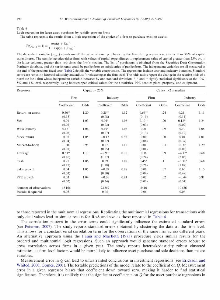
Table 6 presents the results of a logit regression on firms’ engaging in large asset purchases during periods ofrapid growth. The rapid growth columns in Panel A of Table 1 present the results of a similar analysis on thesimulated data set. The standard errors in parentheses adjust for heteroskedasticity and clustering at the firmlevel. Statistical significance is inferred using bootstrapped critical values for the t-statistics. As with thesimulated data, firms with higher RoA engage in large asset purchases during periods of rapid growth. Theodds ratios indicate an economically meaningful impact of RoA on the asset purchase decision. While most ofthe control variables have little impact, low industry leverage values encourage asset purchases. These findingssupport the model’s prediction that firms with higher profitability seek external growth.
Hypothesis 2 links the level of asset purchases to the firm’s investment opportunities. Table 7 presents theresults of testing this relation for firms with large asset purchases, conditional on a period of rapid growth. Therapid growth columns in Panel C of Table 1 report the simulation counterpart to this analysis. The selectionequation uses the same controls as in the logit regressions. Statistical significance is inferred usingbootstrapped critical values for the t-statistics.
The results demonstrate that, as predicted by the model, transaction size covaries with the firm’s Q for largeasset purchases. The macro Q regressions yield consistently higher point estimates and lower p-values thanfinance Q regressions. Further, cash flow is not significant in any of these specifications. Whereas the inverseMill’s ratio is not significant using the bootstrapped critical values, it is asymptotically significant in many ofthe regressions. Thus, conditional on a decision to engage in a large asset purchase, the transaction sizeincreases with the firm’s growth opportunities.
5.5. Robustness
The panel nature of the sample provides some challenges to the statistical analysis. A fixed-effects logitregression estimates a binary logit model for asset purchases only on the subsample of firms that eitherpurchased or sold assets in at least one year. This allows for a firm-level fixed effect in the estimation. Theestimation of fixed-effects logit models for asset purchases and sales generate similar results for RoA and size
12I thank the referee for suggesting this analysis.
ARTICLE IN PRESS
Table 6
Logit regression for large asset purchases by rapidly growing firms
The table represents the results from a logit regression of the choice of a firm to purchase existing assets:
Prðyi;tþ1 ¼ 1Þ ¼expðat þ bxi;tÞ
1þ expðat þ bxi;tÞ.
The dependent variable ðyi;tþ1Þ equals one if the value of asset purchases by the firm during a year was greater than 50% of capital
expenditures. The sample includes either firms with values of capital expenditures to replacement value of capital greater than 25% or, in
the latter columns, greater than two times the firm’s median. The list of purchasers is obtained from the Securities Data Corporation
Platinum database, and the participants could be public firms or subsidiaries of public firms. The independent variables are all measured at
the end of the previous fiscal year. Table 2 details the variable construction. The regressions include year and industry dummies. Standard
errors are robust to heteroskedasticity and adjust for clustering at the firm level. The odds ratios report the change in the relative odds of a
purchase for a firm whose independent variable increases by one standard deviation, þ, � and �� signify statistical significance at the 10%,
5% and 1% level, respectively, using bootstrapped critical values for the t-statistics. PPE denotes plant, property, and equipment.
Regressor Capex 4 25% Capex 42�median
Firm Industry Firm Industry
Coefficient Odds Coefficient Odds Coefficient Odds Coefficient Odds
Return on assets 0.56�� 1.20 0.25�� 1.12 0.64�� 1.24 0.21þ 1.11
(0.13) (0.08) (0.19) (0.11)
Size 0.01 1.03 0.04� 1.08 0.10�� 1.20 0.12�� 1.24
(0.02) (0.02) (0.03) (0.02)
Wave dummy 0.13þ 1.06 0.19� 1.08 0.21 1.09 0.10 1.05
(0.08) (0.07) (0.13) (0.12)
Stock return 0.07 1.05 �0.13 0.98 0.00 1.00 0.04 1.01
(0.04) (0.22) (0.06) (0.37)
Market-to-book �0.00 0.98 0.07 1.10 0.01 1.03 0.18� 1.29
(0.01) (0.05) (0.01) (0.08)
Leverage 0.53�� 1.13 �2.93� 0.76 0.36 1.09 �4.17� 0.68
(0.16) (1.37) (0.24) (2.06)
Cash 0.27 1.06 0.69 1.08 0.45þ 1.11 �3.30þ 0.68
(0.17) (1.28) (0.26) (1.87)
Sales growth 0.04 1.05 �0.09 0.98 0.06 1.07 0.65 1.15
(0.03) (0.30) (0.04) (0.47)
PPE growth 0.03 1.04 �0.26 0.94 0.02 1.02 �0.44 0.91
(0.02) (0.24) (0.03) (0.34)
Number of observations 18 166 22 352 8416 10 636
Pseudo R-squared 0.05 0.05 0.06 0.06
M. Warusawitharana / Journal of Financial Economics 87 (2008) 471–497490
to those reported in the multinomial regressions. Replicating the multinomial regressions for transactions withonly deal values lead to similar results for RoA and size as those reported in Table 4.
The correlation pattern in the error terms could significantly influence the estimated standard errors(see Petersen, 2007). The study reports standard errors obtained by clustering the data at the firm level.This allows for a constant serial correlation term for the observations of the same firm across different years.An alternative approach using the Fama and MacBeth (1973) procedure yields similar results for theordered and multinomial logit regressions. Such an approach would generate standard errors robust tocross correlation across firms in a given year. The study reports heteroskedasticity robust clusteredestimates, as firm-level factors would be more likely to influence asset purchase and sale decisions than macrovariables.
Measurement error in Q can lead to unwarranted conclusions in investment regressions (see Erickson andWhited, 2000; Gomes, 2001). The testable predictions of the model relate to the coefficient on Q. Measurementerror in a given regressor biases that coefficient down toward zero, making it harder to find statisticalsignificance. Therefore, it is unlikely that the significant coefficients on Q for the asset purchase regressions in

ARTICLE IN PRESS
Table 7
Investment regression for large asset purchases by rapidly growing firms
The table reports the results from estimating the following equation:
I
K¼ cþ a �Qþ b � CF þ �,
conditional on the firm purchasing existing assets worth greater than 50% of capital expenditures, where I denotes the value of the assets
purchased, Q measures either finance Q or macro Q, and CF equals cash flow. The scaling variable K equals book assets for the finance Q
regression and the replacement value of capital for the macro Q regression. The sample includes either firms with values of capital
expenditures to replacement value of capital greater than 25% or, in Panel B, greater than two times the firm’s median. The resulting
model is estimated using a Heckman two-step estimator. The selection equation includes size, return on assets, market-to-book, wave
dummy, stock return, leverage, cash, sales growth, and PPE (plant, property, and equipment) growth as independent variables. The
industry columns present results with the control variables for the selection equation replaced by their industry means. The selection
equation and the investment equation include year and industry dummies. The sample of asset purchases is obtained from the Securities
Data Corporation Platinum database and ranges from 1985 to the end of 2005. The tables report the number of uncensored observations,� and �� signify statistical significance at the 5% and 1% level, respectively, using bootstrapped critical values for the t-statistics.
Regressor Finance Q Macro Q
Firm Industry Firm Industry
Panel A: Large asset purchases by firms with capex 425%
Tobin’s Q 0.009� 0.008� 0.013� 0.015��
(0.003) (0.003) (0.005) (0.005)
Cash flow 0.051 0.036 0.020 0.023
(0.030) (0.023) (0.034) (0.033)
Inverse Mill’s ratio 0.298 0.445 0.567 0.729
(0.093) (0.108) (0.276) (0.261)
Number of observations 1198 1475 720 836
Adjusted R-squared 0.06 0.06 0.02 0.03
Panel B: Large asset purchases by firms with capex 42�median
Tobin’s Q 0.012� 0.011� 0.035�� 0.027��
(0.005) (0.004) (0.009) (0.008)
Cash flow 0.083 0.018 0.050 0.029
(0.046) (0.027) (0.062) (0.053)
Inverse Mill’s ratio 0.241 0.138 0.663 0.502
(0.099) (0.082) (0.328) (0.285)
Number of observations 468 573 298 344
Adjusted R-squared 0.12 0.11 0.04 0.03
M. Warusawitharana / Journal of Financial Economics 87 (2008) 471–497 491
Tables 5 and 7 are driven by measurement errors in Q. In the absence of measurement error, the true pointestimates would be greater than those reported in Tables 5 and 7.
Measurement error in Q also affects inference on the cash flow coefficient. The proxy quality thresholdmethod of Erickson and Whited (2005) computes the minimum correlation between observed and true Q
required to infer positivity of another coefficient under various assumptions on the measurement errorstructure. A high threshold value implies that the observed Q must be a good proxy for the true Q for thecoefficient sign of interest to be robust to measurement error. The reverse regression of Q on investment, cashflow, and the inverse Mill’s ratio for asset purchases yields positive cash flow coefficients with the finance Q
and negative coefficients with the macro Q. This indicates that, using the finance Q as the proxy for true Q, thecash flow coefficient is positive under the classical errors-in-variables model and when the measurement erroris correlated with one or more of the regressors but not the disturbance. Proxy quality computation usingmacro Q leads to thresholds around 0.20 under the above assumptions. Under the assumption that themeasurement error correlates with the disturbance but not the regressors, the threshold increases to 0.50 forthe macro Q. This implies that the correlation between macro Q and the true incentive to invest must begreater than 0.50 for the positive cash flow coefficient to be robust to measurement error. Whereas the positive

ARTICLE IN PRESS
Table 8
Multinomial logit regression for asset transactions with free cash flow
The table represents the results from a multinomial logit regression of the choice of a firm to purchase or sell existing assets:
Prðyi;tþ1 ¼ jÞ ¼expðat þ bjxi;tÞ
1þ expðat þ bjxi;tÞ.
The dependent variable ðyi;tþ1Þ takes three values depending on whether the firm or a subsidiary bought existing assets, sold existing assets,
or did neither. The table reports the coefficients for purchasing or selling assets compared with doing neither. The list of purchasers and
sellers is obtained from the Securities Data Corporation Platinum database, and the participants may be public firms or subsidiaries of
public firms. The sample consists of all firms listed on Compustat from 1984 to 2004 that contain information on the independent
variables. The independent variables are all measured at the end of the previous fiscal year. Free cash flow equals operating cash flow net
of investment activity and is obtained from the statement of cash flows. Table 2 details the construction of other variables. The regressions
include year and industry dummies. Standard errors are robust to heteroskedasticity and adjust for clustering at the firm level. The odds
ratios report the change in the relative odds of a purchase or a sale for a firm whose independent variable increases by one standard
deviation, � and �� signify statistical significance at the 5% and 1% level, respectively, using bootstrapped critical values for the t-statistics.
PPE denotes plant, property, and equipment.
Regressor Purchase Sale
Coefficient Odds ratio Coefficient Odds ratio
Free cash flow �0.05 0.98 �0.28�� 0.89
(0.03) (0.07)
Size 0.26�� 1.75 0.38�� 2.27
(0.01) (0.01)
Wave dummy 0.11�� 1.05 �0.05 0.98
(0.03) (0.05)
Stock return 0.14�� 1.10 �0.20�� 0.88
(0.02) (0.04)
Market-to-book 0.02�� 1.08 0.02�� 1.07
(0.003) (0.004)
Leverage �0.35�� 0.92 0.51�� 1.14
(0.07) (0.10)
Cash �0.48�� 0.91 �1.32�� 0.76
(0.09) (0.16)
Sales growth 0.09�� 1.08 �0.18�� 0.86
(0.01) (0.06)
PPE growth 0.06�� 1.05 �0.18�� 0.86
(0.01) (0.06)
Number of observations 74 227 74 227
Pseudo R-squared 0.07 0.07
M. Warusawitharana / Journal of Financial Economics 87 (2008) 471–497492
cash flow coefficients in Table 5 match the simulation results, these computations demonstrate that inferenceon the cash flow coefficients is sensitive to measurement error in Q (see Erickson and Whited, 2000).
The significant and positive coefficient on RoA can be interpreted in favor of an alternative hypothesisbased on agency conflicts. The agency hypothesis argues that managers derive benefits from increased size anduse free cash flow to grow via asset purchases. High return on assets indicates increased cash flow to the firm,and managers with misaligned incentives use the excess cash to grow the firm and increase their privatebenefits. Proposition 4 demonstrates that value-maximizing managers respond to increased profitability byengaging in asset purchases. The replication of the above logit regressions with a free cash flow measureprovides a test of the alternative hypothesis. The free cash flow variable measures net operating cash flowminus cash flow for investing activities, divided by book assets at the beginning of the fiscal year.13
13Net operating cash flow and net investing cash flow are given by Compustat variables 308 and 311, respectively. Free cash flow ¼
data308 + data311. Free cash flow measures the cash generated from operations net of investment activity. These variables are available
from 1987 onward.

ARTICLE IN PRESSM. Warusawitharana / Journal of Financial Economics 87 (2008) 471–497 493
Table 8 presents the results of estimating the multinomial logit regression using free cash flow in place of RoA.The coefficient on free cash flow itself is statistically insignificant as a predictor of asset purchases and significantlynegative as a predictor of asset sales. This provides evidence that high free cash flow does not lead to assetpurchases and indicates that the impact of RoA on asset purchases does not capture a free cash flow effect. Thesefindings demonstrate that one can reject the alternative hypothesis on asset purchases based on agency arguments.Overall, the empirical evidence supports the two efficiency-based hypotheses on asset purchases and sales.
6. Conclusion
The study argues that decisions over the optimal scale of the firm drive organic investment, acquisitions, andasset sales. The paper analyzes these transactions in the context of an efficiency-based model: Asset purchasesand sales help firms move toward their optimal size after heterogenous productivity shocks. Conditional on afirm buying or selling existing assets, the model links purchases and sales of existing assets to the marginalvalue of capital inside the firm. The profitability and size of the firm determines whether the firm chooses tobuy or sell existing assets.
The paper tests the implications of the model using a data set of asset purchases and sales from the SDCPlatinum database. The estimation of the selection models for investment demonstrates a positive link betweenthe quantity of assets purchased and the investment opportunities of the firm. Return on assets and sizestrongly predict the likelihood of a firm engaging in an asset purchase or sale. A unit standard deviationincrease in RoA increases the probability of an asset purchase by 29%, while a corresponding decrease in RoAincreases the likelihood of an asset sale by 34%. Focusing the analysis on large asset purchases by firms duringperiods of rapid growth yields similar results. The empirical analysis also finds that financing considerationsinfluence the decision of firms to sell assets, with lower levels of liquid assets leading to more asset sales.However, increased cash stocks do not lead to increased asset purchases, indicating that empire-buildingtendencies do not influence asset purchases.
The findings on asset purchases contrast with the evidence linking agency problems and misvaluations tomergers. Further research on the sources and effects of the differences between mergers and asset purchasescould prove fruitful, given that the fundamental action of both transactions is to shift ownership of someproductive assets from one firm to another.
Appendix A. Proofs
Proposition 1. There exists a threshold ~I ¼ a1�p
h i1=ð1�yÞbelow which all investment consists of new investment and
above which all investment consists of purchased existing capital:
I ¼ N if 0pIp ~I
I ¼M if Io0 or I4 ~I .
Corollary 1. The investment cost function CnðI ;KÞ obtained by substitution of the above allocation choice is
continuous.
Proof. The differentiation of Eq. (6) yields the first-order conditions for optimality:
qC
qN¼ 1þ
qFðI ;KÞqI
and
qC
qM¼ pþ
qFðI ;KÞqI
þ ayMy�1 � 1ðM40Þ. ð19Þ
There does not exist an interior solution to the problem. The boundary conditions imply that
Cð ~I ; 0;KÞ ¼ Cð0; ~I ;KÞ. (20)
The solution to the above equation yields that ~I ¼ a1�p
h i1=ð1�yÞ. As asset purchases have a lower marginal cost
of investment for IX ~I , ðpþ ð1� pÞyo1Þ, the firm buys assets. The transaction cost of asset purchases CðMÞ
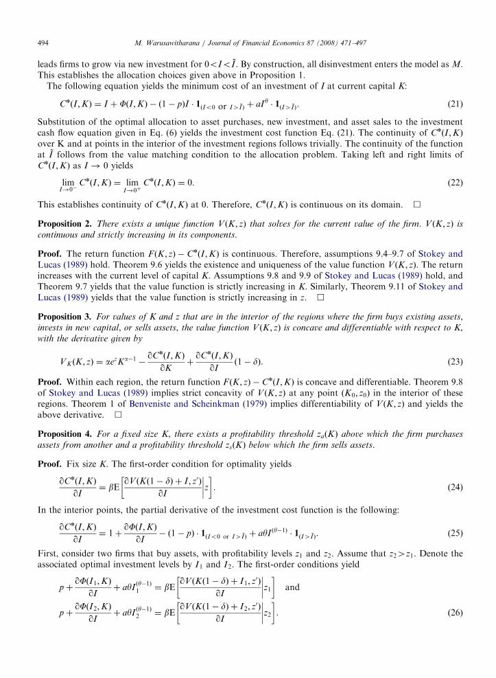
ARTICLE IN PRESSM. Warusawitharana / Journal of Financial Economics 87 (2008) 471–497494
leads firms to grow via new investment for 0oIo ~I . By construction, all disinvestment enters the model as M.This establishes the allocation choices given above in Proposition 1.
The following equation yields the minimum cost of an investment of I at current capital K:
CnðI ;KÞ ¼ I þ FðI ;KÞ � ð1� pÞI � 1ðIo0 or I4 ~IÞ þ aIy � 1ðI4 ~IÞ. (21)
Substitution of the optimal allocation to asset purchases, new investment, and asset sales to the investmentcash flow equation given in Eq. (6) yields the investment cost function Eq. (21). The continuity of CnðI ;KÞover K and at points in the interior of the investment regions follows trivially. The continuity of the functionat ~I follows from the value matching condition to the allocation problem. Taking left and right limits ofCnðI ;KÞ as I ! 0 yields
limI!0�
CnðI ;KÞ ¼ limI!0þ
CnðI ;KÞ ¼ 0. (22)
This establishes continuity of CnðI ;KÞ at 0. Therefore, CnðI ;KÞ is continuous on its domain. &
Proposition 2. There exists a unique function V ðK ; zÞ that solves for the current value of the firm. V ðK ; zÞ is
continuous and strictly increasing in its components.
Proof. The return function F ðK ; zÞ � CnðI ;KÞ is continuous. Therefore, assumptions 9.4–9.7 of Stokey andLucas (1989) hold. Theorem 9.6 yields the existence and uniqueness of the value function V ðK ; zÞ. The returnincreases with the current level of capital K. Assumptions 9.8 and 9.9 of Stokey and Lucas (1989) hold, andTheorem 9.7 yields that the value function is strictly increasing in K. Similarly, Theorem 9.11 of Stokey andLucas (1989) yields that the value function is strictly increasing in z. &
Proposition 3. For values of K and z that are in the interior of the regions where the firm buys existing assets,invests in new capital, or sells assets, the value function V ðK ; zÞ is concave and differentiable with respect to K,with the derivative given by
VK ðK ; zÞ ¼ aezKa�1 �qCnðI ;KÞ
qKþ
qCnðI ;KÞ
qIð1� dÞ. (23)
Proof. Within each region, the return function F ðK ; zÞ � CnðI ;KÞ is concave and differentiable. Theorem 9.8of Stokey and Lucas (1989) implies strict concavity of V ðK ; zÞ at any point ðK0; z0Þ in the interior of theseregions. Theorem 1 of Benveniste and Scheinkman (1979) implies differentiability of V ðK ; zÞ and yields theabove derivative. &
Proposition 4. For a fixed size K, there exists a profitability threshold zaðKÞ above which the firm purchases
assets from another and a profitability threshold zsðKÞ below which the firm sells assets.
Proof. Fix size K. The first-order condition for optimality yields
qCnðI ;KÞ
qI¼ bE
qV ðKð1� dÞ þ I ; z0Þ
qI
� ����z�. (24)
In the interior points, the partial derivative of the investment cost function is the following:
qCnðI ;KÞ
qI¼ 1þ
qFðI ;KÞqI
� ð1� pÞ � 1ðIo0 or I4 ~IÞ þ ayI ðy�1Þ � 1ðI4 ~IÞ. (25)
First, consider two firms that buy assets, with profitability levels z1 and z2. Assume that z24z1. Denote theassociated optimal investment levels by I1 and I2. The first-order conditions yield
pþqFðI1;KÞ
qIþ ayI
ðy�1Þ1 ¼ bE
qV ðKð1� dÞ þ I1; z0Þ
qI
� ����z1�
and
pþqFðI2;KÞ
qIþ ayI
ðy�1Þ2 ¼ bE
qV ðKð1� dÞ þ I2; z0Þ
qI
� ����z2�. ð26Þ

ARTICLE IN PRESSM. Warusawitharana / Journal of Financial Economics 87 (2008) 471–497 495
Monotonicity of the transition function for z implies that
EqV ðKð1� dÞ þ I2; z0Þ
qI
� ����z2�4E
qV ðKð1� dÞ þ I2; z0Þ
qI
� ����z1�. (27)
Substituting the first-order conditions to the above inequality yields
EqV ðKð1� dÞ þ I1; z0Þ
qI
� ����z1��
qFðI1;KÞqI
� ayIy�11
4EqV ðKð1� dÞ þ I2; z0Þ
qI
� ����z1��
qFðI2;KÞqI
� ayIy�12 . ð28Þ
A proof by contradiction establishes that I24I1. Assume that I2pI1. Then, concavity of the value functionand convexity of the adjustment cost function imply the following inequality:
EqV ðKð1� dÞ þ I1; z0Þ
qI
����z1� �
�qFðI1;KÞ
qI� ayIy�11
pEqV ðKð1� dÞ þ I2; z0Þ
qI
����z1� �
�qFðI2;KÞ
qI� ayIy�12 . ð29Þ
This contradicts Eq. (28). Therefore I24I1. The proof requires a low marginal transaction cost (ao lKyð1�yÞ
when qFðI ;KÞqI¼ lI
K).
A similar proof establishes that for two firms, both of which either sell assets or invest in new capital, thefirm with higher profitability invests more ðz24z1 ) I24I1Þ. Investment increases monotonically with z, anda firm buys assets if I4 ~I and sells assets when Io0. This establishes the proposition. &
Proposition 5. For a given level of profitability z, there exists a size threshold KsðzÞ above which the firm sells
assets.
Proof. Fix profitability z. Consider a firm with capital K1 that optimally engages in asset sales and anotherfirm with capital K24K1. The result requires that I2o0. Assuming that these are in the interior of the actionregions, the first-order conditions imply
pþqFðI1;K1Þ
qI¼ bE
qV ðK1ð1� dÞ þ I1; z0Þ
qI
� ����z�
and
pþqFðI2;K2Þ
qIpbE
qV ðK2ð1� dÞ þ I2; z0Þ
qI
� ����z�. ð30Þ
The constant returns to scale assumption implies that qFðI ;KÞqI
is an increasing function of IK. A proof by
contradiction establishes that I2o0. Assume that I2X0. Therefore I1K1
p I2K2. This implies that
qFðI1;K1Þ
qIp
qFðI2;K2Þ
qI. (31)
Substituting the above into the first-order conditions given in Eq. (30) yields
EqV ðK1ð1� dÞ þ I1; z0Þ
qI
� ����z�pE
qV ðK2ð1� dÞ þ I2; z0Þ
qI
� ����z�. (32)
The concavity of the value function implies that
K1ð1� dÞ þ I1XK2ð1� dÞ þ I2,
) I1XðK2 � K1Þð1� dÞ þ I2. ð33Þ
Therefore I1X0. This contradicts the initial assumption of an asset sale. &

ARTICLE IN PRESSM. Warusawitharana / Journal of Financial Economics 87 (2008) 471–497496
Appendix B. Numerical solution
The numerical solution employs value function iteration over a grid of values for current capital,investment, and profitability. The capital grid consists of five hundred equally spaced points, while theinvestment grid contains five thousand points. The Tauchen and Hussey (1991) approximation for AR(1)processes yields the grid of values for profitability. This grid contains ten points. The solution uses theoptimal allocation choices derived as the solution to Eq. (11). The solution yields an optimal policy for newinvestment, asset purchases, and asset sales. For a given level of capital, the transaction costs of assetpurchases lead to an upper and lower bound for profitability beyond which the firm buys and sells assets,respectively. These bounds follow a smooth function as K varies. The acquisition boundary for a given capitallevel is approximated by the interpolated value of z, which yields an optimal total investment of ~I . Themidpoint of the profitability levels over which the firm begins to disinvest yields the approximate salethreshold. These values act as inputs to a polynomial approximation of the acquire and sell thresholds as afunction of logðKÞ. The solution uses a second-order approximation with Hermite polynomials. Within eachaction region, linear interpolation provides the investment decisions and firm values.
Appendix C. Simulations
The simulations apply the policy functions derived above to a panel of firms. The simulated sample consistsof one thousand firms over one hundred time periods. The simulation employs the boundaries for assetpurchases and sales obtained in the numerical solution. The initial 20 periods function as a burn-in sample.The sequence of solutions to the value function and simulation iterates until the equilibrium value of p atwhich total demand for asset purchases equals total asset sales is obtained. This corresponds to the steadystate of the economy, in which the interfirm assets market clears. Hopenhayn (1992) provides the theoreticalfoundation for this approach.
References
Abel, A., 1983. Optimal investment under uncertainty. American Economic Review 73, 228–233.
Abel, A., Eberly, J.C., 1994. A unified model of investment under uncertainty. American Economic Review 84, 1369–1384.
Alexander, G.J., Bensen, G.P., Kampmeyer, J.M., 1984. Investigating the valuation effects of announcements of voluntary corporate
selloffs. Journal of Finance 39, 502–517.
Andrade, G., Mitchell, M., Stafford, E., 2001. New evidence and perspectives on mergers. Journal of Economic Perspectives 15, 103–120.
Bates, T.W., 2005. Asset sales, investment opportunities, and the use of proceeds. Journal of Finance 60, 105–135.
Benveniste, L.M., Scheinkman, J.A., 1979. On the differentiability of the value function in dynamic models of economics. Econometrica
47, 727–732.
Bruner, R.F., 2004. Applied Mergers and Acquisitions. Wiley, New Jersey.
Caballero, R.J., Engel, E.M.R.A., 1999. Explaining investment dynamics in US manufacturing: a generalized (S,s) approach.
Econometrica 67, 783–826.
Colak, G., Whited, T.M., 2007. Spin-offs, divestitures and conglomerate investment. Review of Financial Studies 20, 557–595.
Cooper, R.W., Ejarque, J., 2003. Financial frictions and investment: requiem in q. Review of Economic Dynamics 6, 710–728.
Cooper, R.W., Haltiwanger, J., 2006. On the nature of capital adjustment costs. Review of Economic Studies 73, 611–633.
Dong, M., Hirshleifer, D., Richardson, S., Teoh, S.H., 2006. Does investor misvaluation drive the takeover market? Journal of Finance 61,
725–762.
Efron, B., Tibshirani, R., 1993. An Introduction to the Bootstrap. Chapman & Hall, New York.
Eisfeldt, A.L., Rampini, A., 2006. Capital reallocation and liquidity. Journal of Monetary Economics 53, 369–399.
Eisfeldt, A.L., Rampini, A., 2007. New or used? investment with credit constraints. Journal of Monetary Economics, forthcoming.
Erickson, T., Whited, T.M., 2000. Measurement error and the relationship between investment and q. Journal of Political Economy 108,
1027–1057.
Erickson, T., Whited, T.M., 2005. Proxy-quality thresholds: theory and applications. Financial Research Letters 2, 131–151.
Erickson, T., Whited, T.M., 2006. On the accuracy of different measures of q. Financial Management 35, 5–33.
Fama, E.F., MacBeth, J.D., 1973. Risk, return, and equilibrium: empirical tests. Journal of Political Economy 81, 607–636.
Fazzari, S.M., Hubbard, R.G., Petersen, B.C., 1988. Financing constraints and corporate investment. Brookings Papers on Economic
Activity 1, 141–195.
Gomes, J., Livdan, D., 2004. Optimal diversification: reconciling theory and evidence. Journal of Finance 59, 507–535.
Gomes, J.F., 2001. Financing investment. American Economic Review 90, 1263–1285.

ARTICLE IN PRESSM. Warusawitharana / Journal of Financial Economics 87 (2008) 471–497 497
Grossman, S.J., Hart, O.D., 1986. The costs and benefits of ownership: a theory of vertical and lateral integration. Journal of Political
Economy 94, 691–719.
Hall, R.E., 2004. Measuring factor adjustment costs. Quarterly Journal of Economics 119, 899–927.
Harford, J., 2005. What drives merger waves? Journal of Financial Economics 77, 529–560.
Hart, O.D., Moore, J., 1990. Property rights and the nature of the firm. Journal of Political Economy 98, 1119–1158.
Hayashi, F., 1982. Tobin’s marginal q and average q: a neoclassical interpretation. Econometrica 50, 213–224.
Heckman, J.J., 1974. Shadow prices market, wages, and labor supply. Econometrica 42, 679–694.
Hennessy, C.A., Whited, T.M., 2005. Debt dynamics. Journal of Finance 60, 1129–1165.
Hennessy, C.A., Levy, A., Whited, T.M., 2007. Testing q theory with financing frictions. Journal of Financial Economics 83, 691–717.
Hite, G.L., Owers, J.E., Rogers, R.C., 1987. The market for interfirm asset sales. Journal of Financial Economics 18, 229–253.
Hopenhayn, H.A., 1992. Entry, exit, and firm dynamics in long run equilibrium. Econometrica 60, 1127–1150.
Hovakimian, G., Titman, S., 2006. Corporate investment with financial constraints: sensitivity of investment to funds from voluntary asset
sales. Journal of Money, Credit, and Banking 38, 357–374.
Jain, P.C., 1985. The effect of voluntary sell-off announcements on shareholder wealth. Journal of Finance 40, 209–223.
John, K., Ofek, E., 1995. Asset sales and increase in focus. Journal of Financial Economics 37, 105–126.
Jovanovic, B., Rousseau, P., 2002. The q-theory of mergers. American Economic Association (Papers and Proceedings) 92, 198–204.
Klein, B., Crawford, R.G., Alchian, A.A., 1978. Vertical integration, appropriable rents, and the competitive contracting process. Journal
of Law and Economics 21, 297–326.
Lang, L.H.P., Poulson, A.B., Stulz, R.M., 1995. Asset sales firm performance and the agency costs of managerial discretion. Journal of
Financial Economics 37, 3–37.
Ljungqvist, A., Wilhelm Jr., W.J., 2003. Ipo pricing in the dot-com bubble. Journal of Finance 58, 723–752.
Loughran, T., Vijh, A., 1997. Do long-term shareholders benefit from corporate acquisitions? Journal of Finance 52, 1765–1790.
Lucas Jr., R.E., 1967. Adjustment costs and the theory of supply. Journal of Political Economy 75, 321–334.
Maksimovic, V., Phillips, G., 2001. The market for corporate assets: who engages in mergers and asset sales and are there efficiency gains?
Journal of Finance 56, 2019–2065.
Maksimovic, V., Phillips, G., 2002. Do conglomerates allocate resources efficiently? Journal of Finance 57, 721–767.
Moeller, S.B., Schlingemann, F.P., Stulz, R.M., 2005. Wealth destruction on a massive scale? A study of acquiring-firm returns in the
recent merger wave. Journal of Finance 60, 757–782.
Petersen, M.A., 2007. Estimating standard errors in finance panel data sets: comparing approaches. Review of Financial Studies,
forthcoming.
Pulvino, T.C., 1998. Do asset fire sales exist? An empirical investigation of commercial aircraft transactions. Journal of Finance 53,
939–978.
Ramey, V.A., Shapiro, M.D., 2001. Displaced capital: a study of aerospace plant closings. Journal of Political Economy 109, 958–992.
Ray, S., Warusawitharana, M., 2007. An efficiency perspective on the gains from mergers and asset purchases. Unpublished working
paper. Board of Governors of the Federal Reserve System, Washington, DC.
Rhodes-Kropf, M., Robinson, D.T., Viswanathan, S., 2005. Valuation waves and merger activity: the empirical evidence. Journal of
Financial Economics 77, 561–603.
Salinger, M.A., Summers, L.H., 1983. Tax reform and corporate investment: a microeconometric simulation study. In: Feldstein, M.
(Ed.), Behavioral Simulation Methods in Tax Policy Analysis. University of Chicago Press, Chicago, IL.
Schlingemann, F.P., Stulz, R.M., Walkling, R.A., 2002. Divestitures and the liquidity of the market for corporate assets. Journal of
Financial Economics 64, 117–144.
Schoar, A., 2002. Effects of corporate diversification on productivity. Journal of Finance 57, 2379–2403.
Slovin, M.B., Sushka, M.E., Poloncheck, J.A., 2005. Methods of payment in asset sales: contracting with equity versus cash. Journal of
Finance 60, 2385–2407.
Stokey, N.L., Lucas Jr., R.E., 1989. Recursive Methods in Economic Dynamics. Harvard University Press, Cambridge, MA.
Tauchen, G., Hussey, R., 1991. Quadrature-based methods for obtaining approximate solutions to nonlinear asset pricing models.
Econometrica 59, 371–396.
Whited, T.M., 1992. Debt, liquidity constraints, and corporate investment: evidence from panel data. Journal of Finance 47, 1425–1460.
Whited, T.M., 2006. External finance constraints and the intertemporal pattern of intermittent investment. Journal of Financial
Economics 81, 467–502.
Williamson, O.E., 1975. Markets and Hierarchies: Analysis and Antitrust Implications. Free Press, New York.
Yang, L., 2006. The real determinants of asset sales. Unpublished working paper. University of California, Los Angeles.