corporate default prediction with financial ratios and macroeconomic variables

Corporate Default Prediction with Financial Ratios andMacroeconomic Variables

Economics

Master's thesis

Tomi Stenbäck

2013

Department of EconomicsAalto UniversitySchool of Business

Powered by TCPDF (www.tcpdf.org)

http://lib.aalto.fi

http://www.tcpdf.org

1

Abstract

In this master thesis paper I study corporate default prediction with firm specific financial

ratios and macroeconomic variables. I show how regressions default prediction ability

increases when macroeconomic variables are added into the model of financial ratios. In

analysis I have financial ratio data from period 1999 to 2011 from industries of construction

and retail including 35000 firms and over 200000 observations. The data is from Suomen

Asiakastieto, Tilastokeskus and Suomen Pankki. In measuring the goodness of the models I

use different analysis of the predicted values like five levels risk classification. This risk

classification can also be thought as credit rating.

Keywords: default prediction, credit rating, risk classification

2

Table of Contents

Sisällysluettelo

Abstract ................................................................................................................................... 1

Table of Contents........................................................................................................................ 2

1. Introduction ......................................................................................................................... 4

1.1. Progress of the study in this paper ................................................................................... 5

2. Credit Rating Industry ......................................................................................................... 6

3. Science and models ............................................................................................................. 7

3.1. The use of financial information before 1960 ................................................................. 7

3.2. Single financial ratios as predictors ............................................................................... 10

3.3. Multiple variable models ............................................................................................... 12

3.4. The use of background information in prediction ......................................................... 13

3.5. Models and macroeconomic .......................................................................................... 14

4. Hypothesis ......................................................................................................................... 16

5. Econometric Research ....................................................................................................... 16

5.1. Data ................................................................................................................................ 17

5.2. Variables ........................................................................................................................ 18

5.2.1. Dependent variable ................................................................................................. 18

5.2.2. Macroeconomic explanatory variables ................................................................... 19

5.3. Working with data ......................................................................................................... 20

5.3.1. Cleaning financial ratio data .................................................................................. 21

5.3.2. Defaulted firms by industry .................................................................................... 22

5.3.3. Descriptive statistics of ratios ................................................................................ 22

5.3.4. Descriptive statistics of macroeconomic variables ................................................ 24

5.4. Regression models ......................................................................................................... 27

5.4.1. The linear probability model .................................................................................. 27

3

5.4.2. The logit model ...................................................................................................... 28

5.5. Regressions .................................................................................................................... 28

5.5.1. Testing industry variables ...................................................................................... 29

5.5.2. Defining the goodness of a regression model ........................................................ 30

5.5.3. Linear regression with financial ratios only ........................................................... 33

5.5.4. Regression with already occurred default and growth variable added ................... 34

5.5.5. Regression with macroeconomic variables ............................................................ 35

5.5.6. Results of regression B with macroeconomic variables added one by one ........... 40

5.5.7. Result of regression models A, B and C ................................................................ 43

5.5.8. Correlation between variables ................................................................................ 47

6. Testing regression model to test data ................................................................................ 48

7. Results to hypothesis ......................................................................................................... 49

8. Conclusions ....................................................................................................................... 50

References ................................................................................................................................ 51

Appendices ............................................................................................................................... 53

4

1. Introduction

The default prediction of firms is a widely studied issue. When banks and other financial

institutions are giving loans to firms they have to value the risk of those firms. This is where

the Credit Rating industry is giving their contribution. Credit Rating institutions are

measuring the firms’ characteristics from the different data that is available. From these

characteristics the firms are rated by their risk and are given a credit rating which tells how

probable is it that the firm is having payment difficulties or even go to bankruptcy in the near

future. Different Credit Rating industries are using slightly different kind of methods how

they value the firms and how the rating is written. For example in United States a Credit

Rating institution Standard and Poor’s is using 21 level ratings from the lowest speculative

grade D to the highest investment grade AAA (Cantor & Packer 2006).

In predicting the default of firms, the most used and most important information is coming

from the firms’ historical data, which contains ratios from the financial statements,

information of the firms’ previous payment difficulties and information of the management’s

possible payment difficulties from other firms they are related. Size and age of firm as well as

Personal marks of failure in payment behavior also give some information. An example, of

default prediction based only on financial statement ratios, is widely referred Edward I.

Altman’s Z-score. In Z-score model there are five financial statement explanatory variables

with different weights, which are giving the Z-score value. The Z-score value is explaining

the probability of the firm’s default in the near future (Altman 1968).

Even that the issue is widely studied, the models and research is mostly based on firm specific

financial statement data. The reason for this might be that firm specific models are already

giving very good predictions of the future risks. And if the model is already good enough it

might be better to keep it also simple as possible. The simplicity makes it more transparent

and easier to use and sell to customers. What I find the problem here is that the firm specific

financial information is, firstly historical and secondly does not tell anything about the

macroeconomic conditions at certain time. An economic shock can bring huge risks in

businesses, but we can’t see these risks, if just look to the historical firm specific information.

My contribution is that I’m trying to find new variables from macroeconomic data to improve

the ability to predict the probability of default. These “new” macroeconomic variables are

industry volumes, gross national income, interest rate, consumption and consumer confidence

5

on the economy. One reasons why I think the macroeconomic variables could give new value

to the firm specific models, is that the financial statement information on small firms is

historical information and is approximately 18 months old (Asiakastieto), when the

macroeconomic data of quarterly macroeconomic accountancy is instead 6 to 9 months old

(Tilastokeskus). So if there is an economic shock like sudden financial crisis, the 18 month

old firm specific historical data could give a view that everything is fine, but when we are

looking the industry index or other macroeconomic conditions, we might see that this is

probably not the case.

For analysis I’m using firm specific financial ratio data from Suomen Asiakastieto and

macroeconomic data from Tilastokeskus and Suomen Pankki. I’m studying two different

industries which are construction and retail.

The firm specific variables are gearing ratio, quick ratio, return on investment and logarithm

of net sales.

The macroeconomic variables are industry index or volume, interest rate, consumption, gross

national income and consumer confidence on economy,

The null hypothesis H0 is that the new macroeconomic variables are not giving any new value

to the existing firm specific models. My ambition is to attack against the null hypothesis and

try to reject it. My other hypothesis H1, H2 and H3 are:

H1: The macro level variables are significant in the regression model with financial ratios and

macroeconomic variables when the dependent variable is default of a firm.

H2: The macro level variables improve the model’s ability to predict future defaults.

H3: The newer the macroeconomic data used in model, the more significant the macro

variables are and better it predicts the future defaults.

1.1. Progress of the study in this paper

In section 2 I start with explaining few words about credit rating industry. In section 3 I go

through the history of the default prediction and the most important authors and papers

written. In early twentieth century the risks were measured with only one variable like current

ratio. As decades went by, multiple variable models were used more and more. Finally there

are nowadays complex models using many variables. Some literature of research of firm

specific- and macroeconomic covariates are also introduced. In section 4 I go through my

6

hypothesis. In section 5 I start to work with the data. I introduce the data and both the firm

specific- and macroeconomic variables. Also some graphs of variable means over time are

introduced. After description of the data I continue with the regressions. I introduce the linear

and logit model and show the outputs of different linear regressions. After regressions I

compare the goodness of the model and measure their prediction abilities. My ambiguity is to

find the most valuable and credible model and also find evidence for my hypothesis. In

section 6 I explain the use of the prediction model to the test data. Unfortunately my time

series data is too short to get even a satisfactory test data. There should be at least one

economic shock in the macroeconomic data to get some results. Now my only shock is the

2008 financial crisis, but it is already included in sample data. In section 7 I go through the

results of my hypothesis and in section 8 the conclusions of this study. In conclusions I also

discuss a little bit of the further research possibilities could be done in the future.

2. Credit Rating Industry

When banks and other financial institutions are making loan decisions to the firms and

individuals they have to measure the customer’s ability to pay. Here is where the credit

agencies are giving their contribution. Credit agencies are privately owned firms that analyze

the firms and individuals with large set of historical data. Rating firms the credit rating

agencies are mostly using the data of firms’ financial history and their past payment behavior.

The customer of credit rating agency can be the firm itself or the bank between the firm and

credit rating agency. The bill of the sold credit rating usually goes to the firm either straight

away or it is included in loan expenses. The credit rating gives a probability of the risk the

firm will default in its liabilities or how well the firm is expected to success its liabilities.

Richard Cantor and Frank Packer (1994) are bringing out the history and of the credit rating

industry and are listing the credit rating agencies in United States. They discuss how financial

regulations and markets have reliance into credit rating industries. They also give some

criticism to the credit rating industry because there are differences of meanings of ratings over

time and also between credit agencies. There is also discussion about the fact that selling

credit ratings is business and when there are many private owned credit rating agencies there

is a change that customers buy their rating from the agent that gives them a best rating.

Different credit rating agencies have long had their own symbols. Some use letters, other use

numbers. Many are using both in ranking the risk of default from extremely safe to highly

speculative. For example Standard and Poor’s is using 21 level ratings from the lowest

7

speculative grade D to the highest investment grade AAA. They also use one to three letters

and plus and minus signs in grading. The other top rated agency named Moody’s is using

letters and numbers in their 19 level ratings from the lowest grade D to highest quality grade

Aaa (Cantor & Packer 1994).

In Finland the credit rating agency Suomen Asiakastieto Oy is also using same kind of seven

levels grading from the lowest level of D to the highest level of AAA which get only few

percent of firms. The Suomen Asiakastieto’s rating called Rating Alfa introduces four

qualities from the firms’ financial history. These are liquidity, solvency, profitability and

volume.

3. Science and models

Erkki K. Laitinen (2005 p.7) state, that science can be defined in many different ways. In

most cases the mission of science is defined as producing generic information. For this reason

he defines science as systematic observing of the real world events and producing generic

information from those events. When we are join the systematic observing and producing

generic information, we can talk scientific use of financial information so that the credit

decisions can be made generally more efficiently than before.

Efficiency in credit decisions mean two things. First is that less and less credit are granted to

firms which fail in their business and can’t take care of their liabilities. Second, efficiency is

that less and less happens that the credit is rejected from the successful firms which can take

care of their liabilities. When credit is granted to a firm which fails it’s liabilities in the near

future the error is called by Type I error. When credit is rejected from a successful firm, the

error is called by Type II error. The objective of scientific invocation of financial information

is to reduce the probability of both types of errors with scientific methods. Generally it is

considered that Type I errors causes more costs and the interest is more in reducing them. It is

although important that the successful company gets the credit it needs. (Laitinen 2005 p.7)

3.1. The use of financial information before 1960

The credit ratings of firms have been under general interest at least from late nineteenth

century. The creditors started to interest in measuring the solvency of firms. In other words,

measuring the probability that the firm can keep up its’ liabilities. In 1870 in the United States

financial statement information was started to use in credit decisions, but in larger scale it

8

became general in 1890. At that time the analysis of financial statement information was more

just observing and comparing of different balance sheet items. About the same time the

segregation of current from non-current items was begun (Horrigan 1968). Roy A. Foulke

(1945, s. 70) state that this was the most important classification, because the firm’s solvency

base much on short term assets. In the late 1890 they started to compare the current assets and

current liabilities. Other ratios were developed too but the most significant was the current

ratio. (Horrigan 1968).

Before and during the First World War there were many significant steps in financial ratio

analysis. First, a fairly large variety of ratios was conceived. For example James Cannon, a

pioneer of financial statement analysis, used ten different ratios as early as 1905 in a study of

business borrowers. Second, absolute value criteria began to appear, the most famous being

the absolute criteria 2 of current ratio. It meant that if current ratio dropped below 2, it meant

poor solvency. Third some analysts began to recognize the need for relative ratio criteria.

Despite these developments, many analysts tended to use only one, the current ratio.

(Horrigan 1968).

In 1912 Alexander Wall reacted to the apparent needs of more types of ratios and for relative

ratio criteria by beginning a compilation of a large sample of financial statements from the

files of commercial brokers. This analysis was culminated in his classic report of 1919,

“Study of Credit Barometrics.” In this study, Wall compiled seven different ratios of 981

firms, for an unspecified time period. He stratified these firms by industry and by

geographical location, with nine sub-divisions in each of those strata. Although he did not

subject this data to any further analysis, he believed he found great ratio variation between

types of businesses. His study was historically significant because it was widely read and it

made popular the ideas of using many ratios and using empirically determined relative ratio

criteria in credit rating. (Horrigan 1968).

During the next decade, the 1920’s, interest in ratios increased remarkably. A virtual

explosion of publications on the subject of ratio analysis occurred. At the same time, many

compilations of industry ratio data were begun by trade associations, universities, credit

agencies, and individual analysts. This process of collecting industry ratio data and computing

averages therefrom was called “scientific ratio analysis,” but the label “scientific” appears to

have been a misnomer because there is no evidence that hypothesis formulation and testing

were carried out. (Horrigan 1968). The science based on that there was found useful limits for

the ratios from the empirical evidence of real world regularities (Laitinen 2005 s.9).

9

After the classic study of Alexander Wall the simultaneous usage of many ratios increased.

Wall himself, attempted mitigate the effects of ratio proliferation by developing a ratio index.

This index was essentially a weighted average of different ratios with the weights being the

relative value assigned to each ratio by the analyst. This effort was much derided, but he

appears to have been engaged in a praiseworthy attempt to develop a naïve linear discriminate

function. (Horrigan 1968)

In the next decade, the 1930’s the literary discussion of ratios and compilation of industry

average ratios continued unabated. The attention to the empirical based ratio analysis

increased. There were two significant developments in this decade relating to ratio analysis.

The first was that the discussion in the literature of the most efficacious group of ratios. In this

respect the most successful promoter of his own particular group of ratios was Roy A. Foulke.

He was successful largely because he could supply annual industry data for his group of ratios.

Foulke developed a group of fourteen ratios. The publication of his ratios was begun in 1933,

and this collection of ratios quickly became the most influential and well-known industry

average series. (Horrigan 1968).

In 1930 Raymond F. Smith and Arthur H. Winakor analyzed a sample of 29 firms which had

experienced financial difficulties during the period 1923-1931. They analyzed the prior ten

years’ trends of the means of twenty ratios. They concluded that the ratio of net working

capital to total assets was the most accurate and steady indicator of failure, with its decline

beginning ten years before the occurrence of financial difficulty. However their study suffered

the shortcoming of lacking a contrasting control group of successful firms. (Horrigan 1968).

The predictive power of ratios was also carried out in the early 1930’s, and control group

were used. Paul J. FitzPatrick, using a case-by-case method of analysis, studied the prior three

to five years’ trends of thirteen types of ratios for twenty firms which had failed during the

period 1920-1929. Following this up with a comparative analysis of a matched sample of

nineteen successful firms, he concluded that all his ratios predicted failure to some degree but

the net profit to net worth, net worth to debt and net worth to fixed assets ratios were

generally best indicators. The shortcomings of this study were that the sample was too small

and too selective. In general, the shortcomings of the studies at that time were outweighed by

the essential importance of their contribution. They represented an extremely significant event

in the development of ratio analysis because they were the first carefully developed attempts

to utilize the scientific method for determining the utility of ratios. (Horrigan 1968)

10

In the early 1940’s, Charles L. Merwin published a study, where he analyzed the prior six

years’ trends of large, unspecified number of ratios of “continuing” and “discontinuing” firms.

Comparing industry mean ratios of “discontinuing” firms against “estimated normal” ratios,

he concluded that three ratios were very sensitive predictors of discontinuance, up to as early

as four to five years in some instances. These ratios were net working capital to total assets,

net worth to debt, and the current ratio (Horrigan 1968). FitzPatrick’s and Merwin’s studies

generalized the use of control groups as scientific method. Merwin’s study is the first high

graded research of ratios as predictors. It attracted many successors in the next decades.

(Laitinen 2005)

3.2. Single financial ratios as predictors

An important milestone in the scientific use in research of financial ratios was achieved in

1966 by William H. Beaver, when he published his research “Financial Ratios as Predictors of

failure”. This research is generally valued as pioneer of single ratio analysis in credit rating.

(Laitinen 2005 s.10) His empirical data considered 79 failed firms and 79 non-failed firms.

Beaver defines “failure” as the inability of a firm to pay its financial obligations as they

mature. Operationally, a firm is said to have failed when any of the following events have

occurred: bankruptcy, bond default, an overdrawn bank account, or nonpayment of preferred

stock dividend. (Beaver 1966)

The data was collected from Moody’s Industrial Manual, which was the only source available.

Moody’s Industrial Manual contains the financial statement data for industrial, publicly

owned corporations. The population excluded firms of non-corporate form, privately held

corporations, and nonindustrial firms (e.g., public utilities, transportation companies, and

financial institutions). The firms in Moody’s tend to be larger in terms of total assets than are

non-corporate firms and privately held corporations, so this study apply only to firms that are

members of the population. The choice of this population is admittedly a reluctant one. The

probability of failure among this group of firms is not as high as it is among smaller firms. In

this sense, it is not the most relevant population upon which to test the predictive ability of

ratios. However the chosen population represents over 90 per cent of the invested capital of

all industrial firms. (Beaver1966)

The time period being studied was ten years from year 1954 to year 1964. In Moody’s there

appeared a list of firms that had stopped reporting its financial information. There are many

reasons for a firm not reporting any more: the name change, merger, liquidation, lack of

11

public interest, and most importantly, failure. From a list of bankrupted firms, the right firms

were chosen. Final list of failed firms contained 79 firms on which financial statement data

could be obtained for the first year before failure (Beaver 1966).

The failed firms were classified according to industry and asset size. The total asset size of

each firm was obtained from the most recent balance sheet prior to the date of failure. The

industry and asset size composition were heterogeneous. The 79 failed firms operated in 38

different industries. The classification of the failed firms according to industry and asset size

was an essential prerequisite to the selection of the non-failed firms. The selection process

was based upon a paired-sample design. That means that for each failed firm in the sample, a

non-failed firm of the same industry and asset size was selected as a pair. (Beaver 1966)

Beaver analyzed group of firms’ economic performance with 30 different ratios 5 years before

failures. He observed in his profile analysis that ratio distributions of non-failed firms were

quite stable throughout the five years before failure. The ratio distributions of the failed firms

exhibit a marked deterioration as failure approaches. The result is a widening gap between the

failed and non-failed firms. The gap produces persistent differences in the mean ratios of

failed and non-failed firms, and the difference increases as the failure approaches. Beaver’s

empirical research was important scientific step in credit rating with financial ratios, and

indicated, that single ratios are quite reliable predictors of financial difficulties even 5 years

before failure. (Beaver 1966)

After Beaver’s research, the selection of financial ratios was given more scientific weight. For

example J. Wilcox (1971, 1973, and 1976), A. Santomero and J. Vinso (1977) J. Vinso (1979)

and James Scott (1981) developed different kind of theories to justify failure predictive ratios

basing on the risk. The basic thought of these theories is to illustrate the firm’s value,

liabilities and return to equity, when after one or several periods the firm fails because

liabilities exceeds the firm’s value. (Laitinen 2005 s.11)

With this kind of scientific method, it can be shown that the most vital ratios illustrate the

firm’s solidity, profitability and its volatility risk. James Scott (1981, s.337-338) add an

assumption that when firm is selling its assets in the risk of bankruptcy, it face up some fixed

costs. These fixed costs are not size related. Because of this the large companies face smaller

fixed costs, which inflect the bankruptcy risk. For this, the size of firm is also an essential

predictor. The theory explains the firm’s development to bankruptcy with its solvency. Scott

presumed that the firm’s assets face some liquidity problems and is not easy to sell because of

imperfect markets. The liquidity is though also an interpretative factor to the risk of

12

bankruptcy. He states that the prediction of bankruptcy is empirically possible and

theoretically explainable.

Aatto Prihti (1975) was pioneer in Finland in research of corporate bankruptcy with balance

sheet information. His doctoral thesis was aiming to develop a theoretical model that could

notice a risk of upcoming bankruptcy. In his model a firm is seen as series of consecutive

investments. The investments are financed with cash flows and with equity and debt. From

different cash flows the minimum demand of yield can be measured and the investments

should make profits at least that amount. If the firm fail in this, it end up into a situation

where it loses credibility in the eyes of interest group and is no longer able to get finance. In

the study Prihti tested with three different ratios and their trends in several years. These ratios

were:

ratio 1 = ��

��

ratio 2 = ��

��

ratio 3 = ��

��

3.3. Multiple variable models

A single ratio can illustrate the firm’s performance quite well, but as predictor of failure it

lacks in essential information. For example the return on equity doesn’t necessary give

reliable information of the possible failure in the future, because it doesn’t say anything about

the firm’s debts. Even so, it might still give some good information of the firm’s condition.

When a single ratio lacks information, it might feel reasonable to use many different types of

ratios together.

Edvard I. Altman (1968) was a pioneer in studying multiple variable models. Altman reason

his study, because academicians seemed moving toward the elimination of ratio analysis as an

analytical technique. He sees the multiple variable analysis as an opportunity to improve the

scientific attitude and appreciation in academicians. Altman used multiple discriminant

analysis (MDA) as the appropriate statistical technique. (Altman 1986)

MDA attempts to derive a linear combination of characteristics which “best” discriminates

between groups. If a particular object, for instance a corporation, has characteristics (financial

13

ratios) which can be quantified for all the companies in the analysis, the MDA determines a

set of discriminant coefficients. (Altman 1986)

Altman concerned two groups, bankrupt firms on one hand, and non-bankrupt firms on the

other. The analysis is transformed into its simplest form: one dimension. The discriminant

function of the form Z = v1 x1 + v2 x2 + … + vn xn transforms individual variable values to a

single discriminant score or Z-value, which is then used to classify the object,

where v1 ,v2, … vn = Discriminant coefficients

x1, x2, … xn = Independent variables

The MDA computes the discriminant coefficients, vj, while the independent variables xj are

the actual values

where j = 1, 2, … n.

When utilizing a comprehensive list of financial ratios in assessing a firm’s bankruptcy

potential, there is reason to believe that some of the measurements will have a high degree of

correlation or collinearity with each other. MDA is a statistical technique used to classify an

observation into one of several a priori groupings dependent upon the observation’s

individual characteristics. It is used primarily to classify and/or make predictions in problems

where the dependent variable appears in qualitative form. (Altman 1986)

3.4. The use of background information in prediction

When the study of predicting corporate failure is mostly based on financial information, the

non-financial background information as predictor is not so studied subject. The first

background information based predicting model was developed by John Argenti (1983) in his

study “Predicting Corporate Failure”. The model is named A-model. The model is based on

large amount of bankruptcies and Argenti’s own findings, but not into statistical methods. In

the model there is subjective pointing system, which is based on an opinion of a risk

evaluating company analyst. The analyst makes the justifications by visiting the company and

meeting the directors of the company. (Argenti 1983)

In the model there are 17 points answering the defects, mistakes and symptoms of the

company. The defects can be can be in management, in accounting system and in attitudes to

changes in environment. Mistakes are excessive incurring of a debt, uncontrollable growth

and too large project. After mistakes the symptoms follow. The symptoms are weakening

14

ratios, cover-up of financial standing, non-financial symptoms like weakening product or

service, sick leaves of management, changes in management and moral down turn. (Argenti

1983)

Keasey and Watson (1987) tested in their study the significance of non-financial based on A-

model. Their data considered independently owned companies in the North East of England

from 1970 to 1983. A sample contained 73 failed and 73 non-failed companies. Also the

results were tested with 20 out-of-sample companies. There were 18 non-financial variables

and 28 financial ratios describing the companies. The dependent variables were failure and

non-failure. These non-financial and financial variables were studied in three models as

follows:

Model 1: Financial ratios only

Model 2: Non-financial information only

Model 3: Financial ratios and non-financial information

The non-financial variables are listed below in table 3.1.

Keasey and Watson claim in their conclusions that their non-finacial data predicts marginally

better than traditional financial ratios. Their results may indicate this, but I have doubts of

trusting just this quite small study of just 73 failed and 73 non-failed companies and the test

sample only 10 failed and 10 non-failed companies. It feels somehow obvious that there are

large differences in the “means” of quality of failed (bankrupted) and non-failed healthy

companies.

3.5. Models and macroeconomic

Kenneth Carling, Tor Jacobson, Jesper Lindé and Kasper Roszbach (2007) estimated a

duration model to explain the survival time to default for borrowers in the business loan

Table 3.1.

Q 1. Age of company (in years) Q 10. Has the company received a "Going Concern" qualification?

Q 2. Number of current directors Q 11. Is there a secured loan on the company's assets?

Q 3. Has there been any new directors over the 3 year period? Q 12. Is there a secured loan on the company's assets held by a bank?

Q 4. Has a director left the company over the 3 year period? Q 13. Average audi lag (in months) over the 3 year period

Q 5. Number of non-director shareholders Q 14. Average submission lag (in months) over the 3 year period

Q 6. Has there been any new share capital introduced? Q 15. Average lag (in months) between auditor's signature and submission

Q 7. Has there been any change of auditors in 3 years? Q 16. Final year audit lag (in months)

Q 8. Has the company had a qualified audit report in prior 2 years? Q 17. Final year submission lag (in months)

Q 9. Has the company received a qualified audit report in curren year? Q 18. Final year lag (in months) between auditor's signature and submission

15

portfolio of a major Swedish bank over period 1994-2000. Their model takes into account

both, the firm specific characteristics, such as accounting ratios, payment behavior and loan

related information, and the prevailing macroeconomic conditions such as the output gap, the

yield curve and consumers expectation of future economic development. They also compared

the model with a frequently used model that uses only firm specific information. They find

out that their macroeconomic variables had significant explanatory power and their model

was able to account the absolute level of risk.

Sudneer Chava, Catalina Stefanescu and Stuart Turnbull (2011) focus modeling and

predicting the loss prediction for credit risky assets such as bonds and loans. They model the

probability of default and recovery rate given default based on shared covariates. They

develop a new class default models that explicitly accounts for sector specific and regime

dependent unobservable heterogeneity in firm characteristics. Based on the analysis of a large

default and recovery data set over the horizon 1980 to 2008, they document that the

specification of the default model has a major impact on the predicted loss distribution,

whereas the specification of the recovery model is less important. In particular, they find

evidence that industry factors and regime dynamics affect the performance of default model.

Implying that the appropriate choice of default models for loss prediction will depend on the

credit cycle and portfolio characteristics. They also show that default probabilities and

recovery rates predicted out of sample are negatively correlated and that the magnitude of the

correlation varies with seniority class, industry and credit cycle.

Darrel Duffie, Leandro Saita and Ke Wang (2005) published a paper named Multi-period

corporate default prediction with stochastic covariates. They provided maximum likelihood

estimators of term structures of conditional probabilities of corporate default, incorporating

dynamics of firm specific and macroeconomic covariates. Their data considered US Industrial

firms based on over 390000 firm months and over 2007 firms for the period 1980 to 2004.

They find evidence on significant dependence of the level and shape of the term structure of

conditional future default probabilities on a firm’s distance to default and on US interest rates

and stock market returns, among other covariates. Variation in a firm’s distance to default has

a substantially greater effect on the term structure of future default hazard rates than does a

comparatively significant change in any of the other covariates. The shape of the term

structure of conditional default probabilities reflects the time-series behavior of the covariates,

especially leverage targeting by firms and mean reversion in macroeconomic performance.

Their model is based on a Markov state vector of firm-specific and macroeconomic covariates

16

that causes inter temporal variation in a firm’s default intensity. They also introduce a

comprehensive literature review about the issue.

4. Hypothesis

Here I bring out the hypothesis of my research. In this paper my ambition is to bring new

variables and new perspectives to the prediction of firms’ payment difficulties and bankruptcy.

Since traditionally the predictive variables used in the prediction models have only been firms’

financial ratios, I’ll try to make the models better by attaching there some new

macroeconomic variables. The macro level numbers can be newer than the financial ratios at

hand at some point of time. The older the financial statement data is compared to the macro

level numbers the more significant I assume it to be that the macro level numbers bring new

value to the models.

I study three things. First, I study how significant are the macro level variables when they

attached into the model created with financial ratios. Second I Study, if the macro level

variables make the predictions of default better. Third I study how the freshness of the ratios

and macro level variables affect to the results of predictions.

Here are my three hypotheses:




H3: The newer the macroeconomic data used in model, the more significant the macro data is

and better it predicts the future defaults.

5. Econometric Research

For empirical research I use Econometrics and linear and logit regression analysis. The

dependent variable is default and explanatory variables are firm specific ratios and maybe

their variations and different macroeconomic variables. Also default history is taken into

account since it expect to have significant part in the risk of future defaults.

17

5.1. Data

The firm specific financial statement data is collected from the sources of Suomen

Asiakastieto Oy. Suomen Asiakastieto collects and analyses data from the Finnish companies

and private citizens. Their sources include marks of the payment behavior of firms and

individuals also. The macroeconomic data of national economy is collected from

Tilastokeskus except interest rate is from the sources of Suomen Pankki.

The firm specific financial statement data collected to this research, consider 35139 firms.

These firms have altogether 201708 observations. The number of observations decreases a bit

from this, when I start working with the data in section 5.3. The firms are from two different

industries, which are construction and retail. The firm specific ratios from financial statements

are from the beginning of 1999 to the end of 2011 and occur yearly. There are only firms

whose accounting period is calendar year. This is because it’s easier to connect the data to the

macroeconomic data and the comparison between different periods of time is possible.

The macroeconomic data consider a time period from the beginning of 1999 to the end of

2011 and occur quarterly. When the regression model is used, the best results are supposed to

come from the newest data. It means that the newest numbers are used also from the financial

statement data and the macroeconomic data. In the research I’m using different quarterly

numbers with the last financial statement ratios. This is because it depends which time of year

the model is used. I assume that the macroeconomic variables are more significant the older

the financial statement data is comparison to the macroeconomic data.

Multicollinearity between financial ratios and macroeconomic variables might give some

challenges. Especially when the macroeconomic data is from the same period of time as the

financial statement data the problem of multicollinearity can appear. Multicollinearity is also

a problem between different macroeconomic variables since they tend to move to the same

direction. The best results to prove the significance of the macroeconomic variables probably

come when the financial statement data is old and macroeconomic data is new. For example

when the financial ratios are from accounting year 1.1.2011 to 31.12.2011 and the

macroeconomic numbers are from 31.6. 2012, the macroeconomic numbers should give some

new information of the overall economic situation.

18

5.2. Variables

The dependent variable is default. The dependent variable is a dummy and is explained by

five firm specific, financial ratio explanatory variables and four macroeconomic variables.

Also default history is taken into account of choosing variables. The financial ratio variables

are control variables that stay in the model all the time. The macroeconomic variables are then

put into the model of control variables and the model is tested if it’s predictive ability

increases.

5.2.1. Dependent variable

Default is the dependent variable and it is a dummy variable. If the default variable gets a

value of 1 in some year, it means that it has failed in payments on that given year, or it has

gone into bankruptcy on that given year. If the firm has gone to bankruptcy it doesn’t have

any more information after that year. The default variable is collected from years (t+2) and

(t+3), if the financial ratio data is from year (t).

Gearing ratio, return on investment, quick ratio and logarithmic net sales and growth rate

of sales are the firm specific financial ratios I chose to this research. To justify of choosing

just these four ratios I lean on previous research of Altman, Beaver, Prihti and Laitinen. These

ratios represent solidity (gearing ratio), profitability (return on Investment) liquidity (quick

ratio) and volume (net sales). Suomen Asiakastieto Oy is also using these four characteristics

in credit ratings. The same ratios were used also in another lately made master thesis of Vilma

Virtanen (2010). Her thesis concerned the significance of adjustments of financial statements.

Solidity is one of the most important characteristics of describing the firm’s current situation

concerning the probability of getting into payment difficulties. Erkki Laitinen (2005) find that

gearing ratio is itself the best single ratio predicting the payment difficulty. In test material,

as single ratio it classified wrong 30.8 % of poor credit firms (type I error) and 22.0 % of

successful firms (type II error), what makes an overall result 26.4 % wrongly classified. This

is, as single ratio predictor, almost as good as other models with many variables. The critical

value of gearing ratio was 26.64, what means that lower than that are classified as poor credit

firms.

Return on investment (ROI) is representing the profitability. This ratio gets its attention also

in Laitinen’s (2005) research, but as predictor of payment difficulties, it is more like a nice

19

addition to the model and isn’t itself success so well. As single ratio it made type I errors

34.0 %, type II errors 44.0 % and overall result 39.0 % wrongly classified.

Quick ratio as single ratio, in Laitinen’s (2005) research, made Type II errors surprising

66.4 %, but type I errors only 6.8 %. Its overall result was 36.6 % wrongly classified. But

since the type I errors are considered as much more expensive to the creditor, quick ratio

seems a very good addition to the model.

Laitinen (2005) have also made a five ratio logistic multivariable model, in which he chose

growth of sales %, quick ratio, gearing ratio, income before extraordinary items / current

liabilities % and logarithmic net sales. From this model he find that after gearing ratio the

logarithmic net sales also gave important value to the model. Laitinen mention that after

gearing ratio it is not easy to significantly improve the divination of the model with additional

variables. It’s good to remember that even slightly improvements can have huge economic

relevance.

Growth rate of sales variable is telling if the firm’s orders are growing too fast and does this

have something to do with payment difficulties. When the firm’s volumes are growing too

fast the cash flows may not keep up and the firm gets into trouble when it tries to handle all

the orders.

5.2.2. Macroeconomic explanatory variables

Gross �ational Income, industry volume, interest rate, consumption, and consumer

confidence on economy are the macroeconomic variables. I also considered export and

investment in construction, but left them out at this point. Gross national income, industry

volume and consumption are 6 to 9 months old information depending on the time it is used.

Quarterly Interest rate is approximately 1.5 months old information and consumer confidence

on economy is 1 to 2 month old information. The lag, why the information is not totally

“fresh,” comes from the time they are collected and the time they are published. When these

variables are used in predictions, the newest information should be used.

Industry volume is a percentage number and occurs quarterly. It is a percentage change from

the corresponding quarter from last year. The value is season equalized and working day fixed

(Tilastokeskus 2013). This variable might be close correlated to the firm specific values, like

net sales, but I expect it to give some new information to the older data from firms’ financial

20

statements. When the financial statement data is approximately 18 months old (Asiakastieto

2012), this is only 6 to 9 months old. A lot can happen in the economy in over that period.

Interest rate is a 12 month euribor and it occurs quarterly. It is measured as mean from last

three month’s euribor (Suomen Pankki 2013). It is also available monthly, but I decided to

use quarterly mean, because it is not that volatile.

Consumption is the percentage change in the sum of public- and private spending from last

quarter. The reason why this is change to last quarter and not to last year like other variables

is that it’s volatility is very low. (Tilastokeskus 2013).

Consumer confidence on economy is a combination of four different components. The

components are consumer’s confidence on her own economic situation after 12 months,

consumer confidence on national economy (Finland) after 12 months, unemployment after 12

months and household’s changes to save money after 12 months. This information is collected

by telephone interviews and is done monthly. The results are published before the end of next

month (Tilastokeskus 2013). In my research I use quarterly numbers. The consumer

confidence is a so called latent variable.

5.3. Working with data

In analyzing the data I used Excel and Stata. The data collected from Asiakastieto was first in

Excel form. In Asiakastieto they made a specific data the way I wanted it. It was important to

think every detail, what kind of data I wanted and in what form. It was nice that they were

able to make me a complete cross sectional time series data or panel data. The reason why I

needed the data in a panel form, was my intention to merge the macroeconomic variables like

industry volumes into the data. Without the macroeconomic variables, a cross sectional data

from firms’ financial ratios from only one year might have been enough. But for getting some

variation in the macroeconomic variables, I also needed many years of time series data also.

Finally the data is converted into panel form in Stata. It is an unbalanced panel data, since in

many cases the firm specific data does not consider the whole time period. Some firms’ first

information is after the year 1999 and some firms’ last information is before 2011. Some

firms have holes in their time series. The reason for these might be foundation of firm,

bankruptcy, fusion or the firm just doesn’t have given information from some particular year.

Some observations might also have some error or exceptional cases, and for that, are removed

from the data. This panel data I call the main panel data.

21

5.3.1. Cleaning financial ratio data

After cleaning some error and exceptional cases, I focused my attention to the extraordinary

low- and high ratio values. Because extraordinary low- and high ratio values can cause

unfavorable movement in mean values, I decided to clean some of them also. Here I have to

be careful not to clean too much, because the research’s object is to predict payment failures,

which can be considered a rare phenomenon and quite extreme case also. There might

however be some ratio values that are exceptionally abnormal, for example, because the

denominator in the ratio formula is close to zero or just because of an error in data. There

were also quite many observations that didn’t have a value in all of the ratios so I deleted

them also.

There are also some quick ratio values below zero. This might be because the firm’s

bookkeeper has written some assets or debts into wrong side of the balance sheet, making the

ratio negative. This can cause quite significant distortion in the ratio mean. The gearing ratio

values also have some very large negative values. This is probably because the denominator

(total assets - received in advance) is close to zero and the numerator (equity) is negative. In

case of gearing ratio I should be cautious, since the weak gearing ratio is considered heavily

correlated with the possible defaults (Laitinen 2005).

In cleaning the extremes, I dropped observations when their ratios (sales, quick ratio, ROI,

gearing ratio) included below 1st and above 99th percentiles or if the value was negative.

With sales and quick ratio I dropped values below zero and above 99th percentile. With

gearing ratio I dropped observations below 1st percentile and left the upper tail untouched

since the highest value 100 is normal and as it should be. This cleaning decreased the number

of observations by 36231 and left 171477 observations in the data. After cleaning, the ratio

value extremes look much more realistic. The number of firms decreased by 3259 and left

31880 firms with five different company types with following frequencies in table 5.1:

Table 5.1

Company type Frequency Defaults

Ay 58 6

Ky 271 28

OK 304 12

Oy 31044 4012

YEH 203 35

Total: 31880 4093

22

Where Ay is avoin yhtiö, Ky is kommandiittiyhtiö, OK is osuuskunta, Oy is osakeyhtiö and

YEH is yksityinen elinkeinonharjoittaja. In generally the YEH is the smallest company type,

usually run by one person and Oy is the largest with more owners and workers. This is though

only a generalization. 4093 firms had some sort of default mark. That is 12.84 % of all firms.

A default can be any kind of mark in credit history from light to serious. Also if a firm has

multiple defaults, in Table 6.1, it is considered as one default. There are many firms in the

data that have multiple defaults even in one particular year. Maximum number was 129 credit

defaults in a firm in one particular year. The reason why the defaults are better to deal as

dummy variable, is that the large numbers could twist the deviation giving too much weight to

some firms if they are dealt with absolute quantity.

5.3.2. Defaulted firms by industry

From different industry there are 13803 firms from construction and 18374 firms from retail.

In construction, 2262 firms have some sort of defaults mark, what is 16.39 % of all

construction firms. In retail, 1837 firms have some sort of default mark, what is 10.00 % of all

retail firms. So, for credit industries, construction seems slightly more risky business than

retail. The yearly percentage defaults and bankruptcies can be seen in appendix 2.

In the thirteen years of data, all firms together have 6408 accounting periods that have

followed a default next year. That is 3.74 % of all accounting periods. In construction there

are 3611 (5.00 %) and in retail 2797 (2.82 %) accounting periods, that is followed a default

next year.

5.3.3. Descriptive statistics of ratios

In Table 5.1 we saw the total number of firms and the total number of firms with default after

the cleaning of extreme values. Next I measure the median, 25- and 75 percentiles, mean and

standard deviation to the ratios of different industry. For getting these statistics from the panel

data, the panel must be collapsed to a new form, where there are only the main statistic values

from all firms of given industry per year. For getting new data to both industries I have to

drop the other industry observations before collapse. After this collapse, the both new data

consider 13 observations, whose represent the years we have from 1999 to 2011. I call these

new data the main statistics data from construction and the main statistics data from retail.

The most important descriptive information of the main statistics data is represented in

Appendix 2 and next in the Graphs 5.1 and 5.2.

23

In Appendix 2 the ratio mean, median, 25- and 75 percentiles are represented with the

percentage of firms defaulted and percentage of firms bankrupted next year. In the Graphs 1

and 2 we can see the visual illustration of mean ratio values and percentage of firms defaulted.

Graph 5.1 Mean ratio values and percentage of defaulted firms in construction

Graph 5.2 Mean ratio values and percentage of defaulted firms in retail

24

68

10

20

30

40

50

2000 2005 2010YEAR

(mean) ROI

(mean) GEARING RATIO (mean) QUICK RATIO

% DEFAULTED IN CONSTRUCTION

ROI and Gearing Ratio Quick Ratio and Defaulted in Construction %

Mean Ratio Values and % Defaulted Firms in Construction

12

34

5

010

20

30

40

2000 2005 2010YEAR

(mean) ROI

(mean) GEARING RATIO

(mean) QUICK RATIO

% DEFAULTED IN RETAIL

ROI and Gearing Ratio Quick Ratio and Defaulted in Retail %

Mean Ratio Values and % Defaulted Firms in Retail

24

After the collapse, I merged the quarterly macroeconomic variables into the main statistics

data. The merged data has now 52 quarters of information. The ratio statistics are still yearly,

and the same values are just represented four times in the four quarters of a given year. With

the main ratio statistics and macro values, they can be represented in graphs together.

5.3.4. Descriptive statistics of macroeconomic variables

The quarterly macroeconomic variables, volume in industry (construction and retail), interest

rate (12 month euribor), consumption, consumer confidence on economy and gross national

income are represented in Graphs 5.3 to 5.6.

In these graphs we can see the shock in the year 2008, when financial crisis took place all

over the world. This kind of shock is a good example of random variable that is very hard to

be prepared in individual firms. Even solid firms with good performance and liquidity can end

up into payment difficulties and bankruptcy. We can see the quite obvious (negative)

correlation between the macroeconomic curves and defaulted firms in around 2008, but before

the financial crisis the correlation is not so obvious. It even looks that they have some sort of

positive correlation. When the gross national income, consumption and volumes in industries

are increasing, the percentages of defaulted firms are slowly increasing also. The curve of

consumer confidence on economy seems to go best along with the curve of defaulted firms.

The consumer confidence also seems to be the first that react to the upcoming crisis around

2007 and 2008. Sadly this data has only 13 years of observations starting from 1999. It would

be nice to see the curves from the recession of early nineties.

25

Graph 5.3 Macroeconomic and percentage of defaulted firms in construction

Graph 5.4 Macroeconomic and percentage of defaulted firms in construction

02

46

8

1600

1800

2000

2200

1999q1 2002q1 2005q1 2008q1 2011q1DATE

VOLYME CONSTRUCTION EURIBOR


M€ Volyme in Constuction Euribor and Defaulted in Construction %

Macroeconomy and % Defaults in Construction

02

46

8

2000025000300003500040000

1999q1 2002q1 2005q1 2008q1 2011q1DATE

CONSUMPTION

GROSS NATIONAL INCOMECONSUMER CONFIDENCE


M€ GNI and Consumption Consumer Confidence and Defaulted %

Macroeconomy and % Defaults in Construction

26

Graph 5.5 Macroeconomic and percentage of defaulted firms in retail

Graph 5.6 Macro economy and percentage of defaulted firms in retail

12

34

5

2500

3000

3500

4000

4500

1999q1 2002q1 2005q1 2008q1 2011q1DATE

VOLYME RETAIL EURIBOR

% DEFAULTED IN RETAIL

M€ Volyme Retail Euribor and Defaulted in Retail %

Macroeconomy and % Defaults in Retail

-10

12

34

2000025000300003500040000

1999q1 2002q1 2005q1 2008q1 2011q1DATE

CONSUMPTION GROSS NATIONAL INCOME

CONSUMER CONFIDENCE % DEFAULTED IN RETAIL

M€ GNI and Consumption Consumer Confidence and Defaulted %

Macroeconomy and % Defaults in Retail

27

5.4. Regression models

When we have a situation where we want to consider if some event occurs or not it

mathematically convenient to define a dichotomous random variable y, which takes a value of

1 if the event occurs and value of 0 if it does not. We assume that the probability of an event

depends on a vector of independent variables x* and a vector of unknown parameters θ. Using

the subscript i to denote the i-th individual we can write the univariate dichotomous model

generally as

(1.1) pi ≡ p(yi = 1) = G(xi*,θ),

i = 1, 2, … , n.

Equation (1.1) merely states, for example, that the probability that the i-th firm defaults on the

vector xi* representing the condition of the firm and the economic situation. We will consider

the problem of choosing the appropriate function G for a given set of data. (Amemiya 1981)

5.4.1. The linear probability model

In this case I start choosing the appropriate function for G in (1.1) and begin with a simple

one explanatory variable linear function

(1.2) pi ≡ p(yi = 1) = β1 + β2Xi

Here in (1.2), we have the simplest binary choice model, the linear probability model where,

as the name implies, the probability of the event occurring, p, is assumed to be a linear

function of a set of explanatory variables. (Dougherty 2007)

The dependent variable Yi of observation i is the expected value of Yi, given Xi,

(1.3) E (Yi | Xi),

because Y can take only two values. It is 1 with probability pi and 0 with probability (1 – pi).

Putting this together we get:

(1.4) E (Yi | Xi) = 1 × pi + 0 × (1 – pi) = pi = β1 + β2Xi.

The expected value in observation I is therefore β1 + β2Xi. This means that we can rewrite the

model as

(1.5) Yi = β1 + β2Xi + ui,

28

where ui is the disturbance term.

One problem in this simple linear probability model is that is that the predicted probability

may get values greater than 1 or less than 0 for extreme values of X (Dougherty 2007). Even

some weaknesses of the model, it is easy to use and gives very understandable results.

5.4.2. The logit model

(1.6) Zi = β1 + β2Xi

Next in (1.6) I suppose that p is a sigmoid (S-shaped) function of Z. Below a certain value of

Z there is good chance that a firm does not default in near future, and above a certain value,

the firm is a probable failure. In between, the probability is sensitive to the value of Z.

(Dougherty 2007)

Next there is a question what form of mathematical function this p should be. There is no

definite answer to this. Amemiya (1981) states that the two most popular forms are the

logistic function, which is used in logit estimation, and the cumulative normal distribution,

which is used in probit estimation. Both give satisfactory results most of the time and neither

has any particular advantage. I choose the logistic regression model or the logit model leaning

on Erkki Laitinen’s researches.

In the logit model one hypothesizes that the probability of the occurrence of the event is

determined by the function

(1.7) pi = F(Zi) = �

� � ��.

This is a s-shaped function, where p gets values from 0 to 1. As Z tends to infinity, �� tends

to 0 and p has limiting upper bound of 1. As Z tends to minus infinity, �� tends to infinity

and p has limiting lower bound of 0. Hence there is no possibility of getting predictions of the

probability being greater than 1 or less than 0.

5.5. Regressions

In this section I focus on the regressions and issues that relates to them. The regressions are

run with the firm specific financial ratios using default as dependent variable. Before running

any regressions I study if there are some differences between industries and the behavior of

ratios. If the ratios in different industries behave differently, then I have to regress the

29

industries separately. After that I define how I’m going to measure the goodness of the

models ability to predict defaults. Then I’m starting to run regressions for both industries.

First I show the regression with ratios only. Then I start to add more independent variables

into the model. First I add a dummy variable that tells if there are defaults occurred before.

This variable should be very significant in predicting future defaults. Then I add two dummy

variables that react on the “too” fast growth or decrease of the sales. Finally I start to study the

effects of macroeconomic variables. The macroeconomic variables are used as such and also

as dummy variables defining some economic turning point. After regressions I measure the

prediction abilities of the regression models and compare the goodness between different

models.

In regression, we are most interest of the situation where the default variable is set at time

(t+2) or later and the financial ratio variables are set at time (t). This is because the case in

real life is close to this situation. When we are in situation to decide ratings or loans to a firm,

we are in time (t+1), we have financial ratio data from (t) and we want to know the risks of

default in future (t+2), (t+3) or even later. I just use years (t+2) and (t+3), because of the quite

short 13 year period of data. The other reason for not including the default (t+1) into the

model is the time set of macroeconomic variables. The macroeconomic variables can be used

for example from a year (t+1) second quarter, when some of the year has already passed. It

wouldn’t be reasonable to predict the possible already occurred default at early year (t+1). I’ll

call the year (t+1) as information time lag. This information time lag forms on the lag of

release of financial statement, lag of analyzing the financial statement information, lag of

default processed and marked into the systems and lag of the release macroeconomic numbers.

5.5.1. Testing industry variables

Before I run regressions with ratios, I study if there are differences between ratios in different

industries. In studying ratios I look at their distributions and behavior in predicting defaults.

When looking at the mean values of ratios and defaults next year we can see that there are

differences. The yearly by industry mean, 25- and 75 percentiles of ratios with defaults next

year can be seen in appendix 2. Here are the by industry mean values of ratios of whole data

in table 5.2:

30

Table 5.2 Mean values of ratios and defaults

Mean estimation

Construction Retail

variable Mean Std. Err. Mean Std. Err.

gearing ratio 38.30714 .1777944 33.09243 .1806616

roi 18.98686 .128437 15.60471 .1028041

quick ratio 2.475509 .0147148 2.38586 .0140301

sales 1117925 3890309 2209688 6304274

default .0499993 .000811 .0281797 .0005253

The mean values of ratios in construction are significantly higher than in retail, but so are the

mean of defaults. The higher ratio values should denote lower probability of default, but in

comparing the industries this is not the case. The difference can also be seen with the

Kolmogorov-Smirnov test where the equality of distributions of ratios is tested. The K-S test

is used because all the ratios are not normally distributed. The K-S test shows that the null

hypothesis of equal distributions is rejected with 0.1 percent level.

Because of the difference of ratio behavior between industries, I have to make the regressions

of different industries separately.

5.5.2. Defining the goodness of a regression model

For getting a prediction model for ratios, I run a regression with default as dependent variable

and ratios as independent variables. After regression I go through the significance levels of

the independent variables with t-values. Then I create a prediction value for each observation

with this model. The prediction value shows how probable it is for a firm getting a default

after a certain accounting period.

The prediction number gets values between 0 and 1. In linear regression model, there can

incorrectly be values below zero and above one in extreme cases. This is a weakness of a

linear model. The occurred default gets a value of 1 and non-occurred default gets a value of 0.

The higher the predicted value is the higher probability it is for a firm after a certain

accounting period for getting a default. The predicted value actually gives a percentage

probability, because of the dummy 0-1 format of the dependent variable.

The goodness of the model can be studied, for example, by measuring the mean value of

predicted value if a default is actually occurred. When the default variable gets value of 1 if

default occurs, the better the model is in predicting the higher mean value it has among the

31

actually defaulted firms. The extreme cases of the mean of the predicted values, and so the

model’s predicting ability, are the mean of defaults and 1. When the mean of the predicted

values is the same as the mean of defaults, it means that the model has no ability to predict at

all and is the same as a firm is picked by random. The other extreme where the mean of

predicted values is 1 and defaults are predicted with 100 percent accuracy is not realistically

possible. The 100 percent predicting accuracy is not realistically possible because for many

reasons, but one is that there is always a change for even a rating AAA firm to default and

also for a junk-class C-rated firm to avoid a default. This is good to keep in mind that the

target is not, because it is not possible, to divide the defaulted firms and non-defaulted with

100 percent accuracy. The target is to give the firms best possible probabilities in which a

default may occur in the future.

One very popular way to study the goodness of the model is to measure the errors it makes.

Here Type I errors are those defaulted that are below a certain limit of predicted probability

and Type II errors are those non-defaulted that are above a certain limit of predicted

probability. This certain limit can be any probability we want to be under investigation. One

limit could be the mean of predicted value among those actually defaulted. Here I focus more

on probabilities but I also use the default frequencies. When using the mean of predicted

value among actually defaulted, then higher the mean of predicted value lower the sum of

Type I errors. When using the mean of predicted value among actually non-defaulted, then

the lower the mean of predicted value the lower is the sum of Type II errors.

The other way of studying the goodness is make different classifications for different default

probabilities and compare this to actually defaulted firms. These classifications give a wider

picture of the default probability distribution. The classification method is actually same as

giving ratings to the firms. For example if a predicted value is 0.005 (very small risk) then

there should be close to 0.5 percent of actually defaulted firms below and 99.5 percent of

actually non-defaulted firms above that predicted value 0.005. If the predicted value is

between 0.005 and 0.02, then the percent of actually defaulted firms should be somewhere in

the middle of 0.5 and 2 percents of firms. For help to make my own classifications I use the

rating and default statistics from the Standard & Poor’s document “2011 Annual Global

Corporate Default Study and Rating Transitions.” We can see that firms rated with A or

better have defaulted quite rarely even in seven year from the original rating. When we are

moving to the left to speculative rated firm BBB to CCC/C the risks of get a default rises

strongly. In rating CCC/C the percentages are surprisingly getting lower, especially when

more years have gone by. This might be because these C category firms are near bankruptcy

32

so after that they don’t have defaulted because they don’t exist anymore. The S&P’s

document is seen in table 5.3.

Table 5.3

Cumulative Defaulters By Time Horizon Among Global Corporates From Rating

(1981-2011)

AAA AA A BBB BB B CCC/C ;R Total

Number of issuers defaulting within:

One year

10 66 173 885 1716 113 2,963

Three years

7 43 162 515 1950 2080 264 5,021

Five years

11 67 253 794 2549 2164 340 6,178

Seven years 2 19 93 336 978 2834 2192 391 6,845

Total 9 71 266 592 1365 3213 2227 497 8,240

Percent of total defaults per time frame:

One year 0.0 0.0 0.3 2.2 5.8 29.9 57.9 3.8

Three years 0.0 0.1 0.9 3.2 10.3 38.8 41.4 5.3

Five years 0.0 0.2 1.1 4.1 12.9 41.3 35.0 5.5

Seven years 0.0 0.3 1.4 4.9 14.3 41.4 32.0 5.7

Total 0.1 0.9 3.2 7.2 16.6 39.0 27.0 6.0

Sources: Standard & Poor's Global Fixed Income Research and Standard & Poor's

CreditPro®.

I use this S&P’s table and also information from Suomen Asiakastieto to make my own risk

classifications. Instead naming the ratings with letters I show the percentages of risks in my 5

level classifications so it is easy to see how the default predictions work. Predicting the year

(t+2) and (t+3) defaults with accounting period (t) financial ratios, I use the following table

5.4 for the predicted value distributions:

Table 5.4

Risk Predicted probability of default in years (t+2) and (t+3)

Very small risk p ≤ 0.5

Small risk 0.5< p ≤ 2

Moderate risk 2 < p ≤ 7

High risk 7 < p ≤ 27

Very high risk 27 < p

Reading the previous studies of Altman, Beaver, Laitinen, Prihti and others, they have created

a data of two groups with same number of firms in both of them. In first group there are the

healthy firms and in the second the defaulted firms. Then they have compared how the models

improve their prediction ability from just random 50-50 probability. This seems to be quite

used method in the area. It makes very readable and understandable answers, but at the same

time it loses some credibility in statistics because the data is manipulated. I’m not using this

kind of pair-sample method.

33

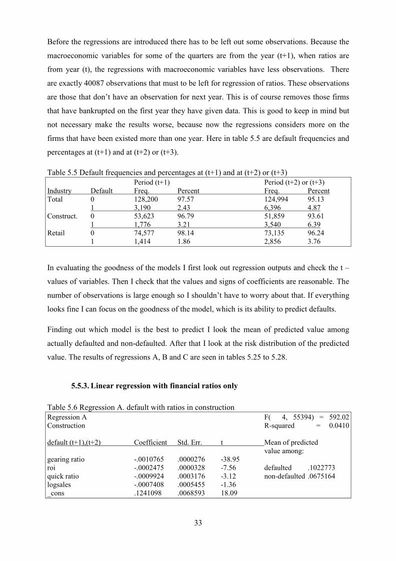
Before the regressions are introduced there has to be left out some observations. Because the

macroeconomic variables for some of the quarters are from the year (t+1), when ratios are

from year (t), the regressions with macroeconomic variables have less observations. There

are exactly 40087 observations that must to be left for regression of ratios. These observations

are those that don’t have an observation for next year. This is of course removes those firms

that have bankrupted on the first year they have given data. This is good to keep in mind but

not necessary make the results worse, because now the regressions considers more on the

firms that have been existed more than one year. Here in table 5.5 are default frequencies and

percentages at (t+1) and at (t+2) or (t+3).

Table 5.5 Default frequencies and percentages at (t+1) and at (t+2) or (t+3)

Period (t+1) Period (t+2) or (t+3)

Industry Default Freq. Percent Freq. Percent

Total 0 128,200 97.57 124,994 95.13

1 3,190 2.43 6,396 4.87

Construct. 0 53,623 96.79 51,859 93.61

1 1,776 3.21 3,540 6.39

Retail 0 74,577 98.14 73,135 96.24

1 1,414 1.86 2,856 3.76

In evaluating the goodness of the models I first look out regression outputs and check the t –

values of variables. Then I check that the values and signs of coefficients are reasonable. The

number of observations is large enough so I shouldn’t have to worry about that. If everything

looks fine I can focus on the goodness of the model, which is its ability to predict defaults.

Finding out which model is the best to predict I look the mean of predicted value among

actually defaulted and non-defaulted. After that I look at the risk distribution of the predicted

value. The results of regressions A, B and C are seen in tables 5.25 to 5.28.

5.5.3. Linear regression with financial ratios only

Table 5.6 Regression A. default with ratios in construction

Regression A F( 4, 55394) = 592.02

Construction R-squared = 0.0410

default (t+1),(t+2) Coefficient Std. Err. t Mean of predicted

value among:

gearing ratio -.0010765 .0000276 -38.95

roi -.0002475 .0000328 -7.56 defaulted .1022773

quick ratio -.0009924 .0003176 -3.12 non-defaulted .0675164

logsales -.0007408 .0005455 -1.36

_cons .1241098 .0068593 18.09

34

Table 5.7 Regression A. default with ratios in retail

Regression A F( 4, 75986) = 539.94

Retail R-squared = 0.0276


value among:

gearing ratio -.0005329 .0000153 -34.81

roi -.0002599 .0000234 -11.13 defaulted .0641821

quick ratio -.0007284 .000191 -3.81 non-defaulted .0335313

logsales -.0017328 .0003074 -5.64

_cons .0851499 .0040042 21.27

Here we can see the regression model A, where only financial ratios are represented. We can

see that the ratios in both industries have same sort of significance levels (values). The most

significant ratio is the gearing ratio, which have t-values -38.95 and 34.81 in construction and

retail respectively. Second significant is the return on investment and third the quick ratio.

The logarithm of sales is quite significant on retail but in construction the t-value is only -1.36.

In regressions B and C I have dropped the logarithm of sales and used only the first three

ratios.

In right hand side we can see the mean of predicted value among actually defaulted and non-

defaulted. We can use these numbers when we are measuring the goodness of regression B

and see if the prediction ability is improved after adding the variables of history of defaults

and sales growth over 70 % per year.

5.5.4. Regression with already occurred default and growth variable added

Table 5.8 Regression B. default with ratios, sales growth >70 % and history of defaults

Regression B F( 5, 55393) = 1399.64



value among:

default history (t),(t-1) .4324929 .0064986 66.55

gearing ratio -.0008216 .0000269 -30.58 defaulted .168899

roi -.0002765 .0000311 -8.90 non-defaulted .0567326

quick ratio -.0010109 .0003026 -3.34

sales growth >70% .0219682 .003578 6.14

_cons .0930437 .0015137 61.47

35

Table 5.9 Regression B. default with ratios, sales growth >70 % and history of defaults

Regression B F( 5, 75985) = 1231.61



value among:

default history (t),(t-1) .3551466 .0056715 62.62

gearing ratio -.0004494 .0000149 -30.10 defaulted .1097334

roi -.0002696 .0000225 -11.97 non-defaulted .0347659

quick ratio -.0005263 .0001836 -2.87

sales growth >70% .0050641 .0023517 2.15

_cons .0540943 .0009228 58.62

Here above we can see the regression B where sales growth over 70 % and history of defaults

variables are added. We can see that the significance levels of the ratios have stayed quite

stable. The default history variable which takes into account defaults from year (t) and (t-1)

seems to have very significant role in the model. After adding the default history into the

model it is quite hard to improve the prediction ability. This makes a good sense why

payment failure registers are so much used. Also sales growth >70% seem to have some role

in both industries. When a firm is

In the right hand side we can again see the mean of predicted values among actually defaulted

and non-defaulted. We can see that the regression B work much better when we are looking

the predicted mean value among defaulted, but among non-defaulted only in construction it

has lower value, when in retail it actually has higher value than regression A. In result tables

5.25 to 5.28 we can though see also the risk classifications and we can see that regression B

works much better than regression A.

5.5.5. Regression with macroeconomic variables

There are numerous methods to use macroeconomic variables in prediction models. The

macroeconomic variables can be used alone, all together, integrated together as categorical- or

dichotomous variable, it can be used as integration variable with ratios or there can be used a

method of primary component analysis. I’m going to make regressions with multiple ways

and try to find the most valuable method.

Before I do any regressions I have to clarify how I’m going to use different quarterly

macroeconomic values with ratios and defaults. So as described before the default is used at

time (t+2) and (t+3) when ratios are used at time (t). But when we are adding the

macroeconomic variables, we have to think when we have the macroeconomic data available

36

in real life compared to the financial ratio data. Here is next in table 5.10 a list of the periods

used at different quarters.

Table 5.10

Quarter Ratios at year Default history from year Macroeconomic variables at year

1 t t and t-1 t+1

2 t t and t-1 t+1

3 t t and t-1 t+1

4 t t and t-1 t

Let’s consider that we are living at year (t+1) and the third quarter has just started. At this

point we have the financial data from year (t) and we macroeconomic data from 1st quarter of

year (t+1). We want to use the newest information so this data is what we are using. The

quarterly macroeconomic data is available about 3 months after the quarter has ended

(Tilastokeskus). The financial ratio data should also be available after about 3 months from

the end of last accounting period (year). The 4th

quarter’s macroeconomic data is from the

same year (t) as the financial ratio data. This is because when the macroeconomic data from

the 4th

quarter from year (t) is available after 3 months, the newest financial ratio data from

year (t) should also be available.

The most valuable and credible regression method founded was the one that included all the

macroeconomic variables in one dummy variable. This dummy variable gets a value 1, if at

least three out of four macroeconomic dummy variables get a value of 1, and 0 otherwise.

These four macroeconomic variables and the combined macroeconomic dummy variable are

represented in table 5.11 below. Sorensen & Whitta-Jacobsen (2010) describes in their text

book (p.358), that business cycles are characterized by a co-movement of a large number of

economic activities and not just by movements in a single variable like real GDP.

When studying the regressions with financial ratios and macroeconomic variables when

financial ratios where dealt all together but separately as own variables, the results are not so

clear. The significance level of macroeconomic variables vary between

37

Table 5.11. Macroeconomic variables

Macroeconomic variable Value description Dummy gets values:

a. Gross national income % change to same quarter last year � 1, "# $ < 00 '(ℎ�*+",�

-

b. Industry volume % change to same quarter last year � 1, "# $ < 00 '(ℎ�*+",�

-

c. Consumption % change to last quarter � 1, "# $ < 00 '(ℎ�*+",�

-

d. Consumer confidence Descriptive number � 1, "# $ < 120 '(ℎ�*+",�

- on economy

Combined macro- Combined from variables above �1, "# / + 1 + 2 + 3 > 20 '(ℎ�*+",�

- economic dummy

variable

Table 5.12. Regression with economic downturn dummy variable

Regression C. F( 6, 55392) = 1206.37


Ratiodata available from (t)

Macrodata available from (t+1) 1st quarter Mean of predicted

value among:

default (t+1),(t+2) Coefficient Std. Err. t

defaulted .1720859

default history (t),(t-1) .4297769 .0064889 66.23 non-defaulted .0565151

gearing ratio -.0008193 .0000268 -30.55

roi -.0002471 .0000311 -7.96

quick ratio -.0011912 .0003022 -3.94

sales growth >70% .0231638 .0035721 6.48

economic downturn .0332713 .0022785 14.60

_cons .0845546 .0016188 52.23


Regression C. F( 6, 55392) = 1184.88



Macrodata available from (t+1) 2nd

quarter Mean of predicted

value among:


defaulted .1703778


gearing ratio -.0008183 .0000269 -30.47

roi -.0002757 .000031 -8.88

quick ratio -.0010786 .0003024 -3.57

sales growth >70% .0222684 .003575 6.23


_cons .0894924 .001554 57.59

38


Regression C. F( 6, 55392) = 1203.45



Macrodata available from (t+1) 3rd


value among:


defaulted .1718543


gearing ratio -.0008147 .0000268 -30.37

roi -.0002809 .000031 -9.06

quick ratio -.0011101 .0003021 -3.67

sales growth >70% .0224221 .0035719 6.28


_cons .0857129 .0015984 53.62


Regression C. F( 6, 55392) = 1184.88



Macrodata available from (t) 4th quarter Mean of predicted

value among:


defaulted .1703778


gearing ratio -.0008183 .0000269 -30.47

roi -.0002757 .000031 -8.88

quick ratio -.0010786 .0003024 -3.57

sales growth >70% .0222684 .003575 6.23


_cons .0894924 .001554 57.59


Regression C. F( 6, 75984) = 1043.90



Macrodata available from (t+1) 1st quarter Mean of predicted

value among:


defaulted .1108745


gearing ratio -.000448 .0000149 -30.03

roi -.0002655 .0000225 -11.79

quick ratio -.0005566 .0001835 -3.03

sales growth >70% .0058018 .0023513 2.47


_cons .0517618 .000952 54.37

39


Regression C. F( 6, 75984) = 1043.90



Macrodata available from (t+1) 2nd


value among:


defaulted .1108745


gearing ratio -.000448 .0000149 -30.03

roi -.0002655 .0000225 -11.79

quick ratio -.0005566 .0001835 -3.03

sales growth >70% .0058018 .0023513 2.47


_cons .0517618 .000952 54.37


Regression C. F( 6, 75984) = 1062.21



Macrodata available from (t+1) 3rd


value among:


defaulted .1120608


gearing ratio -.000445 .0000149 -29.84

roi -.0002676 .0000225 -11.89

quick ratio -.0005874 .0001834 -3.20

sales growth >70% .0063671 .0023504 2.71


_cons .0491978 .0009847 49.96


Regression C. F( 6, 75984) = 1043.90



Macrodata available from (t) 4th quarter Mean of predicted

value among:


defaulted .1108745


gearing ratio -.000448 .0000149 -30.03

roi -.0002655 .0000225 -11.79

quick ratio -.0005566 .0001835 -3.03

sales growth >70% .0058018 .0023513 2.47


_cons .0517618 .000952 54.37

From the regression C outputs we can see that the control variables (regression B) still has

same kind of role in the model. The macroeconomic variable called economic downturn has

also significant role in both industries and in all quarters. The results of mean of predicted

values among actually defaulted and non-defaulted are represented in tables 5.25 to 5.28.

40

5.5.6. Results of regression B with macroeconomic variables added one by one

First I introduce the macroeconomic variables individually with control group of financial

ratio variables, occurred defaults and too fast growth of sales. The mean of predicted values

among actually defaulted are compared to the corresponding values of regression B. This tells

if the added variable give new prediction value. The mean of predicted value among actually

non-defaulted is left aside at this point, because the changes in the value are so small.

Table 5.20

Gross national income percentage change to last year corresponding quarter

Mean of predicted value

Variable time serie coefficient std. error t –value among actually defaulted

Construction Reg. B

.168899

gni4 (t) Q4 -.0026241 .0002558 -10.26 .1704746

gni1 (t+1) Q1 -.0025111 .0002007 -12.51 .1712411

gni2 (t+2) Q2 -.0023131 .0002791 -8.29 .1699285

gni3 (t+3) Q3 -.0044185 .000328 -13.47 .1716129

Retail Reg. B

.1097334

gni4 (t) Q4 -.0017007 .0001848 -9.20 .110725

gni1 (t+1) Q1 -.0016578 .00014 -11.84 .1113736

gni2 (t+2) Q2 -.0016127 .0001948 -8.28 .1105357

gni3 (t+3) Q3 -.0030555 .0002286 -13.37 .1118227

In table 5.20 we can see the macroeconomic variable of gross national income. From t-values

we can see that the variable is significant and it negatively correlates with the future defaults.

From the predicted mean values among actually defaulted we can see that GNI alone gives

some new value to the regression B. No clear difference between industries.

Table 5.21

Consumer confidence on economy (dummy variable)

1 if x < 12 , 0 if x ≥ 12



Construction Reg. B

.168899

confidum4 (t) Q4 .0043965 .0023095 1.90 .1689533

confidum1 (t+1) Q1 .0120169 .0025539 4.71 .169231

confidum2 (t+2) Q2 .0049767 .0019672 2.53 .168995

confidum3 (t+3) Q3 .0010727 .0019991 0.54 .1689033

Retail Reg. B

.1097334

confidum4 (t) Q4 .0034131 .0015464 2.21 .1097905

confidum1 (t+1) Q1 .0084826 .0017478 4.85 .1100093

confidum2 (t+2) Q2 .0037336 .0013344 2.80 .1098251

confidum3 (t+3) Q3 .0013819 .0013593 1.02 .1097455

41

In table 5.21 we can see the macroeconomic variable of consumer confidence on economy,

which is represented in dummy form. The dummy form is used because the consumer

confidence is a descriptive number. From t –values we can see that it is merely significant and

the actual consumer confidence variable (not the dummy) correlates negatively with future

defaults. The t –values are quite low in this kind of large data, so using this variable alone

might not be recommended. With other variables as integration variable this might give some

information to the current macroeconomic state. From predicted values among actually

defaulted we can see that there might be some value in this variable for making the regression

model B better. No clear difference between industries.

Table 5.22

Consumption percentage change to last quarter



Construction Reg. B

.168899

consuq4 (t) Q4 -.0189688 .0016828 -11.27 .1708009

consuq1 (t+1) Q1 -.0005356 .0009406 -0.57 .1689038

consuq2 (t+2) Q2 -.0097701 .0011915 -8.20 .1699065

consuq3 (t+3) Q3 -.0078001 .0012845 -6.07 .1694519

Retail Reg. B

.1097334

consuq4 (t) Q4 -.0128375 .0011742 -10.93 .1111316

consuq1 (t+1) Q1 -.000042 .0006653 -0.06 .1097335

consuq2 (t+2) Q2 -.0062477 .0008215 -7.61 .1104106

consuq3 (t+3) Q3 -.0049692 .0008713 -5.70 .1101144

In table 5.22 we can see the macroeconomic variable of consumption. From t- values we can

see that it is significant except in (t+1) Q1. This might be because the growth of consumption

has been quite stable in the whole period. The only small decline in consumption is in 2008

financial crisis. This low volatility is also the reason why this variable is measured as

percentage change to last quarter and not to last year corresponding quarter as the other

variables are. In any case I call this variable significant and it negatively correlates with future

defaults. From predicted mean values among actually defaulted we can see that this variable

gives some new value to the regression B. No clear difference between industries.

42

Table 5.23

Industry volume percentage change to last year corresponding quarter



Construction Reg. B

.168899

conq4y (t) Q4 -.0009582 .000117 -8.19 .1699043

conq1y (t+1) Q1 -.001756 .0001799 -9.76 .1703262

conq2y (t+2) Q2 -.0008691 .0001733 -5.01 .1692761

conq3y (t+3) Q3 -.0006356 .0001495 -4.25 .16917

Retail Reg. B

.1097334

retq4y (t) Q4 -.0002381 .0001157 -2.06 .1097831

retq1y (t+1) Q1 -.0004094 .0001161 -3.52 .109879

retq2y (t+2) Q2 -.0003372 .0001015 -3.32 .1098627

retq3y (t+3) Q3 -.0003634 .0000978 -3.72 .1098952

In table 5.23 we can see the macroeconomic variable of industry volume. This variable is

different number in industries. From t –values we can see that the variable is significant and

negatively correlates with the future defaults. There is some quite remarkable difference

between industries. The construction firms correlate much stronger to the changes in industry

volumes. From the predicted mean values among actually defaulted we can see that there is

some improvement to the regression B.

Table 5.24

Interest rate (euribor)



Construction Reg. B

.168899

eurq4 (t) Q4 .0024973 .0007825 3.19 .1690518

eurq1 (t+1) Q1 -.0025312 .0008813 -2.87 .1690227

eurq2 (t+2) Q2 -.0025546 .0007567 -3.38 .1690699

eurq3 (t+3) Q3 -.0020697 .0006992 -2.96 .1690304

Retail Reg. B

.1097334

eurq4 (t) Q4 .0018677 .0005446 3.43 .1098712

eurq1 (t+1) Q1 -.0013278 .0006019 -2.21 .1097904

eurq2 (t+2) Q2 -.0013848 .0005163 -2.68 .1098177

eurq3 (t+3) Q3 -.0010852 .0004787 -2.27 .1097936

In table 5.24 we can see the macroeconomic variable of interest rate. From t –values we can

see that it is not very significant, especially when take into account that (t) Q4 has positive

coefficient when others are negative. Maybe this variable could give some information, but it

might require more study of how it affects to the economy and to the default rates. Also

43

different time lags could be considered. Although it seems to give some value to the

regression B, I leave it out from my final model. No clear difference between industries.

From the regression models, where the macroeconomic variables are used individually one by

one we have seen that they are giving some new value to the model. There is however a small

problem when we want to use these variables together. Many of them are strongly correlated

with each other causing a problem of collinearity. A solution to this problem is to use them

together in one variable. This is exactly what have been done in regression C, where four

macroeconomic variables are turned into one dummy variable. There is also a little bit more

sophisticated way to do it called primary component analysis, where many variables are

brought together in one variable using different weights. I’m leaving this out of my research.

5.5.7. Result of regression models A, B and C

Here I introduce the results of the regressions A, B and C in one packet. Regression A with

financial ratios. Regression B with financial ratios, dummy of growth of sales and default

history from years’ (t) and (t-1). Regression C includes same as Regression B, but also a

macroeconomic dummy variable that represents possible economic downturn. The results are

from the linear regression model and from the logit regression model. We compare the

different regressions and see if they get better when we are moving down from regression A

to C. We also look if the “freshness” of the macroeconomic variable has some significance.

The lowest regression C has the most fresh macroeconomic data available from (t+1) Q3.

The interpretation of the results in tables 5.25, 5.26, 5.27 and 5.28 has four dimensions. First

we take a look at the mean of predicted value among actually defaulted. The value is

calculated from the predicted values that are between 0 to 1, if ignore some extreme cases

below zero in the linear regression model. In this case there are no values over 1 because of

the mean value of defaults is so low. Anyhow this problem is solved in using the logit

regression model also. When the firm is defaulted the default (dependent) variable gets a

value of 1. So among those that are defaulted, the better the result is, the closer the predicted

value is to 1. The larger the value is the smaller is the risk for Type I errors.

Second we take a look at mean of predicted value among actually non-defaulted. The lower

value it gets the better the model has worked and smaller is the risk for Type II errors. Third

we look at the percentages of risk classifications and how the regression model has distributed

the firms by their risk from the actual risk probabilities chart. The value is better the better it

fits in between the percentages around p. The most attention gets the low and high p –values

44

since they tell something how the model has distributed the low and high risk firms in the

right categories. Finally fourth we look at the number of defaulted in risk categories and see

the frequencies how the regression model has distributed the firms in the risk categories.

Table 5.25 Results of regression models’ default prediction abilities (linear model)

Linear regression Construction

Regression Mean of

& quarter predicted value

of macro among actually: Actual risk probabilities %

variable defaulted p≤0.5 0.5<p≤2 2<p≤7 7<p≤27 27p>0.27

A .1022773 1.23 1.40 3.23 11.82 20.99

B .168899 1.12 1.27 3.56 11.19 48.44

C (t) Q4 .1703778 1.07 1.24 3.61 11.13 48.51

C (t+1) Q1 .1720859 1.04 1.41 3.59 11.21 48.32

C (t+1) Q2 .1703778 1.07 1.24 3.61 11.13 48.51

C (t+1) Q3 .1718543 1.02 1.38 3.57 11.20 48.68

Number of defaulted in risk categories

non-defaulted p≤0.5 0.5<p≤2 2<p≤7 7<p≤27 27p>0.27

A .0675164 36 82 797 2540 85

B .0567326 35 88 1029 1676 712

C (t) Q4 .0566317 41 84 1020 1677 718

C (t+1) Q1 .0565151 48 93 991 1690 718

C (t+1) Q2 .0566317 41 84 1020 1677 718

C (t+1) Q3 .0565309 47 92 978 1703 720

Table 5.26 Results of regression models’ default prediction abilities (logit model)

Logit regression Construction

Regression Mean of

& quarter predicted value


variable defaulted p≤0.5 0.5<p≤2 2<p≤7 7<p≤27 27p>0.27

A .1001041 1.89 1.36 3.47 12.42 22.84

B .1690754 1.72 1.26 3.81 12.34 47.23

C (t) Q4 .1712586 1.51 1.19 3.85 12.38 47.38

C (t+1) Q1 .173694 1.45 1.22 3.86 12.22 47.93

C (t+1) Q2 .1712586 1.51 1.19 3.85 12.38 47.38

C (t+1) Q3 .1733425 1.29 1.21 3.84 12.32 47.53


non-defaulted p≤0.5 0.5<p≤2 2<p≤7 7<p≤27 27p>0.27

A .0614287 21 51 1111 2233 124

B .0567206 17 55 1446 1305 717

C (t) Q4 .0565716 15 55 1455 1292 723

C (t+1) Q1 .0564053 15 61 1439 1294 731

C (t+1) Q2 .0565716 15 55 1455 1292 723

C (t+1) Q3 .0564293 13 62 1423 1320 722

45

In tables 5.25 and 5.26 we can see the results of linear and logit regression models’ default

prediction abilities in construction. The regression models seem to get better when we add

new significant variables.

From regression A to B the prediction ability increases seemingly when previous defaults of

year (t) and (t-1) and dummy variable of fast sales growth are added. The mean of predicted

value among actually defaulted increases significantly in both models. The mean p of non-

defaulted is also decreased seemingly and though reduces the risk of Type II errors. Also the

risk classifications look much better in regression B. Both the very small risk and very high

risk actual probabilities look seemingly closer to the p –class they should be. The frequencies

are also seemingly better distributed. Regression A is almost unable to classify the very high

risk firms’ p>0.27. One unexpected observation is the higher values in p <0.005 than in

0.005<p≤0.02 in the logit model. In linear regression model this doesn’t occur. Here is one

example where the linear model might fail. The reason why this happens is probably the

possibility the linear model to get values below zero. If we look at the frequencies we see that

the linear model has accepted much more firms in the very small risk class than the logit

model. This speak something about that the linear model treats the p -value 0.005 like it is

actually higher. This is because there are values below zero and thus more than 5 % of

observations below the p<0.005. For this reason I trust more in the logit model and base

the assumptions of the results on that and leave the linear model on less attention.

From regression model B to C we also can see some improvement. The change is not large,

but there seem to be some. The mean of predicted value among defaulted and non-defaulted is

better in all quarters and the best predicted value is in year (t+1) 1st quarter. Also the very

small risk class probabilities improved slightly from B to C. In fourth quarter of regression C

the actual precentage risk in very small risk category improves to 1.29 from 1.72 from

regression B. This is almost 0.5 % and can be seen quite large change, because the category

itself is 0.5 % wide. In the very high risk class there is also little improvement. The

percentages may not tell much, but the frequencies tell that the macroeconomic variable have

found few more very high risk firms comparing to regression B.

46

Table 5.27. Results of regression models’ default prediction abilities (linear model)

Linear regression Retail

Regression

& quarter Mean of predicted value


variable defaulted p≤0.5 0.5<p≤2 2<p≤7 7<p≤27 p>27

A .0641821 0.79 1.06 3.80 12.40 4.44

B .1097334 0.89 1.02 3.64 11.69 41.21

C (t) Q4 .1108745 0.75 1.10 3.62 11.46 41.21

C (t+1) Q1 .1108745 0.75 1.10 3.62 11.46 41.21

C (t+1) Q2 .1108745 0.75 1.10 3.62 11.46 41.21

C (t+1) Q3 .1120608 0.70 1.10 3.59 11.54 41.21


non-defaulted p≤0.5 0.5<p≤2 2<p≤7 7<p≤27 p>27

A .0335313 54 165 1767 868 2

B .0347659 65 184 1648 518 441

C (t) Q4 .0347213 63 192 1605 555 441

C (t+1) Q1 .0347213 63 192 1605 555 441

C (t+1) Q2 .0347213 63 192 1605 555 441

C (t+1) Q3 .034675 67 184 1562 602 441

Table 5.27. Results of regression models’ default prediction abilities (logit model)

Logit regression Retail

Regression

& quarter Mean of predicted value


variable defaulted p≤0.5 0.5<p≤2 2<p≤7 7<p≤27 p>27

A .0628406 0.91 1.01 3.73 13.24 12.46

B .1113446 0.84 1.06 3.54 13.07 38.24

C (t) Q4 .1130827 0.79 1.06 3.57 12.43 38.52

C (t+1) Q1 .1130827 0.79 1.06 3.57 11.43 38.52

C (t+1) Q2 .1130827 0.79 1.06 3.57 11.43 38.52

C (t+1) Q3 .1146744 0.76 1.01 3.58 12.68 38.39


non-defaulted p≤0.5 0.5<p≤2 2<p≤7 7<p≤27 p>27

A .0365971 28 152 1953 684 39

B .0347029 24 191 1793 440 408

C (t) Q4 .0346351 23 203 1754 470 406

C (t+1) Q1 .0346351 23 203 1754 470 406

C (t+1) Q2 .0346351 23 203 1754 470 406

C (t+1) Q3 .0345729 23 208 1689 531 405

47

In retail in tables 5.27 and 5.28 there are similar improvements from regression A to B as in

the case of construction. This difference is quite obvious and so I move on studying the

regression C. One reason why I chose to take regression A into this paper is to show how the

prediction ability improves when new significant variables are added.

Comparing regressions from B to C small improvement in mean of actually defaulted and

non-defaulted can be observed. The best results are in regression C (t+1) Q3, where also the

p<0.005 has the smallest value 0.0076 comparing to the regression B 0.0084. This gives some

support for the hypothesis H3. Even that the differences seems quite small they might have

some value. If we look at the table 5.3 we see default percentages and probabilities of

Standard & Poor’s credit ratings. The default percentages and frequencies are very small in

AAA and AA rated firms and even a 0.1 % change in default probability can change the

whole credit rating of a firm.

The reason why the quarterly predicted values have similar answers in retail is that the

macroeconomic variable is a dummy and react only very rare situations. It has same values in

same years of quarters Q4, (t+1) Q1 and Q2 so the results are also identical.

5.5.8. Correlation between variables

The coefficient of correlation will get values between -1 and +1. If correlation coefficient is

equal to 1, the variables are perfectly positive correlated and move though to the same

direction all the time. If correlation coefficient is equal to -1, the variables are perfectly

negatively correlated and move though to the opposite direction all the time. If correlation

coefficient is equal to 0, the variables have no systematic relationship. Other values between -

1 and +1 indicate that they have some negative or positive correlation and they have co-

movement to the same or opposite direction. If the variables are highly correlated with each

other, there might rise a problem of collinearity. In the situation of collinearity it is hard to

find out which one of the variables is causing the changes in the dependent variable. There

can be seen some quite strong correlation between the macroeconomic variables. This is why

the macroeconomic variables should be treated together in one variable, either with very

simple method like I combine them into one dummy variable or in more complex forms like

in primary component analysis.

48

6. Testing regression model to test data

Testing the regression models on out-of-sample test data found to be difficult, because the

appropriate data was not available. I have some data from firms’ financial ratios and defaults.

This data is from year 1991 to year 1998. First problem of the test data was that the equations

of ratios are different and are not comparable with the sample data. Second problem is that the

early nineties there are only few firms’ information available. Also those firms that are

available are much larger firms than those in the sample data. The reason for the second

problem is that the financial data was not gathered with the same way and quantities as are

done nowadays. Third problem concerns the macroeconomic data. The consumer confidence

information is available from 1995. This data could be easily manipulated to the dummy form,

because the confidence was probably not very high in the early nineties.

All in all, the target of this paper was to evaluate the benefits of adding macroeconomic

variables into the regression model of financial ratios and other background information like

already occurred defaults. The possibility of having a change to evaluate these benefits needs

an appropriate data. This data should of course have comparable variables, but also strong

macroeconomic variation of shock(s). These shocks could be the financial crisis started in

2008 or the depression in Finland early nineties.

If I had test data I would have used the regression models B and C. I would have used the

coefficients and constant from the regression outputs and multiplied the test data variables

with those coefficients. The model would have calculated a predicted value for each

observation. Then I would have made the same mean value analysis comparing the

regressions B and C and studying if there were any improvement. Also the risk classification

analysis could have been made with the same way as in the sample data.

The difference of testing the model is that the regression coefficients and constant is

calculated from the different data and the regression line is fitted by the sample data. Using a

given model to the test data could give whole different answers than in the sample data where

the model is been made.

49

7. Results to hypothesis



Most of the macroeconomic variables are significant. The most significant is the gross

national income. The least significant are consumer confidence on economy and interest rate.

All the variables alone gave some new value to the model, but when they are used together

they raise a problem of collinearity. Many of the macroeconomic variables are highly

correlated with each other that using them together is not recommended. The problem to this

solution is to use them together in one variable. With this way also the significance level

increases. Hypothesis H1 is thus proven right and is not rejected.


From mean of predicted value analysis and risk classifications we can see that the regression

with financial ratios, occurred defaults and fast growth of sales is improved when the

macroeconomic variables are added. In this paper the macroeconomic variables are used

together in one dummy variable. This variable reacts quite rarely, but when it does, it has

some quite reliable information of the macroeconomic state. The prediction abilities do not

improve dramatically, but there is some improvement. Even that the improvement is very

small, it can be valuable information. For example the Type I errors in lending decisions (loan

is granted to a firm that defaults) can be very costly. Avoiding even few of Type I errors can

have significant savings. Also avoiding Type II errors is important. That is improvement in

finding good firms and lending money at healthy economic situations is important for the

lender and for the firms also. Hypothesis H2 is thus proven right and is not rejected.

H3: The newer the macro data used in model, the more significant the macro data is and better

it predicts the future defaults.

The results to hypothesis H3 are quite marginal. We can see some indications that the newer

macroeconomic data is more valuable, but the significance is so weak that any serious

conclusions can’t be made. The mean of predicted value of the actually defaulted, non-

defaulted and risk classifications give some indications that the model improves with newer

macroeconomic data. There is though a change for this happening on coincidence. The same

discussion as above about Type I- and Type II errors hold here too, but hypothesis H3 does

not have enough evidence and is this point rejected. Further research with more data is

recommended.

50

8. Conclusions

The ambition of this paper was widen the view of the credit ratings from firm specific view to

more macroeconomic view where also the surrounding world is taken into consideration of

predicting the default risks. The reason why a firm defaults can be an external shock that has

nothing to do with the firm’s own actions and qualities. Example of this kind of shock is the

2008 financial crisis that hit the whole world. In this paper the impacts of it can also be seen

in quickly risen number of defaults and fallen financial ratios.

Macroeconomic variables are giving new value to the prediction model, but it seems that this

value comes exposed mostly in the situations of economic shocks. In normal and smaller

business cycles these variables seem to live their own lives and alone their default prediction

value is not so credible.

The models used in this paper were quite simple and the macroeconomic variable was

represented in very simple form. I though find it good that the model and variables are simple.

It is very easy to understand how the macroeconomic variable works in the model. The

simplicity reduces the risk of wrong conclusions. Even with the simple models there was seen

some results to the hypotheses.

I think this is a very good starting point in building a new model and improve it. There are

infinite possibilities to continue from here. For future research I recommend finding new

variables. Like export and investment was not included in my models. Also improving the

models itself is one direction. One example is to use primary component analysis for the

macroeconomic variable. There are also some much more complicated models available in

literature. The data could also be expanded. There are a dozen or so industries that could be

studied and those industries include thousands of firms. Also longer time periods could be

used. In this paper there is only one large economic shock that affected to the results. The

study of business cycles could be more represented. The data of economic shocks from

history may not be easily available or doesn’t even exist, but maybe in the future when new

shocks occurs this study could be continued.

51

References

Altman E.I. Financial Ratios, Discriminant Analysis, and the Prediction of Corporate

Bankrupty, Journal of Finance 23, 1968, 589-609.

Argenti J. Predicting Corporate Failre, Accountants Digest. No 138. Summer 1983.

Amemiya T. Qualitative response models: a survey. Journal of Economic Literature 19(4),

1981 1483-1536.

Beaver W.H. Financial Ratios as Predictors of Failure, Journal of Accounting Research Vol. 4,

1966 p. 71-111.

Bharath S.T. Shumway T. Forecasting default with the Merton distance to default model,

Review of Financial Studies, Volume: 21 Issue: 3, 2008 Pages: 1339-1369.

Cantor R. & Packer F. The Credit Rating Industry, Federal Reserve Bank of New York,

Quarterly review/Summer-Fall Vol 19, Number 2, 1994.

Carling K. Jacobson T. Linde J. and Roszbach K. Corporate credit risk modeling and the

macroeconomy, Journal of Banking & Finance 31, 2007 845-868.

Chava S. Stefanescu C. Turnbull S. Modeling the Loss Distribution, Management Science,

Volume 57, Issue 7, 2011, Pages: 1267-1287.

Dougherty C. Introduction to Econometrics, Third edition, Oxford University Press 2007.

Duffie D. Saita L. Wang K. Multi-period corporate default prediction with stochastic

covariates, Journal of Financial Economics, Volume 83, Issue 3, 2007, Pages: 635-665.

Hillegeist S.A. Keating E.K. Cram D.P. Lundstedt K.G. (2004) Assessing the probability of

bankruptcy, Review of Accounting Studies, Volume 9, Issue 1, 2004, Pages: 5-34.

Horrigan J. O. A Short History of Financial Ratio Analysis, The Accounting Review, April.

1968, 284-294.

Keasey K. Watson R. Non-Financial Symptoms and the Prediction of Small Company Failure:

a Test of Argenti’s Hypotheses, Journal of Business Finance & Accounting, 14(3) Autumn

1987.

52

Koopman S.J. Lucas A. Monteiro A. The multi-state latent factor intensity model for credit

rating transitions, Journal of Econometrics 142, 2008, 399-424.

Laitinen E. K. Luottotieto ja Tiede. Majakka 2005. Suomen Asiakastieto Oy.

Long J. Scott Regression models for categorical and limited dependent variables: Advanced

quantitative techniques in social sciences v. 7, 1997, Sage Publications.

Merton R. On the Pricing of Corporate Debt: The Risk Structure of Interest Rates. Journal of

Finance 29, 1974, 449-470.

Prihti, A. Konkurssin ennustaminen taseinformaation avulla. The prediction of bankruptcy

with published financial data. Helsingin Kauppakorkeakoulu. Acta Academiae Oeconomicae

Helsingiensis, A:13. Helsinki 1975.

Foulke, Roy A. Financial Ratios Become of Age. Journal of Accountancy. September 1937.

203-213.

Sorensen & Whitta-Jacobsen Introducing Advanced Macroeconomics, Growth and Business

Cycles, Second Edition 2010. McGraw-Hill Education.

Internet:

Standard & Poor’s Annual Global Corporate Default Study And Rating Transitions 2011:

http://www.standardandpoors.com/ratings/articles/en/us/?articleType=HTML&assetID=1245

330814766

Tilastokeskus 2013:

http://www.tilastokeskus.fi/til/kan.html

Other:

Suomen Asiakastieto Oy sources 2013.

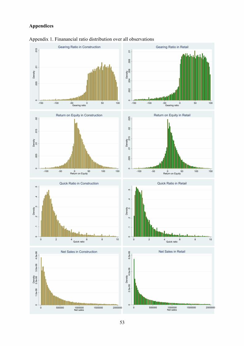
53

Appendices

Appendix 1. Finanancial ratio distribution over all observations

0.005

.01

.015

Density

-150 -100 -50 0 50 100Gearing ratio

Gearing Ratio in Construction

0.002

.004

.006

.008

.01

Density

-150 -100 -50 0 50 100Gearing ratio

Gearing Ratio in Retail

0.005

.01

.015

.02

Density

-100 -50 0 50 100 150Return on Equity

Return on Equity in Construction

0.005

.01

.015

.02

.025

Density

-100 -50 0 50 100 150Return on Equity

Return on Equity in Retail

0.1

.2.3

.4.5

Density

0 2 4 6 8 10Quick ratio

Quick Ratio in Construction

0.1

.2.3

.4.5

Density

0 2 4 6 8 10Quick ratio

Quick Ratio in Retail

01.0e-06

2.0e-06

3.0e-06

4.0e-06

Density

0 500000 1000000 1500000 2000000Net sales

Net Sales in Construction

02.0e-06

4.0e-06

6.0e-06

Density

0 500000 1000000 1500000 2000000Net sales

Net Sales in Retail

54

Appendix 2. Main yearly statistics from construction and retail

Construction mean of ratios at (t) and default percentages at (t+1)

year roi gearing quick sales % defaulted % bankrupted

1999 28.828542 39.604201 2.1376042 1362169.843 2.222222 .3472222

2000 26.705769 39.279304 2.0733822 1254052.546 2.258852 .2136752

2001 25.065766 41.73308 2.3380631 1273275.956 2.533784 .1407658

2002 21.733832 41.996269 2.4902538 1224508.565 2.690355 .1522843

2003 22.215339 41.53177 2.4047785 1106389.413 2.334715 .1090988

2004 20.468346 39.462947 2.2242874 1053844.326 2.990767 .080289

2005 21.137463 39.476536 2.2979776 1130029.069 3.004123 .1767131

2006 21.010924 39.861191 2.2956066 1175322.96 3.56224 .178112

2007 21.209915 39.080891 2.5771729 1165528.496 4.157515 .3294635

2008 18.22688 37.850696 2.6894969 1135338.135 7.06449 .990099

2009 11.729873 36.12863 2.6914595 1024789.849 7.235206 .9199404

2010 12.893372 34.734462 2.5554311 970607.2869 7.70138 .978889

2011 15.706737 35.754681 2.6459781 1054800.858 7.772936 .9186197

Construction 25 percentiles of ratios at (t) and default percentages at (t+1)

year roi25 gearing25 quick25 sales25 % defaulted % bankrupted

1999 7.6 20.45 .7 99231 2.222222 .3472222

2000 7.1 20.6 .7 104108 2.258852 .2136752

2001 5.95 22.2 .7 103082.5 2.533784 .1407658

2002 3.6 22 .7 98273.5 2.690355 .1522843

2003 3.3 21.4 .8 90962 2.334715 .1090988

2004 2.2 20 .7 87000 2.990767 .080289

2005 2.7 19.9 .7 93000 3.004123 .1767131

2006 3 20 .8 98000 3.56224 .178112

2007 2.6 18.4 .7 93588 4.157515 .3294635

2008 0 16.7 .7 86000 7.06449 .990099

2009 -3.4 14.6 .7 75000 7.235206 .9199404

2010 -2.4 14.3 .7 75000 7.70138 .978889

55

2011 0 14.9 .7 79000 7.772936 .9186197

Construction median of ratios at (t) and default percentages at (t+1)


1999 24.6 42.8 1.3 280285 2.222222 .3472222

2000 22.9 44.1 1.3 294665.5 2.258852 .2136752

2001 21.8 47.1 1.3 288792.5 2.533784 .1407658

2002 18.9 47.6 1.3 267820.5 2.690355 .1522843

2003 18.2 46.7 1.4 251197 2.334715 .1090988

2004 16.9 44.4 1.3 249000 2.990767 .080289

2005 17.3 44.3 1.3 261501 3.004123 .1767131

2006 17.5 45 1.3 283876 3.56224 .178112

2007 17.5 44.3 1.4 265447 4.157515 .3294635

2008 14.3 44.15 1.4 243026.5 7.06449 .990099

2009 8.8 45.2 1.4 203000 7.235206 .9199404

2010 10.1 43.1 1.3 211000 7.70138 .978889

2011 12 43.8 1.4 227000 7.772936 .9186197

Construction 75 percentiles of ratios at (t) and default percentages at (t+1)


1999 48.2 63.2 2.1 813861.5 2.222222 .3472222

2000 45.15 65.45 2.3 849601.5 2.258852 .2136752

2001 42.65 69 2.5 818948.5 2.533784 .1407658

2002 38.6 70.95 2.5 774122 2.690355 .1522843

2003 39.1 69.5 2.6 676351 2.334715 .1090988

2004 38.5 66.7 2.4 673000 2.990767 .080289

2005 37.5 67.9 2.4 727025 3.004123 .1767131

2006 36.9 68.6 2.4 803759 3.56224 .178112

2007 37.8 69.4 2.6 748136 4.157515 .3294635

2008 35.8 71.4 2.8 729463 7.06449 .990099

2009 27.8 71.8 2.9 602340 7.235206 .9199404

2010 28.2 70.5 2.6 614000 7.70138 .978889

2011 32.3 70.3 2.7 688000 7.772936 .9186197

56

Retail mean of ratios at (t) and default percentages at (t+1)

year roi gearing quick sales % defaulted % bankrupted

1999 21.203833 37.173044 2.102398 2447069.31 1.382811 .1050236

2000 21.244539 36.241772 2.2388243 2443713.935 1.440969 .0818733

2001 20.472496 37.45669 2.3076525 2570744.013 1.213396 .0647144

2002 18.107816 36.759797 2.3850008 2431805.647 1.757361 .138739

2003 17.618129 36.38635 2.3521181 2227026.04 1.740123 .0855798

2004 18.307806 34.489897 2.1474778 2139214.685 1.736159 .1093643

2005 16.841294 34.070958 2.2209989 2306179.035 1.779801 .1241722

2006 17.562592 34.776603 2.3261933 2443720.82 2.04978 .0732064

2007 16.873907 33.009999 2.4914313 2166617.484 2.719494 .2461611

2008 13.324572 31.163442 2.6137628 2055804.568 4.366438 .6956336

2009 7.9052026 29.417887 2.5922928 1895320.403 4.374933 .4299688

2010 10.691651 28.308805 2.4448726 1972045.827 4.681997 .5386369

2011 11.466733 28.252937 2.4979857 2069351.271 4.448174 .3881662

Retail 25 percentiles of ratios at (t) and default percentages at (t+1)


1999 4 16.3 .6 129505 1.382811 .1050236

2000 4.5 16 .6 139764 1.440969 .0818733

2001 4 16.7 .6 135559 1.213396 .0647144

2002 2.5 16.6 .6 128570 1.757361 .138739

2003 1.9 15.9 .5 117106 1.740123 .0855798

2004 2 15.2 .5 105000 1.736159 .1093643

2005 .9 14.25 .5 113000 1.779801 .1241722

2006 2 14.8 .6 123000 2.04978 .0732064

2007 1 13.5 .5 95000 2.719494 .2461611

2008 0 11.8 .5 79214.5 4.366438 .6956336

2009 -3.8 10.5 .5 72000 4.374933 .4299688

2010 -1.6 9.9 .5 70000 4.681997 .5386369

2011 -1.7 9.7 .5 70000 4.448174 .3881662

57

Retail median of ratios at (t) and default percentages at (t+1)


1999 17.8 39.5 1 472440 1.382811 .1050236

2000 18.1 40.8 1.1 484213 1.440969 .0818733

2001 17.2 41.9 1.1 500864 1.213396 .0647144

2002 15.2 42.3 1.1 456722 1.757361 .138739

2003 14.3 42.9 1.1 414000 1.740123 .0855798

2004 14.4 41.1 1.1 379000 1.736159 .1093643

2005 13.1 41 1.1 409000 1.779801 .1241722

2006 14.5 41.7 1.1 453000 2.04978 .0732064

2007 13.4 41.4 1.1 375000 2.719494 .2461611

2008 10.2 41.55 1.1 323000 4.366438 .6956336

2009 6.3 41.1 1.1 297000 4.374933 .4299688

2010 7.9 40 1.1 295648.5 4.681997 .5386369

2011 8.4 39.8 1.1 298500 4.448174 .3881662

Retail 75 percentiles of ratios at (t) and default percentages at (t+1)


1999 38.1 64.2 2 1705426 1.382811 .1050236

2000 36.7 65.8 2 1709462 1.440969 .0818733

2001 34.9 67.6 2.1 1769776 1.213396 .0647144

2002 33.1 68.7 2.2 1677762 1.757361 .138739

2003 32.8 69 2.2 1536269 1.740123 .0855798

2004 33.4 66.7 2.1 1404639 1.736159 .1093643

2005 31.3 67.55 2.1 1513869 1.779801 .1241722

2006 31.6 68.8 2.2 1630000 2.04978 .0732064

2007 31.1 70.2 2.3 1384241 2.719494 .2461611

2008 27.6 71.8 2.4 1233120.5 4.366438 .6956336

2009 21.2 72.2 2.4 1089000 4.374933 .4299688

2010 24 70 2.3 1131300 4.681997 .5386369

2011 24.5 69.7 2.3 1195500 4.448174 .3881662

corporate default prediction with financial ratios and macroeconomic variables

Documents