corporate governance, product market competition, and ...xg2285/pmc2.pdf · corporate governance,...
TRANSCRIPT

THE JOURNAL OF FINANCE • VOL. LXVI, NO. 2 • APRIL 2011
Corporate Governance, Product MarketCompetition, and Equity Prices
XAVIER GIROUD and HOLGER M. MUELLER∗
ABSTRACT
This paper examines whether firms in noncompetitive industries benefit more fromgood governance than do firms in competitive industries. We find that weak gov-ernance firms have lower equity returns, worse operating performance, and lowerfirm value, but only in noncompetitive industries. When exploring the causes of theinefficiency, we find that weak governance firms have lower labor productivity andhigher input costs, and make more value-destroying acquisitions, but, again, only innoncompetitive industries. We also find that weak governance firms in noncompeti-tive industries are more likely to be targeted by activist hedge funds, suggesting thatinvestors take actions to mitigate the inefficiency.
ECONOMISTS OFTEN ARGUE THAT managers of firms in competitive industries havestrong incentives to reduce slack and maximize profits, or else the firm willgo out of business.1 Accordingly, the need to provide managers with incentivesthrough good governance—and thus the benefits of good governance—should besmaller for firms in competitive industries. In contrast, firms in noncompetitiveindustries, where lack of competitive pressure fails to enforce discipline onmanagers, should benefit relatively more from good governance.
That firms with good governance have better performance on average is wellestablished. In a seminal article, Gompers, Ishii, and Metrick (2003, GIM) findthat a hedge portfolio that is long in good governance firms (“Democracy firms”)and short in weak governance firms (“Dictatorship firms”) earns a monthlyalpha of 0.71%. Governance is measured using the G-index, which consists of24 antitakeover and shareholder rights provisions. In addition to showing thatgood governance is associated with higher equity returns, GIM also show thatit is associated with both higher firm value and better operating performance.2
∗Giroud is at the NYU Stern School of Business. Mueller is at the NYU Stern School of Business,NBER, CEPR, and ECGI. We thank Cam Harvey (the Editor), an associate editor, two anonymousreferees, and seminar participants at NYU, Yale, Michigan, Illinois, the WFA Meetings in SanDiego (2009), and the Harvard Law School/Sloan Foundation Corporate Governance ResearchConference (2009) for helpful comments. We are especially grateful to Wei Jiang and MartijnCremers for providing us with data.
1 Fritz Machlup’s (1967) presidential address to the American Economic Association containsan extensive discussion of this argument. More recent (theory) literature is discussed in Section I.
2 The evidence is not causal, though GIM examine alternative hypotheses and find no evidencethat their results are driven by either reverse causality or an omitted variable bias. That said, otherpapers show that governance has a causal effect on firm performance using exogenous variation in
563

564 The Journal of Finance R©
The evidence presented in this paper supports the hypothesis that firmsin noncompetitive industries benefit more from good governance than dofirms in competitive industries. When competition is measured using theHerfindahl–Hirschman index (HHI), we find that the alpha earned by theDemocracy–Dictatorship hedge portfolio is small and insignificant in the low-est HHI tercile, is monotonically increasing across HHI terciles, and is largeand significant in the highest HHI tercile. This pattern is robust across manyspecifications—it holds for different governance measures, different competi-tion measures, different asset pricing models, and different sample periods.The latter robustness check is particularly interesting, as prior research showsthat GIM’s results all but disappear if the sample period is extended beyond1999 (e.g., Core, Guay, and Rusticus (2006)). If we extend the sample periodto 2006, we also find that the average alpha across all firms is small and in-significant. However, the alpha in the highest HHI tercile remains large andsignificant.
There are two potential explanations for the positive alpha earned by theDemocracy–Dictatorship hedge portfolio. One is that it may be driven by anomitted variable bias. Such a bias could arise if the G-index is correlated withrisk characteristics that are priced during the sample period but that are notcaptured by the underlying asset pricing model. We address this issue in twoways. First, we extend the four-factor model to include additional risk factorsthat have been proposed in the literature. Second, we follow GIM and esti-mate Fama–MacBeth return regressions that include a broad array of controlvariables. Our results are robust in either case.
The other explanation is that weak governance gives rise to agency costswhose magnitude is underestimated by investors. To test this hypothesis, Coreet al. (2006) examine whether analysts correctly predict that weak governancefirms have lower earnings than do good governance firms. The authors find thatthe forecast error (difference between actual and forecasted earnings) is smalland insignificant, which leads them to conclude that analysts are not surprised.Consistent with this result, we also find that the average forecast error is smalland insignificant. However, the forecast error in the highest HHI tercile islarge and significant. Thus, analysts underestimate the effect of governance onearnings in precisely those industries in which governance matters for earn-ings, namely, noncompetitive industries. Whether the forecast error is largeenough to fully explain the abnormal return to the Democracy–Dictatorshiphedge portfolio remains an open question. At a minimum, it provides evidencein support of the hypothesis that investors are surprised and, consequently,that the abnormal return may not be driven by an omitted variable bias.
We obtain similar results when considering either firm value (Tobin’s Q) oroperating performance (return on assets (ROA), net profit margin, sales growth,return on equity (ROE)). The relationship between governance and either firmvalue or operating performance is always small and insignificant in the low-est HHI tercile, is monotonic across HHI terciles, and is large and significant
governance in the form of state antitakeover laws (e.g., Bertrand and Mullainathan (2003), Giroudand Mueller (2010)).

Corporate Governance, Product Market Competition 565
in the highest HHI tercile. Our operating performance results are consistentwith results in Giroud and Mueller (2010). In that paper, we find that firmsin noncompetitive industries experience a significant drop in operating perfor-mance after the passage of state antitakeover laws, while firms in competitiveindustries experience no significant effect. Unlike the present paper, however,the other paper does not consider firm-level governance instruments, nor doesit consider long-horizon equity returns or firm value.
Overall, our results suggest that, absent competitive pressure from the prod-uct market, weak governance gives rise to agency costs. To gain a better un-derstanding of the nature of these agency costs, we explore in more detail therelationship between (i) governance and investment activity and (ii) governanceand productive efficiency. With respect to the former relationship, we find thatweak governance firms have higher capital expenditures and make more ac-quisitions than do good governance firms. This relationship is again small andinsignificant in the lowest HHI tercile, is monotonic across HHI terciles, and islarge and significant in the highest HHI tercile.
That weak governance firms make more acquisitions does not necessarily im-ply that these firms destroy value. However, in a recent article, Masulis, Wang,and Xie (2007) show that high G-index acquirer firms experience significantlylower cumulative abnormal returns (CARs) than do low G-index acquirer firms.Consistent with this result, we also find that high G-index acquirer firms expe-rience significantly lower CARs on average. Importantly, however, we find thatthis relationship is large and significant only in the highest HHI tercile, while itis otherwise small and insignificant. Thus, weak governance firms make morevalue-destroying acquisitions, but only in noncompetitive industries. This re-sult is noteworthy for two reasons. First, it is a possible explanation for thepattern across HHI terciles that we consistently find in our firm value and op-erating performance regressions. Second, because CARs measure unexpectedchanges in stock prices, the result suggests that the market does not fully an-ticipate the negative valuation effects of weak governance in noncompetitiveindustries. Consequently, it is also a possible explanation for the pattern acrossHHI terciles that we consistently find in our regressions of equity returns.
As for the relationship between governance and productive efficiency, we findthat weak governance firms have lower labor productivity and higher inputcosts than do good governance firms. Importantly, this relationship is againsmall and insignificant in the lowest HHI tercile, is monotonic across HHIterciles, and is large and significant in the highest HHI tercile. We also findqualitatively similar results when considering wages, though the wage resultslack statistical significance.
Overall, our results suggest that weak governance firms have lower equityreturns, worse operating performance, and lower firm value, but only in non-competitive industries. In the final part of our analysis, we examine if investorstake actions to mitigate the inefficiency. In particular, we examine if weak gov-ernance firms, especially those in noncompetitive industries, are more likelyto be targeted by activist hedge funds. Using data on hedge fund activism byBrav et al. (2008), we find that weak governance firms in noncompetitive in-dustries are more likely to be targeted by activist hedge funds than any other

566 The Journal of Finance R©
type of firm, including weak governance firms in competitive industries andgood governance firms in noncompetitive industries.3 We also find that weakgovernance firms in noncompetitive industries experience a significant drop inthe G-index after being targeted by an activist hedge fund, though this resultis based on a relatively small sample.
Several recent papers examine the interaction between governance and com-petition. Cremers, Nair, and Peyer (2008) find that firms in competitive in-dustries have relatively more takeover defenses, but only if the industry ischaracterized by long-term customer–supplier relationships (e.g., service anddurable goods industries). Kadyrzhanova and Rhodes-Kropf (2010) find thatfour particular G-index provisions that impose a delay on potential acquirers—classified board, blank check, special meeting, and written consent—interactwith competition differently than do the remaining 20 G-index provisions. Theirexplanation is that delay provisions empower target management with bar-gaining power, which results in higher takeover premia, thus (partly) offsettingthe negative entrenchment effects of these provisions. Finally, Guadalupe andPerez-Gonzalez (2010) find that firms in countries with tighter product and in-put market regulations exhibit greater private benefits of control, as measuredby the voting premium between shares with differential voting rights.
The rest of this paper is organized as follows. Section I reviews the the-ory literature. Section II describes the data and provides summary statistics.Section III examines the relationship between governance and long-horizonequity returns, and Section IV examines the relationship between governanceand either firm value or operating performance. Section V explores the under-lying agency costs associated with weak governance. Section VI examines thelikelihood of being targeted by activist hedge funds. Section VII concludes.
I. Theory Literature
Several theory models analyze the implications of product market compe-tition for managerial slack and the resulting need to provide managers withmonetary incentives. If better governance is a substitute for monetary incen-tives, then the predictions of these models can be tied directly to the results inthis paper.
In Hart’s (1983) model, product market competition unambiguously reducesmanagerial slack. By assumption, managers care only about reaching a givenprofit target. Thus, if input costs fall, managers work less hard. In a competitiveproduct market, however, cost reductions that are common across all firms areaccompanied by falling prices. Thus, managers cannot afford to slack off butmust instead work hard to fulfill their given profit target. Importantly, in Hart’smodel, managerial income is independent of competition.4
3 We are grateful to Wei Jiang for providing us with the data.4 In Hart’s model, managers care only about reaching a given subsistence level of income, I.
Income above this level has no value, while income below it is catastrophic. Thus, as long asmanagers fulfill their given profit target, income will always be I. As Scharfstein (1988) shows, if

Corporate Governance, Product Market Competition 567
One possible channel through which competition may affect managerial in-come is through relative performance evaluation. If productivity shocks are cor-related across firms, then an increase in the number of competitors may provideadditional information that can be used to mitigate moral hazard (Holmstrom(1982), Nalebuff and Stiglitz (1983)). However, while firm owners are alwaysbetter off, the effect on managerial incentives is ambiguous. Depending on theunderlying probability distribution, the cost of implementing low effort may bereduced to a greater or lesser degree than the cost of implementing high ef-fort. As a result, it may be optimal to give managers either weaker or strongermonetary incentives.
In Schmidt’s (1997) model, an increase in competition increases the proba-bility that a firm with high costs becomes unprofitable and must be liquidated.This induces managers to work hard in order to keep their jobs and avoid thedisutility of liquidation (“threat-of-liquidation effect”). Moreover, the increasedpunishment in the event a manager is not successful makes it cheaper to im-plement a higher level of effort, making it optimal to give managers strongermonetary incentives. On the other hand, a reduction in profits caused by anincrease in competition may lower the value of a cost reduction and thus alsothe benefit of inducing higher effort (“value-of-a-cost-reduction effect”).5 As aresult, it may be optimal to give managers weaker monetary incentives. Thus,the overall effect of competition on monetary incentives is (again) ambiguous.
Raith (2003) analyzes the role of competition for monetary incentives in amodel with free entry. When the number of firms is fixed, he finds two oppositeeffects, which happen to exactly cancel each other. For instance, an increase incompetition due to greater product substitutability makes it easier for firms tosteal demand from rivals, making it optimal to give managers stronger mon-etary incentives (“business-stealing effect”). On the other hand, an increasein product substitutability results in lower prices and reduces the value of acost reduction, making it optimal to give managers weaker monetary incen-tives. With free entry, the effect of competition is no longer ambiguous. Forinstance, an increase in product substitutability results in lower profits forany given number of firms, inducing some firms to exit. Each surviving firmproduces larger output, making it unambiguously optimal to give managersstronger monetary incentives. However, the result is the opposite if competi-tion increases due to a reduction in entry costs. In this case, new firms enterthe market, each firm produces less output, and it becomes optimal to givemanagers weaker monetary incentives. Thus, for any given source of varia-tion in competition, an increase in competition has an unambiguous effect onmonetary incentives. However, as Raith (2003, p. 1430) acknowledges, “the re-lationship between competition and managerial incentives depends on whatcauses variations in the degree of competition, which poses a challenge to em-pirical tests.”
managerial utility is increasing in income, then Hart’s main result that product market competitionreduces managerial slack can be reversed.
5 A similar effect is also present in Hermalin’s (1992) model, where it is called “change-in-the-relative-value-of-actions effect.”

568 The Journal of Finance R©
As this brief overview of the theory literature shows, there are plausiblearguments for why monetary incentives may be either weaker or stronger incompetitive industries. More generally, substituting better governance for mon-etary incentives, the need to provide managers with incentives through goodgovernance—and thus the benefits of good governance—may be either weaker(substitutes) or stronger (complements) in competitive industries. Sorting outthese competing hypotheses is an empirical question, and the objective of thispaper is to examine which, if any, is consistent with the data.
II. Data
A. Sample Selection and Definition of Variables
Our sample consists of all firms in the Investor Responsibility ResearchCenter (IRRC) database that have a match in both CRSP and Compustat.Following GIM, we exclude all firms with dual-class shares. To match firms toindustries, we, moreover, require a nonmissing SIC code in Compustat. Overthe sample period from 1990 to 2006, this leaves us with 3,241 companies.
Our main measure of corporate governance is the G-index introduced byGIM. The index is constructed by adding one index point for each of the 24(anti-)governance provisions listed in GIM. Higher index values imply weakergovernance. GIM refer to companies with a G-index of 5 or less as Democraciesand to companies with a G-index of 14 or higher as Dictatorships. The G-index is obtained from the IRRC database and is available for the years 1990,1993, 1995, 1998, 2000, 2002, 2004, and 2006 during the sample period. Forintermediate years, we always use the G-index from the latest available year.In robustness checks, we also use the E-index of Bebchuk, Cohen, and Ferrell(2009) and the Alternative Takeover Index (ATI) of Cremers and Nair (2005,CN). The E-index consists of 6 of the 24 provisions listed in GIM. The ATIindex consists of three of these provisions.6 We construct the E-index and theATI index using IRRC data. The correlation between all three indices is high.Using all IRRC years, the correlation between the G-index and the E-index is0.71, the correlation between the G-index and the ATI index is 0.68, and thecorrelation between the E-index and the ATI index is 0.76.
Our main measure of product market competition is the HHI. The HHI iscomputed as the sum of squared market shares,
HHIjt :=Nj∑
i=1
s2ijt,
where sijt is the market share of firm i in industry j in year t. Market sharesare computed from Compustat using firms’ sales (item #12). When computing
6 For the E-index, we use a cutoff of E = 0 for Democracy firms and E ≥ 4 for Dictatorshipfirms. Using a cutoff of E ≥ 4 ensures that the Dictatorship portfolio contains sufficiently manycompanies relative to the Democracy portfolio (see Table II in Bebchuk et al. (2009)). For the ATIindex, we use a cutoff of ATI = 0 for Democracy firms and ATI ≥2 for Dictatorship firms.

Corporate Governance, Product Market Competition 569
the HHI, we use all available Compustat firms, including those with dual-class shares. We exclude firms for which sales are either missing or negative.The HHI is a commonly used measure in the empirical industrial organizationliterature and is well grounded in theory (see Tirole (1988), pp. 221–223). Inrobustness checks, we also use the “four-firm concentration ratio,” which is thesum of market shares of the four largest firms in an industry. This measure isalso common in the empirical industrial organization literature and is routinelyused by government agencies.
We classify industries using the 48 industry classification scheme of Famaand French (1997, FF). We assign firms to industries by matching the SICcodes of Compustat to the 48 FF industries using the conversion table in theappendix of FF. In robustness checks, we also use four-digit SIC industries.
As our competition measures are computed from Compustat, they only in-clude publicly traded companies. In robustness checks, we also use competi-tion measures provided by the Census Bureau, which include all public andprivate companies in the United States. Although these measures are morecomprehensive, they have several drawbacks. First, they are only available formanufacturing industries, which means the sample is much smaller. Second,the measures are only computed every 5 years. Because our sample period isfrom 1990 to 2006, we use data from the 1987, 1992, 1997, and 2002 Censuses.For intermediate years, we always use data from the latest available Census.Third, the measures are not available for the 48 FF industries. In the 1987 and1992 Censuses, they are only available for four-digit SIC industries. In 1997,the Census Bureau switched from SIC to NAICS codes and has since providedcompetition measures for various NAICS partitions. In our empirical analysis,we use four-digit SIC codes before 1997 and four-digit NAICS codes after 1997.We obtain similar results if we use five- or six-digit NAICS codes after 1997.
B. Empirical Relation between the G-Index and the HHI
Using all firm-year observations from 1990 to 2006, we find that the corre-lation between the G-index and the HHI is virtually zero. (The correlation is0.00 with a p-value of 0.50.) This fact has already been noted by GIM (p. 119),who conclude that “[t]here is no obvious industry concentration among thesetop firms [in the Democracy and Dictatorship portfolios].” Because the HHI isan industry measure, we can also compute the correlation at the industry level.Here, we find a weakly negative correlation of −0.06 (p-value of 0.08) betweenthe HHI and the mean G-index of an industry, which is similar to what Cremerset al. (2008) find.
The Internet Appendix contains further statistics.7 First, we divide boththe Democracy and the Dictatorship portfolio into quintiles by ranking firmsaccording to their HHIs and then sorting them into HHI quintiles. We findthat in any given HHI quintile, the empirical distribution of the HHI in the
7 The Internet Appendix is available on the Journal of Finance website at http://www.afajof.org/supplements.asp.

570 The Journal of Finance R©
Democracy and Dictatorship portfolios is virtually identical. For instance, firmsin the lowest HHI quintile of the Democracy portfolio have a mean (median)HHI of 0.02 (0.02), as do firms in the lowest HHI quintile of the Dictatorshipportfolio. Second, when we divide the full sample (not just Democracy andDictatorship firms) into HHI quintiles, we find that the mean G-index is similar,and the median G-index is identical, in all five quintiles. Importantly, there isno systematic trend. Effectively, this means that it does not matter if we sortfirms first by their G-index and then by their HHI, or the other way around.We obtain similar results if we use the E-index or the ATI index, if we use theHHI provided by the Census Bureau, if we use the original sample period inGIM (1990 to 1999) or the post-GIM period (2000 to 2006), and if we use HHIterciles or quartiles instead of quintiles.
III. Corporate Governance and Equity Returns
A. Hedge Portfolios
Our first set of results concerns trading strategies that are jointly based oncorporate governance and competition. Following GIM, we compute abnormalreturns using Carhart’s (1997) four-factor model. The abnormal return is theintercept α of the regression
Rt = α + β1 × RMRFt + β2 × SMBt + β3 × HMLt + β4 × UMDt + εt, (1)
where Rt is the excess portfolio return in month t, RMRFt is the return on themarket portfolio minus the risk-free rate, SMBt is the size factor (small minusbig), HMLt is the book-to-market factor (high minus low), and UMDt is the mo-mentum factor (up minus down). We construct portfolio returns using monthlyreturn data from CRSP. The RMRF, SMB, and HML factors are obtained fromKenneth French’s website. The UMD factor is constructed using the proceduredescribed in Carhart (1997).
GIM construct a hedge portfolio that is long in Democracy firms (G-index of5 or less) and short in Dictatorship firms (G-index of 14 or higher). To analyzethe interaction between corporate governance and competition, we divide boththe Democracy and the Dictatorship portfolio into three equal-sized portfoliosby ranking firms according to their HHIs and then sorting them into HHIterciles. This yields 2 × 3 = 6 portfolios: one Democracy and one Dictator-ship portfolio for each HHI tercile.8 For each HHI tercile, we then constructa Democracy–Dictatorship hedge portfolio analogous to GIM. By construction,this implies that all three hedge portfolios contain the same number of stocks.
Our choice of HHI terciles balances two concerns. If too many HHI groupsare formed, the number of stocks in each hedge portfolio may be too smallto allow for reliable statistical inference. On the other hand, if too few HHI
8 Our results are unchanged if we sort firms first by their HHIs and then according to whetherthey are Democracy or Dictatorship firms. This is not surprising, given that the correlation betweenthe HHI and the G-index at the firm level is virtually zero.

Corporate Governance, Product Market Competition 571
groups are formed, the spread in the HHI across hedge portfolios may not bestatistically significant. Using HHI terciles, each hedge portfolio contains onaverage 75 stocks per month, and the average monthly HHI spread (differencebetween the mean HHI in the lowest and highest HHI tercile) is 0.101, whichis statistically significant at all reasonable levels (p = 0.000). An alternativeway of sorting stocks into HHI terciles would be to use industry- rather thanfirm-level HHI cutoffs. This would produce an HHI spread of 0.127 (p = 0.000),which is slightly larger. Also, all three hedge portfolios would contain the samenumber of industries by construction. However, because competitive industrieshave more firms, the number of stocks in each hedge portfolio would no longerbe identical. Although the average number of stocks in the low HHI portfoliowould be 114, the average number of stocks in the high HHI portfolio wouldbe only 43. Because smaller portfolios are more volatile, this implies that theabnormal return in the high HHI portfolio would be estimated with more noise,making comparisons across HHI terciles difficult. For this reason, we use firm-level HHI cutoffs throughout.9
To facilitate comparison with GIM’s original results, we use the same sam-ple period, namely, September 1990 to December 1999 (112 monthly returns).In robustness checks, we extend the sample period to December 2006. We re-balance all portfolios in September 1990, July 1993, July 1995, and February1998, which are the months after which new IRRC data became available.When extending the sample period, we additionally rebalance in November1999, January 2002, January 2004, and January 2006. To incorporate newvalues of the HHI, we, moreover, rebalance all portfolios each July using theHHI computed from sales in the previous year. We obtain similar results if weuse the HHI computed from sales 2 years ago, or if we use a moving averageof the HHIs over the previous 3 years. We always report the results both forvalue weighted (VW) and equally weighted (EW) portfolios. To compute the VWreturn on a portfolio in month t, we weigh each individual stock return withthe stock’s market capitalization at the end of month t − 1.
B. Main Results
We first replicate GIM’s original results. For VW portfolios, GIM find thatthe Democracy–Dictatorship hedge portfolio earns a monthly abnormal returnof 0.71% (t = 2.73). We obtain a very similar result (0.69%, t = 2.71).10 Whenwe exclude companies with missing SIC codes, our result changes only slightly
9 The statistics discussed in this paragraph can be found in the Internet Appendix. As we showthere, our results are qualitatively similar when using industry-level HHI cutoffs. More precisely,while the alphas are very similar, their statistical significance in the highest HHI tercile is slightlyweaker, consistent with the smaller size of the high HHI hedge portfolio. Another way to generatea larger HHI spread would be to use HHI quartiles instead of terciles. The results are againqualitatively similar (see the Internet Appendix).
10 See the Internet Appendix for details. Although our alpha and factor loadings differ slightlyfrom those in GIM, they are identical to those in Core et al. (2006, p. 682).

572 The Journal of Finance R©
Table IMain Results
This table reports the alphas (α) for time-series regressions of monthly excess returns to a hedgeportfolio that is long in Democracy firms and short in Dictatorship firms on an intercept (α), themarket factor (RMRF), the size factor (SMB), the book-to-market factor (HML), and the momentumfactor (UMD). Monthly portfolio returns are either value- or equally weighted. The RMRF, SMB,and HML factors are obtained from Kenneth French’s website. The UMD factor is computed usingthe procedure described in Carhart (1997). Democracy firms are firms with a G-index of 5 orless, and Dictatorship firms are firms with a G-index of 14 or higher. G-index is the governanceindex of Gompers, Ishii, and Metrick (2003). HHI is the Herfindahl–Hirschman index, which iscomputed as the sum of squared market shares in a given industry based on the 48 industryclassification scheme of Fama and French (1997, FF). Market shares are computed based on firms’sales (Compustat item #12) using all available Compustat firms. In the column “All Firms,” thehedge portfolio is based on the entire sample. In the columns “Lowest HHI Tercile,” “Medium HHITercile,” and “Highest HHI Tercile,” separate hedge portfolios are formed for each individual HHItercile. First, both the Democracy and the Dictatorship portfolio are divided into three equal-sizedportfolios by ranking firms according to their HHIs and then sorting them into HHI terciles. Foreach HHI tercile, a Democracy–Dictatorship hedge portfolio is then formed that is long in therespective Democracy portfolio and short in the respective Dictatorship portfolio. In Panel A, thesample period is from September 1990 to December 1999. In Panel B, the sample period is eitherfrom September 1990 to December 2006 (row 1) or from January 2000 to December 2006 (row2). t-statistics are in parentheses. ∗, ∗∗, and ∗∗∗ denote significance at the 10%, 5%, and 1% level,respectively.
Value-Weighted Democracy–Dictatorship HedgePortfolios
Equally Weighted Democracy–DictatorshipHedge Portfolios
All Lowest Medium Highest All Lowest Medium HighestFirms HHI Tercile HHI Tercile HHI Tercile Firms HHI Tercile HHI Tercile HHI Tercile
Panel A: Main Sample Period (1990–1999)
α 0.66∗∗ 0.30 0.64∗ 1.47∗∗∗ 0.48∗∗ 0.28 0.42 0.72∗∗
t-statistic (2.57) (0.90) (1.70) (3.38) (2.19) (0.85) (1.27) (2.38)
Panel B: Alternative Sample Periods
[1] 1990–2006 0.24 0.06 0.09 0.99∗∗ 0.29∗ 0.00 0.12 0.73∗∗∗
(1.22) (0.21) (0.30) (2.55) (1.77) (0.00) (0.48) (3.12)[2] 2000–2006 −0.21 −0.41 −0.19 0.26 0.20 −0.36 0.08 0.88∗∗
(0.65) (0.87) (0.41) (0.40) (0.76) (0.91) (0.19) (2.24)
(0.66%, t = 2.57), suggesting that the excluded companies are not systemati-cally different from the rest.11
Table I contains our main results. The first column (“All Firms”) shows theabnormal return to the Democracy–Dictatorship hedge portfolio based on theentire sample. The next three columns (“Lowest,” “Medium,” and “Highest HHITercile”) show the abnormal returns to the hedge portfolios based on individualHHI terciles. In Panel A, the sample period is from 1990 to 1999. As mentionedabove, the VW alpha based on the entire sample is 0.66% (t = 2.57) during thisperiod. If we form hedge portfolios based on HHI terciles, we obtain a patternthat is typical of practically all results in this paper: the VW alpha is small
11 The Democracy and Dictatorship portfolios in GIM contain 572 companies. Excluding compa-nies with missing SIC codes leaves us with 564 companies.

Corporate Governance, Product Market Competition 573
(0.30%) and insignificant in the lowest HHI tercile (competitive industries), ismonotonically increasing across HHI terciles, and is large (1.47%) and signif-icant (t = 3.38) in the highest HHI tercile. The results for EW portfolios aresimilar: the EW alpha based on the entire sample is 0.48% (t = 2.19), which issimilar to what GIM find (0.45%, t = 2.05). Moreover, the EW alpha is againsmall (0.28%) and insignificant in the lowest HHI tercile, is monotonically in-creasing across HHI terciles, and is large (0.72%) and significant (t = 2.38) inthe highest HHI tercile.
Overall, our results show that the positive effects of good governance onstock market performance are relatively stronger in noncompetitive indus-tries, which is consistent with the argument that governance and competitionare substitutes (see Section I). Our results also show that the relationship be-tween governance and stock market performance is small and insignificant incompetitive industries. This latter result has important policy implications, asit suggests that policy efforts to improve governance might benefit from fo-cusing primarily on firms operating in noncompetitive industries. Finally, wewould like to caution that even the most competitive industries in our sampleare not perfectly competitive. Therefore, when we occasionally refer to “compet-itive industries,” we do not mean “perfectly competitive industries.” Likewise,when we refer to “noncompetitive industries,” we do not mean that these indus-tries are monopolistic. Rather, we understand these terms in a relative sense,as in “more competitive industries” and “less competitive industries” withinour sample.
Panel B considers alternative sample periods. In row 1, we extend the sam-ple period to December 2006. Core et al. (2006) find that the VW alpha dropsto 0.40% (t = 1.68) if the sample period is extended to December 2004. Simi-larly, we find that the VW alpha drops to 0.24% (t = 1.22) and the EW alphadrops to 0.29% (t = 1.77) if the sample period is extended to December 2006.Note that this does not necessarily imply that governance does not matter forequity returns. After all, it could be the case that the average alpha is smalland insignificant, while the alpha in noncompetitive industries is large andsignificant. This is precisely what we find: the VW alpha is small (0.06%) andinsignificant in the lowest HHI tercile, is monotonic across HHI terciles, and islarge (0.99%) and significant (t = 2.55) in the highest HHI tercile. The resultsare similar for EW portfolios.
In row 2, we focus exclusively on the post-GIM period after 1999. Core et al.(2006) find a negative (−0.13%) and insignificant VW alpha for the period fromJanuary 2000 to December 2004. Similarly, we find a negative VW alpha of−0.21% and a positive EW alpha of 0.20% for the period from January 2000to December 2006. Both alphas are insignificant. However, if we form hedgeportfolios based on HHI terciles, we obtain a similar pattern as before, thoughonly the EW alpha is significant in the highest HHI tercile (0.88%, t = 2.24).This latter finding deserves closer investigation. It could be the case that theinsignificant VW alpha in the highest HHI tercile is due to a few bad yearsfor larger firms. Alternatively, it could be the case that the significant EWalpha in the highest HHI tercile is due to a few lucky years for smaller firms.

574 The Journal of Finance R©
Table IIRobustness
This table reports the alphas for variants of the regressions in Panel A of Table I. Row 1 restatesthe results from Panel A of Table I, which are based on HHIs using all Compustat firms in a given48 FF industry. In row 2, the HHI is replaced with the four-firm concentration ratio, which is thesum of market shares of the four largest firms in an industry. In rows 3 and 4, the competitionmeasures from rows 1 and 2 are replaced with corresponding measures provided by the U.S.Bureau of the Census, where industries are classified using four-digit SIC codes until 1997 andfour-digit NAICS codes thereafter. The sample is restricted to manufacturing industries. In row5, the G-index is replaced with the E-index of Bebchuk, Cohen, and Ferrell (2005). In row 6, theG-index is replaced with the ATI index of Cremers and Nair (2005). In rows 7 and 8, the sampleis restricted to firms with above- and below-median institutional ownership, respectively, whereinstitutional ownership is the percentage of shares held by the 18 largest public pension fundsas described in Cremers and Nair (2005). In row 9, “new economy” firms as classified by Hand(2003) are excluded from the sample. The sample period is from September 1990 to December1999. t-statistics are in parentheses. ∗, ∗∗, and ∗∗∗ denote significance at the 10%, 5%, and 1% level,respectively.
Value-Weighted Democracy–Dictatorship HedgePortfolios
Equally Weighted Democracy–DictatorshipHedge Portfolios
All Lowest Medium Highest All Lowest Medium HighestFirms HHI Tercile HHI Tercile HHI Tercile Firms HHI Tercile HHI Tercile HHI Tercile
[1] HHI 0.66∗∗ 0.30 0.64∗ 1.47∗∗∗ 0.48∗∗ 0.28 0.42 0.72∗∗(Compustat, (2.57) (0.90) (1.70) (3.38) (2.19) (0.85) (1.27) (2.38)48 FF)
[2] Top 4 0.66∗∗ 0.15 0.62∗ 1.35∗∗∗ 0.48∗∗ 0.32 0.55 0.56∗∗(Compustat, (2.57) (0.44) (1.71) (3.19) (2.19) (0.97) (1.59) (2.08)48 FF)
[3] HHI 0.93∗∗ 0.02 0.69 1.50∗∗ 0.51∗ 0.31 0.44 0.81∗(Census, (2.43) (0.03) (1.33) (2.46) (1.82) (0.75) (1.12) (1.74)Manuf. Ind.)
[4] Top 4 0.91∗∗ 0.00 0.60 1.11∗ 0.51∗ 0.41 0.36 0.76∗(Census, (2.39) (0.00) (1.11) (1.93) (1.80) (0.94) (0.80) (1.67)Manuf. Ind.)
[5] E-index 0.74∗∗∗ 0.02 0.84∗∗∗ 1.53∗∗∗ 0.47∗∗∗ 0.21 0.53∗∗ 0.68∗∗∗(4.09) (0.09) (2.92) (3.42) (3.01) (0.89) (2.10) (3.10)
[6] ATI index 0.29∗ 0.06 0.21 0.64∗∗ 0.33∗∗ 0.13 0.42∗∗ 0.44∗∗(1.91) (0.25) (0.98) (2.13) (2.53) (0.63) (2.10) (2.19)
[7] High Inst. 0.77∗∗∗ 0.28 0.86∗∗ 1.60∗∗∗ 0.49∗ 0.02 0.57 0.81∗∗ownership (3.02) (0.84) (2.06) (3.36) (1.84) (0.04) (1.41) (2.05)
[8] Low Inst. 0.35 0.11 0.17 0.93∗ 0.48 0.28 0.36 0.72ownership (0.94) (0.21) (0.31) (1.70) (1.61) (0.55) (0.86) (1.32)
[9] Excluding 0.43∗ 0.27 0.41 0.82∗∗ 0.43∗∗ 0.24 0.35 0.72∗∗“New Economy” (1.71) (0.79) (1.05) (2.04) (2.03) (0.71) (1.10) (2.35)
To investigate this issue, we split the post-GIM period into two subperiods ofequal length (January 2000 to June 2003 and July 2003 to December 2006). Ourresults (not reported) suggest that GIM’s hedge portfolio continues to performwell even after 1999. Although the VW alpha in the highest HHI tercile isinsignificant in the first subperiod, it is large and significant in the secondsubperiod (1.44%, t = 2.44). Likewise, the EW alpha in the highest HHI tercileis large and significant in both the first (1.12%, t = 1.67) and the second (0.93%,t = 2.03) subperiod.
C. Robustness
Table II contains robustness checks. For ease of comparison, we restate ourmain results from Table I in row 1. In rows 2 to 4, we consider alternative

Corporate Governance, Product Market Competition 575
measures of product market competition. In row 2, we use the four-firm con-centration ratio based on the 48 FF industries. As can be seen, the results aresimilar to those in row 1. As the competition measures in rows 1 and 2 are com-puted from Compustat, they only include publicly traded companies. In rows3 and 4, we therefore use instead the HHI and four-firm concentration ratio,respectively, provided by the Census Bureau. Although these measures includeall public and private companies in the United States, they are only availablefor manufacturing industries, which means we lose about half of our sample.Furthermore, smaller portfolios are more volatile and thus noisier. Hence, wewould expect the statistical significance of our results to become weaker, espe-cially in the (smaller) hedge portfolios based on HHI terciles. Indeed, while theresults are qualitatively similar, their statistical significance is slightly weaker.
In rows 5 and 6, we consider alternative measures of corporate governance.In row 5, we use the E-index of Bebchuk et al. (2009). The authors argue thatthe six provisions included in the E-index are the key drivers behind GIM’sresults. Accordingly, the E-index might be a less noisy proxy of corporate gov-ernance. If this is so, we would expect the statistical significance of our resultsto become stronger. Indeed, while the results remain qualitatively similar, theirsignificance is slightly stronger, especially for EW portfolios. In row 6, we usethe ATI index of CN. Although the G- and E-indices are often interpreted asantitakeover indices, the ATI index truly warrants this interpretation. The re-sults are again similar, albeit the alphas are smaller throughout, especially forVW portfolios.
In rows 7 and 8, we revisit CN’s result that the Democracy–Dictatorshiphedge portfolio earns a significant alpha only when institutional ownershipis high. CN use two proxies for institutional ownership: the percentage ofshares held by the 18 largest public pension funds (PP) and the percentage ofshares held by the firm’s largest institutional blockholder. We obtain similarresults using either proxy. For brevity, we only report the results based onthe PP measure.12 We first divide both the Democracy and the Dictatorshipportfolio into two equal-sized portfolios based on whether PP lies above or belowthe median. We then divide each portfolio into three equal-sized portfolios byranking firms according to their HHIs and then sorting them into HHI terciles.This yields 2 × 2 × 3 = 12 portfolios: one Democracy and one Dictatorshipportfolio for each PP-HHI group. For each PP-HHI group, we then constructa Democracy–Dictatorship hedge portfolio analogous to GIM. We obtain threemain results. First, the alpha based on the entire sample is significant onlywhen institutional ownership is high. Second, both in the entire sample andin each individual HHI tercile (with one exception), the alpha is larger wheninstitutional ownership is high, though the difference is relatively small for EWportfolios. Both findings are consistent with CN’s results. Third, for any givenlevel of institutional ownership, the alpha is small and insignificant in the
12 The list of the 18 largest pension funds can be found in the Appendix of CN. Holdings arereported in March, June, September, and December of each year. To incorporate holdings informa-tion into our trading strategies, we rebalance all portfolios in April, July, October, and Januaryusing the holdings of the previous quarter.

576 The Journal of Finance R©
lowest HHI tercile, is monotonic across HHI terciles, and is large and (almostalways) significant in the highest HHI tercile.
In row 9, we exclude “new economy” firms as classified by Hand (2003). Coreet al. (2006) argue that GIM’s results are partly driven by these firms. Indeed,when we exclude these firms, we find that both the VW alpha and the EW alphadrop to 0.43% . However, if we form hedge portfolios based on HHI terciles, weobtain a similar pattern as before. The alpha is again small and insignificantin the lowest HHI tercile, is monotonic across HHI terciles, and is large andsignificant in the highest HHI tercile.
D. Industry Effects
One might be worried that our results are not driven by the interaction be-tween governance and competition, but rather that they might reflect a directeffect of competition on equity returns. For instance, if competition had a pos-itive effect on equity returns, and if firms in the highest HHI tercile of theDemocracy portfolio had on average lower HHIs than do firms in the highestHHI tercile of the Dictatorship portfolio, then this could potentially explain ourresults. However, as we have already discussed in Section II.B, this is ratherunlikely: in any given HHI group, the empirical distribution of the HHI in theDemocracy and the Dictatorship portfolio is virtually identical. Consequently,the Democracy–Dictatorship hedge portfolio in the highest (or any other) HHItercile is both long and short in firms with virtually identical HHIs, implyingthat, by construction, any direct effect of the HHI on equity returns should“cancel out.” (Likewise, in the Fama–MacBeth return regressions in SectionE.2 below, we always include the HHI as a control variable to account for anydirect effect of competition on equity returns.)
Panel A of Table III addresses this issue in more detail. In a recent article,Hou and Robinson (2006) document that firms operating in concentrated in-dustries earn significantly lower equity returns even after controlling for theusual four risk factors. The authors provide two explanations. First, barriersto entry may insulate firms in concentrated industries from undiversifiabledistress risk. Second, firms in concentrated industries may engage in less in-novation. To capture this direct effect of competition on equity returns, Houand Robinson construct a risk factor, the “concentration premium,” by runningmonthly cross-sectional regressions of individual stock returns on the HHI andcontrol variables. The concentration premium is the estimated coefficient onthe HHI. In row 2, we include the Hou-Robinson concentration premium as anadditional risk factor. For ease of comparison, we restate our main results fromTable I in row 1. As is shown, our results remain virtually unchanged, both forVW and EW portfolios. Note that this is not inconsistent with Hou and Robin-son’s argument that competition has a direct effect on equity returns. Rather,it reflects the fact that the Democracy–Dictatorship hedge portfolios based onHHI terciles already fully account for this direct effect by construction.
In rows 3 and 4, we use industry-adjusted stock returns. Following GIM,we compute the median industry return in a given 48 FF industry using all

Corporate Governance, Product Market Competition 577
Table IIIIndustry Effects
This table reports the alphas for variants of the regressions in Panel A of Table I. Row 1 restates theresults from Panel A of Table I. The regressions in rows 2, 4, 6, and 8 are based on a five-factor modelthat includes, next to the four factors described in Table I, the Hou-Robinson (2006) concentrationpremium as an additional risk factor. The regressions in rows 3, 4, 7, and 8 use industry-adjustedreturns, which are computed by subtracting from each stock return the corresponding industrymedian. Median industry returns are computed using all available firms in the CRSP/Compustatsample in a given industry. In Panel A, industries are based on the 48 FF industries. In PanelB, industries are based on four-digit SIC codes. The sample period is from September 1990 toDecember 1999. t-statistics are in parentheses. ∗, ∗∗, and ∗∗∗ denote significance at the 10%, 5%,and 1% level, respectively.
Value-Weighted Democracy–DictatorshipHedge Portfolios
Equally Weighted Democracy–DictatorshipHedge Portfolios
All Lowest Medium Highest All Lowest Medium HighestFirms HHI Tercile HHI Tercile HHI Tercile Firms HHI Tercile HHI Tercile HHI Tercile
Panel A: 48 FF Industries
[1] 4-factor model 0.66∗∗ 0.30 0.64∗ 1.47∗∗∗ 0.48∗∗ 0.28 0.42 0.72∗∗(2.57) (0.90) (1.70) (3.38) (2.19) (0.85) (1.27) (2.38)
[2] 5-factor model 0.66∗∗ 0.30 0.64∗ 1.47∗∗∗ 0.48∗∗ 0.28 0.42 0.72∗∗(2.60) (0.91) (1.69) (3.45) (2.18) (0.85) (1.27) (2.39)
[3] 4-factor model 0.60∗∗ 0.38 0.49 1.15∗∗∗ 0.42∗∗ 0.31 0.28 0.67∗∗with Industry-adjustedreturns
(2.10) (0.92) (1.38) (2.72) (2.13) (1.02) (0.95) (2.29)
[4] 5-factor model 0.60∗∗ 0.39 0.49 1.15∗∗∗ 0.42∗∗ 0.31 0.28 0.67∗∗with industry-adjustedreturns
(2.10) (0.93) (1.38) (2.76) (2.13) (1.01) (0.95) (2.29)
Panel B: Four-Digit SIC Industries
[5] 4-factor model 0.69∗∗∗ 0.47 0.93∗∗ 0.98∗∗∗ 0.48∗∗ 0.29 0.57 0.63∗∗(2.71) (1.49) (2.11) (2.65) (2.20) (0.96) (1.47) (2.24)
[6] 5-factor model 0.66∗∗ 0.44 0.92∗∗ 0.92∗∗ 0.46∗∗ 0.28 0.54 0.61∗∗(2.61) (1.41) (2.07) (2.53) (2.12) (0.93) (1.40) (2.17)
[7] 4-factor model 0.65∗∗ 0.32 0.61 0.75∗∗ 0.47∗∗∗ 0.25 0.58 0.59∗∗with industry-adjustedreturns
(2.37) (0.90) (1.60) (2.11) (2.70) (0.95) (1.64) (2.28)
[8] 5-factor model 0.63∗∗ 0.29 0.62 0.70∗∗ 0.47∗∗∗ 0.25 0.57 0.58∗∗with industry-adjustedreturns
(2.29) (0.82) (1.61) (1.99) (2.66) (0.93) (1.60) (2.23)
available firms in the merged CRSP/Compustat sample and subtract it fromthe individual stock returns. As can be seen, the results are again similar.
In a recent article, Johnson, Moorman, and Sorescu (2009, JMS) argue thatGIM’s original results become insignificant when industry adjustments arebased on three- or four-digit SIC industries instead of the 48 FF industries. InPanel B of Table III, we run the same regressions and use the same methodol-ogy as in Panel A, except that we replace the 48 FF industries with four-digitSIC industries throughout. That is, we use four-digit SIC industries for (i) theindustry adjustment of returns, (ii) the construction of the HHI-based hedgeportfolios, and (iii) the computation of the Hou-Robinson concentration pre-mium. As can be seen, our results remain qualitatively similar, except that

578 The Journal of Finance R©
the difference between the medium and highest HHI tercile becomes less pro-nounced.
That our results, but also GIM’s original results (column “All Firms”), arerobust to using four-digit SIC industries in place of the 48 FF industries may besurprising in light of JMS’s recent critique. As our results suggest, the issue isnot so much whether industry adjustments are done using the 48 FF industriesor some finer industry partitioning. Rather, the issue is that JMS do not includeall available firms in their industry benchmark portfolios—that is, all firms thatare in the merged CRSP/Compustat sample—but only a small subset, namely,only firms that are in the IRRC sample. During the 1990 to 1999 period, themerged CRSP/Compustat sample includes on average 8,001 firms per year. Bycontrast, the IRRC sample includes only about 18% of these firms—specifically,1,429 firms per year—implying that JMS exclude on average more than 80% ofthe firms in a given industry when computing industry benchmark returns. Infact, JMS do not even utilize the full IRRC sample: when industry-adjusting thereturns of Democracy (Dictatorship) firms, they only include non-Democracy(non-Dictatorship) firms in their industry benchmark portfolios.13
Excluding more than 80% of the firms in a given industry when comput-ing industry benchmark returns has potentially serious implications. First, asfirms without any industry peers must be dropped from the hedge portfolio (be-cause industry benchmark returns cannot be computed), JMS’s hedge portfoliois much smaller. Smaller portfolios are more volatile and thus noisier, causinga downward bias in the significance of the alpha. For instance, using four-digitSIC industries, JMS’s hedge portfolio contains about 10% fewer stocks thanGIM’s hedge portfolio. Second, for those firms that are not dropped from JMS’shedge portfolio, the industry-adjusted returns are often extremely noisy be-cause the industry benchmark returns are based on only a few firms. Again,this causes a downward bias in the significance of the alpha. For instance,about 15% of the firms in JMS’s hedge portfolio have only one four-digit SICindustry peer, implying that industry adjustments are done by subtracting thereturn of a single firm. Likewise, about 26% of the firms in JMS’s hedge portfo-lio have three or fewer four-digit SIC industry peers. In contrast, if benchmarkreturns are computed using all available firms—that is, all firms in a given in-dustry that are in the merged CRSP/Compustat sample—only 1% of the firmsin the Democracy–Dictatorship hedge portfolio have one four-digit SIC indus-try peer, and only 4% of them have three or fewer four-digit SIC industry peers.Third, because less competitive industries have fewer firms to begin with, theresulting bias is systematically related to the competitiveness of the industry:excluding more than 80% of the firms in a given industry may be less problem-atic in a competitive industry, which may still have sufficiently many remainingfirms. However, in a less competitive industry, which has relatively few firms to
13 Lewellen and Metrick (2010) document similar shortcomings with JMS’s methodology. Moregenerally, they review a variety of industry construction methodologies in the context of the GIMsample and explore the many tradeoffs that researchers face when selecting an industry classifi-cation standard and industry construction methodology for use in asset pricing tests.

Corporate Governance, Product Market Competition 579
begin with, it may imply that benchmark returns are computed from only a fewfirms, making the industry-adjusted returns very noisy. To illustrate this point,we have re-estimated our results from rows 7 and 8 in Panel (B), but insteadof using all available firms in an industry, we have used JMS’s methodologyof selecting industry peer firms. While the alpha coefficients in the highestHHI tercile are either identical (for EW portfolios) or even slightly larger (forVW portfolios), their statistical significance becomes much weaker (t-statisticsbetween 1.43 and 1.66), consistent with the fact that JMS’s hedge portfolio ismuch smaller and their industry-adjusted returns are very noisy.
JMS also combine industry- with characteristics-adjusted returns, whereall monthly returns, including those in the industry benchmark portfolios,are additionally adjusted by subtracting from each individual stock return thereturn of the corresponding size, book to market, and momentum portfolio fromthe 125 portfolios in Daniel et al. (1997) and Wermers (2004). The results areagain similar to those in Panel B (see the Internet Appendix).
E. Omitted Variable Bias
An important concern is that the abnormal return to the Democracy–Dictatorship hedge portfolio may be driven by an omitted variable bias. Sucha bias could arise if the G-index is correlated with firm or other characteris-tics that are priced during the sample period but that are not captured by theasset pricing model in equation (1). We address this issue in two ways. First,we consider alternative asset pricing models. Second, we follow GIM and esti-mate Fama–MacBeth return regressions that include a broad array of controlvariables.
E.1. Alternative Asset Pricing Models
Table IV considers alternative asset pricing models. In row 1, we use themarket model in place of the four-factor model. As is shown, all results areweaker, especially for EW portfolios, where none of the alphas are significant.There is a simple explanation: the Democracy–Dictatorship hedge portfolio notonly captures the effects of governance, but it also partly captures the effectsof size and book-to-market, which are unequally distributed among Democracyand Dictatorship firms. For example, Table IV in GIM (p. 123) shows that theHML factor has a negative loading among Democracy stocks but a positiveloading among Dictatorship stocks. Both loadings are highly significant. Inthe Democracy–Dictatorship hedge portfolio, the HML factor consequently hasa negative and highly significant loading, with the effect that removing thisfactor will necessarily shift the intercept of the regression (i.e., the alpha) down-ward. Likewise, the SMB factor has a negative and significant loading amongDemocracy stocks but a small and insignificant loading among Dictatorshipstocks, with the effect that the overall loading in the Democracy–Dictatorshiphedge portfolio is negative and highly significant. Again, removing this factorwill necessarily shift the intercept of the regression downward.
580 The Journal of Finance R©
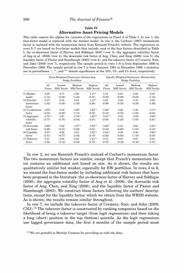
Table IVAlternative Asset Pricing Models
This table reports the alphas for variants of the regressions in Panel A of Table I. In row 1, thefour-factor model is replaced with the market model. In row 2, the Carhart (1997) momentumfactor is replaced with the momentum factor from Kenneth French’s website. The regressions inrows 3–7 are based on five-factor models that include, next to the four factors described in TableI, the co-skewness factor of Harvey and Siddique (2007) (row 3), the aggregate volatility factorof Ang et al. (2006) (row 4), the downside risk factor of Ang, Chen, and Xing (2006) (row 5), theliquidity factor of Pastor and Stambaugh (2003) (row 6), and the takeover factor of Cremers, Nair,and John (2009) (row 7), respectively. The sample period in rows 1–6 is from September 1990 toDecember 1999. The sample period in row 7 is from January 1991 to December 1999. t-statisticsare in parentheses. ∗, ∗∗, and ∗∗∗ denote significance at the 10%, 5%, and 1% level, respectively.
Value-Weighted Democracy–DictatorshipHedge Portfolios
Equally Weighted Democracy–DictatorshipHedge Portfolios
All Lowest Medium Highest All Lowest Medium HighestFirms HHI Tercile HHI Tercile HHI Tercile Firms HHI Tercile HHI Tercile HHI Tercile
[1] Market 0.48∗ 0.17 0.49 1.17∗∗ 0.15 −0.03 0.08 0.39model (1.74) (0.49) (1.34) (2.51) (0.59) (0.09) (0.25) (1.16)
[2] French’s 0.47∗ 0.10 0.61 1.13∗∗ 0.23 0.08 0.10 0.53∗
momentum (1.82) (0.29) (1.56) (2.56) (0.99) (0.23) (0.29) (1.69)factor
[3] Co-skewness 0.65∗∗ 0.30 0.65∗ 1.42∗∗∗ 0.46∗∗ 0.26 0.40 0.71∗∗
factor (2.52) (0.89) (1.74) (3.33) (2.12) (0.78) (1.23) (2.33)[4] Aggregate 0.72∗∗∗ 0.27 0.76∗∗ 1.59∗∗∗ 0.61∗∗∗ 0.42 0.59∗ 0.80∗∗
volatility (2.77) (0.78) (2.02) (3.61) (2.85) (1.25) (1.83) (2.61)factor
[5] Downside 0.69∗∗ 0.22 1.07∗∗ 1.58∗∗∗ 0.62∗∗ 0.43 0.63 0.81∗∗
risk factor (2.08) (0.51) (2.22) (2.81) (2.19) (0.99) (1.55) (2.10)[6] Liquidity 0.57∗∗ 0.26 0.61 1.32∗∗∗ 0.44∗∗ 0.28 0.36 0.68∗∗
factor (2.31) (0.77) (1.62) (3.15) (2.02) (0.83) (1.10) (2.23)[7] Takeover 0.31 −0.05 0.23 1.41∗∗∗ 0.18 −0.04 0.07 0.54
factor (1.04) (0.12) (0.50) (2.75) (0.75) (0.10) (0.19) (1.57)
In row 2, we use Kenneth French’s instead of Carhart’s momentum factor.The two momentum factors are similar, except that French’s momentum fac-tor contains an additional sort based on size. As is shown, the results arequalitatively similar but weaker, especially for EW portfolios. In rows 3 to 6,we extend the four-factor model by including additional risk factors that havebeen proposed in the literature: the co-skewness factor of Harvey and Siddique(2000), the aggregate volatility factor of Ang et al. (2006), the downside riskfactor of Ang, Chen, and Xing (2006), and the liquidity factor of Pastor andStambaugh (2003). We construct these factors following the authors’ descrip-tions, except for the liquidity factor, which we obtain from the WRDS website.As is shown, the results remain similar throughout.
In row 7, we include the takeover factor of Cremers, Nair, and John (2009,CNJ).14 The takeover factor is constructed by ranking companies based on thelikelihood of being a takeover target (from logit regressions) and then takinga long (short) position in the top (bottom) quintile. As the logit regressionsuse lagged governance data, the first 4 months of the sample period must
14 We are grateful to Martijn Cremers for providing us with the data.

Corporate Governance, Product Market Competition 581
be dropped. As CNJ point out, it is not obvious what effect the takeover fac-tor might have on GIM’s results. Although the G-index and takeover activityare clearly related, many of the provisions in the G-index are unrelated totakeovers. On the other hand, takeovers may occur for reasons unrelated togovernance, such as synergies. When CNJ estimate a five-factor model thatincludes the takeover factor as an additional risk factor, they find that theabnormal return to the Democracy–Dictatorship portfolio becomes insignifi-cant, suggesting that it is primarily driven by G-index provisions that aretakeover related. Consistent with this result, we also find that the (average)alpha based on the entire sample becomes insignificant. However, the alpharemains monotonic across HHI terciles and, at least for VW portfolios, sig-nificant in the highest HHI tercile, suggesting that the abnormal return tothe Democracy–Dictatorship portfolio is at least partly also driven by G-indexprovisions that are unrelated to takeovers.
E.2. Fama–MacBeth Return Regressions
To address concerns that the abnormal return to the Democracy–Dictatorshiphedge portfolio might be driven by an omitted variable bias, GIM estimateFama–MacBeth return regressions that include a broad array of control vari-ables. We augment GIM’s specification in two ways. First, we interact all gover-nance measures with the HHI. Second, we include additional control variables.We estimate the cross-sectional regression
rit = αt + β ′t(Git × Iit) + γ ′
tXit + εit, (2)
where rit is the return on firm i’s stock in month t, Git is either the G-indexor a Dictatorship dummy, Iit is a (3 × 1) vector of HHI dummies, and Xit isa vector of control variables. The HHI dummies indicate whether the HHI offirm i in month t lies in the lowest, medium, or highest tercile of its empiricaldistribution. All right-hand-side variables are lagged. We estimate equation (2)for each month and calculate the mean and time-series standard deviationof the 112 monthly estimates to obtain the Fama–MacBeth coefficients andstandard errors.
As elements of X, we include the full set of control variables used in GIM:firm size; book-to-market ratio; stock price; returns from months t − 3 tot − 2, from t − 6 to t − 4, and from t − 12 to t − 7; trading volume of NYSEor Amex stocks; trading volume of NASDAQ stocks; a NASDAQ dummy; anS&P 500 dummy; dividend yield; sales growth over the previous 5 years; andinstitutional ownership. A description of all these variables can be found in theAppendix of GIM. To control for any direct effect of competition, we also includeHHI dummies. Finally, we include a measure of idiosyncratic volatility. In arecent paper, Ferreira and Laux (2007, FL) show that firms with fewer anti-takeover provisions exhibit higher levels of idiosyncratic volatility. This couldhave pricing implications. Our measure of idiosyncratic volatility is the sameas in FL.

582 The Journal of Finance R©
Table VFama-MacBeth Return Regressions
This table reports the Fama-MacBeth coefficients from monthly cross-sectional regressions ofindividual stock returns on an intercept, either the G-index or a Dictatorship dummy, and controlvariables. The Dictatorship dummy equals one if a firm is a Dictatorship firm and zero otherwise.The control variables are firm size; book-to-market ratio; stock price; returns from months t − 3to t − 2, from t − 6 to t − 4, and from t − 12 to t − 7; trading volume of NYSE or Amex stocks;trading volume of NASDAQ stocks; a NASDAQ dummy; an S&P 500 dummy; dividend yield; salesgrowth over the previous 5 years; institutional ownership; and the Ferreira-Laux (2007) measureof idiosyncratic volatility. A description of all control variables (except for idiosyncratic volatility)can be found in Gompers, Ishii, and Metrick (2003). In columns 2 and 4, the G-index and theDictatorship dummy are interacted with HHI dummies indicating whether the HHI lies in thelowest, medium, or highest tercile of its empirical distribution, and HHI dummies are included asadditional control variables. All right-hand-side variables are lagged. The samples in columns 3and 4 are restricted to Democracy and Dictatorship firms. The G-index, the HHI, and Democracyand Dictatorship firms are defined in Table I. Columns 1 and 3 report the coefficients on the G-index and the Dictatorship dummy, respectively, and columns 2 and 4 report the coefficients oninteraction terms between either the G-index or the Dictatorship dummy and HHI dummies aswell as the coefficients on the HHI dummies as control variables. The coefficients on the interceptand the other control variables are not reported for brevity. The sample period is from September1990 to December 1999. t-statistics are in parentheses. ∗, ∗∗, and ∗∗∗ denote significance at the 10%,5%, and 1% level, respectively.
[1] [2] [3] [4]
G-index −0.04(1.28)
G-index × HHI (low) −0.02(0.21)
G-index × HHI (medium) −0.02(0.59)
G-index × HHI (high) −0.12∗(1.93)
Dictatorship −0.77∗∗(2.43)
Dictatorship × HHI (low) −0.24(0.60)
Dictatorship × HHI (medium) −1.00∗(1.72)
Dictatorship × HHI (high) −1.77∗∗(2.52)
HHI (medium) 0.01 0.67(0.01) (1.33)
HHI (high) 0.78 0.82(0.99) (1.64)
Number of months 112 112 112 112Number of observations 122,595 122,595 21,299 21,299
Table V shows the results. In column 1, the coefficient on the noninteractedG-index is small (−0.04) and insignificant, which is identical to the result inGIM. The outcome is markedly different if we restrict the sample to Democracyand Dictatorship firms and use a Dictatorship dummy as our governance proxy.In column 3, the coefficient on the noninteracted Dictatorship dummy is large
Corporate Governance, Product Market Competition 583
and significant (−0.77, t = 2.43), which is similar to the result in GIM (0.76,t = 2.38). (GIM use a Democracy dummy instead of a Dictatorship dummy,which implies that the sign of the coefficient is reversed.) As GIM note, thiscoefficient can be interpreted as a monthly abnormal return. Hence,the monthly abnormal return to Democracy stocks is 0.77% higher thanthe monthly abnormal return to Dictatorship stocks, which is roughlyof similar magnitude as the monthly abnormal return of 0.66% to theDemocracy–Dictatorship hedge portfolio shown in Table I. That the resultsare much stronger if we use a Dictatorship dummy as opposed to the G-indexis not surprising: as equity returns are very noisy, the effect can often only befound in the extremes. In columns 2 and 4, we find the same pattern acrossHHI terciles as before. Regardless of whether we use the G-index or a Dicta-torship dummy as our governance proxy, the coefficient is always small andinsignificant in the lowest HHI tercile, is monotonic across HHI terciles, and islarge and significant in the highest HHI tercile. Importantly, that the resultsare similar if we use a broad array of control variables mitigates concerns thatthey might be driven by an omitted variable bias.
F. Analysts’ Earnings Forecasts
There are two potential explanations for the abnormal return to theDemocracy–Dictatorship hedge portfolio. One is that the G-index is correlatedwith risk characteristics that are priced during the sample period but that arenot captured by the asset pricing model in equation (1). As is shown in theprevious section, and consistent with GIM’s own results, we find no supportfor this hypothesis. The other explanation is that weak governance gives riseto agency costs whose magnitude is underestimated by investors. Consistentwith the first part of this hypothesis, GIM find that weak governance is asso-ciated with both higher capital expenditures and higher acquisition activity.Likewise, Core et al. (2006, CGR) and GIM both find that weak governance isassociated with worse operating performance. However, CGR find no evidencefor the second part of the hypothesis, namely, that investors are surprised. Theauthors test whether the stock market underperformance of weak governancefirms is due to investor surprise about the poor operating performance of thesefirms. Using analysts’ earnings forecasts to proxy for investors’ expectations,they find no significant relationship between governance proxies and analysts’forecast errors.
Following CGR, we use analysts’ earnings forecasts to proxy for investors’expectations. Data on analysts’ earnings forecasts are obtained from the Insti-tutional Brokers’ Estimate System (I/B/E/S). Our main measure is the meanI/B/E/S consensus forecast of annual earnings per share (EPS) measured 8months prior to the fiscal year’s end. We obtain virtually identical results usingmedian I/B/E/S consensus forecasts. Measuring analysts’ forecasts 8 monthsbefore the fiscal year’s end ensures that the analysts know the previous year’searnings when making their forecasts. To mitigate the effect of outliers, we re-move observations for which the forecast error is larger than 10% of the share
584 The Journal of Finance R©
price in the month of the forecast (less than 3% of the sample) (e.g., Lim (2001),Teoh and Wong (2002)). Also, to ensure that consensus forecasts constitute re-liable proxies of market expectations, we require that a company be followedby at least five analysts (e.g., Easterwood and Nutt (1999), Loha and Mianc(2006)).
We estimate the equation
yit = α j + αt + β ′(Git−1 × Iit−1) + γ ′Xit−1 + εit, (3)
where yit is either the mean I/B/E/S consensus forecast of annual EPS, theactual I/B/E/S annual EPS, or the forecast error (difference between actual andforecasted EPS) for firm i in year t, all scaled down by lagged total assets pershare, where total assets is the book value of total assets (Compustat item #6),αj and αt are industry and year fixed effects, Git−1 is a Dictatorship dummy, Iit−1
is a (3 × 1) vector of HHI dummies, and Xit−1 is a vector of control variables.All right-hand-side variables are lagged. As control variables, we include HHIdummies, the book-to-market ratio, and firm size. Firm size is the logarithmof the book value of total assets. The book-to-market ratio is computed as thelogarithm of the ratio of the book value of equity (item #60 + item #74) dividedby the market value of equity (item #199 × item #25). The sample is restrictedto Democracy and Dictatorship firms. The sample period is from 1991 to 1999.Standard errors are clustered at the industry level.15
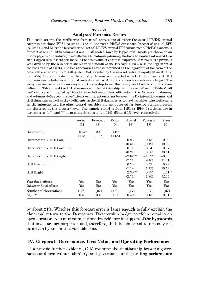
Table VI shows the results. (Robustness checks can be found in the InternetAppendix.) Columns 1 and 2 show that Dictatorship firms exhibit on aver-age lower EPS than Democracy firms and that analysts correctly predict thisoutcome. The forecast error, which is shown in column 3, is small and insignif-icant. Based on this evidence, CGR conclude that investors are not surprised.However, columns 4 to 6 paint a more nuanced picture. Column 4 shows thatDictatorship firms exhibit lower EPS only in noncompetitive industries (high-est HHI tercile). Remarkably, analysts correctly predict this outcome: in column5, the difference in forecasted EPS between Dictatorship and Democracy firmsis significant only in the highest HHI tercile, while it is otherwise small andinsignificant. Importantly, however, while analysts correctly predict that gover-nance matters for EPS only in noncompetitive industries, they underestimatethe magnitude of this effect: in column 6, the forecast error in the highest HHItercile is large (−0.43) and significant (p = 0.07). Thus, analysts underestimatethe effect of governance on earnings in precisely those industries in which gov-ernance matters for earnings, namely, noncompetitive industries. The economicmagnitude of the forecast error is large: in the highest HHI tercile, analysts un-derestimate the difference in EPS between Dictatorship and Democracy firms
15 CGR use the Fama–MacBeth method while accounting for serial correlation using theNewey–West procedure with one lag. However, when the dependent and independent variablesare both persistent, the Fama–MacBeth method produces biased standard errors even if combinedwith the Newey–West procedure (Petersen (2009)). To avoid this bias, we estimate a panel regres-sion with fixed effects and clustered standard errors. The choice of industry rather than firm fixedeffects is due to insufficient within-variation of the G-index.
Corporate Governance, Product Market Competition 585
Table VIAnalysts’ Forecast Errors
This table reports the coefficients from panel regressions of either the actual I/B/E/S annualearnings per share (EPS) (columns 1 and 4), the mean I/B/E/S consensus forecast of annual EPS(columns 2 and 5), or the forecast error (actual I/B/E/S annual EPS minus mean I/B/E/S consensusforecast of annual EPS; columns 3 and 6), all scaled down by lagged total assets per share, on anintercept, year and industry fixed effects, a Dictatorship dummy, the book-to-market ratio, and firmsize. Lagged total assets per share is the book value of assets (Compustat item #6) in the previousyear divided by the number of shares in the month of the forecast. Firm size is the logarithm ofthe book value of assets. The book-to-market ratio is computed as the logarithm of the ratio of thebook value of equity (item #60 + item #74) divided by the market value of equity (item #199 ×item #25). In columns 4–6, the Dictatorship dummy is interacted with HHI dummies, and HHIdummies are included as additional control variables. All right-hand-side variables are lagged. Thesample is restricted to Democracy and Dictatorship firms. Democracy and Dictatorship firms aredefined in Table I, and the HHI dummies and the Dictatorship dummy are defined in Table V. Allcoefficients are multiplied by 100. Columns 1–3 report the coefficients on the Dictatorship dummy,and columns 4–6 report the coefficients on interaction terms between the Dictatorship dummy andHHI dummies as well as the coefficients on the HHI dummies as control variables. The coefficientson the intercept and the other control variables are not reported for brevity. Standard errorsare clustered at the industry level. The sample period is from 1991 to 1999. t-statistics are inparentheses. ∗, ∗∗, and ∗∗∗ denotes significance at the 10%, 5%, and 1% level, respectively.
Actual Forecast Error Actual Forecast Error[1] [2] [3] [4] [5] [6]
Dictatorship −0.57∗ −0.48 −0.09(1.66) (1.25) (0.68)
Dictatorship × HHI (low) 0.23 0.13 0.10(0.31) (0.19) (0.72)
Dictatorship × HHI (medium) 0.11 0.04 0.07(0.21) (0.08) (0.31)
Dictatorship × HHI (high) −2.02∗∗∗ −1.59∗∗ −0.43∗(2.71) (2.16) (1.81)
HHI (medium) 0.79 0.57 0.22(1.14) (1.12) (0.59)
HHI (high) 2.30∗∗∗ 0.99∗ 1.31∗∗(2.71) (1.70) (2.15)
Year fixed effects Yes Yes Yes Yes Yes YesIndustry fixed effects Yes Yes Yes Yes Yes Yes
Number of observations 1,071 1,071 1,071 1,071 1,071 1,071Adj. R2 0.40 0.43 0.11 0.40 0.43 0.11
by about 21%. Whether this forecast error is large enough to fully explain theabnormal return to the Democracy–Dictatorship hedge portfolio remains anopen question. At a minimum, it provides evidence in support of the hypothesisthat investors are surprised and, therefore, that the abnormal return may notbe driven by an omitted variable bias.
IV. Corporate Governance, Firm Value, and Operating Performance
To provide further evidence, GIM examine the relationship between gover-nance and firm value (Tobin’s Q) and governance and operating performance

586 The Journal of Finance R©
(net profit margin, ROE, sales growth). Core et al. (2006) extend GIM’s resultsby examining the relationship between governance and return on assets (ROA).In this section, we examine whether any of these relationships are different incompetitive versus noncompetitive industries.
A. Corporate Governance and Firm Value
To examine the relationship between governance and firm value, we estimate
Q∗it = α j + αt + β ′ (Git × Iit) + γ ′Xit + εit, (4)
where Q∗it is the industry-adjusted Tobin’s Q of firm i in year t, Git is the
G-index, Iit is a (3 × 1) vector of HHI dummies, αj and αt are industry andyear fixed effects, and Xit is a vector of control variables. The choice of industryrather than firm fixed effects is due to insufficient within-variation of the G-index, a point that has already been made by GIM (p. 126). Tobin’s Q is themarket value of assets divided by the book value of assets (Compustat item #6),where the market value of assets is the book value of assets plus the marketvalue of common stock (item #24 ×item #25) minus the sum of the book value ofcommon stock (item #60) and balance sheet deferred taxes (item #74). Industry-adjusted Tobin’s Q is computed by subtracting the industry median in a given48 FF industry and year. Industry medians are computed using all availableCompustat firms. As elements of X, we include the full set of control variablesused in GIM: firm size, which is the logarithm of the book value of assets,firm age (in logs), an S&P 500 dummy, and a Delaware dummy. To control forany direct effect of competition on firm value, we also include HHI dummies.Standard errors are clustered at the industry level. The sample period is from1990 to 2006.
Table VII presents the results.16 (Robustness checks can be found in theInternet Appendix.) In column 1, the coefficient on the noninteracted G-indexis −0.036 (t = 3.46), implying that an increase in the G-index by one index pointis associated with a 3.6% lower value for Tobin’s Q. In column 2, we obtain thesame pattern across HHI terciles as before: the coefficient on the G-index issmall (−0.005) and insignificant in the lowest HHI tercile, is larger (−0.043)and significant (t = 1.77) in the medium HHI tercile, and is largest (−0.065)and significant (t = 3.17) in the highest HHI tercile.
B. Corporate Governance and Operating Performance
To examine the relationship between governance and operating performance,we use the same specification as in equation (4), except that the dependent
16 We obtain similar results if we use median (least absolute deviation) regressions instead ofOLS. We also obtain similar results if we estimate year-by-year cross-sectional regressions. Forthe years 1990 to 2006, the coefficient on the G-index is small and insignificant in the lowest HHItercile in all years, is monotonic across HHI terciles in most years (12 out of 17 years), and isalways large and almost always (16 out of 17 years) significant in the highest HHI tercile (see theInternet Appendix).

Corporate Governance, Product Market Competition 587
Table VIITobin’s Q
This table reports the coefficients from panel regressions of industry-adjusted Tobin’s Q on anintercept, year and industry fixed effects, the G-index, firm size, firm age, an S&P 500 dummy,and a Delaware dummy. A description of all control variables can be found in Gompers, Ishii,and Metrick (2003). Tobin’s Q is the market value of assets divided by the book value of assets(Compustat item #6), where the market value of assets is the book value of assets plus the marketvalue of common stock (item #24 × item #25) minus the sum of the book value of common stock(item #60) and balance sheet deferred taxes (item #74). Industry-adjusted Tobin’s Q is computedby subtracting the industry median in a given 48 FF industry and year. Industry medians arecomputed using all available Compustat firms. In column 2, the G-index is interacted with HHIdummies, and HHI dummies are included as additional control variables. The G-index is definedin Table I, and the HHI dummies are defined in Table V. Column 1 reports the coefficient on theG-index, and column 2 reports the coefficients on interaction terms between the G-index and HHIdummies as well as the coefficients on the HHI dummies as control variables. The coefficients on theintercept and the other control variables are not reported for brevity. Standard errors are clusteredat the industry level. The sample period is from 1990 to 2006. t-statistics are in parentheses. ∗, ∗∗,and ∗∗∗ denotes significance at the 10%, 5%, and 1% level, respectively.
[1] [2]
G-index −0.036∗∗∗(3.46)
G-index × HHI (low) −0.005(0.33)
G-index × HHI (medium) −0.043∗(1.77)
G-index × HHI (high) −0.065∗∗∗(3.17)
HHI (medium) 0.463(1.42)
HHI (high) 0.671∗∗(2.40)
Year fixed effects Yes YesIndustry fixed effects Yes Yes
Number of observations 20,051 20,051Adj. R2 0.08 0.08
variable is now either ROA, net profit margin (NPM), sales growth, or ROE.ROA is net income (Compustat item #172) divided by the book value of totalassets (item #6), NPM is net income divided by sales (item #12), sales growthis the growth in sales over the previous 5 years, and ROE is net income dividedby the book value of common stock (item #60). Following GIM, we include thelogarithm of the book-to-market ratio in the previous year as an additionalcontrol variable. The book-to-market ratio is computed as the ratio of the bookvalue of common stock plus balance sheet deferred taxes (item #74) dividedby the market value of common stock (item #24 × item #25). All dependentvariables are industry-adjusted by subtracting the industry median in a given48 FF industry and year. Industry medians are computed using all availableCompustat firms. To account for outliers, we trim all dependent variables at

588 The Journal of Finance R©
Table VIIIOperating Performance
This table reports the coefficients from panel regressions of industry-adjusted measures of operat-ing performance on an intercept, year and industry fixed effects, the G-index, and control variables.The control variables are the same as in Table VII plus the logarithm of the book-to-market ratio inthe previous year. The book-to-market ratio is computed as the ratio of the book value of commonstock (Compustat item #60) plus balance sheet deferred taxes (item #74) divided by the marketvalue of common stock (item #24 × item #25). In columns 2, 4, 6, and 8, the G-index is interactedwith HHI dummies, and HHI dummies are included as additional control variables. The G-indexand the HHI dummies are defined in Tables I and V, respectively. All right-hand-side variables arelagged. In columns 1 and 2, the dependent variable is return on assets (ROA), which is net income(item #172) divided by the book value of assets (item #6). In columns 3 and 4, the dependent vari-able is net profit margin (NPM), which is net income divided by sales (item #12). In columns 5 and6, the dependent variable is sales growth, which is the growth in sales over the previous 5 years.In columns 7 and 8, the dependent variable is return on equity (ROE), which is net income dividedby the book value of common stock. All dependent variables are industry-adjusted by subtractingthe industry median in a given 48 FF industry and year. Industry medians are computed using allavailable Compustat firms. All dependent variables are trimmed at the 5th and 95th percentilesof their empirical distributions. In columns 1–4 and 7–8, the coefficients are multiplied by 100,and in columns 5 and 6, they are multiplied by 10. Columns 1, 3, 5, and 7 report the coefficient onthe G-index, and columns 2, 4, 6, and 8 report the coefficients on interaction terms between theG-index and HHI dummies as well as the coefficients on the HHI dummies as control variables. Thecoefficients on the intercept and the other control variables are not reported for brevity. Standarderrors are clustered at the industry level. The sample period is from 1990 to 2006. t-statistics arein parentheses. ∗, ∗∗, and ∗∗∗ denotes significance at the 10%, 5%, and 1% level, respectively.
ROA NPM Sales Growth ROE
[1] [2] [3] [4] [5] [6] [7] [8]
G-index −0.066∗∗∗ −0.108∗∗∗ −0.064∗∗ −0.010(2.88) (3.47) (2.35) (0.30)
G-index × −0.001 −0.011 −0.004 0.054HHI (low) (0.02) (0.21) (0.07) (0.87)
G-index × −0.076∗∗ −0.139∗∗ −0.096∗∗∗ −0.004HHI (medium) (2.02) (2.14) (2.65) (0.05)
G-index × −0.137∗∗∗ −0.192∗∗∗ −0.109∗∗∗ −0.099∗HHI (high) (4.34) (2.87) (3.06) (1.93)
HHI (medium) 0.877 1.518 1.414∗∗ 0.771(1.48) (1.21) (2.05) (0.65)
HHI (high) 1.051∗ 1.633∗ 1.975∗∗∗ 1.926∗(1.75) (1.87) (2.72) (1.74)
Year fixed Yes Yes Yes Yes Yes Yes Yes Yeseffects
Year fixed Yes Yes Yes Yes Yes Yes Yes Yeseffects
Number of 17,699 17,699 17,699 17,699 17,699 17,699 17,699 17,699observations
Adj. R2 0.32 0.32 0.23 0.23 0.24 0.24 0.24 0.24
the 5th and 95th percentiles of their empirical distribution. We obtain similarresults if we use different cutoffs, or if we use median regressions instead. Allright-hand variables are lagged. The sample period is from 1990 to 2006.
Table VIII presents the results. (Robustness checks can be found in theInternet Appendix.) In columns 1 and 2, the dependent variable is ROA.The coefficient on the noninteracted G-index is −0.066 (t = 2.88), implyingthat weak governance firms have on average lower operating performance.The pattern across HHI terciles is the same as before. The coefficient on the

Corporate Governance, Product Market Competition 589
G-index is small (−0.001) and insignificant in the lowest HHI tercile, is larger(−0.076) and significant (t = 2.02) in the medium HHI tercile, and is largest(−0.137) and significant (t = 4.34) in the highest HHI tercile.
In columns 3 to 6, the dependent variable is either NPM or sales growth.The results are similar to our ROA results. In both cases, the coefficient on thenoninteracted G-index is negative and significant, implying that weak gover-nance firms have on average lower net profit margins and lower sales growth.Moreover, the coefficient on the G-index is always small and insignificant inthe lowest HHI tercile, is monotonic across HHI terciles, and is large and sig-nificant in the highest HHI tercile. In columns 7 and 8, the dependent variableis ROE. Although the results are again similar, they are much weaker. In par-ticular, the coefficient on the noninteracted G-index is small and insignificant,which is also what GIM find for the years 1990 to 1999. Importantly, however,the coefficient on the G-index is again monotonic across HHI terciles, and it isagain large and significant in the highest HHI tercile.
V. Agency Costs of Weak Corporate Governance
Our firm value and operating performance results suggest that, absent com-petitive pressure from the product market, weak governance gives rise toagency costs. To gain a better understanding of the nature of these agencycosts, we now explore in more detail the relationship between (i) governanceand investment activity and (ii) governance and productive efficiency.
A. Capital Expenditures and Acquisition Activity
To examine the relationship between governance and investment activity,we use the same specification as in our operating performance regressions,except that the dependent variable is now either capital expenditures or somemeasure of acquisition activity. The sample period is again from 1990 to 2006.
Table IX shows the results. In columns 1 and 2, the dependent variable is cap-ital expenditures (Compustat item #30) divided by total assets (item #6). Thedependent variable is industry-adjusted by subtracting the industry medianin a given 48 FF industry and year. Industry medians are computed using allavailable Compustat firms. To account for outliers, we trim the dependent vari-able at the 5th and 95th percentiles of its empirical distribution. As is shown,the coefficient on the noninteracted G-index is positive and significant, imply-ing that weak governance firms have on average higher capital expenditures.Moreover, the coefficient on the G-index is small and insignificant in the lowestHHI tercile, is monotonic across HHI terciles, and is large and significant inthe highest HHI tercile.
Capital expenditures may be a poor measure of investment activity if mostof the activity comes in the form of acquisitions. To examine the relationshipbetween governance and acquisitions, we construct various proxies for acquisi-tion activity using data from the Securities Data Corporation’s (SDC) database.In columns 3 and 4, the dependent variable is the sum of the value of all

590 The Journal of Finance R©
Tab
leIX
Cap
ital
Exp
end
itu
res
and
Acq
uis
itio
nA
ctiv
ity
Th
ista
ble
repo
rts
the
coef
fici
ents
from
pan
elre
gres
sion
sof
eith
erca
pita
lex
pen
ditu
res
orso
me
mea
sure
ofac
quis
itio
nac
tivi
tyon
anin
terc
ept,
year
and
indu
stry
fixe
def
fect
s,th
eG
-in
dex,
and
con
trol
vari
able
s.T
he
con
trol
vari
able
sar
eth
esa
me
asin
Tab
leV
III.
Inco
lum
ns
2,4,
6,8,
and
10,t
he
G-i
nde
xis
inte
ract
edw
ith
HH
Idu
mm
ies,
and
HH
Idu
mm
ies
are
incl
ude
das
addi
tion
alco
ntr
olva
riab
les.
Th
eG
-in
dex
and
the
HH
Idu
mm
ies
are
defi
ned
inT
able
sI
and
V,r
espe
ctiv
ely.
All
righ
t-h
and-
side
vari
able
sar
ela
gged
.In
colu
mn
s1
and
2,th
ede
pen
den
tva
riab
leis
capi
tal
expe
ndi
ture
s(C
apex
;C
ompu
stat
item
#30)
divi
ded
byto
tal
asse
ts(i
tem
#6).
Cap
exis
trim
med
atth
e5th
and
95th
perc
enti
les
ofit
sem
piri
cal
dist
ribu
tion
and
isin
dust
ry-a
dju
sted
bysu
btra
ctin
gth
ein
dust
rym
edia
nin
agi
ven
48F
Fin
dust
ryan
dye
ar.
Indu
stry
med
ian
sar
eco
mpu
ted
usi
ng
all
avai
labl
eC
ompu
stat
firm
s.In
colu
mn
s3
and
4,th
ede
pen
den
tva
riab
leis
the
acqu
isit
ion
rati
o,w
hic
his
the
sum
ofth
eva
lue
ofal
lacq
uis
itio
ns
mad
eby
afi
rmin
agi
ven
year
divi
ded
byth
efi
rm’s
aver
age
mar
ket
capi
tali
zati
onin
that
year
.In
colu
mn
s5
and
6,th
ede
pen
den
tva
riab
leis
the
acqu
isit
ion
cou
nt,
wh
ich
isth
en
um
ber
ofac
quis
itio
ns
mad
eby
afi
rmin
agi
ven
year
.In
colu
mn
s7
and
8,th
ede
pen
den
tva
riab
leis
the
acqu
isit
ion
like
lih
ood,
wh
ich
isa
dum
my
vari
able
that
equ
als
one
ifth
efi
rmm
akes
atle
ast
one
acqu
isit
ion
duri
ng
the
year
and
zero
oth
erw
ise.
Inco
lum
ns
9an
d10
,th
ede
pen
den
tva
riab
leis
CA
R(−
2,+2
),w
hic
his
the
acqu
irin
gfi
rm’s
5-da
ycu
mu
lati
veab
nor
mal
retu
rn(C
AR
)ar
oun
dth
eac
quis
itio
nan
nou
nce
men
t.C
AR
sar
eco
mpu
ted
byes
tim
atin
gth
epa
ram
eter
sof
the
mar
ket
mod
elov
era
200-
day
peri
odfr
omev
ent
day
−210
toev
ent
day
−11,
wh
ere
the
CR
SP
equ
ally
wei
ghte
dre
turn
isu
sed
asth
em
arke
tre
turn
.Col
um
ns
3an
d4
are
base
don
Tobi
tre
gres
sion
s,co
lum
ns
5an
d6
are
base
don
Poi
sson
regr
essi
ons,
and
colu
mn
s7
and
8ar
eba
sed
onP
robi
tre
gres
sion
s.In
colu
mn
s3–
8,th
eR
2is
McF
adde
n’s
pseu
doR
2.A
llco
effi
cien
tsar
em
ult
ipli
edby
100.
Col
um
ns
1,3,
5,7,
and
9re
port
the
coef
fici
ent
onth
eG
-in
dex,
and
colu
mn
s2,
4,6,
8,an
d10
repo
rtth
eco
effi
cien
tson
inte
ract
ion
term
sbe
twee
nth
eG
-in
dex
and
HH
Idu
mm
ies
asw
ella
sth
eco
effi
cien
tson
the
HH
Idu
mm
ies
asco
ntr
olva
riab
les.
Th
eco
effi
cien
tson
the
inte
rcep
tan
dth
eot
her
con
trol
vari
able
sar
en
otre
port
edfo
rbr
evit
y.S
tan
dard
erro
rsar
ecl
ust
ered
atth
ein
dust
ryle
vel.
Th
esa
mpl
epe
riod
isfr
om19
90to
2006
.t-s
tati
stic
sar
ein
pare
nth
eses
.∗ ,
∗∗,a
nd
∗∗∗
den
otes
sign
ifica
nce
atth
e10
%,5
%,a
nd
1%le
vel,
resp
ecti
vely
.
Cap
exA
cqu
isit
ion
Rat
ioA
cqu
isit
ion
Cou
nt
Acq
uis
itio
nL
ikel
ihoo
dC
AR
(−2,
+2)
[1]
[2]
[3]
[4]
[5]
[6]
[7]
[8]
[9]
[10]
G-i
nde
x0.
032∗
∗1.
176∗
∗∗3.
449∗
∗∗2.
256∗
∗∗−0
.074
∗(2
.35)
(4.3
8)(3
.78)
(4.4
8)(1
.67)
G-i
nde
x×
0.01
90.
895
1.65
91.
362
−0.0
60H
HI
(low
)(0
.96)
(1.5
9)(0
.91)
(0.9
8)(0
.78)
G-i
nde
x×
0.02
51.
157∗
∗4.
008∗
∗2.
603∗
∗−0
.043
HH
I(m
ediu
m)
(0.9
7)(2
.04)
(2.5
4)(2
.00)
(0.4
4)G
-in
dex
×0.
053∗
∗1.
495∗
∗4.
557∗
∗2.
832∗
∗−0
.124
∗H
HI
(hig
h)
(2.0
8)(2
.51)
(2.3
0)(2
.26)
(1.7
4)
(con
tin
ued
)

Corporate Governance, Product Market Competition 591
Tab
leIX
—C
onti
nu
ed
Cap
exA
cqu
isit
ion
Rat
ioA
cqu
isit
ion
Cou
nt
Acq
uis
itio
nL
ikel
ihoo
dC
AR
(−2,
+2)
[1]
[2]
[3]
[4]
[5]
[6]
[7]
[8]
[9]
[10]
HH
I(m
ediu
m)
0.08
3−4
.457
−2.9
80−0
.151
0.07
4(0
.19)
(0.4
8)(1
.09)
(0.6
3)(0
.07)
HH
I(h
igh
)−0
.171
−5.6
24−2
.524
−0.1
480.
801
(0.4
4)(0
.96)
(1.2
2)(0
.97)
(0.7
8)Ye
arfi
xed
Yes
Yes
Yes
Yes
Yes
Yes
Yes
Yes
Yes
Yes
effe
cts
Indu
stry
fixe
dYe
sYe
sYe
sYe
sYe
sYe
sYe
sYe
sYe
sYe
sef
fect
sR
egre
ssio
nty
peO
LS
OL
STo
bit
Tobi
tP
oiss
onP
oiss
onP
robi
tP
robi
tO
LS
OL
S
Nu
mbe
rof
17,3
5517
,355
20,2
0820
,208
20,2
0820
,208
20,2
0820
,208
4,42
64,
426
obse
rvat
ion
sA
dj./p
seu
doR
20.
080.
080.
050.
050.
050.
050.
050.
050.
020.
02

592 The Journal of Finance R©
acquisitions made by a firm in a given year divided by the firm’s average mar-ket capitalization in that year (“acquisition ratio”). In columns 5 and 6, thedependent variable is the number of acquisitions made by a firm in a givenyear (“acquisition count”). In columns 7 and 8, the dependent variable is thelikelihood of making an acquisition, which is a dummy variable that equals oneif the firm makes at least one acquisition during the year and zero otherwise.Regardless of which proxy we use, we always obtain the same result: the coeffi-cient on the noninteracted G-index is always positive and significant, implyingthat weak governance firms make on average more acquisitions. Moreover,and importantly, the coefficient on the G-index is always small and insignifi-cant in the lowest HHI tercile, is monotonic across HHI terciles, and is largeand significant in the highest HHI tercile.
That weak governance firms make more acquisitions does not necessarilyimply that these firms destroy value. However, in a recent article, Masulis et al.(2007, MWX) show that high G-index acquirer firms experience significantlylower CARs around acquisition announcements than do low G-index acquirerfirms. This result is noteworthy for two reasons. First, it suggests that weakgovernance firms make more value-destroying acquisitions. Second, becauseCARs measure unexpected changes in stock prices, the result also suggeststhat the market does not fully anticipate the negative valuation effects of weakgovernance. As MWX point out, their result is inconsistent with the argumentof Core et al. (2006) that investors are not surprised and that, consequently,the abnormal return to the Democracy–Dictatorship hedge portfolio is likelydriven by an omitted variable bias.17
For our purpose, the main question of interest is whether weak governancefirms experience significantly lower CARs only in noncompetitive industries.To address this question, we consider all acquisitions made between January 1,1990 and December 31, 2006. The acquisition data are from the SDC database.Using MWX’s selection criteria (p. 1855), this leaves us with a total of 4,426acquisitions. Our methodology is the same as in MWX. For each acquisition,we compute the 5-day bidder CAR during the event window (−2, +2), whereevent day 0 is the announcement date of the acquisition. To compute abnormalreturns, we use the CRSP EW return as the market return and estimate theparameters of the market model from day −210 to day −11 before the eventdate.
Columns 9 and 10 of Table IX present the results. The coefficient on thenoninteracted G-index is −0.074 (t = 1.67), implying that an increase in theG-index by one index point reduces acquirer shareholder wealth by 0.74%.Although this is slightly less than what MWX find (−0.096, t = 2.22), thediscrepancy is likely due to differences in the sample period and the controlvariables. MWX consider the period from 1990 to 2003, while we consider theperiod from 1990 to 2006. In addition, MWX control for a large number of
17 See MWX (pp. 1883–1884) for a discussion as well as Section III.F of this paper for furtherevidence that investors are negatively surprised about the poor operating performance of weakgovernance firms.

Corporate Governance, Product Market Competition 593
industry and deal characteristics, while we use the same specification as in ouroperating performance regressions. Importantly, however, the coefficient onthe G-index is large (−0.124) and significant (t = 1.74) only in the highest HHItercile, while it is otherwise small and insignificant. Thus, weak governancefirms make more value-destroying acquisitions, but only in noncompetitiveindustries.
B. Labor Productivity and Cost Efficiency
An alternative hypothesis is that managers of poorly governed firms en-joy the “quiet life” by avoiding “cognitively difficult activities” (Bertrand andMullainathan (2003)), such as fighting with labor unions, haggling with in-put suppliers, and expending effort to improve labor productivity. To explorethis hypothesis, we again use the same specification as in our operating per-formance regressions, except that the dependent variable is now either laborproductivity or some measure of cost efficiency. All dependent variables areindustry-adjusted by subtracting the industry median in a given 48 FF indus-try and year. Industry medians are computed using all available Compustatfirms. To account for outliers, we trim all dependent variables at the 5th and95th percentiles of their empirical distribution. All right-hand variables arelagged. The sample period is again from 1990 to 2006.
Table X presents the results. In columns 1 and 2, the dependent variableis labor productivity, which is the logarithm of sales (Compustat item #12)divided by the number of employees (item #29) and deflated by the consumerprice index from the U.S. Bureau of Labor Statistics. In columns 3 and 4, thedependent variable is costs of goods sold (item #41, “input costs”) divided bysales. In both cases, we find similar results. The coefficient on the noninteractedG-index is either negative and significant (labor productivity) or positive andsignificant (input costs), implying that weak governance firms have on averagelower labor productivity and higher input costs. Moreover, the coefficient onthe G-index is small and insignificant in the lowest HHI tercile, is monotonicacross HHI terciles, and is large and significant in the highest HHI tercile.
In columns 5 and 6, the dependent variable is real wages, which is thelogarithm of labor and related expenses (item #42) divided by the number ofemployees and deflated by the consumer price index. Although the results arequalitatively similar, they are much weaker. In particular, the coefficient onthe noninteracted G-index, although positive, is insignificant (t = 1.61). Also,the coefficient on the G-index in the highest HHI tercile, while almost twice aslarge as the coefficient in the lowest HHI tercile, is not significant (t = 1.42).That the results are weaker is not entirely surprising. Compustat wage dataare extremely spotty. While some firms report wage data only intermittently,others report no wage data at all (see Bertrand and Mullainathan (1999)). Asa consequence, the sample is considerably smaller and, furthermore, it is verynoisy, making statistical inferences difficult.
In columns 7 and 8, the dependent variable is selling, general, and admin-istrative expenses (item #189, “overhead costs”) divided by total assets (item
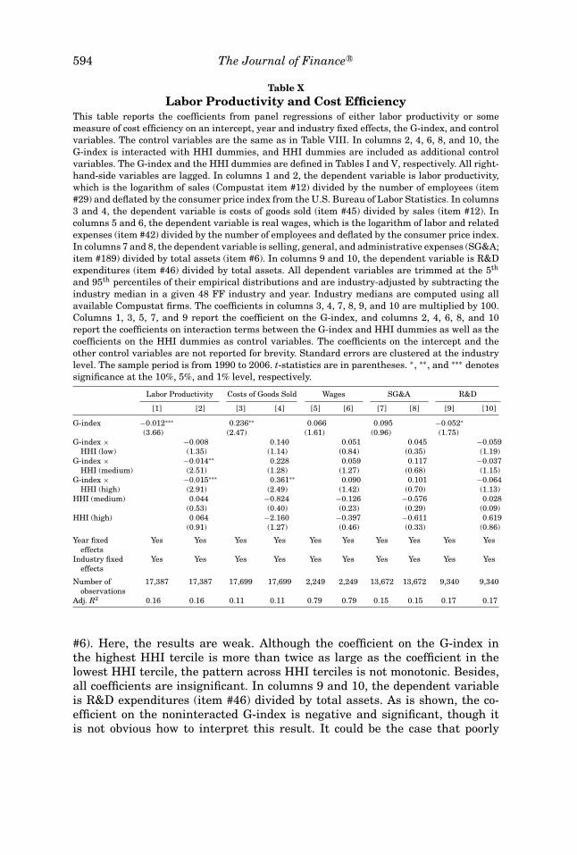
594 The Journal of Finance R©
Table XLabor Productivity and Cost Efficiency
This table reports the coefficients from panel regressions of either labor productivity or somemeasure of cost efficiency on an intercept, year and industry fixed effects, the G-index, and controlvariables. The control variables are the same as in Table VIII. In columns 2, 4, 6, 8, and 10, theG-index is interacted with HHI dummies, and HHI dummies are included as additional controlvariables. The G-index and the HHI dummies are defined in Tables I and V, respectively. All right-hand-side variables are lagged. In columns 1 and 2, the dependent variable is labor productivity,which is the logarithm of sales (Compustat item #12) divided by the number of employees (item#29) and deflated by the consumer price index from the U.S. Bureau of Labor Statistics. In columns3 and 4, the dependent variable is costs of goods sold (item #45) divided by sales (item #12). Incolumns 5 and 6, the dependent variable is real wages, which is the logarithm of labor and relatedexpenses (item #42) divided by the number of employees and deflated by the consumer price index.In columns 7 and 8, the dependent variable is selling, general, and administrative expenses (SG&A;item #189) divided by total assets (item #6). In columns 9 and 10, the dependent variable is R&Dexpenditures (item #46) divided by total assets. All dependent variables are trimmed at the 5th
and 95th percentiles of their empirical distributions and are industry-adjusted by subtracting theindustry median in a given 48 FF industry and year. Industry medians are computed using allavailable Compustat firms. The coefficients in columns 3, 4, 7, 8, 9, and 10 are multiplied by 100.Columns 1, 3, 5, 7, and 9 report the coefficient on the G-index, and columns 2, 4, 6, 8, and 10report the coefficients on interaction terms between the G-index and HHI dummies as well as thecoefficients on the HHI dummies as control variables. The coefficients on the intercept and theother control variables are not reported for brevity. Standard errors are clustered at the industrylevel. The sample period is from 1990 to 2006. t-statistics are in parentheses. ∗, ∗∗, and ∗∗∗ denotessignificance at the 10%, 5%, and 1% level, respectively.
Labor Productivity Costs of Goods Sold Wages SG&A R&D
[1] [2] [3] [4] [5] [6] [7] [8] [9] [10]
G-index −0.012∗∗∗ 0.236∗∗ 0.066 0.095 −0.052∗
(3.66) (2.47) (1.61) (0.96) (1.75)G-index × −0.008 0.140 0.051 0.045 −0.059
HHI (low) (1.35) (1.14) (0.84) (0.35) (1.19)G-index × −0.014∗∗ 0.228 0.059 0.117 −0.037
HHI (medium) (2.51) (1.28) (1.27) (0.68) (1.15)G-index × −0.015∗∗∗ 0.361∗∗ 0.090 0.101 −0.064
HHI (high) (2.91) (2.49) (1.42) (0.70) (1.13)HHI (medium) 0.044 −0.824 −0.126 −0.576 0.028
(0.53) (0.40) (0.23) (0.29) (0.09)HHI (high) 0.064 −2.160 −0.397 −0.611 0.619
(0.91) (1.27) (0.46) (0.33) (0.86)
Year fixed Yes Yes Yes Yes Yes Yes Yes Yes Yes Yeseffects
Industry fixed Yes Yes Yes Yes Yes Yes Yes Yes Yes Yeseffects
Number of 17,387 17,387 17,699 17,699 2,249 2,249 13,672 13,672 9,340 9,340observations
Adj. R2 0.16 0.16 0.11 0.11 0.79 0.79 0.15 0.15 0.17 0.17
#6). Here, the results are weak. Although the coefficient on the G-index inthe highest HHI tercile is more than twice as large as the coefficient in thelowest HHI tercile, the pattern across HHI terciles is not monotonic. Besides,all coefficients are insignificant. In columns 9 and 10, the dependent variableis R&D expenditures (item #46) divided by total assets. As is shown, the co-efficient on the noninteracted G-index is negative and significant, though itis not obvious how to interpret this result. It could be the case that poorly

Corporate Governance, Product Market Competition 595
monitored managers reduce R&D as a means to reduce their risk exposure. Orit could simply be the case that poorly monitored managers place less value onresearch. Moreover, there is no systematic pattern across HHI terciles.
VI. Hedge Fund Activism
Our results suggest that weak governance firms have lower equity returns,worse operating performance, and lower firm value, but only in noncompetitiveindustries. In this final part of our analysis, we examine whether investors takeactions to mitigate the inefficiency. In particular, we examine whether weakgovernance firms, especially those in noncompetitive industries, are more likelyto be targeted by activist hedge funds.
Early studies of shareholder activism typically focus on the activist role ofinstitutional investors, such as pension funds and mutual funds. These studiesfind little evidence that institutional investors bring about significant improve-ments in the companies they target (see Gillan and Starks (2007) for a review).More recent studies suggest that the opposite is true of activist hedge funds(Brav et al. (2008), Klein and Zur (2009)).18 For instance, Brav et al. (2008)find that in the 2 years following an intervention by an activist hedge fund,the targeted company’s ROA increases by 0.9 to 1.5 percentage points, and itsoperating profit margin increases by 4.7 to 5.8 percentage points.
To address whether weak governance firms, especially those in noncompeti-tive industries, are more likely to be targeted by activist hedge funds, we usethe data by Brav et al. (2008). The data are based on Schedule 13D filings,which investors must file with the SEC within 10 days of acquiring more than5% of any class of securities of a publicly traded company if they have an inter-est in influencing the company’s management. The data include 1,059 hedgefund interventions from 2001 to 2006 involving 882 unique target companies.To examine the likelihood that a company is targeted by an activist hedge fundin the following year, we match the data with the merged Compustat/IRRCsample from 2000 to 2005. After removing firms with dual-class shares andmissing SIC codes, the merged Compustat/IRRC sample during this periodconsists of 10,134 firm-year observations, of which 217 (or 2.14%) correspondto firms targeted by an activist hedge fund in the following year.
To examine how the likelihood of being targeted by activist hedge funds de-pends jointly on governance and competition, we sort firms into two governancegroups based on whether the G-index lies above or below the median. We thendivide each governance group into three equal-sized groups by ranking firmsaccording to their HHIs and then sorting them into HHI terciles. Similar towhat we did in our main analysis (see the Internet Appendix), we verify thatour results are not driven by systematic differences in the HHI across the twogovernance groups. As Panel A of Table XI shows, the empirical distribution
18 Brav et al. (2008) mention collective action problems, regulatory constraints, conflicts of in-terest, political constraints, and weak financial incentives as the main reasons why activist insti-tutional investors, but not activist hedge funds, are unsuccessful at implementing their objectives.

596 The Journal of Finance R©
Table XIHedge Fund Activism
Panel A sorts firms with above- and below-median G-index, respectively, into terciles based ontheir HHIs. For each HHI tercile, it shows the mean HHI, median HHI, and range of observedHHI values. The sample period is from 2000 to 2005. The G-index and the HHI are defined inTable I. Panel B shows the percentage of firms targeted by an activist hedge fund in the followingyear for each of the 2 × 3 = 6 groups from Panel A. The sample consists of 10,134 firm-yearobservations from 2000 to 2005, of which 217 observations correspond to firms targeted by anactivist hedge fund in the following year. Panel C shows the change in the G-index following ahedge fund intervention for 127 interventions between 2000 and 2005. The change in the G-indexis computed as the difference between the G-index published in the next available IRRC file afterthe intervention and the G-index published in the latest IRRC file prior to the intervention. (As thelast IRRC file was published in January 2006, interventions in 2006 are excluded.) It is adjustedfor general trends in the G-index by subtracting the average change in the G-index during thesame time period based on all firms in the IRRC sample. In Panels B and C, the last row shows thedifference between the above- and below-median G-index groups for any given HHI tercile, and thelast column shows the difference between the highest and lowest HHI terciles for either the above-or below-median G-index group. p-values are in parentheses. ∗, ∗∗, and ∗∗∗ denotes significance atthe 10%, 5%, and 1% level, respectively.
Panel A: Empirical Relation between the G-Index and the HHI
Lowest Medium HighestHHI Tercile HHI Tercile HHI Tercile
G-index > medianMean HHI 0.03 0.05 0.11Median HHI 0.03 0.05 0.08Range of HHI values [0.02, 0.04] [0.04, 0.06] [0.06, 0.82]
G-index ≤ medianMean HHI 0.03 0.05 0.11Median HHI 0.03 0.05 0.08Range of HHI values [0.02, 0.04] [0.04, 0.06] [0.06, 0.82]
Panel B: Percentage of Firms Targeted by Activist Hedge Funds
Lowest Medium Highest Diff. in MeansHHI Tercile HHI Tercile HHI Tercile (Highest − Lowest)
G-index > median 1.90%∗∗∗ 2.93%∗∗∗ 3.14%∗∗∗ 1.24%∗∗(0.000) (0.000) (0.000) (0.029)
G-index ≤ median 1.51%∗∗∗ 1.78%∗∗∗ 1.85%∗∗∗ 0.34%(0.000) (0.000) (0.000) (0.140)
Diff. in means 0.49% 1.15%∗∗ 1.29%∗∗(0.387) (0.026) (0.016)
Panel C: Changes in the G-Index Following a Hedge Fund Intervention
Lowest Medium Highest Diff. in MeansHHI Tercile HHI Tercile HHI Tercile (Highest − Lowest)
G-index > median 0.168 −0.104 −0.264∗ −0.432∗(0.303) (0.242) (0.054) (0.073)
G-index ≤ median 0.146 −0.009 −0.104 −0.250(0.529) (0.887) (0.726) (0.522)
Diff. in means 0.022 −0.095 −0.160(0.935) (0.401) (0.606)

Corporate Governance, Product Market Competition 597
of the HHI is the same in both governance groups. For instance, firms in thelowest HHI tercile of the high G-index group have a mean (median) HHI of0.03 (0.03), as do firms in the lowest HHI tercile of the low G-index group.
Panel B reports the percentage of firms targeted by activist hedge funds foreach of the 2 × 3 = 6 groups sorted by the G-index and the HHI. We obtain fourmain results. First, high G-index firms are more likely to be targeted than arelow G-index firms, which is consistent with Brav et al. (2008, p. 1751). Second,the difference is monotonic across HHI terciles. It is small and insignificantin the lowest HHI tercile, is larger and significant in the medium HHI tercile,and is largest and significant in the highest HHI tercile. Thus, in competitiveindustries, governance does not significantly affect the likelihood of being tar-geted by activist hedge funds. In contrast, in noncompetitive industries, highG-index firms are significantly more likely to be targeted than are low G-indexfirms. Third, in each governance group, the percentage of firms targeted byactivist hedge funds is monotonic across HHI terciles. Fourth, the differencebetween the lowest and highest HHI tercile is only significant in the highG-index group, while it is insignificant in the low G-index group. Hence, forfirms with a low G-index, competition does not significantly affect the likeli-hood of being targeted. In contrast, for firms with a high G-index, those innoncompetitive industries are significantly more likely to be targeted than arefirms in competitive industries.
We also examine whether being targeted by an activist hedge fund leadsto a subsequent change in the G-index. For each hedge fund intervention,we compute the change in the G-index (�G) as the difference between thenext available G-index and the G-index at the time of the intervention. Toadjust for general trends in the G-index, we subtract the average changein the G-index during the same time period using all firms in the IRRCsample. Unfortunately, information on the next available G-index is miss-ing for 90 of the 217 interventions in Panel B, which leaves us with 127interventions.19 This is arguably a small sample, especially as we sort firmsinto 2 × 3 = 6 groups, making it difficult to obtain statistically significantresults.
Panel C reports the average �G for each of the 2 × 3 = 6 groups sortedby the G-index and the HHI. As can be seen, �G is only significant in onegroup, namely, the group with high G-index firms in the highest HHI tercile.Comparisons within each governance group yield stronger results. In bothgovernance groups, �G is monotonic across HHI terciles. Moreover, and similarto our results in Panel B, the difference between the lowest and the highestHHI tercile is only significant in the high G-index group, while it is insignificantin the low G-index group. Thus, for firms with a low G-index, competitiondoes not significantly affect changes in the G-index following a hedge fundintervention. In contrast, for firms with a high G-index, those in noncompetitive
19 Of the 217 interventions, 61 occurred in 2006, which is after the latest IRRC file was published(January 2006). In the remaining 29 cases, the firm dropped out of the IRRC database after theintervention.
598 The Journal of Finance R©
industries experience a significantly larger drop in the G-index than do firmsin competitive industries.
VII. Conclusion
Economists often argue that managerial slack is first and foremost a prob-lem for firms in noncompetitive industries. By implication, firms in competitiveindustries should benefit less from good governance, while firms in noncompet-itive industries, where lack of competitive pressure fails to enforce disciplineon managers, should benefit relatively more. Consistent with this argument,we find that weak governance firms, as measured by the G-index, have lowerequity returns, worse operating performance, and lower firm value, but only innoncompetitive industries.20 When we examine the causes of this inefficiency,we find that weak governance firms have lower labor productivity, higher in-put costs, and make more value-destroying acquisitions, but, again, only innoncompetitive industries. We also find that weak governance firms in non-competitive industries are more likely to be targeted by activist hedge funds,suggesting that investors take actions to mitigate the inefficiency.
Our results have several important implications. On a practical level, our re-sults imply that researchers might benefit from interacting governance proxieswith measures of competition. In several cases, we found that the coefficient onthe governance proxy is significant in noncompetitive industries, even thoughit is insignificant on average. Our results also imply that policy efforts to im-prove governance might benefit from focusing primarily on firms operating innoncompetitive industries. Moreover, such efforts could be broadened to alsoinclude measures aimed at improving an industry’s competitiveness, such asderegulation and antitrust laws.
REFERENCESAggarwal, Rajesh K., and Andrew A. Samwick, 1999, Executive compensation, relative perfor-
mance evaluation, and strategic competition: Theory and evidence, Journal of Finance 54,1999–2043.
Ang, Andrew, Joseph Chen, and Yuhang Xing, 2006, Downside risk, Review of Financial Studies19, 1191–1239.
Ang, Andrew, Robert J. Hodrick, Yuhang Xing, and Xiaoyan Zhang, 2006, The cross-section ofvolatility and expected returns, Journal of Finance 61, 259–299.
Bebchuk, Lucian A., Alma Cohen, and Allen Ferrell, 2009, What matters in corporate governance?Review of Financial Studies 22, 783–827.
Bertrand, Marianne, and Sendhil Mullainathan, 1999, Is there discretion in wage setting? A testusing takeover legislation, Rand Journal of Economics 30, 535–554.
Bertrand, Marianne, and Sendhil Mullainathan, 2003, Enjoying the quiet life? Corporate gover-nance and managerial preferences, Journal of Political Economy 111, 1043–1075.
Brav, Alon, Wei Jiang, Frank Partnoy, and Randall Thomas, 2008, Hedge fund activism, corporategovernance, and firm performance, Journal of Finance 63, 1729–1775.
20 Our results suggest that managerial incentive schemes, if costly to the firm, should be weakerin competitive industries. This is consistent with Aggarwal and Samwick (1999), who find that(own-firm) pay-for-performance sensitivity is weaker for firms in more competitive industries.

Corporate Governance, Product Market Competition 599
Carhart, Mark M., 1997, On persistence in mutual fund performance, Journal of Finance 52,57–82.
Core, John E., Wayne R. Guay, and Tjomme O. Rusticus, 2006, Does weak governance cause weakstock returns? An examination of firm operating performance and investors’ expectations,Journal of Finance 61, 655–687.
Cremers, K. J. Martijn, and Vinay B. Nair, 2005, Governance mechanisms and equity prices,Journal of Finance 60, 2859–2894.
Cremers, K. J. Martijn, Vinay B. Nair, and Kose John, 2009, Takeovers and the cross-section ofreturns, Review of Financial Studies 22, 1409–1445.
Cremers, K. J. Martijn, Vinay B. Nair, and Urs Peyer, 2008, Takeover defenses and competition,Journal of Empirical Legal Studies 5, 791–818.
Daniel, Kent, Mark Grinblatt, Sheridan Titman, and Russ Wermers, 1997, Measuring mu-tual fund performance with characteristic-based benchmarks, Journal of Finance 52, 1035–1058.
Easterwood, John C., and Stacey R. Nutt, 1999, Inefficiency in analysts’ earnings forecasts: Sys-tematic misreaction or systematic optimism? Journal of Finance 54, 1777–1797.
Fama, Eugene F., and Kenneth R. French, 1997, Industry costs of capital, Journal of FinancialEconomics 43, 153–193.
Ferreira, Miguel A., and Paul A. Laux, 2007, Corporate governance, idiosyncratic risk, and infor-mation flow, Journal of Finance 62, 951–989.
Gillan, Stuart, and Laura T. Starks, 2007, The evolution of shareholder activism in the UnitedStates, Journal of Applied Corporate Finance 19, 55–73.
Giroud, Xavier, and Holger M. Mueller, 2010, Does corporate governance matter in competitiveindustries? Journal of Financial Economics 95, 312–331.
Gompers, Paul A., Joy L. Ishii, and Andrew Metrick, 2003, Corporate governance and equity prices,Quarterly Journal of Economics 118, 107–155.
Guadalupe, Maria, and Francisco Perez-Gonzalez, 2010, Competition and private benefits of con-trol, Working paper, Stanford University.
Hand, John R. M., 2003, Profits, losses and the nonlinear pricing of internet stocks, in John R. M.Hand and Baruch Lev, eds.: Intangible Assets: Values, Measures and Risks (Oxford UniversityPress, Oxford).
Hart, Oliver D., 1983, The market mechanism as an incentive scheme, Bell Journal of Economics14, 366–382.
Harvey, Campbell R., and Akhtar Siddique, 2000, Conditional skewness in asset pricing tests,Journal of Finance 55, 1263–1296.
Hermalin, Benjamin E., 1992, The effects of competition on executive behavior, Rand Journal ofEconomics 23, 350–365.
Holmstrom, Bengt, 1982, Moral hazard in teams, Bell Journal of Economics 13, 324–340.Hou, Kewei, and David T. Robinson, 2006, Industry concentration and average stock returns,
Journal of Finance 61, 1927–1956.Johnson, Shane A., Theodore C. Moorman, and Sorin Sorescu, 2009, A reexamination of corporate
governance and equity prices, Review of Financial Studies 22, 4753–4786.Kadyrzhanova, Dalida, and Matthew Rhodes-Kropf, 2010, Concentrating on governance, Working
paper, Harvard Business School.Klein, April, and Emanuel Zur, 2009, Entrepreneurial shareholder activism: Hedge funds and
other private investors, Journal of Finance 64, 187–229.Lewellen, Stefan, and Andrew Metrick, 2010, Corporate governance and equity prices: Are results
robust to industry adjustments? Working paper, Yale School of Management.Lim, Terence, 2001, Rationality and analysts’ forecast bias, Journal of Finance 56, 369–385.Loha, Roger K., and G. Mujtaba Mianc, 2006, Do accurate earnings forecasts facilitate superior
investment recommendations? Journal of Financial Economics 80, 455–483.Machlup, Fritz, 1967, Theories of the firm: Marginalist, behavioral, managerial, American Eco-
nomic Review 57, 1–33.Masulis, Ronald W., Cong Wang, and Fei Xie, 2007, Corporate governance and acquirer returns,
Journal of Finance 62, 1851–1889.
600 The Journal of Finance R©
Nalebuff, Barry J., and Joseph E. Stiglitz, 1983, Prizes and incentives: Towards a general theoryof compensation and competition, Bell Journal of Economics 14, 21–43.
Pastor, Lubos, and Robert F. Stambaugh, 2003, Liquidity risk and expected stock returns, Journalof Political Economy 111, 642–685.
Petersen, Mitchell A., 2009, Estimating standard errors in finance panel data sets: Comparingapproaches, Review of Financial Studies 22, 435–480.
Raith, Michael, 2003, Competition, risk, and managerial incentives, American Economic Review93, 1425–1436.
Scharfstein, David, 1988, Product-market competition and managerial slack, Rand Journal ofEconomics 19, 147–155.
Schmidt, Klaus M., 1997, Managerial incentives and product market competition, Review of Eco-nomic Studies 64, 191–213.
Teoh, Siew Hong, and T. J. Wong, 2002, Why new issues and high-accrual firms underperform: Therole of analysts’ credulity, Review of Financial Studies 15, 869–900.
Tirole, Jean, 1988, The Theory of Industrial Organization (MIT Press, Cambridge, MA).Wermers, Russ, 2004, Is money really “smart”? New evidence on the relation between mutual
fund flows, manager behavior, and performance persistence, Working paper, University ofMaryland.