LC-DET-2010-001

Correction Methods for TPC Operation

in Inhomogeneous Magnetic Fields

Peter Schade, DESY

August 27, 2010

Abstract

The Time Projection Chamber of the International Large Detector isanticipated to operate with the inhomogeneous Anti Detector-Integrated-Dipol magnetic field. The field inhomogeneities will systematically affectthe TPC measurements and a correction will be necessary to reach a pointresolution of σ⊥ = 100µm in the transversal plane. In this note, two possi-ble correction methods for TPC measurements are presented and illustratedwith the example of the Large TPC Prototype setup.

1 Introduction and Overview

The Time Projection Chamber (TPC) planned for the International Large Detec-tor (ILD) [1] at the International Linear Collider ILC [2] is anticipated to havea momentum resolution of better than δp⊥/p2

⊥. 10−4 /GeV/c. This requires a

point resolution of better than 100 µm in the rϕ plane. Systematic effects, for ex-ample caused by inhomogeneities of the magnetic field in the drift volume of theTPC, can deteriorate the point resolution and should be under control and cor-rectable to a level of better than 30 µm. If this is possible, the resolution degradesby 5 % at most, as (100 µm)2 + (30 µm)2 ≈ (105 µm)2.A correction for the effect of magnetic and electric drift field inhomogeneities onthe measurements of a TPC was already performed at the ALEPH experiment [3].The case of ILD is in particular challenging because it is anticipated to operatethe ILD TPC from the beginning in the inhomogeneous Anti Detector-Integrated-Dipol (Anti DiD) field. The field inhomogeneities will be in the few percent regime.The Anti DiD field reduces machine backgrounds which are overplayed to everyphysics events (e.g. [4]). However, without an appropriate procedure to correctfor the impact of field configuration on the TPC measurements, the 100-µm pointresolution will not be achievable.In this note, two correction methods to cope with inhomogeneities of the magneticfield are discussed. Inhomogeneities of the electric field are not considered, butcould be included in a second step. It is shown that an electric field with distor-tions not larger than ∆E/E . 10−4 is sufficiently homogeneous that a correction

1

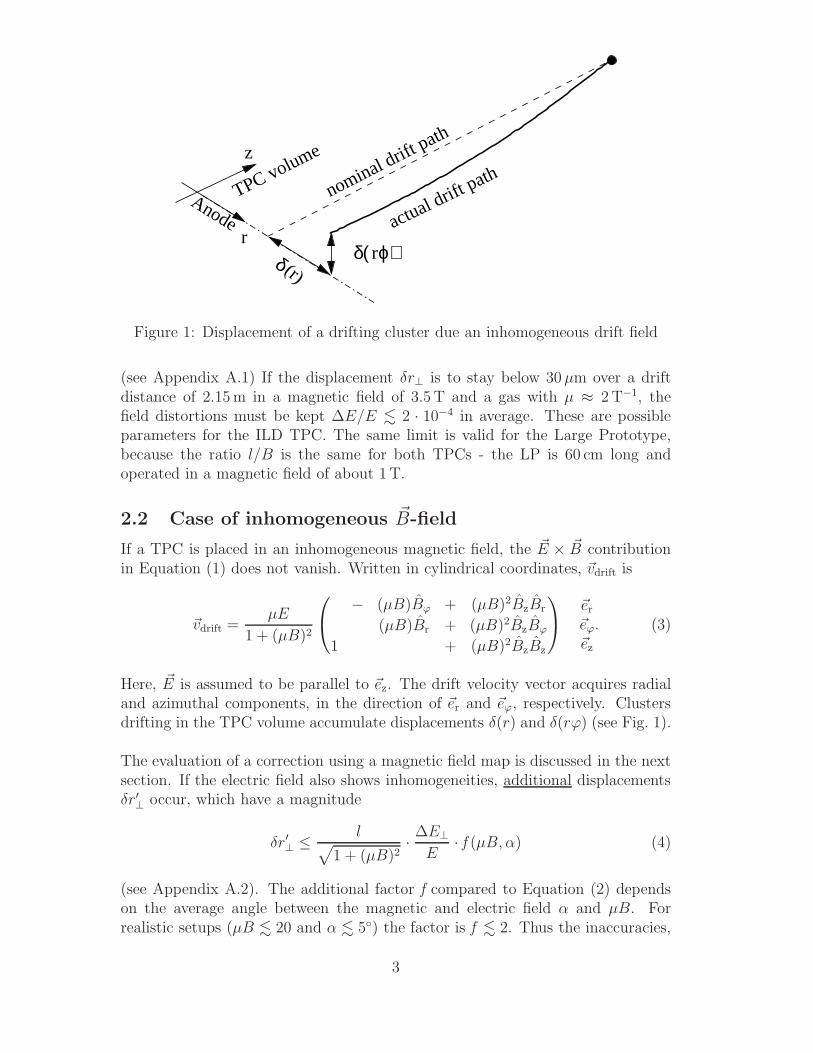
on a level of 30-µm is possible. A requirement on the measurement accuracy ofthe magnetic field of ILD is presented in [5].The next section presents briefly the mathematical framework to describe the driftof electron clusters in a TPC and the requirement for the electric field homogeneity.Section 3 discusses the correction procedures and in section 4 they are illustratedfor the case of the Large TPC Prototype (LP) [6] in the superconducting magnetPCMAG. Finally, in Sections 5 and 6, modifications to the correction procedure tocompensate for gas contaminations and a requirement on the positioning accuracyof the TPC are given.In all calculations throughout the text, the TPC is described by a cylindricalcoordinate system with ~ez along the cylinder axis. The radial vector ~er and theazimuthal vector ~eϕ lie in the anode plane. Displacements, which a cluster ac-cumulates due to field inhomogeneities while drifting in the TPC volume, aredenoted δ(r) for the radial direction and δ(rϕ) for the azimuthal direction (seeFig. 1). The correction for these displacements are Σ(r) and Σ(rϕ), respectively.

2 Drift of Low Electron Clusters in a TPC

The drift velocity ~vdrift of an electron cluster’s center of gravity in a gas volumeis described by the solution of the Langevin equation (e.g. [7])

~vdrift(/vecr) =µE

1 + (µB)2

[

E + µBE × B + (µB)2(B · E) · B]

. (1)

~E and ~B are the electric and magnetic field at the point ~r inside the TPC, respec-tively, and E and B unit vectors along ~E and ~B. The equation is typically givenwith factors ωτ , instead of µB, where τ and ω are the mean time between twoencounters of a drifting electron with gas molecules and the cyclotron frequency,respectively. These factors are equal to µB. The latter is directly accessible be-cause the electron mobility µ of the gas can be determined from simulations [8]or from a measurement of the drift velocity of electrons in the gas.

2.1 Case of homogeneous ~B-field

A TPC is typically operated with ~E and ~B aligned parallel and perpendicular tothe readout plane ( ~E and ~B parallel to ~ez). Then the term ~E × ~B in Equation (1)vanishes and ~vdrift is

~vdrift = µ~E if ~E|| ~B.

Inhomogeneities of the electric field ∆ ~E⊥ (⊥ ~ez) cause an ~E× ~B term in Equation(1) and a component of ~vdrift in a direction perpendicular to ~ez. A particle whichdrifts over a distance l in a region with the non vanishing ∆E⊥ gets displaced byδr⊥. The magnitude can be estimated by

δr⊥ =√

δ(r)2 + δ(rϕ)2 .l

√

1 + (µB)2·∆E⊥

E. (2)

2

rδ( ϕ) δ(r)

z

r

nominal drift path

Anode

TPC volume

actual drift path

Figure 1: Displacement of a drifting cluster due an inhomogeneous drift field

(see Appendix A.1) If the displacement δr⊥ is to stay below 30 µm over a driftdistance of 2.15 m in a magnetic field of 3.5 T and a gas with µ ≈ 2 T−1, thefield distortions must be kept ∆E/E . 2 · 10−4 in average. These are possibleparameters for the ILD TPC. The same limit is valid for the Large Prototype,because the ratio l/B is the same for both TPCs - the LP is 60 cm long andoperated in a magnetic field of about 1 T.

2.2 Case of inhomogeneous ~B-field

If a TPC is placed in an inhomogeneous magnetic field, the ~E × ~B contributionin Equation (1) does not vanish. Written in cylindrical coordinates, ~vdrift is

~vdrift =µE

1 + (µB)2

− (µB)Bϕ + (µB)2BzBr

(µB)Br + (µB)2BzBϕ

1 + (µB)2BzBz

~er

~eϕ

~ez

. (3)

Here, ~E is assumed to be parallel to ~ez. The drift velocity vector acquires radialand azimuthal components, in the direction of ~er and ~eϕ, respectively. Clustersdrifting in the TPC volume accumulate displacements δ(r) and δ(rϕ) (see Fig. 1).

The evaluation of a correction using a magnetic field map is discussed in the nextsection. If the electric field also shows inhomogeneities, additional displacementsδr′

⊥occur, which have a magnitude

δr′⊥≤

l√

1 + (µB)2·∆E⊥

E· f (µB, α) (4)

(see Appendix A.2). The additional factor f compared to Equation (2) dependson the average angle between the magnetic and electric field α and µB. Forrealistic setups (µB . 20 and α . 5◦) the factor is f . 2. Thus the inaccuracies,

3

caused by inhomogeneities of the electric field, stay below 30 µm if the condition∆E/E . 10−4 is fulfilled. In this case, a correction vector field with an accuracyin the 30-µm regime can be calculated analytically under the assumption of ahomogeneous electric field.

3 Correction Procedure

A correction for displacements δ(r) and δ(rϕ) caused by inhomogeneities of thedrift fields can be facilitated with a correction vector map: To reconstruct theorigin ~rorigin of a cluster, first a space point in the TPC, ~rreco., is reconstructedfrom the measurements of the TPC. This is done irrespective of any field inho-mogeneities. Then, a correction vector Σ(~rreco.) is evaluated at the position ~rreco.

and added. The correction vector points from the reconstructed position ~rreco. tothe correct origin of the cluster ~rorigin:

~rorigin = ~rreco. + ~Σ(~rreco.).

The correction ~Σ cancels δ(r) and δ(rϕ). Inaccuracies can remain after the cor-rection was applied and are given by

∆ =√

(δ(r) + Σ(r))2 + (δ(rϕ) + Σ(rϕ))2. (5)

Two ways to calculate the correction vectors ~Σ(~r) are discussed in the following.For this, it is assumed that the magnetic field is known from a measurement andthe electric field fulfills the homogeneity requirement of ∆E/E . 10−4. Therefore

the electric field is treated as homogeneous ~E = E ~ez in the drift volume.

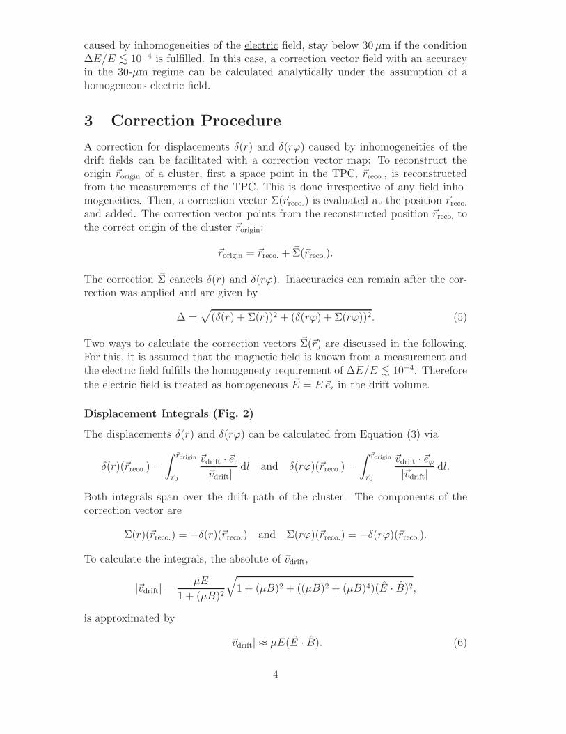
Displacement Integrals (Fig. 2)

The displacements δ(r) and δ(rϕ) can be calculated from Equation (3) via

δ(r)(~rreco.) =

∫ ~rorigin

~r0

~vdrift · ~er

|~vdrift|dl and δ(rϕ)(~rreco.) =

∫ ~rorigin

~r0

~vdrift · ~eϕ

|~vdrift|dl.

Both integrals span over the drift path of the cluster. The components of thecorrection vector are

Σ(r)(~rreco.) = −δ(r)(~rreco.) and Σ(rϕ)(~rreco.) = −δ(rϕ)(~rreco.).

To calculate the integrals, the absolute of ~vdrift,

|~vdrift| =µE

1 + (µB)2

√

1 + (µB)2 + ((µB)2 + (µB)4)(E · B)2,

is approximated by

|~vdrift| ≈ µE(E · B). (6)

4

z

r

1z=z

r recororigin

z=z

Σ

0

drift path

integration along

r0

Figure 2: Calculation of a correction vector by the integration method

This assumes small angles between B and E (�( ~E, ~B) . 30 ◦) which is the case inrealistic setups. As a second approximation, the integration along the drift pathis replaced by an integration parallel to the z axis (see Fig. 2). This is accurate,if Br and Bϕ do not show large variations between the actual drift path and theapproximated one.Hence, ~Σ(~rreco.) for a cluster which has been detected at a position ~r0 on the anodeis calculated by evaluating the integrals

Σ(r)(~rreco.) ≈ −

∫ zreco.

z0

1

1 + (µB)2

1

Bz

(

−µB Bϕ + (µB)2 BzBr

)

dz (7)

Σ(rϕ)(~rreco.) ≈ −

∫ zreco.

z0

1

1 + (µB)2

1

Bz

(

µB Br + (µB)2 BzBϕ

)

dz (8)

from z0 = 0 to zreco. = ~rreco. · ~ez. Here B · E = Bz was used.

Inverse drift (Fig. 3)

Alternatively, Σ(r) and Σ(rϕ) can be calculated by an inverse drift procedure:Starting from ~r0 on the anode, where a cluster was registered, the drift path inthe TPC volume is reconstructed. This is done with an inverse tracking procedure(Fig. 3). Iteratively, points ~ri on the drift path of the cluster are calculated by

~ri = ~ri-1 +~vdrift( ~E, ~B(~ri-1))

|~vdrift( ~E, ~B(~ri-1))|· δl and ti = ti - 1 +

δl

|~vdrift( ~E, ~B(~ri-1))|, (9)

with δl being the step width of the iterative procedure. In parallel, the drift timeti is summed up. Before a step (i → i+1) is performed, the direction of ~vdrift at

the position ~ri-1 is calculated from the electric field ~E and the local magnetic field~B(~ri-1).

5

z

r

r recororigin

0

r

1z=z

0

inverse drift

z=z

Σ

Figure 3: Calculation of a correction vector by the reverse drift

After a step has been performed, the correction vector ~Σ(~rreco.) is calculated by

~Σ(~rreco.) = ~Σ (~r0 + ti · µE ~ez) = [~ri − (~r0 + ti · µE︸︷︷︸

vdrift

~ez)].

The term ~r0 + ti · µE ~ez is equal to ~rreco. – the origin of the cluster, which will bereconstructed when the field inhomogeneities are not considered. The correctedorigin of the cluster ~rorigin is

~rorigin = ~r0 + t · µE ~ez︸ ︷︷ ︸

reconstructed position ~rreco.

+ ~Σ (~r0 + t · µE ~ez)︸ ︷︷ ︸

correction vector

(t : drift time).

The reconstruction of the drift path of clusters is able to give accurate results forany possible configuration of the magnetic field inside the TPC volume. This holdseven in the presence of significant field gradients, if the step width δl is chosensmall enough that neither Br nor Bϕ show large variations over δl. Electric fieldinhomogeneities can be considered in Equation (9) by respecting the dependency

of ~vdrift on ~E. For this a position dependent description of the electric field ~E(~r)is needed.

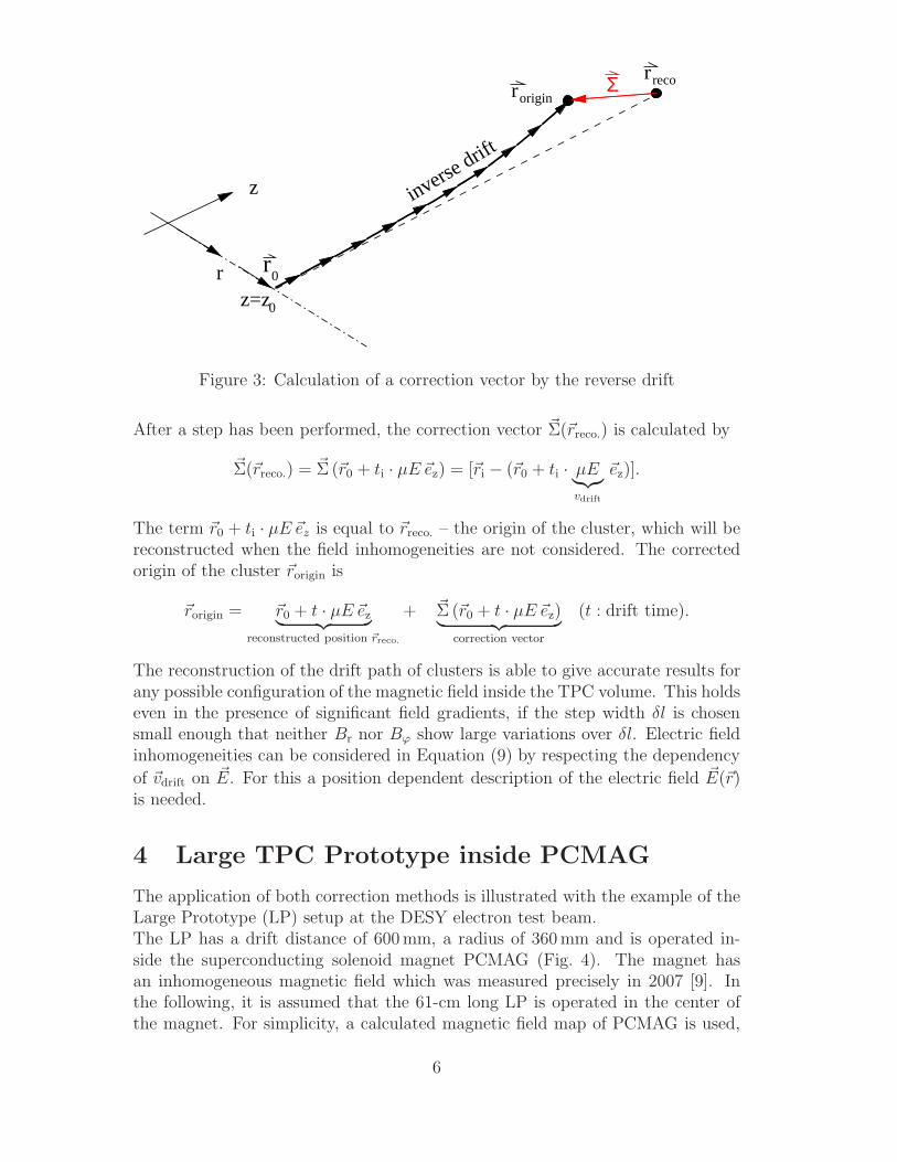
4 Large TPC Prototype inside PCMAG

The application of both correction methods is illustrated with the example of theLarge Prototype (LP) setup at the DESY electron test beam.The LP has a drift distance of 600 mm, a radius of 360 mm and is operated in-side the superconducting solenoid magnet PCMAG (Fig. 4). The magnet hasan inhomogeneous magnetic field which was measured precisely in 2007 [9]. Inthe following, it is assumed that the 61-cm long LP is operated in the center ofthe magnet. For simplicity, a calculated magnetic field map of PCMAG is used,

6

LP

TPC

PCMAG

B [T]

0

1.5

(a) magnetic field strength distribution ofPCMAG

(b) Br/B of the magnetic field inside the LPfor the central position in PCMAG

Figure 4: Magnetic field of PCMAG inside the LP

which is assumed to be rotational symmetric with a vanishing azimuthal compo-nent (Bϕ ≡ 0). Due to the symmetry, the calculation of the correction vectorscould be restricted to a two dimensional plane cut through the center of the LP.In this plane, the magnetic field map was sampled in bins of 200 µm × 200 µm.For the electron drift mobility, µ = 2 T−1 was used, which is the value of TDR gas.As a cross check, all calculations were also performed with a value of µP5 = 4 T−1

for P5 gas. The results do vary only slightly and are not significantly different.

4.1 Calculation of the Systematic Displacements

In the first step, the displacements δ(r) and δ(rϕ) for the magnetic field of PC-MAG were calculated similar to the evaluation of the correction vector field dis-cussed above (Sec. 3 and Fig 3): Starting from a cell of a 200 µm×200 µm grid ofthe LP volume, the drift path of an electron cluster was extrapolated iterativelyup to the anode. The accumulated δ(r) and δ(rϕ) were then evaluated from theend point of a cluster on the anode and the cluster’s origin. This was done suc-cessively with every cell on the grid to cover the complete volume of the LP. Theelectric field was assumed to be homogeneous ~E = E ~ez for this calculation. Hencealso µ was set constant.The results are shown in Figure 5. Displacements along z are negligibly small –typically some 10 µm – and therefore omitted.

7

(a) systematic displacement δ(r) (b) systematic displacement δ(rϕ)

Figure 5: Calculated systematic displacements δ(r) and δ(rϕ) for the LP at thecenter position inside PCMAG (see Fig. 4).

4.2 Application of the Correction

Calculation of Displacement Integrals for PCMAG

For the case of a vanishing azimuthal component of the magnetic field (Bϕ ≡ 0)the calculation of the corrections using Equations (7) and (8) simplifies to

Σ(r)(z) ≈ −

∫ z1

z0

(µB)2

1 + (µB)2

Br

Bdz′ ≈ −

z1∑

z0

(µB)2

1 + (µB)2

Br

B∆z

Σ(rϕ)(z) ≈ −

∫ z

z0

µB

1 + (µB)2

Br

Bzdz′ ≈ −

z1∑

z0

µB

1 + (µB)2

Br

Bz∆z.

The integrals were replaced by a summations with ∆z = 200 µm, because themagnetic field was not available as an analytic expression. In Figures 6(a) and6(b), the calculated components of the correction vector field are shown.The remaining inaccuracies ∆(~r) (see Eq. (5)), after applying the correction, havea magnitude of less than 10 µm (see Fig. 6(c)). The drift path of clusters beingcreated in the according regions pass areas in front of the anode where the radialcomponent of the magnetic field, Br, shows the largest variations in the radialdirection (see Fig. 4(b)). (The contour lines in this plot become perpendicularto the anode). In these areas, the integrals underestimate Br and Bϕ, which hasan effect for larger z. Going from the center towards the cathode, ∆ is reduced,because the magnetic field is symmetric to the center of the LP at z= 300 mm,except the sign of Br. Displacements accumulated in the front part of the LP(z < 300 mm) are compensated in the back part (z > 300 mm).

8

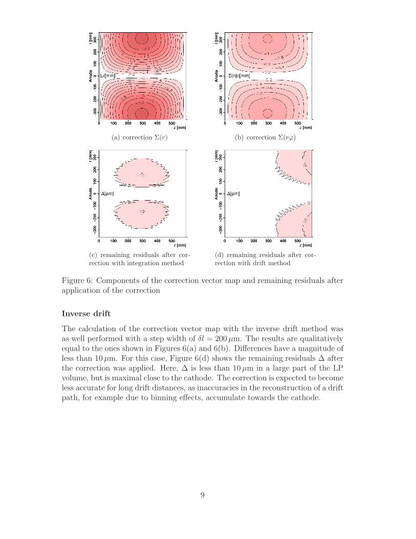
(a) correction Σ(r) (b) correction Σ(rϕ)

(c) remaining residuals after cor-rection with integration method

(d) remaining residuals after cor-rection with drift method

Figure 6: Components of the correction vector map and remaining residuals afterapplication of the correction

Inverse drift

The calculation of the correction vector map with the inverse drift method wasas well performed with a step width of δl = 200 µm. The results are qualitativelyequal to the ones shown in Figures 6(a) and 6(b). Differences have a magnitude ofless than 10 µm. For this case, Figure 6(d) shows the remaining residuals ∆ afterthe correction was applied. Here, ∆ is less than 10 µm in a large part of the LPvolume, but is maximal close to the cathode. The correction is expected to becomeless accurate for long drift distances, as inaccuracies in the reconstruction of a driftpath, for example due to binning effects, accumulate towards the cathode.

9

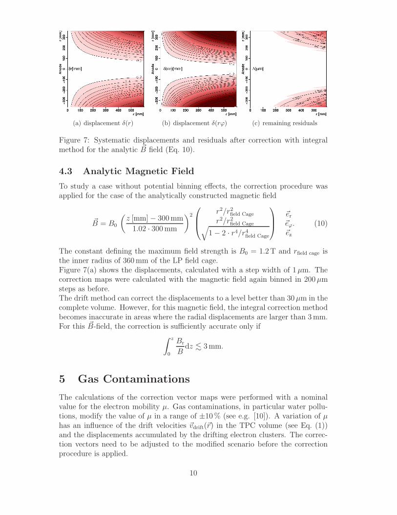
(a) displacement δ(r) (b) displacement δ(rϕ) (c) remaining residuals

Figure 7: Systematic displacements and residuals after correction with integralmethod for the analytic ~B field (Eq. 10).

4.3 Analytic Magnetic Field

To study a case without potential binning effects, the correction procedure wasapplied for the case of the analytically constructed magnetic field

~B = B0

(z [mm] − 300 mm

1.02 · 300 mm

)2

r2/r2field Cage

r2/r2field Cage√

1 − 2 · r4/r4field Cage

~er

~eϕ

~ez

. (10)

The constant defining the maximum field strength is B0 = 1.2 T and rfield cage isthe inner radius of 360 mm of the LP field cage.Figure 7(a) shows the displacements, calculated with a step width of 1 µm. Thecorrection maps were calculated with the magnetic field again binned in 200 µmsteps as before.The drift method can correct the displacements to a level better than 30 µm in thecomplete volume. However, for this magnetic field, the integral correction methodbecomes inaccurate in areas where the radial displacements are larger than 3 mm.For this ~B-field, the correction is sufficiently accurate only if

∫ z

0

Br

Bdz . 3 mm.

5 Gas Contaminations

The calculations of the correction vector maps were performed with a nominalvalue for the electron mobility µ. Gas contaminations, in particular water pollu-tions, modify the value of µ in a range of ±10 % (see e.g. [10]). A variation of µhas an influence of the drift velocities ~vdrift(~r) in the TPC volume (see Eq. (1))and the displacements accumulated by the drifting electron clusters. The correc-tion vectors need to be adjusted to the modified scenario before the correctionprocedure is applied.

10

In case of the correction method using the calculated displacement integrals(Sec. 3), the adjustment can be performed by the scaling the prefactors in Equa-tions (7) and (8) according to

(µB)2

1 + (µB)2→

µ′2

µ2

1 + (µB)2

1 + (µB′)2and

µB

1 + (µB)2→

µ′

µ

1 + (µB)2

1 + (µ′B)2. (11)

µ′ is the modified value of µ. For PCMAG, B can be assumed to be a con-stant mean value, although the magnetic field of the PCMAG shows variations instrength of ±3 %. The remaining residuals after the correction are of the order15 µm, if µ′ does not differ from µ by more than ±10 %.The scaling factors derived form the adaption procedure can also be used to adapta correction field which was evaluated with the drift method.

6 Positioning Accuracy of the TPC

To derive a condition for the positioning accuracy which is required for the LPinside the PCMAG that the correction works accurately, it is assumed that theLP is displaced in the r-direction by ∆r 6= 0 with respect to its nominal position.In this case, the correction vector for a cluster, which has been reconstructed at~rreco. is found at the modified position ~rreco. + ∆r · ~er. If ∆r is assumed to vanish,the correction is inaccurate by

∆Σ(r) =

√(

∂

∂rΣ(r)

)2

+

(∂

∂rΣ(rϕ)

)2

· ∆r

The same argument for the longitudinal component yields the inaccuracy

∆Σ(z) =

√(

∂

∂zΣ(r)

)2

+

(∂

∂zΣ(rϕ)

)2

· ∆z

For the LP/PCMAG setup, the magnitude of the largest derivatives can be esti-mated from the correction vector map in Figures 6(a) and 6(b). These are

∂

∂rΣ(r) |max ≈ 0.010 and

∂

∂rΣ(rϕ) |max ≈ 0.005

∂

∂zΣ(r) |max ≈ 0.016 and

∂

∂zΣ(rϕ) |max ≈ 0.008.

∆Σ(r) and ∆Σ(z) become

Σ(r) ≈ 0.011 ∆r and Σ(z) ≈ 0.018 ∆z.

The additional inaccuracy of the correction is limited to 10 µm, if ∆z and ∆r areboth smaller than 0.5 mm.

11

7 Next Steps

The correction methods presented in this note can be applied to the data takenwith the Large TPC Prototype (LP) infrastructure at DESY. As said before, theLP is operated inside the well-measured magnetic field of the superconductingmagnet PCMAG. Particle tracks are produced inside the volume of the LP byelectrons from the DESY test beam.By the end of 2010 it is planned to operate the LP with a large readout structureof about a quarter of square meter. In parallel, a set of silicon detectors will beprepared and installed directly on the outside of the LP. These additional detectorswill perform precise measurements of passing test beam electrons and deliverindependent reference points of the particle trajectories. In the data analysis,it will be possible to compare corrected trajectories with the external referencepoints.

References

[1] ILD Collaboration, ILD Letter of Intent, DESY 2009-87, KEK 2009-6

[2] J. Brau et al. [ILC Collaboration], arXiv:0712.1950.

[3] W. Wiedenmann, Distortion Corrections in the ALEPH TPC,http://wisconsin.cern.ch/˜wiedenma/TPC/Distortions/Cern LC.pdf, 2010

[4] A. Vogel, DESY-THESIS-2008-036, 2008

[5] R. Settles, W. Wiedenmann, LC-DET-2008-002, ILC-NOTE-2008-048, 2008

[6] for information see http://www.eudet.org and http://www.lctpc.org (2010)

[7] W. Blum, L. Rolandi, Particle Detection with Drift Chambers, Springer,ISBN 35-4056-425-X (1993)

[8] for information see the magboltz webpagehttp://ref.web.cern.ch/ref/CERN/CNL/2000/001/magboltz

[9] C. Grefe, DESY-THESIS-2008-052, 2008

[10] F. Stover, DESY-THESIS-2007-011, 2007

A Derivation of Equations (2) and (4)

A.1 Displacement due to electric field inhomogeneities in

a homogeneous magnetic field

To derive Equation (2), it is assumed that the magnetic field in the TPC is~B = B~ez. In a point of the TPC volume, the electric field shall have a field

12

Ano

de

Cat

hode

EE

B

α

r

z

∆

Figure 8: Definition of α = �( ~E, ~B)

EE∆

B

δ

r

z

rdrift ∆

v (E)drift

v (E+ E)

Figure 9: Definition of ~vdrift(∆E 6= 0)and ~vdrift(∆E = 0)

component in the radial direction, namely ~E = Ez ~ez + Er ~er. Introducing theangle α = �( ~E,~ez) (see Figure 8), this can be rewritten as

~E = E(cos α~ez + sin α~er).

In this point, the drift velocity vector is

~vdrift =µE

1 + (µB)2

[sin α~ex + (µB) sinα~ey + cos α · (1 + (µB)2)~ez

](12)

and has the absolute value

|~vdrift| =µE

1 + (µB)2

√

1 + (1 + cos2 α) · (µB)2 + (µB)4 cos2 α ≈µE cos α

√

1 + (µB)2.

(13)

Combining Equations (12) and (13), the displacement δ⊥, which the cluster sumsup while drifting a distance l in the vicinity of the point, calculates to

δr⊥ =

√(~vdrift · ~er)2 + (~vdrift · ~eϕ)2

|~vdrift|· l ≈

l√

1 + (µB)2

sin α

cos α.

With the approximation tan α ≈ sin α = ∆E/E for small α, this is

δr⊥ ≈l

√

1 + (µB)2

∆E

E.

If ∆E has its maximum in the considered point, δ⊥ for the maximum drift distanceL of the TPC can be estimated by replacing l by L in this equation.

A.2 Inaccuracy of a correction vector map due to electricfield inhomogeneities

Equation (2) is an estimation on the inaccuracy of a correction for an inhomo-geneous drift field caused by electric field inhomogeneities. It is derived under

13

the assumption that the magnetic field ~B is measured and the electric field as-sumed to be homogeneous ~E = E ~ez. In this case, the drift velocity vector~vdrift = ~vdrift(∆E = 0) is given by (3). If a small additional electric field ho-

mogeneity ∆~E = ∆E ~er is present in a point of the TPC, the local ~vdrift is

~vdrift(∆E 6= 0) ≈µE

1 + (µB)2

∆E/E − (µB)Bϕ + (µB)2(∆E/E Br + Bz) Br

(µB)(Br − ∆E/E Bz) + (µB)2(∆E/E Br + Bz) Bϕ

1 + (µB)(∆E/E Bϕ) + (µB)2(∆E/E Br + Bz) Bz.

. (14)

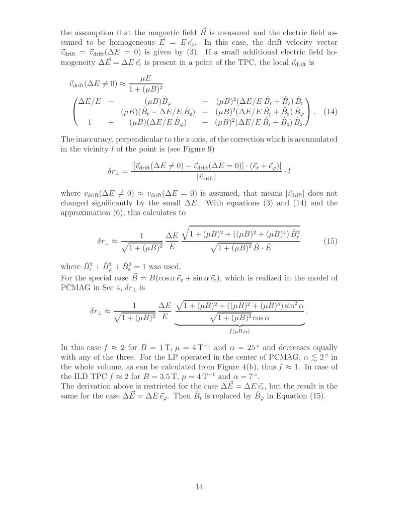
The inaccuracy, perpendicular to the z-axis, of the correction which is accumulatedin the vicinity l of the point is (see Figure 9)

δr⊥ =|[~vdrift(∆E 6= 0) − ~vdrift(∆E = 0)] · (~er + ~eϕ)|

|~vdrift|· l

where vdrift(∆E 6= 0) ≈ vdrift(∆E = 0) is assumed, that means |~vdrift| does notchanged significantly by the small ∆E. With equations (3) and (14) and theapproximation (6), this calculates to

δr⊥ ≈1

√

1 + (µB)2

∆E

E

√

1 + (µB)2 + ((µB)2 + (µB)4) B2r

√

1 + (µB)2 B · E(15)

where B2r + B2

ϕ + B2z = 1 was used.

For the special case ~B = B(cos α~ez + sin α~er), which is realized in the model ofPCMAG in Sec 4, δr⊥ is

δr⊥ ≈1

√

1 + (µB)2

∆E

E

√

1 + (µB)2 + ((µB)2 + (µB)4) sin2 α√

1 + (µB)2 cos α︸ ︷︷ ︸

f (µB,α)

.

In this case f ≈ 2 for B = 1 T, µ = 4 T−1 and α = 25 ◦ and decreases equallywith any of the three. For the LP operated in the center of PCMAG, α . 2 ◦ inthe whole volume, as can be calculated from Figure 4(b), thus f ≈ 1. In case ofthe ILD TPC f ≈ 2 for B = 3.5 T, µ = 4 T−1 and α = 7 ◦.The derivation above is restricted for the case ∆~E = ∆E ~er, but the result is thesame for the case ∆ ~E = ∆E ~eϕ. Then Br is replaced by Bϕ in Equation (15).

14