Corrections for improved quantitative accuracy in SPECT

and planar scintigraphic imaging

ANNE LARSSON

Department of Radiation Sciences, Radiation Physics Umeå University, Sweden

2005

2

Cover illustration: The logarithm of a 123I point spread function. The point source was simulated at 14.0 cm distance from the collimator in air, with the SIMIND version described in Paper V, using parameters corresponding to a GE Millennium MPR with 2.3 × 2.3 m2 field of view. The grey scale is processed.

© Anne Larsson 2005 ISBN: 91-7305-938-2 Printed by Print & Media, 2001342, Umeå, Sweden

•

3

To Björn, family and friends

If you don't care where you are,

you ain't lost.

Rune’s Rule

4

ABSTRACT

A quantitative evaluation of single photon emission computed tomography (SPECT) and planar scintigraphic imaging may be valuable for both diagnostic and therapeutic purposes. For an accurate quantification it is usually necessary to correct for attenuation and scatter and in some cases also for septal penetration. For planar imaging a background correction for the contribution from over- and underlying tissues is needed. In this work a few correction methods have been evaluated and further developed. Much of the work relies on the Monte Carlo method as a tool for evaluation and optimisation. A method for quantifying the activity of 125I-labelled antibodies in a tumour inoculated in the flank of a mouse, based on planar scintigraphic imaging with a pin-hole collimator, has been developed and two different methods for background subtraction have been compared. The activity estimates of the tumours were compared with measurements in vitro. The major part of this work is attributed to SPECT. A method for attenuation and scatter correction of brain SPECT based on computed tomography (CT) images of the same patient has been developed, using an attenuation map calculated from the CT image volume. The attenuation map is utilised not only for attenuation correction, but also for scatter correction with transmission dependent convolution subtraction (TDCS). A registration method based on fiducial markers, placed on three chosen points during the SPECT examination, was evaluated. The scatter correction method, TDCS, was then optimised for regional cerebral blood flow (rCBF) SPECT with 99mTc, and was also compared with a related method, convolution scatter subtraction (CSS). TDCS has been claimed to be an iterative technique. This requires however some modifications of the method, which have been demonstrated and evaluated for a simulation with a point source. When the Monte Carlo method is used for evaluation of corrections for septal penetration, it is important that interactions in the collimator are taken into account. A new version of the Monte Carlo program SIMIND with this capability has been evaluated by comparing measured and simulated images and energy spectra. This code was later used for the evaluation of a few different methods for correction of scatter and septal penetration of 123I brain SPECT. The methods were CSS, TDCS and a method where the corrections for scatter and septal penetration are included in the iterative reconstruction. This study shows that quantitative accuracy in 123I brain SPECT benefits from separate modelling of scatter and septal penetration.

•

5

LIST OF PAPERS

This thesis is based on the following papers which are referred to by their Roman numerals in the text. I. Anne Larsson, Lennart Johansson, Rauni Rossi Norrlund, Katrine Riklund

Åhlström. Methods for estimating uptake and absorbed dose in tumours from 125I labelled monoclonal antibodies, based on scintigraphic imaging of mice. Acta Oncologica 1999 38 361-365

II. Anne Larsson, Lennart Johansson, Torbjörn Sundström, Katrine Riklund

Åhlström. A method for attenuation and scatter correction of brain SPECT based on CT-images. Nucl Med Commun 2003 24 411-420

III. Anne Larsson, Lennart Johansson. Transmission dependent convolution

subtraction of 99mTc-HMPAO rCBF SPECT – A Monte Carlo study. IEEE

Trans Nucl Sci 2005 52 231-237 IV. Anne Larsson, Lennart Johansson. Scatter-to-primary based scatter fractions

for transmission dependent convolution subtraction of SPECT images. Phys

Med Biol 2003 48 N323-N328 V. Michael Ljungberg, Anne Larsson, Lennart Johansson. A new collimator

simulation in SIMIND based on the Delta-Scattering technique. Accepted for publication IEEE Trans Nucl Sci

VI. Anne Larsson, Michael Ljungberg, Susanna Jakobson Mo, Katrine Riklund,

Lennart Johansson. Correction for scatter and septal penetration in 123I brain SPECT imaging – A Monte Carlo study. Submitted

Paper I-V have been reproduced with permission from the publishers.

6

TABLE OF CONTENTS 1 INTRODUCTION 9 2 SCINTIGRAPHIC IMAGING 11

2.1 The gamma camera 11 2.1.1 Gamma cameras used in this work 12

2.2 Single photon emission computed tomography (SPECT) 15 2.2.1 Reconstruction of SPECT images 15

2.3 Radiopharmaceuticals 17

2.4 Photon interactions with matter 19 2.4.1 Attenuation 20

2.5 Scintigraphic studies in this work 21 3 QUALITY OF SCINTIGRAPHIC IMAGES 22

3.1 Contrast 22

3.2 Noise 22

3.3 Quality parameters of a gamma camera 24 3.3.1 Spatial resolution 24

3.3.2 Sensitivity 25

3.3.3 Uniformity 26

3.3.4 Energy resolution 27

3.3.5 Count rate performance 27

4 QUANTITATIVE IMAGING 28

4.1 Absolute quantification 28 4.1.1 Absolute quantification in this work 29

4.2 Relative quantification 30 4.2.1 Relative quantification in this work 30

5 THE MONTE CARLO METHOD 32

5.1 Monte Carlo simulations in this work 33 5.1.1 Monte Carlo simulations of collimator interactions 33

6 CORRECTIONS FOR QUANTITATIVE SPECT 35

6.1 Attenuation correction 35 6.1.1 Transmission measurements with a radionuclide 37

6.1.2 Transmission measurements with a CT scanner 39

6.1.3 Attenuation correction in this work 40

6.2 Scatter correction 42 6.2.1 Energy window techniques 44

6.2.2 Convolution techniques 46

6.2.3 Scatter correction in an iterative reconstruction procedure 47

6.2.4 Scatter correction in this work 48

6.3 Compensation for collimator-detector response (CDR) 51 6.3.1 CDR compensation in this work 54

•

7

6.4 Correction for septal penetration 56 6.4.1 Energy window techniques 58

6.4.2 Convolution techniques 59

6.4.3 Septal penetration in an iterative reconstruction procedure 59

6.4.4 Correction for septal penetration in this work 60

7 CORRECTIONS FOR PLANAR SCINTIGRAPHIC IMAGING 62

7.1 Attenuation correction 62

7.2 Background correction 65

7.3 Attenuation and background correction in this work 66 8 SUMMARY AND CONCLUSIONS 69

8.1 Paper I 69

8.2 Paper II 69

8.3 Paper III 69

8.4 Paper IV 70

8.5 Paper V 70

8.6 Paper VI 71

9 FUTURE PERSPECTIVES 72

10 ACKNOWLEDGEMENTS 73

11 REFERENCES 75

8

ABBREVIATIONS 123I-IMP N-isopropyl-p-123I-amphetamine 1D One-dimensional 2D Two-dimensional 3D Three-dimensional CDR Collimator-detector response cpm Counts per minute cps Counts per second CSS Convolution scatter subtraction CT Computed tomography DAT Dopamine transporter ESSE Effective source scatter estimation FBP Filtered backprojection FWHM Full width at half maximum FWTM Full width at tenth maximum GP General purpose HEGP High energy general purpose HMPAO Hexamethyl propyleneamine oxime HR High resolution LE Low energy LEGP Low energy general purpose ME Medium energy MEGP Medium energy general purpose MIBG Meta-iodobenzylguanidine MIRD Medical Internal Radiation Dose MLEM Maximum likelihood expectation maximisation MRT Magnetic resonance tomography NEMA National Electrical Manufacturers Association NMSE Normalised mean square error OSEM Ordered subsets expectation maximisation PET Positron emission tomography PM Photomultiplier rCBF Regional cerebral blood flow RIT Radioimmunotherapy ROI Region of interest SDSE Slab-derived scatter estimation SLSF Scatter line spread function SPECT Single photon emission computed tomography TDCS Transmission dependent convolution subtraction TEW Triple energy window VOI Volume of interest

•

9

1 INTRODUCTION In single photon emission computed tomography (SPECT) and planar scintigraphic imaging, the distribution of a radiopharmaceutical in vivo is studied. In absence of some physical degrading factors, the SPECT images would reflect the 3D distribution of the radiopharmaceutical, while the planar images would reflect the corresponding 2D projections through the imaged object. In reality the images are seriously affected by attenuation, scatter and detector response, and for some radionuclides also septal penetration. It is however possible to correct for these effects, more or less accurately. For a visual interpretation, planar images are seldom corrected. The effect of attenuation in such cases can even be an advantage since it can provide depth information of the radiopharmaceutical distribution, if images from opposing views are acquired. If SPECT images are corrected for the purpose of visual interpretation it is in most cases only for attenuation. A visual interpretation should however benefit from corrections also for scatter and detector response in many cases since the resulting increase in image quality can simplify lesion detection. Corrections are more important and widely applied for quantitative evaluations of the images, especially for absolute quantification where the activity is calculated. To know the activity in a specific organ or a tumour is essential for calculating the absorbed dose to that part of the body, which for example can be of interest for dose planning in radionuclide therapy. Absolute quantification from planar images requires usually also a background correction for the contribution of registrations from activity in over- and underlying tissues. For a relative quantification, the calibration to activity is not necessary, but the images should preferably reflect the distribution of the radiopharmaceutical, which requires corrections. In this case the counts in different regions in the images can be compared and this is often of interest for diagnostic purposes. The aims of this work were to evaluate and further develop corrections that improve the quantitative accuracy of SPECT (in particular) and planar scintigraphic imaging. Most of the work concerns brain imaging, since most of the SPECT research at Norrlands University Hospital, Umeå University has been concentrated on regional cerebral blood flow (rCBF) or the dopamine transporter and receptor system in the brain. In many cases, however, the methods are also applicable to other parts of the body. This work is focused on corrections for background activity, attenuation, scatter, septal penetration and detector response. The Monte Carlo method is used as a tool for evaluation and optimisation in many parts of the work. More specific the aims of the present work were to:

• Develop and evaluate a quantitative method for determining the uptake of 125I-labelled compounds in a tumour inoculated in the flank of a mouse, based on planar scintigraphic imaging with a pin-hole collimator. The evaluation includes the comparison of two different methods to correct for the background

10

activity. This work on planar scintigraphic imaging can be seen as an introduction to the more complex world of SPECT. The method is described in Paper I.

• Develop and evaluate a method for attenuation and scatter correction of brain

SPECT based on computed tomography (CT) images of the same patient, where the registration of the CT and SPECT image volumes should be performed using fiducial markers that only need to be present during the SPECT examination. The method is evaluated for 99mTc Hexamethyl propyleneamine oxime (HMPAO) rCBF SPECT and is described in Paper II.

• Further developing of the scatter correction method used in the previous study,

transmission dependent convolution subtraction (TDCS), by determining the optimal geometry for deriving scatter fractions as a function of attenuation path length, and the optimal scatter kernel, for 99mTc HMPAO rCBF SPECT. TDCS is also compared with convolution scatter subtraction (CSS) and this is described in Paper III. The aim was also to introduce a few adjustments in the correction method to make it suitable for many iterations, which is described in Paper IV.

• To contribute to the evaluation of a new version of the Monte Carlo program

SIMIND that can take interactions in the collimator into account. This is important when the effect of septal penetration is studied using Monte Carlo simulations. This is described in Paper V.

• To use this Monte Carlo program to evaluate a few correction methods for

scatter and septal penetration; CSS, two TDCS versions and one method included in the iterative reconstruction which uses the effective source scatter estimation (ESSE) to model scatter and collimator-detector response (CDR) including septal penetration. The aim was also to implement a distance-independent compensation for CDR for geometrically mean valued projection images. This study is described in Paper VI.

•

11

2 SCINTIGRAPHIC IMAGING In scintigraphic imaging, the distribution of an administered gamma photon emitting radiopharmaceutical in vivo is visualised using external detectors. 2D images can be acquired using a stationary gamma camera and 3D images can be acquired using SPECT or positron emission tomography (PET). SPECT is a common technique available at most hospitals while PET requires special equipment and preferably locally produced radionuclides and is not an issue of this work. In scintigraphic imaging, “functional images” are produced, where the distribution of the radiopharmaceutical is visualised. Functional imaging is important for diagnostics of different diseases since changes of function can occur long before any consequential changes in morphology. Many biochemical processes can be studied using scintigraphic imaging and it is therefore an important tool, both for diagnostics and research. 2.1 The gamma camera The detector used for scintigraphic imaging is called a gamma camera or Anger camera. It was developed in the late 1950’s by Hal Anger (Anger 1958) and has for a long time been a standard imaging device in nuclear medicine. The basic components of the gamma camera today are in many cases the same as when it was invented, but its performance has been improved over the years, especially by the introduction of digital electronic components and multiple head systems. A schematic figure of the gamma camera detector can be seen in Fig. 1. The detector is attached to a gantry for motion control.

Fig. 1. The gamma camera.

The collimator, which can be of different types, is closest to the imaged object and sets the acceptance angle for detection of the emitted gamma photons. The parallel-hole collimator is the most popular one and it consists of a lead plate with closely packed parallel holes, usually with hexagonal form. The lead “walls” between the holes are called septa. The hole diameter, collimator thickness and septal thickness depend on the resolution/sensitivity and the photon energy range for which the collimator is optimised. In most cases the hole diameter is a few millimetres, while the collimator thickness is a few centimetres. Parallel-hole collimators were used in the studies described in Paper II-

Collimator NaI(Tl)-crystal

Light guide

PM-tubes

Electronics for position and energy

12

VI. In the study described in Paper I, a pin-hole collimator was used. It is formed as a lead cone with a small hole at the apex, facing the imaged object. With the pin-hole collimator the size of the image will depend on the distance from the object to the pin-hole, which is not the case for parallel-hole collimators. The pin-hole collimator is convenient when the imaged objects are small, for example small animals or small organs like the thyroid, since these objects can be magnified on the image. There are also other types of collimators, for example fan-beam, cone-beam and slant-hole collimators (Ricard 2004). The detector material in the gamma camera is generally a NaI(Tl)-crystal. It is coated with a thin Al-layer at the front side and the edges to protect from outside light and moisture. The crystal is typically about 1 cm thick, which gives a high detection probability for photons with energies up to a few hundred keV. When a gamma photon interacts in the crystal, light photons are created, and the number of light photons is proportional to the energy deposited in the crystal. The rear side of the crystal is optically coupled to a light guide of glass, which protects the crystal and leads the light photons to an array of photomultiplier tubes, which are optically coupled to the light guide. The PM-tubes convert the light photons to electrons on a photocathode and amplify the number of electrons in a dynode-chain. This results in a measurable electrical pulse at the anode of those PM-tubes that are hit by the light photons. These pulses are processed through a matrix of electronic circuits to give signals with amplitudes proportional to the location of the gamma photon interaction, and the energy deposited in the crystal. Logical and discrimination processes are then taking place to sort out the interactions in the crystal that should contribute to the image. 2.1.1 Gamma cameras used in this work

Four different gamma cameras have been used for measurements or simulations in this work, and they are all located at the Nuclear Medicine department at Norrlands University Hospital in Umeå. The manufacturer of these cameras is General Electric (WI, USA). The Porta Camera is an old analogue camera used for thyroid imaging and it can be seen in Fig. 2 a. In the study described in Paper I, it was equipped with a pin-hole collimator for imaging of mice. The Neurocam, shown in Fig. 2 b, is a dedicated brain camera with three detectors with a fixed radius of rotation of 12.25 cm. This camera is used in the studies described in Paper II-IV. The Millennium MPR is a multi-purpose rectangular single headed gamma camera, and it can be seen in Fig. 2 c. It was chosen for Paper V because of its wide scatter free surroundings, which makes it suitable for comparison of Monte Carlo simulations and measurements. The Millennium MG, shown in Fig. 2 d, is a multi-purpose dual-headed gamma camera. The detectors and collimators of this camera are the same as for the Millennium MPR. It was chosen for the simulations described in Paper VI for brain SPECT since it was clear that the Neurocam soon would be replaced. During that study the new camera was however not yet decided, and the Millennium MG is the second choice brain camera at the Nuclear Medicine department in Umeå.

•

13

Fig. 2 a. Porta Camera

Fig. 2 b. Neurocam

14

Fig. 2 c. Millennium MPR

Fig. 2 d. Millennium MG

•

15

2.2 Single photon emission computed tomography (SPECT) SPECT is a method where 2D projections are acquired with a gamma camera at different angles around the patient. The projections are used for reconstruction of a 3D image volume, which ideally should correspond to the activity distribution in the patient. A continuous acquisition of data is possible but requires complicated data management (Hamilton 2004), and in most cases a “step and shoot” technique is used instead, with no data collected during the detector movements. The 2D projections are acquired in a circular or elliptical orbit around the patient, and the number of projections usually varies between 64 and 128, equally distributed in space. A complete acquisition measures projections over a 360º rotation but a restricted acquisition of 180º is sometimes used. A multiple head system is advantageous for SPECT since it is a relatively time-consuming procedure. 2.2.1 Reconstruction of SPECT images

The classical method of image reconstruction is the filtered backprojection (FBP) technique (Cormack 1963, Hounsfield 1973), which is based on the inverse of the Radon transform (Radon 1917). In this method the projection data (each row of pixels in the acquired planar images) is filtered in the frequency plane with a ramp filter. The filtered projections are then transformed to the spatial plane and backprojected from the acquired angles, to give transaxial images. The ramp filter is proportional to frequency, with 0 at 0 frequency, and is used to remove blurring introduced by the backprojection step. Since it is a high-pass filter that amplifies high frequency noise, the projection images are usually filtered with a low-pass filter before reconstruction. A review of filtering in SPECT has been published for example by Van Laere et al (2001). FBP is fast and simple to implement but can give streak artifacts, due to the limited number of projections. The calculated transaxial images build a 3D image volume that can be sliced in any direction. Iterative techniques have long been known to possess some advantages compared with the filtered back projection technique. They have however only recently come into clinical use because of the computer capacity required. Iterative techniques are based on the following equation (Vandenberghe et al 2001):

∑=b

bdbpdn )(),()(* λ (1)

where λ(b) is the digitised true tracer distribution as a 1D vector, p(b,d) is a probability matrix describing the probability of detecting a photon originating in voxel b in detection bin d and n*

(d) is the 1D vector of acquired projection data. This forms a large set of linear equations that theoretically can be solved for λ(b). The direct inversion is however rather slow, and numerical instabilities can occur, and the equation is therefore usually solved iteratively (Vandenberghe et al 2001). The iterations start with an initial estimate λ0(b) which for example can be a blank image, a homogeneous phantom image, or a reconstruction using FBP. The estimate should then be improved at every iteration step by comparing the calculated projections with the acquired ones, and different

16

iterative techniques handle this in different ways. Examples of iterative algorithms that use algebraic methods can be seen in the following references: Gordon et al (1970), Gilbert (1972) and Goitein (1972), and examples of different statistical methods can be seen in: Herbert and Leahy (1989), Gindi et al (1993), Hudson et al (1994) and Byrne (1996). A well-known statistical iterative technique is the maximum likelihood expectation maximisation (MLEM) method (Shepp and Vardi 1982, Lange and Carson 1984). It iteratively maximises a likelihood function and takes the Poisson nature of the data into account. It obtains a new estimate of λ(b) for iteration step k+1 according to the following equation:

∑∑∑

=+ d

b kd

kk

bdbp

dndbp

dbp

bb

'

*

1)'(),'(

)(),(

),(

)()(

λ

λλ (2)

The sum in the denominator within the brackets can be called the projection step. This is the calculation of new estimated projection data (see Eq. 1) from the current estimation of the activity distribution. The sum over the brackets is called the back-projection step, where the calculated projections are compared with the measured projections to generate a new iterand that should be closer to the most likely solution where the likelihood is maximised (Shepp and Vardi 1982). For 3D reconstructions, the probability matrix is very large (the total number of voxels in the images to be reconstructed times the total number of pixels in all projections). Therefore it is usually not calculated and stored, and the needed matrix elements are instead calculated “on the fly” (King et al 2004). The MLEM method is relatively slow, and is seldom used as it is. Hudson and Larkin (1994) have suggested a way to group the data into smaller subsets to decrease computing time. This method is called ordered subsets expectation maximisation (OSEM) and today it is widely used and often included in modern clinical software. The subsets are comprised of evenly spread projections around the patient, and two projections have been suggested as the minimum number per subset (Hudson and Larkin 1994). In theory, it is however better to use at least four projections per subset since the sum of counts in the projections forming each subset ideally should be equal for all subsets, and this requirement is more likely to be fulfilled if the subset size is not too small (Hutton and Lau 1997). The decrease in computing time in comparison with the MLEM technique is roughly a factor of the number of subsets used, and if we have 64 projections and four projections/subset, the computing time decreases with a factor of 16. When using OSEM, one iteration is defined as a pass through all the subsets. OSEM has been used for all reconstructions in this work, with four projections per subset.

•

17

MLEM converges to the maximum likelihood solution (Shepp and Vardi 1982) but it appears that the limit image of the OSEM reconstruction depends on the last projection processed (Hudson and Larkin 1994). It has therefore been of interest to develop accelerated techniques that do converge to the maximum likelihood solution (Browne and De Pierro 1996, Hsiao et al 2004). The importance of a converging method can however be questioned since the number of iterations usually is well below the limit of convergence when using maximum likelihood-based techniques. OSEM has also been shown to give images that are very similar to images using MLEM, using the corresponding number of iterations (Hutton et al 1997). An advantage of iterative methods like MLEM and OSEM is that models for attenuation, scatter, collimator-detector response (CDR), septal penetration and other effects like patient motion and tracer kinetics can be incorporated into the reconstruction (Hutton et al 1997). Compensation for attenuation, scatter, CDR and septal penetration will be discussed further in later sections. 2.3 Radiopharmaceuticals

In scintigraphic imaging, the distribution of a radiopharmaceutical is visualised. A radiopharmaceutical consists of two principal components, the photon emitting radionuclide and the pharmaceutical compound. The radionuclide is needed for detection while the pharmaceutical dictates the distribution within the body. Some ready-to-use radiopharmaceuticals can be delivered by the manufacturers, but in most cases the radionuclide compound is labelled to the pharmaceutical at the hospital. In rare cases the radionuclide is labelled to material from the patient’s body, for example white blood cells (Johansson and Johansson 1998). When choosing a radionuclide for diagnostic imaging, a number of factors must be accounted for (Johansson and Johansson 1998). For radiation protection reasons, it is important that the dose delivered to the patient is as low as reasonably achievable. Alfa and beta radiation, and emission of photons with energies other than the principal energy used for imaging, should therefore preferably be avoided. The preferred energy range of the gamma photons used for imaging is roughly between 70 and 200 keV. For lower gamma energies, too many photons will be attenuated in the patient and contribute to the dose but not to the images, and higher energies require medium- or high-energy collimators which have a negative effect on spatial resolution and sensitivity. The half-life of the radioactive decay is of course important. Enough activity must be left in the patient at the time of imaging, but after the examination the remaining activity serves no useful purpose and gives the patient unnecessary dose. Stable chemical bounding between the radionuclide and the pharmaceutical is important since the examination becomes useless if the two have been separated at the time of imaging. It is also advantageous if the labelling procedure is uncomplicated and if the radionuclide is inexpensive. Examples of radionuclides used for diagnostic imaging are 99mTc, 133Xe, 111In, 123I, 201Tl, 131I and 67Ga (Jönsson and Richter 2004).

18

When choosing a radionuclide for radionuclide therapy, the characteristics above concerning dose are reversed to some degree. In this case the half-life, type of radiation and particle energies should be matched to give a high dose to the treated tissues. Photon emissions are needed if imaging is used to follow up the treatment. Examples of radionuclides used for therapy are 131I, 90Y, 153Sm, 32P and 89Sr (Jönsson and Richter 2004). Some characteristics of the radionuclides used in this work are presented in Table I (ICRP 1983). In the study described in Paper I, we used a radionuclide that is rarely used for imaging of humans, 125I. The energies of the gamma and characteristic X-ray photons emitted from the decay of 125I are too low to be optimal for patient examinations, but since the “patients” in that study were mice, enough photons could escape and contribute to the images. 125I has a relatively long half-life, which makes it suitable for long time studies. The next radionuclide in Table I, 99mTc, is the dominant radionuclide in diagnostic imaging, and in 2004 it was used for 94 % of the imaging examinations at the Nuclear Medicine department in Umeå. It possesses all the positive characteristics described above except for simple labelling procedures, and therefore it can still not be used for all types of examinations that otherwise would be suitable for 99mTc. It is relatively inexpensive since it can be generated daily from a “Tc-generator” containing 99Mo, which has a half-life of 66 h. 99mTc was used for simulations and measurements in the studies described in Paper II-IV. In the studies described in Paper V and VI, we used the radionuclide 123I. In 2004 it was used for 33 % of the brain examinations at the Nuclear Medicine department in Umeå, but only 4 % of the total number of imaging examinations. Since 123I is a halogen the labelling procedure is relatively uncomplicated, but the emission of electrons gives the patient a higher dose compared with 99mTc-labelled compounds. 123I also emits high energy gamma photons that degrade image quality, and the most dominant high energies can be seen together with the principal energy in Table I. Table I. Characteristics for the radionuclides in this work.

Radionuclide Half-life Radiation Photon energy

(keV) Probability (%/decay)

125I 59.4 days γ 35.5 6.7 Kα1 27.5 74 Kα2 27.2 40 Kβ1 31.0 14 Kβ2 31.7 4.3 Kβ3 30.9 7.2

99mTc 6.02 h γ 140.5 89 123I 13.2 h γ 159.0 83

γ 346.3 0.13 γ 440.0 0.43 γ 505.3 0.31 γ 529.0 1.4 γ 538.5 0.38

•

19

2.4 Photon interactions with matter

The gamma photons emitted from the radionuclides interact with matter in a way that depends on their energy and the composition of the absorber. Gamma photons have five types of interactions with matter; photoelectric absorption, elastic scattering, inelastic (Compton) scattering, pair production and photonuclear reactions (Anderson 1984). Pair production and photonuclear reactions are however not of interest in scintigraphic imaging since these interactions require higher photon energies than normally used in these types of studies. Photoelectric absorption is most likely to occur for low photon energies (hν) and high atomic numbers (Z) of the absorbers, according to the following relation:

2/7)( νσ

h

Zn

∝ (3)

where σ is the atomic cross section for the interaction, which is a measure of its probability. n is between 4 and 5, depending on both hν and Z. The photoelectric absorption involves complete absorption of the gamma photon and ejection of a bound electron. The kinetic energy of this photoelectron will then be equal to the photon energy minus the binding energy of the electron. The interaction is most likely to occur with an electron in the K-shell of the atom, since the whole atom takes up the momentum, and the K-shell electrons are the most tightly bound. The vacancy thus created will be filled by electrons in the outer shells and the liberated energy will appear as characteristic X-rays and Auger electrons. Scattering of photons can be divided in two different processes, elastic and inelastic (Compton) scattering. Elastic scattering means an interaction with the whole atom and involves no loss of energy, and usually only a small change in direction. Compton scattering means interaction with an orbital electron and is the dominating scatter process. Its cross section can approximately be calculated from the equation by Klein and Nishina (1929), but a correction factor for low energies is needed. The atomic cross section is less dependent on energy compared with the corresponding cross section for photoelectric absorption, and is proportional to the number of electrons per atom, Z. During Compton scatter, the photon will deliver a part of its energy to the electron, and will continue with the remaining energy, scattered an angle θ. The energy of the scattered photon, hν’, can be calculated as:

)cos1(1'

2θ

ν

νν

−+

=

mc

h

hh (4)

where m is the electron mass and c is the speed of light in vacuum (mc

2 equals 511 keV). From the equation it can be seen that the greater the angle θ, the larger the energy loss will be, with the maximum energy loss at θ = 180° (backscatter). It should be noted

20

that this equation is an approximation since it assumes interaction with a free electron at rest, and a small spread in energies will therefore be seen for each angle θ. 2.4.1 Attenuation

The sum of the contributions from all interactions with matter, photoelectric absorption, scatter, pair production and photonuclear reactions, is called attenuation (Attix 1986). Mono-energetic photons are attenuated in homogeneous matter according to the following equation:

Le

µ−Φ=Φ 0 (5) Φ is the fluence after the thickness L of the homogeneous matter, and Φ0 is the fluence at L = 0. µ is the linear attenuation coefficient which describes the probability that the photon will interact, per unit thickness. For inhomogeneous matter, the exponential in Eq. 5 turns into an integration of the spatially variant attenuation coefficient over the distance L. Attenuation can be referred to either as “broad beam” or “narrow beam” depending on if Φ includes scattered photons or not. The broad beam case can be described by including a depth dependent build-up factor B(L), which accounts for the build-up of scattered photons:

LeLB

µ−Φ=Φ 0)( (6) A broad beam geometry can also be described using an effective attenuation coefficient

'µ in Eq. 5, which is lower in comparison with the tabulated linear attenuation coefficient, µ. It can be calculated using the following equation (Attix 1986):

L

LB )(ln' −= µµ (7)

The relative contributions, in percent, to the linear attenuation coefficient from the interaction processes photoelectric absorption, Compton scattering and elastic scattering in the materials water (which is approximately equivalent to soft tissue), NaI (the crystal in the gamma camera) and lead (the collimator material) for the 140 keV photons emitted by 99mTc are presented in Table II. The relative contributions are calculated from XCOM: Photon Cross Sections Database, which can be found at http://physics.nist.gov/PhysRefData/Xcom/Text/XCOM.html.

•

21

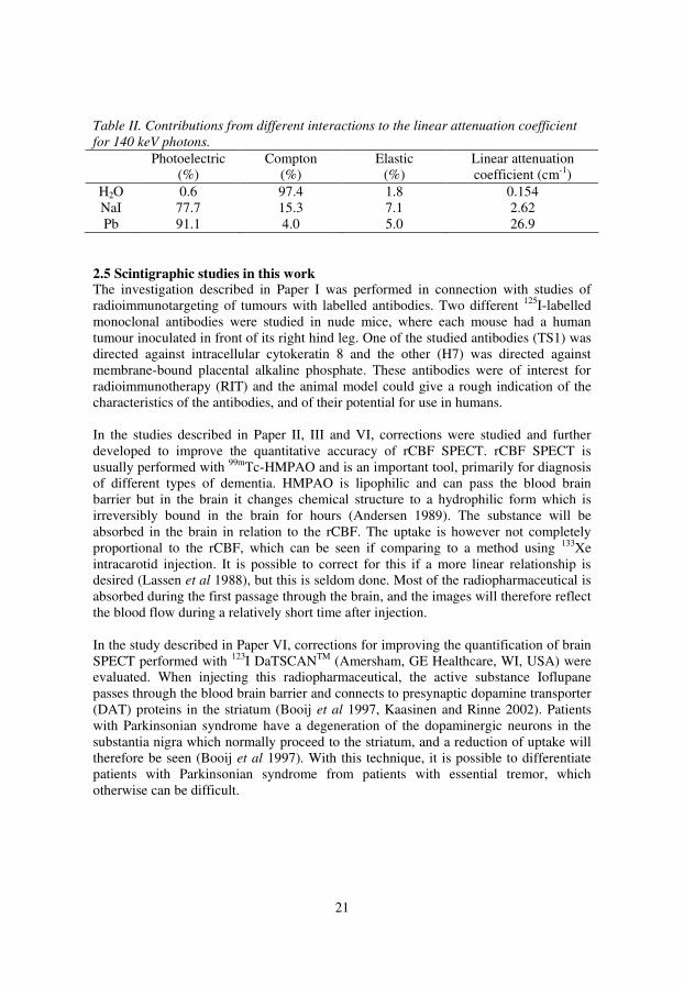
Table II. Contributions from different interactions to the linear attenuation coefficient

for 140 keV photons.

Photoelectric (%)

Compton (%)

Elastic (%)

Linear attenuation coefficient (cm-1)

H2O 0.6 97.4 1.8 0.154 NaI 77.7 15.3 7.1 2.62 Pb 91.1 4.0 5.0 26.9

2.5 Scintigraphic studies in this work The investigation described in Paper I was performed in connection with studies of radioimmunotargeting of tumours with labelled antibodies. Two different 125I-labelled monoclonal antibodies were studied in nude mice, where each mouse had a human tumour inoculated in front of its right hind leg. One of the studied antibodies (TS1) was directed against intracellular cytokeratin 8 and the other (H7) was directed against membrane-bound placental alkaline phosphate. These antibodies were of interest for radioimmunotherapy (RIT) and the animal model could give a rough indication of the characteristics of the antibodies, and of their potential for use in humans. In the studies described in Paper II, III and VI, corrections were studied and further developed to improve the quantitative accuracy of rCBF SPECT. rCBF SPECT is usually performed with 99mTc-HMPAO and is an important tool, primarily for diagnosis of different types of dementia. HMPAO is lipophilic and can pass the blood brain barrier but in the brain it changes chemical structure to a hydrophilic form which is irreversibly bound in the brain for hours (Andersen 1989). The substance will be absorbed in the brain in relation to the rCBF. The uptake is however not completely proportional to the rCBF, which can be seen if comparing to a method using 133Xe intracarotid injection. It is possible to correct for this if a more linear relationship is desired (Lassen et al 1988), but this is seldom done. Most of the radiopharmaceutical is absorbed during the first passage through the brain, and the images will therefore reflect the blood flow during a relatively short time after injection. In the study described in Paper VI, corrections for improving the quantification of brain SPECT performed with 123I DaTSCANTM (Amersham, GE Healthcare, WI, USA) were evaluated. When injecting this radiopharmaceutical, the active substance Ioflupane passes through the blood brain barrier and connects to presynaptic dopamine transporter (DAT) proteins in the striatum (Booij et al 1997, Kaasinen and Rinne 2002). Patients with Parkinsonian syndrome have a degeneration of the dopaminergic neurons in the substantia nigra which normally proceed to the striatum, and a reduction of uptake will therefore be seen (Booij et al 1997). With this technique, it is possible to differentiate patients with Parkinsonian syndrome from patients with essential tremor, which otherwise can be difficult.

22

3 QUALITY OF SCINTIGRAPHIC IMAGES

Image quality is often described using the basic parameters contrast, noise and spatial resolution. These parameters affect both the qualitative and quantitative evaluation of planar scintigraphic imaging and SPECT, and will be discussed below. The corrections applied for a quantitative evaluation will also affect these parameters in different manners and this is important to take into account when choosing between different correction methods. Image quality is heavily dependent on the performance of the gamma camera, and a detailed description of how to measure gamma camera performance can be found in the NEMA protocol (NEMA 2001), which sets a standard for definition and measurement of a number of quality parameters. A short description of the most important parameters for a quantitative evaluation will be discussed later in this section. Spatial resolution is an important quality parameter and will therefore be described as such.

3.1 Contrast Contrast is a measure of the difference in image intensity between adjacent regions in the image. The contrast in a planar image should ideally reflect a 2D projection of the activity distribution within the patient. In SPECT, the contrast is improved compared with a planar image, since there is no contribution from over- and underlying activity in the calculated 3D distribution of activity. In this case the contrast should ideally reflect the activity distribution in the different tissues. The contrast can however be influenced by attenuation, scatter, septal penetration and background radiation. For small objects, spatial resolution will also have a high impact on image contrast. Various equations for calculating contrast can be found in the literature. In the study described in Paper V, the following equation was used to calculate contrast, where N is the average value of registrations/pixel in the region of interest and B is the corresponding value in a surrounding background region:

%100⋅+

−=

BN

BNC (8)

3.2 Noise If an interaction in the NaI(Tl) crystal in the gamma camera is accepted to contribute to the image, one count will be added to the image pixel corresponding to the location of the photon interaction. Each pixel in the in the raw data image can therefore be viewed as a photon counter, and the probability of detecting x photons is then described by the Poisson distribution:

•

23

!)(

x

exxP

xx −

= (9)

where x is the expected number of detected photons (the mean value in a homogeneous region or in repeated identical measurements). The standard deviation of the Poisson distribution is calculated as:

xs = (10) If x is large, at least in the order of 15, the Poisson distribution can be approximated with a Gaussian distribution. Noise is usually calculated as a percentage as the standard deviation divided by the mean value. The limited amount of activity that can be given to the patient, the limited examination time and the construction of the collimator are factors that contribute to a high noise level in comparison with other diagnostic techniques. The noise level is often higher than 10% in SPECT projection images, but is in most cases lower in planar scintigraphic images due to the longer measurement time per image. The stochastic noise in the SPECT projection images will affect the noise level in the reconstructed images. After reconstruction, the noise is however non-stochastic and much more complex (Gillen 1992). The noise will be positively correlated at short distances and negatively correlated at long distances. The noise will then appear as “blobs” that can be of the same size as the information of interest, for example lesions, in the reconstructed images. The use of pre- or post filtering in the reconstruction process will of course affect the noise level, and a smoother filter will decrease the standard deviation, and increase the correlation length, that is make the noise blobs to appear larger (Rosenthal et al 1995). The MLEM and OSEM reconstruction algorithms take the Poisson noise into account, and furthermore, they don’t include the FBP ramp filter which amplifies high frequency noise. Images reconstructed using MLEM or OSEM should therefore have a higher signal-to-noise ratio compared with images reconstructed using FBP (Chornoboy et al 1990). If an iterative reconstruction like MLEM or OSEM is used, resolution and contrast increases with the number of iterations, but at the same time the noise level increases (Floyd et al 1987). A high noise level can be avoided by stopping the reconstruction at an early iteration step, application of a post-reconstruction filter, using compensation for CDR, or combinations of these. These options are discussed and compared in detail for myocardial imaging in the study by Hutton and Lau (1998), and they concluded that compensation for CDR is preferable to post-filtering. The noise level can also be decreased by low-pass filtering of the projections, as described in Paper II – III. That approach is more unusual but we found that it made it possible to use a comparably high number of iterations which gave a better contrast and spatial resolution than the corresponding post-filtering alternative would do for the same noise level. The CDR alternative, which is preferable, was used in the study described in Paper VI.

24

3.3 Quality parameters of a gamma camera 3.3.1 Spatial resolution

Spatial resolution is described by the full width at half maximum (FWHM) complemented by the full width at tenth maximum (FWTM) of the line spread function of the gamma camera system. It is measured in two perpendicular directions using a line source at a distance of 10.0 cm from the collimator surface, free in air or behind a scattering medium. Hereafter, only FWHM values of spatial resolution will be discussed. The spatial resolution in gamma camera imaging is generally rather poor in comparison with other radiological modalities. The limit of the spatial resolution is set by the intrinsic resolution, Ri, which should be near 3.5 mm for conventional crystal thicknesses and 140 keV photons, for modern gamma cameras (Hamilton 2004). It describes the ability of the system to transfer the spatial distribution of the absorbed energy in the crystal to a readable image (Strand 1998) and it depends primarily on the statistical fluctuation in the number of light photons hitting each PM-tube (Hamilton 2004). The spatial resolution of a gamma camera system is also heavily dependent on the collimator resolution Rc, and for a high resolution the collimator holes should be as long and narrow as possible. Rc is dependent on the distance from the collimator, and the value of Rc in mm increases in an approximately linear manner with increased distance for a parallel-hole collimator (Anger 1964). It is therefore important that the collimator is as close to the patient as possible during the examination. Spatial resolution is also dependent on scatter and septal penetration, to a less degree, and the contribution of these effects is called Rsc. The total spatial resolution can be calculated as (Strand 1998):

222scci

tot RRRR ++= (11)

Rtot is usually between 5 and 15 mm at a distance of 10 cm, depending on type of collimator, photon energy and if scatter is present or not. Spatial resolution will degrade because of patient movements, and different types of fixations may be needed to reduce such effects. Movements can also cause image artifacts. In the study described in Paper II, a thermoplastic face mask was used to reduce head movements, and this mask is also used in clinical practice for brain examinations at the Nuclear Medicine department in Umeå. The mask is formed individually for each patient and is fastened with VelcroTM-tapes underneath the head holder. It is demonstrated in Fig. 3.

•

25

Fig. 3. Thermoplastic face mask for brain examinations.

In SPECT, the resolution will depend on the resolution in the planar images, and of methods and possible filters used for reconstruction. The effect of the spatially varying resolution for different distances from the collimator will give asymmetric spatial resolution in the radial and tangential direction for off centre sources (Larsson 1980). This becomes more and more apparent the further away from the centre of rotation the source is located. 3.3.2 Sensitivity

Sensitivity is a measure of the number of photons detected for a certain amount of activity and a certain time, and it is usually measured in cps/MBq or cpm/µCi, where cps stands for “counts per second” and cpm for “counts per minute”. This factor must be known for an accurate absolute quantification of activity. Sensitivity is most dependent on the collimator, since it sets the acceptance angle for the incoming photons. It is also dependent on the crystal thickness, the exchange and energy of the incoming gamma photons and the width of the energy window. If septal penetration is low, the sensitivity is approximately constant with the distance to the detector for a parallel-hole collimator. To increase the sensitivity a collimator with a larger acceptance angle for the incoming photons can be used. This will decrease image noise at the expense of a worse spatial resolution. According to NEMA (2001) sensitivity should be measured during a specified time using a thin planar circular source of known activity of a diameter of 10 cm, 10 cm from the collimator surface. This sensitivity measurement includes some contribution from scatter, and a measure of sensitivity without scatter can be of interest for quantitative imaging. If a scatter free sensitivity is desired, sources with different diameters can been used, and the scatter contribution can been assumed to increase linearly with source area. The sensitivity can then be plotted against source area and the intercept with the y-

26

axis gives the sensitivity where scatter can be neglected (Sjögreen et al 2002). This sensitivity measurement may be valid also for the reconstructed SPECT-images (Ljungberg et al 2002). Different reconstruction programs can however normalise the reconstructed images in different ways, which has to be taken into account. If a separate sensitivity measurement has to be performed for quantitative SPECT, a point source or line source in air can be used and reconstructed with the same algorithm as in the patient study (Siegel et al 1999). The attenuation and scatter correction can however be omitted since the calibration is performed in air. 3.3.3 Uniformity

Uniformity is a measurement of sensitivity variations over the gamma camera surface. The sensitivity variations should be as low as possible, and this is especially important for a quantitative evaluation of the images since the degree of non-uniformity directly will appear in the quantitative values. Uniformity is an intrinsic measure, which means that it is measured without a collimator. The measurement is performed using a point source at a distance of at least 5 times the longest linear dimension of the NaI(Tl) crystal, to make an approximately parallel radiation field to the detector. A high number of counts is measured for a low noise level. The image is then subject to a few corrections. Operations are used to reduce the contribution from non-uniform edge-pixels and the whole image is low-pass filtered using a Gaussian filter kernel. Uniformity can then be calculated as:

%100minmax

minmax ⋅+

−=

NN

NNU (12)

where Nmax is the highest pixel value and Nmin is the lowest pixel value. For integral uniformity Nmax and Nmin are searched for in the whole field of view and for differential uniformity the maximal difference in Nmax and Nmin is searched for in five neighbouring pixels. Uniformity is most dependent on the PM-tubes and typical uniformity values range from 2-6% for modern equipment (Strand 1998). Uniformity is the most important quality parameter, and therefore it is also checked daily with a flood source, usually made of 57Co. These measurements are performed with the collimator on. Non-uniformities can be corrected for by using measured uniformity matrices. In SPECT, non-uniformities can appear as ring artifacts, showing the contribution from a mal-functioning PM-tube to the reconstructed image. The effects can be severe, especially if a central PM-tube is affected (Axelsson et al 1983). Uniformity corrections are therefore especially beneficial for SPECT.

•

27

3.3.4 Energy resolution

Energy resolution is also an intrinsic parameter and it is measured in a similar manner as uniformity. It can be calculated as:

0E

FWHMRE = (13)

where FWHM is the full width at half maximum of the photopeak, and E0 is the average energy of the peak. The energy resolution is approximately dependent on energy as

E/1 and typical values for modern equipment range from 8% to 10% for 140 keV photons (Strand 1998). The basic source of the poor energy resolution is the limited number of electrons hit loose at the photocathode of the PM-tubes, which gives a statistical uncertainty in the amplitude of the energy signal. Energy resolution is an indirect measure of the ability of the detector to discriminate scattered photons, since a better energy resolution means a better separation of the photopeak and Compton region. A good energy resolution makes it possible to use a smaller energy window and still maintain a high sensitivity. Typical sizes of energy windows are between 15% and 20% for 140 keV photons. 3.3.5 Count rate performance

The count rate performance is a measure of the ability of the system to reproduce the true count rate, which is the number of detected photons per time that would be within the energy window, if detected individually. Due to pulse pile-up, the camera is unable to respond to all detections in the crystal, and the observed count rate will therefore be less than the true count rate. This is important to take into account for an accurate quantification, and for count rates well below 100 000 cps it is possible to correct for this effect (Koral et al 1998). Count rate performance is measured as the maximum observed count rate and count rate at 20% losses. It is difficult to state typical values of these parameters, since large variations can be seen when comparing different gamma cameras. For the GE Millennium MG, simulated in the study described in Paper VI, the maximum observed count rate in a 15% energy window is specified to ≥ 220 000 cps and the value at 20% losses is specified to ≥ 155 000 cps. High count rates will lead to mispositioning of events and will have a negative effect on uniformity and spatial resolution (Hart 1992). The speed of the detector electronics has a great impact on count rate performance (Binkley and Young 1998).

28

4 QUANTITATIVE IMAGING

In SPECT and planar scintigraphic imaging, the images are in most cases evaluated qualitatively by visual inspection, but quantitative information related to the uptake of activity in different tissues can be of interest for various purposes. High accuracy quantification is however very difficult to achieve. One reason for this is the poor spatial resolution, which causes the so called “partial volume effect”. It means that objects of comparable size to the spatial resolution will be underestimated in terms of activity concentration, because of blurring. It has been stated that quantification will be unreliable for objects smaller than three to four times the system spatial resolution (Rosenthal et al 1995). In SPECT the distance dependent spatial resolution can be compensated for to some degree by using compensation for CDR, which is positive for a quantitative evaluation (Pretorius et al 1998). For an accurate quantification it is also necessary to correct for some other physical degrading factors, namely attenuation, scatter and in some cases also septal penetration. These factors affect image contrast by reducing the connection between image counts and activity concentration. Of these factors, attenuation is most important since the loss of counts due to this effect is substantial. For planar scintigraphic imaging, contribution of background counts from over- and underlying tissues must usually be corrected for (Siegel et al 1999). Factors related to the patient (for example motion and time-dependent tracer kinetics), technical factors (for example collimation, dead-time and non-uniformities) and procedural factors (for example pixel size, number of projections and reconstruction algorithm) must also be considered (Tsui et al 1994a, Rosenthal et al 1995). Quantification can be divided into two separate methods, absolute and relative quantification. 4.1 Absolute quantification Absolute quantification means to quantify the activity in the tissues of interest, and this is possible since the image counts are connected to activity by means of the system sensitivity. The activity within the tissues can then be compared with the injected activity for calculation of relative uptake. The relative uptake of activity in a specific organ or a tumour is a convenient quantitative measure, since it can be compared with other cases without taking differences in imaging systems and patient size into account (Rosenthal et al 1995). Absolute quantification is necessary for calculation of dose to different tissues. This is important when new radiopharmaceuticals are tested, and it is essential when evaluating risk and therapeutic effects of radiopharmaceuticals used for radionuclide therapy. The dose to a specific target organ in the body is calculated from the cumulated activity, which is the activity integrated over time (the total number of disintegrations). The cumulated activity in the organ itself is of course important for the dose calculation, but activity in surrounding tissues may also contribute to the dose. The cumulated activity depends on both uptake and retention of activity, and repeated activity measurements, with an appropriate sampling frequency, are required for a good approximation of the

•

29

activity integrated over time. The cumulated activity can then be calculated by curve-fitting and integration, numerical methods or compartmental modelling (Siegel et al 1999). One way of estimating dose to different tissues is by using the MIRD schema (Loevinger et al 1991), which has been used both for diagnostics and therapy (Stabin et

al 1999). According to the MIRD schema, the mean absorbed dose tD in a specific target organ in the body can be calculated as:

∑ ←=s st stSAD )(

~ (14)

where sA~

is the cumulated activity in the source organ. )( stS ← is the mean absorbed dose in the target organ per cumulated activity in the source organ, and depends on type of radiation, energies of the radiation involved and geometrical aspects of source and target regions (Loevinger et al 1991). S-values for different radionuclides can be found in tables for different pairs of source and target organs (Stabin 1996). In some cases no S-values exist, or the MIRD schema can be regarded as too approximate for individual dose estimation. In such cases, a voxel-based model based on CT or magnetic resonance tomography (MRT) images, together with Monte Carlo simulations, can be a possible alternative (Zaidi and Sgouros 2003). 4.1.1 Absolute quantification in this work

In the study described in Paper I, absolute quantification of the activity in the tumour inoculated in the flank of a mouse was of interest. Mice are the most commonly used animals for evaluation of new monoclonal antibodies with potential use for RIT, and a possibility to determine tumour activity in vivo over time is convenient in such studies. The monoclonal antibodies used in this study were labelled with 125I, and as can be seen in Table I the photons emitted when this radionuclide decays have relatively low energies. The average photon energy, weighted with the probability of emission, is 28.4 keV. On modern equipment the capability of measuring such low energies cannot be taken for granted since 125I is not used for imaging of patients, but it was possible on the analogue gamma camera used in this study. At Umeå University the mouse measurements have usually been performed with a pin-hole collimator. This type of collimator can provide a high spatial resolution if the pin-hole is small, and for the Porta Camera pin-hole collimator the hole diameter is 4.2 mm. The pin-hole collimator can also amplify the image of the mouse, which will reduce the effect of the poor intrinsic spatial resolution for the low photon energies on this piece of old equipment. However, the sensitivity will depend on the distance from the tumour to the pin-hole, which introduces uncertainties in the activity estimate. This requires a sensitivity calibration for the point where the tumour will be positioned. Attenuation and background correction was performed in this study, but scatter was not corrected for explicitly. The dose rate to the tumour, in units of Gy/(kBq·day), was

30

determined as a function of tumour mass for 125I using the nodule module of the MIRDOSE 3 program (Stabin 1996). The tumour was approximated to a small sphere with homogeneous activity distribution. Dose to the tumour from other tissues was neglected, and it was found that the contribution from electrons to the dose dominated completely. It should however be noted that if used for RIT in humans, the antibodies would probably have been labelled to some other radionuclide than 125I. 4.2 Relative quantification Relative quantification is a more “fuzzy” concept, and it means that quantitative information is derived from the counts in the image, and is compared to other data. In this case the calibration to activity is not necessary, but in most cases it is advantageous if the image counts are proportional to activity concentration, which requires corrections. The corrections needed for a relative quantification must however be considered from case to case, since there is no need to correct for effects that will cancel out in the comparison. Relative quantification can be used for comparison of counts between two different datasets, for example two different regions in the same image, but data in different images can also be compared. It can also mean comparison of images with normal or abnormal databases (Rosenthal et al 1995). 4.2.1 Relative quantification in this work

The rCBF images in this work were processed for relative quantification, to be used for research purposes. It has been shown that a normalisation of the reconstructed images to the well-established mean value of 50 ml/(100 g · min) increases the reproducibility significantly for 99mTc HMPAO rCBF SPECT measurements performed on the same subject (Jonsson et al 2000). This can for example depend on differences in the useful (lipophilic) part of the radiopharmaceutical, which can vary from vial to vial, but it can also depend on physiological factors (Jonsson et al 2000). Large variations in rCBF have also been observed when comparing different subjects (Devous et al 1986), and it seems clear that absolute quantification of 99mTc HMPAO rCBF SPECT is of little interest for diagnostics. Relative rCBF quantification is for example used when comparing groups of patients by using statistical software like SPM (Wellcome Department of Cognitive Neurology, London, UK) or CBA (Thurfjell et al 1995). This requires normalisation of uptake, but also a spatial normalisation to a standard space, so that all brains have the same size and shape. The importance of correction of physically degrading factors in such studies, especially scatter correction, has been demonstrated by Van Laere et al (2002). In our research group we have for example studied memory provoked rCBF SPECT on a group of patients with early Alzheimer’s disease and a group of healthy subjects (Sundström et al, in press). The subjects were examined twice, once after injection at rest and once after injection during face and name encoding (memory provocation). All images were corrected for attenuation and scatter. The memory provoked images from each group were compared with their corresponding resting state images by using SPM, and the two groups were also compared with each other. It was found that memory

•

31

provocation magnified group differences in rCBF and such a technique can therefore be positive for early diagnostics of Alzheimer’s disease. DAT studies are in most cases evaluated using relative quantification (Booij et al 1997, Parkinson study group 2000, Koch et al 2005) which should be mandatory for these studies (Tatsch et al 2002). Regions of interest (ROIs) are used for determining the number of counts in the striatum structures (left and right putamen and caudate nucleus) and one or more background regions, which should be placed occipitally or in the cerebellum (Tatsch et al 2002). Ratios of (striatum-background)/background counts can then be calculated and should preferably be compared with age-matched normal values. These ratios should in many cases be regarded as site-specific since differences in ROI-settings, equipment and reconstruction procedures can vary. Rough calibrations to ratios of the corresponding activity concentrations can however be performed using specially designed striatal phantoms. The quantitative accuracy is hampered by attenuation and scatter, and in most cases also septal penetration since these studies usually are performed with 123I-labelled compounds. The gain in quantitative accuracy when correcting for these effects has been shown for DAT studies and related studies (Hashimoto et al 1999, Almeida et al 1999, Soret et al 2003). It should however be noted that the contribution from septal penetration is called scatter in these references. Of great importance is the partial volume effect, because of the small size of the striatum structures, and a partial volume correction has been suggested (Soret et al 2003). In the study described in Paper VI, the images were corrected for attenuation, scatter, septal penetration and CDR.

32

5 THE MONTE CARLO METHOD

Monte Carlo simulations are based on sampling of random numbers to solve problems based on probability functions, and have been widely used in many fields in radiation physics (Andreo 1991). For nuclear medicine, simulations of photon transport have been shown to be useful for optimisation of detector design, development and evaluation of correction techniques, assessment of image reconstruction algorithms, ROC studies, modelling of tracer kinetics and assessment of absorbed dose (Buvat and Castiglioni 2002, Zaidi and Andreo 2003). Photon transport is relatively uncomplicated to simulate if the photon energy is low enough for the assumption of locally absorbed secondary electrons to be justified, and in scintigraphic imaging, this approximation is usually not a problem. A few Monte Carlo programs dedicated for gamma camera imaging have been developed, for example SIMIND (Ljungberg and Strand 1989), SimSPECT (Yanch et al 1992, 1993), MCMATV (Smith 1993, Smith et al 1993), SimSET (Harrison et al 1993) and recently GATE (Strul et al 2003). SimSET and GATE can also be used for PET. SimSPECT is based on the photon transport in the more general Monte Carlo code MCNP (Briesmeister 1986). Other general Monte Carlo codes have also been used with SPECT configurations, for example in the study by Narita et al (1996). They used EGS4 (Nelson et al 1985) for photon transport and interactions in the phantom, while a separate program modelled the gamma camera detection system. With Monte Carlo simulations it is possible to extract results that cannot be given by gamma camera measurements. It is for example possible to get statistics on important parameters for the different interactions in the object or the gamma camera, for example the number of scattering events, scattering angles and imparted energy (Ljungberg 1998a). Monte Carlo simulations are also very useful for studying the effect of different correction techniques, since it is possible to simulate images without a certain interaction type, for example scatter or septal penetration. This gives an ideal image without the effect of the studied interaction, which can be used for comparison with corrected images. For optimisation of different imaging systems, Monte Carlo simulations are useful since it is very simple to change different parameters in the system and study the difference in performance (Ljungberg 1998a). One has however always to bear in mind that simulations are based on computer models and are therefore approximations of real measurements, and that a perfect simulation of reality is very difficult to accomplish. For example, simplified models are sometimes used for interactions in different parts of the gamma camera to save computing time (Buvat and Castiglioni 2002). It is also important to note that the statistics of simulated gamma camera images may not be identical to the Poisson statistics in the corresponding measured images. This is due to the variance reduction techniques used to favour photon directions and events that will make them more likely to be detected, in order to reduce computing time. This is obtained using weights applied to the photon histories that represent the number of “real-world” particles represented by that history (Haynor 1998). Therefore, when a simulated photon is “detected”, the combined photon weight is added to the corresponding pixel, not one count as in a measurement. If

•

33

Poisson statistics is desired, virtually noise-free images can be simulated, and the effect of Poisson noise can then be added to the images. Simulated images can also be seen as ideal versions of reality since the patient never moves (if not specifically simulated) and imperfections in the detector system, for example non-uniformities, seldom are included. Scatter outside the studied object is also an effect which is usually not included in the simulations. 5.1 Monte Carlo simulations in this work The Monte Carlo method is used in this work as a tool for evaluation and optimisation of the correction methods. The simulations were performed with the SIMIND program (Ljungberg and Strand 1989, Ljungberg 1998b). The code is written in Fortran 90 and consists of two parts; CHANGE and SIMIND. In CHANGE, the simulated system is defined, and SIMIND performs the Monte Carlo simulation. The program follows each photon from its origin in the source to detection in the crystal. Phantoms and sources of standard shapes can easily be simulated, and it is also possible to use heterogeneous voxel-based phantoms developed from CT or MRT images. Two voxel-based heterogeneous phantoms have been used in this work for Monte Carlo simulations. One is a morphological phantom which includes various structures in the brain, whose densities and activity concentrations can be varied independently (Zubal et

al 1990, Zubal and Harrell 1992). This phantom will hereafter be called the “Zubal-phantom”. The other heterogeneous phantom was designed for comparing simulations and measurements of an RSD striatal phantom (Radiology Support Devices, CA, USA) in the study described in Paper V. This phantom includes five separate compartments where different activity concentrations can be added, and it was developed from CT images of the physical RSD striatal phantom used in the study. 5.1.1 Monte Carlo simulations of collimator interactions

The SIMIND version used for simulations in the studies described Paper II-IV includes collimator specifications to calculate spatial resolution, but it does not take interactions in the collimator into account when producing the images. This approximation is not a problem for radionuclides emitting gamma photons of low energy, such as 99mTc, since septal penetration is negligible for low photon energies and since the cross section for photoelectric absorption for the collimator material (lead) is much higher than the scatter cross section (which can be seen in Table II). For radionuclides that also emit high energy photons, such as 123I, it is however a serious approximation not to take septal penetration and scatter in the collimator into account (de Vries and Moore 1998, Song et al 2005). A code that simulates photon transport in the collimator has been developed by de Vries et al (1990) and it has been adapted for use with SIMIND. This code is based on rectangular collimator holes, and if the simulated collimator has hexagonal holes, adjustments of the hole size and septal thickness may be needed to make simulated and measured images to correspond, approximately (Dewaraja et al 2000).

34

The code described in Paper V, developed by Michael Ljungberg, is based on hexagonal collimator holes. This means that no adjustment to the collimator geometry is needed for most collimators, since most collimators are built this way. Adjustments might however be needed for the backscattering layer behind the crystal, which is an approximation of the PM-tubes and electronics behind the crystal which scatters some of the high energy photons back into the crystal. A layer of 4.0 cm Lucite was found to be appropriate for the MPR gamma camera used in this study. The photon transport in the collimator is based on the Delta-Scattering technique (Woodcock et al 1965). This is a statistical method that doesn’t require time consuming ray-tracing through a heterogeneous grid of media. The technique is therefore advantageous for simulations of collimators with hexagonal holes since their geometry is relatively complex. In this case the path-lengths through the collimator Pn are sampled from

max

)ln(

µn

n

RP

−= (15)

where Rn is a random number between 0 and 1 and µmax is the largest attenuation coefficient of the heterogeneous media. According to the Delta-Scattering technique, a secondary random number is sampled at the endpoint of the path. This random number is compared with the ratio of µ/µmax, where µ is the attenuation coefficient at that point. If the random number is less than this ratio, the point is considered to be a place of interaction. Otherwise the photon continues with a new path-length according to Eq. 15. In this case the collimator only consists of two materials, air and lead. The attenuation coefficient of air is approximated to 0, and the ratio will therefore be either 0 or 1. It is therefore only required to test whether or not the endpoint of a path is within a collimator hole. This is tested for each path endpoint by using equations based on the hexagonal hole geometry. If the endpoint is not within a hole, it must be in the septa between the holes, and an interaction is simulated. This program was evaluated for 123I in the study described in Paper V by comparing simulations with real measurements for two collimators; low energy general purpose (LEGP) and low energy high resolution (LEHR). Point sources at different distances from the collimator were used, and we also used the RSD striatal phantom described earlier. Both images and energy spectra were compared and a good correspondence was found. In recent versions of SIMIND the Delta-Scattering technique is also used to simulate photon transport within a heterogeneous voxel-based phantom.

•

35

6 CORRECTIONS FOR QUANTITATIVE SPECT 6.1 Attenuation correction Attenuation correction is the correction for the loss of counts in the images, due to attenuation in the patient. Photoelectric absorption is an obvious source of attenuation that needs correction, but the primary interaction process in tissue for photons from radionuclides used for scintigraphic imaging is Compton scattering (which can be seen in Table II for 140 keV photons). Most of the Compton scattered photons will not be detected because of out-scattering from the patient, photoelectric absorption in the patient or energy discrimination in the gamma camera. The scattered photons that are detected contain less useful information and can be corrected for using techniques described in the next section. Attenuation will be referred to as the loss of useful counts and scatter as the addition of unwanted counts in this work. The equation describing the attenuated SPECT projections from a source distribution f(x,y) in an attenuating medium is called the attenuated Radon transform, and can be written as:

drdlyxyxfsp

sL

yxl

∫ ∫

−=

),(

),(

0

)','(exp),(),(θ

µθ (16)

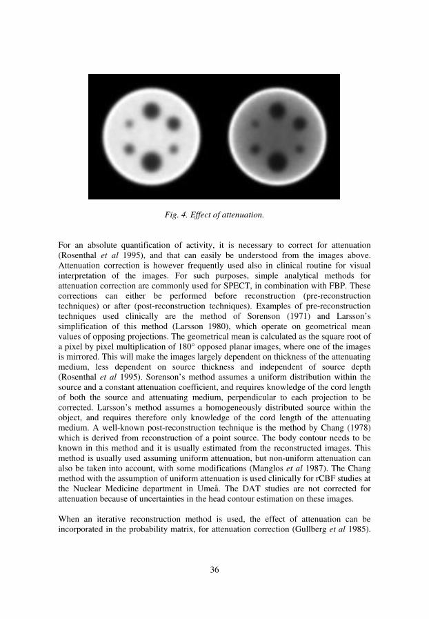
where p(s,θ) is the 1D projection data for the camera angle θ, l(x,y) is the distance from the emission point (x,y) to the detector along the line L(s,θ) and µ is the spatially variant attenuation coefficient (Zaidi and Hasegawa 2003). One would like to solve this equation for f(x,y), and inversions for this equation have been developed during the last years (Novikov 2002, Natterer 2001). They are however not of widespread use. A demonstration of the effect of attenuation in SPECT can be seen in Fig. 4, for a cylindrical 99mTc-water phantom, containing six spheres of water without activity, with diameters from 1.34 cm to 3.80 cm (a “Jaszczak phantom”). The diameter of the phantom is 20 cm. The projection images are simulated using SIMIND, with parameters corresponding to the Neurocam shown in Fig. 2 b, equipped with LEHR collimators. In the left image, no interactions were allowed in the phantom and in the right image attenuation, but not scatter, was included which means that a perfect energy resolution was simulated. The 64 projection images were reconstructed using OSEM with 12 iterations, 4 projections/subset, and were corrected for CDR but not attenuation. It can be seen that attenuation leads to an underestimation of the activity concentration, especially in the centre of the phantom. For more complicated density and activity distributions, image artifacts and distortions can be induced (Tsui et al 1989).

36

Fig. 4. Effect of attenuation.

For an absolute quantification of activity, it is necessary to correct for attenuation (Rosenthal et al 1995), and that can easily be understood from the images above. Attenuation correction is however frequently used also in clinical routine for visual interpretation of the images. For such purposes, simple analytical methods for attenuation correction are commonly used for SPECT, in combination with FBP. These corrections can either be performed before reconstruction (pre-reconstruction techniques) or after (post-reconstruction techniques). Examples of pre-reconstruction techniques used clinically are the method of Sorenson (1971) and Larsson’s simplification of this method (Larsson 1980), which operate on geometrical mean values of opposing projections. The geometrical mean is calculated as the square root of a pixel by pixel multiplication of 180° opposed planar images, where one of the images is mirrored. This will make the images largely dependent on thickness of the attenuating medium, less dependent on source thickness and independent of source depth (Rosenthal et al 1995). Sorenson’s method assumes a uniform distribution within the source and a constant attenuation coefficient, and requires knowledge of the cord length of both the source and attenuating medium, perpendicular to each projection to be corrected. Larsson’s method assumes a homogeneously distributed source within the object, and requires therefore only knowledge of the cord length of the attenuating medium. A well-known post-reconstruction technique is the method by Chang (1978) which is derived from reconstruction of a point source. The body contour needs to be known in this method and it is usually estimated from the reconstructed images. This method is usually used assuming uniform attenuation, but non-uniform attenuation can also be taken into account, with some modifications (Manglos et al 1987). The Chang method with the assumption of uniform attenuation is used clinically for rCBF studies at the Nuclear Medicine department in Umeå. The DAT studies are not corrected for attenuation because of uncertainties in the head contour estimation on these images. When an iterative reconstruction method is used, the effect of attenuation can be incorporated in the probability matrix, for attenuation correction (Gullberg et al 1985).

•

37

This is preferable for accurate quantitative imaging (Tsui et al 1989, Chornoboy et al 1990). The attenuation information required by this process is in the form of a 3D attenuation map, which describes the varying linear attenuation coefficient within the examined part of the body. If the studied part of the body has approximately homogeneous attenuation characteristics, as for example the abdomen or the brain, a uniform attenuation map can be used without too much loss of accuracy (Zaidi and Hasegawa 2003). In theory, it is however always an advantage to take the varying attenuation coefficient into account. Non-uniform attenuation maps are especially beneficial for the heart- and lung region where the attenuation coefficient varies due to the low density of the lungs and the high density of the spine (Tsui et al 1989, Ficaro et

al 1996). It is however important to take the possibility of artifacts in the attenuation map into account and quality control of attenuation maps is essential for ensuring the accuracy of the corrected images (Celler et al 2005). The most reliable method to determine non-uniform attenuation maps is by using transmission measurements with either a radionuclide or a CT scanner (Zaidi and Hasegawa 2003). There are however examples of methods that try to determine non-uniform attenuation maps from the emission data by using segmentation techniques (Wallis et al 1995, Pan et al 1997). 6.1.1 Transmission measurements with a radionuclide

Transmission measurements can be performed to give a direct measurement of the attenuation characteristics within the patient. The maps are acquired in a manner analogous to SPECT, with a rotating gamma camera and reconstruction to a 3D image volume. A blank scan, without the patient present, is also required. The relation between the pixel values in the acquired transmission images t(d) and the blank scan b(d) can be described as:

))(exp()()( ∫−=L

dxxdbdt µ (17)

where L is the path from the source to the detector (Vandenberghe et al 2001) and µ(x) is the spatially varying attenuation coefficient. A logarithmic operation gives the Radon transform r(d) of the attenuation map according to:

)(

)(ln)(

dt

dbdr = (18)

The attenuation map can then be reconstructed using FBP or iterative techniques (Vandenberghe et al 2001). The use of transmission measurements with radionuclides for non-uniform attenuation correction in SPECT started in the mid-1980s (Morozumi et al 1984, Malko et al 1986). The same radionuclide can be used for both the transmission measurement and emission

38

measurement, but for practical reasons a long lived isotope is used in most cases (Zaidi and Hasegawa 2003). Examples of radionuclides used commercially for transmission measurements in SPECT are 241Am, 153Gd, 195Au, 57Co and 133Ba (Ogawa 2004). Because of the difference in emission and transmission photon energies, the measured attenuation coefficients must be scaled to match the emission radionuclide. The transmission measurement should preferably be performed in direct connection to the emission measurement and can be performed before, during or after the emission scan (Bailey 1998). Different source geometries can be used for transmission measurements, and the collimation of the detector opposing the source must match the photon direction. Planar sources (Malko et al 1986, Tsui et al 1989), scanning line sources (Tan et al 1993) or multiple collimated line sources (Larsson et al 1993, Celler et al 1998) can be used together with parallel-hole collimators. Planar sources have certain drawbacks (Bailey 1998). Significant cross-talk registrations from down-scatter from the emission photons to the transmission energy window will occur. Furthermore, the measured attenuation coefficients will be “effective” attenuation coefficients because of detection of scattered transmission photons. This effect can be reduced by collimation of the planar source (Tsui et al 1989), and that will also reduce the dose to the patient. For the scanning line source, the gamma camera can be electronically windowed to only measure registrations in a region corresponding to the line in the image. This reduces the number of cross-talk registrations between the emission and transmission scans, and fewer scattered transmission photons are detected. A disadvantage with this system can be synchronisation problems with the mechanical motion and the electronic windows (King and Farncombe 2003). The multiple line source system by Celler et al (1998) includes correction for cross-talks and they have reported a better agreement than 96% of measured and true attenuation coefficients. Geometries with other types of collimators are reviewed in the studies by Bailey (1998) and Zaidi and Hasegawa (2003). The activity of the transmission source is limited, and relatively long measurement times are required for transmission images with a low noise level. The low noise level is important since the noise in the transmission scan otherwise will increase the noise level in the corrected emission data. To avoid long measurement times, segmentation can be performed where the noisy reconstructed transmission images are segmented into groups of pixels corresponding to different anatomical regions with uniform attenuation (Meikle et al 1993, Takahashi et al 2004). Takahashi et al (2004) reported a speed up factor of 5 for measuring an attenuation map for myocardial SPECT by using this method. This technique requires however further investigation. The problems with attenuation map artifacts have mainly concerned transmission systems with radionuclides. Problems with missing counts in the transmission images, down-scatter of emission photons in the transmission energy window and truncation of attenuation maps have for example been reported (Celler et al 2005).

•

39

6.1.2 Transmission measurements with a CT scanner

CT images are based on attenuation of bremsstrahlung photons from an X-ray tube. The photon energies are therefore distributed in a spectrum with a considerably lower average energy compared with the photon energies for most radionuclides used for scintigraphic imaging. The CT scanner measures a number of attenuated profiles around the patient, which in most cases are reconstructed using FBP. The attenuation information is recalculated to a standard scale, Hounsfield numbers (H), by this equation (Curry, III et al 1990):

w

wHµ

µµ −=1000 (19)

where µ is the attenuation coefficient in the voxel of interest and µw is the attenuation coefficient of water for the X-ray photons in average. To be used for attenuation correction in SPECT, the Hounsfield numbers must be calibrated to the attenuation coefficients of the SPECT radionuclide. This conversion is not uniquely defined since attenuation coefficients depend both on electron density and atomic number. A reasonably accurate approximation can however be achieved (Fleming 1989). For Hounsfield numbers below that of soft tissue, tissue can be assumed to be a mixture of soft tissue and air, and for higher Hounsfield numbers tissue is can be seen as a mixture of soft tissue and bone (Zaidi and Hasegawa 2003). This gives a straightforward calibration for the Hounsfield numbers below that of soft tissue since we have two fix points in the scale, air and water, where we know the Hounsfield numbers and their corresponding radionuclide attenuation coefficients. A linear relationship is usually assumed between these points. This linear relation can however not accurately describe the attenuation coefficients in bone for most radionuclides (LaCroix et al 1994) since photoelectric absorption is more important for the X-ray photons in comparison with the higher energy emission photons. The probability of attenuation in bone will therefore increase more for the X-ray-photons than for the emission photons due to the Z-dependence in Eq. 3. It is therefore advantageous to do a calibration for the Hounsfield numbers above that of soft tissue. An example of such a calibration can be seen in the study by Blankespoor et al (1995). They used a phantom with tissue equivalent materials with known chemical compositions. The resulting calibration curve is specific for each kVp setting on the CT scanner, and each setting requires its own calibration. The CT image volume must then be registered to the SPECT image volume, which means geometrical operations, including scaling, to make the two image volumes to correspond. After registration, each voxel in the CT image volume should point to the same piece of anatomy as the voxel with corresponding coordinates in the SPECT image volume. A number of different registration methods have been developed. For example, fiducial markers on the patient can be used in both modalities, but registration can also be performed by using different anatomical landmarks or methods based on voxel intensities (Hutton 2002).

40

Modern SPECT/CT hybrid cameras have been developed, and for these systems registration is not problematic if the patient stays on the table in the same position for the two measurements. If images from a conventional CT scanner are used, registration is a challenge since the patient position can differ in all three dimensions, and the flexing and bending of different body parts can be different. In most cases the body is however approximated to be a rigid object, since this is the simplest technique (Sjögreen 2001). In this case the registration is performed using three parameters for translation and three parameters for rotation. For the brain, different registration procedures using this approximation have been shown to be quite successful, since the head is a relatively rigid part of the body (Zaidi and Hasegawa 2003). CT image-based attenuation maps have a high spatial resolution and a low noise level compared with attenuation maps measured using transmission measurements with radionuclides. A dedicated CT scanner gives however a relatively high dose to the patient, and the use of CT measurements for attenuation correction purposes only can of course be questioned as a routine basis for diagnostic imaging. The X-ray tubes in some SPECT/CT hybrid cameras operate however on a lower dose-level compared with a dedicated CT scanner, and the acquired CT images are also used for other purposes than attenuation correction. When used for image fusion, they give the anatomical localisation of the functional information, and can therefore improve the diagnostics also in that way (Schillaci et al 2004). 6.1.3 Attenuation correction in this work

In the study described in Paper II, a method for attenuation and scatter correction of brain SPECT based on CT images of the same patient was developed and evaluated. The method is based on non-uniform attenuation maps, calculated from CT images, which are used by the iterative reconstruction program (OSEM). The CT images are acquired on dedicated CT scanners and the Hounsfield numbers are converted to linear attenuation coefficients for the photons emitted by the radionuclide. The CT images were acquired on a LightSpeed QX/i (General Electric, WI, USA) or a Somatom Plus 4 Power (Siemens, Germany) machine. The calibration for Hounsfield numbers above that of soft tissue was performed using a part of a fresh cow thigh-bone, from which the marrow had been removed. The bone density was determined and the average Hounsfield number was calculated for both CT scanners used in the study, for 120 kVp. An uncertainty in this case is of course a possible difference in bone composition between cows and humans. The calibration curve for the 140 keV photons emitted by 99mTc is shown in Fig. 5.

•

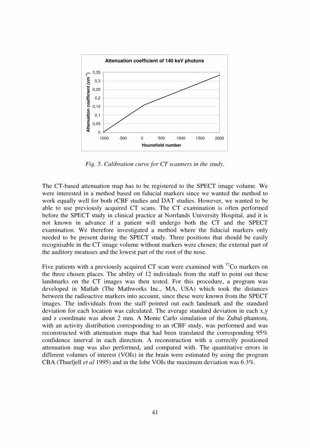
41

Attenuation coefficient of 140 keV photons

0

0,05

0,1

0,15

0,2

0,25

0,3

0,35

-1000 -500 0 500 1000 1500 2000

Hounsfield number

Att

en

ua

tio

n c

oe

ffic

ien

t (c

m-1

)

Fig. 5. Calibration curve for CT scanners in the study.

The CT-based attenuation map has to be registered to the SPECT image volume. We were interested in a method based on fiducial markers since we wanted the method to work equally well for both rCBF studies and DAT studies. However, we wanted to be able to use previously acquired CT scans. The CT examination is often performed before the SPECT study in clinical practice at Norrlands University Hospital, and it is not known in advance if a patient will undergo both the CT and the SPECT examination. We therefore investigated a method where the fiducial markers only needed to be present during the SPECT study. Three positions that should be easily recognisable in the CT image volume without markers were chosen; the external part of the auditory meatuses and the lowest part of the root of the nose. Five patients with a previously acquired CT scan were examined with 57Co markers on the three chosen places. The ability of 12 individuals from the staff to point out these landmarks on the CT images was then tested. For this procedure, a program was developed in Matlab (The Mathworks Inc., MA, USA) which took the distances between the radioactive markers into account, since these were known from the SPECT images. The individuals from the staff pointed out each landmark and the standard deviation for each location was calculated. The average standard deviation in each x,y and z coordinate was about 2 mm. A Monte Carlo simulation of the Zubal-phantom, with an activity distribution corresponding to an rCBF study, was performed and was reconstructed with attenuation maps that had been translated the corresponding 95% confidence interval in each direction. A reconstruction with a correctly positioned attenuation map was also performed, and compared with. The quantitative errors in different volumes of interest (VOIs) in the brain were estimated by using the program CBA (Thurfjell et al 1995) and in the lobe VOIs the maximum deviation was 6.3%.

42

In the studies described in Paper III and VI, attenuation correction was included but not a subject of investigation. The attenuation maps were calculated from the density maps used by the Monte Carlo program and were included in the OSEM reconstructions.

6.2 Scatter correction Scatter correction of scintigraphic images usually means correction for detected Compton scattered photons. It is less important to correct for elastic scattering since this interaction process is much less likely to occur than Compton scattering, and since its scattering angles generally are smaller. Most of the detected scattered photons have scattered in the patient, but scattering from other parts of the detector system and its environment can also be detected. The amount of scattered registrations depends on the size, density and composition of the studied part of the patient, and the distribution of the radiopharmaceutical within that part of the body. Furthermore, it depends on photon energy, the energy resolution of the gamma camera and the size of the energy window used. A smaller window, perhaps also centred asymmetrically, reduces the number of scattered registrations at the expense of reduced sensitivity. Most of the detected scattered photons have scattered only once, but photons having scattered 2 or 3 times will also contribute to the number of scattered registrations (Zaidi and Koral 2004). Detected scattered photons carry false information about their emission sites, since their place of detection in the crystal does not correspond to the projected place of emission. This is illustrated in Fig. 6, where a profile of the registrations from a small spherical source in a rectangular water phantom is shown. Scatter will therefore reduce image contrast, but artifacts can also be induced, for example in cardiac imaging (King et al 1996). These effects will reduce the quantitative accuracy. The effect of scatter in SPECT is demonstrated in Fig. 7 for the same water phantom as shown in Fig. 4. For the left image, both attenuation and scatter were allowed in the simulation, but for the right image only attenuation was allowed. Both images are corrected for attenuation, and for the left image an effective attenuation coefficient of 0.12 cm-1 was used, while the linear attenuation coefficient 0.154 cm-1 for the 140 keV photons was used for the right image. The attenuation correction was performed using a uniform attenuation map as input to the OSEM reconstruction. The reduction in contrast in the image including scatter can clearly be seen in the spheres without activity. The attenuation correction method described above, which uses an effective attenuation coefficient to deal with the scattered registrations, is very common clinically. It prevents an overcompensation of attenuated photons. More advanced methods are however needed to correct for the reduction in contrast and possible artifacts, which is important for a quantitative evaluation (Zaidi and Koral 2004). A variety of scatter correction techniques have been developed and evaluated. Many methods are based on subtraction of scatter images. The scatter images can be for example be estimated from measurements in more than one energy window or from convolution with scatter functions. A more modern approach is to include scatter correction in the iterative

•

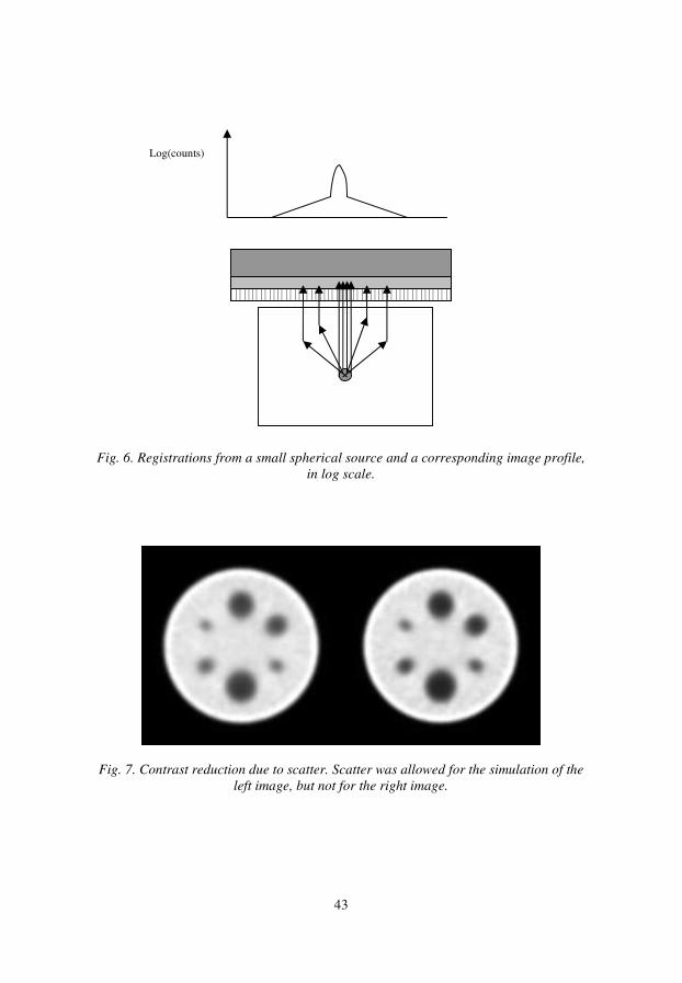
43

Fig. 6. Registrations from a small spherical source and a corresponding image profile,

in log scale.

Fig. 7. Contrast reduction due to scatter. Scatter was allowed for the simulation of the

left image, but not for the right image.

Log(counts)

44

reconstruction, to include 3D information when modelling scatter. In this work, only a few of all methods developed for scatter correction will be discussed. A broader selection can be found in the reviews by Buvat et al (1994) and Zaidi and Koral (2004). It should however be noted that all scatter correction methods are based on approximations, and severe approximations may introduce image artifacts. Furthermore, corrections based on subtraction of scatter images increase image noise, more or less, and methods included in iterative reconstructions can demand a lot of computing time. Many methods are not yet fully evaluated. These factors are probably the main reasons for the slow introduction of scatter correction into clinical practice. The author’s view is however that scatter correction is beneficial not only for a quantitative evaluation but also for visual interpretation of the images, and that this potentially very useful correction is not used to its full advantage today. 6.2.1 Energy window techniques

A variety of different energy window techniques for scatter correction exist but only the three most commonly used will be presented here. A classic example is the Compton window method (Jaszczak et al 1984) where images are acquired at the same time in the photopeak window and a Compton window. A fraction of the Compton window image is then subtracted from the photopeak image to give the corrected image. The assumption of identical spatial distribution of scatter in the two windows is however an approximation that doesn’t take the difference in scattering angles and multiple scattering into account. The method was originally developed for operating on the reconstructed images, but it can be used for the projection images as well (Mas et al 1989). Another example is the dual photopeak window technique (King et al 1992). In this method the photopeak is divided into two non-overlapping windows, symmetrically located around the centre of the photopeak. More scattered registrations appear in the lower window compared with the upper window, and the total number or scattered registrations to subtract is calculated from a power function including the registrations in the lower window divided by the registrations in the upper window. A popular method is the triple-energy window technique (TEW) introduced by Ogawa et al (1991). The method is illustrated in Fig. 8. TEW is based on two small subwindows adjacent to the photopeak window, one at each side of the photopeak. The scatter image to subtract, g(x,y)sc, is approximated by the triangular grey-shaded area in Fig. 8, which is calculated as:

2

),(),(),( p

s

right

s

left

sc

W

W

yxg

W

yxgyxg

+= (20)

g(x,y)left and g(x,y)right are the number of counts in the left and right subwindows which have the width Ws, and Wp is the width of the photopeak. If downscatter from higher

•

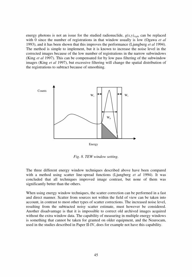
45

energy photons is not an issue for the studied radionuclide, g(x,y)right can be replaced with 0 since the number of registrations in that window usually is low (Ogawa et al 1993), and it has been shown that this improves the performance (Ljungberg et al 1994). The method is simple to implement, but it is known to increase the noise level in the corrected images because of the low number of registrations in the narrow subwindows (King et al 1997). This can be compensated for by low pass filtering of the subwindow images (King et al 1997), but excessive filtering will change the spatial distribution of the registrations to subtract because of smoothing.

Fig. 8. TEW window setting.

The three different energy window techniques described above have been compared with a method using scatter line-spread functions (Ljungberg et al 1994). It was concluded that all techniques improved image contrast, but none of them was significantly better than the others. When using energy window techniques, the scatter correction can be performed in a fast and direct manner. Scatter from sources not within the field of view can be taken into account, in contrast to most other types of scatter corrections. The increased noise level, resulting from the subtracted noisy scatter estimate, must however be considered. Another disadvantage is that it is impossible to correct old archived images acquired without the extra window data. The capability of measuring in multiple energy windows is something that cannot be taken for granted on older equipment, and the Neurocam, used in the studies described in Paper II-IV, does for example not have this capability.

Energy

Wp

Counts Ws Ws

46

6.2.2 Convolution techniques

Scatter corrections based on convolution or deconvolution were introduced by Axelsson et al (1984) as a 1D method which was further developed to 2D by Msaki et al (1987). These methods take the spatial distribution of the scattered photons into account instead of the energy spectra. The methods operate on geometrically mean valued images to decrease the depth dependence. A scatter kernel describes the spatial distribution of the scattered photons, which in most cases, but not always (Narita et al 1996), is assumed to have monoexponential form. The exponential describing the fall-off of the scatter kernel is called “slope” in this work. Methods based on deconvolution use a one-step operation to calculate the scatter corrected image (Floyd et al 1985, Msaki et al 1987) whereas methods based on convolution can be seen as two-step operations (Axelsson et al 1984). For the 2D two-step operation, convolution scatter subtraction (CSS), the geometric mean valued image of primary registrations g(x,y) can ideally be calculated as (Msaki et

al 1993):

)),((),(),( syxgkyxgyxg Pobs ⊗−= (21) where gobs is the observed, non-corrected geometrically mean valued projection image, kp is the scatter-to-primary ratio and s is the stationary scatter kernel. In this equation the image of primary registrations appear on both sides, and an approximation is therefore used where the original image is convolved with the scatter kernel:

)),((),(),( syxgkyxgyxg obsTobs ⊗−= (22) kT in this equation is the scatter-to-total ratio. The method is based on the approximation that both the scatter-to-total ratio and the slope of the scatter kernel are constant. For a uniform object such as a cylindrical water phantom with uniform activity, this approximation is not too serious, but the severity of the approximation will increase for more inhomogeneous source distributions and density variations (Msaki 1994). The transmission dependent convolution subtraction (TDCS) method (Meikle et al 1994) was developed from CSS. Instead of using a global scatter fraction as for CSS, a scatter fraction is calculated for each pixel in the image to be corrected. In this way one of the stationary factors in CSS is removed. The scatter fractions can be calculated from transmission measurements but they can also be calculated from ray sums through an attenuation map obtained by some other method, for example from CT images. This scatter correction technique can therefore easily be implemented if a non-uniform attenuation correction is utilised. The corrected image is calculated as:

)),()(,(),(),( syxgyxkyxgyxg obsTobs ⊗−= (23) where kT(x,y) is the matrix of scatter-to-total ratios. These can be calculated as (Meikle et al 1994):

•

47

2/)(1

1),(βα y)t(x,A

11

dBC

CCyxk

b

nbT

−−=−=

−= (24)

Cb is the number of broad beam counts, Cn are the narrow beam counts, B(d) is the depth-dependent build-up factor, A, α and β are empirical constants (Meikle et al 1991) and t(x,y) is the matrix of narrow beam transmission factors. TDCS has been shown to give quantitative results with an accuracy better than 95% in the heart and lung region in a thorax phantom (Meikle et al 1994). Quantitative results that are more accurate than results obtained using the TEW scatter correction technique and with a higher signal to noise ratio have also been demonstrated for simulations and measurements of a chest phantom (Narita et al 1996). The primary source of weakness lies in the fact that it is a 2D method with a scatter kernel that is independent on object thickness and source distribution. The composition and shape of the object can however be taken into account to some degree because of the spatially varying scatter-to-total ratio. 6.2.3 Scatter correction in an iterative reconstruction procedure

When scatter correction is included in the iterative reconstruction procedure it is possible to take 3D information of the patient into account. The scattered photon can actually be mapped back to the point of origin of the primary photon, which leads to a lower noise level compared with subtraction of scatter images (Frey et al 1992). For MLEM and OSEM, the scatter estimation can be included in both the projection and back-projection step in Eq. 2. It has however been shown that it is possible to get accurate results if scatter only is included in the projection step and this saves computing time (Kamphuis et al 1998). Even more time-saving techniques have been investigated where scatter simply is added as an extra term in the projection step (King et al 1997, Hutton and Baccarne 1998). The modelling of scatter in iterative reconstruction techniques can be performed with different degrees of complexity. A fast and relatively simple approach is described by Frey and Tsui (1993) where a slab-derived scatter estimation (SDSE) is used. The method was originally developed for 2D reconstructions but can easily be extended to 3D (Frey and Tsui 1993). Scatter line spread functions (SLSF) which describe the distribution of scatter from a line source were simulated at different distances from the collimator and at different depths in a rectangular water phantom. The results were parameterised and stored in tables. The scatter estimate can be adjusted to some degree for complex object shapes in this method. A disadvantage is that the technique cannot take a non-uniform attenuation map into account and is therefore not suitable in for example the heart and lung region. This model has later been improved to a technique called ESSE, effective source scatter estimation (Frey and Tsui 1996). In this method the scatter component at a certain projection position is calculated as the attenuated profile of an effective scatter source. The method is rather complex. A 3D “effective source scatter kernel” and a 3D “relative scatter attenuation kernel” are combined to give three kernels which are filtered with the

48

activity distribution, in the frequency plane, in 3D. A linear combination of these filtered image volumes gives the image volume which is called the effective scatter source. The attenuated profile of this image volume gives the scatter estimate. The method can be included in both the projection and backprojection step, or in the projection step only. In the ESSE model both the effective source scatter kernel and the scatter attenuation kernel are invariant. The model can therefore not take the effect of the non-uniform attenuation into account when calculating the probability of reaching the last scatter point. It can however take the non-uniform attenuation into account between the last scatter point and the detector. The model is therefore expected to work less well for non-uniform objects and can have errors near the edge of the object (Frey and Tsui 1996). Nevertheless, the model has shown good correspondence to Monte Carlo simulations (Frey and Tsui 1996). The maximum level of complexity for scatter corrections included in the iterative reconstruction, which should give the most accurate result, is the use of Monte Carlo simulations to compute the probability matrix. The technique is called inverse Monte Carlo and was first evaluated by Floyd et al (1986) for SPECT. They also included attenuation correction and CDR compensation in their 2D model. A complete 3D modelling procedure would however be much too time consuming to be practical in clinical work. Attempts have however been made to make the method more effective. Beekman et al (2002) have developed a technique based on Monte Carlo simulations, which is orders of magnitude faster than the original idea. The technique models scatter only in the projection step, uses fewer photon histories in early iterations, reuses photon tracks and uses an analytic detector modelling, all to reduce computing time. The reported reconstruction time for a 3D reconstruction is only 30 minutes on a 1.4 GHz computer. 6.2.4 Scatter correction in this work

The scatter correction method that is most focused upon in this work is TDCS, and it has been used with a monoexponential kernel. In the study described in Paper II, TDCS was used for scatter correction of 99mTc rCBF SPECT. The transmission factors in Eq. 24 are usually derived from transmission measurements, but in the study described in Paper II, CT-based attenuation maps were used for attenuation correction. We therefore calculated the transmission factors to be used for TDCS from ray sums through the CT-based attenuation maps. This technique should have better noise characteristics compared with the technique based on transmission measurements, since a projection through a CT-based attenuation map is almost free from noise, which is not the case for a transmission measurement with a radionuclide. A CT-based attenuation map has however a comparably high spatial resolution and multiplication by CT-derived transmission factors will therefore introduce a high frequency component to the scatter estimate. This is probably not of great importance since the CT-based attenuation map has been downsampled to match the SPECT matrix size, but it should perhaps be investigated further.

•

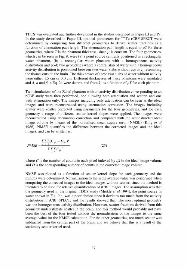
49

TDCS was evaluated and further developed in the studies described in Paper III and IV. In the study described in Paper III, optimal parameters for 99mTc rCBF SPECT were determined by comparing four different geometries to derive scatter fractions as a function of attenuation path length. The attenuation path length is equal to µT for these geometries, where T is the phantom thickness, since µ is constant. The four geometries, which can be seen in Fig. 9, were (a) a point source centrally positioned in a rectangular water phantom, (b) a rectangular water phantom with a homogeneous activity distribution and (c-d) two geometries where a central slab of water with a homogeneous activity distribution is positioned between two water slabs without activity, resembling the tissues outside the brain. The thicknesses of these two slabs of water without activity were either 1.5 cm or 3.0 cm. Different thicknesses of these phantoms were simulated and A, α and β in Eq. 24 were determined from kT as a function of µT for each phantom. Two simulations of the Zubal phantom with an activity distribution corresponding to an rCBF study were then performed, one allowing both attenuation and scatter, and one with attenuation only. The images including only attenuation can be seen as the ideal images and were reconstructed using attenuation correction. The images including scatter were scatter corrected using parameters for the four geometries, and for each geometry a range of different scatter kernel slopes were applied. The images were reconstructed using attenuation correction and compared with the reconstructed ideal image volume by means of the normalised mean square error (NMSE) (King et al 1986). NMSE quantifies the difference between the corrected images and the ideal images, and can be written as:

2

2)(

ijkkji

ijkijkkji

C

DC

NMSEΣΣΣ

−ΣΣΣ= (25)

where C is the number of counts in each pixel indexed by ijk in the ideal image volume and D is the corresponding number of counts in the corrected image volume. NMSE was plotted as a function of scatter kernel slope for each geometry and the minima were determined. Normalisation to the same average value was performed when comparing the corrected images to the ideal images without scatter, since the method is intended to be used for relative quantification of rCBF images. The assumption was that the geometry used in the original TDCS study (Meikle et al 1994), the point source in water shown in Fig. 9 a, was a poor choice since it deviates too much from the activity distribution in rCBF SPECT, and the results showed that. The most optimal geometry was the homogeneous activity distribution. However, scatter fractions derived from this geometry underestimate scatter in the brain, and this method would probably not have been the best of the four tested without the normalisation of the images to the same average value for the NMSE calculation. For the other geometries, too much scatter was subtracted from the central part of the brain, and we believe that this is a result of the stationary scatter kernel used.

50

Fig. 9. The geometries used to derive scatter fractions as a function of the attenuation

path length. The grey-shaded volumes represent activity and the white volumes

represent water. The slab below each geometry symbolises the detector.

TDCS was also compared with CSS in this study, and it was found that the difference between the two methods was significant, but small. One can however assume that the benefits from using non-stationary scatter fractions are larger in more heterogeneous parts of the body, for example the heart and lung-region. When using CSS for patient examinations, one must also choose the constant scatter fraction which varies with head size, and that increases the uncertainties of this method. In the study described in Paper IV, TDCS was modified to be able to be used iteratively. According to the original work about the TDCS technique (Meikle et al 1994), the equation can be applied iteratively, although the authors themselves only used one iteration. If TDCS is applied iteratively, the scatter kernel will be convolved with an already scatter corrected image in later iteration steps, which is theoretically appealing since it gives an equation more similar to Eq. 21. The TDCS equation for the iterative step n can be written as (Meikle et al 1994):

)),()(,(),(),( 1 syxgyxkyxgyxg nTobsn ⊗−= − (26)

a b

c d

•

51

An iterative approach requires however a modification of the existing theory on how to calculate the scatter fractions. In the equation above the scatter fractions are based on the scatter-to-total ratio, but if several iterations are to be used, the scatter fractions should be based on the scatter-to-primary ratio after the first iteration. The reason is that after the first iteration, the images to be convolved with the scatter kernel consist essentially of primary photons. The scatter kernel has a unit area, and a multiplication of the convolved image by the scatter-to-primary ratio should then give the scatter estimate. The scatter-to-primary scatter fractions are calculated as:

1),(1)( 2/ −−=−=−

= βα yxtAdBC

CCk

n

nbp (27)

To prove this, we performed scatter corrections on a planar image of a point source in water. All images and statistics were from Monte Carlo simulations. The image was corrected using (i) one iteration with scatter fractions based on scatter-to-total ratio, and the next nine iterations based on the scatter-to-primary ratio, (ii) one iteration based on the scatter-to-total ratio and (iii) ten iterations based on the scatter-to-total ratio. The ratio of subtracted to original counts was calculated and compared with the scatter-to-total ratio of the simulation. It was found that (i) and (ii) gave similar results but (iii) clearly underestimated scatter. In the study described in Paper VI, ESSE, TDCS and CSS were used and compared for activity distributions corresponding to an rCBF study and a DAT study for the radionuclide 123I, using Monte Carlo simulations. In 123I-imaging, both scatter and septal penetration registrations deteriorate image contrast, and the purpose of this study was to correct for both these effects. The study will therefore be discussed in a later section about corrections for septal penetration. 6.3 Compensation for collimator-detector response (CDR)

As has been mentioned, the poor spatial resolution in scintigraphic imaging is a problem for accurate quantification, especially for small objects. It is however possible to compensate for this to some degree if the spatial resolution as a function of the distance from the collimator is known (Pretorius et al 1998). In this text, implementation of CDR compensation in the iterative reconstruction is discussed. Other techniques, for example use of restoration filters, are referred to in the study by Tsui et al (1994b). In that study they showed that 3D methods are preferable to 2D methods and they demonstrated the highest resolution and lowest noise level when including CDR compensation in the iterative reconstruction. A disadvantage of this technique is the relatively long reconstruction times. Implementations of CDR compensation in iterative techniques can be performed in different manners and have been studied by many groups (Floyd et al 1985, Tsui et al 1988, Zeng et al 1991, Zeng and Gullberg 1992, McCarthy and Miller 1991, Liang et al 1992). High quality reconstructions including CDR have been demonstrated for

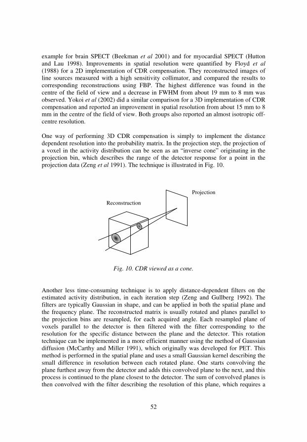
52

example for brain SPECT (Beekman et al 2001) and for myocardial SPECT (Hutton and Lau 1998). Improvements in spatial resolution were quantified by Floyd et al (1988) for a 2D implementation of CDR compensation. They reconstructed images of line sources measured with a high sensitivity collimator, and compared the results to corresponding reconstructions using FBP. The highest difference was found in the centre of the field of view and a decrease in FWHM from about 19 mm to 8 mm was observed. Yokoi et al (2002) did a similar comparison for a 3D implementation of CDR compensation and reported an improvement in spatial resolution from about 15 mm to 8 mm in the centre of the field of view. Both groups also reported an almost isotropic off-centre resolution. One way of performing 3D CDR compensation is simply to implement the distance dependent resolution into the probability matrix. In the projection step, the projection of a voxel in the activity distribution can be seen as an “inverse cone” originating in the projection bin, which describes the range of the detector response for a point in the projection data (Zeng et al 1991). The technique is illustrated in Fig. 10.

Fig. 10. CDR viewed as a cone.

Another less time-consuming technique is to apply distance-dependent filters on the estimated activity distribution, in each iteration step (Zeng and Gullberg 1992). The filters are typically Gaussian in shape, and can be applied in both the spatial plane and the frequency plane. The reconstructed matrix is usually rotated and planes parallel to the projection bins are resampled, for each acquired angle. Each resampled plane of voxels parallel to the detector is then filtered with the filter corresponding to the resolution for the specific distance between the plane and the detector. This rotation technique can be implemented in a more efficient manner using the method of Gaussian diffusion (McCarthy and Miller 1991), which originally was developed for PET. This method is performed in the spatial plane and uses a small Gaussian kernel describing the small difference in resolution between each rotated plane. One starts convolving the plane furthest away from the detector and adds this convolved plane to the next, and this process is continued to the plane closest to the detector. The sum of convolved planes is then convolved with the filter describing the resolution of this plane, which requires a

Projection

Reconstruction

•

53

larger filter kernel. In the backprojection step, the order of this process is reversed (King et al 2004). As for scatter, CDR compensation can however be implemented in the projection step only (Zeng and Gullberg 1992). Compensation for CDR does not only affect the spatial resolution of the reconstructed images. The degradation model implies that more pixels in the projection images will affect the value of a pixel in the reconstructed slice, which will reduce the noise level in the reconstructed images. In theory, it should be possible to recreate the true activity distribution by using compensation for CDR and many iterations (Hutton et al 1997). In practice, however, the increase in noise with successive iterations sets the limit of the image quality that can be achieved. In seems that the inclusion of CDR compensation could affect the choice of collimators to be used for SPECT. Traditionally, high resolution (HR) collimators have been recommended for SPECT (Mueller et al 1986, Madsen et al 1992). However, when using compensation for CDR, Lau et al (2001) demonstrated an increased contrast and recovery of the reconstructions for a general purpose (GP) collimator compared with a HR collimator for myocardial SPECT. Without CDR compensation the HR collimator gave the best results. Their results are interesting and further investigation is needed to see if the conclusions can be applied more generally in SPECT. In Fig. 11, one slice from a reconstruction of a Monte Carlo simulated rCBF study with a noise level that is too low to be clinically realistic, is presented to demonstrate the effect of CDR compensation. The simulated photon energy was 159 keV and the simulated gamma camera was the GE Millennium MG (shown in Fig. 2 d) with LEGP collimators. According to simulations, the system has a spatial resolution of 9.7 mm at a distance of 10.0 cm from the collimator, and the simulated rotation radius was 14.0 cm. The images were simulated without scatter, and were corrected for attenuation. Fig. 11 a shows the true activity distribution in the simulated Zubal phantom for the particular slice, and Fig. 11 b shows one of the simulated 128 projection images to demonstrate the noise level in the projections. Fig. 11 c shows a reconstruction with OSEM using CDR compensation and Fig. 11 d shows the corresponding image reconstructed with FBP using a Hanning low-pass filter (cut-off frequency: 0.90 cm-1) for pre-filtering. The differences in spatial resolution and contrast are apparent. As can be seen, this image also shows that high resolution can be achieved using GP collimators in SPECT, with CDR compensation. It should however be noted that clinical images suffer from a higher noise level than this example, and this impressive image quality is therefore not completely realistic for a clinical case.

54

Fig. 11. rCBF study simulated with 159 keV photons and a LEGP collimator. a: True

activity distribution in the simulated phantom. b: One of the simulated projection

images. c: Reconstruction with CDR compensation. d: Reconstruction with FBP using a

Hanning low-pass filter with 0.90 cm-1

cut-off frequency.

6.3.1 CDR compensation in this work

CDR compensation was included in the iterative reconstructions in the study described in Paper VI. The purpose of this study was to compare three convolution-based techniques and one method implemented in the iterative reconstruction for correction of scatter and septal penetration of 123I brain SPECT. The brain SPECT images were simulated with uptakes corresponding to a DAT study and an rCBF study. Two OSEM programs had to be used for the reconstructions, denoted OSEM-1 and OSEM-2 in the study. The reason was that the method implemented in the iterative reconstruction is connected to OSEM-1 while OSEM-2 had to be used for the images corrected with the convolution-based techniques, since OSEM-2 can reconstruct geometrically mean valued images with attenuation correction. The two OSEM codes showed a clear difference in convergence rate which we had to take into account. Furthermore, the CDR compensations are implemented in different manners in the codes, but it seems that this does not imply any significant differences in image quality. In OSEM-1, a

a b

c d

•

55

rotation-based approach is used, and the resampled planes are filtered in the frequency plane with filters corresponding to the resolution for each distance between the planes and the detector. In OSEM-2, the distance dependence of the point spread function is implemented in the probability matrix. As has been discussed, CDR usually describes the linear increase in the width of the point spread function with increased source-to-collimator distance and this linear model will hereafter be called “linear CDR”. However, this distance dependence cannot be assumed to be true for geometrically mean valued images. The geometrical mean value will reduce the depth dependence of the images, and an option to take this into account was not included in the CDR compensation in the OSEM codes. For simplicity, we therefore implemented a distance-independent correction in OSEM-2, which means that a constant resolution of the system was assumed. This model will hereafter be called “constant CDR”. A constant CDR is of course an approximation, but due to the superior characteristics of CDR compensation compared with other methods to reduce noise and improve resolution, it should be better than to not include the correction. It was of course of interest that the differences between the images reconstructed with compensation for linear CDR and constant CDR should be as small as possible. The choice of constant resolution is not obvious and is likely to depend on activity distribution. We were therefore interested to compare images reconstructed with different resolutions for constant CDR, using OSEM-2, with the same images corrected with linear CDR, using OSEM-1. The comparison was performed for both the DAT and the rCBF simulation included in this study by using the ideal images simulated without the effect of scatter and septal penetration. These images were first reconstructed with linear CDR compensation using OSEM-1 with 8 iterations and 4 projections/subset. Then the geometrical mean values of opposing views of the ideal projection images were calculated and were reconstructed using constant CDR compensation with a range of different resolutions. Due to the difference in convergence rate between the two programs, the number of iterations was varied as well. Optimisation was performed by means of NMSE calculations (see Eq. 25) where the minimum NMSE value was determined. Since both the constant resolutions and the number of iterations were varied, this turned into a 2D optimisation. Attenuation correction was included in all reconstructions using a non-uniform attenuation map calculated from the density map of the brain phantom. After optimisation it was found that a constant resolution of 10.3 mm for the rCBF images and 10.6 mm for the DAT images gave the most similar results compared with the images corrected with linear CDR. For the rCBF images, 24 iterations were required while the DAT images needed 22 iterations to reach approximately the same level of convergence as for 8 iterations with OSEM-1. The resulting images can be seen in Fig. 12 for both studies. A slight difference in resolution can be seen in the peripheral parts of the brain for the rCBF reconstructions, and that should also be expected since the optimal resolution turned out to be the resolution corresponding to a distance of only 2.5 cm from the centre of rotation. Besides from this slight discrepancy the reconstructions show good correspondence.

56

Fig. 12. Images reconstructed with constant CDR (a, b) and linear CDR (c, d).

6.4 Correction for septal penetration Some radionuclides used for scintigraphic imaging emit photons of higher energy than the principal energy used for imaging, for example 123I, 131I and 67Ga. 123I has been used in the studies described in Paper V and VI, and this radionuclide emits high energy photons in less than 3% of the decays, as can be seen in Table I. These photons can however contribute to a significant part of the number of registrations, especially if a collimator optimised for low energies is used (Bolmsjö et al 1977). Such a collimator is effective for absorbing the 159 keV photons with unwanted directions, but it is much less effective of stopping the high energy photons. These photons can penetrate the collimator septa and become registered after scattering in the gamma camera, but they also have a higher probability of becoming registered after scattering in the lead in the collimator. Registrations from collimator scatter will however be included in the term septal penetration in this work. Like scatter, septal penetration registrations will degrade image contrast, and the quantitative accuracy. Artifacts due to septal penetration can also occur. One example is the case with rCBF measurements with N-isopropyl-p-123I-amphetamine (123I-IMP), where the lung uptake is high and septal penetration from lung activity will contribute to the brain images (Macey et al 1986). Septal penetration will

a b

c d

•

57

also make the sensitivity dependent on the distance between the source and the parallel-hole collimator, which affects quantitative accuracy (Fleming et al 1993). Septal penetration will of course decrease if a collimator designed for higher energies, with thicker septa, is used. This will however decrease the spatial resolution, since the hole diameters must be increased to keep the sensitivity. The reduced spatial resolution must then be weighed against the improvements in contrast, the reduced distance dependence of the sensitivity and loss of possible artifacts. There are studies indicating that the use of a medium energy (ME) collimator is preferable to a low energy (LE) collimator for a quantitative evaluation of 123I SPECT (Macey et al 1986, Verberne et al 2005). No ME collimators are however available at the Nuclear Medicine department in Umeå and the total number of examinations that perhaps would benefit from such collimators is small. In Table III, a few parameters of interest are presented for the GP collimators optimised for low energy (LEGP), medium energy (MEGP) and high energy (HEGP) for the Millennium MG used in the study described in Paper VI. The data is picked from a datasheet for the Millennium MG collimator specifications. Table III. Parameters for the GP collimators for the Millennium MG.

Septal thickness

(mm)

Hole diameter

(mm)

Hole length (mm)

Energy (keV) at 5%

penetration

Spatial resolution

(mm) LEGP 0.25 2.5 43 180 10.2 MEGP 1.2 3.0 42 311 12.7 HEGP 1.65 3.4 48 360 13.8

An acquired energy spectrum of a point source of 123I, free in air at a distance of 10 cm from the centre of the Millennium MPR equipped with the LEGP collimator, can be seen in Fig. 13. In this geometry, little of the contribution comes from scatter, and most of the counts outside the photopeak result from septal penetration. It is clear that a significant part of the number of registrations in a photopeak window is due to septal penetration. A number of correction methods for septal penetration have been used, and many methods include this correction in the scatter correction. This may work well for energy window-based correction techniques, but it might not be optimal for correction methods based on modelling the spatial distribution of scatter.

58

Fig. 13. Energy spectra for the Millennium MPR with LEGP collimator.

6.4.1 Energy window techniques

Energy window-based correction methods have been used for correction of scatter and septal penetration in several studies. As has been mentioned, energy window techniques can take contribution from sources outside the field of view into account, which is an advantage. The dual energy window technique has for example been used for correction of 123I brain SPECT on baboons and was found to improve quantitative accuracy (Almeida et al 1999). The TEW method has been used and studied for correction of scatter and septal penetration for 131I and was found to give a reasonable correction (Dewaraja et al 2000). For 123I, Iida et al (1998) improved quantitative accuracy by using TEW for rCBF SPECT with 123I-IMP, but they also reported a clear increase in noise level. Inoue et al (2004) and Verberne et al (2005) used TEW for relative quantification of myocardial SPECT studies performed with 123I-meta-iodobenzylguanidine (123I-MIBG). In both studies the image contrast was improved, but the use of TEW provided little extra information and the choice of collimator was concluded to be more important. Pollard et al (1996) evaluated five window-based techniques for 131I and compared them with a spectrum-fitting method which is based on fitting the observed energy spectrum to a function modelling scatter (including septal penetration) and the photopeak. It was found that all window-based methods performed better than to use no correction, but they concluded that the spectrum-fitting approach was the most promising technique. It should be noted energy window techniques are not as effective for correction of septal penetration of photons with the principal energy used for imaging. Since these photons have the same energy as the geometrically collimated photons, it is not possible to discriminate these photons from one another in the energy spectrum (Dewaraja et al 2000).

Point source of 123I, 10 cm distance

0

5000

10000

15000

20000

25000

30000

0 100 200 300 400 500 600

Energy (keV)

•

59

6.4.2 Convolution techniques

Convolution and deconvolution have also been used to correct for septal penetration. Fleming et al (1993) used CSS for quantification of 131I SPECT which included a monoexponential or a biexponential kernel to model scatter and septal penetration combined. Fleming and Alaamer (1996) did a further investigation and compared the spatial spread of 131I registrations from a line source with corresponding measurements using 99mTc and 123I. The comparison with 99mTc clearly demonstrated that the spatial spread of registrations from septal penetration is wider compared with registrations from scatter. Deconvolution has for example been used by Shen et al (1994) and Sjögreen et al (2002). They used inverse filtering with a Wiener filter to correct for scatter and septal penetration in 90Y and 131I planar imaging, respectively. TDCS has been modified to take septal penetration into account by a constant added to the matrix of scatter fractions, k0 (Iida et al 1998). The following equation is then used for calculating the scatter fractions, for one TDCS iteration:

02/),(),( k

yxtA

11 yxk +

−−=

βα (28)

The same kernel is used to correct both for scatter and septal penetration, which is an approximation because of the difference in spatial distribution. When TDCS was compared with TEW for rCBF SPECT using 123I, no significant difference was found, except for the previously mentioned increased noise level for the TEW-corrected images (Iida et al 1998). The higher noise level reported for the TEW method is this study has however been questioned (Zaidi and Koral 2004). 6.4.3 Septal penetration in an iterative reconstruction procedure

Correction for septal penetration has also been implemented in the iterative reconstruction by including the penetration component in the CDR correction (Ljungberg et al 2002, He et al 2005). The method is based on a table of response functions including septal penetration, generated as a function of the distance from the collimator by using Monte Carlo simulations of point sources in air. The shape of each response function is dependent on the distance from the collimator, but it is spatially invariant for a certain distance. The response functions are normalised so that the total sum of each function equals the total to primary ratio for that specific distance. The correction is implemented in the projection step in OSEM using the rotation-based approach described previously. For each projection angle, the estimated 3D activity distribution is resampled to planes parallel to the detector. Each plane is then filtered in the frequency plane, with the corresponding response function including septal penetration, for that distance.

60

6.4.4 Correction for septal penetration in this work

In the study described in Paper VI, correction for scatter and septal penetration was evaluated for brain SPECT using 123I-labelled compounds. The Monte Carlo program described in Paper V was used for simulation of the brain SPECT images. As has been mentioned, the purpose of this study was to compare three convolution-based techniques, which subtract scatter and septal penetration registrations from the projection images, with a method included in the iterative reconstruction. The convolution-based methods were CSS, TDCS as described in Eq. 28 and a modified TDCS version proposed by us. The method included in the iterative reconstruction uses ESSE to model scatter and CDR compensation including septal penetration, as described above. The corrections were evaluated for two brain SPECT activity distributions, one corresponding to a DAT study and one corresponding to an rCBF study. The Zubal phantom was used for simulations of these studies, and images including registrations from scatter and septal penetration were simulated together with ideal images without these registrations. rCBF studies are seldom performed with 123I labelled compounds today since 99mTc-labelled compounds are less expensive and have favourable dosimetry. The previously mentioned 123I-IMP seems still to be in use, however. The reason for including the rCBF simulation in this study is that its activity distribution is more complex compared with the DAT study, and that should imply clearer differences between the correction methods. The new TDCS version proposed in Paper VI uses a separate kernel to correct for the registrations from septal penetration. This is an attempt to improve the method described in Eq. 28 since that method uses the same kernel to model both scatter and septal penetration. This implies that the method has to be divided into two steps, one CSS step to correct for septal penetration, and one TDCS step to correct for the scattered registrations. The equation for the image corrected for septal penetration, gsp(x,y), will then be:

)),((),(),( spobsspobssp syxgkyxgyxg ⊗−= (29)

where ksp is the penetration-to-total ratio and ssp is a monoexponential kernel describing the septal penetration registrations. Eq. 23 and Eq. 24 were then used for scatter correction of gsp(x,y). The optimisation of kernels and geometries to derive the scatter fractions were performed in a likewise manner as described in Paper III for all three 2D correction methods. The optimisation for the new TDCS version was however rather time-consuming since the scatter and penetration kernels had to be varied independently and a 2D kernel optimisation was required for each geometry to derive scatter fractions. The comparison of the different correction methods was not straightforward since two different OSEM codes had to be used, OSEM-1 and OSEM-2, and the reason for this has been described in a previous section. The ESSE and CDR correction with the penetration component was connected to OSEM-1, while OSEM-2 had to be used for

•

61

reconstruction of the geometrically mean valued images, using the constant CDR compensation. It was however possible to obtain reconstructions with similar quality from these two codes with the different methods for CDR compensation, as can be seen in Fig. 12. Attenuation correction was included in all reconstructions using a non-uniform attenuation map calculated from the density map of the Zubal phantom. The evaluations of the different correction methods were carried out by means of NMSE calculations (see Eq. 25) of all pixels within the brain. Two different comparisons were performed. All images corrected for scatter and septal penetration were compared with the ideal images reconstructed using linear CDR with OSEM-1. This calculation gives the overall error when comparing to the ideal image with the best image quality. The CSS- and TDCS-corrected images were also compared with a reconstruction of the geometrically mean valued ideal images with constant CDR compensation using OSEM-2. In this comparison the differences originating from the constant CDR correction are cancelled out and this comparison gives the errors from the limitations in the corrections. The contrast improvement for all corrections was also evaluated. For the DAT images the ratio of counts in the striatum structures compared with the rest of the brain was calculated, while the ratio of grey-to-white matter counts was calculated for the rCBF images. The results in Paper VI show that the method included in the iterative reconstruction provides the most accurate results and that our new TDCS version gives better results compared with the other 2D methods. All methods in the study improve however the quantitative accuracy compared to when the corrections are not included. This study also shows that all corrections improve image contrast, to a great extent.

62

7 CORRECTIONS FOR PLANAR SCINTIGRAPHIC IMAGING

In contrast to SPECT, the whole patient can be examined when using planar scintigraphic imaging, by the whole-body scanning available on modern equipment. This can for example be an advantage for oncology purposes. The images reflect however a 2D projection of the 3D activity distribution and the activity in the different tissues will therefore be superimposed, as seen on the images. This is a complicating factor for both absolute and relative quantification. In absence of background activity and overlapping structures, the uncertainty in quantitative accuracy can be as low as 10% (King and Farncombe 2003). Attenuation and contribution from background activity are two factors that need to be corrected for in planar scintigraphic imaging, for a reasonable accurate quantification. Scatter can also be compensated for, and correction for septal penetration may be needed for some radionuclides. Techniques for correction of scatter and septal penetration in SPECT have been presented and some of them are also applicable to planar imaging, for example techniques based on measurements in separate energy windows. Convolution techniques can be used for a conjugate view setting. Other techniques that can be used for scatter correction of planar images are presented in MIRD Pamphlet no. 16 (Siegel et al 1999). If scatter correction is not used, which is often the case, an experimentally determined effective attenuation coefficient should be used for attenuation correction since the loss of counts otherwise will be over-compensated. 7.1 Attenuation correction For attenuation correction of planar scintigraphic images, it can be an advantage to use the conjugate view technique, that is to calculate the geometrical mean value of opposing views (Sorenson 1971, Thomas et al 1976). The calculation of geometrical mean values for attenuation correction has already been discussed in this work in the section about attenuation correction in SPECT. In most cases an anterior and posterior view of the patient is used for this purpose, but the technique is applicable for any image pair, separated 180°. The geometrical mean value will reduce the need for exact depth information of the source within the body, but scatter free images are required for complete removal of depth dependence (King and Farncombe 2003). The conjugate view technique is sometimes used clinically for cancelling the effect of attenuation when relative quantification is of interest, for example in gastric emptying (Ziessman et

al 2004). The rest of this section will however deal with absolute quantification, since correction techniques seldom are applied for a relative quantification or visual interpretation of planar images. Many analytical functions have been presented for absolute quantification based on the conjugate view technique, with different complexity of the source and attenuation geometry. One must however remember that they are more or less severe approximations of the complex geometry within the patient. Fleming (1979) developed an equation for attenuation correction for a rod of activity, where the rod and the

•

63

surrounding tissue have different attenuation coefficients. Other configurations that can be of interest are presented by Thomas et al (1976). One of these geometries is shown in Fig. 14. It is based on a single uniform source in a medium consisting of n regions with different attenuation coefficients (Thomas et al 1976, Siegel et al 1999). The activity in the source, Aj, can be calculated as:

C

f

T

RRA

j

e

PA

j )exp( µ−= (30)

where RA and RP are the anterior and posterior count rate, respectively, and C is the sensitivity. µe is the total weighted linear attenuation coefficient, which can be calculated as:

∑ ==

n

i iie tT 1

1µµ (31)

and fj accounts for the attenuation and thickness of the source region:

)2/sinh(

)2/(

jj

jj

jt

tf

µ

µ= (32)

Fig. 14. Geometry for a single uniform source.

It should be noted that the above equations assumes images free from scatter (Siegel et

al 1999). It has been shown that accurate values of attenuation coefficients and patient

µn

t1

tj

tn

T µj

RP

RA

Posterior

Anterior

µ1

64

thicknesses are very important for the activity estimate, using the conjugate view technique (Norrgren et al 2003). It is therefore advantageous to use a 2D attenuation map for attenuation correction. 2D attenuation maps accounts for the factor exp(-µeT) in Eq. 30 and can be determined from transmission measurements (Graham and Neil 1974, Myers et al 1981, Delpon et al 2002), CT images (Liu et al 1996, Miller et al 1996, Skretting et al 1997) or both (Sjögreen et al 2002). Transmission measurements in scintigraphic imaging have been discussed for SPECT, but can also be used for scintigraphic imaging with a stationary gamma camera. Geometries with a planar source (Graham and Neil 1974, Myers et al 1981) or a scanning line source (Delpon et al 2002) have been used together with parallel-hole collimators. In the 2D case the transmission factors, exp(-µeT), can be determined by a pixel-by-pixel division of a transmission measurement with the patient present and a corresponding measurement without the patient present. If the transmission and emission radionuclides are different, the transmission factors must be scaled to match the emission attenuation coefficients. The transmission factors can then be used for input in Eq. 30. Attenuation maps determined from CT images have also been described previously. CT images give however information on attenuation in 3D, and this information have been used in different ways to correct for attenuation in the 2D planar scintigraphic images (Liu et al 1996, Miller et al 1996, Skretting et al 1997, Sjögreen et al 2002). If only one scintigraphic image is measured, a simplified method assuming an effective point source can be used (Siegel et al 1999). The method assumes that the depth distribution of the activity is concentrated into a point source of equal activity at an effective depth within the patient (Jones and Brill 1975). This source depth is then used for attenuation correction. The depth can be determined from a lateral view of the patient (Siegel et al 1999) or perhaps from a 3D image volume acquired by another modality, for example CT or MRT images. This type of measurement can be better than a conjugate view approach if the source contrast is poor in one of the views, which for example can be the case for small superficial sources (Shen et al 1994). If we assume an anterior view, the activity A can be calculated from:

C

dRA dA )exp(µ

= (33)

where d is the effective source depth, and µd is the weighted attenuation coefficient from the source in the anterior direction (Siegel et al 1999). If the effective point source method is a too rough approximation, which can be the case for thick sources (Jones and Brill 1975), an integration over the source thickness must be performed, for attenuation correction.

•

65

7.2 Background correction In most practical cases, over- and underlying activity will contribute to the counts in the ROI used for quantification. The background counts can for example originate from activity circulating in the blood or activity distributed in other tissues. A correction for this background is usually needed, in combination with attenuation correction, for an accurate quantification. Otherwise the calculated activity in the source will be overestimated. Background correction can be a complex issue, depending on the complexity of the activity distribution in different tissues in the body. A background ROI is typically used, where the geometry and uptake should be as close to the source ROI as possible, except for the source uptake to be quantified. This ROI can for example be placed close to the source ROI or contralateral on the patient. Straightforward subtraction of the counts of this background ROI would however lead to an underestimation of the source activity unless the volume of the source can be neglected. The reason is that the counts from the volume in the background ROI corresponding to the source should not be included in the subtraction (Kojima et al 1993). For a simple conjugate view geometry with a single uniform source, like in Fig. 14, and a homogeneous background activity outside of the source, a simple correction technique can be applied. Assume a background ROI of the same size beside the source ROI in Fig. 14, and that the count rate from the geometrical mean value of this ROI is RB. The fraction of counts originating from the source can then be calculated as (Siegel et al 1999):

2/1)])1(1)][1(1([T

t

R

R

T

t

R

RF

j

P

Bj

A

B −−−−= (34)

In Eq. 30, (RARP)1/2 should then be replaced by F(RARP)1/2 when calculating the source activity. For a single view setting, a method by Kojima et al (1993) has been shown to be relatively accurate (Buijs et al 1998). In this case a background corrected value of the anterior countrate is calculated as:

BCBAcorr RRRR +−= (35) where RBC is the background count rate from the from the volume equivalent to the source. This term is calculated as (Kojima et al 1993):

)exp(1

)exp(1)exp(

T

tdRR

d

jd

dBBCµ

µµ

−−

−−−= (36)

using the same notations as in Fig. 14.

66

7.3 Attenuation and background correction in this work In the study described in Paper I, a method for estimating the activity in a tumour inoculated subcutaneously in the flank of a mouse, was developed. The setup of the equipment can be seen in Fig. 15, where a sleeping mouse is positioned on a holder connected to the pin-hole collimator. It should however be mentioned that the pin-hole collimator in this image does not belong to the Porta Camera used in this study, but another analogue camera which also has been used for mouse studies. A single view was acquired for each “whole-body” mouse examination, since a conjugate view setup was not an issue with the Porta Camera, which needs manual control of position. From the activity estimation the dose to the tumour could be calculated.

Fig. 15. Measurement geometry for mouse studies.

The geometry with the tumour on the side of the mouse is a special case, compared with the general equations presented. The tumour protrudes, and therefore a part of the tumour is covered only with skin, which contributes little to background activity. The other side of the tumour represses normal tissue, which contributes more to the background activity. An equation for the photon escape probability from the tumour was determined for attenuation correction. It was calculated using Taylor series expansion, assuming that

•

67

the tumour was a spherical object. This probability was expressed as a function of tumour mass m as:

3/23/1

4

3

5

2

4

3

4

31

+

−≈

πρµ

πρµ

mmNesc (37)

where µ is the attenuation coefficient in the tumour and ρ is the corresponding density that was assumed to be 1.0 g/cm3. The tumour mass was determined by volume measurements with a calliper. A subtraction of the background counts in the tumour ROI was needed, and two different ROI setting techniques for background subtraction were evaluated. One of the methods was based on two rectangular ROIs, one over the tumour and one background ROI on the contralateral side. The background ROI was positioned at the same distance from the median line of the mouse as the tumour ROI. For the other ROI setting irregular ROIs were used, with a background ROI surrounding the tumour ROI. The tumour and background ROI settings can be seen in Fig. 16. A ROI covering the whole mouse was also set on all images.

Fig. 16. Tumour and background ROI setting.

A simple mass-dependent background correction was performed with the following equation:

B

TBBTnet

M

MMCCC

−−= (38)

68

Cnet are the net counts from the tumour, CT are the counts in the tumour ROI, CB are the counts in the background ROI (with the same area as the tumour ROI), MT is the tumour mass and MB is the mass of the normal tissue in the background ROI. The latter was calculated as the fraction of counts in the background ROI to the whole mouse ROI, times the mass of the mouse. The activity in the tumour was finally calculated as:

tN

KCA

esc

net

T = (39)

where K is a geometry dependent constant, determined from calibrations, and t is measurement time. The calculated activities were compared with the tumour activities measured in vitro, and it was found that the contralateral ROI setting gave the best result. The (measured in vivo)/(measured in vitro) activity ratios were 1.04 for the contralateral ROI setting and 0.77 for the ROI setting with the larger background ROI. The corresponding standard deviations were 17% and 24%, respectively.

•

69

8 SUMMARY AND CONCLUSIONS

8.1 Paper I A method was evaluated for estimating the activity of 125I in a tumour inoculated in the flank of a mouse, with a gamma camera equipped with a pin-hole collimator. Two different methods of background subtraction were compared, one with a contralateral ROI setting and one with a larger background ROI surrounding the tumour ROI. The method using the contralateral ROI-setting gave the most accurate results. The poor results of the other technique can be explained by scattered photons from the tumour in the background ROI and that this background ROI comes closer to the centre of the mouse where the activity is higher. The high standard deviations of the (measured in

vivo)/(measured in vitro) activity ratios are likely to depend mostly on the measurement geometry with the pin-hole collimator. Exact position on the tumour in the reference point is essential since sensitivity is dependent on the distance from the pin-hole. Other uncertainties are the accuracy of the measurements in vitro, differences in tumour activity between the in vivo and in vitro measurements and uncertainties in tumour mass. The method can be useful for studies of radioimmunotargeting of tumours with labelled antibodies when determining the average value of tumour uptake in a group of mice.

8.2 Paper II A method for attenuation and scatter correction of brain SPECT based on CT images was developed, where the CT images were used as bases for calculation of attenuation maps. The attenuation maps were used both for attenuation correction and for deriving scatter fractions for the TDCS scatter correction method. A method for registering of the CT and SPECT image volume using fiducial markers that only needed to be present during the SPECT study was investigated. The rationale for this is that the CT scan is usually performed before the SPECT scan in clinical practice at Norrlands University Hospital, and it is not known in advance if a patient will undergo both examinations. When pointing out the landmarks in the CT image volume, the distances between the markers, known from the SPECT images, were taken into account. With the current simple Matlab-based software, it was found that the uncertainty of the method is a little too high for the method to be used for individual quantification for rCBF studies. A more advanced user interface would probably improve the accuracy, however. The method should be most useful for examinations with radiopharmaceuticals with low uptake in the peripheral parts of the brain, for example DAT studies, since the errors due to mismatching were low in central structures. In these types of studies it is also difficult to find the head contour in the SPECT images, which makes the estimation of a uniform attenuation map difficult. 8.3 Paper III In this study, TDCS was optimised for scatter correction of 99mTc HMPAO rCBF SPECT. The most optimal of four geometries to derive scatter fractions as a function of attenuation path length, and the optimal scatter kernel, were determined. CSS is also

70

evaluated in this study, and in this case a constant scatter fraction corresponding to each geometry was tested for comparison. All corrected image volumes were compared with the ideal image volume simulated without scatter, by means of the NMSE of normalised images. The normalisation step was included since the images are intended for relative quantification. For TDCS it was found that the best of the four tested geometries was a slab of homogeneous activity distribution. However, this geometry underestimates scatter in the brain, and would probably not be optimal for a NMSE calculation without normalisation. For CSS the optimal scatter fraction was close to the scatter-to-total ratio for the phantom simulation. The optimal scatter kernel slope for CSS was steeper than the corresponding slope for TDCS, because of the curvature effect introduced when multiplying the convolved images by the matrix of scatter fractions used by TDCS. It was found that both TDCS and CSS provide superior accuracy when compared to when scatter correction is omitted. TDCS can however give better results than CSS if used with optimal parameters, and one can expect that the differences between the methods will increase for tissues with less homogeneous density distributions. 8.4 Paper IV

TDCS has been claimed to be an iterative technique. An iterative approach requires however a modification of the existing theory on how to calculate the scatter fractions. For one TDCS iteration, the matrix of scatter fractions is based on the scatter-to-total ratio. This should however not be the case for several iterations, since an already scatter corrected image consists mostly of primary photons. The matrix of scatter fractions should therefore be based on scatter-to-primary ratios, after the first iteration. To prove this, a point-source in a water phantom was simulated and the image was scatter corrected using TDCS based on iterative and non-iterative approaches. The ratios of subtracted to original counts were then compared with the scatter-to-total ratio known from the simulation, and it was found that scatter-to-primary ratios should be used for iterative TDCS after the first iteration. The iterative method is theoretically appealing but it is not certain if it will improve the scatter estimate in practical cases, and this requires further investigation. The iterative method is however significantly slower since the convolution step in TDCS has to be performed several times. 8.5 Paper V A new version of the Monte Carlo program SIMIND is evaluated in this study. The new code can take collimator interactions in a hexagonal hole collimator into account, using the Delta-Scattering technique. Collimator interactions are important when studying radionuclides emitting high energy photons, such as 123I, 131I, and 67Ga, since septal penetration and collimator scattering are significant for these radionuclides. The evaluation was performed using a gamma camera with wide scatter free surroundings, equipped with either a LEGP or a LEHR collimator. For the evaluation, simulated and measured images and energy spectra of point sources and a striatal phantom were compared. A good correspondence was found. There are however some differences which for example can depend on differences between the collimator geometry specifications and the true geometry. Other minor differences resulting from inexact

•

71

matching of the Monte Carlo model and the gamma camera system are of course also present. 8.6 Paper VI In this study four different correction methods for scatter and septal penetration are evaluated for 123I brain SPECT, using the Monte Carlo program described in the previous study. The corrections are CSS, two TDCS versions, one of them proposed by us, and a method where the corrections are included in the iterative reconstruction. The latter method uses ESSE to correct for scatter and CDR compensation including both geometric and penetration components. The new TDCS version separates the correction for scatter and septal penetration in one CSS step that corrects for septal penetration with a “penetration kernel” and one TDCS step to correct for scatter. The methods were evaluated for two types of studies, a DAT study and an rCBF study performed with 123I. To get an approximately equivalent image quality for all OSEM reconstructions, CDR compensation was included also for the images corrected using CSS and TDCS. These corrections operate on geometrically mean valued images, and a distance-independent CDR correction was therefore applied. The methods were evaluated in terms of quantitative accuracy and contrast improvement. It was found that all correction methods included in this study improve image contrast. For quantitative accuracy, this study shows that the method included in the iterative reconstruction provides the most accurate results and that our new TDCS version gives higher accuracy compared with the other 2D methods. It is clear that quantitative accuracy in brain SPECT benefits from separate modelling of scatter and septal penetration.

72

9 FUTURE PERSPECTIVES The importance of using corrections for improving the quantitative accuracy of SPECT and planar scintigraphic imaging is well known. Absolute quantification of activity is important for therapeutic purposes, while relative quantification has more applications in diagnostics. Corrections are also beneficial for a visual interpretation of the images in many cases. Attenuation correction has traditionally been performed with simplified models assuming uniform attenuation in the patient. This can however be a too rough approximation, especially for imaging of the heart and lung region. Commercial equipment with transmission sources have existed for a number of years, and with accurate quality control they can provide valuable information. In recent years SPECT/CT hybrid systems have been developed where the CT images can be used for calculation of attenuation maps, but they also provide accurate anatomical information for the functional data. These systems are likely to be more common in the future since the increased use of multimodality systems is a general trend in diagnostics. With increased use of non-uniform attenuation correction, the popularity of iterative reconstruction procedures like OSEM will probably increase and this can simplify the introduction of other corrections. On modern gamma camera systems the capability of measuring in more than one energy window is wide-spread. This makes it possible to implement different window-based correction techniques for scatter and septal penetration. If a non-uniform attenuation map is used for attenuation correction, the TDCS method evaluated in this work can be an alternative. The implementation of scatter correction into clinical practice has however been rather slow so far, and a reason for this is probably the increased noise level when the scatter estimates are subtracted. A fast and accurate method that can be included in the iterative reconstruction is probably needed for scatter corrections to be more widely applied. Compensation for CDR can improve spatial resolution and decrease the noise level when included in the iterative reconstruction. CDR compensations have been integrated in the reconstruction software of some manufacturers of gamma camera systems, and this technique is likely to be more common in the future. The increase in computing time when including all corrections in the iterative reconstruction must however be taken into account. With the filtered back projection technique, the reconstruction times have been very short, and the popularity of these techniques will depend on the acceptance of the clinicians to wait for the reconstructions. Changes in clinical routines and perhaps special reconstruction computers may be needed for the cases where image quality and/or accurate quantification are of high priority.

•

73

10 ACKNOWLEDGEMENTS I would like to express my warm and sincere gratitude to: My supervisor Lennart Johansson. I have had a great time these years and I can’t thank you enough, but thanks anyway for all help, stimulating discussions and for the time you have dedicated to my work. My supervisor Katrine Åhlström Riklund for believing in me from the start and for sharing some of your knowledge in radiology. Michael Ljungberg for introducing me to SIMIND, for all help with the Monte Carlo simulations and for the collaboration on the last two papers. What would I have done without you? My friend and coworker Torbjörn Sundström for support, encouragement and for sharing your inspiring ideas with me. Mikael Karlsson for being my examiner and for support and valuable advice. Anna Wernblom for excellent help with administrative issues. Hans Svensson and Sven-Ola Hietala for support during my first years as a PhD student. Susanna Jakobson Mo for collaboration with the design of the digital DAT-phantom. The staff at the Nuclear Medicine department for providing me with radionuclides, for assistance with the marker settings in Paper II and for trusting me with your equipment. Lars Nyberg, the rest of the fMRI group and the staff at the MR-department for providing me with interesting work outside the world of SPECT corrections and for being supportive and understanding, especially during the last months of writing. Eva Elgh for collaboration in other studies and for trying to cool me down during stressful times. Richard Larkin for valuable help with OSEM. Stig Larsson and Cathrine Jonsson for a two-week introduction to the field a number of years ago. Thord Holmström for the small and clever holders for the radioactive markers. Anders Hellenäs, GE Healthcare, for letting us play with the striatal phantom for research purposes.

74

Birgitta Lanhede for support and for patiently waiting for me to get finished. The rest of the staff at the Radiation Physics department for being nice colleagues. Special thanks to my PhD student colleagues during the years, and to the diagnostic engineers for all help! My mother, father and brother with family for continuous support and for showing interest in my work. My friends for just being. How on earth do you put up with me? And last but certainly not least to Björn for love, support and tolerance.

This work has been supported by grants from Lion’s Cancer Research Foundation in Northern Sweden, the Swedish Knowledge Foundation and the Faculty of Medicine, Umeå University.

•

75

11 REFERENCES Almeida P, Ribeiro MJ, Bottlaender M, Loc'h C, Langer O, Strul D, Hugonnard P, Grangeat P, Maziere B, Bendriem B. Absolute quantitation of iodine-123 epidepride kinetics using single-photon emission tomography: comparison with carbon-11 epidepride and positron emission tomography. Eur J Nucl Med 1999 26: 1580-1588 Andersen AR. 99mTc-D,L-hexamethylene-propyleneamine oxime (99mTc-HMPAO): basic kinetic studies of a tracer of cerebral blood flow. Cerebrovasc Brain Metab Rev 1989 1: 288-318 Anderson DW. Absorption of ionizing radiation. University Park Press, Baltimore 1984 Andreo P. Monte Carlo techniques in medical radiation physics. Phys Med Biol 1991 36: 861-920 Anger HO. Scintillation camera, Rev Sci Instr 1958 29: 27-33 Anger HO. Scintillation camera with multichannel collimators. J Nucl Med 1964 5: 515-531 Attix FH. Introduction to radiological physics and radiation dosimetry. John Wiley & Sons, Inc. New York 1986 Axelsson B, Israelsson A, Larsson S. Non-uniformity induced artefacts in single-photon emission computed tomography. Acta Radiol Oncol 1983 22: 215-224 Axelsson B, Msaki P, Israelsson A. Subtraction of compton-scattered photons in single-photon emission computed tomography. J Nucl Med 1984 25: 490-494 Bailey DL. Transmission scanning in emission tomography. Eur J Nucl Med 1998 25: 774-787 Beekman FJ, Kamphuis C, King MA, van Rijk PP, Viergever MA. Improvement of image resolution and quantitative accuracy in clinical single photon emission computed tomography. Comput Med Imaging Graph 2001 25: 135-146 Beekman F. J , W.A.M de Jong H, van Geloven S. Efficient fully 3-D iterative SPECT reconstruction with Monte Carlo-based scatter compensation. IEEE Trans Med Imaging 2002 21: 867-877 Binkley D, Young J. An electronic detector simulator for testing position, energy, and timing spectral performance of detector electronics. IEEE Trans Nucl Sci 1998 45: 782-786

76

Blankespoor SC Wu X, Kalki K, Brown JK, Cann CE, Hasegawa BH. Attenuation correction of SPECT using X-ray CT on an emission-transmission CT system: Myocardial perfusion assessment. IEEE Nuclear Science Symposium and Medical

Imaging Conference Record 1995 2: 1126-1130 Bolmsjö MS, Persson BRR, Strand SE. Imaging 123I with a scintillation camera. A study of detection performance and quality factor concepts. Phys Med Biol 1977 22: 266-277 Booij J, Tissingh G, Winogrodzka A, Boer GJ, Stoof JC, Wolters EC, van Royen EA, Practical benefit of [123I]FP-CIT SPET in the demonstration of the dopaminergic deficit in Parkinson's disease. Eur J Nucl Med 1997 24: 68-71 Briesmeister JF. A general Monte Carlo code for neutron and photon transport. Los

Alamos Scientific Laboratory Technical Report LA-7396-M 1986 Browne J and De Pierro A, A row-action alternative to the EM algorithm for maximizing likelihoods in emission tomography, IEEE Trans Med Imaging 1996 15: 687-699 Buijs WCAM, Siegel JA, Boerman OC, Corstens FHM. Absolute organ activity estimated by five different methods of background correction. J Nucl Med 1998 32: 2167-2172 Buvat I, Benali H, Todd-Pokropek A, Di Paola R. Scatter correction in scintigraphy: the state of the art. Eur J Nucl Med 1994 21: 675-694 Buvat I, Castiglioni I. Monte Carlo simulations in SPET and PET, Q J Nucl Med 2002 46: 48-61 Byrne CL. Block-iterative methods for image reconstruction from projections. IEEE

Trans Image Processing 1996 5: 792-793 Celler A, Sitek A, Stoub E, Hawman P, Harrop R, Lyster D. Multiple line source array for SPECT transmission scans: simulation, phantom and patient studies. J Nucl Med 1998 39: 2183-2189 Celler A, Dixon KL, Chang Z, Blinder S, Powe J, Harrop R. Problems created in attenuation-corrected SPECT images by artifacts in attenuation maps: a simulation study. J Nucl Med 2005 46: 335-343 Chang LT. A method for attenuation correction in radionuclide computed tomography. IEEE Trans Nucl Sci 1978 25: 638-643 Chornoboy ES, Chen CJ, Miller MI, Miller TR, Snyder DL. An evaluation of maximum likelihood reconstruction for SPECT. IEEE Trans Med Imaging 1990 9: 99-110

•

77

Cormack AM. Representation of a function by its line integrals with some radiological applications. J Appl Phys 1963 34: 2722-2727 Curry, III TS, Dowdey JE, Murry, Jr RC. Christensen’s Physics of Diagnostic Radiology. Lea & Febiger Philadelphia 1990 de Vries DJ, Moore SC, Zimmerman RE, Mueller SP, Friedland B, Lanza RC. Development and validation of a Monte Carlo simulation of photon transport in an Anger camera. IEEE Trans Med Imaging 1990 9: 430-438 de Vries DJ, Moore SC. Monte Carlo simulation of photon transport in gamma camera collimators. In: Ljungberg M, Strand SE, King MA editors. Monte Carlo calculations in nuclear medicine. Bristol and Philadelphia: IOP Publishing Ltd 1998 Delpon G, Ferrer L, Lenta C, Lisbona A, Buvat I, Bardiès M. Comparison of four scatter correction methods for patient whole-body imaging during therapeutic trials with Iodine-131. Cancer 2002 94: 1224-1230 Devous MD, Stokely EM, Chehabi HH, Bonte FJ. Normal distribution of regional cerebral blood flow measured by dynamic single-photon emission tomography. J Cereb

Blood Flow Metab 1986 6: 95-104 Dewaraja YK, Ljungberg M and Koral KF. Characterization of scatter and penetration using Monte Carlo simulation in 131I imaging. J Nucl Med 2000 41: 123-130 Ficaro EP, Fessler JA, Shreve PD, Kritzman JN, Rose PA, Corbett JR. Simultaneous transmission/emission myocardial perfusion tomography. Diagnostic accuracy of attenuation-corrected 99mTc-sestamibi single-photon emission computed tomography. Circ 1996 93: 463-73 Fleming JS. A technique for the absolute measurement of activity using a gamma camera and computer. Phys Med Biol 1979 24: 176-180 Fleming JS. A technique for using CT images in attenuation correction and quantification in SPECT. Nucl Med Commun 1989 10: 83-97 Fleming JS, Alaamer AA, Perring S. A technique for the absolute quantification of 131I radiopharmaceuticals using SPECT. Nucl Med Commun 1993 14: 498-505 Fleming JS, Alaamer AS. Influence of collimator characteristics on quantification in SPECT. J Nucl Med 1996 37: 1832-1836 Floyd CE, Jaszczak RJ, Greer KL, Coleman RE. Deconvolution of Compton scatter in SPECT. J Nucl Med 1985 26: 403-408

78

Floyd CE, Jaszczak RJ, Greer KL, Coleman RE. Inverse Monte Carlo as a unified reconstruction algorithm for ECT. J Nucl Med 1986 27: 1577-1585 Floyd CE, Jaszczak RJ, Coleman RE. Convergence of the maximum likelihood reconstruction algorithm for emission computed tomography. Phys Med Biol 1987 32: 463-476 Floyd CE, Jaszczak RJ, Manglos SH, Coleman RE. Compensation for collimator divergence in SPECT using inverse Monte Carlo reconstruction. IEEE Trans Nucl Sci 1988 35: 784-787 Frey EC, Tsui BMW, Ljungberg M. A comparison of scatter compensation methods in SPECT: Subtraction-based techniques versus iterative reconstruction with accurate modeling of the scatter response. Conference Record of the 1992 Nuclear Science

Symposium and the Medical Imaging Conference 1992 1035-1037 Frey EC, Tsui BMW. A practical method for incorporating scatter in a projector-backprojector for accurate scatter compensation in SPECT. IEEE Trans Nucl Sci 1993 40: 1107-1116 Frey EC, Tsui BMW. A new method for modelling the spatially-variant, object-dependent scatter response function in SPECT. IEEE Nuclear Science Symposium 1996. Conference Record 2: 1082-1086 Gilbert P. Iterative methods for the tree-dimensional reconstruction of an object from projections. J Theor Biol 1972 36: 105-117 Gillen GJ. A simple method for the measurement of local statistical noise levels in SPECT. Phys Med Biol 1992 37: 1573-1579 Gindi G, Lee M, Rangarajan A, Zubal IG. Bayesian reconstruction of functional images using anatomical information as priors. IEEE Trans Med Imaging 1993 12: 670-680 Goitein M. Three-dimensional density reconstruction from a series of two-dimensional projections. Nucl Instrum Meth 1972 101: 509-518 Gordon R, Bender R, Herman GT. Algebraic reconstruction techniques (ART) for three-dimensional electron microscopy and x-ray photography. J Theor Biol 1970 29: 471-481 Graham LS, Neil R. In vivo quantitation of radioactivity using the Anger camera. Radiology 1974 112: 441-442 Gullberg GT, Huesman RH, Malko JA, Pelc NJ, Budinger TF. An attenuated projector-backprojector for iterative SPECT reconstruction. Phys Med Biol 1985 30: 799-816

•

79

Hamilton DI. Diagnostic Nuclear Medicine A Physics Perspective. Springer Verlag Berlin 2004 Harrison RL, Vannoy SD, Haynor DR, Gillipsie SB, Kaplan MS, Lewellen TK. Preliminary experience with the photon history generator module of a public domain simulation system for emission tomography. Proceedings of the IEEE Nuclear Science

Symposium and Medical Imaging Conference 1993 1154-1158 Hart GC. Quality assurance of gamma cameras and computers. In: Hart GC and Smith AH editors. Quality standards in nuclear medicine. The Institute of Physical Sciences in Medicine 1992 York Hashimoto J, Sasaki T, Ogawa K, Kubo A, Motomura N, Ichihara T, Amano T, Fukuuchi Y. Effects of scatter and attenuation correction on quantitative analysis of beta-CIT brain SPET. Nucl Med Commun 1999 20: 159-165 Haynor DR. Variance reduction techniques. In: Ljungberg M, Strand SE, King MA editors. Monte Carlo calculations in nuclear medicine. Bristol and Philadelphia: IOP Publishing Ltd 1998 He B, Du Y, Song X, Segars WP, Frey EC. A Monte Carlo and physical phantom evaluation of quantitative In-111 SPECT. Phys Med Biol 2005 50: 4169-4185 Herbert T, Leahy R. A generalized EM algorithm for 3-D Bayesian reconstruction from Poisson data using Gibbs priors. IEEE Trans Med Imaging 1989 8: 194-202 Hounsfield GN. Computerized transverse axial scanning (tomography). Part I: Description of system. Part II: Clinical applications. Br J Radiol 1973 46: 1016-1022 Hsiao I-T, Rangarajan A, Khurd P, Gindi G. An accelerated convergent ordered subsets algorithm for emission tomography. Phys Med Biol 2004 49: 2145-2156 Hudson HM, Larkin RS. Accelerated image reconstruction using ordered subsets of projection data. IEEE Trans Med Imaging 1994 13: 601-609 Hudson HM, Ma J, Green P. Fisher’s method of scoring in statistical image reconstruction: comparison of Jacobi and Gauss-Seidel iterative schemes. Stat Methods

Med Res 1994 3: 41-61 Hutton BF, Hudson M, Beekman FJ. A clinical perspective of accelerated statistical reconstruction. Eur J Nucl Med 1997 24: 797-808 Hutton BF, Lau YH. How critical is subset balance for OSEM reconstruction in myocardial SPECT? 1997 J Nucl Med 38: 57p (abstract)

80

Hutton BF, Lau YH. Application of distance-dependent resolution compensation and post-reconstruction filtering for myocardial SPECT. Phys Med Biol 1998 43: 1679-1693 Hutton BF, Baccarne V. Efficient scatter modelling for incorporation in maximum likelihood reconstruction. Eur J Nucl Med 1998 25: 1658-1665 Hutton BF, Braun M, Thurfjell L, Lau DY. Image registration: an essential tool for nuclear medicine. Eur J Nucl Med 2002 29: 559-577 ICRP Publication 38. Radionuclide transformations: Energy and intensity of emissions. - Annals of the ICRP 11 - 13 Pergamon Press Oxford 1983 Iida H, Narita Y, Kado H, Kashikura A, Sugawara S, Shoji Y, Kinoshita T, Ogawa T, Eberl S. Effect of scatter and attenuation correction on quantitative assessment of regional cerebral blood flow with SPECT. J Nucl Med 1998 39: 181-189 Inoue Y, Shirouzu I, Machida T, Yoshizawa Y, Akita F, Minami M, Ohtomo K. Collimator choice in cardiac SPECT with I-123-labeled tracers. J Nucl Cardiol 2004 11: 433-439 Jaszczak RJ, Greer KL, Floyd CE, Harris CG, Coleman RE. Improved SPECT quantitation using compensation for scattered photons. J Nucl Med 1984 25: 893-900. Johansson L, Johansson BE. Radiofarmaka. In: Hietala SO editor. Nuklearmedicin. Lund Studentlitteratur 1998 Jones JP, Brill AB, Johnston RE. The validity of an equivalent point source (EPS) assumption used in quantitative scanning. Phys Med Biol 1975 20: 455-464 Jonsson C, Pagani M, Johansson L, Thurfjell L, Jacobsson H, Larsson SA. Reproducibility and repeatability of -HMPAO rCBF SPET in normal subjects at rest using brain atlas matching. Nucl Med Commun 2000 21: 9-18 Jönsson H, Richter S. Isotopstatistik 2003 – för nukleärmedicinsk versamhet. SSI

Rapport 2004 16 Kaasinen V, Rinne JO. Functional imaging studies of dopamine system and cognition in normal aging and Parkinson’s disease. Neurosci Biobeh Rev 2002 26: 785-793 Kamphuis C, Beekman FJ, van Rijk PP, Viergever MA. Dual matrix ordered subsets reconstruction for accelerated 3D scatter compensation in single-photon emission tomography. Eur J Nucl Med 1998 25: 8-18 King MA, Schwinger RB, Penney BC. Variation of the count-dependent Metz-filter with imaging system modulation transfer function. Med Phys 1986 13: 139-149

•

81

King MA, Hademenos GJ, Glick SJ. A dual-photopeak window method for scatter correction. J Nucl Med 1992 33: 605-612 King MA, Xia W, deVries DJ, Pan TS, Villegas BJ, Dahlberg S, Tsui BM, Ljungberg MH, Morgan HT. A Monte Carlo investigation of artifacts caused by liver uptake in single-photon emission computed tomography perfusion imaging with technetium 99m-labeled agents. J Nucl Cardiol 1996 3: 18-29 King MA, deVries DJ, Pan TS, Pretorius PH, Case JA. An investigation of the filtering of TEW scatter estimates used to compensate for scatter with ordered subset reconstructions. IEEE Trans Nucl Sci 1997 44: 1140-1145 King M, Farncombe T. An overview of attenuation and scatter correction of planar and SPECT data for dosimetry studies, Cancer Biother Radiopharm 2003 18: 181-190 King MA, Glick SJ, Pretorius H, Wells RG, Gifford HC, Narayanan MV, Farncombe T. Attenuation, scatter and spatial resolution compensation in SPECT. In: Wernick MN, Aarsvold JN (editors). Emission tomography: the fundamentals of PET and SPECT. Academic Press Inc. London 2004 Koch W, Radau PE, Hamann C, Tatsch K. Clinical testing of an optimized software solution for an automated, observer-independent evaluation of dopamine transporter SPECT studies. J Nucl Med 2005 46: 1109-1118 Kojima A, Takaki Y, Matsumoto M, Tomiguchi S, Hara M, Shimomura O, Koga Y, Takahashi M. A preliminary phantom study on a proposed model for quantification of renal planar scintigraphy. Med Phys 1993 20: 33-37 Koral K, Zasadny K, Ackermann R. Deadtime correction for two multihead Anger cameras in I-131 dual-energy-window-acquisition mode. Med Phys 1998 25: 85-91 LaCroix KJ, Tsui BMW, Hasegawa BH, Brown JK. Investigation of the use of X-ray CT images for attenuation compensation in SPECT. IEEE Trans Nucl Sci 1994 41: 2793-2799 Lange K, Carson R. EM reconstruction algorithms for emission tomography. J Comput

Assist Tomogr 1984 8: 306-331 Larsson SA. Gamma camera emission tomography: Development and properties of a multi-sectional emission computed tomography system. Acta Radiol Suppl 1980 363: 1-75 Larsson SA, Kimiaei S, Ribbe T. Simultaneous SPECT and CT with shutter controlled radionuclide source and parallel collimator geometry. IEEE Trans Nucl Sci 1993 40: 1117-1122

82

Lassen NA, Andersen AR, Friberg L, Paulson OB. The retention of 99mTc-d,l-HM-PAO in human brain after intracarotid bolus injection: a kinetic analysis. J Cereb Blood

Flow Metab 1988 8(suppl): 13-22 Lau YH, Hutton BF, Beekman FJ. Choice of collimator for cardiac SPET when resolution compensation is included in iterative reconstruction. Eur J Nucl Med 2001 28: 39-47 Liang Z, Turkington TG, Gilland DR, Jaszczak RJ, Coleman RE. Simultaneous compensation for attenuation, scatter and detector response for SPECT reconstruction in three dimensions. Phys Med Biol 1992 37: 587-603 Liu A, Williams LE, Raubitschek AA. A CT assisted method for absolute quantitation of internal radioactivity. Med Phys 1996 23: 1919-1928 Ljungberg M, Strand SE. A Monte Carlo program for the simulation of scintillation camera characteristics. Comp Meth and Progr in Biomed 1989 29: 257-272 Ljungberg M, King MA, Hademenos GJ, Strand SE. Comparison of four scatter correction methods using Monte Carlo simulated source distributions. J Nucl Med 1994 35: 143-151 Ljungberg M. Introduction to the Monte Carlo method. In: Ljungberg M, Strand SE, King MA editors. Monte Carlo calculations in nuclear medicine. Bristol and Philadelphia: IOP Publishing Ltd 1998a Ljungberg M. The SIMIND Monte Carlo program. In: Ljungberg M, Strand SE, King MA editors. Monte Carlo calculations in nuclear medicine. Bristol and Philadelphia: IOP Publishing Ltd 1998b Ljungberg M, Sjögreen K, Liu X, Frey E, Dewaraja Y, Strand SE. A 3-dimensional absorbed dose calculation method based on quantitative SPECT for radionuclide therapy: evaluation for (131)I using Monte Carlo simulation. J Nucl Med 2002 43: 1101-1109 Loevinger R, Budinger TF, Watson EE. MIRD primer for absorbed dose calculations, Revised edition. New York: The Society of Nuclear Medicine 1991 Macey DJ, DeNardo GL, DeNardo SJ, Hines HH. Comparison of low- and medium-energy collimators for SPECT imaging with iodine-123-labeled antibodies. J Nucl Med 1986 27: 1467-1474 Madsen MT, Chang W, Hichwa RD. Spatial resolution and count density requirements in brain SPECT imaging. Phys Med Biol 1992 37: 1625-1636

•

83

Malko JA, Van Heertum RL, Gullberg GT, Kowalsky WP. SPECT liver imaging using an iterative attenuation correction algorithm and an external flood source. J Nucl Med 1986 27: 701-705 Manglos SH, Jaszczak RJ, Floyd CE, Hahn LJ, Greer KL, and Coleman RE. Nonisotropic attenuation in SPECT: phantom tests of quantitative effects and compensation techniques. J Nucl Med 1987 28: 1584-1591 Mas J, Ben Younes B, Bidet R. Improvement of quantification in SPECT studies by scatter and attenuation compensation. Eur J Nucl Med 1989 15: 351-356 McCarthy AW, Miller MI. Maximum likelihood SPECT in clinical computation times using mesh-connected parallel computers. IEEE Trans Med Imaging 1991 10: 426-436 Meikle SR, Hutton BF, Bailey DL, Fulton RR, Schindhelm K. SPECT scatter correction in non-homogeneous media. In: Colchester A C F and Hawkes D J, eds. Information

processing in medical imaging, 12th international conference. Berlin: Springer-Verlag 1991 34-44 Meikle SR, Dahlbom M, Cherry SR. Attenuation correction using count-limited transmission data in positron emission tomography. J Nucl Med 1993 34: 143-150 Meikle SR, Hutton BF, Bailey DL. A transmission-dependent method for scatter correction in SPECT. J Nucl Med 1994 35: 360-367 Miller C, Filipow L, Jackson S, Riauka T. Planar imaging quantification using 3D attenuation correction data and Monte Carlo simulated buildup factors. Phys Med Biol 1996 41: 1401-1423 Morozumi T, Nakajima M, Ogawa K and Yuta S. Attenuation correction methods using the information of attenuation distribution for single photon emission CT. Med Imaging

Technol 1984 2: 20-29 Msaki P, Axelsson B, Dahl CM, Larsson SA. A generalized scatter correction method in SPECT using point scatter distribution functions. J Nucl Med 1987 28: 1861-1869 Msaki P, Erlandsson K, Svensson L, Nolstedt L. The convolution scatter subtraction hypothesis and its validity domain in radioisotope imaging. Phys Med Biol 1993 38: 1359-1370 Msaki P. Position-dependent scatter response function: will they make a difference in SPECT conducted with homogeneous cylindrical phantoms? Phys Med Biol 1994 39: 2319-2329 Mueller SP, Polak JF, Kijewski MF, Holman BL. Collimator selection for SPECT brain imaging: the advantage of high resolution. J Nucl Med 1986 27: 1729-1738

84

Myers MJ, Lavender JP, de Oliveira JB, Maseri A. A simplified method of quantitating organ uptake using a gamma camera. Br J Radiol 1981 54: 1062-1067 Narita Y, Eberl S, Iida H, Hutton BF, Braun M, Nakamura T, Bautovich G. Monte Carlo and experimental evaluation of accuracy and noise properties of two scatter correction methods for SPECT. Phys Med Biol 1996 41: 2481-2496 Natterer F. Inversion of the attenuated Radon transform. Inverse Problems 2001 17: 113-119 Nelson WR, Hirayama H, Rogers DWO. The EGS4 code system. Stanford Linear

Accelerator Centre Report SLAC-256 1985 NEMA Standards Publication NU 1-2001 Performance measurements of scintillation cameras. 2001 National Electrical Manufacturers Association, Rosslyn VA USA Norrgren K, Svegborn SL, Areberg J, Mattsson S. Accuracy of the quantification of organ activity from planar gamma camera images. Cancer Biother Radiopharm 2003 18: 125-131 Novikov RG. An inversion formula for the attenuated X-ray transformation, Ark Math 2002 40: 145-167 Ogawa K, Harata Y, Ichihara T, Kubo A, Hashimoto S. A practical method for position-dependent Compton-scatter correction in single photon emission CT. IEEE Trans Med

Imaging 1991 10: 408-412 Ogawa K, Chugo A, Ichihara T, Kubo A, Hashimoto S. Quantitative image reconstruction using position-dependent scatter correction in single photon emission CT. Conference record of the 1992 nuclear science symposium and the medical imaging

conference 1993 1011-1013 Ogawa K. Image distortion and correction in single photon emission CT, Ann Nucl Med 2004 3: 171-185 Pan TS, King MA, Luo DS, Dahlberg ST, Villegas BJ. Estimation of attenuation maps from scatter and photopeak window single photon-emission computed tomographic images of technetium 99m-labeled sestamibi. J Nucl Cardiol 1997 4: 42-51 Parkinson Study Group. A multicenter assessment of dopamine transporter imaging with DOPASCAN/SPECT in parkinsonism. Neurology 2000 55: 1540-1547 Pollard KR, Lewellen TK, Kaplan MS, Haynor DR, Miyaoka RS, Eary JF, Durack LD. Energy-based scatter corrections for scintillation camera images of 131I. J Nucl Med 1996 37: 2030-2037

•

85

Pretorius PH, King MA, Pan TS, de Vries DJ, Glick SJ, Byrne CL. Reducing the influence of the partial volume effect on SPECT activity quantitation with 3D modelling of spatial resolution in iterative reconstruction. Phys Med Biol 1998 43: 407-420 Radon J. Uber die bestimmung von funktionen durch ihre integral-werte längs gewisser mannigfaltigkeiten. Ber Verh Sächs Akad Wiss Leipzig, Math Phys 1917 69: 262-277 Ricard M. Imaging of gamma emitters using scintillation cameras, Nucl Instrum Meth A 2004 527: 124-128 Rosenthal MS, Cullom J, Hawkins W, Moore SC, Tsui BMW, Yester M. Quantitative SPECT Imaging: A review and recommendations by the Focus Committee of the Society of Nuclear Medicine Computer and Instrumentation Council. J Nucl Med 1995 36: 1489-1513 Schillaci O, Danieli R, Manni C, Simonetti G. Is SPECT/CT with a hybrid camera useful to improve scintigraphic imaging interpretation? Nucl Med Commun 2004 25: 705-710 Shen S, DeNardo GL, DeNardo SJ. Quantitative bremsstrahlung imaging of yttrium-90 using a Wiener filter. Med Phys 1994 21: 1409-1417 Siegel JA, Thomas SR, Stubbs JB, Stabin MG, Hays MT, Koral KF, Robertson JS, Howell RW, Wessels BW, Fisher DR, Weber DA, Brill AB. MIRD pamphlet no. 16: Techniques for quantitative radiopharmaceutical biodistribution data acquisition and analysis for use in human radiation dose estimates. J Nucl Med 1999 40: 37S-61S Sjögreen K. Image processing for quantitative scintillation-camera imaging. PhD thesis. Department of radiation physics, Lund University, Sweden 2001 Sjögreen K, Ljungberg M, Strand SE. An activity quantification method based on registration of CT and whole-body scintillation camera images, with application to 131I. J Nucl Med 2002 43: 972-982 Skretting A, Bruland Ö, Aas M. Absorbed dose estimation by combined use of CT information and whole body scanning with a dual head gamma camera in patients with osteosarcoma treated with 135Sm-EDTMP. In: Bergmann H, Kroiss A, Sinzinger H, editors, Radioactive isotopes in clinical medicine and research XXII. Basel Birkhäuser Verlag 1997 383-386 Smith MF. Modelling photon transport in non-uniform media for SPECT with a vectorized Monte Carlo code. Phys Med Biol 1993 38: 1459-1474 Smith MF, Floyd CE, Jaszczak RJ. A vectorized Monte Carlo code for modelling photon transport in SPECT. Med Phys 1993 20: 1121-1127

86

Song X, Segars WP, Du Y, Tsui BMW, Frey EC. Fast modelling of the collimator-detector response in Monte Carlo simulation of SPECT imaging using the angular response function. Phys Med Biol 2005 50: 1791-1804 Sorenson JA. Methods for quantitating radioactivity in vivo by external counting measurements. 1971 PhD Thesis, University of Wisconsin, Madison Soret M, Koulibaly PM, Darcourt J, Hapdey S, Buvat I. Quantitative accuracy of dopaminergic neurotransmission imaging with (123)I SPECT. J Nucl Med 2003 44: 1184-1193 Stabin M. MIRDOSE: Personal computer software for internal dose assessment in nuclear medicine. J Nucl Med 1996 37: 538-546 Stabin MG, Tagesson M, Thomas SR, Ljungberg M, Strand SE. Radiation dosimetry in nuclear medicine. Appl Radiat Isotopes 1999 50: 73-87 Strand SE. The scintillation camera – basic principles. In: Ljungberg M, Strand SE, King MA editors. Monte Carlo calculations in nuclear medicine. Bristol and Philadelphia: IOP Publishing Ltd 1998 Strul D, Santin G, Lazaro D, Breton V, Morel C. GATE (Geant4 Application for Tomographic Emission): a PET/SPECT general-purpose simulation platform. Nucl Phys

B (Proc Suppl) 2003 125: 75-79 Sundström T, Elgh E, Larsson A, Näsman B, Nyberg L, Riklund KÅ. Memory provoked rCBF-SPECT as a diagnostic tool in Alzheimer’s disease? Accepted for publication Eur J Nucl Med Mol Imaging Takahashi Y, Murase K, Mochizuki T, Higashino H, Sugawara Y, Kinda A. Segmented attenuation correction for myocardial SPECT. Ann Nucl Med 2004 18: 137-143 Tan P, Bailey DL, Meikle SR, Eberl S, Fulton RR, Hutton BF. A scanning line source for simultaneous emission and transmission measurements in SPECT. J Nucl Med 1993 34: 1752-1760 Thomas SR, Maxon HR, Kereiakes JG. In vivo quantitation using external counting methods. Med Phys 1976 3: 253-255 Thurfjell L, Bohm C, Bengtsson E. CBA – an atlas-based software tool used to facilitate the interpretation of neuroimaging data. Comp Meth Progr Biomed 1995 47: 51-71 Tsui BMW, Hu HB, Gilland DR. Implementation of simultaneous attenuation and detector response correction in SPECT. IEEE Trans Nucl Sci 1988 35: 778-783

•

87

Tsui BMW, Gullberg GT, Edgerton ER. Correction for nonuniform attenuation in cardiac SPECT imaging. J Nucl Med 1989 30: 497-507 Tsui BMW, Zhao X, Frey EC, McCartney WH. Quantitative single-photon emission computed tomography: Basics and clinical considerations. Semin Nucl Med 1994a XXIV 38-65 Tsui BMW, Frey EC, Zhao X, Lalush DS. The importance and implementation of accurate 3D compensation methods for quantitative SPECT. Phys Med Biol 1994b 39: 509-530 Van Laere K, Koole M, Lemahieu I, Dierckx R. Image filtering in single-photon emission computed tomography: principles and applications. Comput Med Imaging Graph 2001 25: 127-133 Van Laere KJ, Versijpt J, Koole M, Vandenberghe S, Lahorte P, Lemahieu I, Dierckx RA. Experimental performance assessment of SPM for SPECT neuroactivation studies using a subresolution sandwich phantom design. Neuroimage 2002 16: 200-216 Vandenberghe S, D’Asseler Y, Van de Walle R, Kauppinen T, Koole M, Bouwens L, Van Laere K, Lemahieu I, Dierckx RA. Iterative reconstruction algorithms in nuclear medicine. Comput Med Imaging Graph 2001 25: 105-111 Verberne HJ, Feenstra C, de Jong WM, Somsen GA, van Eck-Smit BL, Busemann Sokole E. Influence of collimator choice and simulated clinical conditions on 123I-MIBG heart/mediastinum ratios: a phantom study. Eur J Nucl Med Mol Imaging 2005 32: 1100-1107 Wallis JW, Miller TR, Koppel P. Attenuation correction in cardiac SPECT without a transmission measurement. J Nucl Med 1995 36: 506-512 Woodcock E, Murphy T, Hemmings P, Longworth S. Techniques used in the GEM code for Monte Carlo neutronics calculations in reactors and other systems of complex geometry. Proceedings of the Conference on Applications of Computing Methods to

Reactor Problems 1965, p. 557. Yanch JC, Dobrzeniechi AB, Ramanathan C, Behrman R. Physically realistic Monte Carlo simulation of source, collimator and tomographic data acquisition for emission computed tomography. Phys Med Biol 1992 37: 853-870 Yanch JC, Dobrzeniechi AB. Monte Carlo simulation in SPECT: complete 3D modelling of source, collimator and tomographic data acquisition. IEEE Trans Nucl Sci 1993 40: 198-203

88

Yokoi T, Shinohara H, Onishi H. Performance evaluation of OSEM reconstruction algorithm incorporating three-dimensional distance-dependent resolution compensation for brain SPECT: a simulation study. Ann Nucl Med 2002 16: 11-18 Zaidi H, Hasegawa B. Determination of the attenuation map in emission tomography. J

Nucl Med 2003 44: 291-315 Zaidi H, Andreo P. Monte Carlo techniques in nuclear medicine dosimetry. In Zaidi H and Sgouros G editors. Therapeutic applications of Monte Carlo calculations in nuclear medicine. Institute of Physics Publishing, Bristol and Philadelphia 2003 Zaidi H, Sgouros G, editors. Therapeutic applications of Monte Carlo calculations in nuclear medicine. Institute of Physics Publishing, Bristol and Philadelphia 2003 Zaidi H, Koral KF. Scatter modelling and compensation in emission tomography. Eur J

Nucl Med Mol Imaging 2004 31: 761-782 Zeng GL, Gullberg GT, Tsui BMW, Terry JA. Three-dimensional iterative reconstruction algorithms with attenuation and geometric point response correction. IEEE Trans Nucl Sci 1991 38: 693-702 Zeng GL, Gullberg GT. Frequency domain implementation of the three-dimensional geometric point response correction in SPECT imaging. IEEE Trans Nucl Sci 1992 39: 444-453 Ziessman HA, Fahey FH, Atkins FB, Tall J. Standardization and quantification of radionuclide solid gastric-emptying studies. J Nucl Med 2004 45: 760-764 Zubal IG, Harrell CR, Esser PD. Monte Carlo determination of emerging energy spectra for diagnostically realistic radiopharmaceutical distributions. Nucl Instr Meth Phys Res 1990 A299: 544-547 Zubal IG, Harrell CR. Voxel based Monte Carlo calculations of nuclear medicine images and applied variance reduction techniques. Image Vision Comput 1992 10: 342-348

•