correlation functions and their application for the 1...

University of Virginia, MSE 4270/6270: Introduction to Atomistic Simulations, Leonid Zhigilei

Correlation functions and their application for the analysis of MD results

1. Introduction. Intuitive and quantitative definitions of correlations in time and space.

2. Velocity-velocity correlation function.

the decay in the correlations in atomic motion along the MD trajectory.

calculation of generalized vibrational spectra.

calculation of the diffusion coefficient.

3. Pair correlation function (density-density correlation).

analysis of ordered/disordered structures, calculation of average coordination numbers, etc.

can be related to structure factor measured in neutron and X-ray scattering experiments.


What is a correlation function?Intuitive definition of correlation

Let us consider a series of measurements of a quantity of a randomnature at different times.

Time, t

A(t)

Although the value of A(t) is changing randomly, for two measurementstaken at times t’ and t” that are close to each other there are goodchances that A(t’) and A(t”) have similar values => their values arecorrelated.

If two measurements taken at times t’ and t” that are far apart, there is norelationship between values of A(t’) and A(t”) => their values areuncorrelated.

The “level of correlation” plotted against time would start at some valueand then decay to a low value.


and multiply the values in new data set to the values of the original data set.

Now let us average over the whole time range and get a single numberG(tcorr). If the the two data sets are lined up, the peaks and troughs arealigned and we will obtain a big value from this multiply-and-integrateoperation. As we increase tcorr the G(tcorr) declines to a constant value.

The operation of multiplying two curves together and integrating them overthe x-axis is called an overlap integral, since it gives a big value if the curvesboth have high and low values in the same places.

Time, t

A(t)

Let us shift the data by time tcorr

What is a correlation function?Quantitative definition of correlation

The overlap integral is also called the Correlation Function G(tcorr) =<A(t0)A(t0+tcorr)>. This is not a function of time (since we already integratedover time), this is function of the shift in time or correlation time tcorr.

All of the above considerations can be applied to correlations in spaceinstead of time G(r) = <A(r0)A(r0+r)>.

Decay of the correlation function is occurring on the timescale of thefluctuations of the measured quantity undergoing random fluctuations.

tcorr


Below is a time dependence of the velocity of a H atom on a H-terminated diamond surface recorded along the MD trajectory.

Time correlations along the MD trajectoryExample: Vibrational dynamics on H-terminated diamond surface

T im e

Vel

ocity

0 25 50 75 100

Snapshots of hydrogenated diamond surface reconstructions.

L. V. Zhigilei, D. Srivastava, B. J. Garrison, Phys. Rev. B 55, 1838 (1997).

1

Time, fs


In this calculation of G(τ) we perform

• averaging over the starting points t0. MD trajectory used in thecalculation should be tmax + range of the G(τ).

• averaging over trajectories of all atoms.

For an ensemble of N particles we can calculate velocity-velocitycorrelation function,

N

1i

maxt

10t0i0i

max0t,i0i0i tvtvt

1

N

1tvtvG

Time

<v(t

0)v(

t 0+t)

>

0 500 1000 1500 2000 2500 3000 3500 4000 4500 5000

The resulting correlation function has the same period of oscillations asthe velocities. The decay of the correlation function reflects the decay inthe correlations in atomic motion along the trajectories of the atoms, notdecay in the amplitude!


Velocity-velocity autocorrelation function

G() for H atoms shownin the previous page

2

Time, fs


Vibrational spectrum for the system can be calculated by taking the FourierTransform of the correlation function, G(τ) that transfers the information onthe correlations along the atomic trajectories from time to frequency frameof reference.

d)(G)i2exp()(I

Spectral peaks corresponding to the specific CH stretching modes on the H-terminated {111} and {100} diamond surfaces.

L. V. Zhigilei, D. Srivastava, B. J. Garrison, Surface Science 374, 333 (1997).


Vibrational spectrum

3


Velocity-velocity autocorrelation functionExample: organic liquid, molecular mass is 100 Da,

intermolecular interaction - van der Waals.

Time, fs

Vel

ocity

,m/s

0 5000 10000

-600

-400

-200

0

200

400

600

Velocity of one molecule in an organic liquid. In the liquid phasemolecules/atoms “lose memory” of their past within one/several periodsof vibration. This “short memory” is reflected in the velocity-velocityautocorrelation function, see next page.

1


The decay of the velocity-velocity autocorrelation function has the sametimescale as the characteristic time of molecular vibrations in the modelorganic liquid, see previous page.

Time, fs

<v(t

0)v(

t 0+t)

>

0 500 1000 1500 2000



2


Vibrational spectrum, calculated by taking the Fourier transform of thevelocity-velocity autocorrelation function can be used to

• relate simulation results to the data from spectroscopy experiments,

• understand the dynamics in your model,

• choose the timestep of integration for the MD simulation (the timestepis defined by the highest frequency in the system).

Frequency, cm-1

Inte

nsity

,arb

.uni

ts

0 25 50 75 1000

50

100

150

200

250

300

350



3


How to describe the correlation in real space?

Photo by Mike Skeffington (www.skeff.com), cited by Nature 435, 75-78 2005.


Let’s define g(r), density – density correlation function that gives us theprobability to find a particle in the volume element dr located at r if at r= 0 there is another particle.

N

jjrrδ)rρ(

Density-density correlation function IPair correlation function, g(r)

N

i

N

jij2

0

rrδN

V

ρ

)rC()rc(

At atomic level the density distribution in a system of N particles can bedescribed as

Then, by definition, the density – density autocorrelation function is

iii rrρ rρ)rC(

1rrδ)rρ(

N

jjii

where

N

jij

N

jjii rrδrrrδ)rrρ(

and

N

i

N

jij

i

N

jijiii rrδ

N

1rrδrrρ rρ)rC(

Therefore

To relate the probability to find a particle at r to what is expected for a uniform random distribution of particles of the same density, we can normalize to the average density in the system, ρ0 = N/V:


Although g(r) has the same double sum as in the force subroutine, therange rg is commonly greater than the potential cutoff rc and g(r) isusually calculated separately from forces.

N

i

N

jij2

N

i

N

jij

0

rrδN

Vrrδ

N

1)rc(

g(r) can be calculated up to the distance rg that should not be longer thanthe half of the size of the computational cell.

For isotropic system c(r) can be averaged over angles and calculatedfrom MD data by calculating an average number of particles at distancesr – r+r from any given particle:

Δr)r /(4 πNg(r) 2r

Calculation of g(r) for a particular type of atom in a system can giveinformation on the chemical ordering in a complex system.

Density-density correlation function IIPair correlation function, g(r)

angler )rc((r)N

To define the probability to find a particle at a distance r from a givenparticle we should divide Nr by the volume of a spherical shell of radiusr and thickness r:

N

j

N

ji

N

j

N

jii ρπNrρπNr 1

ij0

21 1

ij0

2)rδ(r

2

1)rδ(r

4

1g(r)

Thus, we can define the pair distribution function, which is a real-space representation of correlations in atomic positions:


Pair distribution function, g(r). Examples.

Pair Distribution Function g(r) for fcc Au at 300 K

Terminology suggested in [T. Egami and S. J. L. Billinge, Underneath the Bragg Peaks. Structural analysis of complex material ( Elsevier, Amsterdam, 2003)] is used in this set of lecture notes.



Pair Distribution Function g(r) for liquid Au


Figures below are g(r) calculated for MD model of crystalline and liquid Ni.

[J. Lu and J. A. Szpunar, Phil. Mag. A 75, 1057-1066 (1997)].

g(r) for pure Ni in a liquid state at 1773 K (46 K above Tm). Experimentaldata points are obtained by Fourier transform of the experimental structurefactor.



Family of Pair Distribution Functions

N

j

N

ji

N

j

N

jii ρπNrρπNr 1

ij0

21 1

ij0

2)rδ(r

2

1)rδ(r

4

1g(r)

Pair distribution function (PDF):

also often defined as

(r)g~4G(r) 0πrρ

Reduced PDF:

1-g(r)(r)g~

(r)g~4H(r) 02ρπr

Distance r (Å)

G(r)(Atoms/Å2)

0 4 8 12 16 20

-10

-5

0

5

10

15

Reduced Pair Distribution Function

G(r) for FCC Au at 300 K

or


Family of PDF: Reduced Pair Distribution Function

Reduced Pair Distribution Function G(r) for liquid Au


Family of PDF: Radial distribution function

Radial distribution function: g(r)4R(r) 02ρπr

12

6

24

R(r) or g(r) can be used tocalculate the averagenumber of atoms locatedbetween r1 and r2 (definecoordination numbers evenin disordered state).

drrrgV

Nn

r

r

2

1

24)(

drrRnr

r

2

1

)(

Radial Distribution Function

R(r) for FCC and liquid Au


g(r) can be obtained by Fourier transformation of the total structure factorthat is measured in neutron and X-ray scattering experiments. Analysis ofliquid and amorphous structures is often based on g(r).

Experimental measurement of PDFs

00

2)sin(]1)([

2

11)( dQQrQSQ

rrg

0 is average number density of the samples Q is the scattering vector

Sample

Detector

ki

kf

Source

The picture can't be displayed.

sin4

|| if kkQ

)()( QIQS

2

Analysis of liquid and amorphous structures is often based on g(r).


Structure function S(Q)

The amplitude of the wave scattered by the sample is given by summing the amplitude of scattering from each atom in the configuration:

N

iiis rQifQ

1

exp

Q

ir

where is the scattering vector, is the position of atom i

fi is the x-ray or electron atomic scattering form factor for the ith atom.

Q

/sin4Q

The magnitude of is given by , where θ is half the

is theangle between the incident and scattered wave vectors, and

The intensity of the scattered wave can be found by multiplying the scattered wave function by its complex conjugate:

))(exp()()()(1 1

*ji

N

j

N

ijiss rrQiffQQQI

Spherically-averaged powder-diffraction intensity profile is obtained by integration over all directions of interatomic separation vector:

N

j

N

i ij

ijji Qr

QrffQI

1 1

)sin()(

By dividing this equation by

N

iif

1

2we obtain the structure function

N

j

N

ji ij

ijjiN

ii

N

ii

Qr

Qrff

ff

QIQS

1

1

2

1

2

)sin(21

)()(

Or, for monatomic system:

N

j

N

ji ij

ij

Qr

Qr

NQS

1

)sin(21)(

wavelength of the incident wave.

Phys. Rev. B 73, 184113 2006

[1]



This equation can be used to calculate the structure function from an atomic configuration.

N

j

N

ji ij

ij

Qr

Qr

NQS

1

)sin(21)(

The calculations, however, involve the summation over all pairs of atoms in the system, leading to the quadratic dependence of the computational cost on the number of atoms and making the calculations expensive for large systems.

N

j

N

jiρπNr 1ij

02

)rδ(r2

1g(r)

An alternative approach to calculation of S(Q) is to substitute the double summation over atomic positions by integration over pair distribution function

[2]

The expression for the structure function can be now reduced to the integration over r (equivalent to Fourier transform of g(r) ):

The calculation of g(r) still involves N2/2 evaluations of interatomic distances rij, but it can be done much more efficiently than the direct calculation of S(Q), which requires evaluation of the sine function and repetitive calculations for each value of Q.

0

02 )sin(

)(41)( drQr

QrrgrQS



In calculation of g(r), the maximum value of r, Rmax, is limited by the size of the MD system.

Phys. Rev. B 73, 184113 2006

[3]

0

02 )sin(

)(41)( drQr

QrrgrQS

The truncation of the numerical integration at Rmax induces spurious ripples (Fourier ringing) with a period of Δ=2/Rmax.

Several methods have been proposed to suppress these ripples [Peterson et al., J. Appl. Crystallogr. 36, 53 (2003); Gutiérrez and Johansson, Phys. Rev. B 65, 104202 (2002); Derlet et al., Phys. Rev. B 71, 024114 (2005)]. E. g., a damping function W(r) can be used to replace the sharp step function at Rmax by a smoothly decreasing contribution from the density function at large interatomic distances and approaching zero at Rmax:

drrWQr

QrrrQS

R

)()sin(

)(41)(max

0

2

max

max

sin

RrR

r

rW

Q (Å-1)

StructureFunctionS(Q)

2 3 4 5 6 7-5

0

5

10

15

20

25(1 1 1)

(2 0 0)

(4 2 2)

(2 2 0)

(3 1 1)

(2 2 2)

(4 0 0)

(3 3 1) (4 2 0)

without W(r)

with W(r)

FCC crystal at 300 K

Rmax = 100 Å

Q (Å-1)

StructureFunctionS(Q)

2 3 4 5 6 7

0

5

10

15

20

25

40.080.0100.0140.0

(1 1 1)

(2 0 0)

(4 2 2)

(2 2 0)

(3 1 1)

(2 2 2)

(4 0 0)

(3 3 1)(4 2 0)

Rmax, Å

FCC crystal at 300 K

with W(r)


Example: MD simulation of laser melting of a Au film irradiated by a 200 fs laser pulse at an absorbed fluence of 5.5 mJ/cm2

Competition between heterogeneous and homogeneous melting

Phys. Rev. B 73, 184113 2006

Relevant time-resolved electron diffraction experiments:Dwyer et al., Phil. Trans. R. Soc. A 364, 741, 2006; J. Mod. Optics 54, 905, 2007.


Example: Au film irradiated by a 200 fs laser pulse at an absorbed fluence of 18 mJ/cm2

The height of the crystalline peaks

• decrease before melting

• disappear during melting

Splitting and shift of the peaks

Cubic lattice Tetragonal lattice

Thermoelastic stresses lead tothe uniaxial expansion of thefilm along the [001] direction

Phys. Rev. B 73, 184113 2006


H. Park et al. Phys. Rev. B 72, 100301, 2005.

Shifts of diffraction peaks reflect transient uniaxial thermoelastic deformations of the film → an opportunity for experimentally probing ultrafast deformations.

Example for a 21 nm Ni film irradiated by a 200 fs laser pulse at an absorbed fluence of 10 mJ/cm2 (below the melting threshold)

Simulation:Z. Lin and L. V. Zhigilei,J. Phys.: Conf. Series 59, 11, 2007.


Example: Au film irradiated by a 200 fs laser pulse at 18 mJ/cm2

Three stages in the evolution of the diffraction profiles

Time (ps)

Normalized

PeakHeight

0 2 4 6 8 10 12 14

0

0.2

0.4

0.6

0.8

1 (1 1 1)

(2 2 0)

(3 1 1)

Lattice temperature (K)

1338300 505 746 964 1137 1262 1327

homogeneousmelting

uniaxial latticedeformation

uniform latticeheating

(1) 0 to 4 ps: thermal vibrations of atoms (Debye-Waller factor)

(2) 4 to 10 ps: Debye-Waller + uniaxial lattice expansion

(3) 10 to 14 ps: homogeneous melting

Phys. Rev. B 73, 184113 2006


Example for melting of a nanocrystalline Au film

(a) 0 ps

(f) 500 ps

Evolution of diffraction profiles can be related to time-resolved pump-probe experiments, with connections made to the microstructure of the target.

(b) 20 ps

(e) 200 ps

(c) 50 ps

(d) 150 ps

Lin et al., J. Phys. Chem. C 114, 5686, 2010


Example for a complex material (e.g. solid C60)

C60 correlations: The nearest neighbor is at 1.4 Å distance, the second neighbor at 2.2 Å and so on. There are sharp peaks in G(r) at these positions.

Inter-particle correlations: There are no sharp peaks beyond 7.1 Å, the diameter of the ball. PDF shows the long-range order.

T. Egami and S. J. L. Billinge, Underneath the Bragg Peaks. Structural analysis of complex material ( Elsevier, Amsterdam, 2003)

Juhás et al., Nature, 440, 655, 2006


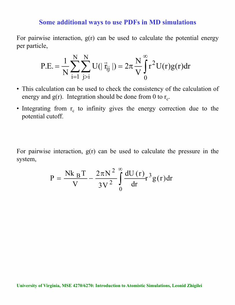
• This calculation can be used to check the consistency of the calculation ofenergy and g(r). Integration should be done from 0 to rc.

• Integrating from rc to infinity gives the energy correction due to thepotential cutoff.

For pairwise interaction, g(r) can be used to calculate the potential energyper particle,

0

2N

1i

N

ijij dr)r(g)r(Ur

V

N2|)r(|U

N

1.E.P

For pairwise interaction, g(r) can be used to calculate the pressure in thesystem,

dr)r(grdr

)r(dU

V3

N2

V

TNkP 3

02

2B

Some additional ways to use PDFs in MD simulations

correlation functions and their application for the 1...

Documents