CORRELATION OF FINITE ELEMENT FREE VIBRATION

PREDICTIONS USING RANDOM VIBRATION

TEST DATA

JEFFREY A. CHAMBERS

Bachelor of Science in Aerospace Engineering

Tri-State University

May, 1989

submitted in partial fulfillment of requirements for the

degree

MASTER OF SCIENCE IN ENGINEERING MECHANICS

at the

CLEVELAND STATE UNIVERSITY

June, 1994

https://ntrs.nasa.gov/search.jsp?R=19950010843 2018-06-20T15:58:24+00:00Z

This thesis has been approved for the

DEPARTMENT OF ENGINEERING MECHANICS and

the College of Graduate Studies by

__miM_n_irpers°n

Date

Dr. Paul A. Bosela / Department of Engineering Technology

_/,_/9 4--Date

Dr. Majid Rashidi / Department of Mechanical Engineering

o_-- 3/-_

Date

__,.v-_,-__._',_Dr. Omar M. Ibrahim / Structural Dynamics Engineer

Analex Corporation

Date

ACKMOWLEDGEMEMTS

I would like to acknowledge the efforts of my entire

thesis committee; Dr. Bellini, Dr. Bosela, Dr. Rashidi, and

Dr. Ibrahim. All have been very supportive and giving of

their time in helping to advance the development of my thesis

topic. I would like to extend special thanks to Dr. Bellini

for his conscientious help during both my thesis research and

supporting course work. Additionally, I would like to thank

those people at NASA Lewis Research Center who have given

freely of their time to aid in the development of this thesis.

CORRELATION OF FINITE ELEMENT FREE VIBRATION

PREDICTIONS USING RANDOM VIBRATION

TEST DATA

JEFFREY A. CHAMBERS

ABSTRACT

Finite element analysis is regularly used during the

engineering cycle of mechanical systems to predict the

response to static, thermal, and dynamic loads. The finite

element model (FEM) used to represent the system is often

correlated with physical test results to determine the

validity of analytical results provided. Results from dynamic

testing provide one means for performing this correlation.

One of the most common methods of measuring accuracy is by

classical modal testing, whereby vibratory mode shapes are

compared to mode shapes provided by finite element analysis.

The degree of correlation between the test and analytical mode

shapes can be shown mathematically using the cross

orthogonality check.

A great deal of time and effort can be exhausted in

generating the set of test acquired mode shapes needed for the

v

cross orthogonality check. In most situations response data

from vibration tests are digitally processed to generate the

mode shapes from a combination of modal parameters, forcing

functions, and recorded response data.

An alternate method is proposed in which the same

correlation of analytical and test acquired mode shapes can be

achieved without conducting the modal survey. Instead a

procedure is detailed in which a minimum of test information,

specifically the acceleration response data from a random

vibration test, is used to generate a set of equivalent local

accelerations to be applied to the reduced analytical model at

discrete points corresponding to the test measurement

locations. The static solution of the analytical model then

produces a set of deformations that once normalized can be

used to represent the test acquired mode shapes in the cross

orthogonality relation.

The method proposed has been shown to provide accurate

results for both a simple analytical model as well as a

complex space flight structure.

vi

7

TABLE OF CONTENTS

Chapter

I. INTRODUCTION

i.i Background

1.2 Objective

1.3 Scope

II. THEORETICAL DEVELOPMENT

2.1 Fundamental Dynamic Relationships

2.2 Preparation of Model

2.3 Calculation of Static Mode Shapes

2.4 Correlating the Mode Shapes

2.5 Automating the Process

III. CORRELATION PROCESS

3.1 Demonstration I

3.2 Demonstration II

IV. DISCUSSION

4.1 Summary and Conclusions

4.2 Recommendations for Further Study

REFERENCES

Page

1

4

6

8

I0

16

22

24

27

48

76

78

8O

\,

vii

APPENDICES

A - MSC/NASTRANDMAPListing

B - Cantilevered Beam Model

C - STDCE Experiment Package

81

88

ii0

viii

LIST OF TABLES

Table

I.

II.

III.

IV.

V.

VI.

VII.

VIII.

Comparison of Analytical and Test

Eigenproblem Results

Peak Response Values

Response Amplification Values

Acceleration Orientations

Equivalent Local Accelerations

Peak Response Data at Selected

Frequencies

Response Amplification Values at

Selected Frequencies

Accelerometer/Node Association

Page

35

42

43

44

45

69

70

73

ix

LIST OF FIGURES

Figure

2.1

3.1

3.2

3.3

3.4

3.5

3.6

3.7

3.8

3.9

3.10

3.11

3.12

3.13

3.14

3.15

3.16

Typical Response PSD Plot

Cantilevered Beam Analytical Model

High Fidelity Cantilevered Beam Model

Comparison of Test and Analytical

Frequencies - Cantilevered Beam Model

Excitation PSD at Large Mass

Response PSD at One-Third Span

Response PSD at Two-Thirds Span

Response PSD at Full Span

STDCE Flight Experiment Structure

STDCE Flight Experiment Structure

STDCE Flight Experiment Structure -Finite Element Model

STDCE Flight Experiment Structure -Finite Element Model

STDCE Flight Experiment Structure RandomVibration Test Levels

STDCE Flight Experiment Structure ResponseAccelerometer Locations

STDCE Flight Experiment Structure Mode 1 -

66.5 Hz

STDCE Flight Experiment Structure Mode 2 -71.1 Hz

STDCE Flight Experiment Structure Mode 3 -88.1 Hz

Page

15

28

34

36

37

39

40

41

50

51

52

53

55

56

58

59

6O

x

3.17

3.18

3.19

3.20

3.21

3.22

3.23

STDCE Flight Experiment Structure Mode 4 -

108.3 Hz

STDCE Flight Experiment Structure Mode 5 -

112.7 Hz

STDCE Flight Experiment Structure Mode 6 -

122.2 Hz

STDCE Flight Experiment Structure Mode 7 -

163.2 Hz

STDCE Flight Experiment Structure Mode 8 -

186.6 Hz

Sample Control and Response Measurements

Comparison of Test and Analytical Frequencies

61

62

63

64

65

67

71

xi

NOMENCLATURE

A

a

B

C

D

E

Y(t),F

f

G

g

I

I

K

L

M

PSD

Q

v

X(t),X

x

Cross sectional area

Local acceleration

Damping matrix

Cross orthogonality matrix

Intermediate matrix

Modulus of elasticity (flexural)

Dynamic force vector

Cyclic frequency

Intermediate matrix

Acceleration due to gravity

Identity matrix

Bending moment of inertia

Stiffness matrix

Element length

Mass matrix

Power spectral density

Response amplification factor

Power Spectral Density function

Displacement

Generalized displacement

Displacement

xii

A

v

P

Frequency response function

Eigenvalue

Poisson's ratio

Mass density

Eigenvector or eigenvector matrix

Circular frequency

Subscripts

A

a

f

G

I

O

o

s

T

Analytical related matrix

Active set

Displacement set

Generalized matrix

Input

Output

Omitted set

Iteration

Test related matrix

r,

xiii

CHAPTER I

INTRODUCTION

i.i BackqrouDd

During the engineering development cycle of

structural/mechanical systems, finite element models are often

used to provide insight into the static and dynamic response

characteristics of the system. Given the broad assumptions

made during the finite element modeling process, there is a

need to verify the accuracy of the modeling techniques

employed. The validity of these math models is usually

substantiated through static or dynamic tests conducted on the

engineered system. Results taken from these physical tests

are compared with analytical results provided by the finite

element model (FEM) under the same boundary and loading

conditions.

Probably one of the most common methods used to validate

a finite element model is through the use of modal testing and

2

correlation [i]. With this technique, the physical test

specimen is fixtured to represent its working environment, or

may be suspended in such a manner as to simulate free

restraint condition, and is subjected to a known forced

excitation (or simultaneous excitations). The response of the

system to this excitation is measured at various points about

the structure. The response data gathered is then analyzed by

making a transformation from physical (spacial) coordinates to

modal coordinates and the frequency response characteristics

of the system are generated mathematically by observing the

relationships between the forcing functions, response data,

and known modal parameters. This allows the generation of

mode shapes at resonant frequencies of the structure that can

be compared to the frequencies and mode shapes provided by the

analytical model.

The mode shapes generated from the physical test can be

mathematically compared to those from analysis by a number of

methods, with one of the more popular being the cross

orthogonality relation

[c] [¢.] (i.I)

where [C],_ is the cross orthogonality matrix correlating the

i-th analytical mode shape with the j-th test mode shape [2].

Matrices [_,] and [¢,] represent the assemblage of analytical

and test acquired mode shapes, respectively, while [MA] is the

analytically derived mass matrix.

3

Under ideal correlation where the test and analysis mode

shapes correlate identically, the resulting cross

orthogonality matrix appears as a unit diagonal matrix. Under

more realistic situations where the degree of correlation is

less than ideal, the degree of variation between the two sets

of mode shapes is identified by the density and magnitude of

the off-diagonal terms appearing in the cross orthogonality

matrix. Generally, satisfactory correlation is obtained if

the cross orthogonality matrix possesses no off-diagonal terms

exceeding 0.20 indicating twenty percent miscorrelation

between the i-th analytical and j-th test mode shapes.

Unfortunately, the process of modal testing can be quite

expensive and time consuming. It is not uncommon for the

modal test to consume many hundreds or thousands of man-hours

to set up, conduct, and post-process the data. It also

requires the use of specialized digital processing equipment

and software that may not always be available to the engineer.

This can make the correlation process somewhat prohibitive for

smaller scale engineering projects.

The process of correlating a finite element model can be

optimized if it may be done without the testing required with

the modal technique. In the case of space flight hardware,

this optimization could be realized if the frequency response

information needed from the test article could be provided by

means of the random vibration data that is normally acquired

during the flight qualification process. Random vibration

4

testing is usually required in the engineering process to

prove the system's structural and functional survivability

when subjected to the anticipated flight environment. This is

in sharp contrast to the modal technique which is necessitated

by the desire to validate the analytical assumptions.

Consequently if the engineering assumptions can be quantified

by the random vibration test, additional resources need not be

allocated for a separate modal survey.

Normally, the random vibration response data is not

accepted as valid correlation input since it only shows the

existence of resonance but in its raw form does not provide

any insight into the mode shape present at the resonant

frequency. In essence, the resonant frequency indicated by

the random response data may ideally match a frequency

provided by analysis yet contain a completely different mode

of vibration.

1.2 Obiective

Consider a scenario in which the random vibration data

gathered at a discrete number of spatial locations on the test

article is reduced to provide peak response and amplification

data for a limited number of primary frequencies indicated by

the test data and assumed to correspond with predetermined

analytical frequencies. These analytical frequencies at which

correlation is sought could be selected from the free

5

vibration analysis to represent the fundamental system

frequencies. This can easily be accomplished by selecting

modes in which there is significant mass participation.

Assuming that for any of these predetermined frequencies if

the structure were subjected to static loads equivalent to

those generated by the flight random vibration environment,

some sort of deflected shape could be expected. It stands to

reason therefore that since the random vibration test provides

local accelerations at discrete spacial locations and

frequencies the analyst should be able to surmise a deflected

shape for any of the resonant frequencies chosen from the test

data.

Given Power Spectral Density (PSD) output from a random

vibration test, peak response and amplification values can be

extracted for any number of selected frequencies. By use of

basic dynamic relationships, this response and amplification

data can be used to generate equivalent local accelerations

corresponding to the accelerometer locations and directions

monitored during the testing event. Assuming that these

equivalent local accelerations possess the proper orientations

and magnitudes, when applied to the FEM and a static analysis

performed, a static deformation is produced resembling the

mode shape expected at the frequency from which the response

values were taken. This static deformation can then be mass

normalized in the same manner as an eigenvector would be to

form a static or "pseudo' mode shape. This static mode shape

6

can then be used in the cross orthogonality correlation,

taking the place of the test acquired mode shape that would

have been generated via the modal technique. By carrying out

this procedure, a set of static mode shapes can be generated

from the frequency response characteristics of the physical

model without the need for any additional testing above that

done in the normal flight qualification process.

1.3 S._ope

This thesis provides a detailed method for accomplishing

the dynamic to static transformation which allows for the

generation of the static or "pseudo' mode shapes.

The equations governing the correlation process, from the

basic eigenproblem through the cross orthogonality check are

outlined to examine their relevance to the process. A

discussion is also presented on the preparation of both the

analytical model and random vibration test data. This

includes the reduction of the analytical model to those same

degrees of freedom observed in the vibration test as well as

the reduction of the random vibration data to the parameters

required in the calculations. The calculation of the static

mode shapes, their mass normalization, and comparison with the

mode shapes provided by the free vibration analysis is

presented in detail.

Lastly, the correlation process is demonstrated in full

7

for both a simplistic cantilevered beam model as well as for

an actual article of space flight hardware. The results of

both examples indicate that the process generates accurate

system mode shapes and provides a greatly abbreviated

correlation method.

THEORETICAL DEVELOPMENT

2.1 Fundamental Dynamic Relationships

The basic response characteristics (for both free and

forced vibration) of a mechanical system can be expressed by

means of the frequency response function (FRF). This

mathematical relation contains the mass, stiffness, and

damping properties of the system and can be used to evaluate

the frequency of vibration as well as the relative

displacements of the points within the system. In terms of

the spacial model, the mechanical system is described by mass,

stiffness, and damping properties

[_ b_+ [B] b_+ [_ Ix_:_F(t) ) (2.1 )

Considering the response to be a time varied function and

with the presence of damping the complete solution to be

complex, the FRF of the mechanical system can be written in

8

9

terms of the modal properties of frequencies and eigenvectors

(mode shapes).

x(t)=xe i_t (2.2)

(-_ [_ +i(_ [B] + [K] )xei_t=Fe_=F(t) (2.3)

: 3 : (2.4)

The preceding FRF represents a single term in the

complete FRF matrix that describes all modal properties of the

system. Ewins [i] provides a detailed development of the FRF

and its relevance in vibration testing.

The response of the system to random excitation is a

function of the total FRF and the source excitation. If this

input excitation is a time varied function of acceleration and

is considered to be a random process with a uniform spectral

density, S,(_), then the spectral density response, So(m), may

be represented by the following function

so(m) 12s ( ) (2.5)

Given the Power Spectral Density (PSD) function above

[3], it is evident that the response of a mechanical system to

a random excitation is dependent upon the full complement of

frequency response functions used to describe the mechanical

I0

system. Realization of this dependency enables the

transformation from random response characteristics back to

static response characteristics as proposed in the correlation

process. In the modal method, the frequency response function

is operated on directly to provide the system mode shapes.

The process to be developed uses the response as provided by

Equation 2.5 to generate the system mode shapes. It is

important to note, however, that the response provided by the

random response function contains all of those same frequency

response characteristics present in the modal method.

Although the origin, development, and theories behind the

frequency response and power spectral density functions are

very important in the analysis of dynamic systems, their

direct applications have very little impact on the development

of the process at hand. It is left up to the reader to become

familiar and comfortable with the mathematical origins of

these topics.

2.2 Preparation of Model

The correlation process deals with three varying levels

of fidelity representing the same mechanical system. The

physical test specimen represents a continuum system while the

analytical model represents the continuum system through

significantly reduced degrees of freedom. Thirdly, the

Ii

testing process gathers response data at a discrete number of

points (and directions) that represents still yet a further

reduction in the active degrees of freedom when compared with

the already reduced analytical model. Consequently in working

with the analytical and test models there needs to exist a

correspondence for those active degrees of freedom coincident

to both. Generally this means that the positioning of

accelerometers on the physical specimen are judiciously

selected so that the response measurements can accurately

represent the dominant response characteristics of the

structure. The positioning of these accelerometers can be

greatly aided by studying the predictions provided by the

analytical model. The analysis can provide great insight into

the system modes containing significant amounts of mass

participation as well as indicating spacial locations where

maximum dynamic deflections occur. Using this information to

place the accelerometers increases the likelihood of observing

the peak response characteristics during the testing event.

However, in the reverse process of applying measured data

to the analytical model in performing the correlation process,

it is also desirable to reduce the many degrees of freedom

present in the model to those same degrees of freedom which

were measured in test. Doing so allows a one-to-one

correlation between the analytical and physical properties.

When using MSC/NASTRAN for the analysis, this reduction in

active degrees of freedom can be accomplished through Guyan

12

(static condensation), Generalized Dynamic Reduction, or

component modal synthesis. The Guyan reduction method will be

used throughout this work. In the terminology of MSC/NASTRAN

[4] the degrees of freedom in the displacement set (x_) are

partitioned into the active set (x°) and the omitted set (Xo}.

The active set is that set remaining after condensation on

which the analysis is performed. Partitioning of the spacial

system is performed such that properties of the full structure

are maintained after condensation. In short, the reduction of

the free vibration problem is done in the following manner

[_e]b_+ [Bee]b_+ [Kf_]_=_01 (2.5)

(2.6)

(2.7)

(2.8)

[Goa]=- [Kj -_[f_] (2.9)

tx2= EG_]_2 (2.10)

13

= IGor] L_,}(2,11)

[G_] C-o2[Mff]+i_ [Bf_]+[Kf_]] [G_] L_O}(2.12)

which results in the final set of equations for the reduced

model (system)

[__2[Maa]+i_ [Ba,]*[Ka.]]_2={0} (2.13)

For a forced vibration problem, the static condensation

presented above takes some liberties with the time dependency

of the force vectors involved. But for the free vibration

problems presented in the correlation problem, these

assumptions pose no degradation in the solution process.

Therefore, the Guyan Reduction methods used by MSC/NASTRANcan

be used without concern. Alternately, Generalized Dynamic

Reduction may also be employed (which retains all factors in

the force vectors) with the same results being obtained.

Regardless of the method employed, either method allows for

the reduction from the full set of active degrees of freedom

to a set corresponding with the test measurement points and

directions.

During the testing event, acceleration response data are

14

gathered and processed to provide a set of PSD curves for each

accelerometer on the test specimen as well as those

accelerometers mounted on fixturing which provide a control

feedback loop to the excitation equipment. These PSD curves

generally appear as shown in Figure 2.1, one existing for each

DOFrecorded, providing acceleration response data in terms of

acceleration squared per unit frequency (g2/Hz) versus cyclic

frequency (Hz). When biaxial or triaxial accelerometers are

used, two or three such PSD curves appear for the same

discrete spacial location at which the accelerometer is

attached. This enables the engineer to observe response in up

to three translational directions at any given point on the

structure. In general, only translational accelerations are

measured since the measurement, processing, and application of

rotational accelerations is seldom used.

The random response data can provide a means of

identifying principle modes of vibration. Each set of data

(in reference to a given excitation) can be evaluated to

indicate principle modes excited by the input energy.

Generally, the response data can indicate a primary mode of

vibration by numerous appearances of distinct peaks at the

same frequency. Once a number of these modes have been

identified as being primary system modes or local modes of

interest, the peak values for each can be recorded from the

set of PSD curves. Amplification data can be calculated from

the response data at each of these frequencies by dividing the

15

III I I I 'r"l IIII i--4.11l:_r.. I

-III I I I I I

o

o(.q

m

| ml

IIII I I I

ooo

IIII I I I II

oo 14

01

III I ! I I I II

o

o

oo

o

oo

-- 0

o

ul

i N

- _

o

o

0rM

•

r-t

U

16

response PSD by the input PSD (from the control

accelerometers). For a given DOF and frequency the associated

amplification, or quality factor, may be calculated as

Qi = PSDres; (2.14)PSDi_u:

2.3 Calgulation of Static Mode Shapes

Once the test data has been reduced to a set of

frequencies, peak PSD and amplification values, the

corresponding static or 'pseudo' mode shapes can be calculated

using the analytical model.

With the reduction of the analytical model to the degrees

of freedom measured in test, as demonstrated earlier, the

apparent mass and stiffness of the FEM are given by matrices

[Mo°] and [Ku]. In order to produce statically deformed

shapes from this mass and stiffness, the peak PSD and

amplification values must be transformed to equivalent local

accelerations so that the static system of equations may be

solved

(2.15)

where {x}i represents the static deflection, or static mode

shape, resulting from the application of the equivalent local

17

accelerations {a),. The vector of equivalent local

accelerations {a)_ can be assembled from the individual peak

PSD and amplification values for each DOF present. The

transformation from dynamic response to equivalent local

acceleration is performed by use of Mile's equation [5]

ai:±3.0 (-_ )QiPSDi f (2.16 )

where a, = equivalent local acceleration

g = acceleration due to gravity

Q_ = amplification factor from test

PSDI = peak PSD value from test

f = frequency (cyclic) of interest

i = degree of freedom

This local acceleration term, a,, represents the

equivalent acceleration obtained for a single degree of

freedom on the test article at a single frequency point. If

the article is instrumented with five triaxial accelerometers,

then there will be fifteen such local accelerations calculated

and assembled to form a single acceleration vector, {a},.

Likewise, if four frequencies are chosen for correlation,

there will be four acceleration vectors, (a)_, assembled from

the test data.

The PSD and amplification factors involved come from test

data at a specific frequency value that may or may not be

18

identical to the frequency indicated by analysis but at which

the correlation is sought. To prevent introduction of error

from the test sequence (in reference to the frequency

discrepancies) it is preferable to use the frequency (f) as

provided by analysis. In other words, the correlation is

always going to be less than ideal since the test and analysis

models will never be identical. The intended purpose of the

correlation process is to compare the mode shapes of the two

and therefore it is desirable to avoid introducing additional

error into the calculations. A comparison of test and

analysis frequencies can be made on a much smaller scale as

will be demonstrated later. For this reason, the analytical

frequencies are used in the calculation of the eauivalent

_ocal accelerations.

One last step is required in the preparation of the test

data. The response data coming from test is assumed to be in

the proper relative magnitudes but contains no information

concerning the orientation, or direction, of the acceleration.

Some insight is needed to orient the applied accelerations so

that they are meaningful in the solution of the static system

of equations. The orientation of each acceleration can be

taken from the corresponding degree of freedom of the

eigenvector as predicted by the normal modes analysis. The

analytical eigenvector for each mode to be correlated can

easily be reduced to a directional vector containing positive

or negative values of unity to give the accompanying

19

acceleration vector the proper orientation at the reduced

nodal degrees of freedom.

From the static equations, the deformed shape, (x),

resulting from the application of the equivalent local

accelerations is performed by pre-multiplying both sides of

the static equation by the inverse of the reduced stiffness

matrix [Ku].

[Ka.]_ [Ka_]C_i= [f_] -i[_._]{a}i (2.17 )

(2.18)

This statically deformed shape is not unlike a raw

eigenvector having unbounded magnitudes of its components, and

may appear somewhat meaningless when first observed. However,

just as in an eigenanalysis, this deformed shape can be mass

normalized to provide the static or 'pseudo' mode shape.

{$__ b_ (2.19)

Ideally, it would appear that the series of equations

shown above could beapplied consecutively for all the vectors

of equivalent local accelerations representing the modes

desired to be correlated. But in fact if this were carried

out consecutively for a number of modes, it becomes evident

that the lower order modes have a large influence on the

2O

subsequent modes derived. The higher order modes exhibit

strong content of the lower modes, with the lowest mode

exhibiting the greatest influence.

To carry out the correlation process for modes other than

the lowest analytical mode presented, the influence of each

successive mode must be removed from the active set of

equations. This is easily performed by applying classical

matrix deflation techniques [6] to the system of equations.

Letting

[m] i: [Kaa] _i[Saa]i (2.20 )

and

_x_i: [D] i{a}i (2.21 )

Then by classical matrix deflation techniques, the

apparent mass and stiffness of the system excluding the

effects of vectors just iterated upon are established by

[D]i.,.",: [D] [Maa](2.22)

where _ and (_), are the eigenvalue and eigenvector as

provided by analysis, not test. Using the analytical values

again keeps the active mass and stiffness from becoming

contaminated with the error introduced by test. Also note

21

that to prevent the introduction of error, the eigenvalue and

eigenvector taken from analysis must be accurate enough to

prevent affecting downstream calculations.

If the analytical eigenvector is mass normalized as part

of its original processing, the denominator in the right side

of the equation takes on the value of unity by definition.

This allows the further simplification to

[D] i-i: [D] i-_i{_}i{_}T[Ma_] (2.23)

The solution of the second deflected shape in the series is

then

bdi÷ _: [D] i+1_a}i+1 (2.24)

This deformed shape is also mass normalized with respect

to the analytical reduced mass matrix to complete the

iteration and all subsequent static mode shapes are iterated

upon in the same manner.

It is important to reiterate that each successive mode

shape appearing in the analytical results must be swept from

the mass and stiffness matrices for the calculation of higher

order modes, even if that particular mode is not one to be

correlated. That is to say that if it is sought to correlate

the first, third, and fourth analysis modes, the second mode

must be swept from the system before the third and fourth

eigenvectors are calculated. Otherwise the presence of the

22

second mode will heavily influence the latter static mode

shapes.

2.4 Correlating the Mode Shapes

When all of the static mode shapes desired for

correlation have been calculated, the degree at which they

match the analytical mode shapes can be evaluated using any

number of methods, e.g. Modal Assurance Criterion, Cross

Orthogonality Criterion, etc. For the sake of demonstration

purposes, the cross orthogonality method has been chosen in

this thesis work.

expressed by

The cross orthogonality method can be

[c] : T[Maa] (2.25)

Where [_] is a matrix formed by assembling the eigenvectors

from analysis and [_T] is the matrix formed by assembling the

static or 'pseudo' mode shapes as calculated by the process

outlined above. The cross orthogonality matrix is a square

matrix where the diagonal terms represent the orthogonality

condition between each of the analytical and test

eigenvectors. If the i-th analysis eigenvector is identical

to the i-th test (pseudo) eigenvector, the i-th diagonal term

in [C] would be unity.

23

Therefore anything less than unity on the diagonal indicates

some level of skew between the analysis and test eigenvectors.

The off-diagonal terms represent the orthogonality

condition between the i-th analytical and j-th test

eigenvectors. By the principal of orthogonality, two

eigenvectors from the same eigenproblem must be perpendicular,

or orthogonal, to each other. Mathematically

{_,}[[Maa]{_]:0.0 (2.27 )

Therefore for ideal correlation between the analytical

and test models, the cross orthogonality matrix would appear

as a unit diagonal matrix. Realistically, where the

correlation between the analytical and test models is not

ideal the diagonal terms will become less than unity while the

off-diagonal terms will increase from zero. If the

correlation experienced is less than acceptable, the finite

element model can be "tuned' to gain more accurate

distributions of mass and stiffness. Iterations on the FEM

can be followed by recalculation of the static modes shapes

and the cross orthogonality matrix. The vibration testing

need only be conducted once since the same data is used for

each iteration on the finite element model. Usually,

satisfactory correlation has been achieved when the absolute

values of diagonal terms are greater than 0.90 and the

24

absolute values of the off-diagonal terms are limited to 0.20

or less. These limits are usually applied for those modes

deemed principal system modes or for local modes of particular

interest.

2.4 Automating the Process

A Direct Matrix Abstraction Program (DMAP) alter has been

written for Version 67.5 of MSC/NASTRAN [7] to carry out the

sequence of operations presented above. This DMAP alter uses

the analytical model, once reduced with Guyan or Generalized

Dynamic Reduction, to calculate the static mode shapes in the

same run sequence as a free vibration analysis is performed.

The DMAP statements are compiled in the MODERS module where

MSC/NASTRAN performs the real eigenvalue analysis. The user

is required to input matrices assembled from the vectors of

peak PSD and amplification values (Q) as well as a listing of

the analytical modes to be correlated. Peak PSD and

amplification values are entered via the DMI bulk data entry

cards (PSD and QUAL) while the list of modes to be correlated

are entered via a DTI entry (MODELST). The user is also

required to input several constant parameters to describe the

acceleration due to gravity (GRAY), maximum number of modes

predicted by analysis (NMAX), number of modes to be matched

(NMODES), and number of reduced degrees of freedom (NTEST).

25

The latter three values are used for partitioning the various

matrices assembled internal to MSC/NASTRAN. The user is also

required to disable the internal resequencing routine within

MSC/NASTRANso that no transformation between the internal and

external node numbering schemes is implemented. This helps to

prevent application of the external accelerations to wrong

internal degrees of freedom.

The DMAP alter recovers the reduced analytical mass and

stiffness matrices, Mu and Ko°, as well as the eigenvalue and

eigenvector matrices from the modal analysis. These

eigenvalue and eigenvector matrices are partitioned and

reduced for the modes to be correlated as indicated in the DTI

MODELST entry. The reduced eigenvector matrix is partitioned

term by term and the directional orientation of each DOF is

determined. A matrix (NDIR) is then assembled using these

directional orientations. The test data is then read and the

equivalent local acceleration matrix is formed by using Mile's

relation with the information provided.

The static mode shapes are calculated and mass normalized

as demonstrated earlier. After each static mode shape is

calculated, the influence of the corresponding analytical mode

shape is swept from the reduced mass and stiffness matrices.

Any intermediate modes not chosen for correlation are also

swept from the system before subsequent higher order static

mode shapes are calculated. The resulting matrix of static

mode shapes (PHITST) is automatically printed for the user.

26

Lastly, the reduced analytical eigenvector, reduced analytical

mass, and static mode shape matrices are used to perform the

system cross orthogonality calculation. The resulting cross

orthogonality matrix (COC) is also printed for the user.

A complete listing of the DMAP alter is given in Appendix

A.

CHAPTER III

CORRELATION PROCESS

3_I Demonstration I

For purposes of developing the correlation process, a

simple cantilevered beam model was used as the baseline

system. The analytical model is a cantilevered beam as shown

in Figure 3.1 consisting of four (4) nodes with two degrees of

freedom per node, one translational and one rotational. The

nodes are connected by three Bernoulli-Euler beam elements

with consistent mass and stiffness [8] as given below

[156 22T 54 -13L]

42o) / $4 13L 1s6-22L Il-13L -3L 2 -22L 4L2J

(3.1)

27

28

Y

AI¢

|

I I !0.1m _ 0.1m _ 0.1 m

_i_ _i _

....... _ X

/I--T E = 7o.o _Paf /

///_i _0 v = 0.33

.010 m@ = 2700 kg/m 3

___ I = 5.0 X I0 -I0 m 4--_ 0.006 m A = 6.0 X 10 -5 m 2

FIGURE 3.1

Cantilevered Beam Analytical Model

29

12 6L -12 6L I

EI 6L 4L 2 -6L 2L 2

[fi] :(_) -12 -6L 12 -6Z I

6L 2L 2 -6L 4L 2j

(3.2)

Substituting the geometric properties of the beam,

assembling the connectivity, and condensing out degrees of

freedom associated with the cantilevered restraint, the mass

and stiffness matrices appear as follows

[Maa] =3.85xi0 -5

"312 00

0

54

-I

0

0

00 0.08 1

00 1.30 312

30 -0.03 0

00 0.00 54

00 0.00 -I

30 -0 03 0

00 0 00 54

O0 0 08 1

00 1 30 156

30 -0 03 -2

0.00 54 00 -i 30

00 0

00 -i

30 -0

00 -2

20 0

0 00 0 00 _

00

30

O3

20

O4

(3.3)

840.00 0.00 -420 00 21 00

00 0

00 0

00 2

00 -21

00 0

70 0

00 -420

80 -21

00 420

70 -21

0.00 2.80 -21

-420.00 -21.00 840

21.00 0.70 0

o.oo o.oo -42o0.00 _ 0.00 ' 21

0 O0

O0

0.00

0.00

00 21.00

00 0.70

00 -21.00

00 1.40

(3.4)

For free-vibration, the basic eigenproblem can be given as

[Maa] kxJ'--to " (3.s)

30

Assuming the solution is harmonic in nature,

xi=Xcos (_ t-=) (3.6)

_ =-_Xsin (_ t-s) (3.7)

R_:-_2Xcos (_ t-a) (3.8)

Therefore the complete solution is

-_2Xcos (_ t-_) [Maa] +Xcos (_t-_) [faa] :{0f (3.9)

[[K_a]e2 [Ma.]]_dcos(e c_) =(0} (3.10)

[[K_] _ [_] ]L_:(0} (3.11)

For which the nontrivial solution is

det[ [Kaa] __2 [Maa]]=0 (3.12)

Using inverse iteration [6] as the solution scheme and the

Rayleigh quotient to force convergence of the eigenvalue

[D]_:[Kay][i[M.,.]i (3.13)

31

(3.14)

(.x.÷1}= Iv'_*1}

VI{v.+IV[M,,,.]Iv._lJ(3.15)

and the associated eigenvalue is

Iv.÷_[M,,_]Ix2(3.16)

Upon satisfactory convergence of the eigenvalue, the

final eigenvector can be normalized with respect to the system

mass (mass normalization).

{_A}i- {Vs+1} (3.17)

Subsequent eigenvectors and eigenvalues are found in the

same manner once the system is shifted to remove the influence

of the present mode. Therefore

1 T

[D],._=[D]_-"_(¢,,};(¢_h[_,] (3.18)

Performing the series of iterations on the analytical

model produces the following results

32

I 329.8 1.304e4 1.041e5 5.278e5 1.870e6 7.430e6'2.89 18.36 51.35 115.6 217.6 433.8

1.5021 -5.3845 6.7827 2.4709 2.7984 2.3954

=27.358 -53.667 -50.501 -315.713 521.238 245.6734.9630 -3.8654 -5.9809 1.1416 -4.9303 3.7505

AL' 39 .591 90.048 -38.548 323.470 342.850 690.579

9.0740 9.1282 9.1159 -9.8090 -10.6002 19.9162

41.635 145.594 241.534 -418.042 -702.697 1990.912

(3.19)

The validity of the eigenvectors calculated can be

reinforced by examining the orthogonality conditions present.

By definition of mass orthonormality,

associated with distinct eigenvalues

following relation

[4'] T[.,._ [4,1= [11

the eigenvectors

must satisfy the

(3.20)

where [I] is the real identity matrix.

operation

Carrying out the

[4',,] _'[_.j [4',,] -"

1 0000 0.0000 0 0000 0 0000 0.0000 0 0000"

0

0

0

0

0

0000 1.0000 0

0000 0.0000 1

0000 0.0000 0

0000 0.0000 0

0000 0.0000 0

0000 0

0000 0

0000 1

0000 0

0000 0

0000 0.0000 0

0000 0.0000 0

0000 0.0000 0

0000 1.0000 0

0000 0.0000 1

0000

0000

0000

0000

0000

(3.21)

All errors in the orthogonality test were on the order of

10 -7 indicating that the eigenvectors satisfy the

orthonormality constraint.

The test or physical

33

system for this demonstration

problem was simulated with a higher fidelity model (to imitate

a continuum system). An MSC/NASTRAN model was created with

sixty-one nodes, again with two degrees of freedom per node,

and sixty CBAR structural elements. Coupled mass formulation

was employed as in the analytical model. This model is shown

in Figure 3.2.

Initially, a normal modes analysis was performed on this

'test' model to compare the resulting frequencies with those

from the lower fidelity analytical model. The comparison of

eigenvalues and cyclic frequencies is shown in Table I.

As can be seen in the comparison, the lower fidelity

analysis model is significantly over-stiffened inthe higher

modes. The stiffening effect of the analytical model is shown

graphically in Figure 3.3. The systematic deviation from the

ideal line shows the uniform mathematical stiffening created

by the dramatic reduction in degrees of freedom associated

with the analytical model.

The eigenanalysis of the 'test' model was followed with

a random vibration analysis. The original model was augmented

by attaching a large (5000 kg) mass to the support node

applying a random acceleration excitation (Figure 3.4) to this

mass. The excitation was applied in the translational (Y)

direction to force bending response in the beam.

34

¥

A

T

72_i/jr/jr/jr//r//r//

r/ °

r//F/Ir//,.//r//,,//r//

f

I I I

Analytical Model

i i i0 • ,

I I Ii i ii i ii i

i,Test, Modei® ®\

-- Rigid Connection

k._ 61 Nodes

Large Mass

with Input PSD Applied

60 CBAR Elements

FIGURE 3.2

High Fidelity Cantilevered Beam Model

35

TABLE I.

Comparison of _hnalytical and Test Eigenproblem Results

Eigenvalue Frequency(Hz)

ModeAnal.

6

329.8

13305.3

T_t

329.7

12950.1

I01.5e3

Anal. Test %Diff

2.89 2.89 0.00

18.36

51.353 i04.1e3

4 527.8e3 389.9e3 115.6

5 186.9e4 i06.5e4 217.6

237.8e4 433.8743.0e4

18.11

50.71

-1.42

-1.25

99.37 -14.0

164.3 -24.5

245.4 -43.4

36

500.0

400.0

Nq-

,_ 300.0r..

o"

LL200.0

I--

100.0

0.00.0 100.0 200.0 300.0 400.0

Analysis Frequency, Hz

500.0

FIGURE 3.3

Comparison of Test and Analytical Frequencies - Cantilevered

Beam Model

37

N

dO9D.

1.000

0.100

0.010

0.001

10 100 1000 10000

Frequency, Hz

FIGURE3.4

Excitation PSD at Large Mass

38

Structural damping equal to ten percent of critical

damping (Q = 5) was included in the structure and was held

constant throughout the frequency range of zero to two

thousand Hertz. The translational response Power Spectral

Densities were recovered at the three nodes corresponding to

the node locations present in the analysis model (excluding

the support node). These PSD plots are shown in Figures 3.5,

3.6 and 3.7. The peak response values at resonant frequencies

were recorded from the analysis and are summarized in Table

II .......

By dividing each of the response predictions by the input

(control) acceleration, theresponse amplificationvalues can

likewise be tabulated for each active degree of freedom. This

set of amplification factors is shown in Table III.

Referring to the matrix of eigenvectors from the

analytical model (see Eq. 3.19) the directional attributes of

each DOF in each mode can be determined. The nodal

directional coefficients are shown in Table IV.

Using Mile's relation as presented earlier, the

combination of peak response, amplification, and orientation

are used to establish the set of equivalent local

accelerations. Note that the frequencies established by the

analytical model are used in the calculation of these

accelerations. These accelerations are shown in Table V.

Applying these equivalent local accelerations to the

analytical model using the process outlined earlier and mass

39

i_ "_ .L6 t

R

F

Y- _-2 *

2 t

5 IriS÷0 2

1R-3 t

6 t

2 • ./

/IE-4 _ )(]8

/1E-5

5 81E÷0 2

(

/

5 81._-1 2

flI

JK

/

5 SI_+2 2

I ,:I

1IIR

K

J

I v..

5 I11E-3 2

"'_x

_8

_I_-3

_4

_2

_Z_-4

.r .1E-5

FIGURE 3.5

Response PSD at 0ne-Third Span

40

_5RATI0N 2

PS

Y

D 5 L_____ __IREC

T 2 _0N

re- 3 _.

8 _

5 t

1.E-4

8

5

2 _ Xi

J1E-58 +

5 f

5 B1E÷0 2 5 81E+l 2 5 B1E+2 2

.... AX

/!,/

/X

tLI

t

1

5 81E÷3 2

_

(

5 SlE+4

_8

_5

*IE-2

÷5

,,-LE- 3_8

_5

_2

_lE-4_8

.5

+IE-5

+5

2

2 5 81E+0 2NCDE 41

HIGH FII_LITY _ BY_M

_J5 81E+3

+2

_-lE-6

FIGURE 3.6

Response PSD at Two-Thirds Span

41

L 6ER

P 2

F

Y

I._-2I 8RE 6

I 40N

1"_.-3 't

8

6

4

2 t

1_.- 4 +

6 ,t-

,.//2 _

1.I_-5 /*

5 IrlL_o 2

//

5 81E.,-1 2 5 IIZ_+2 2

L_F\_I

5 8_2+3 2

.8

*6

*2

.i_-2

____ _ +8

-6

*2

\,

I

÷6

+2

*IE-4

+8

*2

FIGURE 3.7

Response PSD at Full Span

42

TABLE II.

Peak Response Values

Freq/DOF

2.89 18.11

Peak PSD Values (g2/IIz)

164.3 245.4

Input 2.890e-4 1.881e-3 1.288e-2 5.290e-3

21T2 8.689e-4 1.029e-2 9.372e-3 1.919e-3

21_ 0.0 O.0 0.0

5.595e-3

0.0

1.799e-2

0.0

41T2 5.950e-3

0.0

3.012e-2

0.0

41R3

50.71 99.37

1.300e-2 1.500e-2

4.675e-2 4.908e-3

0.0 0.0

3.365e-2 2.146e-3

r.m

0.0 0.0

8.031e-2 4.531e-2

0.0 0.0

61T2

6.99_3

0.0

2.477e-2

0.061R3

6.339e-3

0.0

1.243e-2

0.0

43

TABLE III.

Response Amplification Values

Response Amplification Values

Freq/

2.89 18.11 50.71 99.37 164.3 245.4_F

21T2 3.001 5.470 3.596 0.327 0.728 0.363

21R3 0.0 0.0 0.0 0.0 0.0 0.0

41T2 19.360 3.163 2.588 0.143 0.143 1.198

41R3 0.0 0.0 0.0 0.0 0.0 0.0

61T2

61R3

62.249

0.0

16.013

0.0

6.178

0.0

3.021

0.0

1.923

0.0

2.350

0.0

44

TABLE IV.

Acceleration Orientations

AccelerationOrientations

l_eql .......

2.89 18.11 50.71 99.37 164.3 245.4DOF

21T2 1.0 -i.0 1.0 1.0 1.0 1.0

21R3 1.0 -i.0 -I.0 -i.0 1.0 1.0

41T2 1.0 -i.0 -i.0 1.0 -I.0 1.0

41R3 1.0 l.O -I.0 1.0 1.0 1.0

61T2 1.0 1.0 1.0 -l.O -i.0 1.0

61R3 1.0 1.0 1.0 -I,0 -i.0 1.0

45

TABLE V.

Equivalent Local Accelerations

EquivalentLocalAccelerations(m/s2)

Freq/

2.89 18.36 51.35 115.6 217.6 433.8DOF

21T2 3.203 -37.498 108.375 15.892 44.932 20.269

21R3 0.(] 0.0 0.0 0.0 0.0 (].0

41T2 20.637 -21.682 -78.007 6.949 -33.536 66.956

41R3 0.0 0.0 0.0 0.0 0.0 0.0

61T2 66.356 109.761 186.174 -146.719 -i18.754 131.292

61R3 0.0 0.0. 0.0 0.0 0.0 0.0

46

normalizing each resulting vector with respect to the reduced

analytical mass matrix, the following static mode shapes can

be derived.

fi

329.8 1.331e4 1.041e5 5.278e5 1.870e6 7.430e6

2.89 18.36 51.35 115.6 217.6 433.8

1.473 -5 322 6 819 2 306 3 525 -2.395

27. 046 -52

4.940 -3

40. 083 88

9.128 9

42. 523 149

912 -48

934 -6

439 -34

251 8

021 230

600 -353

018 1

436 331

940 -7

603 -189

950 576

962 -3

998 591

070 -I

772 156

020 -245.673

009 -3.751

330 -690.579

709 -19.916

038 -1990.91

(3.22)

As demonstrated earlier, the orthogonality condition of

the eigenvectors calculated can be evaluated using Equation

3.20.

[4>T] -"

I 000

0 006 1

0 000 0

0 000 -0

0 000 0

0 000 0

0 006 0 000

000 0

0i0 1

004 0

000 0

000 0

0.000

010 -0.004 0.000 0

000 0 .006 0 .007 0

006 Io000 -0.074 -0

007 -0.074 1.000 -0

001 -0.073 -0.402 1

0.000 0 000

000

001

073

402

000

(3.23)

The orthogonality results shown above indicate that

static eigenvectors calculated do experience some error,

particularly with respect to the orthogonality between the

fifth and sixth modes. The remaining modes appear to modestly

satisfy the orthogonality constraint. The fifth and sixth

47

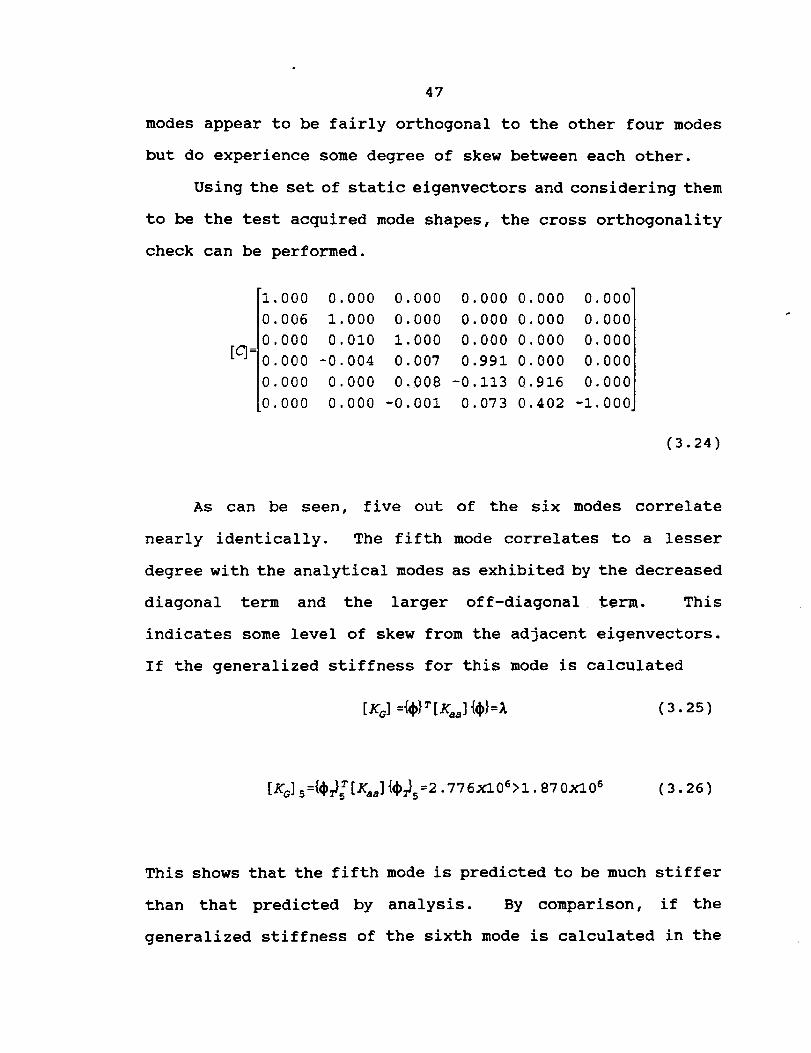
modes appear to be fairly orthogonal to the other four modes

but do experience some degree of skew between each other.

Using the set of static eigenvectors and considering them

to be the test acquired mode shapes, the cross orthogonality

check can be performed.

[g=

1 000 0 000

0 006 1 000

0 000 0 010

0 000 -0

0 000 0

0 000 0

0.000

0.000

1.000 0

004 0.007 0

000 0.008 -0

000 -0.001 0

0 000 0 000

0 000 0

000 0

991 0

113 0

073 0

000

000

000 0

916 0

402 -I

0 000'

0 000

0 000

000

000

000

(3.24)

As can be seen, five out of the six modes correlate

nearly identically. The fifth mode correlates to a lesser

degree with the analytical modes as exhibited by the decreased

diagonal term and the larger off-diagonal term. This

indicates some level of skew from the adjacent eigenvectors.

If the generalized stiffness for this mode is calculated

[KG] :_} T[Kaa]{¢}:I (3.25)

[KG],:{4')_"[K_,_,]{4'_},--2."7"76_ 0_>_.s'7ox_o_ (3.26)

This shows that the fifth mode is predicted to be much stiffer

than that predicted by analysis. By comparison, if the

generalized stiffness of the sixth mode is calculated in the

48

same manner

[KG] 43024 06-7.43020 06 (3.2?)

This sixth mode shape is nearly identical to that predicted by

analysis.

Overall this model would be considered to be well

correlated even with the presence of the larger off-diagonal

term relating to the fifth mode. Nearly ninety-one percent of

the total effective mass is present in the first four modes

correlated, with only four percent occurring in the fifth and

sixth modes combined. This indicates that the principle

vibratory modes are well represented by the static mode shapes

that were generated by process.

Formatted input and output from the MSC/NASTRANanalyses

of the high fidelity beam model are given in Appendix B.

9.2 DemoNstration II

Although the process has been demonstrated on a small

scale theoretical model, the entire process is intended to be

used during the engineering development cycle. Therefore, the

correlation process will also be applied to an actual space

flight structure for which the finite element modeling and

random vibration test sequences have already been performed.

49

The structure in question is a NASA space flight structure

that flew aboard Space Shuttle Columbia during the First U.S.

Microgravity Laboratory (USML-I) Spacelab Mission in 1992.

The package is approximately 19 inches wide, 36 inches tall,

26 inches deep, and weighs approximately 300 pounds. The

primary structural component is a large aluminum plate

machined with integral stiffeners to form a waffleplate, or

stiffened panel. This waffleplate supports various optical

components and the experiment test chamber. The waffleplate

is in turn supported by a framework of large channel sections

running front to back at all four corners. The front and rear

faces of the package are constructed of aluminum sheet that

form shear panels to tie the various structural components

together. Once mounted in the Spacelab module, the entire

structure is supported by the front shear panel and four

brackets attached to the primary channels at either of the

four rear corners. Several photos of the flight system are

shown in Figures 3.8 and 3.9.

An MSC/NASTRAN finite element model was constructed

during the engineering design process to serve as both the

dynamic and stress model for the system. Various views of

this finite element model are shown in Figures 3.10 and 3.11.

The model consists of plate and offset bar elements to form

the waffleplate structure with concentrated masses used to

represent those components attached to the waffleplate. The

rest of the primary structure is modeled using beam elements

5O

FIGURE 3.8

STDCE Flight Experiment Structure

51

FIGURE 3.9

STDCE Flight Experiment Structure

52

FIGURE 3.10

STDCE Flight Experiment Structure Finite Element Model

53

FIGURE 3.11

STDCE Flight Experiment Structure Finite Element Model

54

to represent the primary channel sections and various

stiffeners, while plate elements to represent the front and

rear shear panels. A separate study of the mass properties

showed the model to conform well with the actual structure in

both mass and center of gravity.

During the flight qualification process the Experiment

Package was rigidly fixtured and subjected to random vibration

testing at the maximum expected flight levels [9]. The input

spectra are shown in Figure 3.12. Three separate tests were

conducted, one in each of the three primary coordinate

directions with single axis base excitation. Response

acceleration measurements were taken at seven discrete

locations on the structure. Four of the accelerometers were

triaxial accelerometers intended to measure in-axis response

as well as response in the two cross-axis directions. One

accelerometer was biaxial and the last two accelerometers were

uniaxial accelerometers mounted to the front and rear shear

panels and intended to measure the out-of-plane panel

response. The locations of these accelerometers are shown in

Figure 3.13. The seven accelerometers together allowed

response measurements in sixteen degrees of freedom. Input

excitation was measured by four triaxial accelerometers

attached to the test fixture, and the response of these four

accelerometers was averaged to form the control feed-back

scheme for the test.

To correlate this FEM, the model was first reduced to the

55

0.100

0.010N

!

O03Q.

0.001

10 100 1000 10000

Frequency, Hz

FIGURE 3.12

STDCE Experiment Structure Random Vibration

Test Levels

56

m

o

,--I

i-i c)

0

C_

57

same sixteen degrees of freedom at which response data were

measured during the vibration tests. This was done by

including those degrees of freedom corresponding to the

accelerometers (response only) in ASETI bulk data entries and

employing Guyan Reduction.

A preliminary modal analysis was conducted on the model

to identify the principal modes of vibration. A separate

MSC/NASTRAN alter [i0] was employed in which the modal

effective mass of each mode was calculated. This allows the

analyst to determine which modes may be considered primary

system modes and exclude from the correlation process local

modes where negligible system mass participates. These

neglected modes are often local plate modes or coupled modes

where several modes of vibration are closely spaced. A

frequency span from zero to two-hundred Hertz was swept for

all modes within the range. A total of eight modes appeared

in this range, varying from 66.5 to 186.7 Hertz. Mode shape

plots for these modes are shown in Figures 3.14 through 3.21.

These eight modes represent about forty-five, twenty-five, and

forty-five percent of the total effective mass participation

in the coordinate X, Y, and Z directions, respectively.

Although these modes represent only a minority of the total

effective mass, this frequency range in which they occur is

suitable for correlating the model. Modes I, 3, 4, 5, and 7

have been selected for correlation based on the large

effective mass content in each of the modes. The second and

58

FIGURE 3.14

STDCE Experiment Package Mode 1 - 66.5 Hz

59

Y _.x

!

FIGURE 3.15

STDCE Experiment Package Mode 2 - 71.1 Hz

6O

.=

L_

FIGURE 3.16

STDCE Experiment Package Mode 3 - 88.1 Hz

61

FIGURE 3.17

STDCE Experiment Package Mode 4 - 108.3 Hz

62

FIGURE 3.18

STDCE Experiment Package Mode 5 - 112.7 Hz

63

FIGURE3.19STDCEExperiment Package Mode 6 - 122.2 Hz

64

FIGURE3.20STDCEExperiment Package Mode 7 - 163.2 Hz

65

JL_

1

7

I_/

!

FIGURE 3.21

STDCE Experiment Package Mode 8 - 186.6

66

sixth modes were excluded from the correlation since they

contain less than one percent of the total effective mass.

The MSC/NASTRAN output listing for this effective mass

analysis is given in Appendix C.

To proceed with the correlation process, the modes

determined to be primary modes now need to be identified and

separated in the random vibration test data. This can most

easily be accomplished by examining and sorting the test data

based on peak PSD values and the number of degrees of freedom

where these values appear at the same frequency. Quite often

one particular set of data, with respect to the excitation

axis, provides a more discernable appearance of a fundamental

mode more than the other sets of data. The set of data from

which the data for the mode is taken doesn't necessarily

coincide with the primary response direction (or effective

mass direction) of the mode since the response mode may most

easily be excited by cross-axis input (such as with a

torsional mode). However, these strong system modes usually

stand out markedly over the less effective or coupled system

modes.

Figure 3.22 shows the averaged control and three response

PSD plots corresponding to a single triaxial accelerometer

affixed to the waffleplate. These plots were taken from the

seventeen plots that make up the data set from the X-axis

test. Here it is easy to see the existence of a resonance at

105.5 Hertz. The peak values at this frequency have been

67

!J

N gUU

m

IIIII it ] I Illll I I I I f]llll I I Ii

o ,,_+ •

lI,+

=

n Ill

¢::1 'i.-iIoo

(

\

It n

0

II1111 I l Illll I I I r lllPIfl ! I I J

0

b.i

I|1111 ! 1 I Illll| I I ! I|lfll ! 1 I• . , o

o),LJ

?O3

Q)

O)

("4 0

nO

W _

0t_.LJ

0U

i,--I

68

indicated to illustrate how a data set is assembled. For the

STDCE Experiment Package, the peak PSD response data for the

five modes of interest has been reduced from the full

complement of test data and is shown in Table VI.

Amplification values (Table VII) are computed in the same

manner as demonstrated earlier using the control and response

PSD values.

A graphical comparison of the selected test frequencies

with the analytical frequencies is given in Figure 3.23. This

shows the third mode (88.1 Hz) to be somewhat stiffened in the

actual structure from what is predicted by analysis. The

remaining modes are overly stiffened in the model as might be

expected. These frequency differences may be the direct

result from the reduction in active degrees of freedom in the

model but may also be the result of effects not accounted for

in the modeling and linear analysis, e.g. joint friction and

other various nonlinear effects.

Before the PSD and amplification parameters can be used

in the correlation process, they must be rearranged in the

proper sequence to match the nodal numbering in the analytical

model. This ensures that the resulting local accelerations

are applied to the proper node and in the proper translational

direction. With the MSC/NASTRAN nodal renumbering scheme

deactivated, the system matrices are assembled and processed

using the external node sequencing, relating the degrees of

freedom with the nodes in ascending order. Therefore when the

69

TABLE VI.

Peak Response Data at Selected Frequencies.

ANAL. FREQ. 66.5 88.1 108.3 112.7 163.2

ANAL. ORDER 1 3 4 5 7

TEST FREQ. 65.2 92.1 95.4 105.5 134.8

glX

M2Y

g3Z

H4X

0.0083

0.4217

0.0009

0.8254

0.0049

0.1695

0.5623

0.0442

0.0054

0.1695

0.6190

0.0402

M5Y 0.1957 0.0287 0.0301

M6Z 0.1695 0.4217 0.4870

M7Y 3.0142 0.2488 0.2738

MSY 0.0301 0.0147 0.0169

1.1007

0.3318

0.0506

0.1540

0.3625

0.0590

0.0037

0.2054

h ,,

I_9X O.0049 O.0054 O.0065 O.9085 O.1957

NIOY O.1540 O.0590 O.0464 I.9573 O.0909

M11Z O.0012 O.4642 O.5109 O.0075 O.0054

MI2Y 0.0191 0.0249 0.0249 0.0029 0.0037

MI3Z 0.0010 0.0866 0.0909 0.0075 0.0044

g14X O.0010 O.0013 O.0026 O.1287 O.0442

MI5Y 0.0165 0.0021 0.0020 0.0316 0.0079

M167, 0.0002 0.0196 O.0178 0.0001 0.0001

CONTROL 0.0154 0.0095 0.0095 0.0193 0.0205

0.2260 0.0301

0.1334 0.0422

0.0649 0.0001

0.0562 0.0162

7O

TABLE VII.

Response Amplification Values at Selected Frequencies

ANAL.FREQ.

ANAL.ORDER

TEST FREQ.

66.5

65.2

88.1

92.1

108.3

95.4

112.7

105.5

16

134.8

MIX 0.5390 0.5158 0.5684 57.0311 17.6829

M2Y 27.3831 17.8421 17.8421 17.1917 2.8780

M3Z 0.0584 59.1895 65.1579 2.6218 0.1805

J

M4X 53.5974 4.6526 4.2316 7.9793 10.0195

3.0211

44.3895

26.1895

1.5474

12.7078M5Y

M6Z

_Y

MSY

3.1684

51.2632

28.8211

1.7789

11.0065

195.7273

11.7098

6.9119

3.3627

2.91191.9545

1.4683

2.0585

0.0049

0.7902

M9X 0.3182 0.5684 0.6842 47.0725 9.5463

NIOY i0.0000 6.2105 4.8842 101.4145 4.4341

MllZ 0.0779 48.8632 53.7789 0.3886 0.2634

_I2Y I.2403 2.6211 2.6211 O.1503 0.1805

MI3Z O.0065 9.1158 9.5684 0.3886 0.2146

O.0649 0.2737 6.6684 2.1561NI4X

0.2105 1.6373

0.00521.8737

NI5Y

MI6Z

1.0714

0.0130

0.1368

0.2211

2.0632

0.3854

0.0049

71

N-r-

o¢,..

o"

i._

LI.

O_

I-

200.0

150.0

100.0

50.0

0.00.0 50.0 100.0 150.0

Analysis Frequency, Hz

200.0

FIGURE 3.23

Comparison of Test and Analytical Frequencies

72

PSD and amplification values are prepared in the DMI entries,

the values are entered according to the corresponding node

numbers in ascending order. Table VIII shows the node and

accelerometer association for the Experiment Package.

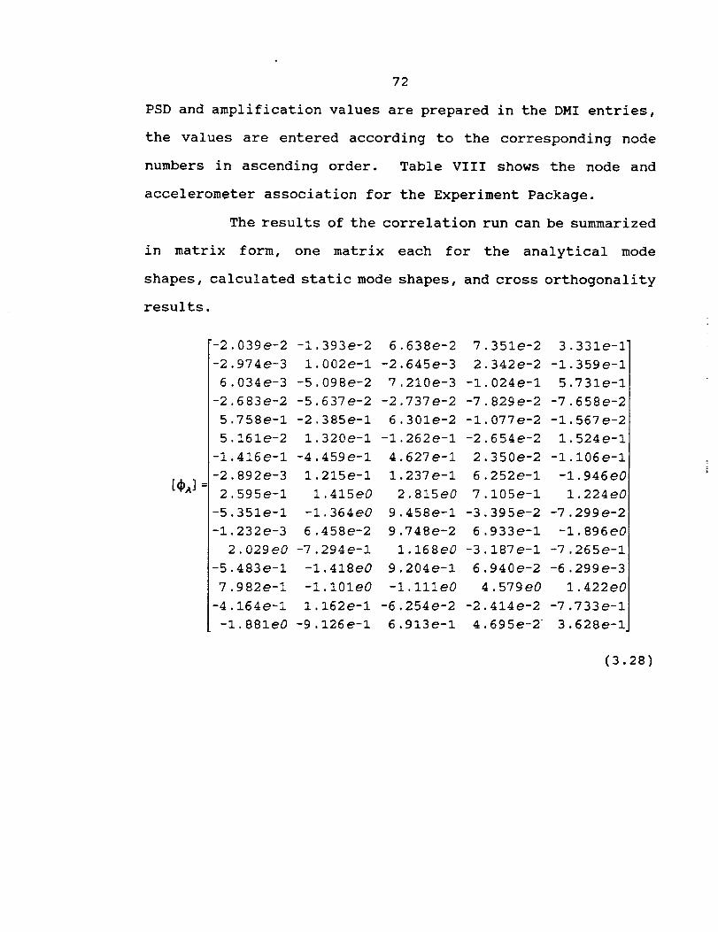
The results of the correlation run can be summarized

in matrix form, one matrix each for the analytical mode

shapes, calculated static mode shapes, and cross orthogonality

results.

=

"-2

-2

6

-2

5

5

-I

-2

2

-5

-i

.039e-2

.974e-3

.034e-3

.683e-2

.758e-I

161e-2

416e-I

892e-3

595e-I

351e-I

232e-3

-I 393e-2

1 002e-I

-5 098e-2

-5 637 e-2

-2 385e-i

1 320e-I

-4. 459e-i

1. 215e-I

1.415e0

-i. 364e0

6. 458e-2

2.029e0 -7.294e-i

-5. 483e-i -1.418e0

7. 982e-I -I. 101e0

-4. 164e-I 1. 162e-I

-1.881e0 -9.126e-i

6. 638e-2

-2. 645e-3

7. 210e-3

-2.737e-2

6. 301e-2

-I. 262e-I

4. 627e-I

1. 237e-i

2.8!5e0

9. 458e-i

9.748e-2

1.168e0

9. 204e-i

-I. ll!e0

-6. 254e-2

6.913e-I

7. 351e-2

2 342e-2

-I 024e-I

-7 829 e-2

-I 077 e-2

-2 654e-2

2 350e-2

6 252e-I

7 105e-I

-3 395e-2

6 933e-I

-3 187 e-i

6 940e-2

4. 579e0

-2. 414e-2

4.695e-2

3. 331e-I"

-1.359e-I

5.731e-I

-7. 658e-2

-i. 567 e-2

1.524e-I

-I. 106e-I

-I .946e0

1.224e0

-7.299 e-2

-I. 896e0

-7. 265e-!

-6.299 e-3

1. 422e0

-7.733e-i

3.628e-I

(3.28)

73

TABLE VIII.

Accelerometer/Node Association

Accel.

MIX

M2Y

M3Z

Node/DOF

603/TI

603/T2

603/T3

M4X 744/TI

M5Y 744/T2

M6Z 744/T3

M7Y 159/T2

Accel. Node/DOF

M9X 536/TI

MIOY 536/T2

MIIZ 536/T3

MI2Y 224/T2

MI3Z 224/T3

MI4X 149/TI

MI5Y 149/T2

M8Y 12/T2 MI6Z 149/T3

74

-I. 147 e-2

-2. 049 e-i

2. 179 e-I

1. 259e-i

-7 .776e-I

8 013e-2

-I 591e-I

-2 815e-I

3 011e-I

-3 267 e-i

-i 726e-I

1,975e0

-I. 826 e-i

1.775e0

-4.581e-i

-I, 426 e0

-2 501e-2

I 026 e-2

-5 I08e-2

-6 862e-2

-2 455e-i

1 543e-I

-5 262e-I

6 603e-2

5 862e-I

-i. 578e0

1.6 07 e-2

-i. 029 e0

-i. 636e0

-6. 563e-I

1.3i8e-i

-I. 048e0

4

-7

7

-I

5

-8

3

464e-2

058e-2

808e-2

850e-2

173e-2

025e-2

218e-i

7 671e-2

2.757e0

9.

9.

1

9.

-I. 452e0

-7. 347 e-2

6 °569e-i

-1.558e-I

5,764e-2

-2. 303e-I

-1.566e-2

-I. 052e-3

-5. 418e-2

2. 563 e-2

i. 157e0

3. 358e-I

239e-I 4. 217e-2

57 le-2 1.205e0

.157e0 -2.162e-i

811e-I 1.260e-i

3. 874e0

4. 477e-4

-2,237e-I

[c]=

0.9335 0.0000 0.0000 0.0000 0.0000"

-0.1854 0.9591 0.0000 0.0000 0.0000

0.0095 -0.2819 0.9955 0.0000 0.0000

0.1223 0.0120 -0.0661 0.9551 0.0000

0.1702 0.0143 -0.0045 -0.2811 0.9941

3 548e-I"

-i 175e-i

4 065e-I

-6 496 e-2

1 244e-2

9 557 e-2

-2 090e-2

-I ,913e0

1.220e0

-3. 074e-2

-I .964e0

-6.645e-I!

-I. i08e-i

1. 498e0

-6.70ie-i

4. 127 e-i

(3,29)

(3.30)

The process shows the model to correlate very well for

the modes selected. The sparse content of off-diagonal terms

and the relative magnitudes of the diagonal terms indicate

acceptable correlation between the analytical model and

physical system. The third and fifth analytical modes (second

and fourth selected) correlate to a lesser degree than the

other modes selected but still show satisfactory similarity.

75

Overall the analytical model may be considered to be a

relatively good approximation of the mass and stiffness

distributions of the continuum system. If a higher degree of

correlation was sought, the model could be 'tuned' by

adjusting mass and stiffness to provide more accurate mode

shapes and frequencies.

CHAPTER IV

DISCUSSION

4.1 Summary and ConclUSiQnS

A method has been outlined for substantiating the free

vibration predictions provided by finite element analysis

using random vibration data acquired via dynamic testing.

Power Spectral Density response data taken at a certain number

of spacial locations on the structure and corresponding to a

unique resonant frequency is used to generate a set of

equivalent local accelerations that can be applied to a finite

element model. Assuming that the finite element model is an

accurate representation of the continuum system, and therefore

possesses similar frequency response characteristics, these

equivalent local accelerations deform the structure in a

manner consistent with the mode of vibration from which they

were derived. This statically deformed mode shape can then be

compared with the free vibration mode shape at the

76

77

corresponding analytical frequency using modal techniques such

as the cross orthogonality method.

The process has been applied to a simple cantilevered

beam system using two analytical models: a high fidelity

model to simulate the continuum system and a significantly

lower fidelity model to serve as the analytical model.

Through random response analysis, response Power Spectral

Density and amplification levels were predicted over a large

frequency range to serve as data that would be acquired during

dynamic testing. These response levels were reduced at six

frequencies corresponding to the natural frequencies of

vibration predicted by the lower fidelity model. The reduced

data was used to generate sets of equivalent local

accelerations which were applied to the lower fidelity model.

The resulting system of static equations were solved and six

static deformations predicted, mass normalized, and compared

to the eigenvectors provided by the previous modal analysis.

Five of the six static mode shapes were found to correlate to

a very high degree with the analytical eigenvectors.

The same correlation process was also applied to a NASA

flight structure for which random vibration data had been

acquired in the flight qualification process. Five primary

system modes were chosen for correlation based on their mass

participation content. Three of the five modes evaluated were

found to correlate to a very high degree while the remaining

two correlated to a lesser but still acceptable degree. The

78

correlation of these two modes could be significantly improved

through the process of tuning the finite element model. The

tuning process, however, is beyond the immediate scope of this

thesis.

The results from both demonstrations indicate that the

process can effectively be used to generate the mode shapes of

the physical structure and thus correlate finite element

results. The application of this process has the potential

to substantially reduce the costs associated with correlating

such models by eliminating the need for additional testing

such as that required by classical modal techniques. All

information required to complete the correlation process can

be obtained during the normal flight qualification process.

4.2 Recomm@Ddations for Further Study

Even though the process developed here has been shown to

provide sufficient correlation results, it has not been

compared directly with results provided by alternate methods,

e.g. modal testing. The full justification of merits provided

by this method should be fully investigated by performing an

accepted correlation procedure in parallel with the proposed

procedure. Doing so would allow the comparison of test

79

acquired mode shapes from the two methods and also allow a

characterization of the mathematical error that is introduced

in the process that has been proposed.

8O

REFERENCES

•

•

•

.

•

o

•

•

.

i0.

Ewins, D. J., "Modal Testing: Theory and Practice",

Research Studies Press Ltd., Letchworth, Hertfordshire,

England, 1984.

Payload Flight Equipment Requirements For Safety-

Critical Structures, NASA JA-418, Revision A, Marshall

Space Flight Center, Huntsville, Alabama, 1989.

Crandall, S. H., and Mark, W. D., "Random Vibration in

Mechanical Systems", Academic Press, New York, New

York, 1963.

Gockel, M. A., Editor, MSC/NASTRAN - Handbook For

Dynamic Analysis, MacNeal-Schwendler Corporation, Los

Angeles, California, 1983.

Harris, C. M., and Crede, C. E., "Shock And Vibration

Handbook", Second Ed., McGraw-Hill, New York, New York,

1976.

Bathe, Klaus-Jorgen, "Finite Element Procedures In

Engineering Analysis", Prentice-Hall, Englewood Cliffs,

New Jersey, 1982.

User's Manual - MSC/NASTRAN Version 67, Volumes I and

II, MacNeal-Schwendler Corporation, Los Angeles,

California, 1991.

Craig, Roy R., Jr., "Structural Dynamics - An

Introduction to Computer Methods", John Wiley and Sons,

New York, New York, 1981.

Spacelab Payload ACCommodations Handbook, NASA

SLP/2104"2, Appendix B, Johnson Space Center, Houston,

Texas, 1986.

Rose, T., Alter to Compute Kinetic Energy and Effective

Weight, Proceedings of the MSC/NASTRAN World Users

Conference, 1988.

APPENDIX A

MSC/NASTRAN DMAP LISTING

81

82

55555555555555555555555555555555555555555555555555555555555555$$$$5$ Written by:$$$$$5$$$$$ Input :$$ PHIANL

$ MANL

$ KANL

$ NMODES

$$ NMAX

$$ NTEST

$ MODELST

$ GRAV

$ PSD

$ QUAL

$ NEWSEQ

$$$ Output :$$ coc$ PHITST

$ ACCEL

$ NDIR

$

January 1994

CROSS-ORTHOGONALITY CHECK OF ANALYTICAL MODE SHAPES

USING 'PSUEDO' STATIC MODE SHAPES DERIVED FROM RANDOM

VIBRATION DATA.

Jeffrey A. ChambersNASA Lewis Research Center

M/S 86-1221000 Brookpark Road

Cleveland, Ohio 44135

(216)433-8612

This DMAP alter is to be used with a Solution 103

Normal Modes Analysis. It was written and tested using

MSC/NASTRAN Version 67.5 for non-superelement models.

- Analysis Derived Mode Shapes

- Analysis Derived Mass Matrix

- Analysis Derived Stiffness Matrix- Number of Modes to be Matched

(PARAM, NMODES)- Number of Modes Provided by Analysis

(PARAM, NMAX)- Number of Test Points (PARAM, NTEST)

- Mode List for Correlation (DTI, MODELST)

- Acceleration Due to Gravity (PARAM, GRAV)

- Peak Response Matrix in g^2/Hz (DMI, PSD)

- Amplification Factor Matrix (DMI, QUAL)- Nodal Resequencing Deactivation

(PARAM, NEWSEQ, -i)

- Cross Orthogonality Matrix- Test Derived Mode Shapes- Nodal Acceleration Matrix

- Nodal Directional Matrix

$$$$$5555555555555555555555555555555555555555555555555555555$$ Compile MODERS processor just after OFP module.COMPILE SEMODES SOUIN=MSCSOU NOLIST NOREF

ALTER 2,25TYPE DB KJJ, MJJ, BJJ, USET, GOA, GOAT, KAA, DYNAMICS, KGG,

PCDBS, AGG, PVT, GPLS, SILS, SLT, DM, CASES, EQEXINS,

MATPOOL, GM, KOO, LO0, DIT, BGPDTS, CSTMS, EST, MPTS,

XYCDBS, LLL, KLL, ULL, EMAP, MAPS, ETT, PVTS, KFS, KSS,

83

KSF, KVV, EDT, GEOM2S, GEOM3S, ECTS, EPTS, INDTA, KELM,

KDICT, GPECT, VELEM, EQEXINX, ECTX, BGPDTX, SILX,

GEOM4S, VGFS, SPECSEL, GPDTS, MELM, MDICT, GEOMI,

GEOM2, GEOM3, GEOM4, EPT, MPT, SLIST, VACOMPR,

$ DYNAMICS ONLY

BGG, K4GG, MFF, MLR, MLL, MRR, CMLAMA, CMPHA, CMPHO,

MLAAI, MR, GOAQ, KLAA, MLAA, MAA, MAR, MEA, BAA, K4AA,

MGG,

$ PHASE 2

PHA, LAMA, PHFA, LAMAF, PHSA, LAMAS,

$ PHASE 3

PHG, PHQG, PUG, GPSF, OPHGI, OPHQGI, OPHEFI, OPHESI,

OPHEEI, OPHESMI, OPHESGI, OPHEEMI, OPHEEGI, PHGPS,

OPHNRGY, OPHGPFB, CASEDR, XYCDBDR, OPHGPSI,

$ EQUIV SCRATCH

MKAA, MMAA, OLB, PCDB, VAFS, XYCDB, EDOMX, CASECC $

ALTER 36,365

CALL MODERS MR, USET, DM, CASES, DYNAMICS, MMAA, MKAA, GPLS,

SILS, EED, EQEXINS, VACOMPR, DMI, DMINDX, DTI, DTINDX/

PHA,LAMA/

NORSET/ NOLSET/ 'MODES'/ ASING/ FALSE/ FALSE/ NOQSET $

COMPILE MODERS SOUIN=MSCSOU NOLIST NOREF

ALTER I,i$

SUBDMAP MODERS MR, USET, DM, CASES, DYNAMICS, MMAA, MKAA,

GPLS, SILS, EED,

EQEXINS, VACOMPR, DMI, DMINDX, DTI, DTINDX/

PHIA,LAMA/

NORSET/ NOLSET/ READAPP/ ASING/ CYCLIC/ SECND/ NOQSET $

ALTER 845

$ Input user specified response levels, amplification

$ levels, and listing of modes to be correlated. Input via

$ bulk data DMI and DTI cards.

DMIIN DMI,DMINDX/PSD,QUAL,,,,,,,,/$

DTIIN DTI,DTINDX/MODELST,,,,,,,,,/$

TYPE PARM,,I,Y,NMODES$

TYPE PARM,,I,Y,NTEST$

TYPE PARM,,I,Y,NMAX$

TYPE PARM,,RS,Y,GRAV$

TYPE PARM,,I,N,COUNT=I$

TYPE PARM,,I,N,PARTI$

TYPE PARM,,I,N,PART2$

TYPE PARM,,I,N,COUNTI$

TYPE PARM,,I,N,COUNT2$

TYPE PARM,,RS,N,PI2=I.570796335

TYPE PARM,,CS,N,ALPHA$

TYPE PARM,,RS,N,RADI$

TYPE PARM,,CS,N,MRI$

FILE CP=OVRWRT/RP=OVRWRT/AII=OVRWRT/AI2=OVRWRT$

FILE A21=OVRWRT/A22=OVRWRT/BII=OVRWRT/BI2=OVRWRT$

FILE B21=OVRWRT/B22=OVRWRT/CII=OVRWRT/CI2=OVRWRT$

FILE C21=OVRWRT/C22=OVRWRT/DII=OVRWRT/DI2=OVRWRT$

FILE D21=OVRWRT/D22=OVRWRT/KINV=OVRWRT/DEF=OVRWRT$

84

FILE ACCEL=OVRWRT/ACCELI=OVRWRT/MODEI=OVRWRT$

FILE DEFT=OVRWRT/XMODE=OVRWRT/COC=OVrWRT$

$ Echo user input of response levels, amplification levels,

$ and modes to be correlated.

MATPRN PSD,QUAL//$

TABPT MODELST//$

$ Retrieve and equivalence analysis matrices. GDR

$ stiffness, GDR mass, eigenvectors, and eigenvalues.

EQUIVX KXX/KANL/ALWAYS$

EQUIVX MXX/MANL/ALWAYS$

EQUIVX PHIX/PHIANL/ALWAYS$

LAMX,,LAMAILAMATI-I$

MATPRN KANL,MANL,PHIANL,LAMAT//$

$ Partition eigenvector and eigenvalue matrices for the

$ modes to be correlated. Modes to be correlated are

$ identified by DTI entry MODELST. There may be at most

$ as many modes requested as the number specified by

$ NMODES.

EQUIVX LAMAT/LAMTMP/ALWAYS$

MATGEN ,/LAMDA/7/I/5$

MATGEN ,/PHIRED/7/NTEST/I$

COUNT=ISDO WHILE (COUNT <= NMODES)$

PARAML MODELST//'DTI'/COUNT/I//S,N,PART$

PART 1=PART- 1$

PART2=NMAX-PART$

IF (PART = I) THEN$

MATGEN ,/CP/6/NMAX/PART/PART2$

MATGEN ,/RP/6/NMAX/PART/PART2$

ELSE$

MATGEN ,/CP/6/NMAX/O/PARTI/I/PART2$

MATGEN ,/RP/6/NMAX/O/PARTI/I/PART2$

ENDIF$PARTN LAMTMP,,RP/LAMTP,A21,AI2,A22/I$

PARTN PHIX,CP,/PHITP,B21,BI2,B22/I$

IF (COUNT > i) THEN$COUNTI=COUNT-I$

TRNSP LAMDA/TEMPI$

TRNSP LAMTP/TEMP2$APPEND TEMPI,TEMP2/TEMP3$

TRNSP TEMP3/LAMDATX$

EQUIVX LAMDATX/LAMDA/ALWAYS$APPEND PHIRED,PHITP/PHITX$

EQUIVX PHITX/PHIRED/ALWAYS$

ELSE$

EQUIVX LAMTP/LAMDA/ALWAYS$

EQUIVX PHITP/PHIRED/ALWAYS$

ENDIF$COUNT=COUNT+IS

ENDDO$

MATPRN LAMDA,PHIRED//$$ Create the nodal directional matrix NDIR by extracting

85

$ each term in PHIRED and selecting its directional

$ orientation (e.g. +i.0 or -i.0). Directional terms are

$ assembled in NDIR matrix of size [NTEST X NMODES].

EQUIVX PHIRED/NDIR/ALWAYS$

COUNTI=0$

DO WHILE (COUNT1 < NMODES)$

MATGEN ,/CP/6/NMODES/COUNTI/I$

COUNT2=0$

DO WHILE (COUNT2 < NTEST)$

MATGEN ,/RP/6/NTEST/COUNT2/I$

PARTN NDIR,CP,RP/AII,A21,AI2,AOLD/I$

NORM AOLD/ANEW/$

MERGE AII,A21,AI2,ANEW,CP,RP/NDIRI/I$

EQUIVX NDIRI/NDIR/ALWAYS$

COUNT2=COUNT2+I$

ENDDO$

COUNTI=COUNTI+I$

ENDDO$

MATPRN NDIR//$

$ Create the nodal acceleration vector ACCEL for each mode

$ by extracting each term from NDIR, PSD, QUAL and LAMDA

$ then solving Miles equation.

MATGEN ,/ACCEL/7/NTEST/NMODES$

COUNTI=0$

DO WHILE (COUNT1 < NMODES)$

MATGEN ,/CP/6/NMODES/COUNTI/I$

MATGEN ,/CPL/6/5/2/I/25

MATGEN ,/RPL/6/NMODES/COUNTI/I$

PARTN LAMDA,CPL,RPL/,,,FREQI/I$

COUNT2=O$

DO WHILE (COUNT2 < NTEST)$

MATGEN ,/RP/6/NTEST/COUNT2/I$

PARTN NDIR,CP,RP/AII,AI2,A21,NDIRI/I$

PARTN PSD,CP,RP/BII,BI2,B21,PSDI/I$

PARTN QUAL,CP,RP/CII,CI2,C21,QUALI/I$

PARTN ACCEL,CP,RP/DII,DI2,D21,DOLD/I$

SMPYAD QUALI,PSDI,FREQI,,,/RAD/3/I$

PARAML RAD//'NULL'////S,N,NOPG$

IF (NOPG = -i) THEN$

RADI=0.0

ELSE$

PARAML RAD//'DMI'/I/I/S,N,RADI$

ENDIF$

RADI=(3.0*GRAV*SQRT(PI2*RADI))

ALPHA=CMPLX(RADI)

ADD NDIRI,/ACCELI/ALPHA$

EQUIVX ACCELI/DNEW/ALWAYS$

MERGE DII,DI2,D21,DNEW,CP,RP/ACCELI/I$

EQUIVX ACCELI/ACCEL/ALWAYS$

COUNT2=COUNT2+I$

ENDDO$

COUNTI=COUNTI+I$

86

ENDDO$

MATPRN ACCEL//$$ Perform the static solution [KANL]_-I*[MANL]*{ACCEL} for

$ each mode selected to generate the 'psuedo" static mode

$ shapes. Each mode shape is mass normalized for the

$ correlation process. After each mode shape is generated

$ its influence in the remaining static solution is removed

$ by performing a deflation of the static matrix in the

$ form: [DEF]=[KANL]^-I*[MANL] - (LAMDA)^-I *[PHITST]^T

$ *[PHITST]* [MANL]. Intermediate modes not selected for$ correlation are also swept from the system using the

$ corresponding mode shape provided by analysis.

MATGEN ,/KINV/7/NTEST/NMODES$

MATGEN ,/PHITST/7/NTEST/I$

MATGEN ,/MODEI/7/NTEST/I$

MATGEN ,/DEF/7/NTEST/NMODES$

MATGEN ,/DEFT/7/NTEST/NMODES$

SOLVE KANL,/KINV/3$

MPYAD KINV,MANL,/DEF/0/I$COUNT=IS

COUNTI=I$

PARAML MODELST//'DTI'/COUNTI/I//S,N,PART$

DO WHILE (COUNT <= NMAX )$

IF (COUNT = PART) THEN$MATMOD ACCEL,,,,,/ACCELI,/I/COUNTI$

MPYAD DEF,ACCELI,/XMODE/O/I$

SMPYAD XMODE,MANL,XMODE,,,/MFSQR/3/I///I/O/O$

PARAML MFSQR//'DMI'/I/I/S,N,MR$

MR=I.0/SQRT(MR)$MRI=CMPLX(MR)$

ADD XMODE,/XTEMP/MRI$

MESSAGE //'CALCULATION OF STATIC MODE SHAPE = '/PARTS

IF (COUNT = i) THEN$EQUIVX XTEMP/PHITST/ALWAYS$

ELSE$

APPEND PHITST,XTEMP/XMODE$

EQUIVX XMODE/PHITST/ALWAYS$

ENDIF$

MATMOD PHIANL,,,,,/MODEI,/I/COUNT$

SMPYAD MODEI,MODEI,MANL,,,/NUMER/3////O/I/O$

PARAML LAMAT//'DMI'/I/COUNT/S,N,EIGVAL$

MESSAGE //'EIGENVALUE = '/EIGVAL$

EIGVAL=-I.0/EIGVAL$

ALPHA=CMPLX(EIGVAL)$

ADD DEF,NUMER/DEFT/(I.0,0.0)/ALPHA/O$

EQUIVX DEFT/DEF/ALWAYS$

COUNT=COUNT+ISCOUNTI=COUNTI+I$

PARAML MODELST//'DTI'/COUNTI/I//S,N,PART$

ELSE$MATMOD PHIANL,,,,,/MODEI,/I/COUNT$

SMPYAD MODEI,MODEI,MANL,,,/NUMER/3/I///O/I/O$

87

PARAML LAMAT//'DMI'/I/COUNT/S,N,EIGVAL$

EIGVAL=-I.0/EIGVAL$

ALPHA=CMPLX(EIGVAL)$

ADD DEF,NUMER/DEFT/(I.0,0.0)/ALPHA/0$

EQUIVX DEFT/DEF/ALWAYS$

COUNT=COUNT+IS

ENDIF$

ENDDO$

MATPRN PHITST//$

$ Perform the Cross Orthogonality computation for the modes

$ selected. Orthogonality is provided by [PHIRED]^T *

$ [MANL]*[PHITST].

MATGEN ,/COC/7/NTEST/NMODES$

SMPYAD PHIRED,MANL,PHITST,,,/COC/3/I///I/O/O$

MATPRN COC//$

MESSAGE //'CROSS ORTHOGONALITY COMPUTATION COMPLETE'$

ENDS

APPENDIX B

CANTILEVERED BEAM MODEL

- Eigenvalue Analysis, Input

- Eigenvalue Analysis, Output (Abridged)

- Random Response Analysis, Input (Abridged)

- Random Response Analysis, Output (Abridged)

88

89

SOL 103

TIME 4

CE_D

SEALL = ALL

SUPER : ALL

SET i00 : 21,41,61

TITLE = High FidelityCantileveredBeam Model

ECHO : SORT

SPC: 5

SUBCASE1

METHOD : 1

BEGIN BULK

P._9.1M AUTOSPCYES

PARAS COUP_SS 1

PAR_ WII4ASSi.

PARAM GRDPNT 0

EIGR 1 SI]6' O. 2000.

+ A _SS

PBAR 1 1 6.-5 5.-i0

CBAR 1 1 l 2 i.

CBAR 2 1 2 3 i.

CBAR 3 1 3 4 i.

CBAR 4 1 4 5 i.

CBAR 5 1 5 6 i.

6"BAR 6 1 6 7 i.

CBAR 7 1 7 8 i.

CBAR 8 1 8 9 i.

6"BAR 9 1 9 i0 i.

CBAR i0 1 i0 ii i.

CBAR ii 1 II 12 i.

CBAR 12 1 12 13 i.

6"BAR 13 1 13 14 i.

CBAR 14 1 14 15 i.

CBAR 15 1 15 16 I.

CHAR 16 1 16 17 i.

CBAR 17 1 17 18 i.

CBAR 18 1 18 19 i.

CBAR 19 i 19 20 i.

CHAR 20 1 20 21 i.

CBAR 21 I 21 22 i.

CHAR 22 1 22 23 i.

CHAR 23 1 23 24 i.

CBAR 24 1 24 25 I.

CBAR 25 1 25 26 i.

(:BAR 26 1 26 27 i.

CBAR 27 i 27 28 i.

CBAR 28 1 28 29 i.

CBAR 29 1 29 30 i.

CBAR 30 1 30 31 i.

CHAR 31 1 31 32 i.

CBAR 32 1 32 33 i.

CHAR 33 1 33 34 i.

20 +

i,

i.

i.

i.

i.

i.

i.

i.

i.

i.

i.

i.

i.

i.

I.

I.

i.

i.

i.

I.

i.

1.

1.

1.

1.

1

1

1

1

I

I

I

1

O°

O.

O.

O.

O.

O.

O.

O.

O.

O.

O.

O.

O.

O.

O.

O.

O.O.

O.

O.

O.

O.

O.O.

O.

O.

O.O.

O.

O.

O.

O.

O.

90

_AR

_AR

_AR

_AR

_AR

_._R

_AR

CUR

_AR

_._R

_AR

_AR

_._

_._

_AR

_TI

@ID

GRID

GRID

_ID

GRID

GRID

GRID

GRID

_ID

GRID

_ID

GRID

GRID

_ID

_ID

_ID

GRID

GRID

GRID

GRID

_ID

GRID

_ID

_ID

34

35

36

37

38

39

40

41

42

43

44

45

46

47

48

49

50

51

52

53

54

55

56

57

58

59

60

I

1

2

3

4

5

6

7

8

9

i0

ii

12

13

14

15

16

17

18

19

20

21

22

23

24

1

1

1

1

i

1

1

1

1

1

i

1

1

1

1

1

i

1

1

1

1

1

1

1

1

1

1

7.+7

34 35 i. i.

35 36 i. i.

36 37 i. i.

37 38 i. i.

38 39 i. I.

39 40 i. I.

40 41 i. i.

41 42 i. i.

42 43 I. I.

43 44 i. I.

44 45 i. I.

45 46 I. i.

46 47 i. i.

47 48 i. i.

48 49 I. I.

49 50 i. I.

50 51 i. i.

51 52 I. I.

52 53 I. i.

53 54 I. i.

54 55 I. I.

55 56 i. i.

56 57 i. i.

57 58 I. i.

58 59 i. i.

59 60 I. I.

60 61 I. i.

.3333332700.

O. O. O.

.005 O. O.

.009999O. O.

.014999O. O.

.019998O. O.

.024998O. O.

.029997O. O.

.034996O. O.

.039996O. O.

.044995O. O.

.049995O. O.

.054995O. O.

.059994O. O.

.064994O. O.

.069993O. O.

.074993O. O.

.079992O. O.

.084991O. O.

.089991O. O.

.09499 O. O.

.09999 O. O.

.10499 O. O.

.10999 O. O.

.114991O. O.

O°

O.

O.

O.

O.

O.

O.

O.

O.

O.

O.

O.

O.

O.

O.

O.

O.

O.

O.

O.

O.

O.

O.

O.

O.

O.

O.

91

GRID

GRID

GRID

GRID

GRID

GRIDGRID

GRIDGRID

GRID

GRID

GRID

GRID

GRID

GRID

GRID

GRID

GRID

GRID

GRID

GRID

GRID

GRID

GRID

GRID

GRID

GRID

GRID

GRID

GRID

GRID

GRID

GRID

GRID

GRID

GRID

GRID

SPCkDD

SPCI

SPCI

ENDDATA

25

26

27

28

29

30

31

32

33

34

35

36

37

38

39

40

41

42

43

44

45

46

47

48

49

50

51

52

53

54

55

56

57

58

59

6O

61

5

4

7

4

123456

1345

.119991

.124991

.129992

.134992

.139992

.144992

.149992

.154993

.159993

.164993

.169994

.174994

.179994

.184994

.189994

.194995

.199995

.204995

.209996

.214996

.219996

.224996

.229997

.234997

.239997

.244997

.249998

.254998

.259998

.264998

.269999

.274999

.279999

.284999

.29

.295

.3

7

1

2

O.

O.

O.

O.

O.

O.

O.

O.

O.

O.

O.

O.

O.

O.

O.

O.

O.

O.

O.

O.

O.

O.

O.

O.

O.

O.

O.

O.

O.

O.

O.

O.

O.

O.

O.

O.

O.

TBRU

O.

O.

O.

O.

O.

O.

O.

O.

O.

O.

O.

O.

O.

O.

O.

O.

O.

O.

O.

O.

O.

O.

O.

O.

O.

O.

O.

O.

O.

O.

O.

O.

O.

O.

O.

O.

O.

61

92

-K _ 4C "4(

4C 4C 4C -K

4C 4_ "K 4C

,,K "K "K -K

-K "K _ 4_ 4C"K -K

',K "K

r_ .K 4C-K 4¢

4C ,.K•K -K

4C 4C -IK 4C

-K .IK -I_ -K

o°..°_

_O

_ o__°_oooo_• ° ° _ • °

!

93

_oo

o_

÷÷÷

_o_

I K _ l_

q_

q_

q_c_

q_

c_÷

c_c_

c_

ll_ IK qK

v_q

X

r_

Dml

94

÷÷ ÷

O

O

r_

Z

rm_

0 ÷÷ _

0_1 O0

III!

95

! II

• . . .

• . . °

.°..

0 _ 0 _ 0

• -.. .io.

0 0 0

• ... °°°.

96

÷ + +

_D ('M

•--4 ('_ ('_

÷÷÷

I

('9

,,.°

(._

°°.°

I

O

°°°°

U

O

Z

O

°0°.

_ °.,.

II ii n ii

_N •

97

SOL iii

TIME 4

CEND

SF.&LL= ALL

SUPER = ALL

SET i00 --21,41,61,1,62

TITLE : High FidelityCantileveredBeam Model

SPC: 5

SUBCASE 1

SUBTITLE=RandomResponseAnalysis

MEIIDD = 1

FREQUENCY= 2

SDANP = 75

RA_ = 85

DLOAD=95

BEGIN BULK

tlttliitltlitliitliiitliitliittlttliiiiiiitliitltlitli

REMAINDEROF INPUTREMAINSUNCHANGEDBUT

BEEN OHITTEDHERE FOR BREVITY

tliiiiiitttli!IIIIIIIIitliiitttlttliiittttliiiiittlitiRBE2 99 62

CONM2 62 62

SPCLDD 5 4

SPCI 4 13456

SPCI 6 13456

SPCI 7 1345

FREQ2 2 O.1

FREQ 2 2.8900

+F O001A 456.334586.142

+F O001B 1949.59

DAREA 96 62

RLOAD2 95 96

TLBDMPI 75 Q

+T O003A O. 5.0

TABLED1 97

+T O000A O. I.

RANDPS 85 1

TABRNDI 86

+T O002A O. O.

+T 0002B I00. .015

+T 0002C ENDT

ENDDATA

2 1

5.+4

6 7

I

62

2 THRU 61

2000. 75

18.811150.713099.3774164.278245.403342.755+F0001A

732.182894.4571072.971267.731478.751706.03@ O001B

2 5.+4

97

2000. 5.0 ENDT

2000. I. ENDT

i I. O.

20. .002 40.

150. .015 500.

+T O003A

+T O000A

86

+T O002A

.008 55. .015 +T O002B

.003 2000. .00047+T 0002C

98

-K -K -K -K

.4_ .,K -K ..K

"_" "K '.K

• K ,,X _ -IK

,r

,°w°,,

!

.,,.,w

_ °°°w,.

_O

__._

O

O

• .... °

99

,'K "K "K

•4- ÷ "4"

•K 'K "K

° _ _ _

o..

o_

÷ ÷

C_I C_

C_ C_

o_ ip-4

C_ _ OCI

÷ ÷r._ _c_ c_c=, _,

c_ c_c_ c_

c_ c_

-K -K -K ._c

o.

r_

_N

r_

r._

_P

i00

X _

°°°°°°°°°°°°°°°°°ii(2_ CD _D _ZD _D _D CD CD _D _D _D CD {D _D CD _D _D

.

• O0 _ ,--I ,--I ,--I ('..1C..1 (',.1 ¢',.1 4_ ("._ ¢".1 _"} e"_ e"_ ("_ _'5 _2

_ ÷ + + + + + + + + + ÷ ÷ + + + _. =,: e_ e_

N N_==

I + + -i- + + + + + + + + + + + + +

i01

{.2

iiiiitJlllllllllllllllllllltlllll

_ oo..,...ooo.6.o

• • • o • • • • • • • •

II

102

m

o.ooooo,o,,,,ooo,oooo,,o .... o,.o.oo.

103

.0000.0o0.o..,0.0...

_ N

Z _ _

0

_Z _

mm

÷+

O r._

• N_

104

,,wo°oo,oo,oo,o°°o,,.,,.-o.,,to,o-,_

105

÷÷÷÷÷÷÷÷÷÷÷÷÷÷÷÷÷÷÷_÷_÷÷÷_÷÷÷÷÷÷÷÷÷_

106

.,.o.....,.-.-

..............

.4.4

_-m e,%

,.a

4- 4-

= _4M,-

_ -t- ÷

= _"

o,oeolo_o

107

......................... M_dMd_dd_d

108

109

.oooo.oo

+ + + + ÷ ÷ + -4-

_ N__ oI'_ o'-J ,_ L,n e,..-, e,,.- _, I_

• • • • o . o •

APPENDIX C

STDCE EXPERIMENT PACKAGE

- Eigenvalue Analysis, Input (Abridged)

- Eigenvalue Analysis, Output (Abridged)

- Correlation Analysis, Input (Abridged)

- Correlation Analysis, Output (Abridged)

ii0

iii

SOL 103

TIME i0

CDD

TITLE = STDCE EXPERIMENTPACKAGE- AS BUILT FLIGHTHAP/)WARE

SUBTITLE= NOREIL MODES A_ALYSIS- STATICCONDESATIONEMPLOYED

ECHO = SORT

SPC = 41

VECTOR(PLOT)= ALL

_THOD=I

DY]_RED=2

BEGIN BULK

EIGR 1 SINV O. 200. i00

÷ I _SS

DYNRED 2 200.

$ DOF ASSOCIATEDWITH ACCELEROMETERLOCATIONS/DOF

ASETI 123 603 744 536 149

ASETI 23 224

ASETI 2 159 12

$ PAPJ_4ETERSASSOCIATEDWITH EFFECTIVE_SS CALCULATIONS

P_/_ KEPRT 1

PA_AM EFWGT 2

PA_._ CHKSTIF1

PARAM CEKMASS1

$$ BEGINNINGOF EXPERIMENTPACKAGESTRUCTURE(C200)

$

## DUE TO ITS VOL_INOUS NATURE,THE BULK DATA INPUT FOR THE

# EXPERIMENTPACKAGEMODEL _ BEE_ OMITTED. THE COMPLETEMODEL

# CA_ BE OBTAINED FK)M THE AUTHOR.

#

$ PARAMETERSASSOCIATEDWITH THE MODAL SOLUTION

PAP,AM AUTOSPC YES

PARAM CO_P_(ASS 1

PARA]4 GRDPNT 0

P_ K6ROT 1000.

PARAM WT_ASS i.

ENDDATA

l-

112

('4_D

K*a

o

0 __

.,....

......

!

z_ M_d_d

Z

,-,m

o.o.o.

I

o011..

!

_ o

113

CD C) CD

CD CD CD

_ _ CD

CD CD ,-_

o,o

++÷

_NN

_NN

N r,.- t",_ _

• oe +

_,1 _,10 I",1

_MM! ! I

I

_X_

!

I++

• •

I

N _

_NN

II

+

_4

+

1%1

4-

.,--4

,--4

("_ ,--_ O0

! I

,.-* (-4 (_4

'aO e'% e'%

,--4

! !

4_ ._ 4c

,.a

,.-I

Z

114

,- 115

116

SOL103TIME10###,#,H#.Hh,li,##,l#h,Jl#I,,i.,,,,,,,,,H,##i,#,

CORRELATIONDMAP ALTER IS INSERTEDHERE

####HHH##I##II##I###II##I##I######HI#ll#########1#CI_II)

SET 100 = 603, 744, 536, 224, 149, 159, 12

TITLE: STI)CEEXPERIMENTPACKAGE- ASWILT FLIGI_B/el)WARESUBTITLE= NORMALMODES_ALYSISWITHCROSSORTHOGONALITYCHECKSEALL : ALL

SUPER = ALL

ECHO = SORT

SPC = 41

VECTOR = I00

HETID])=I

DYNRED:2

BEGIN BULK

lllllttÁtlltllllllltllll#tlt#111ttlltlltlllllllllltltl

REMAINDEROF INPUT RDt_INSUNCHANGEDBUT

HAS BEEN OMITTEDHERE FOR BREVITY

ltllllllllttllllll#1##ttlllltlllltllllllltlltllllll#1!I)MI PSI) 0 2 1

DMI PSD 1 1 .0301

.0191 .0010 .0049 .1540

.8254 .1957 .1695

_I PSD 2 1 .0147

.0249 .0866 .0054 .0590

.0442 .0287 .4217

DMI PSD 3 1 .0169

.0249 .0909 .0065 .0464

•0402 .0301 .4870

I_I PSD 4 i .0562

.0029 .0075 .9085 1.9573

.1540 .2260 .1334

DMI PSI) 5 1 .0162

.0037 .0044 .1957 .0909

.2054 .0301 .0422

DMI QUAL 0 2 1

DMI QIIAL 1 1 1.9545

1.2403 .0065 .3182

53.597412.707811.0065

DMI QUAL 2 1

2.6211 9.1158 .5684

4.6526 3.0211 44.3895

I_I QUAL 3 1

2.6211 9.5684 .6842

4.2316 3.1684 51.2632

D_I QUAL 4 1

0 16 5

3.0142 .0010 .0165 .0002

.0012 .0083 .4217 .0009

.0013 .0021 .0196 .2488

.4642 .0049 .1695 .5623

.2738 .0026 .0020 .0178

.5109 .0054 .1695 .6190

•0649 .1287 .0316 .0001

•0075 1.1007 .3318 .0506

.0442 .0079 .0000 .0001

.0054 .3625 .0590 .0037

0 16 5

195.727.0649 1.0714 .0130

10.0000 .0779 .5390 27.3831.0584

1.5474 .1368 .2211 2.0632 26.1895

6.2105 48.8632 .5158 17.842159.1895

1.7789 28.8211 .2737 .2105 1.8737

4.8842 53.7789 .5684 17.842165.1579

2.9119 3.3627 6.6684 1.6373 .0001

117

.1503 .3886 47.0725101.415.3886 57.031117.19172.62187.979311.70986.9119

DMI QUAL5 1 .7902 2.1561.3854 .0000 .0046.1805 .2146 9.54634.4341.2634 17.68292.8780.180510.01951.46832.0585

DTI,MODELST,O

DTI,HODELST,I,I

DTI,_DELST,2,3

DTI,MODELST,3,4

DTI,MODELST,4,5

DTI,MODELST,5,7

PARAM,_DES,5

PARA}{,_EST,16

PARAM,NMAX,8

PAR_/4,GRAV,386.4

PARAM NEWSEQ -I

ENDDATA

118

_ _ _ _ _ •

l _ •

0

Z _

ra_

It

_ 0

0

MMd_M_w!

...o..

..°...

119

4( -K 4(

O O+ 4" ÷

oooo_o o

o.,

00.

°_

_NNN

• o

I

dNN_X_

II|

,i,.

÷ .4-

¢M ,_,

I

I ÷

I

N _

I

4( 4(

4(

_D÷

_DU_

(',,)

_4

4-

C_

,6

_D

-4-

_4I

4(

•K 4( -K

÷

(%3

_4

4-

('v'1

,--4

(',3

4-

O%

,--4

,--4

4( 4( 4¢

-_: 4( -K

(,3,--4,..-4

e'% ,--_ O%

i !

•-4 ('%1 f_1_ CD _

,-4

l I

•K 4( 4(

120

o

M

_ _ °°°°°°°°N _ .÷÷+**÷. N

_ N_N _N N

_ _,

8

_D

121

w-

w-

e_

&:%

o<

,0

.m-

c_cDi 4-

e'% cDcD

_:_ oocD _D

cD

o0 oD

•..-4CD

CD

122

-I-

_0

,-4I

-I-

+.,

,-4I

oO

¢.%J

•4- 4-

,dD

(=_ ¢,4cD cD.4- .4-

o% Ix_f'q

I I

cD (_n

!

._P (,4

•4- -I-

-t.

N

,'4 '_I

•4- -I-

o%s.¢%r.--- ,4D

.4-

cO

e,_ ,,.O

,-4 _4I

CD

r.--

@,=1_D.4-

,P.-I

,.-4• •

Im_ ,--I!

('4CD CD

0%

I I

4- 4-

,4D

_4I

,4D

e-II

C_

(',,1

o<

@'4

4-

I=...,4DO_

+.,;<

r..-. ¢_

I I

,--, (',4

++.,

_O @,1

,--4

I

-4- -I-

N

,.4_:I

• -.I ,.-,

I

("4 (-4

+ 4-

123

4" "I"

,_ ,-, mm

_r

÷

N

_NI ¢

!

!

,,F

I

N

_4I

÷

!

4-

!

• • !_ ,d3 !

I II

! i

"r

"7'

÷ ÷

I

+ .4-

N _

N _

÷ ÷

I

o'_ o'3

I

4-

!

_ c_

°

,. o. • o •

II I I I I

o-

124

I! II II

++ +_ ++ ÷ +÷ +

II II II

÷÷ ÷+ ++ _+ +÷ _ ! '' ,,

++ +÷ +_ ÷ ÷÷ ÷

• • • •

I I I I I _ i

8 8 8 8 8 8 8 8

!

@

9

I

@

9

II

!

I Ii

_ N_Im.I

N NN

_ MM

N _

N

9

N

I

!

I

,--,_Or_ 00 !

r',-,I

I I

¢;

¢M

i

! I

i I

_ N

!

!

125

!

_4

I

_d

e4

I

Ie_

I t

I

| I

,

N

I !

! !

!

! !

I I

_ N

, , _

o • o • •

I I I I I

_D

F.1

N

0

I I

dM _|| |

NN NN

_ MM' 'N ' 'NNN_ NN =

N_ N_

NN _

|

! I

O _

!

!

I

I

,4!

,6I

!

!

@

_4

I

I

8 _

I

!

@

N

I

I II

!

!

!

!

I

\

127

129

+

+

!

I

'7'_ ,,...4

I

!

_,' ,-,

T-.-4 ,_-I _

! !

I ÷

!

4-

÷

I

'4- +

+ +_ e-',

X

8

+ +

"r

0+

¢=,

4-

0

.4-

4- +

¢=, _,

I

+ ÷

• •

I

4- +

CD

O

?-_ ??

4-

CD

CD

+

CDCDO

+

OO(:m

CD CD4- 4-

CDO

O CD

7,,-_

I

+ +

I I

+ .4-

+ +

+ +

+ +

++ ++

++ +÷

++

++

NN_ &N

X

_d!

+

¢=,+

÷

,,--4

?

÷

4-

_4I

!

+

• • o,

I I I II I

8

?

+

4-

I

+

(3%

!

+

+

+

+

?

4-

r_

!

4-

+

$I

130

\

131

Form Approved

REPORT DOCUMENTATION PAG E OMBNo.0704-0188PLy.ic.reportingb_J_._, for this.collectio(t..ofinformatkm._ estin_ted to average 1 hourper response, includingthe time for revte_ng tnstruchons,searching existingdata sources,g_nenng _ maJma0nln_lme _ neeoea. _ _ing .anorevle_ng !he .cc_.k)cllon,of information. Send oomrnentsregardlngth_ burden estimateor any other aspect o( thisCOl_Ct_ _ mvor.rn_on.jncLuomg Bugs. tlons__lorreo_uc_gthin Ipurden,to w.asn_ngtonHeaoquarlers Services, Directoratefor Inl.ormahonOIoetatiorlSa.ndRepotls, 1215 Jeffersonuavts Highway, _;une "IL-'XJ4.Arlington.VA Z'_-43¢SZ, and to the Off'co Of Managementano Buoget, PaperworkReducl_onProject(0704-0188), Washlngton, DC 20503.

1. AGENCY USE ONLY (Leave b/aRk) 2. REPORT DATE 3. REPORT TYPE AND DATES COVERED

November 1994 Technical Memorandum4. TITLE AND SUBTITLE 5. FUNDING NUMBERS

Correlation of Finite Element Free Vibration Predictions Using RandomVibration Test Data

6. AUTHOR(S)

Jeffrey A. Chambers

7. PERFORMING ORGANIZATION NAME(S) AND ADDRESS{ES)

9.

National Aeronautics and Space AdministrationLewis Research CenterCleveland, Ohio 44135-3191

SPONSORING/MONITORING AGENCY NAME(S) AND ADDRESS(ES)

National Aeronautics and Space AdministrationWashington, D.C. 20546-0001

WU-None

8. PERFORMING ORGANIZATIONREPORT NUMBER

E-9243

10. SPONSO_NG/MON_ORINGAGENCYREPORTNUMBER

NASA TM- 106787

11. SUPPLEMENTARY NO_i:_

This report was submitted as a dissertation in partial fulfillment of the requirements for the degree Master of Science inEngineering Mechanics to Cleveland State University, Cleveland, Ohio, June 1994. Responsible person, JeffreyA.Chambers, organization code 4320, (216) 433--8612.

12a. DIsiHIBUTION/AVAILABILITY STATEMENT 12b. DISTRIBUTION CODE

Unclassified -Unlimited

Subject Category 39

13. AB:_ i HACT (Maximum 200 words)

Finite element analysis is regularly used during the engineering cycle of mechanical systems to predict the response tostatic, thermal, and dynamic loads. The finite element model (FEM) used to represent the system is often correlated with

physical test results to determine the validity of analytical results provided. Results from dynamic testing provide onemeans for performing this correlation. One of the most common methods of measuring accuracy is by classical modal

testing, whereby vibratory mode shapes are compared to mode shapes provided by finite element analysis. The degree ofcorrelation between the test and analytical mode shapes can be shown mathematically using the cross orthogonality check.A great deal of time and effort can be exhausted in generating the set of test acquired mode shapes needed for the crossorthogonality check. In most situations response data from vibration tests are digitally processed to generate the modeshapes from a combination of modal parameters, forcing functions, and recorded response data. An alternate method is

proposed in which the same correlation of analytical and test acquired mode shapes can be achieved without conductingthe modal survey. Instead a procedure is detailed in which a minimum of test information, specifically the accelerationresponse data from a random vibration test, is used to generate a set of equivalent local accelerations to be applied to thereduced analytical model at discrete points corresponding to the test measurement locations. The static solution of the

analytical model then produces a set of deformations that once normalized can be used to represent the test acquired modeshapes in the cross orthogonality relation. The method proposed has been shown to provide accurate results for both asimple analytical model as well as a complex space flight structure.

14. SUBJECT TERMS

Random vibration; Modal analysis; Vibration; Vibration testing;Loads and vibration; Structures

17. SECURITY CLASSIFICATIONOF REPORT

Unclassified

NSN 7540-01-280-5500

18. SECURITY CLASSIFICATIONOF THIS PAGE

Unclassified

19. SECURITY CLASSIFICATION

OF ABSTRACT

Unclassified

15. NUMBER OF PAGES

14516. PRICE CODE

A0720. LIMITATION OF ABSTRACT

Standard Form 298 (Rev. 2-89)

Prescribed by ANSI Std. Z.39-18298-102