Corrosion: Simulating and Rendering

Stephane Merillou Jean-Michel Dischler Djamchid Ghazanfarpour

ENSIL - University of Limoges16 rue Atlantis 87000 Limoges - France

AbstractWeathering phenomena represent a topic of growing in-terest in computer graphics, and corrosion reactions areof great importance since they affect a large number ofdifferent fields. Previous investigations have essentiallydealt with the modeling and rendering of metallic pati-nas. We propose an approach based on simple physicalcharacteristics to simulate and render new forms of cor-rosion. We take into account ”real world” time and dif-ferent atmospheric condition categories with experimen-tal data. This allows us to predict the evolution of cor-rosion over time. The reaction is simulated using a ran-dom walk technique adapted to our generic model. Forrealistic rendering, we propose a BRDF and (color- andbump-) texture models, thus affecting color, reflectanceand geometry. We additionally propose a set of rules toautomatically predict the preferential starting locations ofcorrosion.

Key words: Rendering, corrosion, natural phenomena,texturing, BRDF.

1 Introduction

Real-world surfaces are often covered by lots of imper-fections due to various aging processes. To compute re-alistic images, it seems important to take into accountsuch processes by adding a time dependence to renderedscenes. Aging and weathering effects can take many dif-ferent forms such as dust accumulation, patinas, mois-ture, scratches, erosion, etc. But, only very few studieshave been proposed so far in computer graphics. Dustysurfaces were investigated by Blinn [1] and Hsu [12], tar-nished surfaces by Miller [20]. Dorsey [7] proposed amodel to take into account dirtiness brought by flow pro-cesses. In [24], Wong provided a geometry dependentmethod to represent dust accumulation, patinas and peel-ing. Weathering of stones has been studied in [8]. Re-cently, we introduced a technique to render individuallyvisible scratches appearing on old surfaces [19].

Usually, corrosion reactions can be divided into twomain categories: metallic patinas and rusty layers.Dorsey [6] proposed a first phenomenologic model torender metallic patinas based on a multiple layers ap-

Figure 1: Real corroded surfaces

proach. The surface alterations creating these layers arehandled by some specific operators and are controlled byspecific spreading techniques. To obtain realistic images,the reflectance and transmission of light through theselayers are computed with the Kubelka-Munk model [16].The modelling of corrosion patterns has been studied byGobron in [10]. Icart [13] proposed to render oxydationlayers appearing on materials by using multiple layersBRDF. Metallic patinas, as investigated in [6], consistof a sort of “protection” layer that avoids “too much”matter loss. It affects nearly only color and reflectance(at the human visible scale). On the other side, metalslike iron are affected by corrosion in a sort of “destruc-tive way”. Great amounts of matter can be wasted com-pared to patinable materials (such as copper), in particu-lar, holes can appear on the surface.In this paper, we propose a model to simulate and rendernew forms of corrosion that correspond to the second cat-egory. Our model affects the geometry of objects (“realholes” resulting from the matter loss can appear), as wellas its color and reflectance. In section 2, we propose abrief survey of corrosion. Our model, detailed in section3, permits in a first step to predict the starting locationsof corrosion by defining a set of generic rules. In order tocompute the “real” matter loss and to obtain aplausiblesimulation, we use a generic law fitting experimental re-sults given in [14]. Then, we describe our random-walk-

based spreading process, resulting in a “corrosion map”(three overlapping maps: a reflectance map, a color mapand height map). The map can be pasted and renderedon the object surface using usual texturing techniques ora more accurate virtual ray tracing technique [5] (thisis a general form of texture/bump mapping, taking intoaccount light and view dependance, as well as parallaxeffects and hidden surface removal on the bumps). Thecorroded parts reflectance is computed by modifying theparameters of the non-corroded surface BRDF: corrodedsurfaces are particularly rough and porous, thus greatlyaffecting the global reflectance (BRDF). This is an impor-tant issue in computer graphics since metals are usuallyshiny, while corrosion is rather not. Color is consideredeither using an approach based on a table of oxidationmaterials or empirically using color tables gathered fromreal-world examples (photos). Section 4 shows resultsobtained for different corrosion processes and differenttimes (given in years). Finally, we conclude this paperin section 5, and discuss some possible improvements ofour method as well as some future works.

2 Physics of Corrosion

2.1 IntroductionCorrosion can be defined as the deterioration of a mate-rial against its environment. As outlined by Dorsey [6],corrosion is usually very difficult to model precisely be-cause of the huge amount of different reactions, differentconditions and different materials. On a physical pointof view, corrosion is an electrochemical process requir-ing the presence of an electrolyte. This electrolyte (forexample a thin layer of water) is present on a metallicsurface as soon as a certain humidity level is reached (foriron, it is about 60% in unpolluted atmosphere) [2]. How-ever, this level strongly depends on the presence of at-mospheric pollutants. The chemical reactions in the caseof iron for example imply the creation of many differ-ent oxides (with a great variety of chemical structures)composing rust. These oxides all have their own colors(see examples in table 1), explaining the usually noisyand non-uniform aspect of rust color.

formulation name color

α− FeOOH goethite yellowish

γ − FeOOH lepidocrocite dark yellow

Fe3O4 magnetite black

α− Fe2O3 hematite reddish

γ − Fe2O3 maghemite brown

Table 1: Some rust constituents and their colors

In the previous section we already mentioned that cor-rosion, and especially atmospheric corrosion can follow

two main scenarios, as depicted on figure 2(a) and (b).

Figure 2: Schematic atmospheric corrosion principle (a)metallic patinas, (b) destructive corrosion.

• (a): products of corrosion create a dense (i.e. non-porous) layer on the surface of the material. In sucha case, oxygen and water, required by the chemicalcorrosion reaction cannot (or nearly not) access tothe metal anymore. This means that the corrosion re-action becomes very slow. Such a “protective” layeris called metallic patina [6].

• (b): products of corrosion are concentrated into aporous layer (rust for example). The porosity ofsuch a layer still permits water and oxygen to ac-cess to the underlying metal, thus making the chem-ical corrosion reaction going on. We may call sucha layer a “destructive” one. Since the reaction is notstopped, metal is still wasted. In this paper, we areinterested in corrosion forms belonging to this cate-gory.

2.2 Corrosion: qualitative modelsIn [9], Fontana established a classification of eight differ-ent kinds of corrosion. Dillon [4] noticed that the follow-ing four are identifiable by ordinary visual examination.We limited our study to these cases:

• Uniform corrosion: corrosive attack over the entiresurface area (at least a large proportion). It is oneof the most important forms of corrosion. Its rate isnearly constant over the entire surface;

• Galvanic corrosionappears when two different ma-terials are coupled in a corrosive electrolyte: themore electrochemically noble is protected while theless noble one tends to corrode at an accelerated rateproportional to the ratio “protected” vs. “corroded”exposed area;

• Pitting corrosionis a process which produces local-ized cavities in the material. It is characterized by a

pitting factor, which is the ratio of the deepest cavityby the mean thickness loss. A pit may be initiated bya localized surface defect or a local material compo-sition variation.

• Crevice corrosionis often due to a differential aera-tion: that is, a sudden difference of the oxygen ac-cessibility over two parts of the same material. Cor-rosion is greater onto the oxygen hardly accessibleparts. The mechanisms of crevice corrosion and pit-ting corrosion are often similar [2].

The other forms: intergranular corrosion, dealloying,erosion corrosionandstress corrosionoccur in more spe-cific cases (in specific alloys or under mechanical stress...). The corrosion observable on real surfaces can be acombination of these different processes.

A metallic surface is never perfectly clean in realworld. For example, very thin grease layers can slowdown the corrosion process. Impurities can also oc-cur, thus resulting in local galvanic corrosion. Micro-geometric surface details (such as scratches) are also im-portant: their mechanical creation can remove dirtinesslayers and their shape introduces a localized differentialaeration, thus increasing the corrosion rate. Other factorsare imaginable. Figure 1 shows real photographs of cor-roded surfaces corresponding to the common cases de-scribed above: uniform corrosion on a saw, pitting cor-rosion on one side of the scissors , galvanic corrosionpreferentially affecting the welding points of the metal-lic frame. The last photograph shows on a key that corro-sion can start everywhere onto an object (not only into thegroove which is mechanically stressed and which retainswater).

2.3 Quantification of corrosionThe kinetic of atmospheric corrosion reactions is usu-ally evaluated by a “corrosion rate” giving the amountof wasted material over time per unit area1. A genericanalytical estimation of this rate remains actually impos-sible since it is necessary to take into account a very largenumber of different parameters (exact material composi-tion, surface state, exact atmospheric conditions, pollu-tion, etc). Fortunately, sufficient estimations of the steelcorrosion rate are given in [14] according to a simple spe-cific atmosphere corrosivity classification. Many com-mon materials are made of steel, so we propose to usethis formulation (more precise models or measurementsnaturally may still be used with our technique). Table 2shows the mean corrosion rate of steel for different “sim-ple” atmosphere categories.

1An other expression of the corrosion rate can be given in thicknessloss. These different units are linked together by the material density.

Atmosphere first 10 first mean rate

corrosivity year years stationary

very low <10 <5 <0.8

low 10-200 5-40 0.8-12

medium 200-400 40-100 12-50

high 400-650 100-250 50-150

very high 650-1500 250-750 150-700

Table 2: steel corrosion mean rate(g/m2/year) vs at-mosphere corrosivity [14] as a function of time.

These values permit us to estimate the amount ofwasted matter according to a certain time (given in years).By computing this amount for different times (e.g. for 1,5, 10, 20 and 30 years), the following equation (its co-efficients are given in table 3) permits the experimentalresults of table 2 to be well matched [17]:

w(t) = k ∗ tn

w is the corroded weight per unit area,k andn areconstants depending on the different conditions,t is thetime given in years. The values ofk andn, derived fromtable 2, are shown in table 3.

corrosivity lost weigth

very low w = 5.5 ∗ t0.565

low w = 100.4 ∗ t0.441

medium w = 274.6 ∗ t0.516

high w = 477.4 ∗ t0.638

very high w = 954.8 ∗ t0.789

Table 3: Analytic functions to evaluate corrosion rate byevaluating the lost weight in(g/year)

3 Modeling and Rendering corrosion

In the following two subsections, we first describe the au-tomatic selection of corrosion starting points (the amountn0 of points is given by the user while their locations arecomputed automatically). The location depends on thetype of corrosion, on the global scene geometry, on user-defined characteristics such as “dirtiness” (i.e. grease orother impurities) and on surface microgeometry imper-fections (scratches for example). All of these character-istics have a noticeable influence on the spread of corro-sion. Then, in the next subsection, we describe the corro-sion simulation process that is based on a random-walktaking into account the previously described corrosionrates. Rendering issues are also discussed.

3.1 Starting points of corrosionWe assume that the scene is composed of different metal-lic objects and that the user has indicated how “noble”(from an electrochemical point of view, see [11]) theseobjects are with respect to each other. We need to deter-mine what objects’ zones are likely to be affected more orless importantly by corrosion according to: 1. their own“internal” characteristics and 2. their “external” condi-tions into the scene.

First, for each metallic object, the user selects theamountno of starting points. This amount actually de-pends on many parameters that would be difficult to de-termine accurately and physically (for example, measur-ing the exact number and locations of impurities includedinto the surface turns out to be very hard). We assumethat the object is given in the form of a mesh. We mustdetermine where theno starting points are preferentiallydistributed on the surface, that is, the probability of a faceto get a starting point or not (or even multiple points). Ini-tially each faceFi has a probability coefficientpi equal toArea(Fi)/

∑Area(Fi). This means that all faces have

a probability proportional to their surface area (infinitesi-mal surface elements are equiprobable). These probabil-ity coefficients are modified by the two previously men-tioned conditions (internal and external). Concerning in-ternal conditions, and because there is no simple wayto physically quantify micro-structural imperfections, weempirically propose to use two new coefficients (both aresimply “painted” like textures onto the surfaces by theuser):

• a microstructure imperfections factorkstr,i (kstr,i >1), used to increase the coefficientpi of each facethat contains a microstructural defect (for example ascratch [19]),

• a coefficientkgr,i (kstr,i < 1) used to decreasethe coefficientpi for each face that is covered bya “greasy layer” (greasy layers usually hinder andprevent from corrosion).

Concerning external conditions, thepi coefficients aremodified according to the global scene and object geom-etry as follows:

• Two objects are in contact (collision) with eachother. Galvanic corrosion occurs (see figure 3): themost noble will not be affected and all of itspi aresimply set to zero. Note that we do not considercases with more than two objects in collision, sincesuch cases are more difficult to handle. Corrosionaffects the less noble object and preferentially startson the facesFi that are in contact with the noble ob-ject. These faces are computed and their probability

coefficientpi is increased by a factorkext (see be-low, for the value of this coefficient). In addition,as outlined in section 2.2, corrosion occurs at an ac-celerated rate. The acceleration factor is equal tothe “protected material” vs. “corroded material” ex-posed area ratio.

Figure 3: Galvanic corrosion and differential aerationcorrosion principles

• The object is isolated: in this case, we need to com-pute the differential aeration (see figure 3) to deter-mine preferential starting points. Distances betweenits faces and other object faces are computed. Thecoefficientpi of a faceFi is increased bykext assoon as the proportion of solid angle correspond-ing to near faces (below a given distance, for exam-ple 1mm) varies strongly with respect to the cor-responding proportion of solid angle of neighboringfaces. Imagine a pipeline coming out of a wall: thefaces of the pipeline close to the wall are character-ized by an important variation of the aeration (pro-portion of solid angles representing far and near ob-jects) due to the presence of the wall.

• Isolated metallic objects (no collision and no signif-icant differential aeration) are affected by uniformcorrosion, i.e. all coefficientspi remain unchanged.

Once all facesFi of all objects have their own probabilitycoefficientpi given by

pi = pi,initial ∗ ksrt,i ∗ kgr,i ∗ kext

(these values are normalized such that their sum equals1), starting points simply can be selected randomly ac-cording to these coefficients: first, a face is randomlyselected (according to its probability coefficient), then apoint is randomly chosen inside. The coefficientskext,kstr,i, kgr,i are selected by the user and allow him toinfluence the apparition of corrosion on non-preferentialparts. With a very important value ofkext andkstr,i (forexample a factor of 50-100), corrosion will always onlystart on preferential locations. When all coefficients areset to1, then corrosion appears equiprobabily on all parts.As outlined by Mullins in [21], the locations of corrosionreactions are indeed random functions of time and po-sition, so that their effect on the overall surface can beconsidered as a classical ”white noise” source.

3.2 Computing the corrosion-mapCorrosion processes influence geometry, colors and re-flectance of surfaces (see photos of figure 1). It is neces-sary to combine these three aspect components in order tobuild a realistic phenomenological model. Our approachconsists in simulating the corrosion process on a “thickplate” (corrosion map), then mapping this plate onto theobject. Mapping can be performed either using a texel-like approach [15] or, if the thickness is low enough withrespect to the entire surface, a bi-directional texture func-tion based on virtual ray tracing [5]. The latter (extend-ing usual texture/bump mapping) is the approach that weused for our examples (corroded thickness is low enoughwith respect to the surfaces). Our spreading model couldallow us to correct mapping distortions in a similar way asin [23] in the case of reaction diffusion processes. Indeed,the corrosion is also a sort of diffusion process. The tech-nique would consist in taking into account the local sur-face curvature to spread across multiple pixels instead ofonly one (note that these pixels then must count for onlyone in the evaluation of the amount of lost weight). An-other solution would consist in performing the corrosionspread simulation directly onto the surface, as it has alsobeen proposed in the framework of reaction-diffusion in[22]. However, we not yet implemented such techniquesfor the sake of simplicity in particular since our visualresults did not require it.

The starting points of corrosion that we have previ-ously computed are placed onto the corrosion map usingan inverse mapping transformation. With these startingpoints, the spreading process can be run onto the map.Each corrosion map pixel contains following informa-tion: a color, a porosity coefficient, a roughness coeffi-cient (both are used for the BRDF) and an elevation de-creasing according to the spread of corrosion (if the ele-vation falls under a certain limit, corresponding to the realthickness of the object, we consider that there is a hole).The specific color is computed according to table 1 or ac-cording to an example photo. The porosity and roughnesscoefficients are used to modify the BRDF model withsimilarity to [18] (see section“affecting roughness andporosity”).

corrosion spreadWe consider that the corrosion map has a unit size of1m2

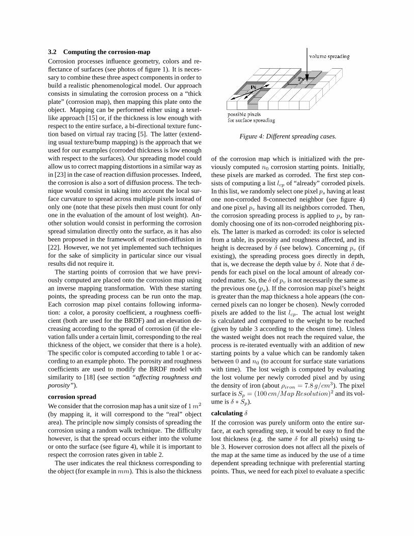
(by mapping it, it will correspond to the “real” objectarea). The principle now simply consists of spreading thecorrosion using a random walk technique. The difficultyhowever, is that the spread occurs either into the volumeor onto the surface (see figure 4), while it is important torespect the corrosion rates given in table 2.

The user indicates the real thickness corresponding tothe object (for example inmm). This is also the thickness

Figure 4: Different spreading cases.

of the corrosion map which is initialized with the pre-viously computedn0 corrosion starting points. Initially,these pixels are marked as corroded. The first step con-sists of computing a listlcp of “already” corroded pixels.In this list, we randomly select one pixelps having at leastone non-corroded 8-connected neighbor (see figure 4)and one pixelpv having all its neighbors corroded. Then,the corrosion spreading process is applied tops by ran-domly choosing one of its non-corroded neighboring pix-els. The latter is marked as corroded: its color is selectedfrom a table, its porosity and roughness affected, and itsheight is decreased byδ (see below). Concerningpv (ifexisting), the spreading process goes directly in depth,that is, we decrease the depth value byδ. Note thatδ de-pends for each pixel on the local amount of already cor-roded matter. So, theδ of pv is not necessarily the same asthe previous one (ps). If the corrosion map pixel’s heightis greater than the map thickness a hole appears (the con-cerned pixels can no longer be chosen). Newly corrodedpixels are added to the listlcp. The actual lost weightis calculated and compared to the weight to be reached(given by table 3 according to the chosen time). Unlessthe wasted weight does not reach the required value, theprocess is re-iterated eventually with an addition of newstarting points by a value which can be randomly takenbetween0 andn0 (to account for surface state variationswith time). The lost weigth is computed by evaluatingthe lost volume per newly corroded pixel and by usingthe density of iron (aboutρiron = 7.8 g/cm3). The pixelsurface isSp = (100 cm/MapResolution)2 and its vol-ume isδ ∗ Sp).

calculating δIf the corrosion was purely uniform onto the entire sur-face, at each spreading step, it would be easy to find thelost thickness (e.g. the sameδ for all pixels) using ta-ble 3. However corrosion does not affect all the pixels ofthe map at the same time as induced by the use of a timedependent spreading technique with preferential startingpoints. Thus, we need for each pixel to evaluate a specific

δ. This is achieved by calculating for each pixel a “localcorrosion time”tlocal : knowing the lost thickness of thispixel (this is the pixel height in the corrosion map), wecan calculate the equivalent lost weightweq:

weq = pixel heigth ∗ Sp ∗ ρiron

Solving equations of table 3 int leads to

tlocal = e(1/n)∗ln(weq/k)

The mean weight of matter to be lost at this time for thispixel is

∆w = w(tlocal + 1)− w(tlocal)

which corresponds to a mean height loss of

hl = ∆w/(ρiron ∗ Sp)

hl should correspond toδ, however a real surface can-not be handled in such a constant way as it might containimpurities or inclusions locally decreasing or increasingcorrosion rates. Since it is not actually possible to obtainall of this information, we empirically choose to add ran-domness by selectingδ as a random value aroundhl. Wenote that in the particular case of pitting corrosion,δ canbe increased by a physically defined factor called “pittingfactor” that is the ratio between the maximum depth of apit and the average thickness loss [17]. Since we did notdispose of experimental data concerning this value, weempirically used10 in our examples which gave visuallysatisfactory results.

Affecting roughness and porosity

On non-corroded parts, we use the Cook and TorranceBRDF model [3] for iron. On corroded parts, we use themodel described in [18] which accounts for both poros-ity and roughness. Porosity is empirically chosen to be80%, since rust is a very porous matter [17]. As de-scribed in [18], porosity increases the diffuse vs. spec-ular coefficients (indeed rust is not shiny as opposed toiron). Roughness was augmented by a factor of about3,which approximately corresponds to the values that wemeasured using a HommelWerke HommelTester T2000:a profile and roughness measurement tool (see figure 5).

Figure 6 illustrates the corrosion spread (changes ofcolor and geometry) using the previously described ran-dom walk algorithm with 5 starting points and for dif-ferent corrosion times, under medium corrosivity. Thethickness of the map is1.2mm. During the corrosionprocess new starting points have been randomly added.

Figure 5: Roughness measurements of a corroded part(top) and a non-corroded part (bottom) of the same sur-face. For both figures the scale is the same.

Figure 6: Full corrosion spread using our modified ran-dom walk (holes begin to appear up to 5 years)

4 Results

In this section, we illustrate some of the previously de-scribed corrosion forms. First a galvanic corrosion hasbeen computed: a screw on a more noble metallic rod.Our algorithm detects that the screw does corrode at anaccelerated rate. On the left-top of figure 7: corrosionstarts on the invisible parts of the screw and propagatespreferentially from the screw border to its center. A realphotograph of the same kind of scene is also provided(left-bottom part). The spreading is done under high cor-rosive atmosphere during 5 years. Another kind of pre-diction that we introduced in this paper is based on differ-ential aeration. On figure 7-right, a metallic pipe comesout of a wall. Oxygen cannot access to the parts of thispipe that are “into” the wall. Corrosion starts preferen-tially in the close neighborhood of the wall, and just intothe wall hole. To render this image we choose a mediumcorrosivity and show the result for a 8 years period.

On figure 8, corrosion greatly affects the geometry ofthe tool. See in particular its sharp edge and its shad-ows (conditions are a medium corrosivity during 25 yearswith 20 starting points).

Figure 7: Prediction of corrosion spreading - Galvaniccorrosion (left) - Differential aeration (right)

Figure 8: Affected geometry of a tool

Figure 9 shows the differences obtained between pit-ting (the first line of pictures) and uniform corrosion (thesecond line). On a same column of this figure, the amountof wasted matter is the same (due do identical corrosivityand time) but in the case of pitting corrosion the spreadprocess goes mainly into the object, thus greatly affectingthe object geometry (“holes” creation). The uniform cor-rosion spread is mainly a surface one. From left to right,time is 1, 5 and 10 years under very high corrosivity (in-dustrial marine environment for example). Pitting pointshave been randomly chosen onto the corroded surface.

Finally, figure 10 illustrates that corrosion can be at theorigin of great amounts of wasted matter. The left part isa real highly corroded wheelbarrow, the right part is acorresponding rendered image (conditions are a high cor-rosivity during 12 years with 20 starting points, thicknessof the metal sheet is4mm ).

5 Conclusions and Future Work

We have proposed a first phenomenological model ad-dressing the simulation and rendering corrosion (rust) ofmetals (especially steels), using an approach based on ex-perimental data. The model affects color, reflectance andgeometry. A first attempt of a physically based automaticprediction has also been proposed to localize the begin-ning of corrosion reactions. Though our model dependson many parameters (yet it is very simplified and thus is

Figure 9: Pitting corrosion (top) compared to uniformcorrosion (bottom)

not a fully physical model), they remain intuitive enoughto be used in computer graphics applications, allowingfor a good control of the aspect of corroded surfaces.However, the model is limited to the corrosion “attack”itself, while we have not considered other accompany-ing effects. Indeed, often also non-corroded parts are af-fected by time. Pollution adherence, rust transport andother stresses also create aspect variations (this explainthe wheelbarrow color differences on the figure 10). Itshould be possible to use the technique developed in [7]for transport simulation. The corrosion BRDF may alsobe improved in several ways: in our future works, weintend to take into account multiple layers as well as sub-surface scattering. Also, mechanical properties of ma-terials need to be studied in order to predict for exam-ple the fracture of rusty objects when corrosion has re-moved enough matter. This can lead us to a completetime dependent system to predict the appearance of en-tire scenes after several years under different atmosphericconditions.

References

[1] JF Blinn, “Light Reflection Functions for Simu-lation of Clouds and Dusty Surfaces”, ComputerGraphics 16(3), pp. 21-29, ACM SIGGRAPH,1982.

[2] WD Callister, “Materials Science and Engineering:An Introduction”, John Wiley and Sons Inc. New-York, 1994.

Figure 10: Comparison between a real photograph and arenderer image of a corroded wheelbarrow

[3] RL Cook, KE Torrance, “A Reflectance Model forComputer Graphics”,Computer Graphics15(3),pp. 307-316, ACM SIGGRAPH, 1981.

[4] CP Dillon, “Forms of Corrosion, Recognition andPrevention”, NACE International, Houston, 1982.

[5] JM Dischler, “Efficiently Rendering Macro Geo-metric Surface Structures with Bi-Directional Tex-ture Functions”,Eurographics Workshop on Ren-dering, pp. 169-180, Vienna, 1998.

[6] J Dorsey, P Hanrahan, “Modeling and Rendering ofMetallic Patinas”.Computer Graphicspp. 387-396,ACM SIGGRAPH, 1996.

[7] J Dorsey, H Pedersen, P. Hanrahan, Flow andChanges in Appearance.Computer Graphics, pp.411-420, ACM SIGGRAPH, 1996.

[8] J Dorsey, A Edelman, H Jensen, J Legakis, HPedersen, “Modeling and Rendering of WeatheredStone”, Computer Graphics, pp. 225-234, ACMSIGGRAPH, 1999.

[9] MG Fontana, “Corrosion Engineering”, McGrawHill, New-York, 1986.

[10] S Gobron, N Chiba, “3D Surface Cellular Automataand their Applications”,Journal of Visualizationand Computer Animation, (10), pp. 143-158, 1999.

[11] HP Hack, D Taylor, “Metals Handbook”, 9th Edi-tion, Vol 13, ASM Metals Park, 1987.

[12] S Hsu, T Wong, “Simulating Dust Accumulation”,IEEE Computer Graphics and Applications15(1),pp. 18-22, 1995.

[13] I Icart, P Arques, “A Physically-based BRDF Modelfor Multilayer Systems with Uncorrelated RoughBoundaries”,Eurographics Workshop on Rendering2000.

[14] ISO Norm 9223, “Corrosivity Classification”.

[15] JT Kajiya, TL Kay, “Rendering Fur with Three Di-mensional Texture”,Computer Graphics23(3), pp.271-280, ACM SIGGRAPH, 1989.

[16] G Kortum, “Reflectance Spectroscopy”, Springer-Verlag, New-York, 1969.

[17] D Landolt, “Corrosion, chimie de surface desmetaux”, Presses Polytechniques et UniversitairesRomandes, Alden Press, Oxford, 1993.

[18] S Merillou, JM Dischler, D Ghazanfarpour, “ABRDF Post-Process to Integrate Porosity on Ren-dered Surfaces”,IEEE Transaction on Vizualisationand Computer Graphics, vol 6(4) oct-dec 2000.

[19] S Merillou, JM Dischler, D Ghazanfarpour, “Sur-face Scratches, Measuring, Modeling and Render-ing”, The Visual Computer,vol 17(1), pp. 30-45,2001.

[20] G Miller, “Efficient algorithms for local and globalaccessibility shading”,Computer Graphics, pp.319-326, ACM SIGGRAPH 1994.

[21] WM Mullin, EJ Shumaker, GJ Tyler, “StochasticKinetics of Corrosion and Fractal Surface Evolu-tion”, Journal of Corrosion Science and Engineer-ing, (1)7, 1997.

[22] G Turk, “Generating Textures on Arbitrary Surfacesusing Reaction-Diffusion”,Computer Graphics, pp.289-298, ACM SIGGRAPH, 1991.

[23] A Witkin, M Kass, “Reaction-Diffusion Textures”,Computer Graphics, pp. 299-308, ACM SIG-GRAPH, 1991.

[24] TT Wong, WY Ng, PA Heng, “A Geometry Depen-dent Texture Generation Framework for SimulatingSurface Imperfections”,Eurographics Workshop onRendering, pp. 139-150, 1997.