cortical learning via prediction

JMLR: Workshop and Conference Proceedings vol 40:1–21, 2015

Cortical Learning via Prediction

Christos H. Papadimitriou [email protected]. Berkeley

Santosh S. Vempala [email protected]

Georgia Tech

AbstractWhat is the mechanism of learning in the brain? Despite breathtaking advances in neuroscience,and in machine learning, we do not seem close to an answer. Using Valiant’s neuronal model as afoundation, we introduce PJOIN (for “predictive join”), a primitive that combines association andprediction. We show that PJOIN can be implemented naturally in Valiant’s conservative, formalmodel of cortical computation. Using PJOIN — and almost nothing else — we give a simplealgorithm for unsupervised learning of arbitrary ensembles of binary patterns (solving an openproblem in Valiant’s work). This algorithm relies crucially on prediction, and entails significantdownward traffic (“feedback”) while parsing stimuli. Prediction and feedback are well-knownfeatures of neural cognition and, as far as we know, this is the first theoretical prediction of theiressential role in learning.Keywords: Cortical algorithms, neuroidal computation, unsupervised learning, prediction, predic-tive join (PJOIN)

1. Introduction

Human infants can do some amazing things, and so can computers, but there seems to be almostno intersection or direct connection between these two spheres of accomplishment. In ComputerScience, we model computation through algorithms and running times, but such modeling quicklyleads to intractability even when applied to tasks that are very easy for humans. The algorithms weinvent are clever, complex and sophisticated, and yet they work in fashions that seem completelyincompatible with our understanding of the ways in which the brain must actually work — and thisincludes learning algorithms. Accelerating advances in neuroscience have expanded tremendouslyour understanding of the brain, its neurons and their synapses, mechanisms, and connections, andyet no overarching theory appears to be emerging of brain function and the genesis of the mind. Asfar as we know, and the spectacular successes of neural networks (Hinton and Salakhutdinov, 2006;LeCun et al., 1998) notwithstanding, no algorithm has been proposed which solves a nontrivialcomputational problem in a computational fashion and style that can be plausibly claimed to reflectwhat is happening in the brain when the same problem is solved. This is the scientific context ofour work.

We believe that formal computational models can play a valuable role in bridging these gaps.We have been inspired in this regard by the pioneering work of Les Valiant on the neuroidal model, arandom directed graph whose nodes and edges are capable of some very local computation (Valiant,1994). We have also been prompted and influenced by certain interesting facts and conjecturesabout the brain’s operation, which have been emerging in recent years. First, even though the

c© 2015 C.H. Papadimitriou & S.S. Vempala.

PAPADIMITRIOU VEMPALA

visual cortex, for example, processes sensory input in a hierarchical way, proceeding from areaslower in the hierarchy to higher areas (from retina to LGN and V1, from there to V2, to V4, toMT, etc.), there seem to be many neuronal connections, and presumably significant firing traffic,directed downwards in this hierarchy (see e.g., (Lamme and Roelfaema) and subsequent work);this is usually referred to as “feedback.” Second, there seems to be an emerging consensus amongstudents of the brain that prediction may be an important mode of brain function (Churchland et al.,1994; Hawkins and Blakeslee, 2004; Rao and Ballard, 1999): For example, vision involves not justpassive hierarchical processing of visual input, but also active acquisition of new input via saccades(rapid forays to new parts of the visual field), whose purpose seems to be to verify predictions madeby higher layers of the visual cortex; significantly, many eye muscles are controlled by low areasof the visual hierarchy. Third, the connections in the cortex seem to deviate from the standard Gnp

model of random graphs (Erdos and Renyi, 1960), in that reciprocal connections (closing cycles oflength two) and transitive connections (connecting nodes between which there is a path of lengthtwo ignoring directions) are much more likely than Gnp would predict (Song et al., 2005).

Valiant models the cortex as a random directed graph of neuroids (abstract neuron-like ele-ments) connected via directed edges called synapses. The algorithms running on this platform arevicinal, by which it is meant that they are local in a very strict sense: the only communication fromother neuroids that a neuroid is allowed to receive is the sum of the action potentials of all currentlyfiring neuroids with synapses to it. An important further consideration in the design of vicinal algo-rithms is that there should be minimal global control or synchronization needed during its execution.Valiant goes on to posit that real-world objects or concepts can be represented by sets of neuroids.There is a long tradition of using such sets of neurons, or equivalently sparse binary vectors, as thebasic unit of brain function, see e.g. Kanerva (1988). In our reading, Valiant’s model is the mostexplicitly algorithmic such framework. If one assumes that the underlying directed graph is randomin the sense ofGnp, and taking into account what is known from neuroscience, Valiant (1994, 2005)argues carefully that it is possible to choose some number r, perhaps between 10 and 100, such thatsets of r neurons can usefully represent a concept. Such sets are called items, and they constitutethe basic element of Valiant’s theory: all r neuroids of an item firing (or perhaps some overwhelm-ing majority thereof) is coterminal with the corresponding concept being “thought about.” Valiantshows that such items can be combined through the basic operations of JOIN and LINK, creatingcompound new items from, respectively simply connecting, existing items. For example, if A andB are items (established sets of about r neuroids) then Valiant shows how to create, via a vicinalalgorithm, a new item JOIN(A,B) which stands for the combination, or conjunction, of the twoconstituent items (see also Feldman and Valiant (2009)). A major open problem in Valiant’s workis hierarchical memorization for patterns with more than two items.

Our main contribution is two-fold: the formulation and implementation of a new operation onitems that we call predictive join or PJOIN, and its application to a vicinal algorithm with minimalcontrol for the hierarchical memorization of arbitrary length patterns. PJOIN extends JOIN in that, ifonly one of the constituent elements of PJOIN(A,B) fires, sayA fires, then the structure will predictB, and initiate a sequence of downstream events whose purpose is to check this prediction. Weshow (Theorem 1) that the PJOIN of two items — which may be, and typically will be, themselvesPJOINs — can be created by a vicinal algorithm so that it functions according to certain precisespecifications, capturing the discussion above. We do not know how to implement PJOIN usingonly the existing primitives of JOIN and LINK.

2

CORTICAL LEARNING VIA PREDICTION

We suspect that the power of cortical computation lies not so much in the variety and sophis-tication of the algorithms that are actually implemented in cortex — which might be very limited— but in the massive scale of cortex and the ways in which it interacts with an appropriately inter-esting environment through sensors and actuators; cortical architecture may happen to be very welladapted to the kinds of environments mammals live in. Here we use our PJOIN operation — andalmost nothing else — to design a spontaneous vicinal algorithm, i.e., with minimal global control,for performing a basic task that would be required in any such interaction with an environment:unsupervised learning of a set of patterns. By learning we mean that, if a pattern is presented to asensory device for long enough, then our vicinal algorithm will “memorize it,” in that it will createa structure of items connected by PJOINs which represent this pattern. If many patterns are pre-sented, one after the other, all these patterns will be memorized in a shared structure. If sometimein the future one of the already presented patterns is presented again, then with high probability thestructure will “recognize it,” by which we mean that there will be one special item (set of neuroids)whose firing will signal the act of recognition of that particular item. It is rather immediate thatsuch performance would be impossible to achieve through JOIN alone; our work can be viewed asa blackbox reduction of learning n-length patterns to the primitive binary operations of PJOIN. Theproperties of our learning algorithm are stated as our Theorem 2. Its proof (in Appendix P) boundsthe depth of the PJOIN structure created, as well as the number of rounds of pattern presentationsafter which the top-level item for a pattern becomes stable. These bounds are not a priori obvious,as interleaved presentations of multiple patterns can lead to the creation of new PJOINs and new“recognition pathways” for familiar patterns. Nevertheless we show that, for any set of patterns andany order of presentation, the resulting memory structures are efficient and stable. Moreover, usingonly JOIN/LINK does not suffice for even a single pattern of size n > 2 as it leads to combinato-rial explosion of JOINs. Instead, PJOIN solves this problem (for any number of patterns) throughprediction and sharing — two much observed functions in psychology and neuroscience, of whichwe may be providing the first rigorous support. We remark that classical Hopfield networks forassociative memories (Hopfield, 1982) are a non-vicinal solution to a different problem.

In Section 5 we discuss several important issues surrounding our results. We simulated thesealgorithms and measured their performance on binary patterns, including the sizes of representa-tions created and updates to them, the total traffic generated in each presentation, and the fraction oftraffic that is downward. The results, summarized in Section 6, are consistent with our theoreticalpredictions. In particular, both memorization and recognition of patterns of 100 bits are accom-plished in a rather small number of “parallel steps” — firings of individual neuroids — typically inthe low tens; this is an important desideratum, since complex cognitive operations can be performedin less than second, and thus in fewer than a hundred steps. In Section 7, we outline further stepsfor this research program.

2. Valiant’s Computational Model of Cortex

The basic structure in Valiant’s computational theory of cortex is an item, which represents in thebrain a real-world element, object, or concept. Each item is implemented as a set of neurons. Valiantconsiders two alternative representations, one in which these sets are disjoint and one in which theymay overlap; here we shall work in the disjoint framework, but we see no reason why our work couldnot be extended to overlapping items. Once such a set of neurons has been defined, the simultaneous

3


firing of these neurons (or perhaps of some “overwhelming majority” of them) represents a brainevent involving this item.

Valiant defines two key operations involving items. The JOIN operation creates, given two itemsA andB, a new item C = JOIN(A,B). Once the new item has been created, every time bothA andB fire, C will fire in the next instant. A second operation is LINK. Given two established items Aand B, the execution of LINK(A,B) has the effect that, henceforth, whenever item A fires, B willfire next.

Vicinal algorithms. Valiant showed that the operations of JOINand LINK— both the creation ofthese capabilities, and their application — can be implemented in a minimalistic model of compu-tation by neurons that he called vicinal algorithms.

The substrate of vicinal algorithms is a directed graph whose vertices are neuroids, (idealizedneurons) connected through directed edges called synapses. At every discrete time t ≥ 0, a neuroidvi is at a state (T t

i , fti , q

ti) consisting of three components: a positive real number T t

i called itsthreshold; a Boolean f ti denoting whether i is firing presently; and another memory qti which cantake finitely many values. In our algorithms, T will for the most part be kept constant. Similarly,every synapse eji from neuroid vj to neuroid vi has a state (wt

ji, qqtji) consisting of a real number

wtji called its strength; plus another finitary memory qqtji. When the superscript t is understood

from context, it will be omitted.The operation of vicinal algorithms is strictly local: neuroids and synapses update their own

state in discrete time steps. The only way that the operation of neuroid vi can be influenced by otherneuroids is through the quantity Wi =

∑j:fj=1wji, the sum total of incoming action potentials. At

each time instant, the firing status of all neuroids is updated:

W ti ←

∑j:f t

j=1

wtji; if W t

i ≥ T ti then f

t+1i ← 1,

and after that the remaining of the state of the neuroids, and the state of the synapses, are updated:

(T t+1i , qt+1

i )← δ(T ti , q

ti , f

t+1i ,W t

i ),

(wt+1ji , qqt+1

ji )← λ(qti , qqtji, f

tj , f

t+1i ,W t

i ).

That is, at each step fi is set first — this is tantamount to assuming that the action potentials ofother neuroids are transmitted instantaneously — and then the remaining state components of theneuron’s state, and also of its incoming synapses, are updated in an arbitrary way. Notice that theupdate functions δ and λ are the same for all neuroids vi and synapses eji.

It is argued by Valiant (2000, 2006) that vicinal algorithms realistically (if anything, conserva-tively) capture the capabilities of neurons. Furthermore, it is also argued (Valiant, 2005, 2012) thateven cascading usage of these two operations (taking the JOIN of two JOINs, and then again, and soon) is up to a point a reasonably realistic hypothesis. Valiant (2005) presented two particular vicinalalgorithms which create, given two items A and B, create the item C = JOIN(A,B), or LINK A toB. For the interested reader, we explain these two algorithms in Appendix A.

Refraction. Neurons in the brain are known to typically enter, after firing, a refractory periodduring which new firing is inhibited. In our model, the firing of a neuroid can be followed by arefractory period of R steps. This can be achieved through R memory states, say by increasing the

4


neuroid’s threshold T by a factor of 2R−1, and subsequently halving it at every step. We shall rou-tinely assume that, unless otherwise stated, the firing of an item will be followed by one refractorystep.

3. Predictive JOIN

We now propose an enhanced variation of JOIN, which we call predictive JOIN, or PJOIN(A,B).As before, every time A and B fire simultaneously, C will also fire. In addition, if only A fires,then C will enter a state in which it will “predict B,” in which C will be ready to fire if just B fires.Similarly, a firing of B alone results in the prediction of A. The effect is that the firing of A and Bnow need not be simultaneous for C to fire.

But there is more. Having predicted B, C will initiate a process whereby its prediction ischecked: Informally, C will “mobilize” a part of B. If B also happens to be the predictive JOIN ofsome items D and E, say (as it will be in the intended use of PJOIN explained in the next section),then parts of those items will be mobilized as well, and so on. A whole set of items reachable fromB in this way (by what we call downward firings) will thus be searched to test the prediction. As weshall see in the next section, this variant of JOIN can be used to perform some elementary patternlearning tasks.

Implementation of PJOIN. The vicinal algorithm for creating PJOIN(A,B) is the following:

Create PJOIN(A,B)

1. First, create C = JOIN(A,B), by executing the two-step vicinal algorithm mentioned aboveand described in the Appendix.

2. Each neuroid in C participates in the next steps with probability half. Valiant (2000) allowsvicinal algorithms to execute randomized steps, but here something much simpler is required,as the random bit needed by a neuroid could be a part of that neuroid, perhaps depending onsome component of its identity, such as its layer in cortex. We shall think of the chosen half(in expectation) of the neuroids of item C as comprising a new item which we call CP , for“predictive C.” That is, the neurons of item CP are a subset of those of item C. (Strictlyspeaking this is departure from Valiant’s disjoint model of implementing items, but it is avery inessential one.) The neuroids of C that are not in CP now enter a total state calledOPERATIONAL, ready to receive firings from A and/or B as any neuroid of JOIN(A,B)would.

3. Suppose now that A and B are predictive joins as well, and therefore they have parts AP andBP (this is the context in which PJOIN will be used in the next section). In the next twosteps we perform LINK(CP , AP ) and LINK(CP , BP ), linking the predictive part of C tothe predictive parts of its constituent items; there is no reason why the two LINK operationscannot be carried out in parallel. In the discussion section we explain that this step can besimplified considerably, omitting the LINK operations, by taking into account certain knownfacts about the brain’s connectivity, namely the reciprocity of synapses. After these LINKcreations, the working synapses from the relay neuroids to the neuroids of AP and BP willbe in a memory state PARENT identifying them as coming “from above.” Such synapseswill have a strength larger than the minimum required one (say, double), to help the neuronsidentify firings from a parent.

5


4. After this is done, CP enters the total state P-OPERATIONAL, where all strengths of synapsesfrom A and B to CP (but not to the rest of C) are doubled. The effect is that the neuroids ofCP will fire if eitherA fires, orB fires, or both. This concludes the creation of PJOIN(A,B).Notice that it takes four steps (we discuss in the last section one possible way to simplify it tothree steps). After the creation of the predictive join is complete, indeed, if only one of A orB fires, then CP will fire, initiating a breadth-first search for the missing item.

To summarize, we show below the vicinal algorithm, which we call Create PJOIN(A,B):

Steps 1 and 2 C = JOIN(A,B);

After Step 2 CP consists of about half of the neurons in C. C and not CP ⇒OPERATIONAL

Steps 3 and 4 LINK(CP , AP );LINK(CP , BP )

After Step 4 AP , BP ⇒ L-OPERATIONAL synapses in PARENT memory state;CP ⇒ P-OPERATIONAL (synapses fromA,B double their strength).

The operation of PJOIN(A,B) is as follows (it is a more elaborate version of that of JOIN,explained in the Appendix):

1. If both inputs A and B fire simultaneously, then PJOIN(A,B) will operate as an ordinaryJOIN.

2. As soon as one of A and B fires — suppose that A fires — then CP fires (because of thedoubled synaptic strengths), an event that will cause BP to fire downwards in the next step.Notice that AP will not fire as a result of CP firing, because it is in a refractory state. Also,after the firing of A, the neuroids in C double the strength of the synapses coming from B(that is, from neuroids that do not come from a parent and are refractory), and all of C entersa total state called PREDICTING B. Thus, if henceforth the predicted item B fires, all of Cwill fire.

3. CP ’s firing will cause BP to fire downwards in the next step; AP does not fire as a resultof CP firing, because it is in a refractory state. After this, CP enters a PASSIVE total state,in which it will ignore firings of the EP part of any item E = PJOIN(C,D) further above.Again, this is accomplished by setting the strength of these synapses (which are the ones inthe PARENT memory state) to zero.

4. If henceforth the predicted item B fires, then C fires and all of A,B,C go back to the OPER-ATIONAL (P-OPERATIONAL for CP ) total state.

5. Finally, if one of C’s parents (by which we mean any item of the form PJOIN(C,D)) fires“downwards,” then the neurons inCP will fire (we think of them as firing “downwards”), thuspropagating the search for the predicted items.

The state diagram of the desired operation of PJOIN(A,B) is shown in Fig. 1.

Theorem 1 There is a vicinal algorithm that creates in four steps an item PJOIN(A,B) operatingas specified by the diagram in Figure 1.

For the proof see Appendix P.

6


Figure 1: The operational state transition diagram for an item created by PJOIN

Remark: Control and Synchrony. Vicinal algorithms should run with minimum control andsynchrony. By control we mean firings initiated by outside events, other than the firing of neuroidsexplicitly mentioned in the algorithm. The only control needed in our vicinal algorithms so far isthe initiation of the firings of A and B, in consecutive steps, during the creation of JOIN(A,B). InSection 5 we shall discuss briefly how all control necessary for vicinal algorithms can actually beimplemented vicinally.

Similarly, expecting billions of neurons to operate in precise lockstep is not realistic, and sovicinal algorithms should not require much synchrony. The only synchronization needed in ouralgorithms, besides the synchronous firing of all neurons of an item in response to the neurons ofanother item firing (a necessary assumption for Valiant’s model, and whose plausibility we discussin Section 5), is between the firing of two items in the two steps of the creation of JOIN(A,B) andthe two steps of LINK(A,B) (and we shall soon argue that the latter one may not be necessary).

4. Unsupervised Learning

Cortical activity acquires meaning only when it interacts with the world via appropriate sensors andactuators. In this section we show that the primitive PJOIN enables a neurally plausible algorithmfor memorizing and recognizing patterns.

Sensing the environment. By pattern we mean a binary vector with n coordinates, that is, amember of {0, 1}n for some parameter n (visual patterns are only one of the many possibilities).Note that the binary nature of the input is for conceptual convenience alone, multi-valued inputs canbe accommodated easily. In particular, we shall assume that there are n special items S1, . . . , Sncalled sensors. Each Si has two special memory states, ZERO and ONE, so that the memory statesof all n sensors “spell” the pattern. Importantly, geometry is absent from our model and algorithm,in that it is oblivious of the order of the sensors. Associated with each sensor Si there are two otheritems which we denote by 0i and 1i, such that:

• The states of the n sensors will remain unchanged during a period that we call pattern pre-sentation. During such presentation, each sensor fires at most one — either spontaneously ata random time, or when predicted.

7


• The only activity of the neuroids of sensor Si is the aforementioned firing, as well as theoccasional change in memory state when a different pattern is presented.

The memory states of the n sensors typically remain unchanged from one time step to the next,displaying a pattern x ∈ {0, 1}n. A maximum time period during which these memory statesare unchanged is called a presentation of the corresponding pattern. We assume that, during sucha presentation, the n sensor items fire spontaneously at random, each at most once. After thepresentation of one pattern concludes, the presentation of a different pattern begins, and so on.

Memorization and recognition. We say that pattern x ∈ {0, 1}n has been memorized if, duringits first presentation, a hierarchical structure of items is eventually formed with one top item I(x)(that is, an item that does not participate in further PJOINs) which we think of as “representing”the presented pattern, in that, if x and y are different patterns, I(x) 6= I(y). Notice that x’s firstpresentation may follow the presentation of many other patterns y, z, w . . ., and so its memorizationstructure will be “built” on top of existing memorization structures of the other patterns. Now if, inany subsequent presentation of the same pattern x, this special item I(x) fires and is the highest-level item that fires, we say that the pattern has been recognized.

Learning with PJOIN. Before describing the algorithm for learning, we make a few remarks onsensor items:

1. If sensor Si fires in state ONE, item 1i fires next; similarly, if it fires in state ZERO,, 0i fires. Thiscan be achieved, for example, by LINKing Si to both 0i and 1i, and appropriately manipulating thestrengths of the corresponding synapses according to the memory state (ZERO or ONE) of Si.

2. The items 0i and 1i participate in PJOINs with other items, and thus they form the“basis” of thePJOIN structure which will be eventually formed in response to the current pattern presentation. By“basis” we mean that these are the only items in the structure that are not themselves PJOINs ofother items (see Figure 2).

3. There is one difference between these basis items and the other PJOIN items in the structure:As we have seen, if C = PJOIN(A,B) then its predictive part, CP , synapses to AP and BP . Incontrast, if C = 1i or 0i then CP synapses to the corresponding Si item. Thus, every time 1i or 0i“fires downwards” Si fires next, completing the chain of predictions. Importantly, it does so withoutrefraction (because it may have to fire in the next step to verify the prediction).

4. If and when a sensor item is predicted by a parent PJOIN, its sampling weight is increased,multiplied by a factor M > 1.

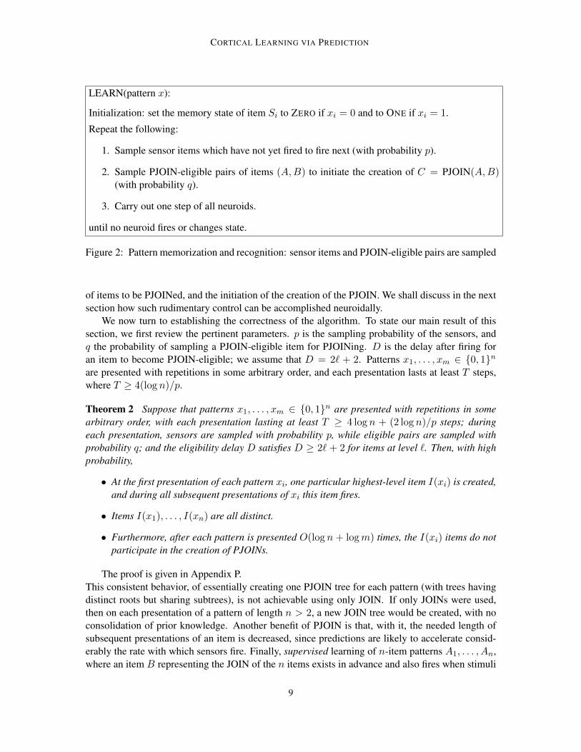
Learning is achieved by the algorithm shown in Figure 2. We say that an item is PJOIN-eligibleif at least D time steps have elapsed after it has fired, and none of its parents has fired for the pastD steps, where D > 0 is a parameter. Define the level of an item to be zero if it is an item ofthe form 0i or 1i; and otherwise, if it is PJOIN(A,B), to be one plus (recursively) the largest ofthe levels of A and B. In our algorithm, we allow the delay D associated with an item to dependon the level of the item. The selection of pairs to be PJOINed is as follows: PJOIN-eligible itemsare sampled, each with probability q. Note that, even though the algorithm of Figure 2 is depictedas running synchronously, the only synchrony that is necessary for its correctness is between theneuroids of the same item, and between pairs of items being joined. Furthermore, the only control(firings of neuroids initiated by events outside the algorithm, that is, by events other than firings ofother neuroids), is the spontaneous firing of sensor items and the selection of PJOIN-eligible pairs

8


LEARN(pattern x):

Initialization: set the memory state of item Si to ZERO if xi = 0 and to ONE if xi = 1.

Repeat the following:

1. Sample sensor items which have not yet fired to fire next (with probability p).

2. Sample PJOIN-eligible pairs of items (A,B) to initiate the creation of C = PJOIN(A,B)(with probability q).

3. Carry out one step of all neuroids.

until no neuroid fires or changes state.

Figure 2: Pattern memorization and recognition: sensor items and PJOIN-eligible pairs are sampled

of items to be PJOINed, and the initiation of the creation of the PJOIN. We shall discuss in the nextsection how such rudimentary control can be accomplished neuroidally.

We now turn to establishing the correctness of the algorithm. To state our main result of thissection, we first review the pertinent parameters. p is the sampling probability of the sensors, andq the probability of sampling a PJOIN-eligible item for PJOINing. D is the delay after firing foran item to become PJOIN-eligible; we assume that D = 2` + 2. Patterns x1, . . . , xm ∈ {0, 1}nare presented with repetitions in some arbitrary order, and each presentation lasts at least T steps,where T ≥ 4(log n)/p.

Theorem 2 Suppose that patterns x1, . . . , xm ∈ {0, 1}n are presented with repetitions in somearbitrary order, with each presentation lasting at least T ≥ 4 log n + (2 log n)/p steps; duringeach presentation, sensors are sampled with probability p, while eligible pairs are sampled withprobability q; and the eligibility delay D satisfies D ≥ 2` + 2 for items at level `. Then, with highprobability,

• At the first presentation of each pattern xi, one particular highest-level item I(xi) is created,and during all subsequent presentations of xi this item fires.

• Items I(x1), . . . , I(xn) are all distinct.

• Furthermore, after each pattern is presented O(log n + logm) times, the I(xi) items do notparticipate in the creation of PJOINs.

The proof is given in Appendix P.This consistent behavior, of essentially creating one PJOIN tree for each pattern (with trees havingdistinct roots but sharing subtrees), is not achievable using only JOIN. If only JOINs were used,then on each presentation of a pattern of length n > 2, a new JOIN tree would be created, with noconsolidation of prior knowledge. Another benefit of PJOIN is that, with it, the needed length ofsubsequent presentations of an item is decreased, since predictions are likely to accelerate consid-erably the rate with which sensors fire. Finally, supervised learning of n-item patterns A1, . . . , An,where an item B representing the JOIN of the n items exists in advance and also fires when stimuli

9


are presented, can be reduced to unsupervised learning as follows: the above algorithm creates anitem C = PJOIN(A1, . . . , An). Following that, we perform LINK(C,B) and LINK (B,C), so that Bfires whenever C does and vice versa.

5. Some Remarks on Control

Vicinal algorithms are intended to be an austere, and therefore realistic, model of computation bythe neurons in cortex. And yet certain aspects of the way we are using vicinal algorithms in thiswork require some further discussion and justification.

Perhaps the most striking aspect of the use of vicinal algorithms on items, as pioneered byValiant, is the assumption that the r neuroids of an item can fire in synchrony, for example toinitiate the creation of a JOIN or a PJOIN. We refer to this extraneous ability as “control.” Inthe current section we briefly discuss how such control could be plausibly implemented within thevicinal model.

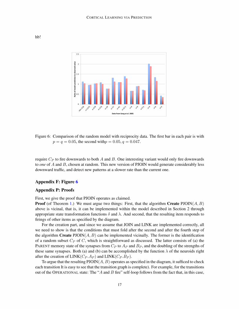
Reciprocity and a modified random graph model. Valiant’s basic model assumes that neuroidsare connected by a random directed graph of synapses in the Gnp model in which all possible edgeshave the same probability p of being present. Measurements of the cortex, however, suggest amore involved model. In particular, Song et al. (2005) and subsequent work show that synapticreciprocity (the chance that there is an edge from i to j and from j to i) is far greater than random.This is established for pairs chosen from quadruple whole-cell recordings, where the cells tend tobe within close proximity of each other. The same is true of synaptic transitivity, i.e., the chancethat two nodes connected by a path of length 2 are also connected directly.

A simple extension of the classical Gn,p random graph model can account reasonably well forthese departures from randomness. We propose the following: We start with n vertices. For everypair of vertices i, j within a distance threshold (in the case of the data from Song et al. (2005), thisapplies to every pair), with probability p only the i→ j edge is in the graph; with probability p onlyj → i; and with probability q both are in the graph; we assume that 2p+ q < 1. With the remaining1− (2p+ q) probability, no arc exists between i and j.

This is already a useful model, incorporating the apparent reciprocity of cortical connections.A more elaborate two-round model also introduces transitivity. The first round is as above. In thesecond round, for each pair i, j with no arc between i and j, for every other proximal vertex k, ifthere is a path of length two between i and j from the first round, ignoring direction, then we addi → j with probability r · p/(2p + q), same for j → i, and we add both arcs with probabilityr · q/(2p+ q). This two-round model, with the specific values of p = 0.05, q = 0.047 and r = 0.15gives a reasonable fit with the data in Song et al. (2005) (see Figure 6 in the Appendix).

An alternative implementation of PJOIN(A,B) Once we assume that the neuroids have richreciprocal connections between them, many possibilities arise. For a first example, the creation ofPJOIN(A,B) can be simplified a little. After the neuroids of C have been chosen, CP could consistof all neuroids in C which happen to have reciprocal connections back to AP and BP . Now theLINK step is unnecessary, and the creation of a PJOIN can be carried out in three steps, as opposedto four.

Using reciprocity for control. Consider an item A. Is there a neuroid which is connected to eachof the r neuroids through a path of reciprocal connections of the same small length, call it `? Forreasonable values of n (total number of available neuroids, say 109), r (number of neuroids in an

10


item, say 50-100), and q (probability that two neuroids are connected in both directions, say 10−5)it is not hard to see that such a neuroid is very likely to exist, with ` is bounded by

r − 1

r· log nlog qn

≤ 3.

Furthermore, we can suppose that such a neuroidRA (“the root of itemA”) is discovered by a vicinalprocess soon after the establishment of item A. One can then imagine that, once the neuroids ofA fire, their root can sense this, and make them fire synchronously in a future step, to create aPJOIN(A,B), as required by our algorithm. The delay parameter D of our memorization algorithmmay now be seen as the required number of steps for this synchronization to be set up.

Simultaneous PJOINs. Another important step of our memorization algorithm, whose imple-mentation in cortex may seem problematic, is the selection of items to be PJOINed. How are theyselected, and how are they matched in pairs? And, furthermore, won’t the POISED neuroids (re-call the creation of a JOIN described in Section 2) be “confused” by all other items firing at once?Valiant’s algorithm for creating JOINs assumes implicitly that nothing else is happening duringthese two steps; the simultaneous creation of several JOINs requires some thought and explanation.

Suppose that several PJOIN-eligible items fire, presumably in response to control signal fromtheir respective roots, as hypothesized earlier. It is reasonable to assume that these firings are notsimultaneous, but occur at times differing by a fraction of the duration of a step. One step afterthe first firing of an item A, and in response to that firing, several neuroids are POISED to becomepart of a PJOIN of A with another item. If we represent the firing of item A just by the symbol A,and the time of first availability of the POISED items for it as A′, a sequence of events during ourmemorization algorithm can look like this:

. . . A, B, C, A′, D, B′, C ′, E, F, D′, G . . .

whereA′ happens one step afterA and similarly forB′ afterB, etc. Now this sequence of events willresult in the following PJOINs being formed: PJOIN(A,D), PJOIN(B,E), PJOIN(C,E),PJOIN(D,G).Notice thatE formed two PJOINs, with bothB andC, and F formed none, and this is of course fine.This way, the spontaneous formation of PJOINs envisioned by our algorithm can happen withoutundesired “interference” between different PJOINing pairs, and with only minimal control.

We believe that this alternative way to select items to be PJOINed in our learning algorithm (bychoosing random stars joining existing items, instead of random edges) enjoys the same favorablequantitative performance properties established by Theorem 2.

6. Experiments (summary)

We implemented our unsupervised learning algorithm to check its correctness, but also to gauge itstrue performance. For patterns of 100 bits, presentations lasted for about 15 to 40 steps. A largefraction of the traffic (typically between 30% and 55%) was indeed downwards, and much overlapin PJOINs between patterns was noted. The creation of new PJOINs in repeated presentations ofthe same pattern was very limited. For details of the experiments, and charts, see Appendix E.

7. Conclusion and further work

We have introduced a new primitive, PJOIN, intended to capture the combining and predicting ac-tivity apparently taking place in cortex, and which can be implemented in Valiant’s minimalistic

11


model of vicinal algorithms. We showed that, by allowing items to spontaneously form PJOINs,starting from sensory inputs, complex patterns can be memorized and later recognized within veryreasonable time bounds. Much of the activity in this pattern recognition process consists of predict-ing unseen parts of the pattern, and is directed “downwards” in the hierarchy implied by PJOINs, inagreement with current understanding.

This work touches on the world’s most challenging scientific problem, so there is certainly nodearth of momentous questions lying ahead. Here we only point to a few of them that we see asbeing close to the nature and spirit of this work.

Invariance. We showed how PJOINs can be a part of the solution of a rather low-level problemin cognition, namely the memorization and recognition of patterns. Naturally, there are much morechallenging cognitive tasks one could consider, and we discuss here a next step that is both naturaland ambitious. One of the most impressive things our brain seems to accomplish is the creation ofinvariants, higher-level items capturing the fact that all the various views of the same object fromdifferent angles and in different contexts (but also, at an even higher level, all sounds associatedwith that object or person, or even all references to it in language, etc.), all refer to one and the samething. It would be remarkable if there is simple and plausible machinery, analogous to PJOIN, thatcan accomplish this seemingly miraculous clustering operation.

Language. Language and grammar seem to us to be important challenges that are related to theproblem of invariance, and in fact may be central to a conceptual understanding of brain function.Language may be a “last-minute” adaptation, having arrived at a time (possibly 50,000 years ago)when human cortex was fully developed. One can conjecture that language evolved by taking fulladvantage of the structure and strengths of cortex, and hence can give us clues about this structure.

A PJOIN machine? This work, besides introducing a useful cortical primitive, can be also seenas a particular stance on cortical computation: Can it be that the amazing accomplishments ofthe brain can be traced to some very simple and algorithmically unsophisticated primitives, whichhowever take place at a huge scale? And is there a formal sense in which prediction and feedbackare necessary ingredients of efficient cognition by cortex?

Modeling the environment. If indeed cortical computation relies not on sophisticated algorithmsbut on crude primitives like PJOIN, then the reasons for its success must be sought elsewhere,and most probably in two things: First, the environment within which the mammalian cortex hasaccomplished so much. And secondly, the rich interfaces with this environment, through sensorsand actuators and lower-level neural circuits, resulting, among other things, in complex feedbackloops, and eventually modifications of the environment. What seems to be needed here is a newtheory of probabilistic models capable of characterizing the kinds of “organic” environments ap-pearing around us, which can result — through interactions with simple machinery, and presumablythrough evolution — to an ascending spiral of complexity in cognitive behavior.

Acknowledgements. We are grateful to Tatiana Emmanouil and Sebastian Seung for useful ref-erences, and to Vitaly Feldman and Les Valiant for helpful feedback on an earlier version of thispaper. This research was supported by NSF awards CCF-0964033, CCF-1408635, CCF-1217793and EAGER-1415498, and by Templeton Foundation grant 3966.

12


References

Patricia S. Churchland, V. S. Ramachandran, and Terrence J. Sejnowski. A critique of pure vision.In Cristof Koch and Joel L. Davis, editors, Large Scale Neuronal Theories of the Brain. MITPress, Cambridge, MA, 1994.

Paul Erdos and Alfred Renyi. On the evolution of random graphs. Publ. Math. Inst. Hungary. Acad.Sci., 5:17–61, 1960.

Vitaly Feldman and Leslie G. Valiant. Experience-induced neural circuits that achieve high capacity.Neural Computation, 21(10):2715–2754, 2009. doi: 10.1162/neco.2009.08-08-851.

Jeff Hawkins and Sandra Blakeslee. On Intelligence. Times Books, 2004. ISBN 0805074562.

G E Hinton and R R Salakhutdinov. Reducing the dimensionality of data with neural networks.Science, 313(5786):504–507, July 2006.

J. J. Hopfield. Neural networks and physical systems with emergent collective computational abil-ities. Proceedings of the National Academy of Sciences of the United States of America, 79(8):2554–2558, 1982.

P. Kanerva. Sparse Distributed Memory. A Bradford book. MIT Press, 1988. ISBN9780262111324. URL http://books.google.com/books?id=I9tCr21-s-AC.

Victor A. F. Lamme and Pieter R. Roelfaema. Trends in Neurosciences, page 571.

Yann LeCun, Lon Bottou, Yoshua Bengio, and Patrick Haffner. Gradient-based learning applied todocument recognition. In Proceedings of the IEEE, volume 86, pages 2278–2324, 1998.

R.P.N. Rao and D.H. Ballard. Predictive coding in the visual cortex: a functional interpretation ofsome extra-classical receptive-field effects. Nature Neuroscience, 2:79–87, 1999.

S Song, PJ Sjostrom, M Reigl, S Nelson, and DB Chklovskii. Highly nonrandom features ofsynaptic connectivity in local cortical circuits. PLoS Biology, 3(3), 2005.

Leslie G. Valiant. Circuits of the mind. Oxford University Press, 1994. ISBN 978-0-19-508926-4.

Leslie G. Valiant. A neuroidal architecture for cognitive computation. J. ACM, 47(5):854–882,2000. doi: 10.1145/355483.355486.

Leslie G. Valiant. Memorization and association on a realistic neural model. Neural Computation,17(3):527–555, 2005. doi: 10.1162/0899766053019890.

Leslie G. Valiant. A quantitative theory of neural computation. Biological Cybernetics, 95(3):205–211, 2006. doi: 10.1007/s00422-006-0079-3.

Leslie G. Valiant. The hippocampus as a stable memory allocator for cortex. Neural Computation,24(11):2873–2899, 2012. doi: 10.1162/NECO a 00357.

13

http://books.google.com/books?id=I9tCr21-s-AC


Appendix A: The JOIN and LINK Operations

Given two items A and B, each represented by r neuroids, the operation JOIN(A,B) can be imple-mented in two steps, as follows:

• The neuroids that will represent C = JOIN(A,B) will be recruited from a population ofneuroids such that there are expected (on the basis of the random graph properties of theneuroidal network) to exist at least k synapses going from each of A,B to at least r of theseneuroids, for some desired parameters r, k. These neuroids are initialtly at a total state thatwe call CANDIDATE: not firing, all memories at some null state, the standard threshold T ,and all strengths of incoming synapses equal to T

k .

• At the first step, all neuroids in A fire. If, at the end of this step, a candidate neuroid fires (andtherefore it had at least k synapses coming from A), then its total state becomes one that wecall POISED: all synapses that come from firing A neuroids have now strength T 2

2kWi(so that

if all neuroids of A fire again, they will together achieve a sum of T2 ; recall thatWi is the total

strength of all synapses from A, and therefore kWiT denotes the number of incoming synapses

from A). All candidates that did not fire enter a DISMISSED total state with all incomingstrengths zero: they will not be needed to form C.

• Then in the next step all neuroids of B fire. If a poised neuroid fires in response, then it entersan OPERATIONAL state, in which it is ready to partake in the JOIN(A,B) operation, shouldboth A and B fire simultaneously in the future. These are the neurons which will henceforthcomprise item C = JOIN(A,B). All synapses from B have strength T 2

2kWiwhere Wi denotes

the new sum of strengths, while the neuroids from A retain their strength (and thus, if now allneuroids in A and B fire now, all neuroids in C will fire). All poised neuroids that did not firein this second step are now DISMISSED.

We can summarize the vicinal algorithm for the creation of JOIN(A,B) as follows:

Step 1 A⇒ fire; not A and not B ⇒ CANDIDATE

Step 2 CANDIDATE and FIRED⇒ POISED; B ⇒ fire

After Step 2 POISED and FIRED⇒ OPERATIONAL; POISED and not FIRED⇒DISMISSED

The operation LINK(A,B) which, once executed, causes all neuroids of B to fire every timeA fires, is implemented in a similar manner, by employing a large population of intermediate relayneuroids (Valiant, 2012) that are shared by all linking pairs.

Step 1 A⇒ fire; B ⇒ PREPARED;

Step 2 Some relay neurons fire as a result of A’s firing at Step 1; the neu-rons of B will likely all fire as a result of this.

After Step 2 PREPARED and FIRED⇒ L-OPERATIONAL

14


0

10

20

30

40

50

60

m=1 m=2 m=5 m=10 m=20

% dow

nward

traffi

c

Number of pa3erns

n=20

n=40

n=100

0

10

20

30

40

50

60

p=0.05 p=0.1 p=0.2 p=0.5

% dow

nward traffi

c

sensor item sampling probability

m=1

m=2

m=5

Figure 3: % of downward traffic with (a) more patterns (b) higher sensor sampling probability.

Here by L-OPERATIONAL it is meant that all incoming synapses from relay neuroids which havefired have memory state L-OPERATIONAL and strength equal to T/k, where T is the threshold andk is a small enough integer so that we expect there to be k relay nodes which both fire upon A firingand synapse to all neurons of B.

Appendix E: Experiments

We implemented PJOIN and tested it on binary input patterns. Besides checking for correctness,we measured the total number of items created (size of memory), as well as the total traffic andthe number of downward predictions, for different values of pattern length n, number of patternsm, the number of inputs presentations T , the delay D, sensor item sampling probability p, andPJOIN-eligible item sampling probability q.

While we let each presentation run for as many steps as it took for every sensory item to besampled, for 100-size patterns, no presentation lasted more than 50 steps and after a few presenta-tions, this dropped to 15 or less steps. Downward traffic is indeed a substantial fraction of all trafficand increases with the number of distinct patterns presented. Figure 3(a) shows the the percent ofdownward traffic, as we increase the number of patterns m, for different values of pattern size n,with p = q = 0.1 and T = 100 steps per presentation. Fig 3(b) is the downward traffic with highersensor item sampling probability p, keeping q = 0.1 and n = 40. These results were obtainedwithout any restriction on the level difference between two items being PJOINed.

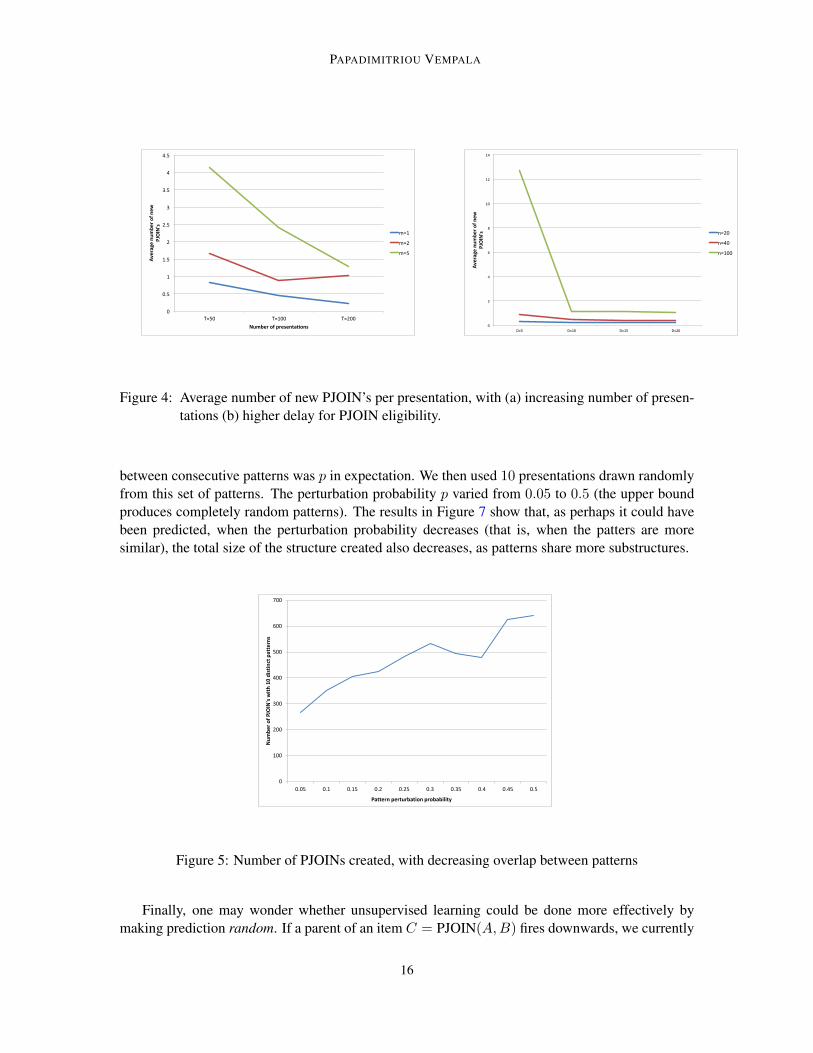
Next, items created in early presentations are relatively stable, with few PJOINS created onlater presentations, as predicted by Theorem 2. Figure 4 shows the average number of new PJOIN’screated in each presentation, as the number of presentations increases, and as the delay for PJOINeligibility (for items that have fired) is increased. For these experiments we kept n at 40 and p =q = 0.1.

Another experiment explores the sharing of common substructures by patterns. We generatedthe patterns by starting with one random pattern with n = 100, and obtain 9 more patterns byperturbing each coordinate of it randomly with probability p. In other words, the Hamming distance

15


0

0.5

1

1.5

2

2.5

3

3.5

4

4.5

T=50 T=100 T=200

Average nu

mbe

r of n

ew

PJOIN's

Number of presenta8ons

m=1

m=2

m=5

0

2

4

6

8

10

12

14

D=5 D=10 D=15 D=20

Average nu

mbe

r of n

ew

PJOIN's n=20

n=40

n=100

Figure 4: Average number of new PJOIN’s per presentation, with (a) increasing number of presen-tations (b) higher delay for PJOIN eligibility.

between consecutive patterns was p in expectation. We then used 10 presentations drawn randomlyfrom this set of patterns. The perturbation probability p varied from 0.05 to 0.5 (the upper boundproduces completely random patterns). The results in Figure 7 show that, as perhaps it could havebeen predicted, when the perturbation probability decreases (that is, when the patters are moresimilar), the total size of the structure created also decreases, as patterns share more substructures.

0

100

200

300

400

500

600

700

0.05 0.1 0.15 0.2 0.25 0.3 0.35 0.4 0.45 0.5

Num

ber o

f PJO

IN's

with

10

dist

inct

pat

tern

s

Pattern perturbation probability

Figure 5: Number of PJOINs created, with decreasing overlap between patterns

Finally, one may wonder whether unsupervised learning could be done more effectively bymaking prediction random. If a parent of an item C = PJOIN(A,B) fires downwards, we currently

16


hb!

0

0.5

1

1.5

2

2.5

Ratio

of m

odel

pre

dict

ion

to o

bser

ved

valu

e

Data from Song et al. 2005

Figure 6: Comparison of the random model with reciprocity data. The first bar in each pair is withp = q = 0.05, the second withp = 0.05, q = 0.047.

require CP to fire downwards to both A and B. One interesting variant would only fire downwardsto one of A and B, chosen at random. This new version of PJOIN would generate considerably lessdownward traffic, and detect new patterns at a slower rate than the current one.

Appendix F: Figure 6

Appendix P: Proofs

First, we give the proof that PJOIN operates as claimed.Proof (of Theorem 1.) We must argue two things: First, that the algorithm Create PJOIN(A,B)above is vicinal, that is, it can be implemented within the model described in Section 2 throughappropriate state transformation functions δ and λ. And second, that the resulting item responds tofirings of other items as specified by the diagram.

For the creation part, and since we assume that JOIN and LINK are implemented correctly, allwe need to show is that the conditions that must fold after the second and after the fourth step ofthe algorithm Create PJOIN(A,B) can be implemented vicinally. The former is the identificationof a random subset CP of C, which is straightforward as discussed. The latter consists of (a) thePARENT memory state of the synapses from CP to AP and BP , and the doubling of the strengths ofthese same synapses. Both (a) and (b) can be accomplished by the function λ of the neuroids rightafter the creation of LINK(CP .AP ) and LINK(CP .BP ).

To argue that the resulting PJOIN(A,B) operates as specified in the diagram, it sufficed to checkeach transition It is easy to see that the transition graph is complete). For example, for the transitionsout of the OPERATIONAL state: The “A andB fire” self-loop follows from the fact that, in this case,

17


PJOIN operates exactly as JOIN. The “P” self-loop is also immediate, since, for each parentD of theitem, the synapses coming fromDP will cause the item to fire. And so on for the other transitions.

For the proof Theorem 2 on learning, we start with a bound on the maximum level of PJOINitems for a single pattern.

Lemma 3 Under the conditions of the theorem, with high probability, the maximum level of an itemis O(log n).

Proof Suppose n sensory items are PJOIN-eligible, so that n−1 PJOINs happen. Order the PJOINs1, 2, . . . , n − 1. Fix a sensory item s and let Xj be the 0-1 random variable that indicates whethers participates in the j’th PJOIN. Then the height of s at the end of the process is X =

∑n−1j=1 Xj .

From this we have,

E(X) ≤n−1∑j=1

1

n− j= Hn−1 < 1 + ln(n− 1).

The claim follows from the Chernoff bound for independent Bernoulli random variables (with pos-sibly different expectations):

Pr(X − E(X) > tE(X)) ≤(

et

(1 + t)(1+t)

)E(X)

≤ (e+ 1)−E(X)

where we used t = e.

Proof ( of Theorem 2.) First we note that any item at any level fires if and only if all its descendantsfire in response to an input pattern. This is clear since an item fires if and only if both its childrenfire or it is an input level item activated by an input symbol. In the former case, this firing criterionrecursively applied, leads to the set of all descendants of the original item, i.e., an item fires iff allits input level descendants fire. Thus, if the descendants of an item C are exactly the set of sensoryitems for a particular pattern x then C fires if and only if x is presented.

Next we claim that with high probability, when a new pattern x is encountered, the algorithmcreates a new highest level cell to represent this pattern, i.e., the first presentation of the pattern xcreates an item I(x) whose descendants include all n sensory items that fire for x. After all possibleprocessing of items according to the operational PJOIN state transition rules (see Fig. 1), if thereis currently no item whose descendants match the pattern x, there must be a set of items S thatare PJOIN-eligible. New items are then created by sampling a pair of items from S performing aPJOIN and adding the resulting item to S. This process finishes with a single item after |S|−1 suchPJOIN’s. The descendants of this item correspond to the pattern x.

Now consider the presentation of a pattern x for which we already have a top-level item I(x).All items whose descendants match the pattern will eventually fire. Thus, the original highest-levelitem for x will eventually fire, as claimed. En route, it is possible that two items that have fired,but none of whose parent items have fired as yet, will try to form a new PJOIN. First we bound thetotal number of rounds. Independent of the PJOIN creation, in each round, each sensor fires withprobability p. Thus, with high probability, all n sensor items fire within (2 lnn)/p rounds. Theadditional number of rounds after all sensors fire is at most the depth of the tree, i.e., at most 4 lnn

18


whp. So the total number of rounds, again with high probability, is at most 4 lnn+(2 lnn)/p. Thusour bound on T is adequate.

Next, on a presentation of x, consider any PJOIN item A with a parent B that is a descendantof I(x). After item A fires, it will become PJOIN-eligible after D steps. But after A fires, its parentB predicts its sibling. The sibling is at level at most `(A), and therefore it will fire within at most2`(A) + 2 steps. Therefore such an item A will not be PJOIN-eligible after D steps since its parentwould have fired.

Now consider the point where all sensor items have been sampled and existing PJOIN itemsthat will fire, including I(x) have fired. There might be items that have fired but whose parents didnot fire, items that are valid for x, but were created during the presentation of a different pattern y.These items can now form new PJOINs. However, after seeing each of the m input patterns at leastonce, no new PJOIN items will be created at level 1. This is because each sensory item, for eachpattern, has at least one PJOIN parent. After another round of seeing allm input patterns, no PJOINitems are created at level 2. If we bound the maximum level of items, then this will bound themaximum number of rounds of seeing all m patterns after which no new PJOIN items are created.

In fact, the maximum level of an item will be O(log n + logm). To see this, we we can eitheruse Lemma 4 or the following more direct argument (with a slightly weaker bound) to concludethat the maximum number of items at level ` is at most mn/2`. Fix a pattern i and suppose the firstpattern and the i’th pattern share an r fraction of the sensor items. Then at level 1, some fraction ofthese rn sensors on which they agree will form PJOINs among themselves. The sensors involved insuch PJOINs will no longer form new PJOINs on presentation of patterns 1 or i, since they alreadyhave PJOIN parents that will fire. The remaining common sensors could form new PJOINs that arevalid for both 1 and i in later presentations of 1 or i. But no matter how many such PJOINs (amongthe common items) are formed on each presentation, the total number that can be valid for both 1and i at level 1 is at most rn/2, since once a sensor participates in one such PJOIN (where the othersibling is also from the common set of r.n sensors), it will no longer do so. For all m patterns, thenumber of PJOINs at level 1 valid for pattern 1 and any other pattern is at most mn/2.

We continue this argument upward. Of the items at level 1 (at most rn/2) that are valid for both1 and i, on a presentation of i, some pairs could form new PJOINs that are valid for both 1 and i,if they do not already have such PJOIN parents with both children valid for both patterns, but nomatter what order this happens, there can be at most rn/4 such PJOINs at level 2. This continues,with the number of PJOIN items halving at each level. Therefore, after O(log n + logm) roundsof seeing all input patterns (in arbitrary order, and any positive number of times in each round), nofurther PJOINs are created and the top-level items are stable for each pattern.

The next lemma gives a sharp bound on the number of PJOIN items valid for two differentpatterns.

Lemma 4 Let ri = 1 − 1nH(x1, xi) be the fraction of overlap between two patterns x1 and xi,

where H is the Hamming distance. The expected number of PJOINs created at level ` that are valid

19


(i.e., will fire) for patterns x1 and xi is (n/2)(r4i + r2i (1− r2i )(1 + 1(1+r)2

)) for ` = 1 and

n

2`·

r2`+1

i + r2`

i (1− r2`i ) ·

1 +

1 +

(1+(...)2

1+r2`−1

i

)2

1 + r2`

i

2 <

n

2`.

for higher `. Moreover, whp, the number of such PJOINs will be within a factor of 4 of this bound.

Proof The proof of the expectation is by induction on `. Consider two patterns x1 and x2 and letr be the fraction of sensors where they agree. Then on the first presentation of x1, the number ofPJOIN items created at level ` is n/2`, and the expected fraction of them that are also valid for x2will be r2

`(since all constituent sensor items must be drawn from the common r fraction). Now,

on a presentation of x2, there might be more PJOINs created that are valid for x1. At level 1, suchPJOINs will come from sensors that are valid for both, but do not yet participate in PJOINs that arevalid for both. The expected fraction of such sensors is r − r2 = r(1 − r). For each such sensor,to be part of a new PJOIN valid for x1, the other sensor must also be picked from this set. The totalfraction of sensors participating in the creation of PJOINS will be 1 − r2, since an r2 fraction ofsensors already have PJOINs that will fire. Thus, the expected number of new PJOINs created atlevel 1 will be

n

2· r(1− r) · r(1− r)

1− r2=n

2· r2(1− r2) · 1

(1 + r)2

and thus the total number in expectation at level 1 is as claimed.To compute the expected number of PJOINs created at the next level, we note that the first

presentation of x1 creates r4 ·(n/4) PJOINs that are valid for both x1 and x2. When x2 is presented,the PJOIN items at level one that become PJOIN-eligible are r2(1− r2)(1 + (1/(r + 1)2) · (n/2),with the first term coming from PJOINs that were created on the presentation of x1 and the secondfrom new PJOINs created during the first presentation of x2. Thus the number of PJOINs created atlevel 2 in expectation will be n/4 times(

r2(1− r2)(1 + 1

(1+r)2

))21− r4

= r4(1− r4)

(1 + 1

(1+r)2

1 + r2

)2

.

Thus, the total number of PJOIN-eligible items at level 2 in expectation is

n

4·

r4 − r8 + r4(1− r4)

(1 + 1

(1+r)2

1 + r2

)2 =

n

4

(r4(1− r4)f(2)

).

Continuing, the expected number of PJOIN eligible items at level 3 is (n/8) times

r8(1− r8) +(r4(1− r4)f(2)

)21− r8

= r8(1− r8)

(1 +

(f(2)

1 + r4

)2)

= r8(1− r8)f(3).

At the `’th level, the expected number of PJOIN-eligible items is thus (n/2`) times

r2`(1− r2`)f(`) where f(`) = 1 +

(f(`− 1)

1 + r2`−1

)2

.

20


Adding the number of PJOINs at level ` created by the first presentation of x1 that are valid for bothx1 and x2 and participated in PJOINs valid for both at the next level on the first presentation of x1,which is (n/2`)r2

`+1, gives the claimed bound.

We proceed to show the inequality, namely that the above quantity, r2`(1−r2`)f(`), is bounded

by 1− r2`+1for any r ∈ [0, 1], by induction on `. In fact, our induction hypothesis is the following:

f(`) ≤ 1 +1

r2`

It holds for ` = 2. Assuming the induction hypothesis for `− 1,

f(`) = 1 +

(f(`− 1)

1 + r2`−1

)2

≤ 1 +

(1 + 1

r2`−1

1 + r2`−1

)2

= 1 +1

r2`

Thus, r2`(1− r2`)f(`) ≤ (1− r2`)(1 + r2

`) ≤ 1− r2`+1

.The high probability bound follows from the independence of the PJOINs at each level.

21

cortical learning via prediction

Documents