Simulation

COS 323

Last Time

•  Stability of ODEs

•  Stability of PDEs

•  Review of methods for solving large, sparse systems

•  Multi-grid methods

Reminders

•  Homework 4 due Tuesday

•  Homework 5, final project proposal due Friday December 16

Today

•  Simulation examples

•  Discrete event simulation – Time-driven and event-driven approaches, with

examples – Cellular automata, microsimulation, agent-based

simulation

•  Population genetics overview

Why simulation?

•  Make predictions or make decisions regarding complex phenomena or poorly-understood phenomena

•  Test theories about how real systems work

•  Explore consequences of changes to a system

•  Train people to make better decisions or take correct actions

•  …

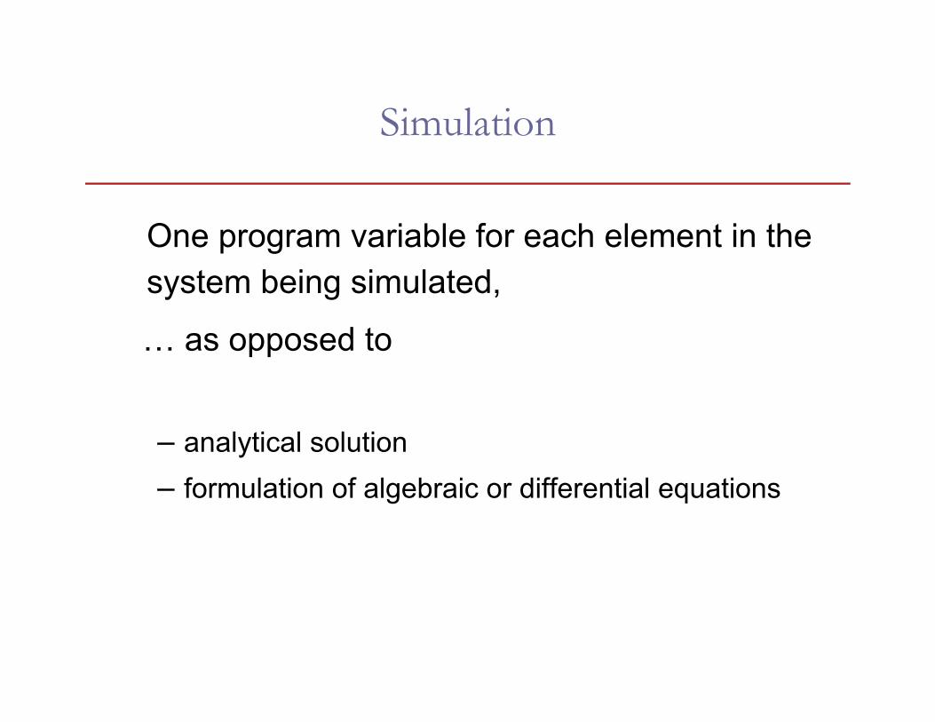
Simulation

One program variable for each element in the system being simulated,

… as opposed to

–  analytical solution –  formulation of algebraic or differential equations

Approaches to Simulation

•  Differential equation solvers can be thought of as conducting a simulation of a physical system – Advance through time –  “Continuous” equations model change in state

•  Some simulations are more “discrete”: – Decisions, actions, events happen at discrete

points in time

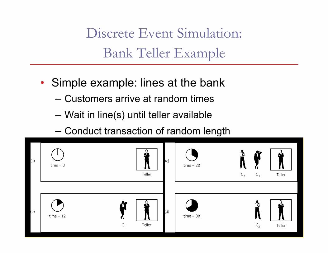
Discrete Event Simulation: Bank Teller Example

•  Simple example: lines at the bank – Customers arrive at random times – Wait in line(s) until teller available – Conduct transaction of random length

Bank Teller

•  Simple example: lines at the bank – Customers arrive at random times – Wait in line(s) until teller available – Conduct transaction of random length

•  Simulate arbitrary phenomena (e.g. spike in customer rate during lunch)

•  Goal: mean and variance of waiting times – As a function of customer rate, # tellers, # queues

Bank Teller

•  Time-driven simulation: – A master clock increments time in fixed-length

steps – At each step, compute probability of customer(s)

arriving, determine whether any transactions finishing

•  e.g., probability of 2% that a new customer arrives at each time step

– More accurate simulation with shorter time steps, but then have more steps when nothing happens

Bank Teller

•  Event-driven simulation: –  Events change system state:

•  New customer arrives

•  Teller finishes processing a customer

–  Compute times of events and put in a “future event list”: •  When will new customers arrive? •  When new customer reaches teller, compute time that

customer will finish.

–  Repeatedly process one event, then fast-forward until scheduled time of next event

–  Good accuracy and efficiency: automatically use time steps appropriate for how much is happening

Time-driven Example: Epidemics

The SIR Model

•  W. O. Kermack and A. G. McKendrick, 1929

•  susceptible: susceptible, not yet infected

•  infected: infected and capable of spreading

•  recovered / removed: recovered and immune

Time-Driven Simulation: Epidemics

•  [Dur95] R. Durrett, "Spatial Epidemic Models," in Epidemic Models: Their Structure and Relation to Data, D. Mollison (ed.), Cambridge University Press, Cambridge, U.K., 1995.

•  Discrete-time, discrete-space, discrete-state

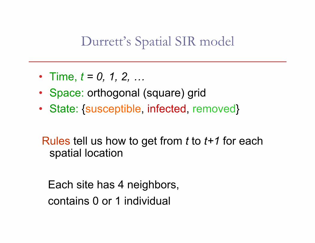
Durrett’s Spatial SIR model

•  Time, t = 0, 1, 2, … •  Space: orthogonal (square) grid •  State: {susceptible, infected, removed}

Rules tell us how to get from t to t+1 for each spatial location

Each site has 4 neighbors, contains 0 or 1 individual

Durrett’s Rules for Spatial SIR model

•  Susceptible individuals become infected at rate proportional to the number of infected neighbors

•  Infected individuals become healthy (removed) at a fixed rate δ

•  Removed individuals become susceptible at a fixed rate α

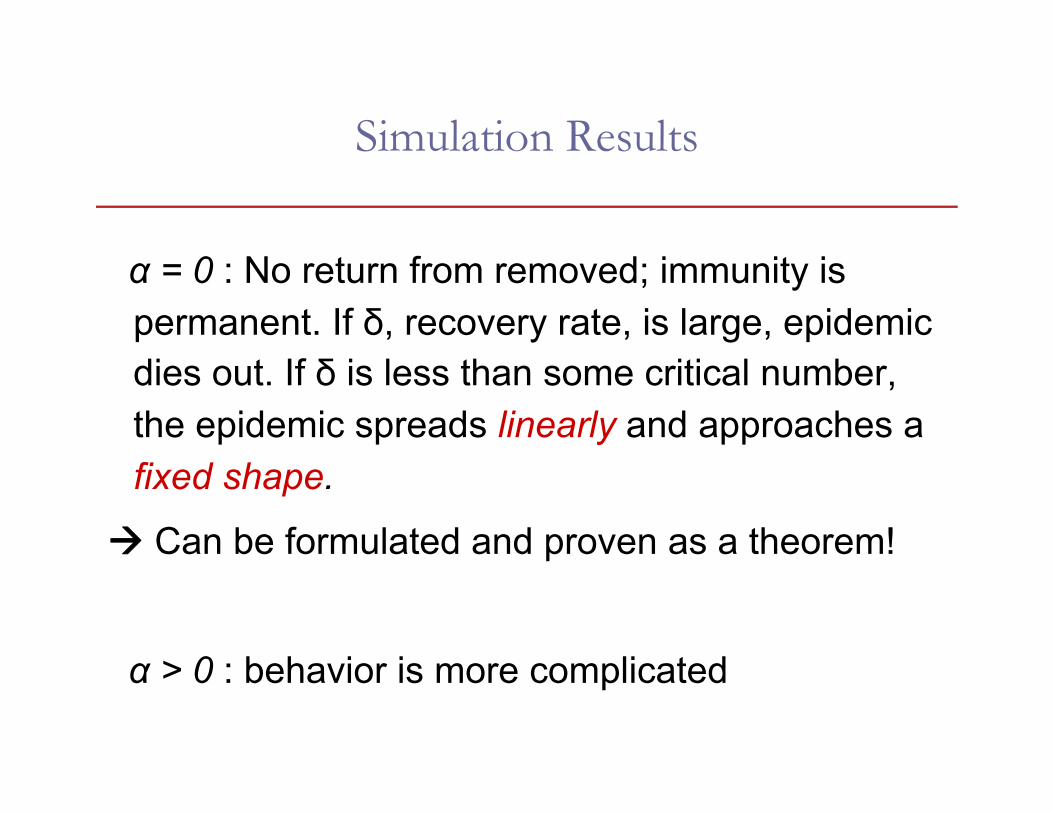
Simulation Results

α = 0 : No return from removed; immunity is permanent. If δ, recovery rate, is large, epidemic dies out. If δ is less than some critical number, the epidemic spreads linearly and approaches a fixed shape.

Can be formulated and proven as a theorem!

α > 0 : behavior is more complicated

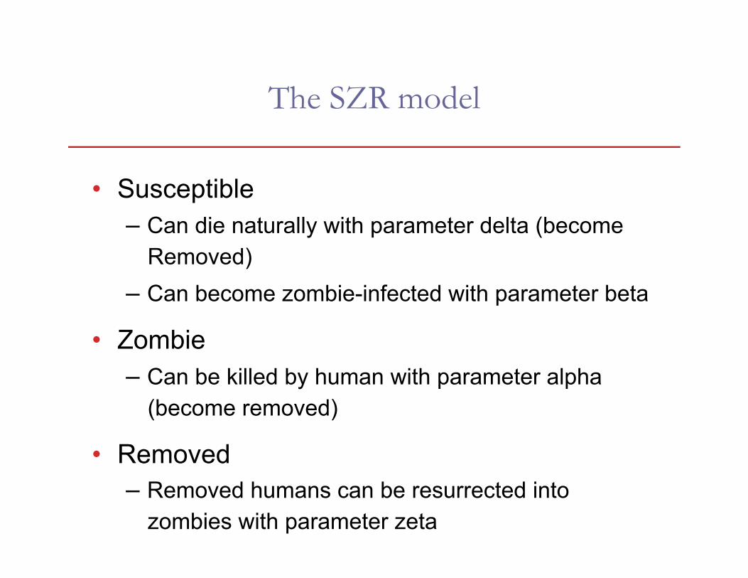
The SZR model

•  Susceptible – Can die naturally with parameter delta (become

Removed) – Can become zombie-infected with parameter beta

•  Zombie – Can be killed by human with parameter alpha

(become removed)

•  Removed – Removed humans can be resurrected into

zombies with parameter zeta

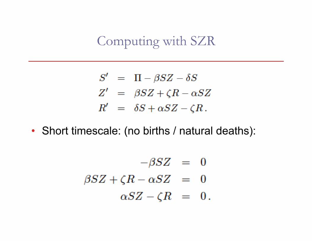
Computing with SZR

•  Short timescale: (no births / natural deaths):

Using Euler’s Method

Model with Latent Infection

Alternative Zombie Sim

•  http://kevan.org/proce55ing/zombies/

Event-Driven Examples

Example: Load Balancing Across Hosts

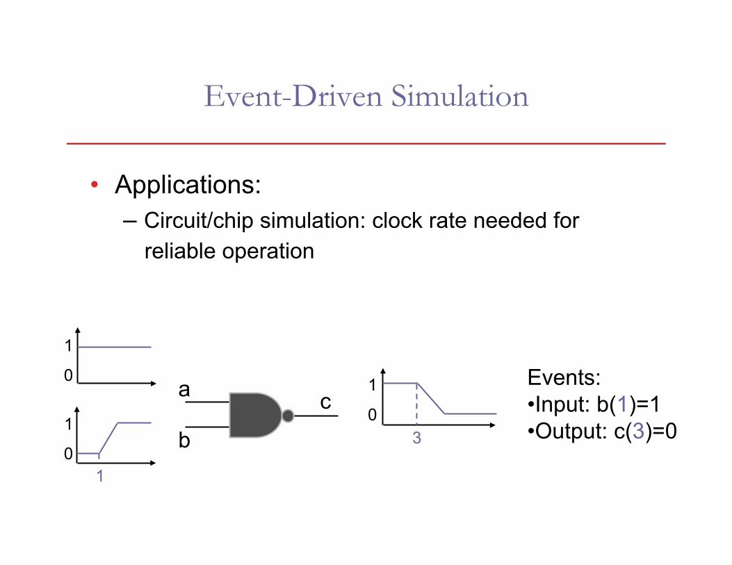
Event-Driven Simulation

•  Applications: – Circuit/chip simulation: clock rate needed for

reliable operation

1 0

1

0

1

0

1 a

b

c Events: • Input: b(1)=1 • Output: c(3)=0 3

Event-Driven Simulation

•  Applications: – Circuit/chip simulation: clock rate needed for

reliable operation

a

b

c

d

e

Ingredients of Event-Driven Simulations

•  Event queue – Holds (time, event) tuples – Priority queue data structure: supports

fast query of event with lowest time – Possible implementation: linked list

O(n) insertion, O(1) query, O(1) deletion – Possible implementation: heap, binary tree

O(log n) insertion, O(1) query, O(log n) deletion

Ingredients of Event-Driven Simulations

•  Event loop – Pull lowest-time event off event queue – Process event

•  Decode what type of event •  Run appropriate code •  (Compile statistics) •  Insert any new events onto queue

– Repeat.

Ingredients of Event-Driven Simulations

•  How are new events scheduled? – Some are a direct result of current event.

Example: teller takes new customer – Some are background events.

Example: new customer arrives – Some are generated via real-time user input

Stochastic Simulation

•  Events have different likelihoods of occurrence – New customer arrives – Person contracts disease

•  Properties of simulation components may vary – Bank customers may have more or less difficult

problems – Drivers may be more or less polite –  Individuals may be more or less susceptible to

disease

Sources of “Randomness”

•  “Digital Chaos”: Deterministic, complicated. Examples: pseudorandom RNGs in code, digital slot machines.

•  “Analog Chaos”: Unknown initial conditions. Examples: roulette wheel, dice, card shuffle, analog slot machines.

•  “Truly random”: Quantum mechanics. Examples: some computer hardware-based RNGs

“Anyone who considers arithmetical methods of producing random digits is, of course, in a state of sin.”

--- John von Neumann (1951)

Using RNGs

How would you…

•  Choose an integer i between 1 and N randomly

•  Choose from a discrete probability distribution; example: p(heads) = 0.4, p(tails) = 0.6

•  Pick a random point in 2-D: square, circle

•  Shuffle a deck of cards

Bank Simulation: Scheduling Arrival Events

•  Given time of last customer arrival, how to generate time of next arrival?

•  Assume arrival rate is uniform over time: k customers per hour

•  Then in any interval of length Δt, expected number of arrivals is k Δt

Scheduling Arrival Events

•  Probability distribution for next arrival? – Equal to probability that there are no arrivals

before time t – Subdivide into intervals of length Δt

p(no arrivals before t) = p(no arrival between 0 and Δt) * p(no arrival between Δt and 2Δt) * …

Scheduling Arrival Events

•  p(no arrival in interval) = 1 – k Δt

•  So, p(no arrivals before t) =

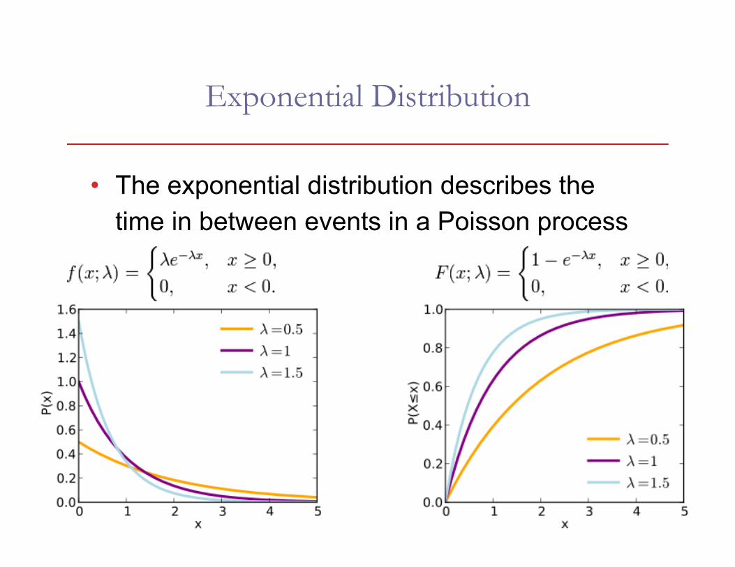
Exponential Distribution

•  The exponential distribution describes the time in between events in a Poisson process

Sampling from a non-uniform distribution

•  “Inversion method” –  Integrate f(x): Cumulative Distribution Function –  Invert CDF, apply to uniform random variable

Sampling from the Exponential Distribution

•  time to next arrival event can be found from uniform random variable ξ ∈ [0..1] via

Ingredients of Event-Driven Simulations

•  How are events handled? – Need to run different piece of code depending on

type of event – Code needs access to data: which teller?

which customer? – Original motivation for Object-Oriented

Programming languages: encapsulate data and code having a particular interface

– First OO language: Simula 67

Summary

•  Insert events onto queue

•  Repeatedly pull them off head of queue – Decode – Process – Add new events

CAs, Microsimulation and Agent-based Simulation

(Micro-level behaviors leading to emergent macro-level phenomena)

Cellular Automaton

•  Discrete-time, discrete-space model

•  Cells in grid have finite number of states

•  Each cell’s new state is a function of its previous state and the previous states of its neighbors – Typically instantaneous updates, same rules for all

cells

Microsimulation

•  Model components of system as independent entities with differing characteristics –  e.g., different susceptibility to disease

•  Behavior is governed by particular rules

•  Useful in traffic, health, econometrics (e.g., taxation)

•  Demo: –  http://www.traffic-simulation.de/

Agent-Based Modeling

•  Accommodates interdependencies, adaptive behaviors

•  E.g., “The evolution of cooperation”

The Prisoner’s Dilemma

•  Globally optimal: Neither confesses

•  Game-theoretically optimal strategy: Always confess

The Evolution of Cooperation

•  Robert Axelrod: A tournament for simulations to play with each other in repeated rounds

•  Winning strategy: TFT

•  All top strategies are “nice”

•  Necessary conditions for success: – Be nice – Be provocable – Don’t be envious – Don’t be too clever

A better strategy

•  Jennings et al. in 2004 tournament: – Submit multiple prisoners and collude

Simulating Population Genetics

Simulating population genetics (assignment 5)

•  review of basic genetics: genes, alleles

•  If there are two possible alleles at one site, say A and a, there are in a diploid organism three possible genotypes: AA, aa, Aa, the first two homozygotes, the last heterozygote

•  Question: How are these distributed in a population as functions of time?

Why study this?

•  Understanding history of evolution, human migration, human diversity

•  Understanding relationship between species

•  Understanding propagation of genetic diseases

•  Agriculture

Approaches, pros and cons

•  Field experiment + realistic - hard work for one particular situation •  Mathematical model + can yields lots of insight, intuition - usually uses very simplified models - not always tractable •  Simulation + very flexible + works when math doesn’t - not easy to make predictions

19th Century: Darwin et al. didn’t know about genes, etc., and used the idea of blended inheritance

 But this requires an unreasonably large mutation rate to explain variation, evolution

Enter Mendel… (rediscovered in 20th century)

Gregor Mendel (1822 - 1884)

http://bio.winona.edu/berg/241f00/Lec-note/Mendel.htm

Steven Berg, Winona State

Simplest Model

•  Hardy-Weinberg equilibrium –  If probability of allele A is p, of a is q=1-p

p(AA) = p2, p(Aa) = 2pq, p(aa) = q2

•  Not always observed – Wahlund effect: fewer heterozygotes if multiple

isolated subpopulations – Differences in viability, mating preference

•  Assignment 5: limitations of theoretical model – Finite population, others