cosmosm electromagnetics module (estar) - …fem/docs/cosmosm/estar.pdf · estar is a finite...
TRANSCRIPT

Contents
1 Introduction . . . . . . . . . . . . . . . . . . . . . . . . . . . . . . . . . . 1-1
Introduction . . . . . . . . . . . . . . . . . . . . . . . . . . . . . . . . . . . . . . . . . . . . . . . . . .1-1Theory . . . . . . . . . . . . . . . . . . . . . . . . . . . . . . . . . . . . . . . . . . . . . . . . . . . . . .1-2
Two Dimensional Analysis . . . . . . . . . . . . . . . . . . . . . . . . . . . . . . . . . . . .1-2Three Dimensional Analysis . . . . . . . . . . . . . . . . . . . . . . . . . . . . . . . . . . .1-4Three Dimensional Current Sources . . . . . . . . . . . . . . . . . . . . . . . . . . . . .1-5Electrostatic Analysis . . . . . . . . . . . . . . . . . . . . . . . . . . . . . . . . . . . . . . . .1-5
Finite Element Formulation . . . . . . . . . . . . . . . . . . . . . . . . . . . . . . . . . . . . . .1-6
2 Analysis Options . . . . . . . . . . . . . . . . . . . . . . . . . . . . . . 2-1
Introduction . . . . . . . . . . . . . . . . . . . . . . . . . . . . . . . . . . . . . . . . . . . . . . . . . .2-1Analysis Options . . . . . . . . . . . . . . . . . . . . . . . . . . . . . . . . . . . . . . . . . . . . . .2-1Solver Type . . . . . . . . . . . . . . . . . . . . . . . . . . . . . . . . . . . . . . . . . . . . . . . . . .2-2Material Properties . . . . . . . . . . . . . . . . . . . . . . . . . . . . . . . . . . . . . . . . . . . .2-2Unit System . . . . . . . . . . . . . . . . . . . . . . . . . . . . . . . . . . . . . . . . . . . . . . . . . .2-2Nonlinearities . . . . . . . . . . . . . . . . . . . . . . . . . . . . . . . . . . . . . . . . . . . . . . . .2-2 Postprocessing Results . . . . . . . . . . . . . . . . . . . . . . . . . . . . . . . . . . . . . . . . .2-3
Two Dimensional Analysis and Axisymmetric Analysis . . . . . . . . . . . . .2-4Three Dimensional Analysis . . . . . . . . . . . . . . . . . . . . . . . . . . . . . . . . . . .2-4
3 Description of Elements . . . . . . . . . . . . . . . . . . . . . . . . . 3-1
Introduction . . . . . . . . . . . . . . . . . . . . . . . . . . . . . . . . . . . . . . . . . . . . . . . . . .3-1
COSMOSM Advanced Modules 1

Contents
2
4 Brief Description of Commands . . . . . . . . . . . . . . . . . . . 4-1
Introduction . . . . . . . . . . . . . . . . . . . . . . . . . . . . . . . . . . . . . . . . . . . . . . . . . .4-1MPROP (Propsets > Material Property) Command . . . . . . . . . . . . . . . . .4-1
Commands Likely to be Used for a Given Analysis . . . . . . . . . . . . . . . . . . .4-2LoadsBC > FLUID FLOW > BOUND ELEMENT . . . . . . . . . . . . . . . . .4-2LoadsBC > E_MAGNETIC POTENTIAL . . . . . . . . . . . . . . . . . . . . . . . .4-3LoadsBC > E_MAGNETIC > MAGNETIC POTENTIAL . . . . . . . . . . .4-4LoadsBC > E-MAGNETIC > NODAL CURRENT . . . . . . . . . . . . . . . . .4-5LoadsBC > E-MAGNETIC > ELEMENT CURRENT . . . . . . . . . . . . . . .4-6LoadsBC > FUNCTION CURVE . . . . . . . . . . . . . . . . . . . . . . . . . . . . . . .4-7
Analysis Menu . . . . . . . . . . . . . . . . . . . . . . . . . . . . . . . . . . . . . . . . . . . . . . .4-7Analysis > ELECTRO MAGNETIC . . . . . . . . . . . . . . . . . . . . . . . . . . . . .4-7
Results Menu . . . . . . . . . . . . . . . . . . . . . . . . . . . . . . . . . . . . . . . . . . . . . . . . .4-8
5 Detailed Description of Examples . . . . . . . . . . . . . . . . . 5-1
Introduction . . . . . . . . . . . . . . . . . . . . . . . . . . . . . . . . . . . . . . . . . . . . . . . . . .5-13D Permanent Magnet With an Air Gap Example . . . . . . . . . . . . . . . . . . . .5-1Magnetic Field for Two Parallel Conductors Example . . . . . . . . . . . . . . . .5-17
6 Verification Problems . . . . . . . . . . . . . . . . . . . . . . . . . . 6-1
Introduction . . . . . . . . . . . . . . . . . . . . . . . . . . . . . . . . . . . . . . . . . . . . . . . . . .6-1
COSMOS/M Advanced Modules

1 Introduction
Introduction
ESTAR is a finite element based program for solving electromagnetic problems. The main capabilities of this program are:
• Magnetostatic analysis for two dimensional and axisymmetric problems with current sources and permanent magnets.
• Magnetostatic analysis of general three dimensional models with permanent magnets and current sources.
• Electrostatic and current flow analyses of two and three dimensional models.
• Transient electromagnetic analysis for two dimensional and axisymmetric problems.
• AC (time harmonic) eddy current analysis for two dimensional and axisymmetric problems.
• Ability to use the result outputs for electro-thermal and magneto-structural coupling analyses.
• Capacitance matrix calculation for multi-conductor transmission lines.
• Nonlinear analysis: B-H material curves and/or permanent magnet demagnetization curves.
• Result outputs: Magnetic flux density, field intensity, forces, torque, inductance, capacitance matrix, input energy, stored energy and coenergy, voltage, electric field, induced eddy currents and power loss.
COSMOSM Advanced Modules 1-1

Chapter 1 Introduction
1-2
Theory
The theory used in ESTAR program is based on the application of the potential function theory to Maxwell's equations. Magnetic vector and scalar potentials are used for two and three dimensional analysis, respectively. The resulting equations used in finite element analysis are outlined here.
The Maxwell's equations are the following:
1-1
1-2
1-3
1-4
where H and E are the magnetic and electric fields, B and D are the magnetic and electric flux densities, J is the conduction current density, and ρ is the electric charge density. The constitutive equations are:
B = µ (B) (H + Hc) 1-5
J = σ E 1-6
D = e E 1-7
where σ is electric conductivity, m is magnetic permeability, ε is electric permittivity, and Hc is the coercivity of permanent magnets.
Two Dimensional Analysis
Flux density B may be expressed as a function of a vector potential A such that
1-8
where A satisfies the following uniqueness condition
1-9
COSMOSM Advanced Modules

Part 2 ESTAR / Low Frequency Electromagnetic Analysis
Using equations (1-8) and (1-5) in equations (1-1) and (1-2) and neglecting the term , the following equations would yield
1-10
1-11
where ν is reluctivity (ν = 1/ µ). The equation (1-11) implies
1-12
where φ is the reduced electric scalar potential. Combining this equation with the constitutive equation (1-6) it results
1-13
Total current density in equation (1-10) may consist of the source current Js and eddy current Je, hence equation (1-10) may take the following for m
1-14
For the two dimensional models in the x-y plane, the only non zero components of A and ∇ φ are the z components which are functions of x and y only and do not vary in the z direction. Therefore the above equation takes the following scalar form
1-15
For the axisymmetric case, taking z in the azimuthal direction the only non zero component of A is the azimuthal component. For this case equation (1-14) reduces to the following scalar form
1-16
For the axisymmetric case, x and y correspond to radial and axial components of cylindrical coordinates. Two dimensional and axisymmetric analysis in ESTAR are based on equations (1-15) and (1-16), respectively.
For time harmonic AC analysis the current source density is assumed to be of the form
Js = J0 eiwt 1-17
COSMOSM Advanced Modules 1-3
Chapter 1 Introduction
1-4
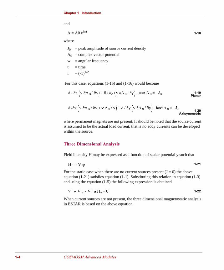
and
A = A0 eiwt 1-18
where
J0 = peak amplitude of source current density
A0 = complex vector potential
w = angular frequency
t = time
i = (-1)1/2
For this case, equations (1-15) and (1-16) would become
1-19 Planar
1-20 Axisymmetric
where permanent magnets are not present. It should be noted that the source current is assumed to be the actual load current, that is no eddy currents can be developed within the source.
Three Dimensional Analysis
Field intensity H may be expressed as a function of scalar potential y such that
1-21
For the static case when there are no current sources present (J = 0) the above equation (1-21) satisfies equation (1-1). Substituting this relation in equation (1-3) and using the equation (1-5) the following expression is obtained
1-22
When current sources are not present, the three dimensional magnetostatic analysis in ESTAR is based on the above equation.
COSMOSM Advanced Modules
Part 2 ESTAR / Low Frequency Electromagnetic Analysis
Three Dimensional Current Sources
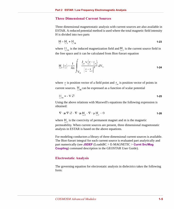
Three dimensional magnetostatic analysis with current sources are also available in ESTAR. A reduced potential method is used where the total magnetic field intensity H is divided into two parts
1-23
where is the induced magnetization field and is the current source field in
the free space and it can be calculated from Biot-Savart equation
1-24
where is position vector of a field point and is position vector of points in
current sources. can be expressed as a function of scalar potential
1-25
Using the above relations with Maxwell's equations the following expression is obtained:
1-26
where is the coercivity of permanent magnet and m is the magnetic
permeability. When current sources are present, three dimensional magnetostatic analysis in ESTAR is based on the above equations.
For modeling conductors a library of three dimensional current sources is available. The Biot-Savart integral for each current source is evaluated part analytically and part numerically (see JSDEF (LoadsBC > E-MAGNETIC > Curnt Src/Mag Coupling) command description in the GEOSTAR User Guide).
Electrostatic Analysis
The governing equation for electrostatic analysis in dielectrics takes the following form:
COSMOSM Advanced Modules 1-5

Chapter 1 Introduction
1-6
1-27
where ε is the dielectric constant, r is the charge density.
Boundary Conditions
Available boundary conditions are of the following forms:
1. The value of the electric or magnetic potential is prescribed (Dirichlet boundary condition). It should be noted that the constant potential value at a boundary for two dimensional magnetic analysis produces flux lines that are parallel to the boundary and for three dimensional magnetic analysis produces flux lines that are perpendicular to the boundary.
2. The value of the normal derivative of the magnetic potential is prescribed (Neumann boundary condition). It should be noted that homogeneous Neumann boundary conditions (when the prescribed values are zero) are automatically satisfied in the finite element formulation.
3. Multiple constraints, which can be used when the potential variables have the same values at corresponding points, this option can be used to specify periodic type boundary conditions (see verification problem EM16).
4. The boundary conditions at infinity can be imposed for magnetostatic and electrostatic problems with infinite domains by placing infinite elements at the boundary of the model. These elements should be placed on convex type boundaries and they should be away from the coordinate axis of the model (see verification problem EM17 and EM18).
Finite Element Formulation
The finite element method used in ESTAR is based on stationarity of suitable energy functionals for equations (1-15), (1-16), (1-23), (1-26) and (1-27). For nonlinear problems, a Newton-Raphson method is used which can be expressed in the following matrix form:
1-28
COSMOSM Advanced Modules

Part 2 ESTAR / Low Frequency Electromagnetic Analysis
where:
= Linear stiffness matrix at time t + D t
= Nonlinear stiffness matrix at time t + D t
= Loading vector at time t + D t
= Magnetic potential increment vector at iteration (i)
= Magnetic potential vector at iteration (i-1)
References
1. J. D. Kraus, "Electromagnetics," McGraw-Hill, 3rd Ed. 1984.
2. C. W. Steele, "Numerical Computation of Electric and Magnetic Fields," Van Nostrand Reinhold Co., 1987.
3. P. P. Silvester and R. L. Ferrari, "Finite Elements for Electrical Engineers," Cambridge University Press, UK., 1983.
4. P. Silvester and M. V. K. Chari, "Finite Element Solution of Saturable Magnetic Field Problems," IEEE Trans. Power App. & Syst., V89, 1970, pp. 1642-1651.
5. P. Silvester, H. S. Cabayan and B. T. Browne, "Efficient Techniques for Finite Element Analysis of Electric Machines," IEEE Trans. Power App. & Syst., V92, 1973, pp. 1274-1281.
6. J. Simkin and C. W. Trowbridge, "Three-dimensional Nonlinear Electromagnetic Field Computations, Using Scalar Potentials," IEEE PROC., V127, pt. B, No. 6, 1980, pp. 368-374.
7. S. C. Tandon, A. F. Armor and M. V. K. Chari, "Nonlinear Transient Finite Element Field Computation for Electrical Machines and Devices," IEEE Trans., Power App. & Syst,. V102, No 5, 1983, pp. 1089-1096.
COSMOSM Advanced Modules 1-7

Chapter 1 Introduction
1-8
8. J. L. Coulomb, "A Methodology for the Determination of Global Electromechanical Quantities from Finite Element Analysis and Its Application to the Evaluation of Magnetic Forces, Torques and Stiffness," IEEE Trans. on Magnetics, V19, 1983, pp. 2514-2519.
9. J. L. Coulomb and G. Meunier, "Finite Element Implementation of Virtual Work Principle for Magnetic or Electric Force and Torque Computation," IEEE Trans. on Magnetics, V20, 1984, pp. 1894-1896.
10. J. L. Coulomb, G. Meunier, J. C. Sabonnadiere, "Energy Methods for the Evaluation of Global Quantities and Integral Parameters in a Finite Element Analysis of Electromagnetic Devices," IEEE Trans. on Magnetics, V21, 1985, pp. 1817-1822.
11. C. W. Trowbridge, "Electromagnetic Computing: The Way Ahead ?," IEEE Trans. on Magnetics, V24, No.1, 1988, pp. 13-18.
COSMOSM Advanced Modules

2 Analysis Options
Introduction
This chapter covers all types of analysis, material properties, and postprocessing results in ESTAR.
Analysis Options
There are six analysis options available in ESTAR. The options are chosen through A_MAGNETIC (Analysis > ELECTRO MAGNETIC > Analysis Options) commands and they are as follows:
S for linear and nonlinear magnetostatic analysis
T for transient eddy current analysis
E for electrostatic analysis in dielectrics
C for current flow analysis in conductors
F for time harmonic AC analysis
CAP for capacitance matrix calculations
COSMOSM Advanced Modules 2-1

Chapter 2 Analysis Options
2-2
Solver Type
There are two types of equation solvers available for electrostatic and magnetostatic analyses: the direct Gaussian Solver and the iterative Preconditioned Conjugate Gradient (PCG) Solver. For large size problems, the PCG option can drastically reduce the solution time. The minimum problem size for using the PCG option is 400 and 1000 nodes for 2D and 3D problems, respectively. This option is chosen through the A_MAGNETIC (Analysis > ELECTRO MAGNETIC > Analysis Options) command.
Material Properties
Material properties consist of permeability, electric conductivity in x, y and z directions, permittivity, and remanent magnetization or coercivity of permanent magnets.
Unit System
There are two unit systems available, namely CGS and MKS. Once a unit system is chosen all the properties including geometry and loading has to be provided consistent with the chosen unit.
Nonlinearities
Nonlinear material models consist of B-H curves and permanent magnet demagnetization curves. The B-H material curve is provided by input up to 100 isolated points on the curve, and each curve has to have a minimum of 4 points.
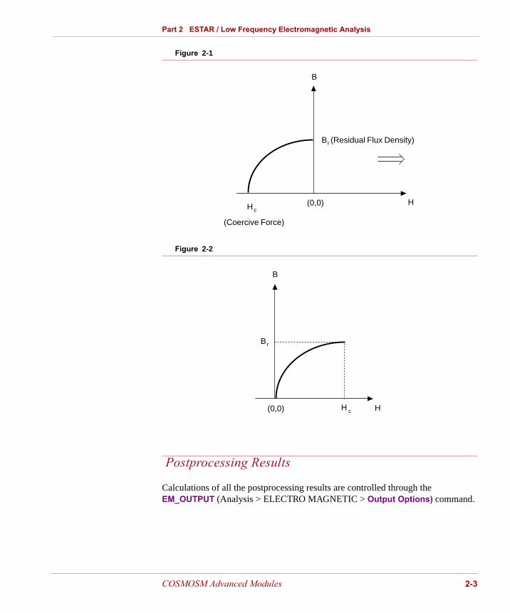
Since the permanent magnet demagnetization curve is in the second quadrant of the B-H curve (see Figure 2-1) it is input as if it were shifted to the first quadrant as shown in Figure 2-2. Hence the first point (Hc,0) is input as (0,0) and the last point (0,Br) is input as (Hc,Br). In addition, the user has to input the values of the three components of the coercivity (coercive force) vector.
COSMOSM Advanced Modules
Part 2 ESTAR / Low Frequency Electromagnetic Analysis
Figure 2-1
Figure 2-2
Postprocessing Results
Calculations of all the postprocessing results are controlled through the EM_OUTPUT (Analysis > ELECTRO MAGNETIC > Output Options) command.
B
HH (0,0)
B (Residual Flux Density)
(Coercive Force)
c
r
B
H(0,0) H c
B r
COSMOSM Advanced Modules 2-3

Chapter 2 Analysis Options
2-4
Two Dimensional Analysis and Axisymmetric Analysis
For two dimensional and axisymmetric analysis the following quantities can be obtained: magnetic potential, flux density, field intensity, force, torque, voltage, electric field intensity, current density, energy input, stored energy and coenergy, inductance, capacitance, eddy currents, and power loss. For time dependent problems, the time or frequency response of the above results can be obtained. The time averaged forces and power losses are available for time harmonic analysis.
Magnetic forces may be obtained through two different types of methods. The first method (standard technique) is only applicable for current carrying conductors and it is based on the following equation.
F = ∫ J x B dv (2-1)
The second method (virtual work technique) can be used for obtaining the forces on ferromagnetic objects under externally applied field as well as current carrying conductors. This method is based on the virtual work principle. The details of this technique are rather involved and they can be found in a series of papers by Coulomb and his colleagues (see the references). In order to calculate the forces on an object, the user needs to identify the region containing the object and assign virtual displacement of value "1" to the element groups containing this object (see the options for magnetic element groups). The rest of the region in the model is assigned a virtual displacement of "0" (this is a default option for magnetic elements). It should be noted that the object “must be" surrounded by a layer of air in order to use this method.
Three Dimensional Analysis
For three dimensional analysis the following quantities can be obtained: flux density vector B, field intensity vector H, electric field E, current density J, voltage, magnetic force vector, and stored electric or magnetic energy and coenergy.
Magnetic forces can be calculated through the virtual work method when there are no current sources present.
COSMOSM Advanced Modules

3 Description of Elements
Introduction
Below is a list of the elements available for ESTAR. For detailed descriptions of each element, you are referred to Chapter 4 of the COSMOSM User Guide manual.
Table 3-1. Estar Element Library
Element Type Element Name
2D 4-node Magnetic Element MAG2D
3D 8-node Magnetic Element MAG3D
3D 4-node Tetrahedron Solid TETRA4
3D 10-node Tetrahedron Solid TETRA10
COSMOSM Advanced Modules 3-1

3-2
COSMOSM Advanced Modules
4 Brief Description of Commands
Introduction
The following is a brief description of commands related to electromagnetic analysis. Note that commands for geometry creation, meshing, and other miscellaneous operations are not described below. All commands have extensive on-line help, accessed by clicking the mouse on the Help icon, or by typing the command HELP at the GEO > prompt. In addition, all commands and menus have a brief one-line description displayed in a blue band at the bottom of the display area. For a detailed description of these commands, refer to the COSMOSM Command Reference Manual.
MPROP (Propsets > Material Property) CommandNames Material Properties
MPERM Magnetic permeability
PERMIT Permittivity
ECONX Conductivity in x-direction
ECONY Conductivity in y-direction
ECONZ Conductivity in z-direction
PMAGX Coercivity of permanent magnet in x-direction
PMAGY Coercivity of permanent magnet in y-direction
PMAGZ Coercivity of permanent magnet in z-direction
PMAGR Coercivity of permanent magnet in r-direction
PMAGT Coercivity of permanent magnet in q-direction
COSMOSM Advanced Modules 4-1

Chapter 4 Brief Description of Commands
4-2
Commands Likely to be Used for a Given Analysis
The menus, submenus, and commands below are described in the same sequence as they appear on the GEOSTAR screen.
LoadsBC > FLUID FLOW > BOUND ELEMENT
A dialog box to apply boundary conditions at infinity (infinite elements).
Command (Path) Intended Use
EGROUP(Propsets > Element Group)
Defines an element group
MPROP(Propsets > Material Property)
Defines a material property set
USER_MAT(Propsets > User Material Lib)
Picks a material from user-created material library
EGLIST(Edit > LIST > Element Groups)
Lists defined element groups on the screen
MPLIST(Edit > LIST > Material Props)
Lists defined material property sets on the screen
EGDEL(Edit > DELETE > Element Groups)
Deletes element groups from the database
MPDEL(Edit > DELETE > Element Groups)
Deletes material property sets from the database
EPROPCHANGE(Propsets > Change El-Prop)
Changes the property set association for elements
EPROPSET(Propsets > New Property Set) existing ones
Assigns attributes to elements generated from
BEL(LoadsBC> FLUID FLOW > BOUND ELEMENT > Define > Elements)
Specifies a pattern of infinite elements
BECR(LoadsBC > FLUID FLOW > BOUND ELEMENT > Define > Curves)
Specifies infinite elements on a curve(s)
BERG(LoadsBC > FLUID FLOW > BOUND ELEMENT > Define > Regions)
Specifies infinite elements in a region(s)
BESF(LoadsBC > FLUID FLOW > BOUND ELEMENT > Define > Surfaces)
Specifies infinite elements in a surfaces(s)
COSMOSM Advanced Modules

Part 2 ESTAR / Low Frequency Electromagnetic Analysis
LoadsBC > E_MAGNETIC POTENTIAL
A dialog box for electromagnetic loads and boundary conditions.
BEDEL(LoadsBC > FLUID FLOW > BOUND ELEMENT > Delete > Elements)
Deletes selected infinite element(s)
BECDEL(LoadsBC > FLUID FLOW > BOUND ELEMENT > Delete > Curves)
Deletes all infinite elements on a curve(s)
BERDEL(LoadsBC > FLUID FLOW > BOUND ELEMENT > Delete > Regions)
Deletes all infinite elements in a region(s)
BESF(LoadsBC > FLUID FLOW > BOUND ELEMENT > Delete > Surfaces)
Specifies all infinite elements in a surfaces(s)
BEPLOT(LoadsBC > FLUID FLOW > BOUND ELEMENT > Plot)
Plots infinite elements
BELIST)(LoadsBC > FLUID FLOW > BOUND ELEMENT > List)
Lists infinite elements
SDEF(LoadsBC > E_MAGNETIC > Curnt Src / Mag Coupling)
Defines 3D current sources for magnetostatic analysis
JSDEL(LoadsBC > E_MAGNETIC > Curnt Src / Mag Coupling)
Deletes 3D current sources
JSLIST(LoadsBC > E_MAGNETIC > Curnt Src / Mag Coupling)
Lists prescribed 3D current sources
MCPDEF(LoadsBC > E_MAGNETIC > Curnt Src / Mag Coupling)
Equates the magnetic potential nodes in two patterns
MCPDEL(LoadsBC > E_MAGNETIC > Curnt Src / Mag Coupling)
Deletes magnetic coupling at a pattern of nodes
MCPLIST(LoadsBC > E_MAGNETIC > List)
Lists magnetic coupling at a pattern of nodes
COSMOSM Advanced Modules 4-3

Chapter 4 Brief Description of Commands
4-4
LoadsBC > E_MAGNETIC > MAGNETIC POTENTIAL
A dialog box to specify voltage or magnetic potential.
NPND(LoadsBC > E-MAGNETIC > MAGNETIC POTENTIAL > Define > Nodes)
Specifies voltage/magnetic potentials at selected nodes
NPPT(LoadsBC > E-MAGNETIC > MAGNETIC POTENTIAL > Define > Points) selected keypoints
Specifies voltage/magnetic potentials at nodes on
NPCR(LoadsBC > E-MAGNETIC > MAGNETIC POTENTIAL > Define > Curves)on a curve(s)
Specifies voltage/magnetic potentials at all nodes
NPSF(LoadsBC > E-MAGNETIC > MAGNETIC POTENTIAL > Define > Surfaces)on a surface(s)
Specifies voltage/magnetic potentials at all nodes
NPCT(LoadsBC > E-MAGNETIC > MAGNETIC POTENTIAL > Define > Contours) on a contour(s)
Specifies voltage/magnetic potentials at all nodes
NPRG(LoadsBC > E-MAGNETIC > MAGNETIC POTENTIAL > Define>Regions) in a region(s)
Specifies voltage/magnetic potentials at all nodes
NPNDEL(LoadsBC > E-MAGNETIC > MAGNETIC POTENTIAL> Delete> Nodes) nodes
Deletes voltage/magnetic potentials at selected
NPPDEL(LoadsBC > E-MAGNETIC > MAGNETIC POTENTIAL > Delete > Points) selected keypoints
Deletes voltage/magnetic potentials at nodes on
NPCDEL (LoadsBC > E-MAGNETIC > MAGNETIC POTENTIAL > Delete > Curves)on a curve(s)
Deletes voltage/magnetic potentials at all nodes
NPSDEL(LoadsBC > E-MAGNETIC > MAGNETIC POTENTIAL > Delete >Surfaces) on a surface(s)
Deletes voltage/magnetic potentials at all nodes
NPCTDEL(LoadsBC > E-MAGNETIC > MAGNETIC POTENTIAL >Delete > Contours)on a contour(s)
Deletes voltage/magnetic potentials at all nodes
NPRDEL(LoadsBC > E-MAGNETIC > MAGNETIC POTENTIAL > Delete > Regions) in a region(s)
Deletes voltage/magnetic potentials at all nodes
COSMOSM Advanced Modules

Part 2 ESTAR / Low Frequency Electromagnetic Analysis
LoadsBC > E-MAGNETIC > NODAL CURRENT
A dialog box to define nodal currents.
NPPLOT(LoadsBC > E-MAGNETIC > MAGNETIC POTENTIAL > Plot)
Plots symbols at nodes with voltage or magnetic potentials
NPLIST(LoadsBC > E-MAGNETIC > MAGNETIC POTENTIAL > List) potentials
Lists nodes with prescribed voltage or magnetic
NJND(LoadsBC > E-MAGNETIC > NODAL CURRENT > Define > Nodes)
Specifies input current at a pattern of nodes
NJPT(LoadsBC > E-MAGNETIC > NODAL CURRENT > Define > Points) selected keypoints
Specifies input current at nodes associated with
NJCR(LoadsBC > E-MAGNETIC > NODAL CURRENT > Define > Curves) a curve(s)
Specifies input current at all nodes associated with
NJSF(LoadsBC > E-MAGNETIC > NODAL CURRENT > Define > Surfaces) a surface(s)
Specifies input current at all nodes associated with
NJCT(LoadsBC > E-MAGNETIC > NODAL CURRENT > Define > Contours) a contour(s)
Specifies input current at all nodes associated with
NJRG(LoadsBC > E-MAGNETIC > NODAL CURRENT > Define > Regions) a region(s)
Specifies input current at all nodes associated with
NJNDEL(LoadsBC > E-MAGNETIC > NODAL CURRENT > Delete > Nodes)
Deletes prescribed input currents at a pattern of nodes
NJPDEL(LoadsBC > E-MAGNETIC > NODAL CURRENT > Delete > Points) selected keypoints
Deletes input currents at nodes associated with
NJCDEL(LoadsBC > E-MAGNETIC > NODAL CURRENT > Delete > Curves) a curve(s)
Deletes input currents at all nodes associated with
NJSDEL(LoadsBC > E-MAGNETIC > NODAL CURRENT > Delete > Surfaces)
Deletes input currents at all nodes associated with a surface(s)
COSMOSM Advanced Modules 4-5
Chapter 4 Brief Description of Commands
4-6
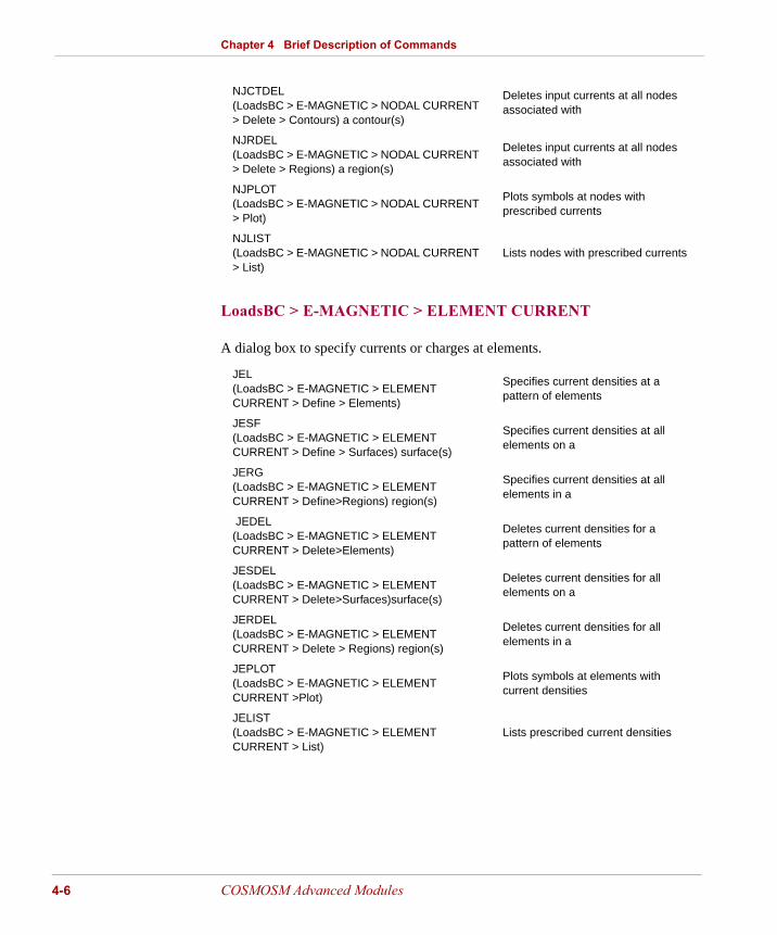
LoadsBC > E-MAGNETIC > ELEMENT CURRENT
A dialog box to specify currents or charges at elements.
NJCTDEL(LoadsBC > E-MAGNETIC > NODAL CURRENT > Delete > Contours) a contour(s)
Deletes input currents at all nodes associated with
NJRDEL(LoadsBC > E-MAGNETIC > NODAL CURRENT > Delete > Regions) a region(s)
Deletes input currents at all nodes associated with
NJPLOT(LoadsBC > E-MAGNETIC > NODAL CURRENT > Plot)
Plots symbols at nodes with prescribed currents
NJLIST(LoadsBC > E-MAGNETIC > NODAL CURRENT > List)
Lists nodes with prescribed currents
JEL(LoadsBC > E-MAGNETIC > ELEMENT CURRENT > Define > Elements)
Specifies current densities at a pattern of elements
JESF(LoadsBC > E-MAGNETIC > ELEMENT CURRENT > Define > Surfaces) surface(s)
Specifies current densities at all elements on a
JERG(LoadsBC > E-MAGNETIC > ELEMENT CURRENT > Define>Regions) region(s)
Specifies current densities at all elements in a
JEDEL(LoadsBC > E-MAGNETIC > ELEMENT CURRENT > Delete>Elements)
Deletes current densities for a pattern of elements
JESDEL(LoadsBC > E-MAGNETIC > ELEMENT CURRENT > Delete>Surfaces)surface(s)
Deletes current densities for all elements on a
JERDEL(LoadsBC > E-MAGNETIC > ELEMENT CURRENT > Delete > Regions) region(s)
Deletes current densities for all elements in a
JEPLOT(LoadsBC > E-MAGNETIC > ELEMENT CURRENT >Plot)
Plots symbols at elements with current densities
JELIST(LoadsBC > E-MAGNETIC > ELEMENT CURRENT > List)
Lists prescribed current densities
COSMOSM Advanced Modules

Part 2 ESTAR / Low Frequency Electromagnetic Analysis
LoadsBC > FUNCTION CURVE
A dialog box to control (time, temperature, or B-H) curves.
Analysis Menu
Analysis > ELECTRO MAGNETIC
A dialog box for commands related to Electromagnetic analysis.
CURDEF(LoadsBC > FUNCTION CURVE > Time/Temp Curve)
Defines (time, temperature, or B-H) curves
CURDEL(LoadsBC > FUNCTION CURVE > Del Time/Temp Curve)
Deletes a pattern of previously defined curves
CURLIST(LoadsBC > FUNCTION CURVE > List > Time/Temp)
Lists previously defined curves
MAKE_CYCLIC(LoadsBC > FUNCTION CURVE > Rept > Time/Temp)
Repeats a pattern of time curves
Command (Path) Intended Use
RESTART(Analysis > Restart)
Starts nonlinear problems from the last successful time step
RENUMBER(Analysis > Renumber)
Minimizes bandwidth of the stiffness matrix
DATA_CHECK(Analysis > Data Check)
Checks element groups, material and real constant sets
R_CHECK(Analysis > Run Check)
Checks element's connectivity, aspect ratio, etc.
A_LIST(Analysis > List Analysis Option)
Lists active options for various types of analyses
EM_OUTPUT(Analysis > ELECTRO MAGNETIC > Output Options)
Controls the printing intervals of results and postprocessing options
COSMOSM Advanced Modules 4-7

Chapter 4 Brief Description of Commands
4-8
Results Menu
EM_MODEL(Analysis > ELECTRO MAGNETIC > Conductor Model)
Specifies stationary or uniformly moving conductors
EM_FREQRANG(Analysis > ELECTRO MAGNETIC > Set Range)
Specifies range & increment of frequencies time harmonic analysis
A_MAGNETIC(Analysis > ELECTRO MAGNETIC > Analysis Options)
Specifies the details of the electromagnetic analysis
R_MAGNETIC(Analysis > ELECTRO MAGNETIC > Run EMag Analysis)
Executes the electromagnetic analysis
Command (Path) Intended Use
Results > PLOT
A dialog box to draw the desired plot.
IDRESULT(Results > PLOT > Identify Result)
Displays location and value of the plotted quantity
MAGPLOT(Results > PLOT > ElectroMagnetic)
Plots electromagnetic component previously loaded
Results > LIST
LIST(Results > LIST > Result)
A submenu to list analysis results
MAGLIST(Results > LIST > EMag Result) analysis
Lists quantities related to an electromagnetic
Results > EXTREMES
A dialog box to list extreme values.
MAGMAX(Results > EXTREMES > Min/Max Emag)
Lists extreme values of electromagnetic components
COSMOSM Advanced Modules

5 Detailed Description of Examples
IntroductionTwo typical examples of electromagnetics problem solved by the ESTAR module. A detailed description of the steps required to set up and solve the problem is given.
3D Permanent Magnet With an Air Gap ExampleFor this problem, the solution needs to determine the flux density in a permanent magnet circuit consisting of a permeable core, a permanent magnet, and air gaps as shown in the Figure 5-1.
It is assumed that there is no flux leakage to the air. As shown in the Figure, 5-1 the problem is symmetric and therefore, only one half of the permanent magnet circuit is considered for
Figure 5-1. Geometry of the Permanent Magnet
Air GapThickness = 0.1Permeability = 1
Plane of symmetry
N
S
Ste
el
Ste
el
Steel
MagnetPermeability =
SteelPermeability = 100000Magnet
COSMOSM Advanced Modules 5-1

Chapter 5 Detailed Description of Examples
5-2
analysis. Figure 5-2 shows the geometry of the circuit along with labels for different dimensions. Note that at the plane of symmetry, the magnetic potentials will be set to zero to ensure the orthogonality of the flux lines. The air gap will be modeled using solid elements with appropriate material properties describing the magnetic permeability of air.
The geometric and material properties for this problem are as shown below:
L = 3 cm
t = 1 cm
H = 3 cm
a = 0.1 cm
Relative permeability of air = 1
Relative permeability of iron = 1 x 10⁵
Coercive force vector Hc = (1885i, 0j, 0k) Oe
Relative permeability of magnet (Br / Hc) = 5.30504
All relevant steps for building and solving this problem are completely described and illustrated in the following paragraphs. As mentioned earlier under notations, all computer prompts are shown in the LIGHT type, and the input or command you need to furnish are shown in BOLD. If you do not see an input shown in bold type against a prompt, simply hit the return key or press the left mouse button once in the display area of GEOSTAR screen.
GEOSTAR provides various geometry construction and manipulation features such as sweeping, dragging, extrusion, regeneration, and many others. To construct the geometry of the permanent magnet, we will first draw a plane rectangular area and extrude it along the required axes to obtain the 3D solid.
You need to first define a plane where the rectangular area is to be drawn. In the figure showing the problem geometry for analysis (shown on the previous page), you can notice that the rectangular cross section at the coordinate axes lies in the Y-Z plane. To start with, you need to construct this rectangular area.
We will input the four corner points of the rectangular area, using the PT (Geometry > POINTS > Define) command shown below successively:
L/2
t
a (air gap)
t
H
t
Figure 5-2. Problem Geometry for Analysis
COSMOSM Advanced Modules

Part 2 ESTAR / Low Frequency Electromagnetic Analysis
PT,1,0,0,-0.5PT,2,0,0,0.5PT,3,0,1,0.5PT,4,0,1,-0.5
The points created above will be used to define a surface. Use the Auto scale icon to view the points created. From the Geometry > SURFACES menu tree, select the SF4PT (Define by 4 Pt) command and input the keypoints 1 through 4 as illustrated below:
Control Panel: Geometry > SURFACES > Define by 4 Pt (SF4PT)Surface > 1Keypoint 1 > 1Keypoint 2 > 2Keypoint 3 > 3Keypoint 4 > 4Underlying surface > 0
The use of SF4PT (Geometry > SURFACES > Define by 4 Pt) command results in the creation of four curves and a surface as shown in the Figure 5-3. To see the labels of entities generated, you may use the Status 1 table.
Surface labeled 1 generated above will be now extruded in the positive X-direction by 1.5 units (equal to the dimension L/2 of the permanent magnet) to form a volume, using the command VLEXTR (Geometry > VOLUMES > GENERATION MENU > Extrusion). The extrusion process also results in the creation of new surfaces, and one of these surfaces can be extruded along the Y axis to form the vertical solid volume of the model. The prompts and input for the VLEXTR (Geometry > VOLUMES > GENERATION MENU > Extrusion) command are illustrated below:
Control Panel: Geometry > VOLUMES > GENERATION MENU > Extrusion (VLEXTR)
Beginning surface > 1Ending surface > 1Increment > 1Axis symbol > XValue > 1.5
Figure 5-3. Rectangular Area for Extrusion
COSMOSM Advanced Modules 5-3

Chapter 5 Detailed Description of Examples
5-4
The VLEXTR (Geometry > VOLUMES > GENERATION MENU > Extrusion) command executed above creates a volume with label 1 as well as five additional surfaces as shown in the Figure 5-4. In order to obtain the view shown in this figure, you need to rescale the image using the Auto scale icon.
Surface 2 which is directly opposite to surface 1 will be further extruded in the X-direction by 1 unit (equal to the thickness “t”), as illustrated below:
Control Panel: Geometry > VOLUMES > GENERATION MENU > Extrusion (VLEXTR)
Beginning surface > 2Ending surface > 2Increment > 1Axis symbol > XValue > 1
Use the Auto scale icon to obtain a clear view of the newly created geometric entities. Surface 10 created by executing the VLEXTR (Geometry > VOLUMES > GENERATION MENU > Extrusion) command above will now be extruded in the Y-direction by 2 units as illustrated below:
Control Panel: Geometry > VOLUMES > GENERATION MENU > Extrusion (VLEXTR)
Beginning surface > 10Ending surface [10] > 10Increment > 1Axis symbol > YValue > 2
Again, use the Auto scale icon to see the updated geometry. You need to continue extruding in the Y-direction to model the air gap as illustrated below:
Figure 5-4. Extrusion of Surface 1
COSMOSM Advanced Modules

Part 2 ESTAR / Low Frequency Electromagnetic Analysis
Control Panel: Geometry > VOLUMES > GENERATION MENU > Extrusion (VLEXTR)
Beginning surface > 12Ending surface > 12Increment > 1Axis symbol > YValue > 0.1
To build the solid volume above the air gap, again issue the VLEXTR (Geometry > VOLUMES > GENERATION MENU > Extrusion) command as illustrated below:
Control Panel: Geometry > VOLUMES > GENERATION MENU > Extrusion (VLEXTR)
Beginning surface > 17Ending surface > 17Increment > 1Axis symbol > YValue > 1
Use the Auto scale icon once again to obtain a clear view of the model built so far. In the last step of extrusion, you need to extrude surface 23 by 1.5 units in the negative X-direction as illustrated below:
Control Panel: Geometry > VOLUMES > GENERATION MENU > Extrusion (VLEXTR)
Beginning surface > 23Ending surface > 23Increment > 1Axis symbol > XValue > -1.5
Change the view to a different orientation by using the View icon (Binocular). You need to select the last icon and provide the viewing coordinates at 1, 2, 3 in the global Cartesian system. The Figure 5-5 shows the geometry of the model constructed using the extrusion process. The figure also shows all keypoints, curves, surfaces, and
Figure 5-5. Generated Keypoints, Curves, Surfaces and Volumes
COSMOSM Advanced Modules 5-5

Chapter 5 Detailed Description of Examples
5-6
volumes generated. Recall that you only input 4 keypoints to start with and the rest were all automatically generated.
You can look at the generated keypoints, curves, surfaces, and volumes by using the respective plotting commands. For example, to see the plot of surfaces, you need to use the command SFPLOT (Edit > PLOT > Surfaces). Similarly, you can use the VLPLOT (Edit > PLOT > Volumes) command to see the volumes generated. Remember to clear the screen using the Clear icon before you issue the plotting commands. Figure 5-6 shows the generated surface and volume plots of the permanent magnet circuit.
Figure 5-6. Surface and Volume Plot
With the geometry of the model fully constructed, you can now proceed to defining the material properties and the type of element to be used in the analysis.
Select the EGROUP (Propsets > Element Group) command to specify the element type for analysis. In the extensive element library of COSMOSM, each element type is assigned a unique name which can be found in on-line help (as well as Chapter 4 of the User Guide) for the EGROUP (Propsets > Element Group) command. For this problem, the 8-node brick element designated as MAG3D is selected, as illustrated below:
Control Panel: Propsets > Element Group (EGROUP)Element group > 1Element category > VolumeElement type (for volume) > MAG3DOP1:virtual displ:0=fixed;1=movable >
Accept defaults ...
COSMOSM Advanced Modules

Part 2 ESTAR / Low Frequency Electromagnetic Analysis
If you issue the command EGLIST (Edit > LIST > Element Groups), the element group defined above will be listed with all the options chosen for the MAG3D element.
The material properties are defined next. For this problem, there are three different material properties (for the magnet, the steel core, and the air gap). In COSMOSM, each material type needs to be assigned a property set number (which can be associated with one or more element groups and section property sets) and you can then input the material properties for that set number. At any time during model development, only one property set number remains active, and you can switch between set numbers and make a different set number active by using the command ACTSET (Control > ACTIVATE > Set Entity), illustrated a little later. Note that the ACTSET (Control > ACTIVATE > Set Entity) command also allows you to switch between various sets such as coordinate sets, real constant (section property) sets, element group numbers and many others. During mesh generation, the active set numbers are associated with the generated elements.
For this problem, material set number 1 is assigned for the permanent magnet, set number 2 for the steel core, and set number 3 for the air gap.
To start with, the properties of the permanent magnet (set number 1) will be described. Select the MPROP (Propsets > Material Property) command and specify MPERM to describe the magnetic permeability, as illustrated below (as before, you can use the on-line help to look up the valid property names):
Control Panel: Propsets > Material Property (MPROP)Material property set > 1 Material property name > MPERMProperty value > 5.30504Material property name > PMAGXProperty value > 1885
Use the command MPLIST (Edit > LIST > Material Props) to list the properties defined above. Note that the letter A is used to designate the active material property set number in the listing.
Clear the screen using Clear icon and issue VLPLOT (Edit > PLOT > Volumes) command to plot the generated volumes. With the properties of the permanent magnet (volume label 1) completely described, you can now proceed to meshing. The generated mesh will have elements associated with element group number 1 (MAG3D elements) and material property set number 1 (defined above for the permanent magnet). Select the M_VL (Meshing > PARAMETRIC MESH >
COSMOSM Advanced Modules 5-7

Chapter 5 Detailed Description of Examples
5-8
Volumes) command. When you use this command, you will be prompted for the number of elements along the first, second and third curves of the volume. This information is necessary to make sure that you generate elements in the adjacent volumes to match for compatibility. The numbering of the three curves in a volume depends on its orientation, and to help you identify them, these curves will be highlighted individually at the respective prompt. The M_VL (Meshing > PARAMETRIC MESH > Volumes) command and its input are illustrated below:
Control Panel: Meshing > PARAMETRIC MESH > Volumes (M_VL)Beginning volume > 1Ending volume > 1Increment > 1 Number of nodes per element > 8
Number of elements on first curve > 2
Watch screen for this curve
Number of elements on second curve > 2 Number of elements on third curve > 4
Spacing ratio for first curve > 1Spacing ratio for second curve > 1 Spacing ratio for third curve > 1
Figure 5-7 shows the generated finite element mesh for the permanent magnet. If you use the command ELIST (Edit > LIST > Elements) you will see that the generated elements are associated with material property set number 1, element group number 1 and the real constant (section property) set number 1. For solid elements, the section property data is not required to be input.
Next, we will proceed to meshing a part of the steel core. You need to first define the material properties of the steel core, using the MPROP (Propsets > Material Property) command. The steel core will be assigned with material property set number 2. However, the element group number will remain the same, as the same type of elements are used throughout the model.
Control Panel: Propsets > Material Property (MPROP)Material property set > 2Material property name > MPERMProperty value > 100000
Figure 5-7. Generated Finite Element Mesh of the Permanent Magnet
COSMOSM Advanced Modules
Part 2 ESTAR / Low Frequency Electromagnetic Analysis
Since a new material property set number was defined, it is the current active material set, and you do not need to activate it using the ACTSET (Control > ACTIVATE > Set Entity) command. On the other hand, if you now had to make material set number 1 active, you would need to use the ACTSET (Control > ACTIVATE > Set Entity) command
Clear the screen using the Clear icon and issue VLPLOT (Edit > PLOT > Volumes) command. To mesh volume 2, type the command M_VL (Meshing > PARAMETRIC MESH > Volumes) as illustrated below:
Control Panel: Meshing > PARAMETRIC MESH > Volumes (M_VL)Beginning volume > 2Ending volume > 1
Accept defaults...
Volume 3 which describes a part of the steel core will be now meshed using the M_VL (Meshing > PARAMETRIC MESH > Volumes) command as illustrated below:
Control Panel: Meshing > PARAMETRIC MESH > Volumes (M_VL)Beginning volume > 3Ending volume > 3Increment > 1 Number of nodes per element > 8Number of elements on first curve > 2Number of elements on second curve > 2Number of elements on third curve > 4
Accept defaults...
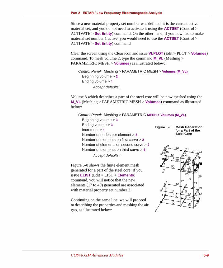
Figure 5-8 shows the finite element mesh generated for a part of the steel core. If you issue ELIST (Edit > LIST > Elements) command, you will notice that the new elements (17 to 40) generated are associated with material property set number 2.
Continuing on the same line, we will proceed to describing the properties and meshing the air gap, as illustrated below:
Figure 5-8. Mesh Generation for a Part of the Steel Core
COSMOSM Advanced Modules 5-9

Chapter 5 Detailed Description of Examples
5-10
Control Panel: Propsets > Material Property (MPROP)Material property set > 3Material property name > MPERMProperty value > 1
Use the command M_VL (Meshing > PARAMETRIC MESH > Volumes) on Volume 4 to mesh the volume describing the air gap with default options. Figure 5-9 shows an enlarged view of the elements in the air gap. The commands Zoomin and Zoomout icons can be used to obtain enlarged or normal views of a model, respectively.
Before meshing the remaining parts of the steel core, you need to first activate the corresponding material set number. The current active material set number is 3 (for the air gap), and you need to make material set number 2 (for the steel core) active by using the ACTSET (Control > ACTIVATE > Set Entity) command as illustrated below:
Control Panel: Control > ACTIVATE > Set Entity (ACTSET)Set label > MPMaterial set number > 2
You can now proceed to meshing the remaining volumes (labeled 5 and 6) as illustrated below:
Control Panel: Meshing > PARAMETRIC MESH > Volumes (M_VL)Beginning volume > 5Ending volume > 5
Accept defaults ...
Control Panel: Meshing > PARAMETRIC MESH > Volumes (M_VL)Beginning volume > 6Ending volume > 6Increment > 1 Number of nodes per element > 8
Figure 5-9. Enlarged View of the Elements in the Air Gap
COSMOSM Advanced Modules

Part 2 ESTAR / Low Frequency Electromagnetic Analysis
Number of elements on first curve > 2
Number of elements on second curve > 2
Number of elements on third curve > 4Accept defaults ...
Clear the screen and issue EPLOT (Edit > PLOT > Elements) command to view the generated finite element mesh. You can use the commands HIDDEN (Display > DISPLAY OPTION > Hidden Element Plot) and EPLOT (Edit > PLOT > Elements) to see a plot of the mesh without the hidden lines. Experiment with other options by using commands such as SHADE, SHRINK (Display > DISPLAY OPTION > Shaded Element Plot, Shrink), etc., to see various views of the mesh generated. The figure below shows the generated finite element mesh with and without the hidden lines.
Figure 5-10. Finite Element Mesh With and Without Hidden Lines
To completely describe the finite element model of the permanent magnet before proceeding to analysis, you need to define the boundary conditions and loads. In GEOSTAR, the loads and constraints can be defined at individual nodes and elements, or directly at the geometric entity level which results in faster model development.
We will first input the boundary conditions at the plane of symmetry. Clear the screen and issue SFPLOT (Edit > PLOT > Surfaces) command to plot the surfaces. You will notice that surfaces 1 and 27 lie in the plane of symmetry. On these surfaces, the magnetic potential needs to be set to zero, in order to ensure the orthogonality of the flux lines. Select the NPSF (LoadsBC > E-MAGNETIC >
COSMOSM Advanced Modules 5-11
Chapter 5 Detailed Description of Examples
5-12
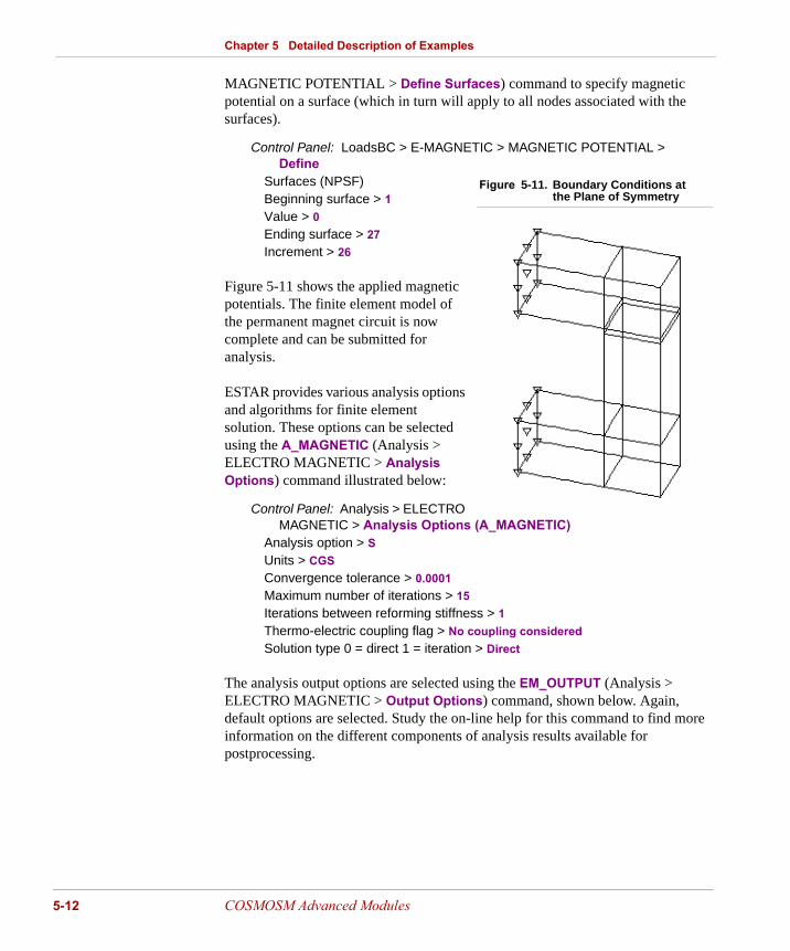
MAGNETIC POTENTIAL > Define Surfaces) command to specify magnetic potential on a surface (which in turn will apply to all nodes associated with the surfaces).
Control Panel: LoadsBC > E-MAGNETIC > MAGNETIC POTENTIAL > Define
Surfaces (NPSF)Beginning surface > 1Value > 0Ending surface > 27Increment > 26
Figure 5-11 shows the applied magnetic potentials. The finite element model of the permanent magnet circuit is now complete and can be submitted for analysis.
ESTAR provides various analysis options and algorithms for finite element solution. These options can be selected using the A_MAGNETIC (Analysis > ELECTRO MAGNETIC > Analysis Options) command illustrated below:
Control Panel: Analysis > ELECTRO MAGNETIC > Analysis Options (A_MAGNETIC)
Analysis option > S Units > CGSConvergence tolerance > 0.0001Maximum number of iterations > 15 Iterations between reforming stiffness > 1Thermo-electric coupling flag > No coupling considered Solution type 0 = direct 1 = iteration > Direct
The analysis output options are selected using the EM_OUTPUT (Analysis > ELECTRO MAGNETIC > Output Options) command, shown below. Again, default options are selected. Study the on-line help for this command to find more information on the different components of analysis results available for postprocessing.
Figure 5-11. Boundary Conditions at the Plane of Symmetry
COSMOSM Advanced Modules

Part 2 ESTAR / Low Frequency Electromagnetic Analysis
Control Panel: Analysis > ELECTRO MAGNETIC > Output Options (EM_OUTPUT)
Magnetic field info flag 0=No N=steps > 1 Post processing info flag > No
As the finite element mesh for each volume was generated independently, there will be duplicate nodes at the common boundaries. These nodes have to be merged, in order to satisfy compatibility requirements. If you forget to execute this step, the program will warn you of a singular stiffness matrix and may abort the solution. Select the NMERGE (Meshing > NODES > Merge) command and accept all default options, as shown below:
Control Panel: Meshing > NODES > Merge (NMERGE)Beginning node > 1 Ending node > 216
Accept defaults ...
Next, select the NCOMPRESS (Edit > COMPRESS > Nodes) command to remove gaps in node numbering.
Control Panel: Edit > COMPRESS > Nodes (NCOMPRESS)Beginning node > 1Ending node > 216Increment > 1
If you now issue the NLIST (Edit > LIST > Nodes) command, the nodes listed will be consecutive.
The finite element model can now be submitted for analysis using the command R_MAGNETIC (Analysis > ELECTRO MAGNETIC > Run EMag Analysis). After the analysis is completed, the control returns to the GEOSTAR screen and you can now proceed with postprocessing. The analysis results are written to a file (jobname.OUT). You can list or print this file to inspect the numerical results. However, it is more plausible to use the powerful postprocessing features of GEOSTAR to study the results on the screen.
To view the resultant magnetic flux, issue the commands ACTMAG, MAGPLOT (or select Results > PLOT > ElectroMagnetic). First, we will look at a contour plot of the flux selected by accepting all default options. The use of ACTMAG, MAGPLOT commands or (Results > PLOT > ElectroMagnetic) is shown below:
COSMOSM Advanced Modules 5-13
Chapter 5 Detailed Description of Examples
5-14
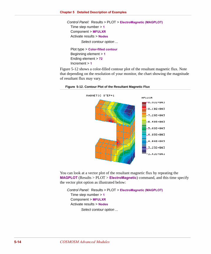
Control Panel: Results > PLOT > ElectroMagnetic (MAGPLOT)Time step number > 1Component > MFULXRActivate results > Nodes
Select contour option ...
Plot type > Color-filled contour Beginning element > 1Ending element > 72Increment > 1
Figure 5-12 shows a color-filled contour plot of the resultant magnetic flux. Note that depending on the resolution of your monitor, the chart showing the magnitude of resultant flux may vary.
Figure 5-12. Contour Plot of the Resultant Magnetic Flux
You can look at a vector plot of the resultant magnetic flux by repeating the MAGPLOT (Results > PLOT > ElectroMagnetic) command, and this time specify the vector plot option as illustrated below:
Control Panel: Results > PLOT > ElectroMagnetic (MAGPLOT)Time step number > 1Component > MFULXRActivate results > Nodes
Select contour option ...
COSMOSM Advanced Modules

Part 2 ESTAR / Low Frequency Electromagnetic Analysis
Plot type > Vector (?) Beginning element > 1Ending element > 72Increment > 1
Figure 5-13 shows a vector plot of the resultant magnetic flux. The boundaries of the permanent magnet circuit were superimposed by using the commands EVAL_BOUND, BOUNDARY (Display > DISPLAY OPTION > Eval Element Bound, Set Bound Plot).
Figure 5-13. Vector Plot of the Resultant Magnetic Flux
At this stage you can also look at the isosurface by the ISOPLOT (Results > PLOT > ElectroMagnetic) command illustrated below.
Control Panel: Results > PLOT > ElectroMagnetic (ISOPLOT)Time step number > 1Component > MFULXRActivate results > Nodes
Select iso plot option ...Number of iso planes > 1
Twelve isoplanes are shown in the Figure 5-14.
COSMOSM Advanced Modules 5-15
Chapter 5 Detailed Description of Examples
5-16
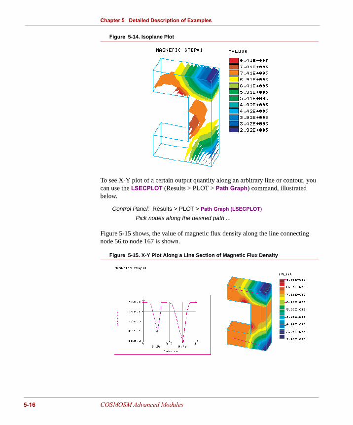
Figure 5-14. Isoplane Plot
To see X-Y plot of a certain output quantity along an arbitrary line or contour, you can use the LSECPLOT (Results > PLOT > Path Graph) command, illustrated below.
Control Panel: Results > PLOT > Path Graph (LSECPLOT)Pick nodes along the desired path ...
Figure 5-15 shows, the value of magnetic flux density along the line connecting node 56 to node 167 is shown.
Figure 5-15. X-Y Plot Along a Line Section of Magnetic Flux Density
COSMOSM Advanced Modules
Part 2 ESTAR / Low Frequency Electromagnetic Analysis
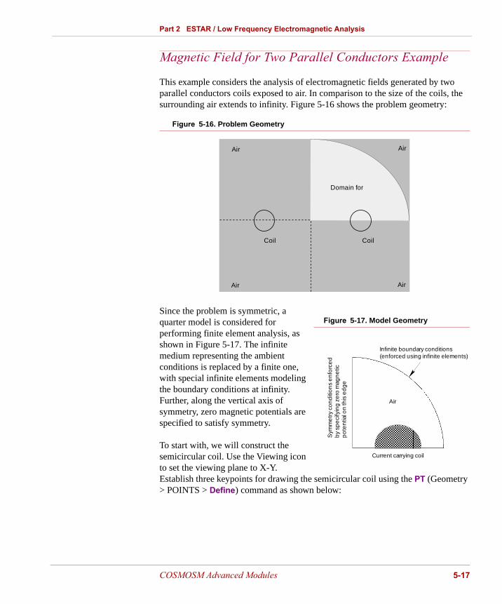
Magnetic Field for Two Parallel Conductors Example
This example considers the analysis of electromagnetic fields generated by two parallel conductors coils exposed to air. In comparison to the size of the coils, the surrounding air extends to infinity. Figure 5-16 shows the problem geometry:
Figure 5-16. Problem Geometry
Since the problem is symmetric, a quarter model is considered for performing finite element analysis, as shown in Figure 5-17. The infinite medium representing the ambient conditions is replaced by a finite one, with special infinite elements modeling the boundary conditions at infinity. Further, along the vertical axis of symmetry, zero magnetic potentials are specified to satisfy symmetry.
To start with, we will construct the semicircular coil. Use the Viewing icon to set the viewing plane to X-Y. Establish three keypoints for drawing the semicircular coil using the PT (Geometry > POINTS > Define) command as shown below:
Air
Coil Coil
Air
AirAir
Domain for
Figure 5-17. Model Geometry
Infinite boundary conditions(enforced using infinite elements)
Current carrying coil
Sym
me
try
con
diti
on
s e
nfo
rce
d
by
spe
cify
ing
ze
ro m
agn
etic
p
ote
ntia
l on
this
ed
ge
Air
COSMOSM Advanced Modules 5-17

Chapter 5 Detailed Description of Examples
5-18
Control Panel: Geometry > POINTS > Define (PT)Keypoint > 1XYZ-coordinate value > 0.002, 0, 0
Control Panel: Geometry > POINTS > Define (PT)Keypoint > 2XYZ-coordinate value > 0.006, 0, 0
Control Panel: Geometry > POINTS > Define (PT)Keypoint > 3XYZ-coordinate value > 0.004, 0.002
The three keypoints defined above will be connected together by an arc using the command CRARC3PT (Geometry > CURVES > CIRCLES > by 3 Points) menu tree, illustrated below:
Control Panel: Geometry > CURVES > CIRCLES > by 3 Points (CRARC3PT)
Curve > 1 Keypoint at one end > 1Keypoint at other end > 2Keypoint on the curve > 3
If you issue ACTNUM,CR,1 and ACTNUM,PT,1 (Control > ACTIVATE > Entity Label) commands (to activate plotting of labels) and then the SCALE (Auto scale icon) command, the following view will be obtained:
Figure 5-18. Construction of Semicircular Arc for the Coil
To construct the outer arc, you need to define three more keypoints as illustrated below (note that keypoint 4 is automatically generated by the program at the center of the circle shown in Figure 5-18):
COSMOSM Advanced Modules
Part 2 ESTAR / Low Frequency Electromagnetic Analysis
Control Panel: Geometry > POINTS > Define (PT)Keypoint > 5XYZ-coordinate value > 0.008, 0, 0
Control Panel: Geometry > POINTS > Define (PT)Keypoint > 6XYZ-coordinate value > 0, 0.008, 0
Control Panel: Geometry > POINTS > Define (PT)Keypoint > 7XYZ-coordinate value > 0, 0, 0
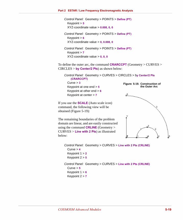
To define the outer arc, the command CRARCCPT (Geometry > CURVES > CIRCLES > by Center/2 Pts) as shown below:
Control Panel: Geometry > CURVES > CIRCLES > by Center/2 Pts (CRARCCPT)
Curve > 3Keypoint at one end > 5Keypoint at other end > 6Keypoint at center > 7
If you use the SCALE (Auto scale icon) command, the following view will be obtained (Figure 5-19):
The remaining boundaries of the problem domain are linear, and are easily constructed using the command CRLINE (Geometry > CURVES > Line with 2 Pts) as illustrated below:
Control Panel: Geometry > CURVES > Line with 2 Pts (CRLINE)Curve > 4Keypoint 1 > 2Keypoint 2 > 5
Control Panel: Geometry > CURVES > Line with 2 Pts (CRLINE)Curve > 5Keypoint 1 > 6Keypoint 2 > 7
Figure 5-19. Construction of the Outer Arc
COSMOSM Advanced Modules 5-19

Chapter 5 Detailed Description of Examples
5-20
Control Panel: Geometry > CURVES > Line with 2 Pts (CRLINE)Curve > 6Keypoint 1 > 7Keypoint 2 > 1
If you clear the screen and execute CRPLOT (Edit > PLOT > Curves) command, the following view will be obtained:
As shown in Figure 5-20, the air surrounding the coil is designated as region 2, and the coil as region 1. In order to generate the finite element mesh in these regions, you need to first define their contours using the CT (Geometry > CONTOURS > Define) command. We will first define the contour of the conductor with bordering curves 1, 2, and 7 as follows:
Control Panel: Geometry > CONTOURS > Define (CT)Contour > 1Mesh flag > Esize
Average element size > 0.0005Number of reference boundary curves > 3
Curve 1 > 1Curve 2 > 2Curve 3 > 7
The contour defined above will be next defined as a region entity using the RG (Geometry > REGIONS > Define) command as illustrated bellow:
Control Panel: Geometry > REGIONS > Define (RG)Region > 1Number of contours > 1
Outer contour > 1Underlying surface > 0
Region 1 representing the coil can now be meshed using the MA_RG (Meshing > AUTO MESH > Regions) command as illustrated below:
Region #2
Region #1
Figure 5-20. Boundary Curves of the Model
COSMOSM Advanced Modules

Part 2 ESTAR / Low Frequency Electromagnetic Analysis
Control Panel: Meshing > AUTO MESH > Regions (MA_RG)Beginning region > 1Ending region > 1Increment > 1Number of smoothing iterations > 2Method > Sweeping
Next, you can proceed to meshing region 2 representing the surrounding air. Instead of using the CT (Geometry > CONTOURS > Define) command (which assigns uniform element size on all border curves), we will use CTNU (Geometry > CONTOURS > Non-Uniform Ct) which will enable you to specify different number of elements along each border curve. Care must be taken to see that the same number of elements are specified on the common boundary curves (1 and 2) in order to have compatible elements. The CTNU (Geometry > CONTOURS > Non-Uniform Ct) command and its input are illustrated below:
Control Panel: Geometry > CONTOURS > Non-Uniform Ct (CTNU)Contour > 2Number of boundary curves [4] > 6
Boundary curve 1 > 1Number of elements on the curve > 7Boundary curve 2 > 2Number of elements on the curve > 7Boundary curve 3 > 4Number of elements on the curve > 4Boundary curve 4 > 3Number of elements on the curve > 11Boundary curve 5 > 5Number of elements on the curve > 8Boundary curve 6 > 6Number of elements on the curve > 4
You can next proceed to defining contour 2 as a region entity and mesh it as illustrated below:
Control Panel: Geometry > REGIONS > Define (RG)Region > 2Number of contours > 1
Outer contour > 2Underlying surface > 0
COSMOSM Advanced Modules 5-21

Chapter 5 Detailed Description of Examples
5-22
Control Panel: Meshing > AUTO MESH > Regions (MA_RG)Beginning region > 2Ending region > 2Increment > 1Number of smoothing iterations > 2Method > Sweeping
Figure 5-21 shows the generated finite element mesh. By default, automatic meshing scheme in COSMOSM generates triangular elements which can be changed to quadrilaterals using the MARGCH (Meshing > AUTO MESH > Region Mesh Type) command.
Select the MARGCH (Meshing > AUTO MESH > Region Mesh Type) command to change the generated elements to quadrilaterals as illustrated below:
Control Panel: Meshing > AUTO MESH > Region Mesh Type (MARGCH)Beginning region > 1Ending region > 2Increment > 1Element type > Q
Total element nodes > 4
Associated element group > 1Shape factor > 0.4Quad elem flag > MixedNumber of smoothing iterations if all quad > 3
Note that some elements may remain as triangles due to the problem geometry. Figure 5-22 shows the modified finite element mesh:
Since triangular elements were used for mesh generation, each quadrilateral element is internally labeled using two triangular elements, each having a unique element number. However, only one label is needed for numbering a quadrilateral element, and you can eliminate the other label. To accomplish this, use the command ECOMPRESS (Edit > COMPRESS > Elements) as illustrated below:
Figure 5-21. Generated Finite Ele
Figure 5-22. Modified Mesh With Quadrilateral (and Some Tri
COSMOSM Advanced Modules

Part 2 ESTAR / Low Frequency Electromagnetic Analysis
Control Panel: Edit > COMPRESS > Elements (ECOMPRESS)Beginning element > 1Ending element > 228Increment > 1Number of elements compressed > 84
Clear the screen and execute the CRPLOT (Edit > PLOT > Curves) command. You can next proceed to applying loads and boundary conditions for this problem. We will first define the current density in the coil. Select the command JERG (LoadsBC > E-MAGNETIC > ELEMENT CURRENT > Define Regions) to define current densities for all elements in region 1 as illustrated below:
Control Panel: LoadsBC > E-MAGNETIC > ELEMENT CURRENT > Define Regions (JERG)
Beginning region > 1Value > 79577Ending region > 1Increment > 1
Since the flux lines will be parallel to the vertical axis of symmetry, you need to impose zero magnetic potentials along this axis (curve 5) using the command NPCR (LoadsBC > E-MAGNETIC > MAGNETIC POTENTIAL > Define Curves) (which applies specified magnetic potentials at all nodes associated with a curve).
Control Panel: LoadsBC > E-MAGNETIC > MAGNETIC POTENTIAL > Define Curves (NPCR)
Beginning curve > 5Value > 0Ending curve > 5Increment > 1
To define the boundary conditions at infinity, you need to use infinite boundary elements. Select the command BECR (LoadsBC > FLUID FLOW > BOUND EL > Define Curves) to define infinite elements between all nodes associated with curve number 3, illustrated below:
Control Panel: LoadsBC > FLUID FLOW > BOUND EL > Define Curves (BECR)
Beginning curve > 3Ending curve > 3Increment > 1
COSMOSM Advanced Modules 5-23

Chapter 5 Detailed Description of Examples
5-24
Figure 5-23 shows the applied boundary conditions and loads for this problem:
The material properties of the conductor and air are described next. The magnetic permeability of the conductor is assumed to be the same as that of air. Select the command MPROP (Propsets > Material Property) and specify the input as illustrated below:
Control Panel: Propsets > Material Property (MPROP)
Material property set > 1Material property name > MPERMProperty value > 12.566E-7
To specify the type of element to be used in the analysis, use the command EGROUP (Propsets > Element Group) submenu as shown below:
Control Panel: Propsets > Element Group (EGROUP)Element group > 1Element category > AreaElement type (for area) > MAG2D
Accept defaults ...
Since there are two different regions, the mesh for each region is generated independently. The nodes on the common boundary therefore have to be merged to satisfy compatibility requirements. Failure to execute this step may result in the program warning you of a singular stiffness matrix and abort the solution. The NMERGE (Meshing > NODES > Merge) command is illustrated below:
Control Panel: Meshing > NODES > Merge (NMERGE)Beginning node > 1Ending node > 148Increment > 1
Accept defaults ...
Use the NCOMPRESS (Edit > COMPRESS > Nodes) command to remove the gaps in node numbering:
Figure 5-23. Applied Boundary Conditions and Loads
COSMOSM Advanced Modules

Part 2 ESTAR / Low Frequency Electromagnetic Analysis
Control Panel: Edit > COMPRESS > Nodes (NCOMPRESS)Beginning node > 1Ending node > 148Increment > 1Number of nodes compressed = 15
The finite element model of the conductor is now ready for analysis. Select the command A_MAGNETIC (Analysis > ELECTRO MAGNETIC > Analysis Options) to specify the analysis parameters. For this problem, all default options are chosen as illustrated below:
Control Panel: Analysis > ELECTRO MAGNETIC > Analysis Options (A_MAGNETIC)
Analysis option > MagnetostaticUnits > MKSConvergence tolerance > 0.0001Maximum number of iterations > 15Iterations between reforming stiffness > 1Thermo-electric coupling flag > No coupling consideredSolution type > Direct
To perform the analysis, use the command R_MAGNETIC (Analysis > ELECTRO MAGNETIC > Run EMag Analysis). As in the previous problem, the analysis results are written to a file (jobname.OUT). After the analysis is run, you can proceed to postprocessing.
Execute BOUNDARY (Display > DISPLAY OPTION > Set Bound Plot) to disable the display of element boundaries. Use the command MAGPLOT (Results > PLOT > ElectroMagnetic) to plot color-filled contours of the resultant magnetic flux, as illustrated below:
Control Panel: Results > PLOT > ElectroMagnetic (MAGPLOT)Time step number > 1Component > MFULXRActivate results > Nodes
Select contour option ...
Plot type > Color-filled contour Beginning element > 1Ending element > 144Increment > 1
COSMOSM Advanced Modules 5-25

Chapter 5 Detailed Description of Examples
5-26
Figure 5-24 shows the contour plot of the resultant magnetic flux.
Figure 5-24. Contour Plot of the Resultant Magnetic Flux
To see a vector plot of the resultant magnetic flux, repeat the MAGPLOT (Results > PLOT > ElectroMagnetic) command, and this time, specify the vector option as shown below:
Control Panel: Results > PLOT > ElectroMagnetic (MAGPLOT)Time step number > 1Component > MFULXRActivate results > Nodes
Select contour option ...
Plot type > VectorBeginning element > 1Ending element > 144Increment > 1
The Figure 5-25 shows the vector plot of the resultant magnetic flux.
COSMOSM Advanced Modules

Part 2 ESTAR / Low Frequency Electromagnetic Analysis
Figure 5-25. Vector Plot of the Resultant Magnetic Flux
Next, we will also look at the distribution of magnetic potentials. Execute the MAGPLOT (Results > PLOT > ElectroMagnetic) command again, and this time, specify NPOTEN as the component for processing, as illustrated below:
Control Panel: Results > PLOT > ElectroMagnetic (MAGPLOT)Time step number > 1Component > NPOTENActivate results > Nodes
Select contour option ...
Plot type > Color-filled contour Beginning element > 1Ending element > 144Increment > 1
In order to obtain a clear view, it is a good idea to disable the element boundaries before you plot the magnetic potential lines. Select the command BOUNDARY (Display > DISPLAY OPTION > Set Bound Plot) and specify 0 for the first prompt to disable the display of element boundaries. Next, type the MAGPLOT (Results > PLOT > ElectroMagnetic) command and specify the line option as shown below:
COSMOSM Advanced Modules 5-27

Chapter 5 Detailed Description of Examples
5-28
Control Panel: Results > PLOT > ElectroMagnetic (MAGPLOT)Time step number > 1Component > MFULXRActivate results > Nodes
Select contour option ...
Plot type > Vector (?) Beginning element > 1Ending element > 144Increment > 1
Deactivate curve labels using ACTNUM (Control > ACTIVATE > Entity Label) and plot curves 3 through 7 using the command CRPLOT (Edit > PLOT > Curves). Figure 5-26 shows a line plot of the distribution of magnetic potentials.
Figure 5-26. Lines of Equal Magnetic Potentials
COSMOSM Advanced Modules

6 Verification Problems
Introduction
In the following, a comprehensive set of verification problems are provided to illustrate the various features of the electromagnetic analysis module (ESTAR). The problems are selected to cover a wide range of applications in different electromagnetic analyses.
The input files for the verification problems are available in the “...\Vprobs\ Emagnetics” folder. Where “...” denotes the COSMOSM 2.0 folder. For example the input file for problem EM1 is available in the file “...\Vprobs\Emagnetics\ EM1.GEO.”
COSMOSM Advanced Modules 6-1

Chapter 6 Verification Problems
6-2
TYPE: Magnetostatic analysis, axisymmetric “MAG2D” elements.
REFERENCE: Kraus, J. D. “Electromagnetics,” McGraw-Hill Book Company, 1984.
PROBLEM: Obtain the magnetic flux density due to a current loop in the air.
GIVEN: Permeability of air = 4 Π E-7
Radius of the loop R = 0.02 m
Current = 10 amp
MODELING HINT: The infinite extent of the problem is modeled by putting boundary condition A = 0 at boundaries which are sufficiently remote from the current loop.
COMPARISON OF RESULTS:Magnetic flux at the center of the loop x = 0, y = 10 (Node 621):
EM1: Magnetic Field of a Current Loop
Heat Flux (Gauss)
Theory 3.141
COSMOSM 3.1361
Figure EM1-1
R
Z
Y
X
Problem Sketch
Finite Element
X
Y
1641
20 cm
1 4131
168110 cm
821
COSMOSM Advanced Modules

Part 2 ESTAR / Low Frequency Electromagnetic Analysis
TYPE: Magnetostatic analysis, axisymmetric “MAG2D” elements.
REFERENCE: J. L. Coulomb and G. Meunier, “Finite Element Implementation of Virtual Work Principle for Magnetic or Electric Force and Torque Computation,” IEEE Trans. on Magnetics, V20, 1984, pp. 1894-1896.
PROBLEM: Obtain the magnetic forces between two cylindrical coils.
Figure EM2–1
EM2: Magnetic Force Between Two Cylindrical Coils
Problem Sketch
h
d
R2
R1J
550
221X
Y
529
CL
CL
0.2m
0.2
4m
315 316
338337
227
205 206
228
Modeling Domain
Finite Element Model
COSMOSM Advanced Modules 6-3
Chapter 6 Verification Problems
6-4
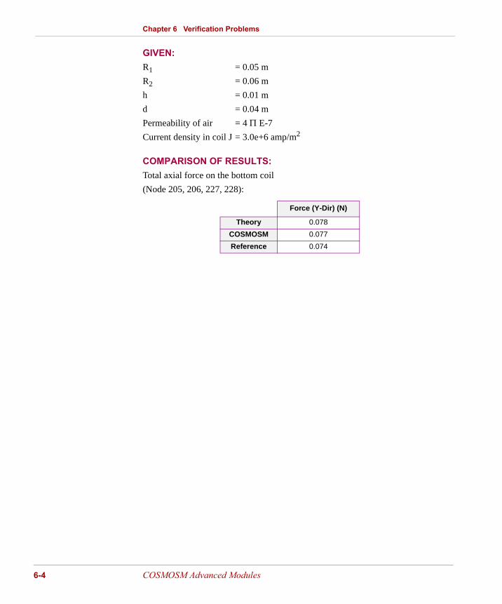
GIVEN: R1 = 0.05 m
R2 = 0.06 m
h = 0.01 m
d = 0.04 m
Permeability of air = 4 Π E-7
Current density in coil J = 3.0e+6 amp/m2
COMPARISON OF RESULTS:Total axial force on the bottom coil
(Node 205, 206, 227, 228):
Force (Y-Dir) (N)
Theory 0.078
COSMOSM 0.077
Reference 0.074
COSMOSM Advanced Modules

Part 2 ESTAR / Low Frequency Electromagnetic Analysis
TYPE: Magnetostatic analysis and force calculation using two different techniques, planar “MAG2D” elements.
REFERENCE:J. L. Coulomb and G. Meunier, “Finite Element Implementation of Virtual Work Principle for Magnetic or Electric Force and Torque Computation,” IEEE Trans. on Magnetics, V20, 1984, pp. 1894-1896.
PROBLEM: Calculate the magnetic force between two parallel coils, using two different techniques
1. Standard Technique (J*B)
2. Virtual Work Technique
EM3: Magnetic Force Between Two Coils (J*B Technique)
Figure EM3-1
Problem Sketch
0.04 m
0.01 m
0.01 m
31
63
651 681
(Case A)
y
354
323 324
355 359
378 379
360
32
1 2 3
ModelingDomain
Finite Element Model
COSMOSM Advanced Modules 6-5

Chapter 6 Verification Problems
6-6
GIVEN: Permeability of air = 4 Π E-7
Current density in coil J = +/- 1.e+6 amp/m2
COMPARISON OF RESULTS:
NOTE:In the standard technique, forces are calculated for all the conductors which includes both left and right hand side coils.
Force (X-Dir) (N)
COSMOSM (Case A) - 0.0349
COSMOSM (Case B) - 0.0351
COSMOSM Advanced Modules

Part 2 ESTAR / Low Frequency Electromagnetic Analysis
TYPE: Magnetostatic analysis, planar “MAG2D” elements.
REFERENCE: O.C. Zienkiewicz, J. Lyness, and D.R.J. Owen, “Three Dimensional Magnetic Field Determination Using a Scalar Potential-A Finite Element Solution,” IEEE Trans. on Magnetics, Vol Mag-13, No. 5, 1977, pp. 1649-1656.
PROBLEM: Obtain the magnetic field for a two dimensional transformer specified below.
Figure EM4–1
EM4: Magnetic Field in a 2D Transformer
16 cm
Problem Sketch Finite Element Model
Conductors
4 cm
16 cm
20 cm
20 cm
.5 cm
A = o
A = o
20 cm
20 cmA = o
AIR
IRON
δA/δn = 0
AIR
4
Y
X
Modeling Domain
COSMOSM Advanced Modules 6-7

Chapter 6 Verification Problems
6-8
GIVEN: Permeability of iron = 4.668810e+003 (CGS)
Current density in coil J = 10 Ab amp/cm2
MODELING HINT: Due to symmetry only a quarter of the transformer needs to be modeled. The necessary Boundary conditions to insure symmetry are shown in the above figure.
COMPARISON OF RESULTS:Magnitude of flux density at x = 1, y = 0.5 (Node 11):
Flux Density in Y-Direction (Tesla)
Reference 2.42
COSMOSM 2.41
COSMOSM Advanced Modules
Part 2 ESTAR / Low Frequency Electromagnetic Analysis
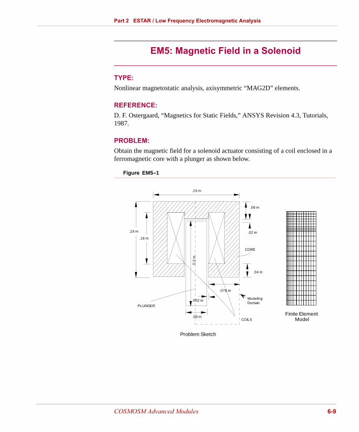
TYPE: Nonlinear magnetostatic analysis, axisymmetric “MAG2D” elements.
REFERENCE: D. F. Ostergaard, “Magnetics for Static Fields,” ANSYS Revision 4.3, Tutorials, 1987.
PROBLEM: Obtain the magnetic field for a solenoid actuator consisting of a coil enclosed in a ferromagnetic core with a plunger as shown below.
Figure EM5–1
EM5: Magnetic Field in a Solenoid
Problem Sketch
Finite Element Model
.24 m
.06 m
.02 m
.04 m
CORE
PLUNGER
.078 m
.002 m
.08 m
.24 m
.16 m
COILS
0.2
m
Modeling Domain
COSMOSM Advanced Modules 6-9

Chapter 6 Verification Problems
6-10
GIVEN: Relative permeability of air and coil = 1
Current density in coil J = 1e+6 amp/m2
B-H curve data for core and plunger:
MODELING HINT: For axisymmetric models, a fine mesh should be used in the radial direction near the center axis to avoid inaccuracy caused by 1/x term in the formulation. Modeling has been done in CGS units.
COMPARISON OF RESULTS:Maximum flux density in the core (Node 311):
B (T) 0.8 95 1.0 1.1-1.15 1.25 1.4 1.55 1.65
H (A/m) 460 640 720 890 -1020 1280 1900 3400 6000
Flux Density in
Y-Direction (Tesla)
Reference 0.933
COSMOSM 0.927
COSMOSM Advanced Modules
Part 2 ESTAR / Low Frequency Electromagnetic Analysis
TYPE: Transient electromagnetic analysis, plane “MAG2D” elements.
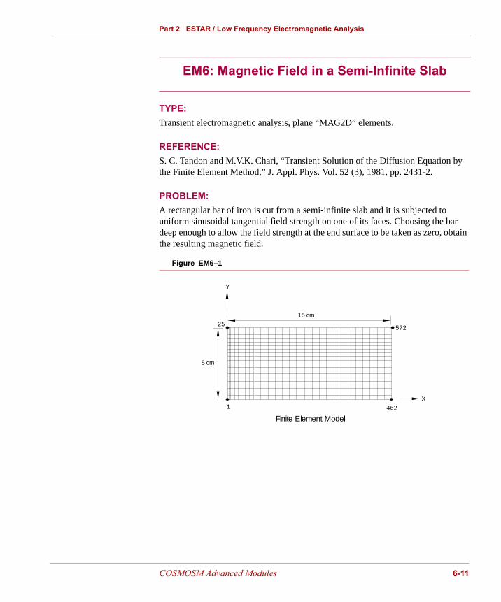
REFERENCE: S. C. Tandon and M.V.K. Chari, “Transient Solution of the Diffusion Equation by the Finite Element Method,” J. Appl. Phys. Vol. 52 (3), 1981, pp. 2431-2.
PROBLEM: A rectangular bar of iron is cut from a semi-infinite slab and it is subjected to uniform sinusoidal tangential field strength on one of its faces. Choosing the bar deep enough to allow the field strength at the end surface to be taken as zero, obtain the resulting magnetic field.
Figure EM6–1
EM6: Magnetic Field in a Semi-Infinite Slab
15 cm
462
572
1
5 cm
Y
X
Finite Element Model
25
COSMOSM Advanced Modules 6-11

Chapter 6 Verification Problems
6-12
GIVEN: H = 500 sin (ωt) A/m
ω = 80 rad/s
Relative permeability = 100
Electric conductivity = 1E+6
MODELING HINT: The tangential field at the right hand side boundary is produced by applying a current sheet of magnitude .5 Ab amp/cm (CGS unit) at the plane x = 0.
COMPARISON OF RESULTS:Field intensity Hy at x = 0 (Node 1) and time = 0.01s:
Field Intensity(Oersted)
Theory 3.69
COSMOSM 3.731
COSMOSM Advanced Modules

Part 2 ESTAR / Low Frequency Electromagnetic Analysis
TYPE: Transient electromagnetic analysis, plane “MAG2D” elements.
REFERENCE: M. A. Jamnia and D. F. Ostergaard, “Magnetics,” ANSYS Revision 4.3, Seminar Notes, 1988.
PROBLEM: This problem consists of a very long hollow aluminum cylinder placed in a uniform magnetic field. Obtain the induced eddy currents when the magnetic field decays exponentially with time.
Figure EM7–1
GIVEN:Relative permeability = 1
Electric conductivity = 2.538E+7 (MKS unit)
By = B0 e−τ / τ
EM7: Eddy Current Analysis of Cylinder in a Decaying Field
Problem Sketch Finite Element Model
y
x
R i
Ro
COSMOSM Advanced Modules 6-13
Chapter 6 Verification Problems
6-14
Where:
B0 = 0.1 Tesla
Τ = 0.0397
Ri = 13.17 cm
Ro = 13.65 cm
MODELING HINT: Due to symmetry only the upper right hand side of the problem is modeled. To set up the initial uniform field, the potential at the x = 78 cm plane is given a value A = -78000 (CGS units are used). Running this problem in the static mode a uniform By = 1000 Gauss is obtained. For the transient response the same problem is run using the uniform field as the initial condition (by activating the RESTART command and transient mode) and varying the boundary values at x = 78 cm exponentially with time.
COMPARISON OF RESULTS:Total eddy current induced in one quarter of the cylinder (currents are in Ab amp).
COSMOSM Advanced Modules

Part 2 ESTAR / Low Frequency Electromagnetic Analysis
TYPE: Nonlinear magnetostatic analysis, plane “MAG2D” element.
REFERENCE:D. F. Ostergaard, “Magnetics for Static Fields,” ANSYS Revision 4.3, Tutorials, 1987.
PROBLEM:Consider an inductor consisting of a ferromagnetic core wound with a coil around one leg of the core. Assuming a 2D model, obtain the magnetic flux and the inductance of the device.
Figure EM8–1
EM8: 2D Inductor with Ferromagnetic Core
15 cm
Finite Element Model
A = o
A = o
1.55 m
1.60 m A = o
Air
30 cm
Problem Sketch
Conductors
10 cm
30 cm
55 cm
Air
2 cm
(Core)
A = o
Air
(Core)
60 cm
X
Y
COSMOSM Advanced Modules 6-15

Chapter 6 Verification Problems
6-16
GIVEN:Relative permeability of air and coil = 1
Current density in coil J = 1e+5 amp/m2
B-H curve data for core:
MODELING HINT: Since the inductor is operating at a point such that the core is highly saturated, it is necessary to model the air in the window and external to the core, in addition to the core itself.
COMPARISON OF RESULTS:Terminal inductance (per unit length)
NOTE:The induction value in the output file has been converted from CGS to MKS unit system.
H (Oersted) 5.7805 6.912 8.042 9.0475 11.1837
B (Gauss) 8000 8800 9500 10000 11000
H (Oersted) 12.8173 16.0844 23.8754 42.7244 75.396
B (Gauss) 11500 12500 14000 15500 16500
H (Oersted) 125.664 251.327 376.991
B (Gauss) 17000 17500 17750
Terminal Inductance(Henries)
Reference 0.5618E-4
COSMOSM 0.5636E-4
COSMOSM Advanced Modules
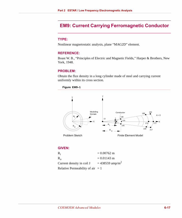
Part 2 ESTAR / Low Frequency Electromagnetic Analysis
TYPE: Nonlinear magnetostatic analysis, plane “MAG2D” element.
REFERENCE: Boast W. B., “Principles of Electric and Magnetic Fields,” Harper & Brothers, New York, 1948.
PROBLEM: Obtain the flux density in a long cylinder made of steel and carrying current uniformly within its cross section.
Figure EM9–1
GIVEN: Ri = 0.00762 m
Ro = 0.01143 m
Current density in coil J = 438559 amp/m2
Relative Permeability of air = 1
EM9: Current Carrying Ferromagnetic Conductor
6
228
170
131
Problem Sketch
Ri
Ro
X
Finite Element Model
Y
A = 0
R
R o
i
Conductor
Y
X
2131
138
145
189190
171
217
ModelingDomain
COSMOSM Advanced Modules 6-17

Chapter 6 Verification Problems
6-18
B-H curve data for the conductor:
MODELING HINT:Due to symmetry only a 5 degree slice of the cylinder is modeled. Part of the external air is also modeled to account for the infinite extend of the problem in the radial direction.
COMPARISON OF RESULTS:Tangential flux density (Nodes 32 and 34)
B(T): 0.21 0.55 0.8 0.95 1.0 1.1 1.15 1.25 1.4
H(A/m): 150 300 460 640 720 890 1020 1280 1900
Tangential Flux Density (Tesla)
r = 0.009525 m r = 0.01795 m
Reference 1.03 1.220
COSMOSM 1.02 1.214
COSMOSM Advanced Modules
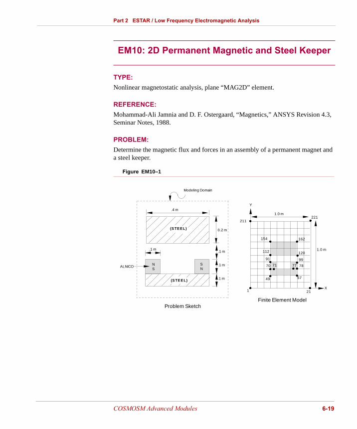
Part 2 ESTAR / Low Frequency Electromagnetic Analysis
TYPE: Nonlinear magnetostatic analysis, plane “MAG2D” element.
REFERENCE:Mohammad-Ali Jamnia and D. F. Ostergaard, “Magnetics,” ANSYS Revision 4.3, Seminar Notes, 1988.
PROBLEM:Determine the magnetic flux and forces in an assembly of a permanent magnet and a steel keeper.
Figure EM10–1
EM10: 2D Permanent Magnetic and Steel Keeper
1.0 m
1.0 m
Problem SketchFinite Element Model
.4 m
.1 m.1 m
.1 m
.1 m
Y
X
(STEEL)
ALNICO
(STEEL)
0.2 m
NS
SN
154
112
91
70
49
162
120
99
78
57
21
71 77
221211
1
Modeling Domain
COSMOSM Advanced Modules 6-19
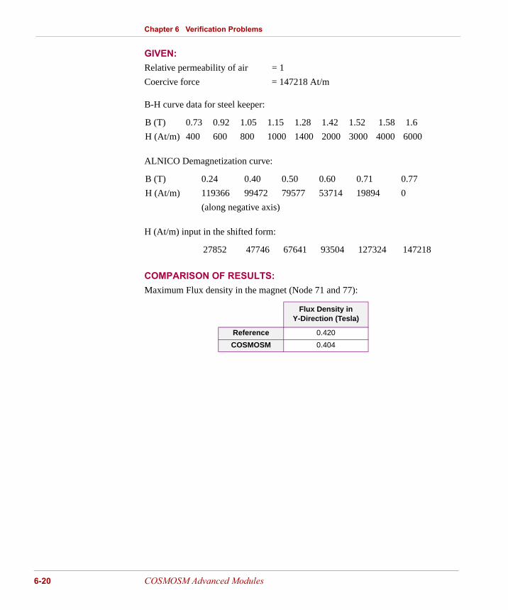
Chapter 6 Verification Problems
6-20
GIVEN:Relative permeability of air = 1
Coercive force = 147218 At/m
B-H curve data for steel keeper:
ALNICO Demagnetization curve:
H (At/m) input in the shifted form:
COMPARISON OF RESULTS:Maximum Flux density in the magnet (Node 71 and 77):
B (T) 0.73 0.92 1.05 1.15 1.28 1.42 1.52 1.58 1.6
H (At/m) 400 600 800 1000 1400 2000 3000 4000 6000
B (T) 0.24 0.40 0.50 0.60 0.71 0.77
H (At/m) 119366 99472 79577 53714 19894 0
(along negative axis)
27852 47746 67641 93504 127324 147218
Flux Density inY-Direction (Tesla)
Reference 0.420
COSMOSM 0.404
COSMOSM Advanced Modules

Part 2 ESTAR / Low Frequency Electromagnetic Analysis
TYPE: Three dimensional magnetostatic analysis, “MAG3D” element.
REFERENCE:Moon, F. C., “Magneto-Solid Mechanics,” John Wiley & Sons, New York, 1984.
PROBLEM: Determine the flux density in a permanent magnet circuit consisting of a permeable core, a permanent magnet and an air gap. Assume that there is no flux leakage to the air.
Figure EM11-1
GIVEN:L = 3 cm
t = 1 cm
H = 3 cm
a = 0.1 cm
EM11: 3D Permanent Magnetic with an Air Gap
Finite Element Model
Problem Sketch
L/2
t
a (air gap)
t
H
t
COSMOSM Advanced Modules 6-21

Chapter 6 Verification Problems
6-22
Relative permeability of air = 1
Relative permeability of iron = 1e+5
Coercive force vector Hc = 1885i, 0j, 0k
Relative permeability of magnet (Br/Hc)= 5.30504
Figure EM11-2
MODELING HINT: Due to symmetry only half of the device is modeled and at the symmetry planes magnetic potentials are set to value zero to insure the orthogonality of the flux lines.
COMPARISON OF RESULTS:Amplitudes of flux density and field intensity:
Permanent Magnet
Air Gap
Flux Density (Gauss) Field Intensity (Oersted)
Theory7387492
73877387
COSMOSM7386493
73877387
H1885 H(oe)
B(G)
B = 1E4r
Magnet's Demagnetization Curve
COSMOSM Advanced Modules

Part 2 ESTAR / Low Frequency Electromagnetic Analysis
TYPE: Electrostatic analysis, “MAG2D” elements.
REFERENCE: R. V. Churchill, et. al., “Complex Variables and Applications,” McGraw-Hill Book Company, 1976, Chapter 9.
PROBLEM: Obtain the electric field due to the prescribed voltages at the edges.
Figure EM12-1
GIVEN:Width = Height = 4 m
Permittivity (dielectric constant) =1E-7 F/m
EM12: Electric Field in a Rectangular Slab
MODELING HINT:
Due to symmetry only the lower half of the plate is modeled using triangular type elements.
COMPARISON OF RESULTS:Voltage at the center, (x = y = 2.)
V (Voltage)
Theory 25.0
COSMOSM 25.0
0
I
Y
0
0
I
X
37
28
19
36
27
18
1
ν = 100
Problem Sketch
38 39 40 41 42 43 44 45
Finite Element Model
Y
X2 3 4 5 6 7 8 9
COSMOSM Advanced Modules 6-23
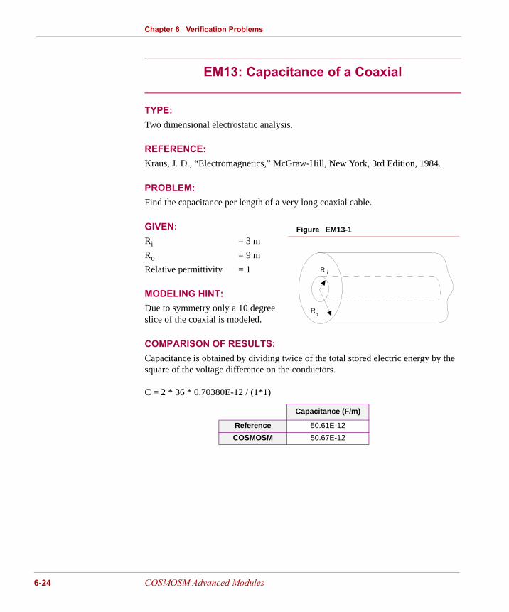
Chapter 6 Verification Problems
6-24
TYPE: Two dimensional electrostatic analysis.
REFERENCE: Kraus, J. D., “Electromagnetics,” McGraw-Hill, New York, 3rd Edition, 1984.
PROBLEM: Find the capacitance per length of a very long coaxial cable.
GIVEN:Ri = 3 m
Ro = 9 m
Relative permittivity = 1
MODELING HINT:Due to symmetry only a 10 degree slice of the coaxial is modeled.
COMPARISON OF RESULTS:Capacitance is obtained by dividing twice of the total stored electric energy by the square of the voltage difference on the conductors.
C = 2 * 36 * 0.70380E-12 / (1*1)
EM13: Capacitance of a Coaxial
Capacitance (F/m)
Reference 50.61E-12
COSMOSM 50.67E-12
Figure EM13-1
R
R
i
o
COSMOSM Advanced Modules

Part 2 ESTAR / Low Frequency Electromagnetic Analysis
TYPE: Three dimensional magnetostatic analysis with current source.
REFERENCE: Boast, W. B., “Principle of Electric and Magnetic Fields,” Harper and Brothers, 1948.
PROBLEM: Calculate the magnetic field intensity and inductance of the following nonferrous solenoid.
GIVEN:L = 0.127 m
R = 0.0127 m
I = 0.5 ampere
Wire diameter = 0.0005486 m
Relative permeability = 1
No. of turns N = 231
No. of turns NI = 115.5 amp-turns
MODELING HINTS:Due to symmetry only upper half of the solenoid is considered, in addition it is only necessary to model a slice of the solenoid. A 10 degree slice is chosen. Since no magnetic material is present the field intensity is totally due to Biot-Savart integral, and potential value is set equal to zero throughout the model. Part of the air surrounding the solenoid is modeled for accurate inductance calculation.
EM14: Inductance of a Solenoid
Figure EM14-1
Y
XR
COSMOSM Advanced Modules 6-25

Chapter 6 Verification Problems
6-26
COMPARISON OF RESULTS: Total inductance = 2 * 36 * 3.3968E-6
Center Flux Density 100*BZ
(Gauss)Reference COSMOSM
Z = 0 1120 1120
Z = .01905 2.12 2.12
Reference COSMOSM
Inductance1E + 4*L(H)
2.46 2.44
COSMOSM Advanced Modules
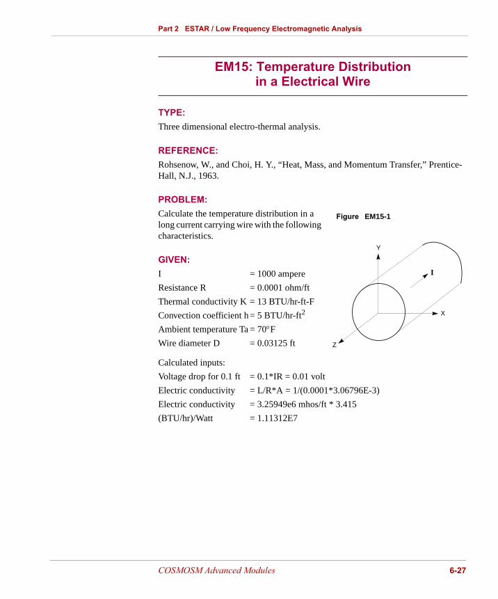
Part 2 ESTAR / Low Frequency Electromagnetic Analysis
TYPE: Three dimensional electro-thermal analysis.
REFERENCE: Rohsenow, W., and Choi, H. Y., “Heat, Mass, and Momentum Transfer,” Prentice-Hall, N.J., 1963.
PROBLEM: Calculate the temperature distribution in a long current carrying wire with the following characteristics.
GIVEN: I = 1000 ampere
Resistance R = 0.0001 ohm/ft
Thermal conductivity K = 13 BTU/hr-ft-F
Convection coefficient h= 5 BTU/hr-ft2
Ambient temperature Ta = 70°F
Wire diameter D = 0.03125 ft
Calculated inputs:
Voltage drop for 0.1 ft = 0.1*IR = 0.01 volt
Electric conductivity = L/R*A = 1/(0.0001*3.06796E-3)
Electric conductivity = 3.25949e6 mhos/ft * 3.415
(BTU/hr)/Watt = 1.11312E7
EM15: Temperature Distribution in a Electrical Wire
Figure EM15-1
Y
X
Z
I
COSMOSM Advanced Modules 6-27

Chapter 6 Verification Problems
6-28
MODELING HINTS: For convenience a 0.1 foot length of the wire is considered and due to axisymmetric nature of the problem a 10 degree slice of the wire is chosen for modeling. Electric conductivity includes the conversion factor 3.415 so that power loss units match the thermal units. For electro-thermal coupling, first current flow analysis is run to calculate the resulting element heat densities and then the heat transfer analysis is done for temperature calculations.
COMPARISON OF RESULTS:
Center Line Temperature °F
Reference 419.9
COSMOSM 418.7
COSMOSM Advanced Modules

Part 2 ESTAR / Low Frequency Electromagnetic Analysis
TYPE: Magneto-structural analysis.
REFERENCE: Moon, F. A., “Magneto-Solid Mechanics,” John Wiley & Sons, New York, 1984, Chapter 4.
PROBLEM: Calculate the magnetic flux density and stress distribution in a long, thick solenoid with a uniform distribution of circumferential current. Assume an isotropic elastic model.
GIVEN:J = 10 Ab amp/cm2
a = 1 cm
b = 2 cm
t = 0.2 cm
E = 0.75E11 dyne/cm
Poisson ratio = 0.33
Relative permeability = 1
MODELING HINTS: Since the solenoid is very long, an infinite axial length is assumed. For convenience a 0.2 cm length of the solenoid is modeled and axial displacement are set equal to zero to produce the infinite-length effect of the model. Furthermore, it is assumed that the magnetic field external to the solenoid is zero and therefore only the axial component of magnetic flux density is non-zero. Dirichlet boundary condition A = 0 at the center r = 0 is imposed and at r = 2 the magnetic potentials are set to be equal. All the other boundaries are automatically subjected to Neumann boundary conditions.
EM16: Stress Distribution in a Long, Thick Solenoid
Figure EM16-1
a
b
Y
X
J
COSMOSM Advanced Modules 6-29
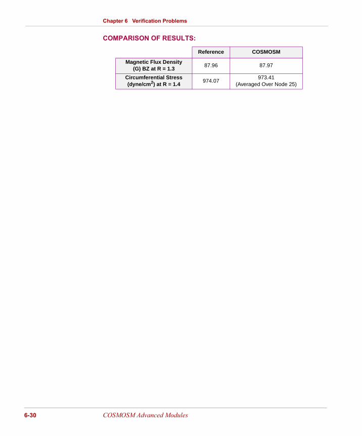
Chapter 6 Verification Problems
6-30
COMPARISON OF RESULTS:
Reference COSMOSM
Magnetic Flux Density(G) BZ at R = 1.3
87.96 87.97
Circumferential Stress(dyne/cm2) at R = 1.4
974.07973.41
(Averaged Over Node 25)
COSMOSM Advanced Modules

Part 2 ESTAR / Low Frequency Electromagnetic Analysis
TYPE: Two dimensional magnetostatic analysis with infinite elements.
REFERENCE: Sergio Pissanetzky, “A Simple Infinite Element,” COMPEL, Vol. 3, No. 2, 1984, pp. 107-114.
PROBLEM: Calculate the magnetic fields due to two parallel conductors surrounded by air.
GIVEN:Current I = 1 amp
Radius of coil R = 0.002 m
Relative permeability = 1
Center distance between two coils D = 0.008 m
MODELING HINTS: Due to symmetry only a quarter model is considered. The infinite medium representing the surrounding air is replaced by a finite one with special infinite elements modeling the boundary conditions at infinity.
COMPARISON OF RESULTS:Magnetic flux densities at y = 0:
EM17: Magnetic Field for Two Parallel Conductors
X = 0.002 X = 0.006
Theory 1.205e-4 0.68e-4
COSMOSM 1.206e-4 0.69e-4
Figure EM17-1
Problem Sketch
Finite Element Model
D
R
COSMOSM Advanced Modules 6-31

Chapter 6 Verification Problems
6-32
Type:Two-dimensional electrostatic analysis with infinite elements.
Reference:Sergio Pissanetzky, “A Simple Infinite Element,” COMPEL, Vol. 3, No. 2, 1984, pp. 107-114.
Problem:Calculate the voltages due to two parallel line charges surrounded by air.
Given:Relative permittivity = 1
Charge density = 0.5
Distance between the charges = 1
Modeling Hints:Due to symmetry only a quarter model is considered. The infinite medium representing the surrounding air is replaced by a finite one with special infinite elements modeling the boundary conditions at infinity.
COMPARISON OF RESULTS:Voltages at:
EM18: Electrostatic Field for Two Line Charge Densities
X = Y = 0.1666 X = Y = 0.5
Analytical Solution 0.0974 0.1281
COSMOSM 0.0976 0.1281
Figure EM18-1
Problem Sketch
Finite Element Model
Infinite Elements
COSMOSM Advanced Modules

Part 2 ESTAR / Low Frequency Electromagnetic Analysis
TYPE: Three dimensional magnetostatic analysis, “TETRA10” element.
REFERENCE:Moon, F. C., “Magneto-Solid Mechanics,” John Wiley & Sons, New York, 1984.
PROBLEM:Determine the flux density in a permanent magnet circuit consisting of a permeable core, a permanent magnet and an air gap. Assume that there is no flux leakage to the air.
GIVEN:L = 3 cm
t = 1 cm
H = 3 cm
a = 0.1 cm
Relative permeability of air = 1
Relative permeability of iron = 1E+5
Coercive force vector Hc = 1885i, 0j, 0k
Relative permeability of magnet (Br/Hc)= 5.30504
EM19: 3D Permanent Magnet with an Air Gap
Figure EM19-1
Problem Sketch Finite Element Model
COSMOSM Advanced Modules 6-33

Chapter 6 Verification Problems
6-34
Figure EM19-2
MODELING HINTS: Due to symmetry only half of the device is modeled and at the symmetry planes magnetic potentials are set to value zero to insure the orthogonality of the flux lines.
COMPARISON OF RESULTS:Amplitudes of flux density and field intensity:
Permanent Magnet
Air Gap
Flux Density (Gauss) Field Intensity (Oersted)
Theory7387492
73877387
COSMOSM7386493
73867386
H1885 H(oe)
B(G)
B = 1E4r
Magnet's Demagnetization Curve
COSMOSM Advanced Modules

Part 2 ESTAR / Low Frequency Electromagnetic Analysis
TYPE:Time harmonic magnetic analysis for an axisymmetric model
REFERENCE:D. Ostergaard, “Magnetics for Time Varying Fields,” ANSYS Revision 4.4, Seminar Notes, 1988.
PROBLEM:For the given cylindrical transformer which consists of two windings, laminated core, yoke, and an outer tank, calculate the power loss due to eddy currents generated in the tank wall assuming the yoke is infinitely permeable.
Figure EM20-1
EM20: Power Loss in a Cylindrical Transformer
Finite Element Model
Problem Sketch
Y (Axial)
X(Radial)
Core
Yoke
.02 m
1.2 m
.17 m.04 m
.04 m
.20 m
Wndg 2
Wndg 1
Tank
1.50 m
.025 m
1.13 m
.3 m
COSMOSM Advanced Modules 6-35

Chapter 6 Verification Problems
6-36
GIVEN:Relative permeability of core = 10,000
Relative permeability of tank = 100
Load in winding 1 = 12,000 amp-turns
Load in winding 2 = -12,000 amp-turns
Operating frequency = 60 Hz
Conductivity of tank = 0.5e7 S/m
MODELING HINTS:The model is axisymmetric and due to symmetry only a quarter model is considered. Since the yoke is assumed to be infinitely permeable it is replaced by applying a homogeneous Neumann boundary condition on upper boundary of the model.
COMPARISON OF THE RESULTS:The time averaged power loss in the tank is calculated using the equation:
where Je is the induced eddy current density and V is the volume. The result per unit radian is printed in the output file.
Average Power Loss in the Tank
Reference 327 Watts
COSMOSM 324 Watts
COSMOSM Advanced Modules

Part 2 ESTAR / Low Frequency Electromagnetic Analysis
TYPE:Time harmonic magnetic analysis Plane MAG2D elements.
REFERENCE:L. R. Turner, “International Workshops for the Comparison of Eddy Current Codes,” Compel, Vol. 7, Nos. 1 and 2, 1988.
PROBLEM:Calculate the magnetic field and power losses in an infinitely long cylinder subjected to a uniform magnetic field which varies sinusoidally with time.
Figure EM21-1
GIVEN:Relative permeability = 1
Conductivity of cylinder = 2.538e7 S/m
Inner radius of cylinder = 0.05715 m
Outer radius of cylinder = 0.06985 m
Uniform field = By = 0.1 cos (ωt) Tesla
Operating frequency ω = 60 Hz
EM21: A Long Cylinder Subjected to Harmonic Magnetic Field
Problem Sketch
Finite Element Model
B = B y
Ri
Ro
COSMOSM Advanced Modules 6-37

Chapter 6 Verification Problems
6-38
MODELING HINTS:Due to symmetry only a quarter model is considered. The uniform external field is modeled by defining an outer circular boundary at r = 0.84 m and setting the potential
Aθ = -0.1 r cos(θ) = -0.084 cos(θ).
COMPARISON OF RESULTS:
Flux Density By(Real and Imaginary)
Average Power Lossin the Tank (w/m)
Reference (- 1.85e-3, - 2.10e-2) 2.29e + 3 Watts
COSMOSM (- 1.92e-3, - 2.14e-2) 2.33e + 3 Watts
COSMOSM Advanced Modules

Part 2 ESTAR / Low Frequency Electromagnetic Analysis
TYPE:Capacitance matrix calculation, Plane MAG2D and infinite elements.
REFERENCE:A. Khebir, A. B. Kouki, and R. Mittra, “An Absorbing Boundary Condition for Quasi-TEM Analysis of Microwave Transmission Lines Via the Finite Element Method,” Journal of Electromagnetic Wave and Application, 1990, pp. 145-157.
PROBLEM:Calculate the capacitance matrix for the given two conductor microstrip line.
Figure EM22-1
EM22: Capacitance Matrix for a Microstrip
Problem Sketch
Finite Element Model
B = B y
Ri
Ro
COSMOSM Advanced Modules 6-39

Chapter 6 Verification Problems
6-40
GIVEN:Relative permittivity of air = 1
Relative permittivity of the strip = 2
MODELING HINTS:For calculation of capacitance matrix, the option “CAP” in A_MAGNETIC command is chosen with number of conductors being equal to 2. The boundary of each conductor must be given a number, this is done by assigning the conductor number to nodal potentials (NPCR command) at the boundaries of each conductor. In this problem the left conductor is 1, and the right conductor is 2. Zero potential values are assigned to ground boundary and infinite element are used at the outer boundaries to decrease the size of the model. The components of the capacitance matrix are printed in the .OUT file.
COMPARISON OF THE RESULTS:
Component C
(1, 1) (1, 2) = C (2, 1) (2, 2)
Reference 0.922e-10 - 0.850e-11 0.922e-10
COSMOSM 0.943e-10 - 0.859e-11 0.943e-10
COSMOSM Advanced Modules

Index
Aair gap 5-1, 5-2, 5-9, 6-21, 6-33axisymmetric 1-1, 1-3, 2-4, 6-2,
6-3, 6-9, 6-35
BB-H curve 2-2B-H material curve 1-1Biot-Savart integral 1-5
Ccapacitance 2-4, 6-24capacitance matrix
calculation 1-1, 2-1, 6-39CGS 2-2coenergy 1-1, 2-4coercive force 2-2coercivity of permanent
magnet 1-2, 1-5, 2-2, 4-1commands for ESTAR 4-1conductivity 4-1conductors 2-1, 2-4current density 2-4, 4-6current flow analysis 1-1, 2-1current loop 6-2current source 1-4, 2-4, 4-3, 6-
25cylindrical coordinate 1-3
Ddensity 6-21dielectrics 2-1Dirichlet boundary condition 1-6
Eeddy current 1-1, 1-3, 2-1, 2-4,
6-13electric charge density 1-2electric conductivity 1-2, 2-2electric field 1-1, 1-2, 6-23electric field intensity 2-4electric flux 1-2electric permittivity 1-2electromagnetic analysis 4-8electrostatic 1-6electrostatic analysis 1-1, 2-1,
6-23, 6-24, 6-32electro-thermal analysis 1-1, 6-
27element group 4-2, 4-7, 5-8elements for ESTAR 3-1
energy input 2-4equation solvers 2-2
Fferromagnetic core 6-9, 6-15ferromagnetic object 2-4field intensity 1-1, 1-4, 1-5, 2-4flux density 2-4, 5-1, 6-33flux line 1-6, 5-2force 1-1, 2-4force calculation 6-5
GGaussian solver 2-2
Hharmonic magnetic analysis 6-
35, 6-37
Iinductance 1-1, 2-4, 6-15, 6-25infinite boundary 5-23infinite elements 4-2, 6-31, 6-
32, 6-39input current 4-5input energy 1-1
COSMOSM Advanced Modules I-1
Index
iterative preconditioned conjugate gradient (PCG) solver 2-2
Lloading vector 1-7
Mmagnetic analysis 1-6magnetic field 1-2, 6-7, 6-11, 6-
13, 6-25, 6-31, 6-37magnetic flux 5-13, 5-26, 6-15,
6-19magnetic flux density 1-1, 5-16,
6-2, 6-29magnetic force 2-4, 6-5magnetic permeability 1-2, 1-5,
4-1, 5-2, 5-24magnetic potential 1-7, 2-4, 4-3,
4-4, 5-2, 5-17, 5-23, 5-27magnetostatic 1-6magnetostatic analysis 1-1, 1-4,
2-1, 4-3, 6-2, 6-3, 6-5, 6-7, 6-21, 6-25, 6-31, 6-33
magneto-structural analysis 6-29
magneto-structural coupling analysis 1-1
material curve 2-2material property 4-2, 5-6, 5-7,
5-8material set 4-7, 5-10
Maxwell's equation 1-5MKS 2-2multiple constraint 1-6
NNeumann boundary condition 1-6
Newton-Raphson method 1-6nonlinear magnetostatic analysis 6-9, 6-15, 6-17, 6-19
Pparallel coils 6-5parallel conductors 6-31permanent magnet 4-1, 5-1, 5-7,
6-19, 6-21, 6-33permanent magnet demagnetization curve 1-1, 2-2
permeability 2-2permeable core 6-21, 6-33permittivity 2-2, 4-1plunger 6-9potential variables 1-6power loss 1-1, 2-4, 6-37
Rremanent magnetization 2-2
Sscalar potential 1-5
semicircular coil 5-17solenoid 6-25, 6-29solenoid actuator 6-9source current 1-3standard technique 6-5stiffness matrix 1-7stored energy 1-1, 2-4stress distribution 6-29
Tthree dimensional 1-1three dimensional analysis 2-4time harmonic 1-1, 1-3torque 1-1, 2-4total current density 1-3transient electromagnetic
analysis 1-1, 6-11, 6-13transmission lines 1-1two dimensional 1-1, 2-4type of element 5-6
Uuser-created material library 4-
2
Vvirtual work technique 2-4, 6-5voltage 1-1, 2-4
I-2 COSMOSM Advanced Modules