cost benchmarking of network rail annual report year 1 of …
TRANSCRIPT

Cost benchmarking of Network Rail Annual report: year 1 of control period 6 28 July 2020

2
Contents Executive Summary 3
Context 3
Summary of findings 4
Next steps 6
1. Introduction 7
2. Route-level analysis 10
Introduction 10
Routes context 11
Analysis 15
Benchmarking routes’ maintenance cost performance 22
3. MDU-level analysis 24
Introduction 24
MDU context 25
Analysis 28
Benchmarking MDUs’ maintenance cost performance 33
Consistency between route and MDU results 35
4. Annex 37
Annex A: Route-level regression correlation matrix 37
Annex B: Additional route-level model results 38
Annex C: Network Rail’s geographic routes and regions 40
Annex D: Mapping of Network Rail’s regions, routes and MDUs 41

Office of Rail and Road | 27 July 2020 Cost Benchmarking of Network Rail | 3
Executive Summary Context 1. Understanding Network Rail’s cost drivers and assessing the scope for it to improve
its cost efficiency is central to ORR’s work. To achieve this, we use different analytical approaches ranging from bottom-up assessment of Network Rail business plans, projects and efficiency improvement measures, to top-down cost benchmarking using statistical methods.
2. This report presents our latest cost benchmarking analysis, which compares maintenance costs across Network Rail’s routes1. In the future, as our analysis develops and Network Rail’s regional management structure beds in, we will review this, in particular how we present the results.
3. We last published cost benchmarking analysis as part of the 2018 periodic review (PR18) (here) and committed to updating this evidence base annually. We also stated our intention to make greater use of comparative regulation in control period 6 (CP6), with cost benchmarking playing an important role. This document is the first annual cost benchmarking report of CP6.
4. One important distinction relative to PR18 is that we have not attempted to produce route efficiency scores (a measure of how far each route is from a benchmark efficiency level). Instead, we highlight un-explained differences in expenditure between routes, without making a judgement on whether these are due to efficiency or other factors.
5. The reason for this change is that, at this stage in the control period, our objective is to improve our understanding of Network Rail’s cost drivers and the robustness of our cost benchmarking approach. In time, and as our confidence in this evidence base increases, we expect this type of analysis to: (1) become a more influential element of our reporting toolkit; and (2) input into our efficiency assessment of Network Rail during our next periodic review.
6. A key improvement relative to our PR18 analysis comes from having four years’ worth of additional data, which provides more robust results for maintenance costs at route level. At the same time, there remain some important evidence gaps, in
1 The reasons we compare routes, rather than regions, are: (1) It increases the number of data points thereby increasing
the sample size which is likely to result in more robust estimates; (2) it maintains comparability over time, which is also important for the statistical robustness of this work; (3) Network Rail has only just changed to a regional structure; and (4) there is a clear statistical relationship between maintenance expenditure and key cost drivers at this level of analysis. The number of routes and their boundaries has evolved over time. During control period 4 (CP4), Network Rail moved to a ten-route structure. During control period 5 (CP5), the number of routes fell to eight as the result of two mergers. At the beginning of control period 6 (CP6), Network Rail once again reviewed its organisational structure, resulting in the creation of five geographical regions sitting above 14 routes.

Office of Rail and Road | 27 July 2020 Cost Benchmarking of Network Rail | 4
particular in relation to the modelling of renewals and the interaction between renewals and maintenance activities. Also, we need to work on the differences between our route analysis and the analysis at the level of maintenance delivery units (MDUs). We hope to make significant progress on this over the coming year, and expect Network Rail to be actively involved in this work.
Summary of findings Maintenance cost model results 7. In the present analysis, we compare out-turn spend against modelled/expected
expenditure2 at both the route and maintenance delivery unit (MDU) level. We present results as deviations from the expected cost for a notional business unit of similar characteristics, derived using a statistical model based on past data. Our model takes account of observable sources of variation, and then explicitly quantifies the residual3 difference that the model is unable to explain.
8. In terms of cost performance at the route level, our analysis (see Figure 1) shows that, in the first year of CP6, all routes incurred maintenance costs within -8% and +6% of those predicted by our model. East Midlands and Wessex sit at either end of the scale. These two routes are also outliers when we apply our model to 2018-19, which means that this result cannot be easily explained, for example, by normal year-on-year fluctuations in maintenance activities4. We will explore this further with Network Rail.
9. Note that our model isolates the changes in expenditure that can be attributed to observable cost drivers at the route level (such as changes in traffic or network size) from the background cost trend for Network Rail as a whole. We also separate out the common effect across all routes of one-off changes in Network Rail’s cost accounting and in maintenance policy that took place in 2019-20 after PR18. We do this because the purpose of the present analysis is to compare routes with each other based on their most recent performance, rather than to measure them against an external efficiency benchmark (e.g. another company/industry) or to examine performance changes over time. ORR’s separate publication, the Annual Efficiency and Finance Assessment, provides a view on Network Rail’s efficiency in the first year of CP6; and our PR18 final determination sets out our expectations for Network Rail’s efficiency improvement over CP6.
2 This means the modelled average cost for the year, i.e. how much we would expect a route/MDU to have spent given
the characteristics we controlled for in our model. 3 This is the difference between the expected result and the actual result. 4 When we average out the unexplained variance across 2018-19 and 2019-20, the out-turn maintenance expenditure
across four routes (Scotland, Sussex, Wales and Western) is within 1% of that predicted by our model.
Office of Rail and Road | 27 July 2020 Cost Benchmarking of Network Rail | 5
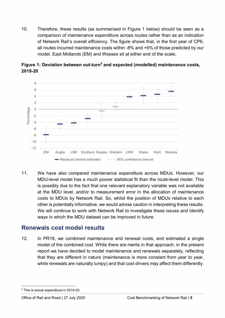
10. Therefore, these results (as summarised in Figure 1 below) should be seen as a comparison of maintenance expenditure across routes rather than as an indication of Network Rail’s overall efficiency. The figure shows that, in the first year of CP6, all routes incurred maintenance costs within -8% and +6% of those predicted by our model. East Midlands (EM) and Wessex sit at either end of the scale.
Figure 1: Deviation between out-turn5 and expected (modelled) maintenance costs, 2019-20
-12
-10
-8
-6
-4
-2
0
2
4
6
8
EM Anglia LNE Scotland Sussex Western LNW Wales Kent Wessex
Perc
enta
ge
Residual (central estimate) 95% confidence interval
11. We have also compared maintenance expenditure across MDUs. However, our MDU-level model has a much poorer statistical fit than the route-level model. This is possibly due to the fact that one relevant explanatory variable was not available at the MDU level, and/or to measurement error in the allocation of maintenance costs to MDUs by Network Rail. So, whilst the position of MDUs relative to each other is potentially informative, we would advise caution in interpreting these results. We will continue to work with Network Rail to investigate these issues and identify ways in which the MDU dataset can be improved in future.
Renewals cost model results 12. In PR18, we combined maintenance and renewal costs, and estimated a single
model of the combined cost. While there are merits in that approach, in the present report we have decided to model maintenance and renewals separately, reflecting that they are different in nature (maintenance is more constant from year to year, while renewals are naturally lumpy) and that cost drivers may affect them differently.
5 This is actual expenditure in 2019-20.
Office of Rail and Road | 27 July 2020 Cost Benchmarking of Network Rail | 6
13. While this change has greatly improved our modelling of maintenance costs, it has also highlighted that our approach to the modelling of renewals needs further work. For instance, our current model is not able to account for the year-on-year fluctuations in renewals as much as we would like. Similarly, we are unable to factor in possible trade-offs between maintenance and renewals activities. That is why, although we present results from our renewals model, our comparisons between Network Rail routes focus on maintenance costs only.
Next steps 14. We are publishing this analysis now, despite some of the shortcomings highlighted
above and the need for further work to interpret these results, because we want to be transparent about progress in our analysis and there is value in sharing emerging results. We will now be working to understand the cost variations highlighted by these results, the issues with the MDU analysis and to improve our future analysis of renewals expenditure. We are keen to receive feedback on this work from Network Rail and from other stakeholders.
15. As we improve our understanding of the underlying causes for unexplained differences in expenditure between business units, and improve our analysis with more data and more effective modelling of MDUs and renewals, we envisage this type of information becoming a more influential element of our reporting toolkit and an input into our efficiency assessment of Network Rail during our next periodic review.

Office of Rail and Road | 27 July 2020 Cost Benchmarking of Network Rail | 7
1. Introduction 1.1 This report presents ORR's latest cost benchmarking analysis of Network Rail,
which compares maintenance and renewals costs across routes (using data covering the financial years 2011-12 to 2019-20), and maintenance costs across maintenance delivery units (MDUs) (using data covering financial years 2014-15 to 2019-20).
1.2 At this stage in the control period, the key objectives of this work are to improve our understanding of Network Rail’s cost drivers and to improve the robustness of our cost benchmarking approach.
1.3 In time, and as our confidence in this evidence base increases, we expect this type of analysis: (1) to become a more influential element of our reporting toolkit; and (2) to input into our efficiency assessment of Network Rail during the next periodic review.
What is cost benchmarking? 1.4 Cost benchmarking involves comparing past expenditure across business units,
after controlling for the effect of observable underlying differences. By ‘controlling for’ we mean that we separate out the effect that differences in observable cost drivers are expected to have on overall expenditure. We do this by identifying statistical patterns in the data using a regression model.
1.5 Cost benchmarking results can be used for a number of purposes. These include to set efficiency targets (typically as part of a periodic review); to identify unexplained cost differences and underlying sources of good or bad practice; to set prices (or access charges in the case of rail infrastructure); or to forecast future costs as the result of changes in outputs.
Limitations 1.6 Any statistical model is only as good as its data. Measurement error (for example,
by wrongly attributing cost incurred in one business unit to another), omitted variables (the absence of important cost drivers from the data), or too small a sample size can all weaken the robustness of results.
1.7 Despite some outstanding issues with omitted variables, we consider that the quality and size of our route maintenance dataset is good enough to compare maintenance costs. But the MDU analysis and data are not as robust. We will continue to identify ways in which the MDU dataset can be improved in future.
1.8 For renewals, there does not appear to be a sufficiently strong and stable relationship over time between renewals expenditure and observable cost drivers at route level. We are beginning to explore alternative data such as expenditure gathered at the level of asset types.
Office of Rail and Road | 27 July 2020 Cost Benchmarking of Network Rail | 8
Background 1.9 Cost benchmarking has been used by ORR to help set efficiency targets for Network
Rail in the 2008 periodic review (PR08) and the 2013 periodic review (PR13). In both PR08 and PR13, we compared Network Rail, as a whole, against a number of European peers. Whilst we used this international comparison to inform our determination, we also recognised that there are limitations in this type of analysis, especially in the absence of high quality and consistent data across countries.
1.10 In PR18, our approach shifted towards comparing Network Rail’s domestic business units, i.e. operating routes and MDUs, building on internal analysis undertaken by Network Rail during PR13. Although we recognise that there remained inherent differences between these business units that could not be controlled for, this analysis provided a useful top-down check on efficiency targets calculated through a more granular, bottom-up, assessment of Network Rail’s business plans.
1.11 We published our PR18 cost benchmarking analysis (here) and committed to update it annually. We also stated our intention to make greater use of comparative regulation in CP6, and we expected cost benchmarking to play a central role in this. The present document is the first of a series of annual cost benchmarking reports to be published during CP6.
Progress since PR18 1.12 This update includes significant improvements compared to our PR18 analysis.
Firstly, we have added four years’ worth of data to the PR18 five-year route dataset and two-year MDU dataset. That equates to an additional 40 data points in the route dataset and an additional 148 data points in the MDU dataset. This has allowed us to include more cost drivers in the model, which translates into more robust estimates and a significant reduction in the size of unexplained variations.
1.13 Secondly, in our route analysis, we now have separate maintenance and renewals models. This reflects that they are different in nature (maintenance is more constant from year to year, while renewals are naturally lumpy) and that cost drivers may affect them differently. By separating the two categories of expenditure, we obtain more robust and more understandable results from the maintenance model, with much lower unexplained differences in maintenance costs between routes. On the other hand, the current model structure cannot take account of the potential interaction between maintenance and renewals activities. This is something we will seek to address in our next annual publication.
Reporting our results 1.14 In the past, we have presented cost benchmarking results as efficiency scores,
which show how far each business unit is from a best-performing benchmark. This benchmark is typically a theoretical construct that combines the best features of the best performing business units.

Office of Rail and Road | 27 July 2020 Cost Benchmarking of Network Rail | 9
1.15 In the present analysis, we compare out-turn expenditure at the business unit level against expected expenditure based on our statistical model. Results are presented as deviations from expected cost. These represent cost variations between business units that cannot be explained statistically by observable characteristics and therefore require further investigation. We highlight the largest outliers in the latest available year (both in terms of costs higher and lower than expected), as there is probably more to learn by focusing our attention on those business units.
1.16 We are continuously working to improve our cost benchmarking evidence base and hope to make significant progress on the modelling of MDUs and renewals over the coming year. However, we are choosing to publish this work now, alongside the Annual Efficiency and Finance Assessment (available here) to ensure we are transparent about our progress to date, the evolution in our thinking since PR18, and to seek feedback from Network Rail and other stakeholders on our approach and results.
1.17 As we improve our understanding of the underlying causes for unexplained differences in expenditure between business units, and improve our analysis with more and better data and more effective modelling of MDUs and renewals, we envisage this type of information becoming a more central element of our reporting toolkit. Our analysis can be used in part as a reputational tool to help drive improved performance within Network Rail, and in part as an indication of where ORR should focus its detailed analysis, monitoring and engagement.
Report structure 1.18 Chapter 2 describes our analysis and the results for maintenance and renewals
costs across Network Rail’s routes. Chapter 3 covers maintenance costs at MDU level and includes a consistency check between route and MDU-level results.

Office of Rail and Road | 27 July 2020 Cost Benchmarking of Network Rail | 10
2. Route-level analysis Introduction 2.1 Regions are geographical business units responsible for operations, maintenance
and renewals activities, functioning with a degree of devolved accountability from Network Rail’s central management structure. Regions are further divided into routes and Network Rail can allocate the majority of maintenance expenditure to the route level.
2.2 The number of routes and their boundaries has evolved over time. During control period 4 (CP4), Network Rail moved to a ten-route structure6. During control period 5 (CP5), London North Eastern was merged with East Midlands, and Kent was merged with Sussex, resulting in eight geographical routes. At the beginning of control period 6 (CP6), Network Rail again reviewed its organisational structure, resulting in the creation of five geographical regions (Scotland, North West & Central, Eastern, Southern, and Wales & Western). Network Rail still has routes, although there are now 14 of them7. The routes are now a sub-geography of the five regions.
2.3 Despite these organisational changes, Network Rail has continued to be able to allocate financial and operational information at the level of its original ten-route structure, and provides that information to ORR8. The benchmarking approach we use requires as much consistently recorded information over a period of time as possible. We therefore use the ten routes as the basis of our analysis as that is the longest times series we have. Annex C shows how those ten routes map onto Network Rail’s current structure.
2.4 In this chapter, we describe the models we have estimated to explain maintenance and renewals expenditure at route level, as a function of key cost drivers. We then compare routes based on the proportion of maintenance expenditure that our model is unable to explain based on available data.
2.5 One important difference between the present work and our PR18 analysis is that we now compare maintenance and renewals costs separately. This has greatly improved our modelling of maintenance costs, but has highlighted shortcomings in
6 Anglia, East Midlands, Kent, LNE, LNW, Scotland, Sussex, Wales, Wessex, and Western. 7 Anglia, East Coast, North & East, East Midlands, West Coast Mainline South, North West, Central, Kent, Sussex,
Network Rail High Speed, Scotland, Wales, Wessex and Western. 8 There is a risk that the recent re-structuring, and ORR’s subsequent decision to regulate Network Rail at region rather
than route level, could lead to the loss of more granular information consistent with historical data. We plan to continue to require Network Rail to provide information for cost benchmarking purposes at a sufficiently granular level that is consistent over time. At the same time, we will be considering over the coming year how to adapt our analysis and the way that its results are communicated to best align with Network Rail’s current structure.

Office of Rail and Road | 27 July 2020 Cost Benchmarking of Network Rail | 11
our analysis of renewals. Our comparison of routes therefore focuses exclusively on maintenance.
2.6 Our analysis shows a statistically significant relationship between a route’s maintenance expenditure, the amount of traffic it carries, the length of track maintained, the complexity of its network and its asset performance.
2.7 In terms of cost performance, our analysis shows that, in the first year of CP6, all routes incurred maintenance costs within -8% and +6% of those predicted by our model. East Midlands and Wessex sit at either end of the scale.
2.8 This chapter is organised as follows: the next section (Routes context) compares the ten routes in terms of their respective expenditure, asset characteristics and network usage, providing context for our results. The following section (Analysis) describes the data and methodology, and presents the model results. In the final section we use this information to compare cost performance across routes.
Routes context 2.9 This section provides a comparison of routes’ average expenditure, traffic density,
some network characteristics and local wages by way of context. All monetary variables are in 2019-20 prices9.
2.10 Total expenditure: Figure 2 shows a breakdown of Network Rail’s total 2019-20 expenditure (excluding financing costs), which amounted to c. £8.9bn. Combined maintenance and renewals costs – the subject of this analysis – accounted for over 50% of Network Rail’s total expenditure (excluding financing costs).
Figure 2: Breakdown of expenditure categories (exc. financing costs), 2019-20
2,908
2,477
1,824
1,737
33%
28%
20%
19%
0 500 1,000 1,500 2,000 2,500 3,000 3,500
Renewals
Operations
Enhancements
Maintenance
£m
9 All expenditure variables in this report were sourced from the Network Rail’s Regulatory Financial Statements. All other network characteristic variables were collected from Network Rail’s Annual Returns or directly supplied by Network Rail.

Office of Rail and Road | 27 July 2020 Cost Benchmarking of Network Rail | 12
2.11 Maintenance and renewals expenditure: Figure 3 below shows average maintenance and renewals spend per track-km by route between 2011-12 and 2019-20. On average, across all years and routes, Network Rail spent £151k per track-km. Sussex was the highest spender (£230k per track-km) whilst Scotland and Wales spent the least (£110k and £104k per track-km, respectively).
Figure 3: Breakdown of average total maintenance and renewals expenditure per track-km, 2011-12 to 2019-20
168136
114 113 107 97 91 78 81 76
62
5958 51
41 5037
34 29 28
151
0
25
50
75
100
125
150
175
200
225
250
Sussex Kent Anglia Wessex Western LNW LNE EM Scotland Wales
£k p
er tr
ack-
km
Renewals Maintenance GB average
2.12 Proportion of track renewed: Figure 4 below shows the volume of track renewed as a proportion of total route track-km. The variation in this variable is likely to be one of the explanations for the variation in total maintenance and renewals expenditure across routes.
Figure 4: Proportion of track renewed, 2011-12 to 2019-20
6.96.3 6.0 5.5 5.3 5.1 5.0 4.8 4.3 3.9
5.3
0
1
2
3
4
5
6
7
8
Sussex Wessex EM LNE Scotland Western Kent Anglia Wales LNW
Perc
enta
ge
GB average

Office of Rail and Road | 27 July 2020 Cost Benchmarking of Network Rail | 13
2.13 In Figure 4, we observe that, on average, Network Rail renewed 5.3% of its track each year between 2011-12 and 2019-20. The Sussex route renewed its track at the highest rate (6.9%), whilst LNW renewed at the lowest rate (3.9%).
2.14 Network utilisation: network utilisation is a key metric that measures the amount of traffic using the network. Figure 5 below compares traffic density (total train-km per track-km) for the nine-year period. On average, traffic density on the GB network is 19,350 train-km per track-km. Anglia, Kent, Sussex, Wessex and LNW have a density above the GB average.
Figure 5: Average traffic density (train-km per track-km), 2011-12 to 2019-20
31,3
56
23,4
20
23,0
21
22,2
86
19,9
63
17,1
17
16,4
62
15,2
84
13,7
41
10,8
54
19,350
0
5,000
10,000
15,000
20,000
25,000
30,000
35,000
Sussex Wessex Anglia Kent LNW LNE Western EM Scotland Wales
Trai
n-km
per
trac
k-km
GB average
2.15 Sussex has the highest traffic density by some margin (62% above the national average) followed by Wessex (21% above national average). This may partly explain why its maintenance and renewals expenditure per track-km is higher than the other routes. On the other hand, Scotland and Wales10 have the lowest traffic density – a possible explanation for their low maintenance and renewals expenditure per track-km. As an example of the differences, traffic density in Sussex was almost three times as much as in Wales over 2011-12 to 2019-20.
2.16 Average track used life11: Figure 6 below shows that Sussex has track with the highest average used life at 63%, possibly being one of the reasons explaining its relatively high maintenance and renewals costs per track-km. However, the data does not seem to point to a consistent relationship between average track used life, and maintenance and renewal expenditure across all routes. For instance, in Scotland and Wales, where maintenance and renewals costs per track-km are lowest, average rail used life is higher than average.
10 Wales has 44% less traffic than the GB average. 11 This is a measure of track assets sustainability. The calculation of the average service life for plain line track is based
on the annual tonnage that has passed over it through its lifetime and the characteristics that affect the rate of its wear and fatigue. The used service life is accumulated year on year from the asset’s installation, dependent on the traffic running over it. A lower percentage represents better sustainability.

Office of Rail and Road | 27 July 2020 Cost Benchmarking of Network Rail | 14
Figure 6: Average track used life, 2011-12 to 2019-20
63 6155 55 55 52 49 46 45 45
53
0
10
20
30
40
50
60
70
Sussex Scotland Wales Kent LNE Anglia Wessex EM Western LNW
Perc
etna
ge
GB average
2.17 In addition to Sussex, Scotland also has a similarly high track asset used life at 61%. On the other hand, East Midlands (EM), Western and LNW routes have the lowest average track used life, c. 45%.
2.18 Proportion of electrified track: Figure 7 below compares the proportion of a route’s track that is electrified (electrified track-km as a proportion of total route track-km)12. As of 2019-20, around half the GB network is electrified, similar to the average across the nine-year period of 48%. There is a high degree of variation in the proportion of electrified track between routes, which is something we take account of in our statistical model.
Figure 7: Proportion of electrified track, 2011-12 to 2019-20
95 92
7165
49
39 39
189
1
48
0
10
20
30
40
50
60
70
80
90
100
Kent Sussex Wessex Anglia LNW LNE Scotland EM Western Wales
Perc
enta
ge
GB average
12 DC third rail and AC overhead line are expected to require very different levels of maintenance. We tested this in PR18
but the results did not conform to our prior expectation. Our latest dataset does not split out AC and DC track-kms. We are working to address this and will look to incorporate this information in future updates.

Office of Rail and Road | 27 July 2020 Cost Benchmarking of Network Rail | 15
2.19 Electrification in Kent and Sussex exceeds 90% of their respective track length. This potentially helps explain their relatively high maintenance and renewals cost per track-km. Likewise, less than 1% of the Wales route is electrified and it has a comparatively low maintenance and renewal cost per track-km. East Midlands and Western have a low proportion of electrified track at 18% and 9%, respectively.
Analysis Data 2.20 The analysis is based on data for financial years 2011-12 to 2019-20, recorded at
the level of the ten routes that were introduced by Network Rail in CP4.
2.21 In 2019-20, there was an accounting change, with a proportion of maintenance costs allocated centrally rather than to routes. We take this into account in our model by separating out the common change in maintenance expenditure across routes between 2018-19 and 2019-20 that cannot be attributed to observable cost drivers.
Dependent variable 2.22 In previous analyses (PR08, PR13 and PR18), our preferred dependent variable
was the sum of maintenance and renewal expenditure. The merits of this approach include the fact that it better captures potential interdependency between maintenance and renewals activities. For example, renewing an asset in one year may reduce maintenance requirements in immediately subsequent years.
2.23 In practice, these two activities are different in nature and may be driven by different factors. Maintenance activities at the route level are less variable over time than renewals, which tend to be undertaken less often and as larger one-off projects to renew specific assets or specific parts of the network.
2.24 Therefore, in the present analysis, we estimate separate models for maintenance and renewals. By separating the two categories of expenditure, we obtain more robust and understandable results.
2.25 While this change has greatly improved our modelling of maintenance costs, it has also highlighted that our approach to the modelling of renewals needs further improvement. For instance, our current model is not able to account for year-on-year fluctuations in renewals as fully as we would like. Similarly, our model is not yet able to account for possible trade-offs between maintenance and renewals activities. That is why, although we also present some results for our renewals model, our comparisons between Network Rail’s routes focus exclusively on maintenance costs.
2.26 We are exploring other approaches that could help address these shortcomings. This could include among others analysing individual projects’ cost data or renewal costs by asset type.

Office of Rail and Road | 27 July 2020 Cost Benchmarking of Network Rail | 16
Independent variables 2.27 In any econometric analysis, a decision has to be made regarding the appropriate
explanatory variables to include in a model, i.e. the business unit characteristics that have the greatest influence on expenditure. Including too many or too few explanatory variables may reduce its ability to produce high quality estimates. We chose our explanatory variables based on the existing literature, on the availability of data, on the performance of different model specifications and on input from asset management experts.
2.28 Although we tested more explanatory variables13, the following table summarises those retained in the final models, alongside the expected direction of the relationship to maintenance and renewals costs and the reasoning behind this.
Table 1: Independent variables used in the route-level model14
Variable Expected
direction for relationship
Reason for relationship
Track-km* (length of track, where 1km of double-tracked route counts as 2 track-km)
Positive A larger network requires more maintenance and renewals which implies higher expenditure.
Passenger traffic density (passenger train-km/track-km) Positive More traffic on the network would likely cause greater
wear and tear.
Freight traffic density (freight train-km/track-km) Positive More traffic on the network would likely cause greater
wear and tear.
Average number of tracks* (avtrack) i.e. track-km divided by route-km
Negative
On a network with multiple tracks, maintenance teams may not need to travel as far on average. Time windows for maintenance activities may be wider on multiple track sections of the network. In addition, there may be less volume of work involved when maintaining 1km of double-track route than 2km of single-track route (for example, due to the volume of ballast and drainage assets).
Switches and crossings density i.e. number of switches and crossings divided by track-km Positive
The number of switches and crossings per track-km is an indication of how complex the network is. All else constant, a route with more switches and crossings per track-km incurs more cost to maintain and renew.
13 The cost drivers we tested but decided not to include in our final model include: track average used life, poor and good track geometry, number of breaks and immediate action defects per 100km, number of delay minutes per 1,000 train-km, route-km, and enhancement expenditure. Network Rail and ORR asset management experts have also identified ease of access as a potentially important cost driver. This information was not available at the time of this analysis but we will seek to include it in future updates. This could be proxied for example by duration of possessions.
14 An asterisk next to the variable name indicates that the variable was included in our PR18 analysis.

Office of Rail and Road | 27 July 2020 Cost Benchmarking of Network Rail | 17
Number of service affecting point failures15
Ambiguous
The relationship between cost and quality/performance measures is complex. While a route may be required to spend more in order to maintain a high asset quality/standard (i.e. to keep the number of point failures very low), a route with a high quality network may decide not to undertake maintenance and renewal work (at least in the short term) which means less spending. On the other hand, poor asset performance (i.e. the existence of many point failures) may also require higher spending to raise the quality of the assets. Therefore, the coefficient on this variable should be interpreted carefully.
Proportion of electrified track i.e. amount of electrified track as a percentage of the total track-km
Positive Power supply infrastructure requires additional maintenance and renewals expenditure.
Wage levels (£/week)16
Positive
All else constant, we expect maintenance and renewals cost to be higher in regions with higher wage levels. In practice, this effect may be significantly reduced by the use of national terms and conditions.
Year and Year squared
N/A
The purpose of these terms is to separate out the common trend in expenditure across routes that cannot be attributed to observable cost drivers. It is expected to improve our confidence in the estimated effect of observable cost drivers. The squared term tells us whether the rate of change is uniform or changing over time. The coefficient on year can be interpreted as an annual growth rate.
Year-specific dummy variables (applies to 2019/20)
N/A
The purpose of these terms is to separate out the common change in expenditure across routes due to year-specific exogenous factors that cannot be attributed to observable cost drivers. It is expected to improve our confidence in the estimated effect of observable cost drivers. The coefficient can be interpreted as a deviation from the average annual growth rate given by the coefficient on the Year variable. We use a dummy for year 2019-20 to reflect a change in cost allocation methodology and the step change in maintenance budgets as the result of PR18.
15 This is a measure of asset condition reliability and performance. It is defined as the number of point failures causing train delays on Network Rail's infrastructure. A lower number of service affecting point failures indicates better performance.
16 ONS seasonally adjusted median average weekly earnings (AWE) per local authority. These have been adjusted for inflation and represent real median earnings. As specific Network Rail wages data was not available to us, we used this as a proxy. The data only reflects the level of wages (in general) in each MDU’s geographical area of operation rather than the actual wages paid by Network Rail. We mapped local authorities to Network Rail’s maintenance and delivery units and then aggregated this at route level. We are also aware that there is a degree of harmonisation of terms and conditions across Network Rail, which may attenuate the effect of regional differences in wages.

Office of Rail and Road | 27 July 2020 Cost Benchmarking of Network Rail | 18
Descriptive statistics 2.29 Table 2 below presents some summary statistics that describe the variables in our
models.
Table 2: Summary of variables
Variable Mean Std. Dev. Min Max
Maintenance expenditure (£m) 133 80 52 405
Renewals expenditure (£m) 243 133 52 736
Track-km (km) 3,110 1,694 1,124 6,720
Passenger traffic density (train-km/track-km) 18,145 5,906 9,365 32,113
Freight traffic density (train-km/track-km) 1,205 581 171 2,258
Electrified proportion 0.48 0.32 0.00 0.96
S&C density (number/track-km) 0.6 0.1 0.3 0.9
Service affecting point failures (count) 408 272 118 1,395
Wage levels (£/week) 592 37 516 684
Average number of tracks (track-km/route-km) 2.0 0.2 1.6 2.7
Model specification 2.30 We have adopted the same functional form as in PR18, namely the Cobb Douglas
log-log formulation (i.e. where the dependent variable and most explanatory variables are entered in natural logarithms). With this functional formulation, most coefficients can be interpreted as constant elasticities, i.e. the percentage change in cost resulting from a 1% change in the relevant cost driver.
2.31 For this updated analysis, we have estimated a number of variants of the following
model17:
𝐿𝐿𝐿𝐿 𝐶𝐶𝐶𝐶𝐶𝐶𝐶𝐶 = 𝛽𝛽0 + 𝛽𝛽1 𝐿𝐿𝐿𝐿 𝑇𝑇𝑇𝑇𝑇𝑇𝑇𝑇𝑘𝑘 𝑘𝑘𝑘𝑘 + 𝛽𝛽2 𝐿𝐿𝐿𝐿 𝑃𝑃𝑇𝑇𝐶𝐶𝐶𝐶𝑃𝑃𝐿𝐿𝑃𝑃𝑃𝑃𝑇𝑇 𝑇𝑇𝑇𝑇𝑇𝑇𝑇𝑇𝑇𝑇𝑇𝑇𝑇𝑇 𝑑𝑑𝑃𝑃𝐿𝐿𝐶𝐶𝑇𝑇𝐶𝐶𝑑𝑑 +𝛽𝛽3 𝐿𝐿𝐿𝐿 𝐹𝐹𝑇𝑇𝑃𝑃𝑇𝑇𝑃𝑃ℎ𝐶𝐶 𝐶𝐶𝑇𝑇𝑇𝑇𝑇𝑇𝑇𝑇𝑇𝑇𝑇𝑇 𝑑𝑑𝑃𝑃𝐿𝐿𝐶𝐶𝑇𝑇𝐶𝐶𝑑𝑑 + 𝛽𝛽4 𝐿𝐿𝐿𝐿 𝑇𝑇𝑎𝑎𝐶𝐶𝑇𝑇𝑇𝑇𝑇𝑇𝑘𝑘 +
𝜷𝜷𝟓𝟓 𝑳𝑳𝑳𝑳 𝑷𝑷𝑷𝑷𝑷𝑷𝑳𝑳𝑷𝑷 𝑭𝑭𝑭𝑭𝑷𝑷𝑭𝑭𝑭𝑭𝑭𝑭𝑭𝑭 + 𝜷𝜷𝟔𝟔 𝑳𝑳𝑳𝑳 𝑺𝑺𝑺𝑺𝑷𝑷𝑷𝑷𝑺𝑺𝑺𝑺𝑭𝑭𝑺𝑺 & 𝑪𝑪𝑭𝑭𝑷𝑷𝑺𝑺𝑺𝑺𝑷𝑷𝑳𝑳𝑪𝑪𝑺𝑺 𝑫𝑫𝑭𝑭𝑳𝑳𝑺𝑺𝑷𝑷𝑷𝑷𝑫𝑫 +𝜷𝜷𝟕𝟕 𝑷𝑷𝑭𝑭𝑷𝑷𝑷𝑷𝑷𝑷𝑭𝑭𝑷𝑷𝑷𝑷𝑷𝑷𝑳𝑳 𝑬𝑬𝑭𝑭𝑭𝑭𝑺𝑺𝑷𝑷𝑭𝑭𝑷𝑷𝑬𝑬𝑷𝑷𝑭𝑭𝑬𝑬 𝑻𝑻𝑭𝑭𝑭𝑭𝑺𝑺𝑻𝑻 + 𝛽𝛽8 𝐿𝐿𝐿𝐿𝐿𝐿𝑇𝑇𝑃𝑃𝑃𝑃 +
𝛽𝛽9𝐷𝐷𝐷𝐷𝑘𝑘𝑘𝑘𝑑𝑑 𝑇𝑇𝐶𝐶𝑇𝑇 2019-20 + 𝛽𝛽10 𝑌𝑌𝑃𝑃𝑇𝑇𝑇𝑇 + 𝛽𝛽11 𝑌𝑌𝑃𝑃𝑇𝑇𝑇𝑇2 + 𝑅𝑅𝑇𝑇𝐿𝐿𝑑𝑑𝐶𝐶𝑘𝑘 𝑃𝑃𝑇𝑇𝑇𝑇𝐶𝐶𝑇𝑇
2.32 In PR18, we estimated different variants of the following model18:
17 A bold font means the variable was not controlled for in PR18. 18 A red font means the variable was dropped from the PR18 model.

Office of Rail and Road | 27 July 2020 Cost Benchmarking of Network Rail | 19
𝐿𝐿𝐿𝐿 𝐶𝐶𝐶𝐶𝐶𝐶𝐶𝐶 = 𝛽𝛽0 + 𝛽𝛽1 𝐿𝐿𝐿𝐿 𝑇𝑇𝑇𝑇𝑇𝑇𝑇𝑇𝑘𝑘 𝑘𝑘𝑘𝑘 + 𝛽𝛽2 𝐿𝐿𝐿𝐿 𝑇𝑇𝑇𝑇𝑇𝑇𝑇𝑇𝑇𝑇𝑇𝑇𝑇𝑇 𝐷𝐷𝑃𝑃𝐿𝐿𝐶𝐶𝑇𝑇𝐶𝐶𝑑𝑑 +𝛽𝛽3 𝐿𝐿𝐿𝐿 𝑇𝑇𝑎𝑎𝐶𝐶𝑇𝑇𝑇𝑇𝑇𝑇𝑘𝑘 + 𝛽𝛽4 𝐷𝐷𝐷𝐷𝑘𝑘𝑘𝑘𝑑𝑑 𝑇𝑇𝐶𝐶𝑇𝑇 𝑇𝑇𝑇𝑇𝐿𝐿𝑇𝑇𝑓𝑓 𝑑𝑑𝑃𝑃𝑇𝑇𝑇𝑇 𝐶𝐶𝑇𝑇 𝐶𝐶𝑃𝑃4 + 𝛽𝛽5 𝑌𝑌𝑃𝑃𝑇𝑇𝑇𝑇 +
𝑅𝑅𝑇𝑇𝐿𝐿𝑑𝑑𝐶𝐶𝑘𝑘 𝑃𝑃𝑇𝑇𝑇𝑇𝐶𝐶𝑇𝑇
2.33 Relative to PR18, the latest model controls for asset performance (through the point failures variable), and asset complexity (through S&C density and proportion of electrification). We are now also able to separate the effect of passenger and freight traffic.
Estimation approach 2.34 We tested panel methods, stochastic frontier methods and pooled ordinary least
squares (OLS)19. As in PR18, we settled on a pooled OLS approach. This approach has the advantage of being simple to implement and its results easy to understand.
2.35 With OLS, we estimate a line that passes through the centre of the observed data points. This means that, given the information available, the OLS line defines the average cost that a business unit should incur given the cost drivers we control for in our model. The distance between the OLS line and observed/outturn points is the residual.
2.36 We use these residuals to describe routes’ performance relative to the average of the peer group, after controlling for differences in relevant cost drivers. Figure 8 below illustrates the following: observations above the line, which show that the route in question spent more than expected20, while those observations below the line, show routes that spent less than expected.
Figure 8: Theoretical OLS regression line and cost performance
0
2
4
6
8
10
12
0 1 2 3 4 5 6 7 8 9
Cos
t
Cost Drivers
Below Average Cost
Above Average Cost Expected (average) cost curve
19 For a detailed description of these models and their assumptions, see our PR18 report available here. 20This means the modelled average cost, i.e. how much we would expect a route to have spent given the characteristics
we control for.

Office of Rail and Road | 27 July 2020 Cost Benchmarking of Network Rail | 20
Results 2.37 This section presents and analyses the results of our OLS model estimates.
Table 3: OLS estimated results for maintenance and renewals models
Variable Maintenance model coefficient
Renewals model coefficient
Track-km 0.77*** 0.77***
Passenger traffic density 0.51*** 0.31
Freight traffic density 0.13*** 0.00
Electrified proportion 0.11 -0.1
S&C density 0.21** 0.75***
Service affecting point failures 0.15** 0.15
Wage levels 0.32 0.86
Average number of tracks 0.1 -0.45
Year (average annual unexplained growth rate in maintenance expenditure) 0.09*** 0.12**
Year-squared (change in the annual growth rate over time) 0.00 -0.01*
Dummy for 2019-20 (deviation from the annual growth rate above) -0.11* -0.38***
Constant21 -10.48*** -9.64**
Number of observations 90 90
R2 0.96 0.86
* Statistically significant at the 90% confidence level ** Statistically significant at the 95% confidence level
*** Statistically significant at the 99% confidence level22
21 The constant has no meaningful physical interpretation. Its role is to improve the fit between the model and the data. The coefficient is provided here for completeness and to ensure our results can be replicated.
22 Technically, statistical significance (expressed by the number of stars in the table) tells us there is an effect and that this is unlikely due to chance, while the size of coefficients tells us what the scale of the effect is. The higher the number of stars the more confident in the results we are. More precisely, when we say that a coefficient is statistically significant at the X% level, this means that there is a X% probability that the true underlying parameter is different from zero. In other words, we are almost entirely certain that the parameter is different from zero. This assessment is based on the assumption that the parameter follows a normal, or bell-shaped, probability distribution across the population, with its most likely value being the parameter estimated.

Office of Rail and Road | 27 July 2020 Cost Benchmarking of Network Rail | 21
2.38 Table 3 above shows that, for maintenance costs, there is a statistically significant relationship (at the 90% confidence level or above) between the amount that a route spends on maintenance and the size of the network it maintains, the level of utilisation (traffic), the complexity of that network (S&C density) and the level of asset performance (point failures). The model’s R2 is 0.96. R2 is a measure of goodness-of-fit, i.e. the proportion of the variance in maintenance cost that is explained by the independent variables in the model. This means that our model can explain 96% of the variance in maintenance costs across routes and over time.
2.39 We find little evidence that either the average number of tracks or local wages (across the economy in the area served by the route rather than Network Rail’s specific wages) affect the cost of either maintenance or renewals. We know that there is a high degree of uniformity in wages across routes and so the lack of a significant wage effect is unsurprising. We will work with Network Rail to explore the possibility of obtaining historical route-specific average wages data.
2.40 Similarly, our model seems to suggest that electrification is not an important cost driver23. We expected (from discussions with ORR engineers and Network Rail) this effect would be statistically significant. It is possible that factors such as sample size, measurement error and interactions with other variables in the models may be causing the weak statistical relationship. In future, as more data becomes available, these relationships might become clearer.
2.41 The results in Table 3 above show that, all other factors held constant:
(a) increasing track length by 1%, leads to an increase of 0.13%24 in maintenance expenditure. This suggests that there are economies of scale in network size, i.e. costs increase less than proportionally with the length of track;
(b) increasing passenger traffic density by 1%, increases maintenance costs by 0.51%. Also, a 1% increase in freight traffic density, would increase costs by 0.13%. These results show economies of density – costs increase less than proportionally with traffic;
(c) increasing the density of switches and crossings by 1% increases maintenance costs by 0.21%;
(d) increasing the number of service affecting point failures by 1%, leads to a 0.15% increase in maintenance costs.
23 This may be explained by the fact that in our data, the correlation between the proportion of electrification and both
maintenance and renewals costs is small (0.01 and -0.02 respectively). Furthermore, the proportion of track that is electrified is very stable over time for most routes, and as such, this variable may be acting as a proxy for some other unobserved, time-invariant route characteristics.
24 We calculated this as 0.77 - (0.51 + 0.13) = 0.13 as in this model formulation, the coefficient for track-km contains both the scale effect (i.e. impact of changing the length of the network) and the density effect (i.e. impact of changing the level of network utilisation) while holding everything else constant. Therefore, 0.13 is the scale effect.

Office of Rail and Road | 27 July 2020 Cost Benchmarking of Network Rail | 22
2.42 The results also show that there has been an annual average, real terms, increase in maintenance expenditure of 9% per year, which cannot be explained by changes in network size, traffic or other observable factors. On the other hand, after accounting for observable differences between routes, maintenance expenditure in 2019-20 appears to be 11% below this historical trend. One possible explanation is that this is due to a change in the accounting of maintenance costs, with a proportion of these costs managed centrally rather than by routes. In reality, out-turn maintenance expenditure for Network Rail as a whole has actually increased between 2018-19 and 2019-20 in real terms.
2.43 Note that the purpose of the present work is to compare maintenance expenditure across routes in the most recent year, whilst controlling for differences in observable cost drivers, rather than to measure routes against an external efficiency benchmark or to examine performance changes over time. We therefore take no view here on the cause of the trend identified above. ORR’s separate publication, the Annual Efficiency and Finance Assessment, provides a view on Network Rail’s efficiency in the first year of CP6 (2019-20); our PR18 final determination sets out our expectations for Network Rail’s efficiency improvement over CP6.
Benchmarking routes’ maintenance cost performance 2.44 In the past, we presented cost benchmarking results as efficiency scores, which
show how far each business unit is from a notional high performing benchmark.
2.45 In the present analysis, we compare out-turn costs against expected spend as predicted by our model, given each route’s characteristics. We then list routes according to the amount of unexplained variation.
2.46 Whilst this analysis can help identify unexplained differences in expenditure, it only tells us what is in the data and does not explain, on its own, the causes of those differences. It provides an indication of where we could focus our detailed analysis, monitoring and engagement. It is also one of several sources of evidence that can help inform our overall cost assessment.
2.47 Figure 9 below shows, for each route, the proportion of unexplained cost variance in 2019-2025. A negative number means that the route spent less than expected (according to our statistical model) while a positive number means that the route spent more than expected (according to our statistical model).
25 The lines surrounding the central estimate of a given route’s deviation between out-turn and modelled cost indicate a 95% confidence interval. Given the data available and the robustness of our model, there is a 95% probability that this estimated confidence interval contains the true deviation. A tighter interval indicates a more precise estimate. We have similar information for all the years covered by the analysis but we chose to present the most recent year.

Office of Rail and Road | 27 July 2020 Cost Benchmarking of Network Rail | 23
Figure 9: Deviation between out-turn and expected (modelled) maintenance costs, 2019-20
-12
-10
-8
-6
-4
-2
0
2
4
6
8
EM Anglia LNE Scotland Sussex Western LNW Wales Kent Wessex
Perc
enta
ge
Residual (central estimate) 95% confidence interval
2.48 These results show that, in the first year of CP6, all routes incurred maintenance costs within -8% and +6% of those predicted by our model. East Midlands and Wessex sit at either end of the scale. It is possible that the disparity between modelled and out-turn costs in a given year is due to management discretion on the precise timing of specific maintenance activities. We therefore also looked at our model’s results for 2018-19. They show that these routes remain outliers across both years (see Figure B1 in Annex B), which means that this result cannot be easily explained by normal year on year fluctuations in maintenance activities26. We will explore this further with Network Rail.
26 When we average out the unexplained variance across 2018-19 and 2019-20, the out-turn maintenance expenditure
across four routes (Scotland, Sussex, Wales and Western) is within 1% of that predicted by our model (see figure B2 in annex B). For those routes, the unexplained variance within a given year can therefore be attributed almost entirely to normal annual fluctuations in maintenance activities.

Office of Rail and Road | 27 July 2020 Cost Benchmarking of Network Rail | 24
3. MDU-level analysis Introduction 3.1 Maintenance Delivery Units (MDUs) are operating units within Network Rail regions,
responsible for the majority of the day-to-day upkeep of their designated part of the network. They ensure that the infrastructure (ranging from signals and power supplies, to track and structures) is in good working order. MDUs are not responsible for renewals and this chapter therefore only covers maintenance costs.
3.2 In its recent restructuring (see footnote 1) Network Rail reduced the number of MDUs from 37 to 35. However, in order to maintain comparability with past data, and given that Network Rail is still able to allocate costs using its previous MDU structure, we have analysed maintenance costs using the previous 37 MDU structure. This involved some judgement on our part on how to apportion data on explanatory variables between MDUs (affected by the change) for the most recent year, based on historical data27. Annex C maps the 37 MDUs to Network Rail’s CP4 ten route structure used in our route benchmarking analysis.
3.3 On average, MDUs accounted for around 70% of total network maintenance expenditure during the four years covered by this analysis. The remaining 30% is centrally-managed and it covers activities such as structure examination, major items of maintenance plants and other HQ managed activities.
3.4 In this chapter, we describe the models we have estimated to explain maintenance expenditure at the MDU level as a function of key cost drivers. We then compare MDUs based on the proportion of maintenance expenditure that our model is unable to explain based on available data. We then carry out a consistency check between route-level and MDU-level results. The results of this check suggest that we should place greater confidence in the route-level analysis and that MDU results should be interpreted with caution, and only used to inform comparisons across MDUs.
3.5 Our analysis suggests that there is a statistically significant relationship between an MDU’s maintenance expenditure and the amount of traffic on the network it covers, the length of track maintained, wages in the local area, and network complexity (as measured by the density of switches and crossings, level of electrification, and average number of tracks).
3.6 In terms of cost performance, the analysis shows that, in 2019-20, Peterborough, Doncaster and York lead the group of MDUs that spent less than our model would
27 Woking closed in 2017-18 with activities previously undertaken by Woking moved to Clapham and Eastleigh, which then became Wessex Inner and Wessex Outer. The four MDUs of Bristol, Plymouth, Reading and Swindon were restructured into the three new MDUs of Western East, Western Central and Western West. Network Rail was able to apportion recent expenditure to the parts of the network linked to the old MDUs. However, Network Rail was unable to do the same for information on explanatory variables (e.g. traffic, track km, etc.). We therefore generated missing information for old MDUs by interpolation and extrapolation from historical trends.

Office of Rail and Road | 27 July 2020 Cost Benchmarking of Network Rail | 25
predict. On the other hand, Lancashire & Cumbria, Liverpool, Euston, Sandwell & Dudley and Cardiff appear to have spent more than our model would predict. Peterborough and Lancashire & Cumbria are at either extreme of the distribution.
3.7 This chapter is organised as follows: the next section (MDU context) compares the 37 MDUs in terms of their respective expenditure, asset characteristics and network usage, providing context for our results. The following section (Analysis) describes the data and methodology, and presents the model estimation results. The section after that (Benchmarking) shows how we use this information to compare cost performance across MDUs. The final section compares these findings with those from our route analysis.
MDU context 3.8 This section provides a comparison of MDUs’ average expenditure, traffic density,
some network characteristics and local wages by way of context. All monetary variables are in 2019-20 prices.
3.9 Maintenance expenditure: Figure 10 below shows that MDUs spent, on average, c. £36.7k per year, per km of track. Euston spent the most, £83k per track-km, whilst Perth spent the lowest amount, £14k per track-km.
Figure 10: Average maintenance expenditure per track-km, 2014-15 to 2019-20
36.7
0
10
20
30
40
50
60
70
80
90
Eust
onLo
ndon
Brid
geBl
etch
ley
Cro
ydon
Rom
ford
Cla
pham
Sand
wel
l & D
udle
yR
eadi
ngLa
nc&C
umbr
iaSt
affo
rdO
rpin
gton
Wok
ing
Totte
nham
Brig
hton
Ipsw
ich
Man
ches
ter
Ashf
ord
Don
cast
erPe
terb
orou
ghSa
ltley
Leed
sC
ardi
ffBe
dfor
dN
ewca
stle
Gla
sgow
East
leig
hSw
indo
nLi
verp
ool
Mot
herw
ell
Edin
burg
hBr
isto
lD
erby
Shef
field
Plym
outh
York
Shre
wsb
ury
Perth
£k p
er tr
ack-
km
3.10 Traffic Density: Figure 11 below shows that an MDU was responsible, on average, for 21,000 train-km per kilometre of track. Croydon saw the highest traffic levels over the time period analysed, with 40,300 train-km per track-km, whilst Perth had the lowest traffic density, with 8,000 train-km per track-km.

Office of Rail and Road | 27 July 2020 Cost Benchmarking of Network Rail | 26
Figure 11: Average traffic density (train-km/track-km), 2014-15 to 2019-20
21,097
0
5,000
10,000
15,000
20,000
25,000
30,000
35,000
40,000
45,000Cr
oydo
nEu
ston
Lond
on B
ridge
Read
ing
Clap
ham
Rom
ford
Blet
chle
yPe
terb
orou
ghBr
ight
onBe
dfor
dLe
eds
Totte
nham
Orp
ingt
onSa
ltley
Staf
ford
Wok
ing
Sand
well &
Dud
ley
Man
ches
ter
Edin
burg
hLi
verp
ool
Donc
aste
rIp
swich
Gla
sgow
Ashf
ord
Swin
don
East
leig
hYo
rkBr
istol
Mot
herw
ell
Derb
yCa
rdiff
Newc
astle
Plym
outh
Lanc
&Cum
bria
Shef
field
Shre
wsb
ury
Perth
Trai
n-km
per
trac
k-km
3.11 Network size (track-km): as shown in Figure 12 below, the Lancashire & Cumbria and Derby MDUs are responsible for the longest sections of network, whilst Euston and London Bridge maintain the shortest sections of the network. The average length of track covered by an MDU over the period 2014-15 to 2019-20 is 840 km.
Figure 12: Average track-km, 2014-15 to 2019-20
844
0
200
400
600
800
1,000
1,200
1,400
1,600
1,800
Lanc
&Cum
bria
Der
byYo
rkLi
verp
ool
Perth
Mot
herw
ell
Car
diff
Shre
wsb
ury
Edin
burg
hN
ewca
stle
Saltl
eyBr
isto
lM
anch
este
rEa
stle
igh
Totte
nham
Shef
field
Plym
outh
Swin
don
Pete
rbor
ough
Ipsw
ich
Ashf
ord
Gla
sgow
Wok
ing
Brig
hton
Bedf
ord
Leed
sD
onca
ster
Staf
ford
Rom
ford
Orp
ingt
onC
laph
amBl
etch
ley
Sand
wel
l & D
udle
yR
eadi
ngC
royd
onLo
ndon
Brid
geEu
ston
Trac
k-km

Office of Rail and Road | 27 July 2020 Cost Benchmarking of Network Rail | 27
3.12 Wages: Figure 13 below compares average local wages across the local authority areas covered by each MDU28.
Figure 13: Median weekly wages in an MDU’s local authority, 2014-15 to 2019-20
588
0
100
200
300
400
500
600
700
800
900
Lond
on B
ridge
Eust
onW
okin
gD
erby
Cla
pham
Rea
ding
Cro
ydon
Blet
chle
yEd
inbu
rgh
Rom
ford
Totte
nham
Orp
ingt
onSw
indo
nM
anch
este
rG
lasg
owBr
isto
lSa
ltley
East
leig
hLe
eds
Bedf
ord
Live
rpoo
lC
ardi
ffN
ewca
stle
Mot
herw
ell
Ashf
ord
Brig
hton
Plym
outh
York
Staf
ford
Ipsw
ich
Shef
field
Lanc
&Cum
bria
Perth
Pete
rbor
ough
Don
cast
erSh
rew
sbur
ySa
ndw
ell &
Dud
ley
Wag
e (£
)
3.13 The data suggests that wages in the London Bridge, Euston and Woking MDU areas are highest. On the other hand, the Doncaster, Shrewsbury and Sandwell & Dudley MDU areas have the lowest wages. We note that local wage variations do not necessarily reflect differences in pay across Network Rail routes due to use of national terms and conditions. However, data on average wages by route is not currently available.
3.14 Average number of tracks (track-km/route-km): on average, MDUs have 2.2 tracks. Euston, Peterborough and Reading have the highest number of average tracks at 3.2. Perth has the lowest average number of tracks at 1.3.
3.15 Average electrification across all MDUs was 51% between 2014-15 and 2019-20. Derby, Perth, Plymouth, Sheffield and Shrewsbury were 0% electrified, whilst more than 95% of the track in the Clapham, Croydon, Euston, London Bridge, Orpington and Peterborough MDUs was electrified.
3.16 The network can be classified as primary, secondary and rural. Peterborough has the highest density of primary network at 94%, Eastleigh has the highest density of secondary network at 73% and Glasgow the highest density of rural network at 43%.
28 Data is sourced from the Office for National statistics (ONS) on weekly earnings by local authority. We matched these
local authorities with each of the 37 MDUs geographical area of operation. Note that this weekly wages data is not Network Rail specific. It simply reflects the level of wages in each geographical area covered by MDUs.
Office of Rail and Road | 27 July 2020 Cost Benchmarking of Network Rail | 28
3.17 The network can also be classified into five criticality bands29. The MDUs with the highest density of track within a criticality band are: Bletchley and Euston (84%) for band 1; Bedford (41%) for band 2; Woking (63%) for band 3; Perth (53%) for band 4; and Shrewsbury (51%) for band 5.
Analysis Data 3.18 The analysis is based on data for Network Rail’s 37 MDUs for financial years
2014-15 to 2019-20.
Dependent variable 3.19 The dependent variable is maintenance expenditure allocated to the MDU level,
collected from statement 8c in Network Rail’s Regulatory Financial Statements. This excludes centrally-managed expenditure (structures examination, major items of maintenance plant and other HQ managed activities), amounting to c. 30% of total maintenance expenditure.
Independent variables 3.20 When conducting econometric cost analysis, a decision has to be made on which
business unit characteristics have the greatest influence on expenditure. In PR18, our decision was heavily influenced by the existing literature and availability of data. In this updated analysis, we have scrutinised the candidate variables further, combining theory and previous research with expertise from ORR asset management specialists and from Network Rail.
29 Network Rail defines route criticality as a “measure of the consequence of the infrastructure failing to perform its intended
function, based on the historic cost of train delay per incident caused by the track asset”. Using this measure, each strategic route section (SRS) of the network has been assigned a route criticality band from 1 to 5. The lower the number of the criticality band, the more a delay is likely to cost should infrastructure fail. The classification of each SRS into criticality bands is used in the development of Network Rail’s asset policy as a first step to matching the timing and type of asset interventions.

Office of Rail and Road | 27 July 2020 Cost Benchmarking of Network Rail | 29
3.21 Although we tested many more explanatory variables30, the following table summarises those retained in the final model, alongside the expected direction of the relationship to maintenance costs and the reasons for this.
Table 4: Independent variables used in the MDU-level model31
Variable Expected direction of relationship
Reason for relationship
Track-km (length of track, where 1 km of double-tracked route counts as 2 track-km)
Positive A larger network requires more maintenance, implying higher expenditure.
Proportion of electrified track*32 (electrified track-km/total track-km) Positive Power supply infrastructure requires additional
maintenance to other parts of the asset base.
Switches and crossings density (number of S&C/track-km)33 Positive An MDU with more switches and crossings
per track-requires more maintenance.
Wage levels (£/week)*34
Positive
If we assume that maintenance work in each MDU is carried out largely by the local labour force, then it will cost more in areas where labour costs are higher. In practice, this effect may be significantly reduced by the use of national terms and conditions.
Average number of tracks* (track-km/ route-km)
Negative
On a network with multiple tracks, maintenance teams may not need to travel as far on average. Time windows for maintenance activities may be wider on multiple track sections of the network. In addition, there may be less volume of work involved when maintaining a km of double track route than 2 km of single track route (for example, due to the volume of ballast and drainage assets).
30 The variables tested but dropped from the final model include: number of stations; weather (rainfall, average temperature); proportion of the network in each speed band (i.e. up to 35 mph, 40-75 mph, 80-105 mph and 110-125 mph); electrification proportion divided into overhead line and third rail; proportion of network divided into the primary, secondary and rural network; and combined passenger and train density, etc.
31 An asterisk next to the variable name indicates that the variable was included in our PR18 analysis. 32 DC third rail and AC overhead line are expected to require very different levels of maintenance. We tested this in PR18
but the results did not conform to our prior expectation. Our latest dataset does not split out AC and DC track-km. We are working to address this and will look to incorporate this information in future updates.
33 We retained this over the absolute number of switches and crossings, which is highly correlated with the average number of tracks and track-km.
34 ONS seasonally adjusted median average weekly earnings (AWE) per local authority. These have been adjusted for inflation and represent real median earnings. As specific Network Rail wages data was not available to us, we used this as a proxy. The data only reflects the level of wages (in general) in each MDU’s geographical area of operation rather than the actual wages paid by Network Rail. We are also aware that there is a degree of harmonisation of terms and conditions across Network Rail, which may attenuate the effect of regional differences in wages.

Office of Rail and Road | 27 July 2020 Cost Benchmarking of Network Rail | 30
Criticality 1 and 2 track density35
Positive
More critical sections of the network are likely to require more frequent maintenance (as set out in technical standards) and may need to be kept in a better general condition than other parts of the network. It is also possible that the access time window is narrower on more critical parts of the network, although this effect may also be covered via the traffic density variable.
Passenger train-km* Positive More traffic will likely cause greater wear and tear.
Freight train-km* Positive More traffic will likely cause greater wear and tear.
Year
N/A
The purpose of this term is to separate out the common trend in expenditure across MDUs that cannot be attributed to observable cost drivers. It is expected to improve our confidence in the estimated effect of observable cost drivers. The coefficient on year can be interpreted as an annual growth rate.
Descriptive statistics 3.22 Table 5 below presents summary statistics for the variables in our model.
Table 5: Summary of variables
Variable Mean Std. Dev. Min Max
Maintenance expenditure (£m) 27.0 9.2 15.2 76.3
Track-km (km) 844.1 313.0 352.5 1615.8
Passenger train-km (million train-km) 14.4 3.7 7.5 23.6
Freight train-km (million train-km) 1.2 0.7 0.1 3.7
Electrified proportion 0.5 0.4 0.0 1.0
S&C density (number/km) 0.6 0.2 0.3 1.4
Wage levels (£/week) 588.1 63.1 493.0 771.0
Average number of tracks (route-km/track-km) 2.1 0.5 1.3 3.3
Criticality 1 & 2 proportion 0.3 0.3 0.0 1.0
35 See definition in footnote 29 (section 3.17) above. We have been told by asset management experts that there is currently an on-going process aimed at reclassifying track sections into different criticality bands and that this is most likely to have a material impact on the definition of track criticality bands 1 and 2. They have suggested that, rather than controlling for each band separately, a combined variable would better represent criticality.

Office of Rail and Road | 27 July 2020 Cost Benchmarking of Network Rail | 31
Model specification 3.23 We have adopted the same functional form as in the route cost benchmarking
chapter above, i.e. the Cobb Douglas log-log formulation (i.e. where dependent variable and most explanatory variables are entered in natural logarithms)36. As mentioned above, this functional formulation allows most coefficients to be interpreted as constant elasticities, i.e. the percentage change in cost resulting from a 1% change in the relevant cost driver.
3.24 The latest specification is as follows37:
𝐿𝐿𝐿𝐿 𝑀𝑀𝑇𝑇𝑇𝑇𝐿𝐿𝐶𝐶𝑃𝑃𝐿𝐿𝑇𝑇𝐿𝐿𝑇𝑇𝑃𝑃 𝑇𝑇𝐶𝐶𝐶𝐶𝑇𝑇𝑓𝑓 𝐶𝐶𝐶𝐶𝐶𝐶𝐶𝐶= 𝛽𝛽0 + 𝛽𝛽1 𝐿𝐿𝐿𝐿 𝑇𝑇𝑇𝑇𝑇𝑇𝑇𝑇𝑘𝑘_ 𝑘𝑘𝑘𝑘 + 𝛽𝛽2 𝐿𝐿𝐿𝐿 𝑃𝑃𝑇𝑇𝐶𝐶𝐶𝐶𝑃𝑃𝐿𝐿𝑃𝑃𝑃𝑃𝑇𝑇 𝑇𝑇𝑇𝑇𝑇𝑇𝑇𝑇𝐿𝐿_𝑘𝑘𝑘𝑘+ 𝛽𝛽3 𝐿𝐿𝐿𝐿 𝐹𝐹𝑇𝑇𝑃𝑃𝑇𝑇𝑃𝑃ℎ𝐶𝐶 𝑇𝑇𝑇𝑇𝑇𝑇𝑇𝑇𝐿𝐿_𝑘𝑘𝑘𝑘 + 𝛽𝛽4 𝐸𝐸𝑓𝑓𝑃𝑃𝑇𝑇𝐶𝐶𝑇𝑇𝑇𝑇𝑇𝑇𝑇𝑇𝑃𝑃𝑑𝑑 𝑃𝑃𝑇𝑇𝐶𝐶𝑃𝑃𝐶𝐶𝑇𝑇𝐶𝐶𝑇𝑇𝐶𝐶𝐿𝐿+ 𝜷𝜷𝟓𝟓 𝑳𝑳𝑳𝑳 𝑺𝑺&𝑪𝑪 𝑫𝑫𝑭𝑭𝑳𝑳𝑺𝑺𝑷𝑷𝑷𝑷𝑫𝑫 + 𝛽𝛽6 𝐿𝐿𝐿𝐿 𝐿𝐿𝑇𝑇𝑃𝑃𝑃𝑃 (𝑘𝑘𝑃𝑃𝑑𝑑𝑇𝑇𝑇𝑇𝐿𝐿)+ 𝛽𝛽7 𝐿𝐿𝐿𝐿 𝐴𝐴𝑎𝑎𝑃𝑃𝑇𝑇𝑇𝑇𝑃𝑃𝑃𝑃 𝑇𝑇𝑇𝑇𝑇𝑇𝑇𝑇𝑘𝑘𝐶𝐶+ 𝜷𝜷𝟖𝟖 𝑷𝑷𝑭𝑭𝑷𝑷𝑷𝑷𝑷𝑷𝑭𝑭𝑷𝑷𝑷𝑷𝑷𝑷𝑳𝑳 𝑷𝑷𝑬𝑬 𝑪𝑪𝑭𝑭𝑷𝑷𝑷𝑷𝑷𝑷𝑺𝑺𝑭𝑭𝑭𝑭𝑷𝑷𝑷𝑷𝑫𝑫 𝟏𝟏&𝟐𝟐 + 𝛽𝛽9 𝑌𝑌𝑃𝑃𝑇𝑇𝑇𝑇+ 𝑅𝑅𝑇𝑇𝐿𝐿𝑑𝑑𝐶𝐶𝑘𝑘 𝑃𝑃𝑇𝑇𝑇𝑇𝐶𝐶𝑇𝑇
3.25 In PR18, we estimated different variants of the following model38:
𝐿𝐿𝐿𝐿 𝑀𝑀𝑇𝑇𝑇𝑇𝐿𝐿𝐶𝐶𝑃𝑃𝐿𝐿𝑇𝑇𝐿𝐿𝑇𝑇𝑃𝑃 𝑇𝑇𝐶𝐶𝐶𝐶𝑇𝑇𝑓𝑓 𝐶𝐶𝐶𝐶𝐶𝐶𝐶𝐶 = 𝛽𝛽0 + 𝛽𝛽1 𝐿𝐿𝐿𝐿 𝑇𝑇𝑇𝑇𝑇𝑇𝑇𝑇𝑘𝑘_ 𝑘𝑘𝑘𝑘 + 𝛽𝛽2 𝐿𝐿𝐿𝐿 𝑃𝑃𝑇𝑇𝐶𝐶𝐶𝐶𝑃𝑃𝐿𝐿𝑃𝑃𝑃𝑃𝑇𝑇 𝑇𝑇𝑇𝑇𝑇𝑇𝑇𝑇𝑇𝑇𝑇𝑇𝑇𝑇 𝐷𝐷𝑃𝑃𝐿𝐿𝐶𝐶𝑇𝑇𝐶𝐶𝑑𝑑 + 𝛽𝛽3 𝐿𝐿𝐿𝐿 𝐹𝐹𝑇𝑇𝑃𝑃𝑇𝑇𝑃𝑃ℎ𝐶𝐶 𝑇𝑇𝑇𝑇𝑇𝑇𝑇𝑇𝐿𝐿 𝐷𝐷𝑃𝑃𝐿𝐿𝐶𝐶𝑇𝑇𝐶𝐶𝑑𝑑 +
𝛽𝛽4 𝐸𝐸𝑓𝑓𝑃𝑃𝑇𝑇𝐶𝐶𝑇𝑇𝑇𝑇𝑇𝑇𝑇𝑇𝑃𝑃𝑑𝑑 𝑃𝑃𝑇𝑇𝐶𝐶𝑃𝑃𝐶𝐶𝑇𝑇𝐶𝐶𝑇𝑇𝐶𝐶𝐿𝐿 + 𝛽𝛽5 𝐿𝐿𝐿𝐿 𝑆𝑆𝑃𝑃𝑃𝑃𝑃𝑃𝑑𝑑40−75 𝑑𝑑𝑃𝑃𝐿𝐿𝐶𝐶𝑇𝑇𝐶𝐶𝑑𝑑 +𝛽𝛽6 𝐿𝐿𝐿𝐿 𝐿𝐿𝑇𝑇𝑃𝑃𝑃𝑃(𝑇𝑇𝑎𝑎𝑃𝑃𝑇𝑇𝑇𝑇𝑃𝑃𝑃𝑃) + 𝛽𝛽7 𝐿𝐿𝐿𝐿 𝐴𝐴𝑎𝑎𝑃𝑃𝑇𝑇𝑇𝑇𝑃𝑃𝑃𝑃 𝑇𝑇𝑇𝑇𝑇𝑇𝑇𝑇𝑘𝑘𝐶𝐶 + 𝛽𝛽8 𝑃𝑃𝑇𝑇𝐶𝐶𝑃𝑃𝑇𝑇𝐶𝐶𝑇𝑇𝐶𝐶𝐿𝐿 𝐶𝐶𝑇𝑇 𝐶𝐶𝑇𝑇𝑇𝑇𝐶𝐶𝑇𝑇𝑇𝑇𝑇𝑇𝑓𝑓𝑇𝑇𝐶𝐶𝑑𝑑 1 + 𝑅𝑅𝑇𝑇𝐿𝐿𝑑𝑑𝐶𝐶𝑘𝑘 𝑃𝑃𝑇𝑇𝑇𝑇𝐶𝐶𝑇𝑇
3.26 The latest model controls for network utilisation using passenger and freight traffic rather than the densities associated with the two variables39. The key advantage is a simpler interpretation of the coefficient estimates.
Estimation approach 3.27 We tested panel methods, stochastic frontier methods and pooled ordinary least
squares (OLS). As in PR18, we settled on pooled OLS. This approach has the advantage of being simple to implement and its results easier to understand.
36 By adopting the same approach as in our route level analysis, we were able to compare the two sets of findings which
ultimately increases our understanding of Network Rail’s costs. 37 A bold font indicates new variables relative to PR18. 38 A red colour font indicates variables that were used in PR18 but have not been included in the new model. 39 While the two models are technically equivalent, the coefficient of the network length variable in a model specified with
traffic densities contains both the scale and density measures, which complicates the interpretation. Note that in the route benchmarking analysis, we use traffic densities (train-km/track-km) instead in order to address the high correlation between train-km and other variables.
Office of Rail and Road | 27 July 2020 Cost Benchmarking of Network Rail | 32
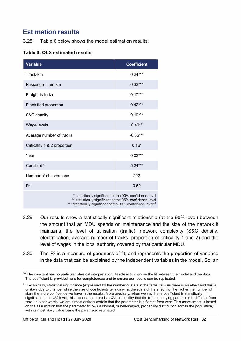
Estimation results 3.28 Table 6 below shows the model estimation results.
Table 6: OLS estimated results
Variable Coefficient
Track-km 0.24***
Passenger train-km 0.33***
Freight train-km 0.17***
Electrified proportion 0.42***
S&C density 0.19***
Wage levels 0.40**
Average number of tracks -0.56***
Criticality 1 & 2 proportion 0.16*
Year 0.02***
Constant40 5.24***
Number of observations 222
R2 0.50
* statistically significant at the 90% confidence level ** statistically significant at the 95% confidence level
*** statistically significant at the 99% confidence level41
3.29 Our results show a statistically significant relationship (at the 90% level) between the amount that an MDU spends on maintenance and the size of the network it maintains, the level of utilisation (traffic), network complexity (S&C density, electrification, average number of tracks, proportion of criticality 1 and 2) and the level of wages in the local authority covered by that particular MDU.
3.30 The R2 is a measure of goodness-of-fit, and represents the proportion of variance in the data that can be explained by the independent variables in the model. So, an
40 The constant has no particular physical interpretation. Its role is to improve the fit between the model and the data. The coefficient is provided here for completeness and to ensure our results can be replicated.
41 Technically, statistical significance (expressed by the number of stars in the table) tells us there is an effect and this is unlikely due to chance, while the size of coefficients tells us what the scale of the effect is. The higher the number of stars the more confidence we have in the results. More precisely, when we say that a coefficient is statistically significant at the X% level, this means that there is a X% probability that the true underlying parameter is different from zero. In other words, we are almost entirely certain that the parameter is different from zero. This assessment is based on the assumption that the parameter follows a Normal, or bell-shaped, probability distribution across the population, with its most likely value being the parameter estimated.

Office of Rail and Road | 27 July 2020 Cost Benchmarking of Network Rail | 33
R2 of 0.50 means that our model can only explain 50% of the variance in maintenance costs, which can be a result of our small sample size, the potential omission of important cost drivers or measurement error.
3.31 The results in Table 6 above show that, all other factors held constant:
a) increasing track length by 1%, whilst keeping traffic constant, would increase maintenance costs by 0.24%. This suggests that there are economies of scale, i.e. costs increase less than proportionally with the length of track;
b) an increase in passenger train-kms of 1%, would increase maintenance costs by 0.33%. The same increase in freight traffic would increase costs by around half (0.17%)42. These results show economies of density – costs increase less than proportionally with traffic;
c) increasing the density of electrified track by 1% would increase maintenance costs by 0.42%. This means that, for instance, going from an average MDU with a network that is 50% electrified to an otherwise similar MDU, which is fully electrified, would be expected to result in 34% higher maintenance costs43;
d) increasing the density of switches and crossings by 1% increases maintenance costs by 0.19%;
e) a 1% difference in local wages would be expected to lead to a 0.40% difference in maintenance costs;
f) it is cheaper to maintain a network with multiple tracks than single tracks. For example, maintaining a given length of track in a single-track route, would be expected to cost 32% more to maintain, than the same length of track in a double track-route44; and
g) increasing the proportion of criticality band 1 and 2 network by 1% would increase maintenance costs by 0.16%.
Benchmarking MDUs’ maintenance cost performance 3.32 Here we compare outturn maintenance costs against expected spend as predicted
by our model, given each MDU’s characteristics. We then list the MDUs according to the amount of the unexplained variation.
3.33 Figure 14 below shows, for each MDU, the proportion of the unexplained cost variance in 2019-2045. A negative number means that the MDU spent less than
42 Freight traffic is heavier but slower than passenger traffic. This means weight and speed may work in different directions
which may make it difficult to make a prediction on the relative sizes of their coefficients. However, if we consider that in our data, freight traffic is very small as compared to passenger traffic, these coefficients are as expected. This is because the small amount of freight traffic means that the average cost for freight is higher than the cost for passenger traffic, implying that for a similar marginal cost increase, the elasticity (i.e. coefficient) of freight must be smaller than the one on passenger traffic. Note: Marginal Cost = Elasticity * Average Cost.
43 This is calculated as 10.42
0.50.42�
44 One km of double-tracked route counts as two track-km. The 32% figure is calculated as 1−0.56
0.5−0.56�
45 We have similar information for all the years covered by the analysis but we chose to present the most recent year.
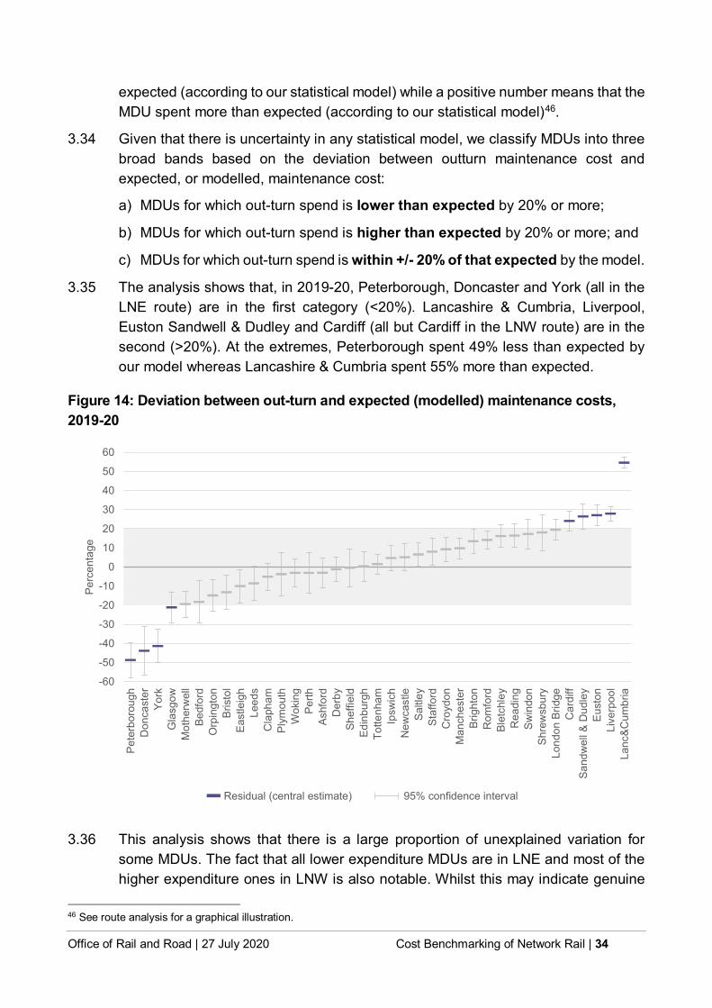
Office of Rail and Road | 27 July 2020 Cost Benchmarking of Network Rail | 34
expected (according to our statistical model) while a positive number means that the MDU spent more than expected (according to our statistical model)46.
3.34 Given that there is uncertainty in any statistical model, we classify MDUs into three broad bands based on the deviation between outturn maintenance cost and expected, or modelled, maintenance cost:
a) MDUs for which out-turn spend is lower than expected by 20% or more;
b) MDUs for which out-turn spend is higher than expected by 20% or more; and
c) MDUs for which out-turn spend is within +/- 20% of that expected by the model.
3.35 The analysis shows that, in 2019-20, Peterborough, Doncaster and York (all in the LNE route) are in the first category (<20%). Lancashire & Cumbria, Liverpool, Euston Sandwell & Dudley and Cardiff (all but Cardiff in the LNW route) are in the second (>20%). At the extremes, Peterborough spent 49% less than expected by our model whereas Lancashire & Cumbria spent 55% more than expected.
Figure 14: Deviation between out-turn and expected (modelled) maintenance costs, 2019-20
-60
-50
-40
-30
-20
-10
0
10
20
30
40
50
60
Pete
rbor
ough
Don
cast
erYo
rkG
lasg
owM
othe
rwel
lBe
dfor
dO
rpin
gton
Bris
tol
East
leig
hLe
eds
Cla
pham
Plym
outh
Wok
ing
Perth
Ashf
ord
Der
bySh
effie
ldEd
inbu
rgh
Totte
nham
Ipsw
ich
New
cast
leSa
ltley
Staf
ford
Cro
ydon
Man
ches
ter
Brig
hton
Rom
ford
Blet
chle
yR
eadi
ngSw
indo
nSh
rew
sbur
yLo
ndon
Brid
geC
ardi
ffSa
ndw
ell &
Dud
ley
Eust
onLi
verp
ool
Lanc
&Cum
bria
Perc
enta
ge
Residual (central estimate) 95% confidence interval
3.36 This analysis shows that there is a large proportion of unexplained variation for some MDUs. The fact that all lower expenditure MDUs are in LNE and most of the higher expenditure ones in LNW is also notable. Whilst this may indicate genuine
46 See route analysis for a graphical illustration.

Office of Rail and Road | 27 July 2020 Cost Benchmarking of Network Rail | 35
disparities in performance, it could also be an indication of measurement error or omitted variables. We will continue to work with Network Rail to understand the reasons behind these differences.
Consistency between route and MDU results 3.37 In Figure 15 below, we compare route results (by unexplained cost variation) from
our route analysis and those implied by this MDU analysis. To do this, we map MDUs to routes, and then sum out-turn and expected (modelled) cost from the MDU data/model up to route level47.
Figure 15: Comparison of routes’ and MDU deviations from expected maintenance cost, 2019-20
-20
-15
-10
-5
0
5
10
15
20
25
30
35
EM Anglia LNE Scotland Sussex Western LNW Wales Kent Wessex
Dev
iatio
n (%
)
Route MDU (grouped)
3.38 Figure 15 shows that there is much greater unexplained variation in the MDU-level model, confirming what we already thought from the much lower R2. This tells us that the route-level model is considerably better at explaining maintenance costs. The figure also shows that the two models lead to very different conclusions in terms of unexplained variation. Note that there is a particularly large disparity between route and MDU results for the LNE and LNW routes, which accords with the observations that these routes contain most of the outlier MDUs.
3.39 We have sought to understand the reason for these disparities. One potential explanation is that the two models do not use exactly the same cost drivers, due to limitations in the data that Network Rail collects. Specifically, information on service affecting point failures is only available at route level. On the other hand, information on the proportion of the network in criticality bands 1 and 2 is only available for years
47 Annex C presents MDUs mapped to their routes.

Office of Rail and Road | 27 July 2020 Cost Benchmarking of Network Rail | 36
2014-15 to 2019-20 and has therefore not been included in the route model (which is based on data going back to 2011-12).
3.40 Another issue is that the maintenance expenditure in the MDU dataset only covers about 70% of the expenditure accounted for at route level. This is because the MDU dataset only includes those maintenance activities actually carried out by MDUs rather than all the maintenance activities carried out within the geographical area covered by an MDU. If the proportion of maintenance activities carried out at the route-level varies between MDUs then this would increase the proportion of unexplained variation in the model.
3.41 Comparing the R2 in the two models, it is clear that the model based on the route dataset is able to explain a much larger proportion of the observed variation in costs (0.96 as opposed to 0.5). We conclude that our route analysis provides the most robust comparison between routes. The MDU analysis may provide useful (if less robust) comparisons between MDUs but the results need to be interpreted with caution and need further investigation.
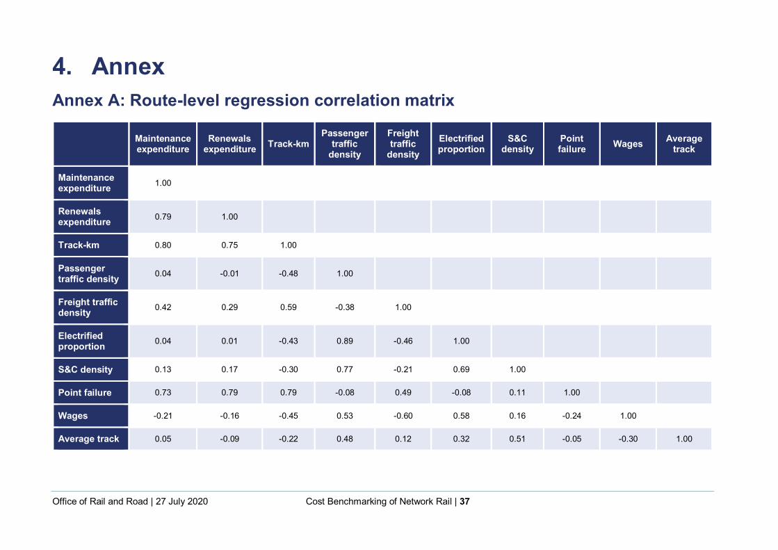
Office of Rail and Road | 27 July 2020 Cost Benchmarking of Network Rail | 37
4. Annex Annex A: Route-level regression correlation matrix
Maintenance expenditure
Renewals expenditure Track-km
Passenger traffic
density
Freight traffic
density Electrified proportion
S&C density
Point failure Wages Average
track
Maintenance expenditure 1.00
Renewals expenditure 0.79 1.00
Track-km 0.80 0.75 1.00
Passenger traffic density 0.04 -0.01 -0.48 1.00
Freight traffic density 0.42 0.29 0.59 -0.38 1.00
Electrified proportion 0.04 0.01 -0.43 0.89 -0.46 1.00
S&C density 0.13 0.17 -0.30 0.77 -0.21 0.69 1.00
Point failure 0.73 0.79 0.79 -0.08 0.49 -0.08 0.11 1.00
Wages -0.21 -0.16 -0.45 0.53 -0.60 0.58 0.16 -0.24 1.00
Average track 0.05 -0.09 -0.22 0.48 0.12 0.32 0.51 -0.05 -0.30 1.00
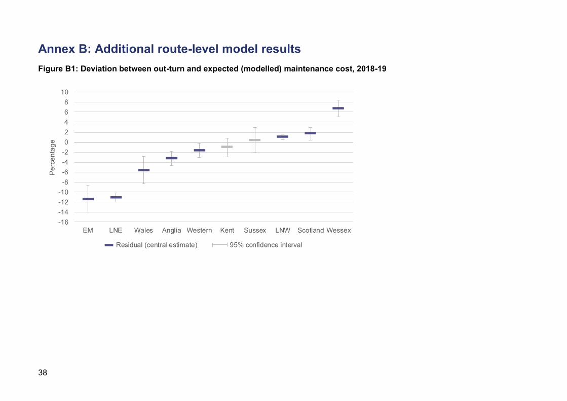
38
Annex B: Additional route-level model results Figure B1: Deviation between out-turn and expected (modelled) maintenance cost, 2018-19
-16-14-12-10
-8-6-4-202468
10
EM LNE Wales Anglia Western Kent Sussex LNW Scotland Wessex
Perc
enta
ge
Residual (central estimate) 95% confidence interval

39
Figure B2: Deviation between out-turn and expected (modelled) maintenance cost, 2018-19 and 2019-20 average
-14-12-10
-8-6-4-202468
10
EM LNE Anglia Wales Scotland Western Sussex Kent LNW Wessex
Perc
enta
ge
Residual (central estimate) 95% confidence interval
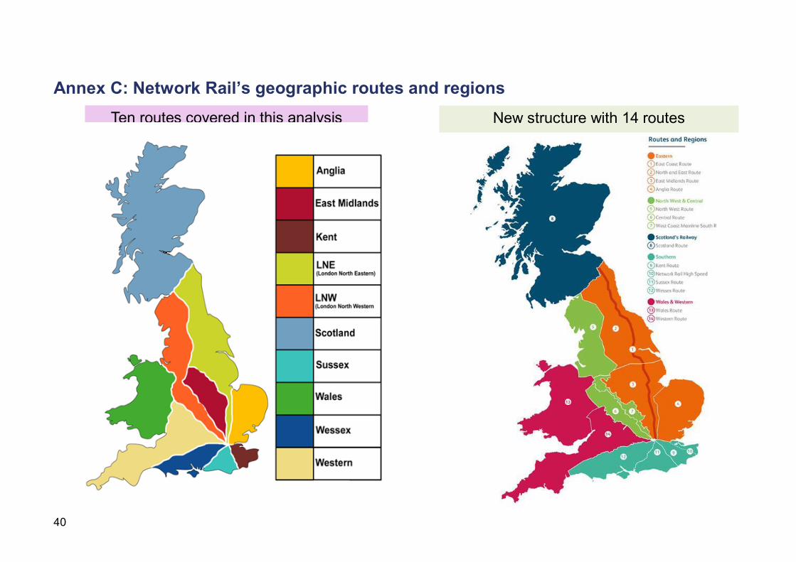
40
Annex C: Network Rail’s geographic routes and regions
Ten routes covered in this analysis New structure with 14 routes

41
Annex D: Mapping of Network Rail’s regions, routes and MDUs
Region CP4 ten routes Maintenance delivery unit (MDU)
Eastern
London North Eastern (LNE) Doncaster, Leeds, Newcastle, Peterborough, Sheffield, York
East Midlands (EM) Bradford, Derby
Anglia Ipswich, Romford, Tottenham
North West & Central London North Western (LNW) Bletchley, Euston, Lancashire & Cumbria, Liverpool, Manchester, Saltley, Sandwell & Dudley, Stafford
Scotland Scotland Edinburgh, Glasgow, Motherwell, Perth
Southern
Wessex Clapham, Eastleigh, Woking
Sussex Brighton, Croydon
Kent Ashford, London Bridge, Orpington
Wales & Western Wales Cardiff, Shrewsbury
Western Bristol, Plymouth, Reading, Swindon

42
© Office of Rail & Road 2020
This publication is licensed under the terms of the Open Government Licence v3.0 except where otherwise stated. To view this licence, visit nationalarchives.gov.uk/doc/open-government-licence/version/3.
Where we have identified any third-party copyright information you will need to obtain permission from the copyright holders concerned.
This publication is available at orr.gov.uk
Any enquiries regarding this publication should be sent to us at orr.gov.uk