cost-effective techniques for continuous …
TRANSCRIPT
University of Nebraska - LincolnDigitalCommons@University of Nebraska - LincolnComputer Science and Engineering: Theses,Dissertations, and Student Research Computer Science and Engineering, Department of
Spring 4-17-2018
COST-EFFECTIVE TECHNIQUES FORCONTINUOUS INTEGRATION TESTINGJingjing LiangUniversity of Nebraska - Lincoln, [email protected]
Follow this and additional works at: https://digitalcommons.unl.edu/computerscidiss
Part of the Computer Engineering Commons, and the Computer Sciences Commons
This Article is brought to you for free and open access by the Computer Science and Engineering, Department of at DigitalCommons@University ofNebraska - Lincoln. It has been accepted for inclusion in Computer Science and Engineering: Theses, Dissertations, and Student Research by anauthorized administrator of DigitalCommons@University of Nebraska - Lincoln.
Liang, Jingjing, "COST-EFFECTIVE TECHNIQUES FOR CONTINUOUS INTEGRATION TESTING" (2018). Computer Scienceand Engineering: Theses, Dissertations, and Student Research. 149.https://digitalcommons.unl.edu/computerscidiss/149
COST-EFFECTIVE TECHNIQUES
FOR CONTINUOUS INTEGRATION TESTING
by
Jingjing Liang
A THESIS
Presented to the Faculty of
The Graduate College at the University of Nebraska
In Partial Fulfilment of Requirements
For the Degree of Master of Science
Major: Computer Science
Under the Supervision of Professors Gregg Rothermel and Sebastian Elbaum
Lincoln, Nebraska
May, 2018
COST-EFFECTIVE TECHNIQUES
FOR CONTINUOUS INTEGRATION TESTING
Jingjing Liang, MS
University of Nebraska, 2018
Adviser: Gregg Rothermel, Sebastian Elbaum
Continuous integration (CI) development environments allow software engineers to
frequently integrate and test their code. While CI environments provide advantages,
they also utilize non-trivial amounts of time and resources. To address this issue,
researchers have adapted techniques for test case prioritization (TCP) and regression
test selection (RTS) to CI environments. In general, RTS techniques select test cases
that are important to execute, and TCP techniques arrange test cases in orders that
allow faults to be detected earlier in testing, providing faster feedback to develop-
ers. In this thesis, we provide new TCP and RTS algorithms that make continuous
integration processes more cost-e↵ective.
To date, current TCP techniques under CI environments have operated on test
suites, and have not achieved substantial improvements. Moreover, they can be in-
appropriate to apply when system build costs are high. In this thesis we explore an
alternative: prioritization of commits. We use a lightweight approach based on test
suite failure and execution history that is highly e�cient; our approach “continu-
ously” prioritizes commits that are waiting for execution in response to the arrival of
each new commit and the completion of each previously commit scheduled for test-
ing. We conduct an empirical study on three datasets, and use the APFD
C
metric
to evaluate this technique. The result shows that, after prioritization, our technique
can e↵ectively detect failing commits earlier.
To date, current RTS techniques under CI environment is based on two windows
in terms of time. But this technique fails to consider the arrival rate of test suites
and only takes the results of test suites execution history into account. In this thesis,
we present a Count-Based RTS technique, which is based on the test suite failures
and execution history by utilizing two window sizes in terms of number of test suites,
and a Transition-Based RTS technique, which adds the test suites’ “pass to mal-
function” transitions for selection prediction in addition to the two window sizes.
We again conduct an empirical study on three datasets, and use the percentage of
malfunctions and percentage of “pass to malfunction” transition metrics to evaluate
these two techniques. The results show that, after selection, Transition-Based tech-
nique detects more malfunctions and more “pass to malfunction” transitions than the
existing techniques.
iv
Contents
Contents iv
List of Figures vii
List of Tables ix
1 Introduction 1
2 Background and Related Work 9
2.1 Related Work . . . . . . . . . . . . . . . . . . . . . . . . . . . . . . . 9
2.2 Continuous Integration . . . . . . . . . . . . . . . . . . . . . . . . . . 12
2.2.1 Continuous Integration at Google . . . . . . . . . . . . . . . . 12
2.2.2 Continuous Integration in Travis CI . . . . . . . . . . . . . . . 13
2.2.3 The Google and Rails Datasets . . . . . . . . . . . . . . . . . 14
2.2.3.1 The Google Dataset . . . . . . . . . . . . . . . . . . 14
2.2.3.2 The Rails Dataset . . . . . . . . . . . . . . . . . . . 15
2.2.3.3 Relevant Data on the Datasets . . . . . . . . . . . . 16
3 Commit Level Prioritization for CI 20
3.1 Motivation . . . . . . . . . . . . . . . . . . . . . . . . . . . . . . . . . 20
3.2 Approach . . . . . . . . . . . . . . . . . . . . . . . . . . . . . . . . . 25
v
3.2.1 Detailed Description of CCBP . . . . . . . . . . . . . . . . . . 26
3.2.2 Example . . . . . . . . . . . . . . . . . . . . . . . . . . . . . . 30
3.3 Empirical Study . . . . . . . . . . . . . . . . . . . . . . . . . . . . . . 31
3.3.1 Objects of Analysis . . . . . . . . . . . . . . . . . . . . . . . . 31
3.3.2 Variables and Measures . . . . . . . . . . . . . . . . . . . . . . 32
3.3.2.1 Independent Variables . . . . . . . . . . . . . . . . . 32
3.3.2.2 Dependent Variables . . . . . . . . . . . . . . . . . . 32
3.3.3 Study Operation . . . . . . . . . . . . . . . . . . . . . . . . . 33
3.3.4 Threats to Validity . . . . . . . . . . . . . . . . . . . . . . . . 34
3.4 Results and Analysis . . . . . . . . . . . . . . . . . . . . . . . . . . . 36
3.4.1 The “Continuous” in CCBP Matters . . . . . . . . . . . . . . 38
3.4.2 Trading Computing Resources and Prioritization . . . . . . . 40
3.4.3 On the Speed of Prioritization . . . . . . . . . . . . . . . . . . 41
3.4.4 On the E↵ect of Wf
Selection . . . . . . . . . . . . . . . . . . 42
3.4.5 Prioritizing Test Suites Within Commits has Limited Impact . 43
3.4.6 Delays in Detecting Failing Commits . . . . . . . . . . . . . . 44
3.5 Summary . . . . . . . . . . . . . . . . . . . . . . . . . . . . . . . . . 45
4 Test Suite Level Selection for CI 46
4.1 Motivation . . . . . . . . . . . . . . . . . . . . . . . . . . . . . . . . . 46
4.2 Approach . . . . . . . . . . . . . . . . . . . . . . . . . . . . . . . . . 52
4.2.1 Count-Based RTS Approach . . . . . . . . . . . . . . . . . . . 52
4.2.2 Transition-Based RTS Approach . . . . . . . . . . . . . . . . . 56
4.3 Empirical Study . . . . . . . . . . . . . . . . . . . . . . . . . . . . . . 61
4.3.1 Objects of Analysis . . . . . . . . . . . . . . . . . . . . . . . . 61
4.3.2 Variables and Measures . . . . . . . . . . . . . . . . . . . . . . 61
vi
4.3.2.1 Independent Variables . . . . . . . . . . . . . . . . . 61
4.3.2.2 Dependent Variables . . . . . . . . . . . . . . . . . . 62
4.3.3 Study Operation . . . . . . . . . . . . . . . . . . . . . . . . . 63
4.3.4 Threats to Validity . . . . . . . . . . . . . . . . . . . . . . . . 64
4.4 Results and Analysis . . . . . . . . . . . . . . . . . . . . . . . . . . . 65
4.4.1 Malfunction Detection E↵ectiveness . . . . . . . . . . . . . . . 67
4.4.2 Pass to Malfunction Transition Detection E↵ectiveness . . . . 73
4.4.3 The E↵ect of We
and W
f
(Werr
/Wfailerr
) Selection . . . . . . . 77
4.5 Summary . . . . . . . . . . . . . . . . . . . . . . . . . . . . . . . . . 81
5 Conclusions and Future Work 82
Bibliography 84
vii
List of Figures
3.1 Intra-commit prioritization on Google post-commit. . . . . . . . . . . . . 21
3.2 Google post-commit arrival queue size over time for five levels of computing
resources . . . . . . . . . . . . . . . . . . . . . . . . . . . . . . . . . . . . 22
3.3 E↵ectiveness of commit prioritization. . . . . . . . . . . . . . . . . . . . 25
3.4 CCBP example. . . . . . . . . . . . . . . . . . . . . . . . . . . . . . . . 30
3.5 APFD
C
on GooglePre . . . . . . . . . . . . . . . . . . . . . . . . . . . . 36
3.6 APFD
C
on GooglePost . . . . . . . . . . . . . . . . . . . . . . . . . . . 37
3.7 APFD
C
on Rails . . . . . . . . . . . . . . . . . . . . . . . . . . . . . . . 37
3.8 APFD
C
on Rails-Compressed . . . . . . . . . . . . . . . . . . . . . . . . 39
3.9 Test suite failures over commits for GooglePost . . . . . . . . . . . . . . 43
4.1 Flow of incoming test suites for Rails over seven days . . . . . . . . . . . 49
4.2 Test suites transitions on Google Pre . . . . . . . . . . . . . . . . . . . . 51
4.3 Failure detection on GooglePost . . . . . . . . . . . . . . . . . . . . . . . 66
4.4 Failure detection on GooglePre . . . . . . . . . . . . . . . . . . . . . . . 66
4.5 Failure detection on Rails . . . . . . . . . . . . . . . . . . . . . . . . . . 66
4.6 Error detection on Rails . . . . . . . . . . . . . . . . . . . . . . . . . . . 66
4.7 FailError detection on Rails . . . . . . . . . . . . . . . . . . . . . . . . . 66
4.8 “Pass to Fail” transition detection on GooglePost . . . . . . . . . . . . . 66
viii
4.9 “Pass to Fail” transition detection on GooglePre . . . . . . . . . . . . . . 67
4.10 “Pass to Fail” transition detection on Rails . . . . . . . . . . . . . . . . . 67
4.11 “Pass to Error” transition detection on Rails . . . . . . . . . . . . . . . . 67
4.12 “Pass to FailError” transition detection on Rails . . . . . . . . . . . . . . 67
4.13 CB technique’s best performance in malfunction detection on Rails (Wf
=
W
err
= W
failerr
= 100) . . . . . . . . . . . . . . . . . . . . . . . . . . . . 71
4.14 TrB technique’s best performance in malfunction detection on Rails (Wf
=
W
err
= W
failerr
= 100) . . . . . . . . . . . . . . . . . . . . . . . . . . . . 71
4.15 “Fail”,“Error” and “FailError” distribution on Rails . . . . . . . . . . . . 71
4.16 CB technique’s best performance in Pass to Malfunction transition detec-
tion on Rails (Wf
= W
err
= W
failerr
= 100) . . . . . . . . . . . . . . . . 76
4.17 TrB technique’s best performance of Pass to Malfunction transition detec-
tion on Rails (Wf
= W
err
= W
failerr
= 100) . . . . . . . . . . . . . . . . 76
4.18 TrB test suite selection on Google Post (Wf
= 100) . . . . . . . . . . . . 78
4.19 TrB test suite selection on Google Post (We
= 1) . . . . . . . . . . . . . 78
ix
List of Tables
2.1 Relevant Data on Objects of Analysis on Commit Level . . . . . . . . . . 17
2.2 Relevant Data on Objects of Analysis on Test Suite Level . . . . . . . . . 17
3.1 Commits, Test Suites, Failures Detected . . . . . . . . . . . . . . . . . . 24
3.2 APFD
C
for Continuous vs. One-Time Prioritization . . . . . . . . . . . 40
3.3 APFD
C
on GooglePost across Computing Resources . . . . . . . . . . . 41
4.1 TB Selection Process . . . . . . . . . . . . . . . . . . . . . . . . . . . . . 48
4.2 CB Selection Process . . . . . . . . . . . . . . . . . . . . . . . . . . . . . 54
4.3 TrB Selection Process . . . . . . . . . . . . . . . . . . . . . . . . . . . . 59
1
Chapter 1
Introduction
Continuous integration (CI) environments automate the process of building and test-
ing software, allowing engineers to merge changed code with the mainline code base at
frequent time intervals. Companies like Google [36], Facebook [17, 44], Microsoft [16],
and Amazon [49] have adopted CI and its ability to better match the speed and scale
of their development e↵orts. The usage of CI has also dramatically increased in
open source projects [25], facilitated in part by the availability of rich CI frameworks
(e.g., [3, 27, 50, 51]).
CI environments do, however, face challenges. System builds in these environ-
ments are stunningly frequent; Amazon engineers have been reported to conduct
136,000 system deployments per day [49], averaging one every 12 seconds [37]. Fre-
quent system builds and testing runs can require non-trivial amounts of time and
resources [7, 18, 25]. For example, it is reported that at Google, “developers must
wait 45 minutes to 9 hours to receive testing results” [36], and this occurs even though
massive parallelism is available. For reasons such as these, researchers have begun to
address issues relevant to the costs of CI, including costs of building systems in the
CI context [7], costs of initializing and reconfiguring test machines [18], and costs of
2
test execution [15, 36, 45, 58].
Regression Testing Challenges in CI. Where testing in CI development environ-
ments is concerned, researchers have investigated strategies for applying regression
testing more cost-e↵ectively. In particular, researchers [6, 15, 28, 34, 35, 36, 58] have
considered techniques (created prior to the advent of CI) that utilize regression test
selection (RTS) (e.g., [10, 19, 24, 32, 38, 39, 41, 46, 55, 56]) and test case prioritiza-
tion (TCP) (e.g., [2, 12, 23, 34, 42, 57]). RTS techniques select test cases that are
important to execute, and TCP techniques arrange test cases in orders that allow
faults to be detected earlier in testing, providing faster feedback to developers.
In CI environments, traditional RTS and TCP techniques can be di�cult to apply.
A key insight behind most traditional techniques is that testing-related tasks such as
gathering code coverage data and performing program analyses can be performed in
the “preliminary period” of testing, before changes to a new version are complete. The
information derived from these tasks can then be used during the “critical period”
of testing after changes are complete and when time is more limited. This insight,
however, applies only when su�ciently long preliminary periods are available, and
this is not typical in CI environments. Instead, in CI environments, test suites arrive
continuously in streams as developers perform commits. Prioritizing individual test
cases is not feasible in such cases due to the volume of information and the amount
of analysis required. For this reason, RTS and TCP techniques for CI environments
have typically avoided the use of program analysis and code instrumentation, and
operated on test suites instead of test cases.
TCP in CI. Prior research focusing on TCP in CI environments [15, 58] has resulted
in techniques that either reorder test suites within a commit (intra-commit) or across
commits (inter-commit). Neither of these approaches, however, have proven to be
3
successful.
Intra-commit prioritization schemes rarely produce meaningful increases in the
rate at which faults are detected. As we shall show in Section 3.1, intra-commit
techniques prioritize over a space of test suites that is too small in number and can
be quickly executed, so reordering them typically cannot produce large reductions in
feedback time. This approach also faces some di�culties. First, test suites within
commits may have dependencies that make reordering them error-prone. Second, test
scripts associated with specific commits often include semantics that adjust which test
suites are executed based on the results of test suites executed earlier in the commit;
these devices reduce testing costs, but may cease to function if the order in which
test suites are executed changes.
Inter-commit techniques have the potential for larger gains, but are founded on
unrealistic assumptions about CI environments. In these environments, developers
use commits to submit code modules, and each commit is associated with multiple test
suites. These test suites are queued up until a clean build of the system is available
for their execution. Extending the execution period of a commit’s test suites over
time (across commits) increases the chance for test suites to execute over di↵erent
computing resources, hence requiring additional system build time. Given the cost of
such builds (Hilton et al. [25] cite a mean cost of 500 seconds per commit, and for the
Rails artifact in our study the mean cost ratio of building over testing was 41.2%),
this may not be practical.
We conjecture that in CI environments, prioritizing test suites (either within or
between commits) is not the best way to proceed. Instead, prioritization should be
performed on commits, a process we refer to as inter-commit prioritization. Inter-
commit prioritization avoids the costs of performing multiple builds, and problems
involving test suite dependencies and the disabling of cost-saving devices for reduc-
4
ing testing within commits. We further believe that inter-commit prioritization will
substantially increase TCP’s ability to detect faulty commits early and provide faster
feedback to developers.
In this work, we investigate this conjecture by providing an algorithm that pri-
oritizes commits. An additional key di↵erence between our TCP approach and prior
work, however, is that we do not wait for a set or “window” of test suites (or in our
case, commits) to be available, and then prioritize across that set. Instead, we pri-
oritize (and re-prioritize) all commits that are waiting for execution “continuously”
as prompted by two events: (1) the arrival of a new commit, and (2) the completion
of a previously scheduled commit. We do this using a lightweight approach based on
test suite failure and execution history that has little e↵ect on the speed of testing.
Finally, our approach can be tuned dynamically (on-the-fly) to respond to changes in
the relation of the incoming testing workload to available testing resources.
RTS in CI. Prior research [15] provided a lightweight RTS technique which used
two windows based on time (we refer this as the TB technique) to track how recently
test suites1 have been executed and revealed failures, to select a subset of test suites
instead of all test suites for execution. It did so in two ways. First, if a test suite T
has failed within a given “failure window” (i.e., within a time W
f
prior to the time
at which T is being considered for execution again) then T should be executed again.
Second, if the first condition does not hold, but test suite T has not been executed
within a given “execution window” (i.e., within a time We
prior to the time at which
T is being considered for execution again) then T should be executed again. The first
condition causes recently failing test suites to be re-executed, and the second causes
1Traditionally, RTS techniques have been applied to test cases. In this work we apply them totest suites, primarily because the datasets we use to study our approach include test suites, andanalysis at the test suite level is more e�cient. The approaches could also, however, be performedat the level of test cases.
5
test suites that have not recently failed, but that have not been executed in quite a
while, to be executed again.
The TB technique utilizes relatively lightweight analysis, and does not require code
instrumentation, rendering it appropriate for use within the continuous integration
process. The empirical study result shows that the TB RTS technique can greatly
improve the cost-e↵ectiveness of testing. While the results were encouraging, the TB
technique also had several limitations.
First, the windows that the TB technique relies on are measured in terms of time,
which means that it does not consider the arrival rate of test suites. In the middle
of a busy work day, test suites can arrive far more frequently than, say, on a Sunday
evening. The TB technique does not account for this, and this can result in selection
of excessively large, or excessively small, numbers of test suites. More importantly,
this can conceivably result in the selection of test suites that are not as cost-e↵ective
as might be desired.
To make up for this limitation, we provide a modified Count-Based RTS technique
(CB), which utilizes two window sizes in terms of numbers of test suites instead of
time. For example, when deciding whether to execute a given test suite T that is
being considered for execution, the technique considers whether T has failed within
the past Wf
test suite executions, or whether T has not been executed at all during
the past We
test executions, and bases its selection on that.
Second, the TB and CB RTS methods are both based on the results (“pass” or
“fail” status) of test suite executions by using a failure window to check whether
the test suite has recently failed. However, these techniques fail to consider the
“transitions” between test suites’ executions, where “transition” means a transition
from one execution status to another. For example, if a test suite T has been executed
3 times, and the corresponding execution statuses are: “pass”, “pass”, and “fail”; then
6
T is considered to have 3 transitions: “new to pass”, “pass to pass”, and“pass to fail”.
Therefore, if T has both “pass” and “fail” statuses, then T has 4 possible transitions:
“pass to pass”, “pass to fail”, “fail to pass”, “fail to fail”. To detect a failure, however,
test suite T can have only two possible transitions: “pass to fail” and “fail to fail”. In
the the result-based techniques (TB and CB), for any test suite, if it has been detected
to fail, it would be selected for execution multiple times in the following arrivals, and
more failures (if existing) could be detected. Obviously, the result-based techniques
could help to detect “fail to fail” transitions. However, result-based techniques fail
to consider the greater importance of “pass to fail” transitions. In addition, “pass
to fail” transitions could provide us with more information than just “pass to pass”,
“fail to pass” or “fail to fail” transitions. Most transitions (more than 99% on the
datasets we study) are “pass to pass” transitions, and such transitions could only tell
us that the testing process is successful. RTS techniques, however, aim to detect more
malfunctions; therefore, we want to select these transitions as little as possible. “Fail
to fail” transitions could indicate that the same problem still exists, or that some
other new problems have occurred. In actual testing, developers will definitely look
for such problems and re-execute the program to check whether these problems are
fixed when a failure occurs, so this type of transition is less important to test. “Fail
to pass” transitions could tell us that a problem has been fixed and there is no need
to select a test suite again for execution. In contrast to all of these, “pass to fail”
transitions signal that a new problem has occurred, and if the test suite repetitively
has “pass to fail” transitions, this could provide us with more information about code
changes, and we could assume that code related to the test is churning.
To make up for this limitation, we provide a Transition-Based RTS technique
(TrB), which keeps track of the percentage of each test suite’s “pass to fail” transitions
in addition to just utilizing two windows. For example, when deciding whether to
7
execute a given test suite T that is being considered for execution, the technique
considers whether T has failed within the pastWf
test suite executions, whether T has
not been executed at all during the pastWe
test executions, or whether T ’s percentage
of “pass to fail” transitions is higher than a threshold and bases its selection on that.
To investigate the e↵ectiveness of the CB and TrB techniques, we use the follow-
ing two metrics for evaluation. First, since the CB RTS technique is based on the
conjecture that some test suites’ execution results are inherently better than others
at revealing failures, we use the percentage of malfunctions detection as a metric to
evaluate the technique, and also apply this metric to the TrB technique for a com-
parison. Second, since the TrB RTS technique is based on the conjecture that test
suites’ “pass to fail” transitions could provide more information about problems in
the code, and detecting “pass to fail” transitions could potentially help us make more
precise malfunction predictions, we use the percentage of “pass to fail” transitions as
a metric to evaluate the performance of the TrB technique and also apply this metric
to the CB technique for comparison.
We conducted empirical studies of our new TCP and RTS approaches on three
non-trivial data sets associated with projects that utilize CI. The results of CCBP
(the new TCP technique) show that our algorithm can be much more e↵ective than
prior TCP approaches. Our results also reveal, however, several factors that influence
our algorithm’s e↵ectiveness, with implications for the application of prioritization in
CI environments in general. The results of the CB and TrB RTS techniques show that
both of these two algorithms could detect the malfunctions and “pass to malfunction”
transitions cost-e↵ectively, and after comparison, the TrB technique has a slightly
better performance under both of the two metrics.
The remainder of this paper is organized as follows. Chapter 2 provides back-
ground information and related work. Chapter 3 presents our commit level priori-
8
tization technique. Chapter 4 presents test suite level RTS techniques. Chapter 5
concludes and discuss future work.
9
Chapter 2
Background and Related Work
We next provide background information on Continuous Integration and on related
work about test case prioritization (TCP) and regression test selection (RTS).
2.1 Related Work
Let P be a program, let P 0 be a modified version of P , and let T be a test suite for P .
Regression testing is concerned with validating P
0. To facilitate this, engineers often
begin by reusing T , but this can be expensive. Thus, a wide variety of approaches
have been developed for rendering reuse more cost-e↵ective via test case prioritization
(TCP) (e.g., [9, 12, 23, 42, 47, 48, 57]) and regression test selection (RTS) (e.g., [19,
32, 38, 39, 41, 46, 55]).
Other Related Work. There has been considerable research on predicting fault-
prone modules in software systems. Some of this work has considered dynamic pre-
diction, as we do, most notably work by Hassan et al. [22] and Kim et al. [30]. This
work, however, does not consider CI environments, or attempt to use fault proneness
information in the service of regression testing techniques.
10
There has been some recent work on techniques for testing programs on large
farms of test servers or in the cloud (e.g., [4, 31, 48]). This work, however, does not
specifically consider CI processes or regression testing.
Hilton et al. [25] report results of a large-scale survey of developers to understand
how and why they use or do not use CI environments. One of the implications
they derive is that CI requires non-trivial time and resources, and thus, the research
community should find ways to improve CI build and testing processes.
Test Case Prioritization. Test case prioritization (TCP) techniques reorder the
test cases in T such that testing objectives can be met more quickly. One potential
objective involves revealing faults, and TCP techniques have been shown to be capable
of revealing faulting more quickly.
Do et al. [8], Walcott et al. [53], Zhang et al. [59], and Alspaugh et al. [1] study test
case prioritization in the presence of time constraints such as those that arise when
faster development-and-test cycles are used. This work, however, does not consider
test history information or CI environments. Other work [2, 29, 54] has used test
history information and information on past failures to prioritize test cases, as do we,
but without considering CI environments.
Prioritization in CI has emerged as a large issue but until this work it focused
exclusively on test cases or suites. Jiang et al. [28] consider CI environments, and
mention that prioritization could be used following code commits to help organiza-
tions reveal failures faster, but their work focuses on the ability to use the failures
thus revealed in statistical fault localization techniques. Busjaeger and Xie [6] present
a prioritization algorithm that uses machine learning to integrate various sources of
information about test cases. They argue that such algorithms are needed in CI
environments, and they analyze the needs for such algorithms in one such environ-
11
ment, but their focus remains on prioritizing individual test cases. Marijan et al. [35]
present prioritization algorithms that also utilize prior test failure information to per-
form prioritization but focus on individual test cases. Yoo et al. [58], also working
with data from Google, describe a search-based approach for using TCP techniques
in CI environments for test suites within commits. Elbaum et al. [15] also describe a
prioritization technique for use in CI environments considering information on past
test failures and elapsed time since prior test executions. Their approach, however,
applies to individual test suites without considering commit boundaries. They also
perform prioritization over windows of test suites and not continuously.
Regression Test Selection. Regression test selection (RTS) techniques select, from
test suite T , a subset T 0 that contains test cases that are important to re-run. When
certain conditions are met, RTS techniques can be safe; i.e., they will not omit test
cases which, if executed on P
0, would reveal faults in P
0 due to code modifications [43].
Memon et al. [36], working in the context of Google’s CI processes, investigate
approaches for avoiding executing test cases that are unlikely to fail, and for helping
developers avoid actions leading to test case failures. Like our work, this work relies
on test selection and attempts to reduce resources in testing; however, the work
only relies on the result of test suite, not considering transitions between test suites.
Gligoric el al. [19] provide a novel approach focusing on improvement of regression
test selection, but this technique is based on file dependencies. Oqvist el al. [38]
consider regression test selection under CI environments, but this work is based on
static analysis.
In prior work Elbaum et al. [15], worked on Google datasets and applied their
improved RTS and TCP techniques by using time windows to track the test suites’
failure history and execution history to the CI development environment. However
12
in this thesis, we change the time windows (window sizes in terms of time) to count
windows (windows sizes in terms of numbers of test suites) and consider “pass to
malfunction” transitions as a factor for selection prediction. As objects of analysis,
we utilize a Rails dataset [33] in addition to the Google datasets [14, 33].
2.2 Continuous Integration
Conceptually, in CI environments, each developer commits code to a version control
repository. The CI server on the integration build machine monitors this repository
to determine whether changes have occurred. On detecting a change, the CI server
retrieves a copy of the changed code from the repository and executes the build
and test processes related to it. When these processes are complete, the CI server
generates a report about the result and informs the developer. The CI server continues
to poll for changes in the repository, and repeats the previous steps.
There are several popular open source CI servers including Travis CI [51], GoCD [20],
Jenkins [27], Buildbot [5], and Integrity [26]. Many software development companies
are also developing their own [16, 36, 44, 49]. In this paper we utilize data gath-
ered from a CI testing e↵ort at Google, and a project managed under Travis CI, and
the next two sections provide an overview of these CI processes. Section 2.2.1, 2.2.2
and 2.2.3 provides a more quantitative description of the data analyzed under these
processes.
2.2.1 Continuous Integration at Google
The Google dataset we rely on in this work was assembled by Elbaum et al. [15] and
used in a study of RTS and TCP techniques; the dataset is publicly available [14].
Elbaum et al. describe the process by which Google had been performing CI, and
13
under which the dataset had been created. We summarize relevant parts of that
process here; for further details see Reference [36].
Google utilizes both pre-commit and post-commit testing phases. When a devel-
oper completes his or her coding activities on a module M , the developer presents
M for pre-commit testing. In this phase, the developer provides a change list that
indicates modules that they believe are directly relevant to building or testing M .
Pre-submit testing requests are queued for processing and the test infrastructure per-
forms them as resources become available, using all test suites relevant to all of the
modules listed in the change list. The commit testing outcome is then communicated
to the developer.
Typically, when pre-commit testing succeeds for M , a developer submits M to
source code control; this causes M to be considered for post-commit testing. At this
point, algorithms are used to determine the modules that are globally relevant to
M , using a coarse but su�ciently fast process. This includes modules on which M
depends as well as modules that depend on M . All of the test suites relevant to these
modules are queued for processing.
2.2.2 Continuous Integration in Travis CI
Travis CI is a platform for building and testing software projects hosted at GitHub.
When Travis CI is connected with a GitHub repository, whenever a new commit
is pushed to that repository, Travis CI is notified by GitHub. Using a specialized
configuration file developers can cause builds to be triggered and test suites to be
executed for every change that is made to the code. When the process is complete,
Travis sends notifications of the results to the developer(s) by email or by posting
14
a message on an IRC channel. In the case of pull requests,1 each pull request is
annotated with the outcome of the build and test e↵orts and a link to the build log.
Rails is a prominent open source project written in Ruby, that relies on continuous
integration in Travis CI. As of this writing, Rails has undergone more than 50,000
builds on Travis CI. Rails consists of eight main components with their own build
scripts and corresponding test suites: Action Mailer (am), Action Pack (ap), Action
View (av), Active Job (aj), Active Model (amo), Active Record (ar), Active Support
(as) and Railties. The eight Rails components are executed for di↵erent rvm imple-
mentations, which includes Ruby MRI v 2.2.1, Ruby-head, Rbx-2, and JRuby-head.
Each pair of components and rvms is executed in a di↵erent job. When a commit is
pushed to a branch, the commit contains multiple jobs, and within a job, there are
multiple test suites for testing.
2.2.3 The Google and Rails Datasets
2.2.3.1 The Google Dataset
The Google Shared Dataset of Test Suite Results (GSDTSR) contains information on
a sample of over 3.5 million test suite executions, gathered over a period of 30 days,
applied to a sample of Google products. The dataset includes information such as
anonymized test suite identifiers, change requests (commits), outcome statuses of test
suite executions, launch times, and times required to execute test suites. The data
pertains to both pre-commit and post-commit testing phases, and we refer to the two
data subsets and phases as “GooglePre” and “GooglePost”, respectively. We used the
first 15 days of data because we found discontinuities in the later days. At Google,
1The fork & pull collaborative development model used in Travis CI allows people to fork anexisting repository and push commits to their own fork. Changes can be merged into the repositoryby the project maintainer. This model reduces friction for new contributors and it allows independentwork without up-front coordination.
15
test suites with extremely large execution times are marked by developers for parallel
execution. When executed in parallel, each process is called a shard. For test suites
that had the same test suite name and launch times but di↵erent shard numbers,
we merged the shards into a single test suite execution. After this adjustment, there
were 2,506,926 test suite execution records. More information about this dataset can
be found in the Google Dataset archive [14] and the clean Google Dataset archive
[33].
2.2.3.2 The Rails Dataset
Rails is a prominent open source project written in Ruby [40]. As the time in which we
harvested its data, Rails had undergone more than 35,000 builds on Travis CI. Rails
consists of eight main components with their own build scripts and test suites. Rails
has a global Travis build script that is executed when a new commit is submitted to
any branch or pull request. (Pull requests are not part of the source code until they
are successfully merged into a branch, but Travis still needs to test them.) For each
commit, the eight Rails components are tested under di↵erent Ruby Version Manager
(rvm) implementations. Each pair of components and rvms is executed in a di↵erent
job.
When collecting data for Rails, we sought to gather a number of test suite ex-
ecutions similar to those found in GSDTSR. Because each Rails’ commit executes
around 1200 test suites on average, we collected 3000 consecutive commits occurring
over a period of five months (from March 2016 to August 2016). From that pool of
commits, we removed 196 that were canceled before the test suites were executed.
We ended up with a sample of 3,588,324 test suite executions, gathered from 2,804
builds of Rails on Travis CI.
To retrieve data from Rails on Travis CI, we wrote two Ruby scripts using methods
16
provided by the Travis CI API [52]: one downloads raw data from Travis CI and the
other transforms the data into a required format. This last step required the parsing
of the test suite execution reports for Rails by reverse engineering their format. The
resulting dataset includes information such as test suite identifiers, test suite execution
time, job and build identifiers, start times, finish times and outcome statuses (fail or
pass). More information about this dataset can be found at https://github.com/
elbaum/CI-Datasets.git.
2.2.3.3 Relevant Data on the Datasets
In the Google datasets, each test suite execution record has a status field that contains
only two types of statuses: “pass” and “fail”. In the Google dataset, a “failing test
suite” is any test suite with a “fail” status. But in the Rails dataset, there is no such
field for each test suite execution record. Instead, each test suite execution record
contains the number of passing test cases, failing test cases, and error test cases.
Thus, there are 4 possible combinations: (1) test suites that contain only passing test
cases; (2) test suites that contain at least 1 failing test case and 0 error test cases
(may contain passing test cases); (3) test suites that contain at least 1 error test case
and 0 failing test cases (may contain passing test cases); (4) test suites that contain
at least 1 failing test case and at least 1 error test case (may contain passing test
cases).
Normally, if a test suite contains at least 1 failing test case and 0 error test cases
(combination 2), this test suite is defined as “fail”. However, each test suite is assigned
a boolean parameter “allow failure”, and if “allow failure” is set to be true, even the
test suite is failing, it does not make the commit fail (a commit is considered to fail
when at least one of its associated test suites fails).
Therefore, for the commit level prioritization technique, we filter the Rails dataset
17
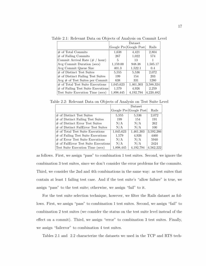
Table 2.1: Relevant Data on Objects of Analysis on Commit LevelDataset
Google Pre Google Post Rails
# of Total Commits 1,638 4,421 2,804# of Failing Commits 267 1,022 574Commit Arrival Rate (# / hour) 5 13 1Avg Commit Duration (secs) 1,159.00 948.38 1,505.17Avg Commit Queue Size 401.3 1,522.1 0.4# of Distinct Test Suites 5,555 5,536 2,072# of Distinct Failing Test Suites 199 154 203Avg # of Test Suites per Commit 638 331 1280# of Total Test Suite Executions 1,045,623 1,461,303 3,588,324# of Failing Test Suite Executions 1,579 4,926 2,259Test Suite Execution Time (secs) 1,898,445 4,192,794 4,220,482
Table 2.2: Relevant Data on Objects of Analysis on Test Suite LevelDataset
Google Pre Google Post Rails
# of Distinct Test Suites 5,555 5,536 2,072# of Distinct Failing Test Suites 199 154 191# of Distinct Error Test Suites N/A N/A 262# of Distinct FailError Test Suites N/A N/A 100# of Total Test Suite Executions 1,045,623 1,461,303 3,592,266# of Failing Test Suite Executions 1,579 4,926 4460# of Error Test Suite Executions N/A N/A 5940# of FailError Test Suite Executions N/A N/A 2424Test Suite Execution Time (secs) 1,898,445 4,192,794 4,562,222
as follows. First, we assign “pass” to combination 1 test suites. Second, we ignore the
combination 3 test suites, since we don’t consider the error problems for the commits.
Third, we consider the 2nd and 4th combinations in the same way: as test suites that
contain at least 1 failing test case. And if the test suite’s “allow failure” is true, we
assign “pass” to the test suite; otherwise, we assign “fail” to it.
For the test suite selection technique, however, we filter the Rails dataset as fol-
lows. First, we assign “pass” to combination 1 test suites. Second, we assign “fail” to
combination 2 test suites (we consider the status on the test suite level instead of the
e↵ect on a commit). Third, we assign “error” to combination 3 test suites. Finally,
we assign “failerror” to combination 4 test suites.
Tables 2.1 and 2.2 characterize the datasets we used in the TCP and RTS tech-
18
nique studies, and help provide context and explain our findings.
Table 2.1 is a summary of the datasets used for our new TCP technique, and
includes information on commits, test suites, and test suite executions. For commits,
we include data on the total number of commits, the total number of failing commits
(a commit is considered to fail when at least one of its associated test suites fails), the
commit arrival rate measured in commits per second, the average commit duration
measured from the time the commit begins to be tested until its testing is completed,
and the average commit queue size computed by accumulating the commit queue size
every time a new commit arrives and dividing it by the total number of commits.
Within the test suite information, we provide the number of distinct test suites that
were executed at least once under a commit, the number of distinct test suites that
failed at least once, and the average number of test suites triggered by a commit.
Regarding test suite executions, we include the total number of test suite executions,
the total number of failing test suite executions, and the total time spent executing
test suites measured in seconds.
Table 2.2 is a summary of the datasets used for our new RTS techniques, which
includes information on test suites, and test suite executions. We provide the number
of distinct test suites that were executed at least once, the number of distinct test
suites that failed (contain at least one failing test case and no error test case ) at least
once, the number of distinct test suites that errored (contain at least one errored test
case and no failing test case) at least once, and the number of distinct test suites
that failerrored (contains at least one errored test case and one failing test case)
at least once. Regarding test suite executions, we include the total number of test
suite executions, the total number of failing test suite executions, the total number
of errored test suite executions, the total number of failerrored test suite executions,
and the total time spent executing test suites measured in seconds. Because Google
19
Pre and Google Post do not have “error” or “failerror” test suites, there are “N/A”
values in the corresponding cells.
20
Chapter 3
Commit Level Prioritization for CI
As we noted in Chapter 1, current techniques for prioritizing test cases in CI envi-
ronments have operated at the level of test suites, and the associated prioritization
techniques are intra-commit test suite prioritization and inter-commit test suite prior-
itization. However, these techniques raises potential problems involving dependency
problems and build costs. Therefore, we consider prioritization at the level of com-
mits instead of test suites. In this chapter, we provide our new algorithm and the
results and analysis of an empirical study of the approach.
3.1 Motivation
There are two key motivations for this work. First, existing prioritization techniques,
that prioritize at the level of test suites yield little improvement in the rate of fault
detection. Second, as commits queue up to be tested, they can be prioritized more
e↵ectively.
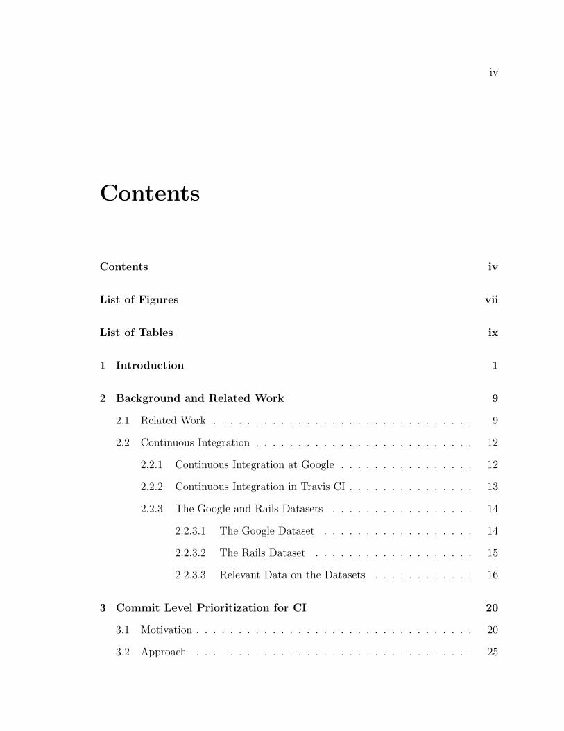
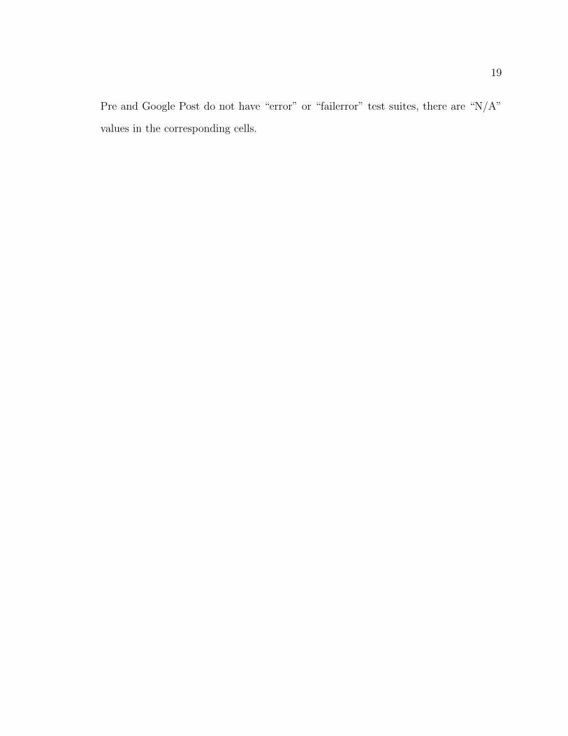
Figure 3.1 plots Google post-commit data supporting the first of these claims.
The horizontal axis represents the passage of time, in terms of the percentage of the
21
0 20 40 60 80 100
020
4060
8010
0
% of Time
% o
f Fai
ling
Test
Sui
tes
Exec
uted
Original APFD = 48.2072%Optimal Intra APFD = 48.2366%
Figure 3.1: Intra-commit prioritization on Google post-commit.
total testing time needed to execute a stream of almost 1.5 million test suites. The
vertical axis denotes the percentage of test suites that have failed thus far relative to
the number of test suites that fail over the entire testing session.
The figure plots two lines. One line, denoted by triangles, represents the “Original”
test suite order. This depicts the rate at which failing test suites are executed over
time, when they (and the commits that contain them) are executed in the original
order in which they arrived for testing in the time-line captured by the Google dataset,
with no attempt made to prioritize them.1 The second line, denoted by diamonds
that are smaller than the triangles, represents an “Optimal Intra-commit” order. In
this order, commits continue to be executed in the order in which they originally
arrived, but within each commit, test suites are placed in an order that causes failing
test suites to all be executed first. (Such an optimal order cannot be achieved by
1The “gaps” between points at around the 58% time are caused by a pair of commits thatcontained large numbers of test suites that failed.
22
0 20 40 60 80 100
050
010
0015
0020
0025
0030
00
% of Time
Que
ue S
ize
●
●
●
●
● ●
●
●
●
●
cp=1cp=2cp=3cp=4cp=8
Figure 3.2: Google post-commit arrival queue size over time for five levels of comput-ing resources
TCP techniques, because such techniques do not know a priori which test suites fail,
but given test suites for which failure information is known it can be produced a
posteriori to illustrate the best case scenario in comparisons such as this.)
In graphs such as that depicted in Figure 3.1, a test suite order that detects faults
faster would be represented by a line with a greater slope than others. In the figure,
however, the two lines are nearly identical. The gains in rate of fault detection that
could be achieved by prioritizing test suites within commits in this case are negligible.
The actual overall rates of fault detection using the APFD
C
metric for assessing such
rates (discussed in Section 4.3.2.2), also shown in the figure, are 48.2072% for the
original order, versus 48.2366% for the optimal order; this too indicates negligible
benefit.
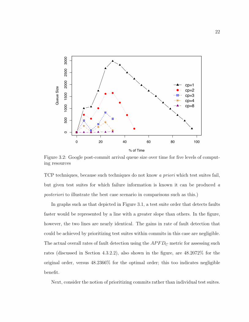
Next, consider the notion of prioritizing commits rather than individual test suites.

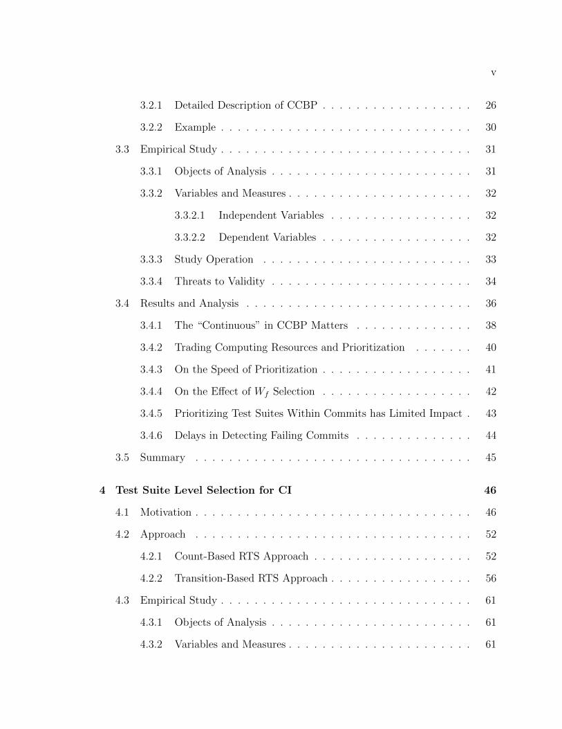
23
Figure 3.2 shows the sizes of several queues of commits over time, for the Google post-
commit dataset, assuming that commits are executed one at a time (not the case at
Google but useful to illustrate trends), and are queued when they arrive if no computer
processors (cp) are available for their execution. Because the execution of test suites
for commits depends on the number of computing resources across which they can be
parallelized, the figure shows the queue sizes that result under five such numbers: 1,
2, 3, 4 and 8. With one computing resource, commits queue up quickly; then they are
gradually processed until all have been handled. As the number of resources increases
up to four, di↵erent peaks and valleys occur. Increasing the number to eight causes
minimal queuing of commits.
What Figure 3.2 shows is that if su�cient resources are not available, commits
do queue up, and this renders the process of prioritizing commits potentially useful.
Clearly, additional computing resources could be added to reduce the queuing of
commits, and for companies like Google and services like Travis, farms of machines
are available. The cost of duplicating resources, however, does become prohibitive
at some point. In the case of Travis, for example, the price for resources increases
by 87% when moving from one to two concurrent jobs. And even for companies like
Google this is an ongoing challenge [36].
The reasons for considering inter-commit prioritization can be illustrated further
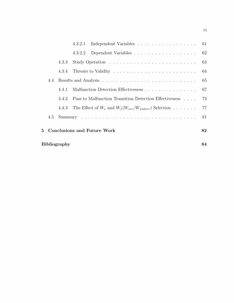
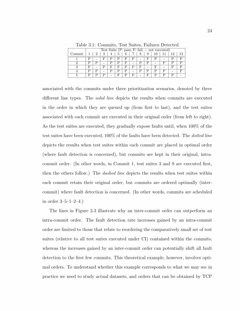
by an example. (We use a theoretical example here for simplicity.) Table 3.1 shows a
set of five commits (Rows 1–5), each containing up to ten test suites (Columns with
headers 1–13), with “F” indicating instances in which test suites fail, “P” indicating
instances in which test suites pass, and “-” indicating instances in which test suites
are not used. Suppose the five commits depicted in Table 3.1 all arrive in a short
period of time and are all queued up for execution, in order from top (“Commit 1”) to
bottom (“Commit 5”). Figure 3.3 plots the fault detection behavior of the test suites
24
Table 3.1: Commits, Test Suites, Failures DetectedTest Suite (P: pass, F: fail, -: not executed)
Commit 1 2 3 4 5 6 7 8 9 10 11 12 13
1 P - F P P P P - F P - P P
2 P P - P P P - P P - P P P
3 F - P F F P P F - F - P P
4 P P - P P P - P P P P - P
5 P P P - F P F - F P P P -
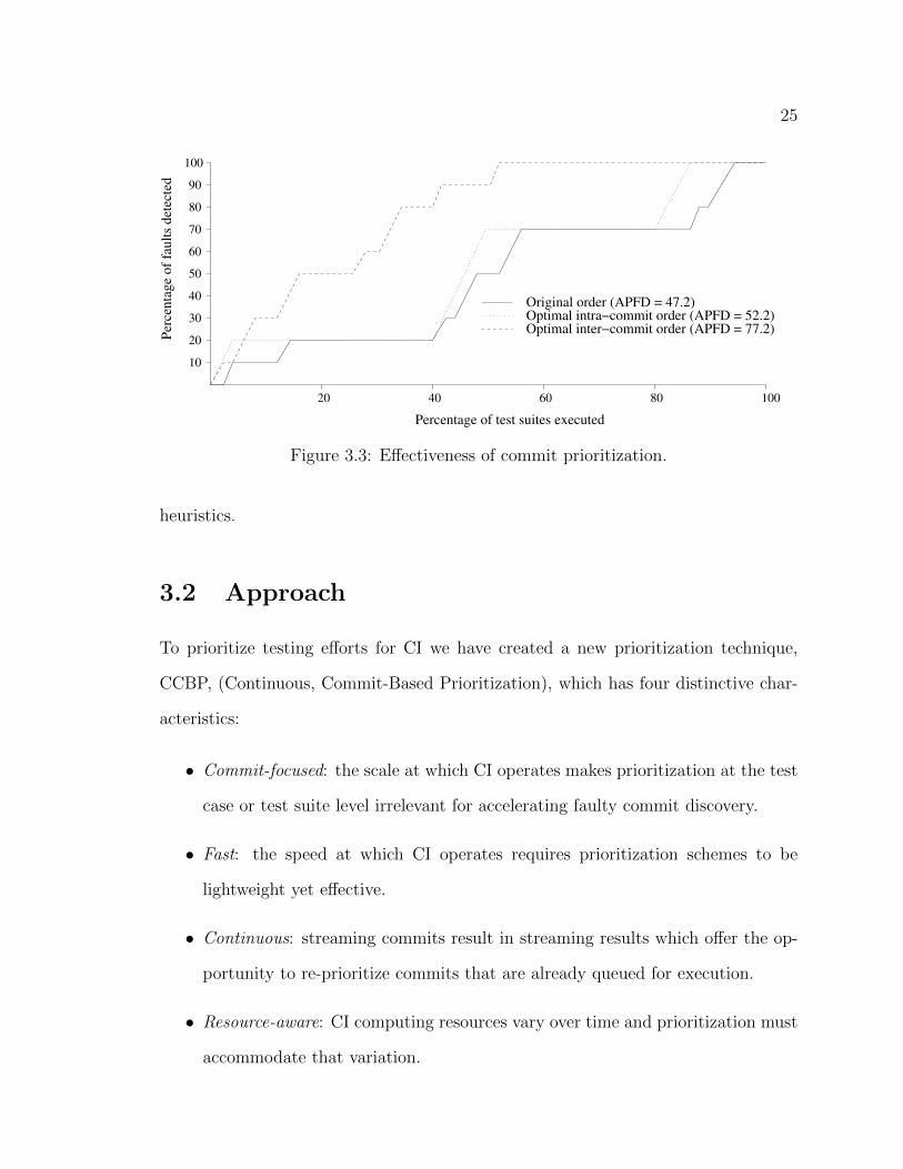
associated with the commits under three prioritization scenarios, denoted by three
di↵erent line types. The solid line depicts the results when commits are executed
in the order in which they are queued up (from first to last), and the test suites
associated with each commit are executed in their original order (from left to right).
As the test suites are executed, they gradually expose faults until, when 100% of the
test suites have been executed, 100% of the faults have been detected. The dotted line
depicts the results when test suites within each commit are placed in optimal order
(where fault detection is concerned), but commits are kept in their original, intra-
commit order. (In other words, in Commit 1, test suites 3 and 9 are executed first,
then the others follow.) The dashed line depicts the results when test suites within
each commit retain their original order, but commits are ordered optimally (inter-
commit) where fault detection is concerned. (In other words, commits are scheduled
in order 3–5–1–2–4.)
The lines in Figure 3.3 illustrate why an inter-commit order can outperform an
intra-commit order. The fault detection rate increases gained by an intra-commit
order are limited to those that relate to reordering the comparatively small set of test
suites (relative to all test suites executed under CI) contained within the commits,
whereas the increases gained by an inter-commit order can potentially shift all fault
detection to the first few commits. This theoretical example, however, involves opti-
mal orders. To understand whether this example corresponds to what we may see in
practice we need to study actual datasets, and orders that can be obtained by TCP
25
Per
centa
ge
of
fault
s det
ecte
d
10
20
30
40
50
60
70
80
90
100
Percentage of test suites executed
20 40 60 10080
Original order (APFD = 47.2)Optimal intra−commit order (APFD = 52.2)Optimal inter−commit order (APFD = 77.2)
Figure 3.3: E↵ectiveness of commit prioritization.
heuristics.
3.2 Approach
To prioritize testing e↵orts for CI we have created a new prioritization technique,
CCBP, (Continuous, Commit-Based Prioritization), which has four distinctive char-
acteristics:
• Commit-focused: the scale at which CI operates makes prioritization at the test
case or test suite level irrelevant for accelerating faulty commit discovery.
• Fast: the speed at which CI operates requires prioritization schemes to be
lightweight yet e↵ective.
• Continuous: streaming commits result in streaming results which o↵er the op-
portunity to re-prioritize commits that are already queued for execution.
• Resource-aware: CI computing resources vary over time and prioritization must
accommodate that variation.
26
CCBP is driven by two events associated with commits: the arrival of a commit for
testing and the completion of the execution of the test suites associated with a commit.
When a commit arrives, it is added to a commit queue and, if computing resources are
available, the queue is prioritized and the highest priority commit begins executing.
When a commit’s processing is complete, a computing resource and new testing-
related information from that commit become available, so any queued commits are
re-prioritized and the highest ranked commit is scheduled for execution.
Note that by this approach, prioritization is likely to occur multiple times on
the same queued commits, as new commits arrive or new information about the
results of a commit become available. For this to be possible, prioritization needs
to be fast enough so that the gains of choosing the right commit are greater than
the time required to execute the prioritization algorithm. As discussed previously,
techniques that require code instrumentation or detailed change analysis do not meet
this criterion when applied continuously, and when used sporadically they tend to
provide data that is no longer relevant. Instead, as in other work [15, 58], we rely
on failure and execution history data to create a prioritization technique that can be
applied continuously.
3.2.1 Detailed Description of CCBP
Algorithm 1 provides a more detailed description of CCBP. The two driving commit
events (commit arrival and commit completion) invoke procedures onCommitArrival
and onCommitTestEnding, respectively. Procedure prioritize performs the actual
prioritization task, and procedure updateCommitInformation performs bookkeeping
related to commits.
CCBP relies on three data structures. The first data structure concerns commits
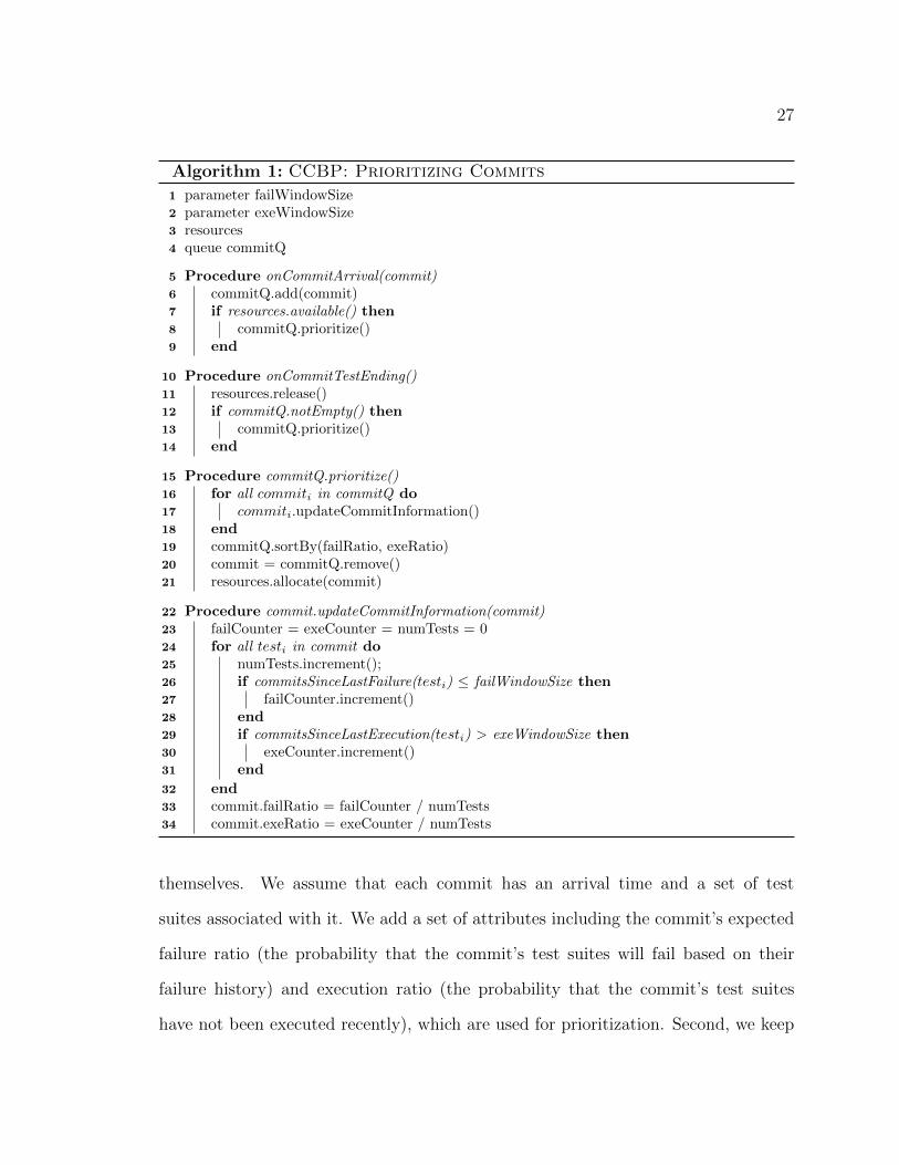
27
Algorithm 1: CCBP: Prioritizing Commits
1 parameter failWindowSize2 parameter exeWindowSize3 resources4 queue commitQ
5 Procedure onCommitArrival(commit)
6 commitQ.add(commit)7 if resources.available() then
8 commitQ.prioritize()9 end
10 Procedure onCommitTestEnding()
11 resources.release()12 if commitQ.notEmpty() then
13 commitQ.prioritize()14 end
15 Procedure commitQ.prioritize()
16 for all commiti in commitQ do
17 commiti.updateCommitInformation()18 end
19 commitQ.sortBy(failRatio, exeRatio)20 commit = commitQ.remove()21 resources.allocate(commit)
22 Procedure commit.updateCommitInformation(commit)
23 failCounter = exeCounter = numTests = 024 for all testi in commit do
25 numTests.increment();26 if commitsSinceLastFailure(testi) failWindowSize then
27 failCounter.increment()28 end
29 if commitsSinceLastExecution(testi) > exeWindowSize then
30 exeCounter.increment()31 end
32 end
33 commit.failRatio = failCounter / numTests34 commit.exeRatio = exeCounter / numTests
themselves. We assume that each commit has an arrival time and a set of test
suites associated with it. We add a set of attributes including the commit’s expected
failure ratio (the probability that the commit’s test suites will fail based on their
failure history) and execution ratio (the probability that the commit’s test suites
have not been executed recently), which are used for prioritization. Second, we keep

28
a single queue of commits that are pending execution (commitQ). Arriving commits
are added to commitQ and commits that are placed in execution are removed from
commitQ, and whenever resources become available commitQ is prioritized. The third
data structure concerns computing resources. In the algorithm, we abstract these so
that when a commit is allocated, the number of resources is reduced, and when a
commit finishes, the resources are released. There are parameters corresponding to the
size of the failure window (failWindowSize) and execution window (exeWindowSize),
measured in terms of numbers of commits, that are important to the prioritization
scheme. In this work we set these parameters to specific constant values, but in
practice they could be adjusted based on changing conditions (e.g., when releasing
a new version for which failures are more likely). We assume there is also a set of
resources available.
Both onCommitArrival (Lines 5–9) and onCommitTestEnding (Lines 10–14), in-
voke prioritize (Lines 15–21). Procedure prioritize updates information about the
commits in the queue (Lines 16-18), and then sorts them (Line 19). This sort func-
tion can be instantiated in many ways. In our implementation, we sort commits in
terms of decreasing order of failRatio values and break ties with exeRatio values, but
other alternatives are possible and we expect this to be an area of active research. The
commit with the highest score is removed from the queue (Line 20) and launched for
execution on the allocated resource (Line 21). Procedure updateCommitInformation
(Lines 22–34) updates a commit’s failRatio and exeRatio. It does this by analyzing
the history of each test suite in the commit. If a test suite has failed within the last
failWindowSize commits, its failure counter is incremented (Lines 26-27). If a test
suite has not been executed within the last exeWindowSize, its execution counter is
incremented (Lines 29-30). These numbers are normalized by the numbers of test
suites in the commits to generate new ratios (Lines 33-34). Intuitively, CCBP favors
29
commits containing a larger percentage of test suites that have failed recently, and in
the absence of failures, it favors commits with test suites that have not been recently
executed.
As presented, for simplicity, CCBP assumes that commits are independent and
need not be executed in specified orders. The empirical studies presented in this paper
also operate under this assumption, as we have discovered no such dependencies
in the systems that we study. Dependencies among commits could, however, be
accommodated by allowing developers to specify them, and then requiring CCBP to
treat dependent commits as singletons in which commit orders cannot be altered. We
leave investigation of such approaches for future work.
Another issue is the potential for a commit to “starve”, as might happen if it has
never been observed to fail and if the pace at which new commits arrive causes the
queue to remain full. This possibility is reduced by the fact that a commit’s execution
counter continues to be incremented, increasing the chance that it will eventually be
scheduled; we return to this issue later in this paper.
For clarity, our presentation of CCBP simplifies some implementation details. For
example, we do not prioritize unless we have multiple items in the commitQ and we
keep a separate data structure for test suites to avoid recomputing test data across
queued commits. Furthermore, to support the simulation of various settings we have
included mechanisms by which to manipulate certain variables, such as the number
of resources available and the frequency of commit arrivals. We discuss these aspects
of the approach more extensively in Section 4.3.3.

30
T1,T2 T2 T1,T3,T4
T1,T3,T4
T2,T3
I Commit IArrives
CommitExecution
CommitQueued
CommitTestEnds
Committests
A B C
D
E
• onCommitTestEnds ascommitCisprocessed• commitQ.prioritize {D,E,F}• E isselectedduetohigherfailRatio asperrecentfailingT2
T1,T5F
• onCommitTestEnds ascommitEisprocessed• commitQ.prioritize {D,F}• F isselectedduetohigherexeRatio asT5hasnot
beenrecentlyexecutedT2
G
• onCommitTestEnds ascommitF isprocessed
• commitQ.prioritize {D,G}• DisselectedduetohigherfailRatio asper
recentfailingT1
Figure 3.4: CCBP example.
3.2.2 Example
Figure 3.4 provides an example to illustrate Algorithm 1. For simplicity, we set pa-
rameters failWindowSize and exeWindowSize to two, and the number of computing
resources to one. Commits are designated by uppercase letters and depicted by dia-
monds; they arrive at times indicated by left-to-right placement. When a commit is
queued it is pushed down a line. Bulleted text in rectangles indicates steps in CCBP
that occur at specific points of time.
The example begins with the arrival of commit A, with test suites T1 and T2. A is
executed immediately because the resource is available. After A has been processed,
commit B arrives, with test suite T2, and T2 fails. After B completes, commit C
arrives, with test suites T1, T3, and T4. While C is being processed, commits D, E,
and F arrive but since resources are not available they are added to commitQ. After
31
C completes, since commitQ contains multiple commits, it is prioritized. In this case,
commit E is placed first because its failRatio is higher than those for D and F (E is
associated with test suite T2, which failed within the last two commits). After E has
been processed, commitQ is prioritized again, and F is selected for execution because
its test suite, T5, has not been executed within the execution window. While F is
executing, its test suite T1 fails; also, commit G arrives and is added to commitQ.
When F finishes, commitQ is prioritized again. This time, D is placed first for
execution because of the recent failure of its test suite, T1.
Two aspects of this example are worth noting. First, queued commits are prior-
itized continuously based on the most recent information about test suite execution
results. Second, although test failure history is the main driver for prioritization,
in practice, failing commits are less common than passing commits; this renders the
execution window relevant, and useful for reducing the chance that a commit will
remain in the queue for an unduly long time.
3.3 Empirical Study
We conducted a study with the goal of investigating the following research question.
RQ: Does CCBP improve the rate of fault detection when applied within a continuous
integration setting?
3.3.1 Objects of Analysis
As objects of analysis we utilize the CI data sets mentioned in Section 2.2: two from
the Google Dataset and one from Rails, a project managed under Travis CI.
32
3.3.2 Variables and Measures
3.3.2.1 Independent Variables
We consider one primary independent variable: prioritization technique. As prior-
itization techniques we utilize CCBP, as presented in Section 3.2, and a baseline
technique in which test suites are executed in the original order in which they ar-
rive. We also include data on an optimal order – an order that can be calculated
a-posteriori when we know which test suites fail, and that provides a theoretical
upper-bound on results. In our extended analysis, we also explore some secondary
variables such as available computing resources, the use of continuous prioritization,
and failure window size.
3.3.2.2 Dependent Variables
CCBP attempts to improve the rate of fault detection as commits are submitted.
Rate of fault detection has traditionally been measured using a metric known as
APFD [13]. The original APFD metric, however, considers all test suites to have
the same cost (the same running time). Our test suites and commits di↵er greatly
in terms of running time, and using APFD on them will misrepresent results. Thus,
we turn to a version of a metric known as “cost-cognizant APFD” (or APFD
C
).
APFD
C
, originally presented by Elbaum et al. [12], assesses rate of fault detection
in the case in which test case costs do di↵er.2
The original APFD
C
metric is defined with respect to test suites and the test
cases they contain. Removing the portion of the original formula that accounts for
fault severities, the formula is as follows. Let T be a test suite containing n test
cases with costs t1, t2, . . . , tn. Let F be a set of m failures revealed by T . Let TFi
be
2APFDC also accounts for cases in which fault severities di↵er, but in this work we ignore this
component of the metric.

33
the first test case in an ordering T
0 of T that reveals failure i. The (cost-cognizant)
weighted average percentage of failures detected during the execution of test suite T 0
is given by:
APFD
C
=
Pm
i=1(P
n
j=TFit
j
� 12tTFi)P
n
j=1 tj ⇥m
(3.1)
In this work, we do not measure failure detection at the level of test cases; rather,
we measure it at the level of commits. In terms of the foregoing formula, this means
that T is a commit, and each t
i
is a test suite associated with that commit. At an
“intuitive” level, APFD
C
represents the area under the curve in a graph plotting
failure detection against testing time, such as shown in Figure 3.3.
3.3.3 Study Operation
On the GSDTSR and Rails datasets, we simulated a CI environment. We imple-
mented CCBP as described in Section 3.2, using approximately 600 lines of Java.
Our simulation walks through the datasets, prioritizes commits, simulates their ex-
ecution, and records when failures would be detected, providing data for computing
APFD
C
.
CCBP utilizes failure and execution window sizes (parameters failWindowSize and
exeWindowSize in Algorithm 1); here we refer to these as Wf
and W
e
, respectively.
For this study, we chose the value 500 for both W
f
and W
e
, because in preliminary
work we found that di↵ering values (we tried 10, 50, 100, 200, 500 and 1000 for each)
did not make substantial di↵erences.
Our simulation requires us to identify commits and their duration in the two
datasets. In the Google dataset, each distinct “Change Request” is a commit id;
thus, all test suite execution records with the same Change Request are considered
34
to be in the same commit. In the Rails dataset, each test suite execution record has
its own “Build Number”; thus, all test suite execution records with the same Build
Number are considered to be in the same commit. In the Google dataset, each test
suite execution record has a “Launch Time” and an “Execution Time”, from which we
can calculate the test suite’s “End Time”. We then order the test suites in a commit
in terms of Launch Times, end-to-end, using their End Times as Launch Times for
subsequent test suites. In the Rails dataset, each test suite execution record has a
“Build Start Time”, a “Build Finish Time”, and a “Build Duration Time”. Where
possible, as the duration of each commit, we used Build Duration Time. In cases in
which a build was stopped and restarted at a later point, we calculated the commit
duration as Build Finish Time minus Build Start Time.
We usually assume that a single computing resource is available. An exception
occurs in the second subsection of Section 3.4, where we explicitly explore tradeo↵s
that occur when the number of computing resources increases.
As a final note, in practice, we expect that CCBP could be granted a “warmup”
period in which it monitors commit failure and execution information, allowing it
to make more e↵ective predictions when it begins operating. In this work, we did
not utilize a warmup period. As a result, when prioritizing commits in the early
stages of processing datasets, CCBP may not do as well as it would in the presence of
warmup data. Our results may thus understate the potential e↵ectiveness of CCBP
in practice.
3.3.4 Threats to Validity
Where external validity is concerned, we have applied CCBP to three extensive
datasets; two of these are drawn from one large industrial setting (Google) and the
third from an open-source setting (Rails). The datasets have large amounts and high
35
rates of code churn, and reflect extensive testing processes, so our findings may not
extend to systems that evolve more slowly. We have compared CCBP to a baseline
approach in which no TCP technique is used, but we have not considered other alter-
native TCP techniques (primarily because these would require substantial changes to
work under the CI settings we are operating in). While we have provided an initial
view of the e↵ect that variance in the numbers of computing resources available for
use in testing can have, most of our results are based on a simulation involving a
single computing resource. These threats must be addressed through further studies.
Where internal validity is concerned, faults in the tools used to simulate CCBP on
the datasets could cause problems in our results. To guard against these, we carefully
tested our tools against small portions of the datasets, on which results could be
verified. Further, we have not considered possible variations in testing results that
may occur when test results are inconsistent (as might happen in the presence of
“flaky test suites”); such variations, if present in large numbers, could potentially
alter our results.
Where construct validity is concerned, we have measured e↵ectiveness in terms of
the rate of fault detection of test suites, using APFD
C
. Other factors, such as whether
the failure is new, costs in engineer time, and costs of delaying fault detection are not
considered, and may be relevant. In addition, APFD
C
itself has some limitations
in this context, because it is designed to measure rate of fault detection over a fixed
interval of time (e.g., the time taken to regression test a system release); in that
context, ultimately, any test case ordering detects all faults that could be detected
by the test suite that is being utilized. In the CI context, testing does not occur in a
fixed interval; rather, it continues on potentially “forever”, and the notion of all test
case orderings eventually converging on detection of 100% of the faults that could be
detected at a certain time does not apply. Finally, our cost numbers (test execution
36
0 20 40 60 80 100
020
4060
8010
0
% of Time
% o
f Fai
ling
Com
mits
Exe
cute
d
●●●●●
●
●●
●
●●●●●●●●●●
●●●●
●●●●
●●●●●
●●●●●●
●●●●●●●●
●●●●
●●●●●●
●●●●●
●●●●●●
●●●●●
●●●●●●●●●●●●●●●●●●●●●●●●●●●●●
●
Original APFD = 46.7375%CCBP APFD = 55.3460%Optimal APFD = 66.5969%
Figure 3.5: APFD
C
on GooglePre
times) are gathered on only one specific machine.
3.4 Results and Analysis
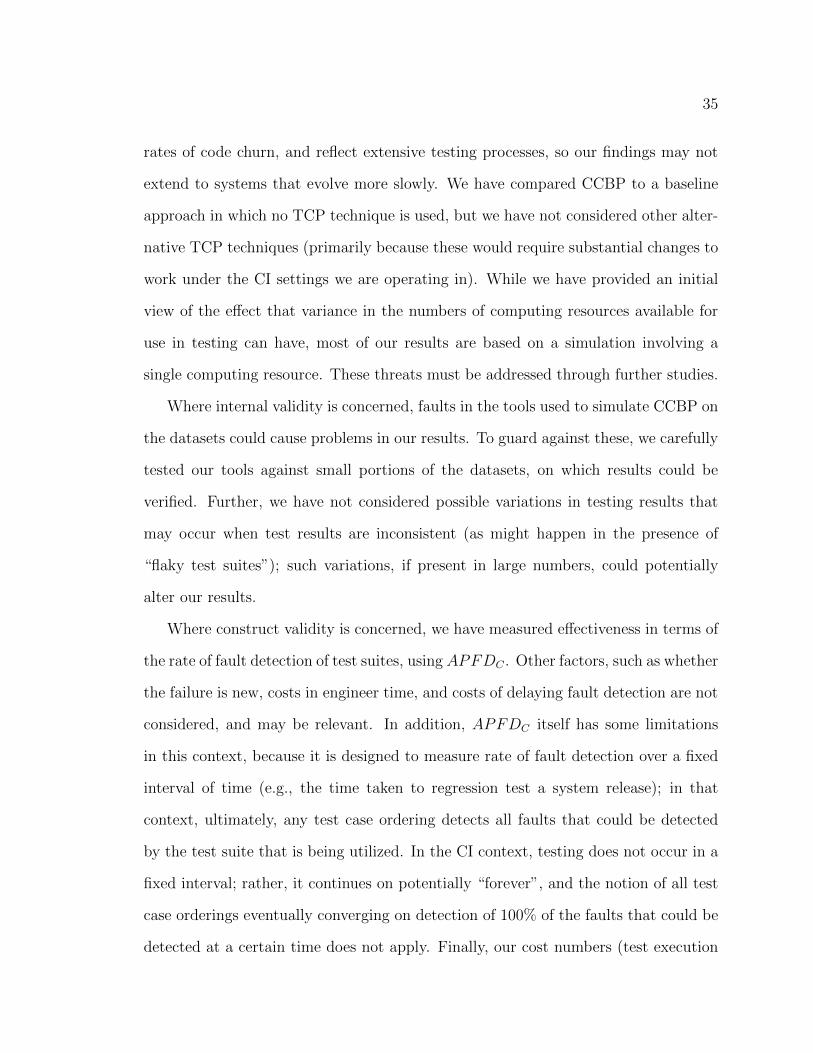
Figures 3.5, 3.6, and 3.7 summarize the results of applying CCBP to each dataset. In
each figure, the x-axis represents the percentage of testing time, the y-axis represents
the percentage of failing commits detected, and the three plotted lines correspond to
the original commit ordering, the inter-commit ordering produced by CCBP, and the
optimal commit ordering, respectively.
The figures reveal two distinct patterns. On the one hand, for GooglePre and
GooglePost, the space available for optimizing the commit order to improve the rate
of failure detection is clearly noticeable. The di↵erences between the original and
optimal orders are 20% and 25% for GooglePre and GooglePost, respectively. In
both cases CCBP, although still far from optimal, is able to provide gains on that

37
0 20 40 60 80 100
020
4060
8010
0
% of Time
% o
f Fai
ling
Com
mits
Exe
cute
d
●●●●●●●●●●●●●●●
●●●●●●●●●●●●●●●●●●●●●
●●●
●●●●●
●●●●●●
●●●●●
●●●●●
●●●●●●●●●●●●●●●●●●●●●●●●●●●●●●●●●●●●●●●●●
●
Original APFD = 50.4780%CCBP APFD = 62.0566%Optimal APFD = 76.3059%
Figure 3.6: APFD
C
on GooglePost
0 20 40 60 80 100
020
4060
8010
0
% of Time
% o
f Fai
ling
Com
mits
Exe
cute
d
●●●●●●●●●
●●●●●●
●●
●●●●
●
●
●●
●
●●●●●●
●●●●●
●●●●●●
●●●●●●●
●●●●●●●
●●●●●●●●
●●●●●●●
●●●●●
●●●
●●●●●●
●●●●●●●●●
●●●●●●
●
Original APFD = 55.4498%CCBP APFD = 55.4512%Optimal APFD = 55.4617%
Figure 3.7: APFD
C
on Rails
38
space over the original ordering, of 9% and 12%, respectively.
The space available for optimization in Rails, on the other hand, is almost non-
existent. The optimal and original orders overlap and their APFD
C
values do not
di↵er until the second decimal place. We conjecture that in this case the commit
arrival rate is low enough (Table 2.1, row 3), for the resources available, that commits
do not queue in large enough numbers to benefit from prioritization.
We explored this conjecture further by compressing the five months of Rails data
into one month (by changing all the months in all the date-type fields to March)
to cause artificial queuing of commits, and then applying CCBP. Figure 3.8 shows
the results (hereafter referred to as “Rails Compressed” data), and they support our
conjecture. Having compressed commit arrivals, there is now space for improving
the rate of failure detection and CCBP does provide gains of 6% over the original
order. This figure also illustrates an interesting situation: within the first 25% of the
testing time, the inter-commit order created by CCBP underperforms the original
order. This occurs because early in the process, CCBP does not have enough failure
history data to make informed prioritization decisions. This points to the previously
mentioned need for a “warm-up” period to collect enough history before applying
CCBP.
3.4.1 The “Continuous” in CCBP Matters
To better understand CCBP’s e↵ectiveness gains we performed a follow up exper-
iment. We designed an inter-commit prioritization technique that uses the same
heuristics as CCBP but prioritizes queued commits only once. The technique em-
ploys two queues: one for arriving commits and one for prioritized commits. When a
resource becomes available, the highest priority commit from the prioritized queue is
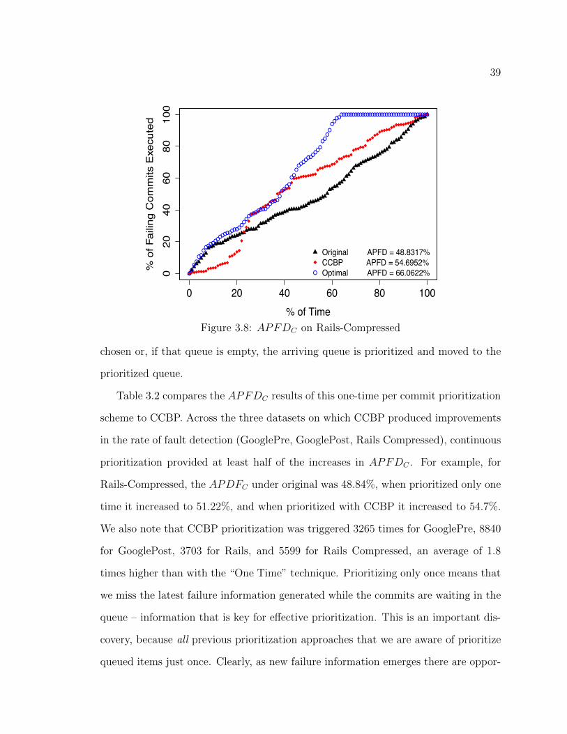
39
0 20 40 60 80 100
020
4060
8010
0
% of Time
% o
f Fai
ling
Com
mits
Exe
cute
d
●●●●●●
●●●
●●●●
●●●●●
●●●●●●●●●
●●●●●●
●●●
●●●●●
●●
●●●●●
●●●●
●●●
●
●●●●
●●●●
●●●●●●●●●●●●●●●●●●●●●●●●●●●●●●●●●●●●●
●
Original APFD = 48.8317%CCBP APFD = 54.6952%Optimal APFD = 66.0622%
Figure 3.8: APFD
C
on Rails-Compressed
chosen or, if that queue is empty, the arriving queue is prioritized and moved to the
prioritized queue.
Table 3.2 compares the APFD
C
results of this one-time per commit prioritization
scheme to CCBP. Across the three datasets on which CCBP produced improvements
in the rate of fault detection (GooglePre, GooglePost, Rails Compressed), continuous
prioritization provided at least half of the increases in APFD
C
. For example, for
Rails-Compressed, the APDF
C
under original was 48.84%, when prioritized only one
time it increased to 51.22%, and when prioritized with CCBP it increased to 54.7%.
We also note that CCBP prioritization was triggered 3265 times for GooglePre, 8840
for GooglePost, 3703 for Rails, and 5599 for Rails Compressed, an average of 1.8
times higher than with the “One Time” technique. Prioritizing only once means that
we miss the latest failure information generated while the commits are waiting in the
queue – information that is key for e↵ective prioritization. This is an important dis-
covery, because all previous prioritization approaches that we are aware of prioritize
queued items just once. Clearly, as new failure information emerges there are oppor-
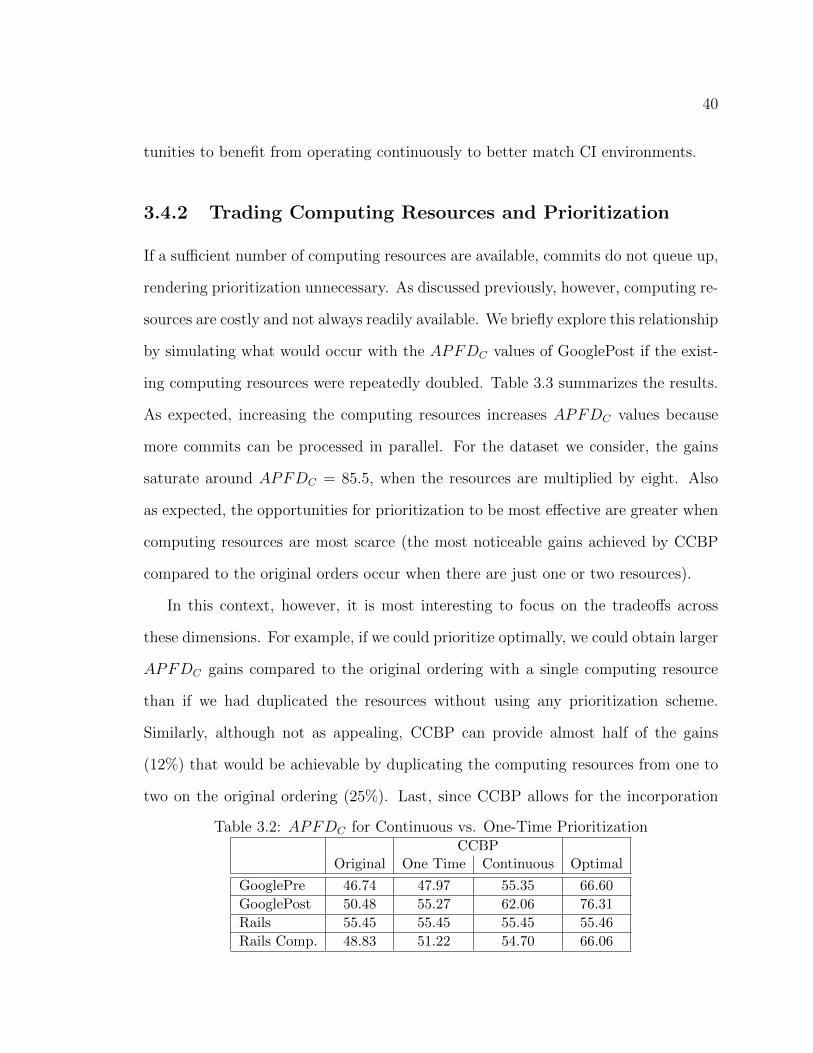
40
tunities to benefit from operating continuously to better match CI environments.
3.4.2 Trading Computing Resources and Prioritization
If a su�cient number of computing resources are available, commits do not queue up,
rendering prioritization unnecessary. As discussed previously, however, computing re-
sources are costly and not always readily available. We briefly explore this relationship
by simulating what would occur with the APFD
C
values of GooglePost if the exist-
ing computing resources were repeatedly doubled. Table 3.3 summarizes the results.
As expected, increasing the computing resources increases APFD
C
values because
more commits can be processed in parallel. For the dataset we consider, the gains
saturate around APFD
C
= 85.5, when the resources are multiplied by eight. Also
as expected, the opportunities for prioritization to be most e↵ective are greater when
computing resources are most scarce (the most noticeable gains achieved by CCBP
compared to the original orders occur when there are just one or two resources).
In this context, however, it is most interesting to focus on the tradeo↵s across
these dimensions. For example, if we could prioritize optimally, we could obtain larger
APFD
C
gains compared to the original ordering with a single computing resource
than if we had duplicated the resources without using any prioritization scheme.
Similarly, although not as appealing, CCBP can provide almost half of the gains
(12%) that would be achievable by duplicating the computing resources from one to
two on the original ordering (25%). Last, since CCBP allows for the incorporation
Table 3.2: APFD
C
for Continuous vs. One-Time PrioritizationCCBP
Original One Time Continuous Optimal
GooglePre 46.74 47.97 55.35 66.60
GooglePost 50.48 55.27 62.06 76.31
Rails 55.45 55.45 55.45 55.46
Rails Comp. 48.83 51.22 54.70 66.06
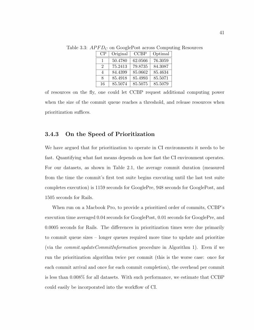
41
Table 3.3: APFD
C
on GooglePost across Computing ResourcesCP Original CCBP Optimal
1 50.4780 62.0566 76.3059
2 75.2413 79.8735 84.3087
4 84.4399 85.0662 85.4634
8 85.4918 85.4993 85.5071
16 85.5074 85.5075 85.5079
of resources on the fly, one could let CCBP request additional computing power
when the size of the commit queue reaches a threshold, and release resources when
prioritization su�ces.
3.4.3 On the Speed of Prioritization
We have argued that for prioritization to operate in CI environments it needs to be
fast. Quantifying what fast means depends on how fast the CI environment operates.
For our datasets, as shown in Table 2.1, the average commit duration (measured
from the time the commit’s first test suite begins executing until the last test suite
completes execution) is 1159 seconds for GooglePre, 948 seconds for GooglePost, and
1505 seconds for Rails.
When run on a Macbook Pro, to provide a prioritized order of commits, CCBP’s
execution time averaged 0.04 seconds for GooglePost, 0.01 seconds for GooglePre, and
0.0005 seconds for Rails. The di↵erences in prioritization times were due primarily
to commit queue sizes – longer queues required more time to update and prioritize
(via the commit.updateCommitInformation procedure in Algorithm 1). Even if we
run the prioritization algorithm twice per commit (this is the worse case: once for
each commit arrival and once for each commit completion), the overhead per commit
is less than 0.008% for all datasets. With such performance, we estimate that CCBP
could easily be incorporated into the workflow of CI.
42
3.4.4 On the E↵ect of Wf
Selection
a key parameter in Algorithm 1. Previous studies have explored the impact of dif-
ferent window sizes defined in terms of “time since the last observed failure” [15]
and reasoned that if the selected W
f
is too small, prioritization may not be sensitive
enough to relevant failures. Previous work also showed that if this window is too
large, too many test cases would have failed within the window, diluting the value of
the most recent failures and reducing the opportunities for e↵ective prioritization.
Given this potential range of e↵ects and the fact that we are operating at the
commit level, we decided to again explore a range of failure window sizes in terms
of the number of commits. To our surprise, we found that at the commit level the
approach was more robust to the choice of W
f
. More precisely, failure windows
between 10 and 500 commits achieved similar results.
Despite this finding, the reason for choosing large enough windows still holds.
We observe that when test suites fail, they tend to do so in spurts. Windows of
commits large enough to contain those spurts are e↵ective. Figure 3.9 illustrates
this for GooglePost. In the figure, the x-axis corresponds to commits ids, the y-axis
corresponds to test suite ids, and the circles indicate when a test suite failed. As
noted earlier, a small percentage of test suites fail, but in the figure we can also see
that, for the original commit ordering, failures on a given test suite usually occur in
small clusters (sequences of points for a given test suite across commits). As long as
W
f
is as large as most of those clusters (Wf
� 10), then the prioritization scheme
functions e↵ectively. Less intuitive is the notion that having much larger windows (of
up to 500 commits) does not negate the benefits of the approach. We believe this is
due to the small portion of test suites that exhibit failures (10% to 20% across the
datasets). With such a failure rate, larger windows do not result in a major influx
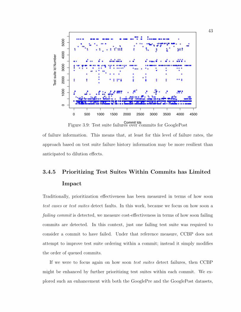
43
●●●●●
●●●
●
●
●
●●●●●●●●●●●●●●●●●●
●
●●●●
●
●●●
●
●
●
●
●
●
●●●●●
●
●
●
●●●
●●
●
●
●●●●●●●●●●●●●
●
●
●
●●●
●●
●
●
●●
●●
●●
●
●
●●
●
●●●●●●●
●
●
●
●
●●●●●●
●
●
●
●
●
●
●
●
●●●
●
●●
●
●
●
●●●●
●
●●
●●●
●
●●
●
●
●●●●
●
●
●
●●
●
●●●
●
●●
●●
●●
●
●
●●
●
●
●
●●●
●
●●
●●
●●●
●
●
●
●
●
●
●
●
●
●
●
●●
●
●
●
●
●
●
●
●
●
●●
●●
●●
●●●●
●●
●
●●●●●
●●●
●●
●
●●
●
●
●
●●●
●
●
●●
●
●●
●●●●●●
●
●
●
●
●●●
●
●●
●●●
●
●●●●
●
●●●
●
●●
●
●
●
●
●
●●●●●●
●
●●●●●
●
●
●●
●
●●
●
●●●●●●●●●
●
●
●●●
●
●
●
●●
●
●●●
●●●
●
●
●
●●
●
●
●
●●●●●●●●●●●●●●●●●●●
●
●●●
●
●
●
●
●
●●
●●●●●●●
●
●●●
●●
●●●
●
●●
●●●
●
●●●
●●●
●
●●●
●●
●
●
●●
●
●
●●
●●
●
●●●●●
●
●
●
●●
●●●●
●
●●●●
●
●●●
●
●
●●
●
●
●
●●
●
●
●
●
●
●●
●●
●●●
●
●●●
●●●●
●●●
●●●●
●●
●●
●
●
●
●
●
●●
●●●
●●●●●●●
●●
●●
●●
●
●●●
●
●●
●
●
●●
●●
●●●●●●●●●
●●
●
●●●●●
●
●
●
●●●●
●●
●
●
●●
●●●●●
●
●
●●
●●
●
●
●
●
●
●
●
●
●●●●●●●●●●●●
●
●●●●
●
●●
●
●
●
●
●●
●●●
●●
●●●
●●●
●
●
●●
●
●
●●
●●●
●●
●●●●●●
●
●●●
●●●●●●
●●
●●●
●●●●●
●
●
●
●
●
●●●
●
●●●●●●
●●
●
●
●
●
●
●●●●●●●●●●●●●●●●●●●
●
●●
●
●●
●●●
●
●
●
●
●
●●●
●
●●●
●
●
●
●
●
●●●●●●●
●
●
●
●●●●●●●●●●●●●●●●
●
●●
●
●●●
●
●●●●
●
●●●●●●
●●
●●
●●●
●
●●●●
●●●
●
●●●●
●●●●●●
●
●
●
●
●●●
●
●
●
●
●
●●●●●
●●
●
●
●
●●
●
●●
●●
●
●●
●
●
●
●●●●●
●●
●
●
●
●●
●
●
●
●●
●
●●
●
●
●
●
●
●
●●
●●●
●
●
●●
●●
●
●●●
●
●●
●
●●●●●
●●
●●●
●
●
●
●●
●
●●●
●
●
●
●●●●●●●
●
●●●●●●●
●
●●
●
●●●●●●
●●●
●●●●●●
●●
●
●●
●
●●
●●
●●●●
●
●
●
●
●●
●●●
●
●
●
●●
●●●●●●
●
●●●
●●
●
●
●●●●●●●
●●●●●●
●●
●
●
●●●
●
●●●
●
●
●●●●●●
●●●
●●
●
●
●●●
●
●●
●●●
●●●●●●
●●●
●●
●
●
●
●●
●
●
●
●●
●
●●●●
●
●
●●
●●●
●
●●
●●●
●●
●●●●●●●●●●●●●●●
●
●
●
●
●
●●
●
●
●
●●●●●●●●●●●●●●●●●●●●●
●
●●●
●
●
●●
●
●
●●
●
●●●●●●●●●
●
●●●
●
●●
●
●
●
●●●●
●●
●
●●●
●●●●
●●●
●●●
●
●●●●●●
●
●●
●
●
●
●
●●●
●●●●
●
●●●
●
●●
●●●●
●
●
●●●●●
●
●
●
●●
●
●●●●●●●●●●●●●●●●
●
●
●
●
●●●
●
●
●
●
●
●
●
●●●●●●●●●
●
●●●●●●●
●●
●
●
●●●●●
●
●●●●
●
●
●●●●●
●●●●
●
●
●
●
●●●
●
●
●
●
●●
●
●
●
●●●●●●●●●●●●●●●●●●
●
●
●●●
●
●
●●●●●●●●●
●
●
●
●●●●●●●●●●●●●●●●●●●
●●
●
●
●
●
●●●
●
●
●
●
●●
●
●●
●
●
●
●
●
●●
●
●
●
●●●
●●●
●
●
●
●
●
●
●
●
●●
●
●
●
●
●●●
●●●●●●●●●●
●
●●
●
●●●
●●●●●●●●●●●●●●●●●●●
●
●
●
●
●●
●
●●●
●
●●
●
●
●
●●●●
●●●
●
●
●●●●●
●
●●
●
●●●●●●●●●●
●●
●
●
●●●
●
●●
●●
●
●●
●
●●●
●
●●●●
●
●●●●●
●●
●●
●
●●
●●
●●
●
●
●●
●●●●
●
●●●
●
●●●●●
●
●●●●
●●●
●●●
●●
●
●
●●●●
●
●
●
●●
●
●
●●
●●
●
●●
●
●
●
●
●
●
●●
●
●
●●●●●●
●
●
●●
●
●
●●●
●●●
●
●●●●●
●
●●
●●
●
●
●●●
●
●●●●●
●
●●
●●●●●
●●●
●
●
●●
●
●
●
●
●●●
●●●
●
●
●
●
●●
●●
●●●
●●
●●●
●
●●
●
●●●●●
●
●●
●
●●
●●●●●●●●●
●
●●
●
●
●
●●●●●●●●●
●
●
●
●●●
●●●
●
●
●
●
●
●
●
●
●
●
●
●
●
●●●
●
●
●●
●●
●●
●
●●●●
●
●
●
●
●
●
●
●●●●●●●●●●●●●●●●●●
●
●●●
●
●●●
●●
●
●
●●●●●●●
●●●
●
●
●
●
●
●
●
●
●●●
●●●
●
●
●●●●
●
●●●●
●●●
●
●
●●●
●
●
●●●●●
●●●●
●
●
●
●
●
●
●
●
●●●●●
●
●
●
●●●
●
●●
●
●
●
●●
●●●●●●●
●●
●●
●
●●●
●
●●●●●
●
●●●
●
●●●
●
●
●
●●
●
●
●
●●●
●●●●●●
●
●●
●●●
●●
●
●
●
●
●●
●
●
●●●●●●●
●●●
●
●●
●●●●
●
●
●
●
●●
●●●
●●
●●
●●●●
●
●
●●
●
●●
●
●●●
●●
●
●●●
●
●●
●●
●●
●
●
●
●
●●●●
●●●●●●●●●●●●●●●●●●●●●●●●●●●●●●●●●●●●●●●●●●●●●●●●●●●●●●●●●●●●●●●●●●●●●●●●●●●●●●●●●●●●●●●●●●●●●●●●●●●●●●●●●●●●●●●●●●●●●●●●●●●●●●●●●●●●●●●●●●●●●●●●●●●●●●●
●
●
●
●
●
●●
●
●●●●
●
●●
●●●●●●●●●●●●●●●●●●●●●
●●●●
●●●●●●●●●●●●●●●●●●●●●●●●●●●●●●●●●●●●●●●●●●●●●●●●●●●●●●●●●●●●●●●●●●●●●●●●●●●●●●●●●●●●●●●●●●●●●●●●●●●●●●●●●●●●●●●●●●●●●●●●●●●●●●●●●●
●
●●●●●●●●●●●●●●●●●●●●●●●●●●●●●●●●●●●●●●●●●●●●●●●●●●●●●●●●●●●●●●●●●●●●●●●●●●●●●●●●●●●●●●●●●●●●●●●●●●●●●●●●●●●●●●●●●●●●●●●●●●●●●●●●●●●●●●●●●●●●●●●●●●●●●●
●●●●●●●●●●●●●●
●●●●●●●●●●●●●●●●●●●●●●●●●●●●●●●●●●●●●●●●●●●●●●●●●●●●●●●●●●●●●●●●●●●●●●●●●●●●●●●●●●●●●●●●●●●●●●●●●●●●●●●●●●●●●●●●●●●●●●●●●●●●●●●●●●●●●●●●●●●●●●●●●●●●●●●
●●●
●●●●●●●●●●●●●●●●●●●
●●●
●●●●●●●●●●●●●●●●●●●●●●●●●●●●●●●●●●●●●●●●●●●●●●●●●●●●●●●●●●●●●●●●●●●●●●●●●●●●●●●●●●●●●●●●●●●●
●
●●●
●●●●●●●●●●
●
●
●●●●●●●●●●
●●
●
●
●
●
●●●●●●●
●
●●●
●●●●●●●●●●●●●●●●●●●●●●●●●●●●●●●●●●●●●●●●●●●●●●●●●●●●●●●●●●●●●●●●●●●●●●●●●●●●●●●●●●●●●●●●●●●●●●●●●●●●●●●●●●●●●●●●●●●●●●●●●●●●●●●●●●●●●●●●●●●●●●●●●●●●●●●●●●●●●●●●●●●●●●●●●●●●●●●●●●●●●●●●●●●●●●●●●●●●●●●●●●●●●●●●●●●●●●●●●●●●●●●●●●●●●●●●●●●●●●●●●●●●●●●●●●●●●●●●●●●●●●●●●●●●●●●●●●●●●●●●●●●●●●●●●●●●●●●●●●●●●●●●●●●●●●●●●●●●●●●●●●●●●●●●●●●●●●●●●●●●●●●●●●●●●●●●●●●
●●
●●●●●●●●●●●●●●●●●●●
●
●●●●●●●●●●●●●●●●●●●●●●●●●●●●●●●●●●●●●●●●●●●●●●●●●●●●●●●●●●●●●●●●●●●●●●●●●●●●●●●●●●●●●●●●●●●●●●●●●●●●●●●●●●●●●●●●●●●●●●●●●●●●●●●●●●●●●●●●●●●●●●●●●●●●●●●●●●●●●●●●●●●●●●●●●●●●●●●●●●●●●●●●●●●●●●●●●●●●●●●●●●●●●●●●●●●●●●●●●●●●●●●●●●●●●●●●●●●●●●●●●●●●●●●●●●●●●●●●●●●●●●●●●●●●●●●●●●●●●●●●●●●●●●●●●●●●●●●●●●●●●●●●●●●●●●●●●●●●●●●●●●●●●●●●●●●●●●●●●●●●●●●●●●●●●●●●●●●●●●●●●●●●●●●●●●●●●●●●●●●●●●●●●●●●●●●●●●●●●●●●●●●●●●●●●●●●●●●●●●●●●●●●●●●●●●●●●●●●●
●
●●●
●●●●●●●●●●●●●●●●●●●●●●●●●●●●●●●●●●
●
●
●
●●●●●●
●●●
●●●
●
●●●●●●●
●
●●●●●●
●
●●
●●●●
●●●
●
●
●●●
●●●●●●
●
●
●
●
●
●●
●
●●●●●●●●●●●●●●●●●●
●●
●●●
●
●
●●
●●●●●●●
●
●●●●●●
●
●
●●●●
●●
●●●
●
●
●●●●●●
●●●
●
●●
●●
●
●●●●●●●●
●
●
●
●
●
●●
●
●●
●●●
●●●
●
●●
●
●●
●
●
●
●
●●
●●●
●
●
●●●
●●
●
●
●
●
●●
●
●
●
●●
●
●
●●●
●
●●
●
●●●●
●
●
●
●
●●
●
●
●
●
●●●
●●
●●
●●●
●
●
●
●
●
●●
●●
●●
●
●
●
●
●●
●
●●
●
●●●●●●●●●●●●●●
●●
●
●●●
●
●●
●
●●
●●
●
●
●
●●
●
●
●
●●●
●
●
●
●
●
●●
●
●●●
●●
●●●●
●
●
●
●
●
●
●
●
●
●●●
●●
●
●
●
●
●
●
●
●●
●
●
●
●
●
●
●●●
●●
●●
●●
●
●
●
●
●
●●●●
●
●●●●●●
●
●
●
●●●●●●●●
●
●●●●
●
●●
●
●
●
●
●
●
●
●
●
●●●●●●●●●●●●●●●●●●●●
●●
●
●
●
●●●
●
●
●
●●●●●●●●●
●
●●●●
●
●
●
●●
●●●
●
●●
●●
●
●
●●●●
●
●
●●●●
●●●●●
●
●
●
●●●●●
●●
●●●
●●
●
●●●
●●●●
●
●
●
●
●
●●
●
●
●●
●
●
●●
●
●
●●
●●
●●●
●●
●
●
●●
●
●●●
●
●
●
●●●
●●●
●
●
●
●
●
●
●
●●
●●
●
●
●
●●●
●
●●●
●
●
●●
●
●
●●
●
●●
●
●●
●
●
●●●
●
●
●●
●●
●●●
●
●
●●
●
●
●●
●
●●
●●
●●●
●
●
●●
●●●●
●
●
●
●●●●
●
●
●
●
●●
●
●
●
●●●●
●
●
●
●
●●●
●
●●●
●●
●●●
●
●
●●
●
●●●
●
●
●
●
●
●
●
●
●
●●●●●●●●●●●●●●●●
●
●
●●
●
●●●
●
●
●●
●
●
●●
●●●
●
●●●●●
●
●●●●
●
●●●
●●●●●●●●
●●●
●
●
●●●
●●
●
●
●●
●●●
●●
●●●
●
●●●●●●
●●
●●
●
●●●
●
●
●●
●
●
●●
●●
●
●
●
●
●●
●●
●●
●
●●●●●●●●
●
●
●●●●●
●
●●●●●●●●●
●
●
●
●●
●
●●●●
●
●
●
●
●●●●●
●
●
●●●
●
●●●
●●●
●
●
●●●
●●●
●●
●
●
●
●
●
●●●●●●
●
●●●
●
●
●●
●
●●●●
●
●●
●
●
●
●●●
●
●●●●
●●●
●
●●●
●●●
●●●
●
●●
●●●
●
●
●
●
●●
●
●●
●●●
●●●
●
●●●
●
●●
●
●●
●●
●
●●●
●
●
●●
●
●
●●
●
●●
●
●
●●
●●●●●
●●●●●
●●
●
●
●
●
●●
●
●
●●
●●●●●●●●●
●
●
●●
●
●
●
●●●
●
●
●
●●
●●●
●
●
●
●●●●●●●
●
●
●●
●
●
●●●●●●●●●●●●●●●●●●●●
●
●
●●●
●
●
●●●●
●
●
●
●
●
●
●
●●
●
●
●
●●●●●
●
●
●
●
●
●
●
●
●
●
●●●●●●●●●●●●●●●●
●
●
●
●●●
●
●
●
●●●●●●
●
●
●
●
●●●●●●●●●●●●●●
●●
●●
●
●
●
●
●
●
●
●●●●●●●●●●●●●●●●●
●●●
●●●
●
●●●●●●●●
●
●●●●●●●
●
●●●●●●●●
●
●●●●●●●●
●
●
●
●
●
●●
●●
●
●●
●●●●
●●●●●●●●
●●
●●●
●
●
●●●●
●
●●●
●
●
●●●●●●
●
●
●
●
●
●●
●
●
●
●
●●●●
●
●●●
●
●
●
●
●
●
●
●
●
●
●
●
●
●
●●
●
●●●●●
●
●
●
●
●
●
●●●●
●●
●
●●●
●
●●
●
●
●
●
●●●
●
●
●●●
●
●
●
●
●●
●
●
●
●
●
●
●
●
●
●
●
●
●
●
●
●
●●●●●
●
Commit Ids
Test
sui
te Id
Num
ber
0 500 1000 1500 2000 2500 3000 3500 4000 4500
010
0020
0030
0040
0050
00
Figure 3.9: Test suite failures over commits for GooglePost
of failure information. This means that, at least for this level of failure rates, the
approach based on test suite failure history information may be more resilient than
anticipated to dilution e↵ects.
3.4.5 Prioritizing Test Suites Within Commits has Limited
Impact
Traditionally, prioritization e↵ectiveness has been measured in terms of how soon
test cases or test suites detect faults. In this work, because we focus on how soon a
failing commit is detected, we measure cost-e↵ectiveness in terms of how soon failing
commits are detected. In this context, just one failing test suite was required to
consider a commit to have failed. Under that reference measure, CCBP does not
attempt to improve test suite ordering within a commit; instead it simply modifies
the order of queued commits.
If we were to focus again on how soon test suites detect failures, then CCBP
might be enhanced by further prioritizing test suites within each commit. We ex-
plored such an enhancement with both the GooglePre and the GooglePost datasets,

44
measuring APFD
C
over the percentage of test suites executed. We prioritized with
three techniques: (1) CCBP as defined, (2) CCBP with intra-commit prioritization of
test suites, and (3) the original order with intra-commit prioritization of test suites.
For the GooglePre dataset, we found that neither technique 2 nor technique 3 pro-
vided much improvement over CCBP in terms of e↵ectiveness. We attribute this to
the large proportion of distinct failing test suites in this dataset, which makes failure
prediction at the test suite level ine↵ective (even though when failures are aggregated
at the commit level they provide noticeable gains). For the GooglePost dataset the
APFD
C
for CCBP was 17% greater than for technique 3, and technique 2 provided
only a 0.5% gain, rendering the contribution of intra-commit prioritization marginal.
3.4.6 Delays in Detecting Failing Commits
Although the APFD
C
metric measures the rate of fault detection, it can be useful
and more intuitive to compare techniques’ cost-e↵ectiveness in terms of the reduc-
tion in delays to detect failing commits under the di↵erent orderings. It is these
reductions in delays that allow prioritization to provide potential advantages to de-
velopers. To capture the notion of delays, we accumulated failing commit time di↵er-
ences between CCBP and the original commit order. More specifically, we compute
Pn
f=1(commit
f
.startT ime+commit
f
.duration/2) (this last term assumes an average
time for a commit to fail) over all the failing commits f under CCBP and the original
order, and normalize that by the number of failing commits in each artifact (267, 1022,
and 574 failing commits for GooglePre, GooglePost, and Rails respectively as per Ta-
ble 2.1, row 2). The findings are consistent with those reported earlier. On average,
CCBP reduces the delays in detecting failing commits by 46 hours for GooglePre, 135
hours for GooglePost, and 69 hours for Rails Compressed, while achieving no reduc-
45
tions for Rails. These delay reductions, although significant, are in computing hours,
and as such, can be reduced by using multiple computing resources as described pre-
viously. Still, as we argued earlier, computing resources come with a cost and CCBP
reduces feedback time without incurring additional costs. Since our dataset does not
provide information on resource availability we leave further assessment of the impact
of delays on developer’s time for future work.
3.5 Summary
We have presented a novel algorithm, CCBP, for increasing the rate of fault detection
in CI environments via prioritization. Unlike prior algorithms, CCBP prioritizes at
the level of commits, not test cases, and it does so continuously as commits arrive
or complete. CCBP is lightweight and operates quickly, allowing it to be su�ciently
responsive in CI environments. Our empirical study shows that after prioritization,
our technique can e↵ectively detect failing commits earlier.
46
Chapter 4
Test Suite Level Selection for CI
As we noted in Chapter 1, most existing RTS techniques utilize instrumentation to
track the code executed by test cases, and then analyze code changes and relate
them to these test executions. Those techniques cannot be cost-e↵ectively applied
in CI environments. Alternatively, we could utilize the test suites’ execution history
information for prediction. In this chapter, we provide our new algorithms that do
this, and the results and analysis of our empirical study of those algorithms.
4.1 Motivation
There are two key motivations for this work. First, the RTS approach for CI presented
by Elbaum et al. [15] was promising, but the windows that that technique relies on
are measured in terms of time, which is limited when the rate of test suite arrival
varies. Second, existing RTS techniques for CI only utilize test suites’ execution
status history to do selection, but fail to consider information about “pass to fail”
transitions.
As noted in Chapter 1, a wide range of RTS techniques have been developed and
47
studied, and could potentially be applied in the CI context. In practice, however,
existing techniques will not su�ce. Codebases that are under continous integra-
tion undergo frequent changes; the Google codebase, for example, undergoes tens of
changes per minute [21]. Most existing RTS techniques utilize instrumentation to
track the code executed by test cases, and then analyze code changes and relate them
to these test executions. The rate of code churn in the Google codebase, however,
is quite large, and this can cause code instrumentation results to quickly become
inaccurate. In such situations, keeping coverage data up to date is not feasible [11].
Elbaum et al. [15] provided a lightweight RTS technique for CI which utilizes two
windows based on time (we refer this as the TB technique) to track how recently test
suites have been executed and revealed failures, and use this information to select a
subset of test suites for execution. This technique is based on the conjecture that
an RTS approach that selects test suites based on some “failure window” might be
cost-e↵ective in continuous testing. This is because it has long been suggested, in
the testing literature, that some test cases (or test suites) are inherently better than
others at revealing failures [29]. In an evolving system, test suites that have failed on
a recent version are in some ways “proxies” for code change – they target code that is
churning. This technique defines an Execution Window (We
) and a Failure Window
(Wf
) based on time. Essentially, if We
is defined to be te
hours, and W
f
is defined to
be t
f
hours, then when considering test suite T , if T has failed within t
f
hours, or if
T has not been executed within t
e
hours, T will be selected. New test suites are also
necessarily selected.
Table 4.1 provides an example that illustrates how TB works. Because TB con-
siders a given test suite in isolation from others, the table provides data on just a
single test suite t1, with each row providing data on arrivals of that test suite into the
testing queue, in turn, from top to bottom. Column 3 (“Status”) indicates whether
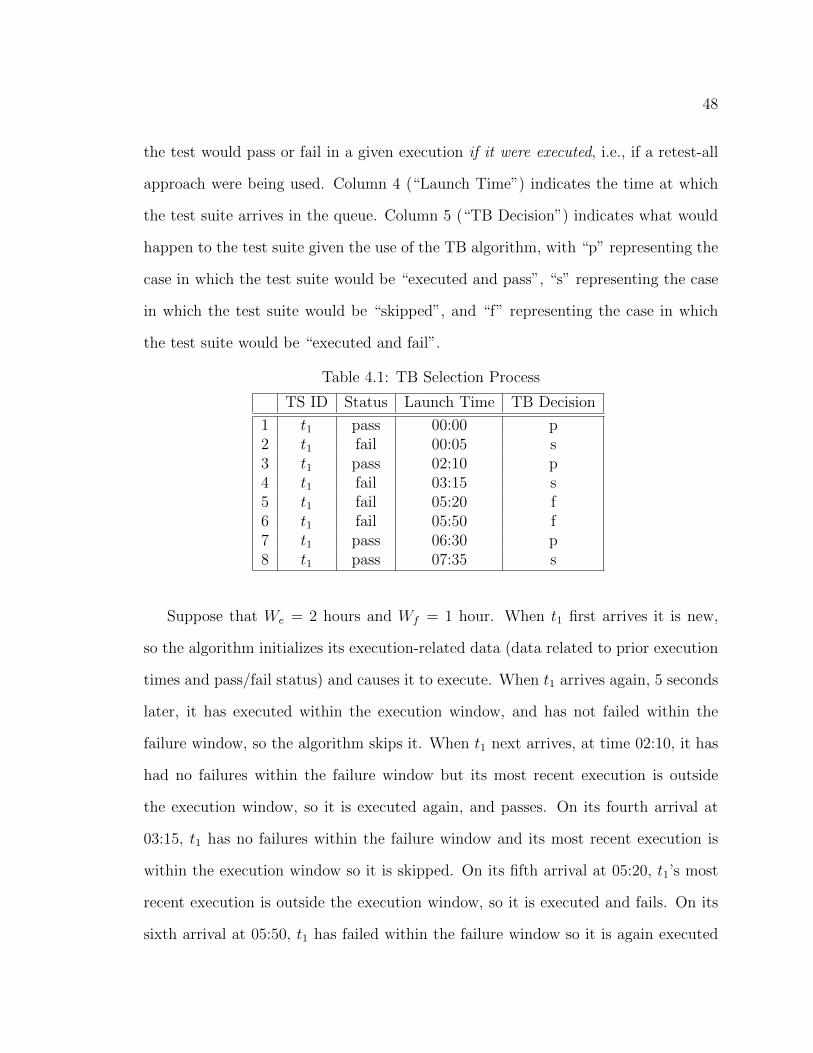
48
the test would pass or fail in a given execution if it were executed, i.e., if a retest-all
approach were being used. Column 4 (“Launch Time”) indicates the time at which
the test suite arrives in the queue. Column 5 (“TB Decision”) indicates what would
happen to the test suite given the use of the TB algorithm, with “p” representing the
case in which the test suite would be “executed and pass”, “s” representing the case
in which the test suite would be “skipped”, and “f” representing the case in which
the test suite would be “executed and fail”.
Table 4.1: TB Selection Process
TS ID Status Launch Time TB Decision
1 t1 pass 00:00 p2 t1 fail 00:05 s3 t1 pass 02:10 p4 t1 fail 03:15 s5 t1 fail 05:20 f6 t1 fail 05:50 f7 t1 pass 06:30 p8 t1 pass 07:35 s
Suppose that W
e
= 2 hours and W
f
= 1 hour. When t1 first arrives it is new,
so the algorithm initializes its execution-related data (data related to prior execution
times and pass/fail status) and causes it to execute. When t1 arrives again, 5 seconds
later, it has executed within the execution window, and has not failed within the
failure window, so the algorithm skips it. When t1 next arrives, at time 02:10, it has
had no failures within the failure window but its most recent execution is outside
the execution window, so it is executed again, and passes. On its fourth arrival at
03:15, t1 has no failures within the failure window and its most recent execution is
within the execution window so it is skipped. On its fifth arrival at 05:20, t1’s most
recent execution is outside the execution window, so it is executed and fails. On its
sixth arrival at 05:50, t1 has failed within the failure window so it is again executed
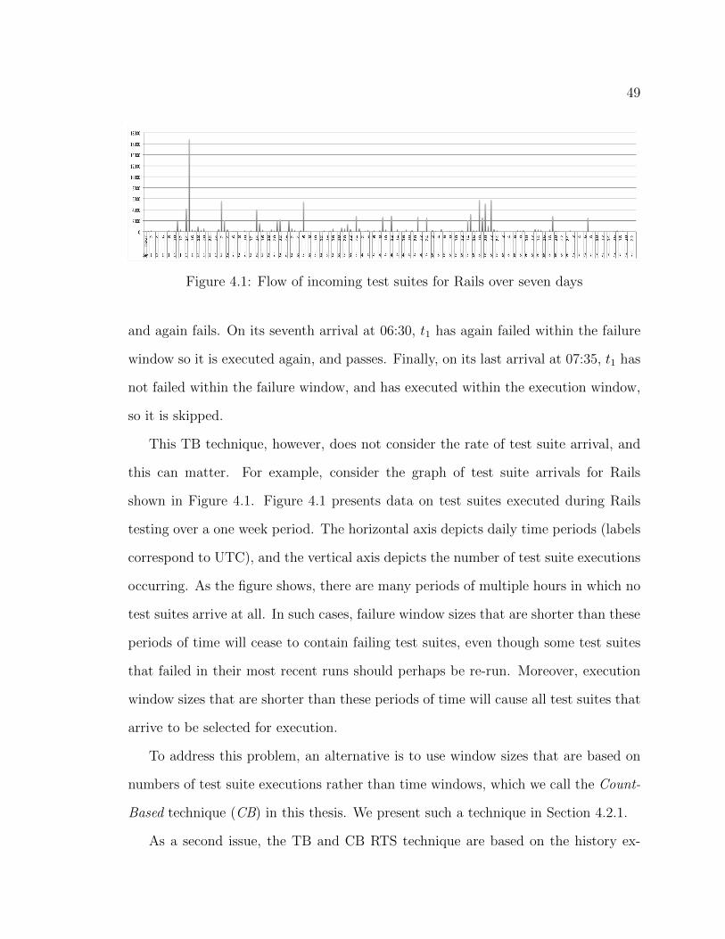
49
Figure 4.1: Flow of incoming test suites for Rails over seven days
and again fails. On its seventh arrival at 06:30, t1 has again failed within the failure
window so it is executed again, and passes. Finally, on its last arrival at 07:35, t1 has
not failed within the failure window, and has executed within the execution window,
so it is skipped.
This TB technique, however, does not consider the rate of test suite arrival, and
this can matter. For example, consider the graph of test suite arrivals for Rails
shown in Figure 4.1. Figure 4.1 presents data on test suites executed during Rails
testing over a one week period. The horizontal axis depicts daily time periods (labels
correspond to UTC), and the vertical axis depicts the number of test suite executions
occurring. As the figure shows, there are many periods of multiple hours in which no
test suites arrive at all. In such cases, failure window sizes that are shorter than these
periods of time will cease to contain failing test suites, even though some test suites
that failed in their most recent runs should perhaps be re-run. Moreover, execution
window sizes that are shorter than these periods of time will cause all test suites that
arrive to be selected for execution.
To address this problem, an alternative is to use window sizes that are based on
numbers of test suite executions rather than time windows, which we call the Count-
Based technique (CB) in this thesis. We present such a technique in Section 4.2.1.
As a second issue, the TB and CB RTS technique are based on the history ex-
50
ecution result (pass or fail status) of test suites’ executions. An advantage of these
result-based techniques is that, for any test suite, if a failure is detected only once, it
would be selected for execution again and again, and more failures could be detected.
Obviously, these result-based techniques could improve the detection of transitions
from “fail” to “fail”. However, these techniques do not consider that it can be much
more di�cult to detect an initial failure, which in another word, represents a “pass
to fail” transition.
The TB technique example in Table 4.1 helps motivate a technique that focuses
on “pass to fail” transitions. From this execution process, we can see that it is much
harder to detect a “pass to fail” transition (the 2nd and 4th test arrival) than a “fail to
fail” transition (the 6th arrival). If the test suite has detected a failure, then this test
suite will be executed again and again to check whether the problem leading to the
failure has been resolved. However, a new failure (from a “pass” to “fail” transition)
is detected based on W
e
. And if a new failure has been detected, the following failures
will be detected more easily.
In addition, as suggested earlier in Chapter 1, “pass to fail” transitions could
provide engineers with more information than just “pass to pass”,“fail to pass” or
“fail to fail” transitions.
Figure 4.2 shows “transition graphs” for Google Pre. In Figure 4.2, there are three
statuses, “new”, “pass” and “fail”, representing three test suite execution statuses
respectively. The directed edges represent the transitions from one status to another.
The numbers on the directed edges represent the percentages of certain transitions.
For example, the directed edge from “pass” to “fail” and the number 0.079 on the
edge indicates that in the Google Pre dataset, 0.079% of all transitions are “pass to
fail” transitions. By comparing the transition percentages, we can see that 99.246%
of transitions are “pass to pass” transitions, and 0.072% of transitions are “fail to
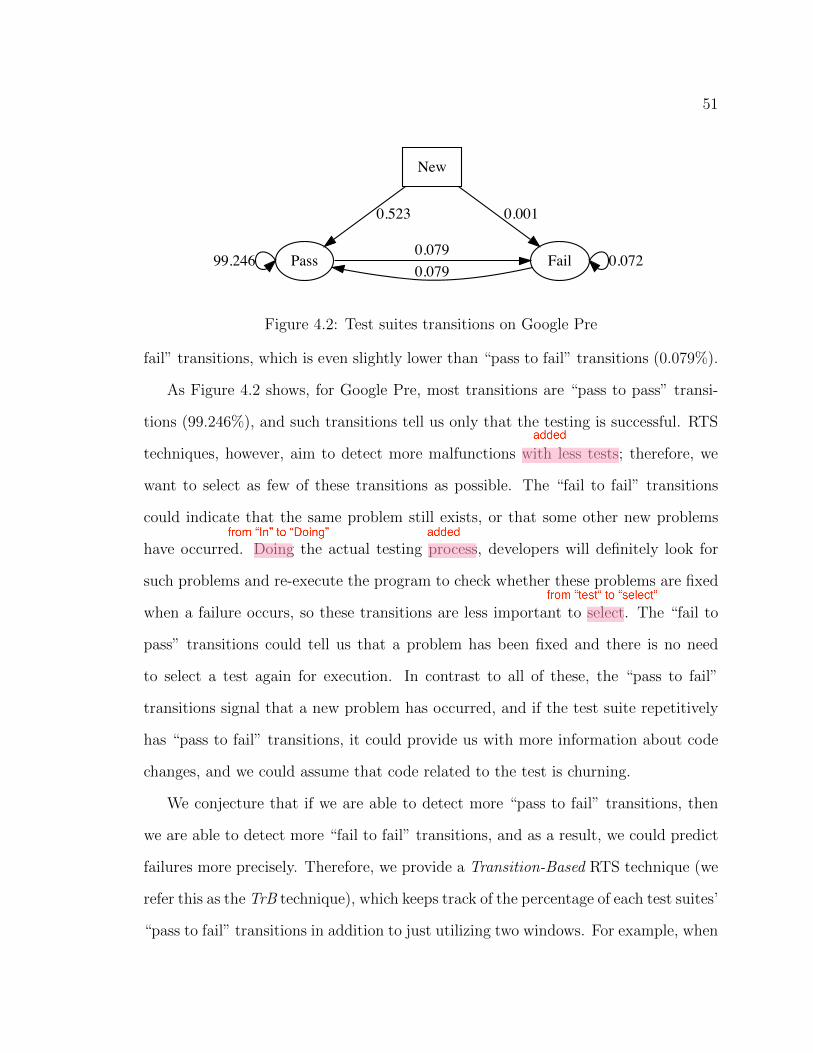
51
Pass99.246 Fail0.0790.079
0.072
New
0.523 0.001
Figure 4.2: Test suites transitions on Google Pre
fail” transitions, which is even slightly lower than “pass to fail” transitions (0.079%).
As Figure 4.2 shows, for Google Pre, most transitions are “pass to pass” transi-
tions (99.246%), and such transitions tell us only that the testing is successful. RTS
techniques, however, aim to detect more malfunctions with less tests; therefore, we
want to select as few of these transitions as possible. The “fail to fail” transitions
could indicate that the same problem still exists, or that some other new problems
have occurred. Doing the actual testing process, developers will definitely look for
such problems and re-execute the program to check whether these problems are fixed
when a failure occurs, so these transitions are less important to select. The “fail to
pass” transitions could tell us that a problem has been fixed and there is no need
to select a test again for execution. In contrast to all of these, the “pass to fail”
transitions signal that a new problem has occurred, and if the test suite repetitively
has “pass to fail” transitions, it could provide us with more information about code
changes, and we could assume that code related to the test is churning.
We conjecture that if we are able to detect more “pass to fail” transitions, then
we are able to detect more “fail to fail” transitions, and as a result, we could predict
failures more precisely. Therefore, we provide a Transition-Based RTS technique (we
refer this as the TrB technique), which keeps track of the percentage of each test suites’
“pass to fail” transitions in addition to just utilizing two windows. For example, when
52
deciding whether to execute a given test suite T that is being considered for execution,
the technique considers whether T has failed within the past Wf
test suite executions,
whether T has not been executed at all during the pastWe
test executions, or whether
T ’s percentage of “pass to fail” transitions is higher than a random number R, and
bases its selection on that. We present this technique in Section 4.2.2.
4.2 Approach
We now present our Count-Based technique (CB) and Transition-Based technique
(TrB) algorithms.
4.2.1 Count-Based RTS Approach
As mentioned in Section 4.1, windows based on numbers of test suite executions
could address the issues that arise when the rate of test suite arrival varies. The
CB approach utilizes the same method as the TB technique provided by Elbaum
et al. [15]. The only di↵erence is that the selection windows of the TB technique
are based on time, whereas the selection windows of the CB technique are based on
numbers of test suite executions.
Algorithm 2 presents the CB algorithm. In this case, instead of taking a test suite
T
i
and two time window sizes as parameters, the algorithm takes a test suite T
i
and
two integer parameters, exeWindowSize and failWindowSize, corresponding to the
sizes of the execution window and failure window, and measured in terms of numbers
of test suites. In this work, we set the parameters to specific constant values, but in
practice they could be adjusted based on changing conditions.
Lines 5-8 initialize data for new test suites. Whenever a new test suite arrives
(a new test suite suite is a distinct test suite that hasn’t been executed before),
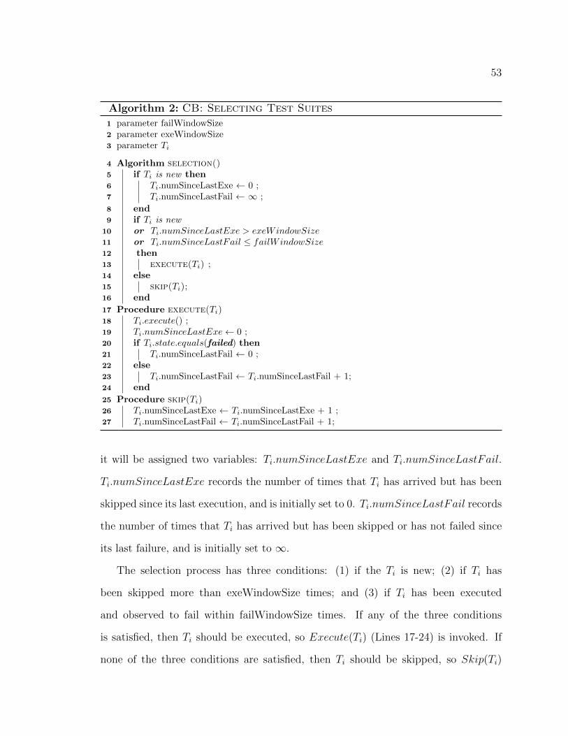
53
Algorithm 2: CB: Selecting Test Suites
1 parameter failWindowSize2 parameter exeWindowSize3 parameter Ti
4 Algorithm selection()
5 if Ti is new then
6 Ti.numSinceLastExe 0 ;7 Ti.numSinceLastFail 1 ;
8 end
9 if Ti is new
10 or Ti.numSinceLastExe > exeWindowSize
11 or Ti.numSinceLastFail failWindowSize
12 then
13 execute(Ti) ;
14 else
15 skip(Ti);
16 end
17 Procedure execute(Ti)
18 Ti.execute() ;19 Ti.numSinceLastExe 0 ;20 if Ti.state.equals(failed) then21 Ti.numSinceLastFail 0 ;22 else
23 Ti.numSinceLastFail Ti.numSinceLastFail + 1;24 end
25 Procedure skip(Ti)
26 Ti.numSinceLastExe Ti.numSinceLastExe + 1 ;27 Ti.numSinceLastFail Ti.numSinceLastFail + 1;
it will be assigned two variables: T
i
.numSinceLastExe and T
i
.numSinceLastFail.
T
i
.numSinceLastExe records the number of times that Ti
has arrived but has been
skipped since its last execution, and is initially set to 0. Ti
.numSinceLastFail records
the number of times that Ti
has arrived but has been skipped or has not failed since
its last failure, and is initially set to 1.
The selection process has three conditions: (1) if the T
i
is new; (2) if T
i
has
been skipped more than exeWindowSize times; and (3) if T
i
has been executed
and observed to fail within failWindowSize times. If any of the three conditions
is satisfied, then T
i
should be executed, so Execute(Ti
) (Lines 17-24) is invoked. If
none of the three conditions are satisfied, then T
i
should be skipped, so Skip(Ti
)
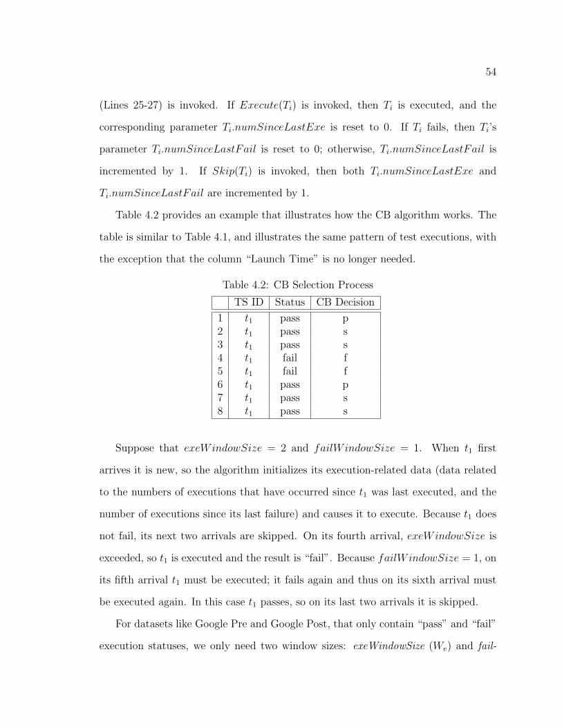
54
(Lines 25-27) is invoked. If Execute(Ti
) is invoked, then T
i
is executed, and the
corresponding parameter T
i
.numSinceLastExe is reset to 0. If Ti
fails, then T
i
’s
parameter T
i
.numSinceLastFail is reset to 0; otherwise, Ti
.numSinceLastFail is
incremented by 1. If Skip(Ti
) is invoked, then both T
i
.numSinceLastExe and
T
i
.numSinceLastFail are incremented by 1.
Table 4.2 provides an example that illustrates how the CB algorithm works. The
table is similar to Table 4.1, and illustrates the same pattern of test executions, with
the exception that the column “Launch Time” is no longer needed.
Table 4.2: CB Selection Process
TS ID Status CB Decision
1 t1 pass p2 t1 pass s3 t1 pass s4 t1 fail f5 t1 fail f6 t1 pass p7 t1 pass s8 t1 pass s
Suppose that exeWindowSize = 2 and failWindowSize = 1. When t1 first
arrives it is new, so the algorithm initializes its execution-related data (data related
to the numbers of executions that have occurred since t1 was last executed, and the
number of executions since its last failure) and causes it to execute. Because t1 does
not fail, its next two arrivals are skipped. On its fourth arrival, exeWindowSize is
exceeded, so t1 is executed and the result is “fail”. Because failWindowSize = 1, on
its fifth arrival t1 must be executed; it fails again and thus on its sixth arrival must
be executed again. In this case t1 passes, so on its last two arrivals it is skipped.
For datasets like Google Pre and Google Post, that only contain “pass” and “fail”
execution statuses, we only need two window sizes: exeWindowSize (We
) and fail-
55
WindowSize (Wf
) (as in Algorithm 2).
For datasets that contain more than just “pass” and “fail” execution statuses,
we need more parameters. As mentioned in Section 2.2.3.3, in addition to “pass”
and “fail”, the Rails dataset contains two more test suite result statuses: “error”
and “failerror”. In order to detect “error” and “failerror” statuses, we use exactly
the same method as to detect “fail” status. We add two more integer parameters,
errorWindowSize (Werr
) and failerrorWindowSize (Wfailerr
), corresponding to the
sizes of the error window and failerror window, and measured in terms of numbers of
test suites. Whenever a new test suite arrives, it will be assigned two more variables:
T
i
.numSinceLastError and T
i
.numSinceLastFailError. T
i
.numSinceLastError
records the number of times that T
i
has arrived but has been skipped or has not
encountered an “error” status since its last “error” status, and is initially set to 1.
T
i
.numSinceLastFailError records the number of times that Ti
has arrived but has
been skipped or has not encountered an “failerror” status since its last “failerror”
status, and is initially set to 1.
The selection process also has two more conditions: (1) if Ti
has been executed
and observed to encounter an “error” status within errorWindowSize times; and (2) if
T
i
has been executed and observed to encounter a “failerror” status within failerror-
WindowSize times. If any of the five conditions (these two additional conditions plus
the previous three) is satisfied, then T
i
should be executed, so Execute(Ti
) (Lines 17-
24) is invoked. If none of the five conditions are satisfied, then T
i
should be skipped,
so Skip(Ti
) (Lines 25-27) is invoked. In the Execute(Ti
) and Skip(Ti
) processes,
we also need to update T
i
.numSinceLastError and T
i
.numSinceLastFailError.
If Execute(Ti
) is invoked, then T
i
is executed, and the corresponding parameter
T
i
.numSinceLastExe is reset to 0. If Ti
fails, then T
i
’s parameter Ti
.numSinceLastFail
is reset to 0, but T
i
.numSinceLastError and T
i
.numSinceLastError are incre-
56
mented by 1; if Ti
occurs an “error” status, then T
i
.numSinceLastError is reset
to 0, but Ti
.numSinceLastFail and T
i
.numSinceLastFailError are incremented by
1; if Ti
occurs a “failerror” status, then T
i
.numSinceLastFailError is reset to 0, but
T
i
.numSinceLastFail and T
i
.numSinceLastError are incremented by 1; otherwise,
T
i
.numSinceLastFail, Ti
.numSinceLastError and T
i
.numSinceLastFailError are
incremented by 1. If Skip(Ti
) is invoked, then T
i
.numSinceLastExe, Ti
.numSinceLastFail,
T
i
.numSinceLastError and T
i
.numSinceLastFailError are incremented by 1.
To simplify the combinations of We
, Wf
, Werr
and W
failerr
, we assign the same
values to W
f
, Werr
and W
failerr
, which means that the three types of malfunctions
have the same window sizes.
4.2.2 Transition-Based RTS Approach
As noted in Section 4.1, a new “failure” (transition from “pass to fail”) could provide
more information about new changes in the codebase. If we are able to detect more
“pass to fail” transitions in test suites, we are able to provide more precise predictions
of transitions both from “pass to fail” and “fail” to “fail”. To address this issue, we
improve the CB technique by adding one more condition: whether the test suite’s
“pass to fail” transition ratio is greater than a random number.
Algorithm 3 presents the TrB algorithm. In this algorithm, there are four param-
eters: a test suite T
i
, two integer parameter (exeWindowSize and failWindowSize),
and a threshold (randomNumber), which is a randomly generated number and ranges
from 0 to 100. The first three parameters are the same as those in the CB algorithm
(Algorithm 2). The exeWindowSize and failWindowSize parameters correspond to
the sizes of the execution and failure windows, and are measured in terms of numbers
of test suites.
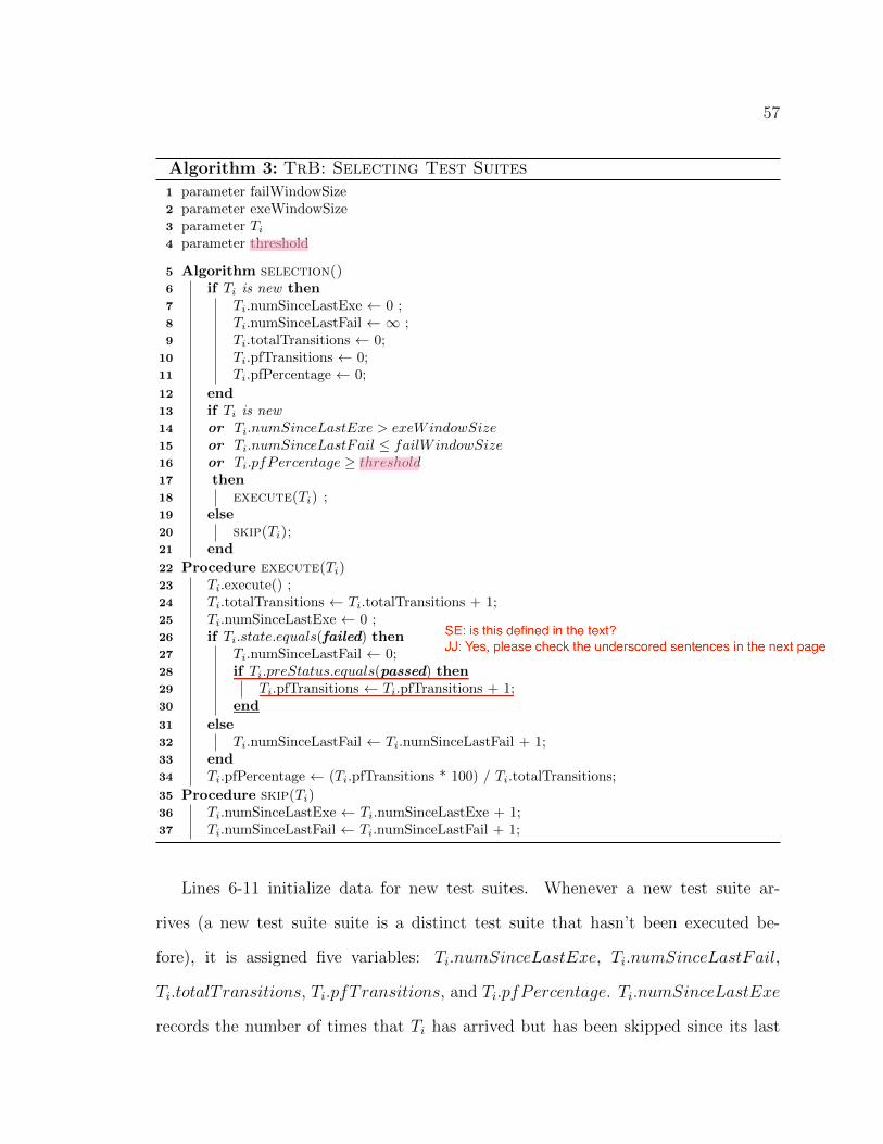
57
Algorithm 3: TrB: Selecting Test Suites
1 parameter failWindowSize2 parameter exeWindowSize3 parameter Ti
4 parameter threshold
5 Algorithm selection()
6 if Ti is new then
7 Ti.numSinceLastExe 0 ;8 Ti.numSinceLastFail 1 ;9 Ti.totalTransitions 0;
10 Ti.pfTransitions 0;11 Ti.pfPercentage 0;
12 end
13 if Ti is new
14 or Ti.numSinceLastExe > exeWindowSize
15 or Ti.numSinceLastFail failWindowSize
16 or Ti.pfPercentage � threshold
17 then
18 execute(Ti) ;
19 else
20 skip(Ti);
21 end
22 Procedure execute(Ti)
23 Ti.execute() ;24 Ti.totalTransitions Ti.totalTransitions + 1;25 Ti.numSinceLastExe 0 ;26 if Ti.state.equals(failed) then27 Ti.numSinceLastFail 0;28 if Ti.preStatus.equals(passed) then29 Ti.pfTransitions Ti.pfTransitions + 1;30 end
31 else
32 Ti.numSinceLastFail Ti.numSinceLastFail + 1;33 end
34 Ti.pfPercentage (Ti.pfTransitions * 100) / Ti.totalTransitions;
35 Procedure skip(Ti)
36 Ti.numSinceLastExe Ti.numSinceLastExe + 1;37 Ti.numSinceLastFail Ti.numSinceLastFail + 1;
Lines 6-11 initialize data for new test suites. Whenever a new test suite ar-
rives (a new test suite suite is a distinct test suite that hasn’t been executed be-
fore), it is assigned five variables: T
i
.numSinceLastExe, T
i
.numSinceLastFail,
T
i
.totalT ransitions, Ti
.pfTransitions, and T
i
.pfPercentage. Ti
.numSinceLastExe
records the number of times that T
i
has arrived but has been skipped since its last
58
execution, and is initially set to 0. Ti
.numSinceLastFail records the number of times
that T
i
has arrived but has been skipped or not failed since its last failure, and is
initially set to 1 . T
i
.totalT ransitions records the total transitions taken by T
i
.
T
i
.pfTransitions records the total number of “pass to fail” transitions, and is ini-
tially set to 0. Ti
.pfPercentage calculates the percentage of “pass to fail” transitions
over the total transitions of Ti
. For example, if Ti
has been executed 5 times with exe-
cution status: “pass”, “fail”, “fail”, “pass”, “fail”, then T
i
.totalT ransitions will be 5,
corresponding to the transitions: “new to pass”, “pass to fail”, “fail to fail”, “fail to
pass” and “pass to fail”. It is also initially set to 0. Ti
.pfTransitions will be 2, since
there are 2 “pass to fail” transitions among the 5 transitions. T
i
.pfPercentage will
be 60% which is calculated by (Ti
.pfTransitions * 100)/Ti
.totalT ransitions, and is
initially set to 0.
The selection process has four conditions (Lines 13-21): (1) if Ti
is new; (2) if Ti
has been skipped more than exeWindowSize times; (3) if Ti
has been executed and
observed to fail within the previous failWindowSize times; and (4) if Ti
’s “pass to
fail” transitions’ percentage is greater than or equal to the threshold (a random num-
ber). If any of these conditions is satisfied, then T
i
will be executed, so Execute(Ti
)
(Lines 22-34) is invoked. If none of these conditions are satisfied, then T
i
will be
skipped, so Skip(Ti
) (Lines 35-37) is invoked. If Execute(Ti
) is invoked, then T
i
will
be executed, Ti
.totalT ransitions will be incremented by 1, and the corresponding
parameter T
i
.numSinceLastExe will be reset to 0. If Ti
fails, then T
i
’s parameter
T
i
.numSinceLastFail is reset to 0; otherwise, Ti
.numSinceLastFail is incremented
by 1. In addition, in the case in which T
i
’s current execution status is “fail” (Line
26) and its previous execution status was “pass” (Line 28), indicating a“pass to fail”
transition, Ti
.pfTransitions is incremented by 1. Finally, Ti
.pfPercentage is calcu-
lated by ( Ti
.pfTransitions * 100)/Ti
.totalT ransitions. If Skip(Ti
) is invoked, then
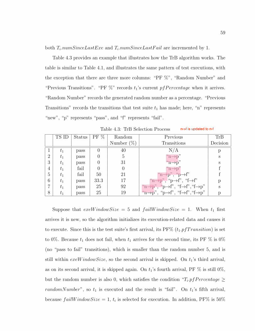
59
both T
i
.numSinceLastExe and T
i
.numSinceLastFail are incremented by 1.
Table 4.3 provides an example that illustrates how the TrB algorithm works. The
table is similar to Table 4.1, and illustrates the same pattern of test executions, with
the exception that there are three more columns: “PF %”, “Random Number” and
“Previous Transitions”. “PF %” records t1’s current pfPercentage when it arrives.
“Random Number” records the generated random number as a percentage. “Previous
Transitions” records the transitions that test suite t1 has made; here, “n” represents
“new”, “p” represents “pass”, and “f” represents “fail”.
Table 4.3: TrB Selection Process
TS ID Status PF % Random Previous TrBNumber (%) Transitions Decision
1 t1 pass 0 40 N/A p2 t1 pass 0 5 “n!p” s3 t1 pass 0 31 “n!p” s4 t1 fail 0 0 “n!p” f5 t1 fail 50 21 “n!p”, “p!f” f6 t1 pass 33.3 17 “n!p”, “p!f”, “f!f” p7 t1 pass 25 92 “n!p”, “p!f”, “f!f”,“f!p” s8 t1 pass 25 19 “n!p”, “p!f”, “f!f”,“f!p” p
Suppose that exeWindowSize = 5 and failWindowSize = 1. When t1 first
arrives it is new, so the algorithm initializes its execution-related data and causes it
to execute. Since this is the test suite’s first arrival, its PF% (t1.pfTransition) is set
to 0%. Because t1 does not fail, when t1 arrives for the second time, its PF % is 0%
(no “pass to fail” transitions), which is smaller than the random number 5, and is
still within exeWindowSize, so the second arrival is skipped. On t1’s third arrival,
as on its second arrival, it is skipped again. On t1’s fourth arrival, PF % is still 0%,
but the random number is also 0, which satisfies the condition “Ti
.pfPercentage �
randomNumber”, so t1 is executed and the result is “fail”. On t1’s fifth arrival,
because failWindowSize = 1, ti
is selected for execution. In addition, PF% is 50%
60
(currently, t1 has a “new to fail” and a“pass to fail” transition), and PF% is greater
than random number 21, so the fifth arrival satisfies two conditions. Test suite t1 fails
again and thus on its sixth arrival, it must be executed again because of its recently
failure. Since currently t1 has a “new to fail”, a“pass to fail”, and a “fail to fail”
transition, its PF% is updated to 33.3%. In this case t1 passes, and the PF% (25%)
is lower than random number 92%, so on its seventh arrival, it is skipped. On the
last arrival, t1 is executed because its PF% is 25, which is greater than the random
number 19%.
Similar to the Algorithm 2 for the CB technique, Algorithm 3 for the TrB tech-
nique provides a basic algorithm that only considers the case when the dataset
only contains “pass” and “fail” execution statuses. For the Rails dataset that con-
tains more malfunction types, we need more parameters. In order to detect “pass
to error” and “pass to failerror” transitions, we use exactly the same method as
to detect “pass to fail” transitions. We add two more integer parameters, error-
WindowSize (Werr
) and failerrorWindowSize (Wfailerr
), corresponding to the sizes
of the error window and failerror window, and measured in terms of numbers of
test suites. Whenever a new test suite arrives, it will be assigned more variables:
T
i
.numSinceLastError, Ti
.peTransitions, and T
i
.pePercentage for the “error” sta-
tus, and T
i
.numSinceLastFailError, Ti
.pfeTransitions, and T
i
.pfePercentage for the
“failerror” status. The selection process also has more conditions: (1) if Ti
has been
executed and observed to encounter an “error” status within errorWindowSize times;
(2) if Ti
has been executed and observed to encounter a “failerror” status within fail-
errorWindowSize times; (3) if Ti
’s “pass to error” transitions’ percentage is greater
than or equal to a random number; and (4) if Ti
’s “pass to failerror” transitions’
percentage is greater than or equal to a random number. All the variables’ updating
process and initial settings are exactly the same as those for the “fail” status.
61
To simplify the combinations of We
, Wf
, Werr
and W
failerr
, we assign the same
values to W
f
, Werr
and W
failerr
, which means that the three types of malfunctions
have the same window sizes.
4.3 Empirical Study
We wish to evaluate and compare the cost-e↵ectiveness of our two approaches, and
also to assess the e↵ects on cost-e↵ectiveness that result from the use of di↵erent
window sizes.
We conducted a study with the goal of investigating the following research ques-
tion:
RQ: How do our two RTS techniques perform in terms of malfunction detection
and “pass to malfunction” transition detection, and how do their malfunction de-
tection and transition detection vary with di↵erent settings of exeWindowSize (We
),
failWindowSize (Wf
), and where applicable, errorWindowSize (Werr
) and failerror-
WindowSize (Wfailerr
) on the Rails dataset?
4.3.1 Objects of Analysis
As with our CCBP technique, the objects of analysis we utilize are the CI data sets
described in Section 2: two from the Google Dataset and one from Rails.
4.3.2 Variables and Measures
4.3.2.1 Independent Variables
Our independent variables involve the techniques and windows used. We use the two
techniques presented in Section 4.2: CB and TrB.
62
For both the CB and TrB techniques, we utilize six values of failWindowSize (Wf
),
W
f
= {1, 2, 4, 5, 10, 100}.
To compare the performance of the two algorithms more fairly, we chose execution
window sizes that cause the CB and TrB algorithms to select approximately equal
percentages of test suites. This required us to select di↵erent exeWindowSize (We
)
values for the two algorithms. For the CB algorithm, the window sizes on Google
Post, Google Pre and Rails are W
e
= {1, 2, 4, 5, 10, 55}. For the TrB algorithm, the
window sizes on Google Post, Google Pre and Rails are W
e
= {1, 2, 4, 5, 10, 100}.
In addition to failWindowSize (Wf
) and exeWindowSize (We
), on the Rails dataset,
we also set errorWindowSize (Werr
) and failerrorWindowSize (Wfailerr
) for “error”
and “failerror” test suites to W
err
= {1, 2, 4, 5, 10, 100} and W
failerr
= {1, 2, 4, 5,
10, 100}.
4.3.2.2 Dependent Variables
As dependent variables we measure the percentage of failures detected, and the per-
centages of “pass to fail” transitions detected by our techniques, on Google Post and
Google Pre.
For Rails, we also measure the percentages of failures, errors, and failerrors de-
tected, and the percentages of “pass to fail”, “pass to error”, and “pass to failerror”
transitions.
We do the forgoing for each combination of We
and W
f
on all three datasets. To
simplify the combinations of pairs, Werr
and W
failerror
use the same value as W
f
.
Details are provided in Section 4.2.1 and Section 4.2.2.
63
4.3.3 Study Operation
On the GSDTSR and Rails datasets, we simulated a CI environment. We imple-
mented the CB and TrB techniques presented in Section 4.2, using approximately
400 lines of Java for each. Our simulation walks through the datasets, simulates their
execution, and records when malfunctions and transitions would be detected.
The CB technique utilizes failure and execution window sizes in terms of numbers
of test suites (parameters failWindowSize and exeWindowSize in Algorithm 2), and
reports the number of test suites selected, the number of failures/errors/failerrors
detected, and the transitions of “pass to fail” (“pass to fail”, “pass to error” and
“pass to failerror” on the Rails dataset) detected. It does this by reading each line
from the GSDTSR and Rails datasets, determining whether the test suite in the line
would be executed given the failure and execution windows, and updating the latest
failure and execution information for the test suite. If the test suite is to be executed,
then the implementation updates the test suite counter, the failure counter (if the test
suite resulted in a failure), the error counter and the failerror counter (if the dataset
is Rails and the test suite resulted in an error or a failerror). If the test suite’s
last execution status is “pass” and current execution status is “fail” (“error” and
“failerror” in Rails), then the implementation updates the corresponding transition
counter.
The same as the CB technique, the TrB technique utilizes failure and execution
window sizes in terms of numbers of test suites (parameters failWindowSize and ex-
eWindowSize in Algorithm 3) and the corresponding reporting process is also similar.
A key di↵erence is that the TrB technique utilizes one more parameter: a threshold
(a parameter threshold in Algorithm 3). In the simulation process, in addition to
the processes used for the CB technique, the TrB technique also records each test
64
suite’s percentage of “pass to fail” transitions (“pass to error” and “pass to failError”
transitions in Rails). When determining whether the test suite would be executed, in
addition to the failure and execution windows, it also checks whether the percentage
of “pass to fail” transitions (“pass to error” or “pass to failerror” transitions in Rails)
is greater than the threshold. If the transition percentage is greater than the random
number, then the test suite would be executed.
4.3.4 Threats to Validity
Where external validity is concerned, we have applied the CB and TrB techniques
to three extensive datasets; two of these are drawn from one large industrial setting
(Google) and the third from an open-source setting (Rails). The datasets have large
amounts and high rates of code churn, and reflect extensive testing processes, so our
findings may not extend to systems that evolve more slowly. We have compared
the two techniques, but we have not considered other alternative RTS techniques
(primarily because these would require substantial changes to work under the CI
settings we are operating in such as the random selection). We have utilized various
window sizes, but have necessarily limited our choices to a finite set of possible sizes.
We have not considered factors related to the availability of computing infrastructure,
such as variance in numbers of platforms available for use in testing. These threats
must be addressed through further study.
Where internal validity is concerned, malfunctions in the tools used to simulate
our RTS techniques on the datasets could cause problems in our results. To guard
against these, we carefully tested our tools against small portions of the datasets on
which results could be verified. Further, we have not considered possible variations
in testing results that may occur when test results are inconsistent (as might happen
in the presence of “flaky test suites”); such variations, if present in large numbers,
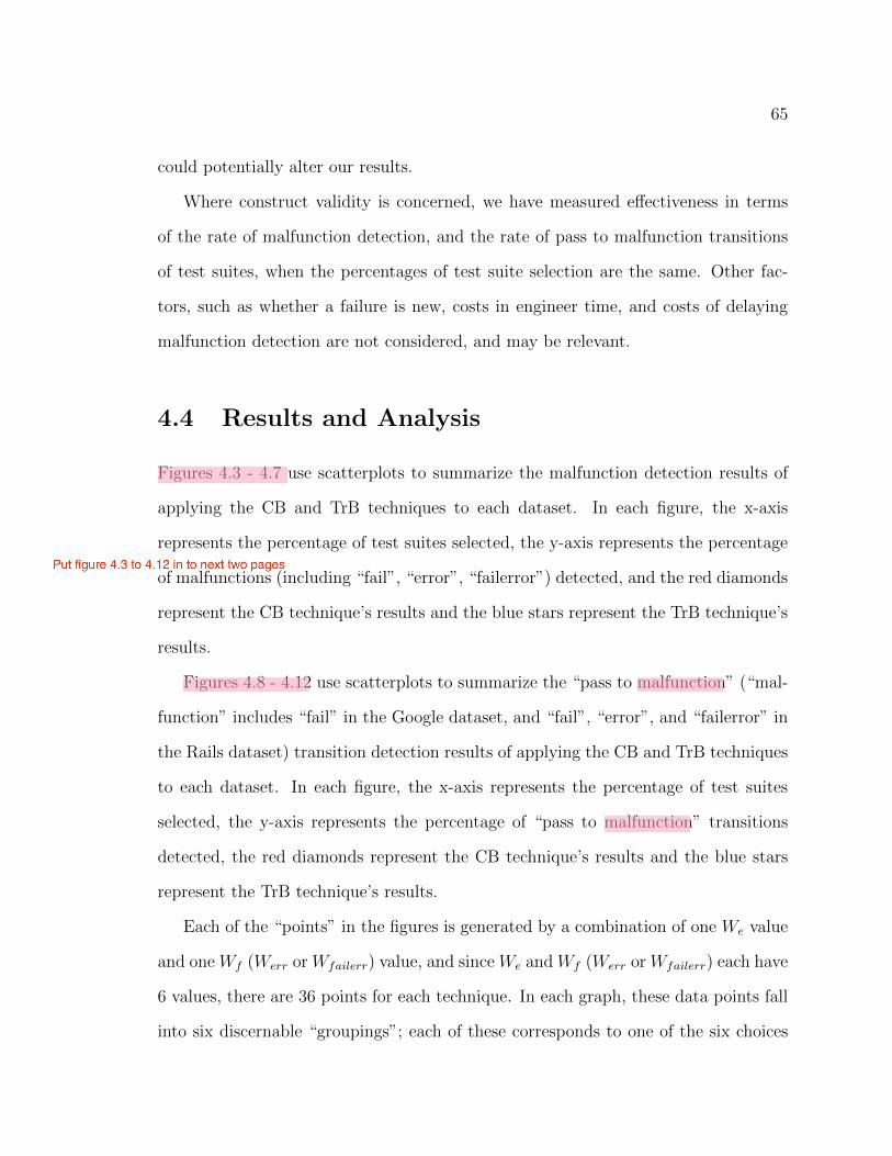
65
could potentially alter our results.
Where construct validity is concerned, we have measured e↵ectiveness in terms
of the rate of malfunction detection, and the rate of pass to malfunction transitions
of test suites, when the percentages of test suite selection are the same. Other fac-
tors, such as whether a failure is new, costs in engineer time, and costs of delaying
malfunction detection are not considered, and may be relevant.
4.4 Results and Analysis
Figures 4.3 - 4.7 use scatterplots to summarize the malfunction detection results of
applying the CB and TrB techniques to each dataset. In each figure, the x-axis
represents the percentage of test suites selected, the y-axis represents the percentage
of malfunctions (including “fail”, “error”, “failerror”) detected, and the red diamonds
represent the CB technique’s results and the blue stars represent the TrB technique’s
results.
Figures 4.8 - 4.12 use scatterplots to summarize the “pass to malfunction” (“mal-
function” includes “fail” in the Google dataset, and “fail”, “error”, and “failerror” in
the Rails dataset) transition detection results of applying the CB and TrB techniques
to each dataset. In each figure, the x-axis represents the percentage of test suites
selected, the y-axis represents the percentage of “pass to malfunction” transitions
detected, the red diamonds represent the CB technique’s results and the blue stars
represent the TrB technique’s results.
Each of the “points” in the figures is generated by a combination of one We
value
and oneWf
(Werr
orWfailerr
) value, and sinceWe
andW
f
(Werr
orWfailerr
) each have
6 values, there are 36 points for each technique. In each graph, these data points fall
into six discernable “groupings”; each of these corresponds to one of the six choices

66
0 20 40 60 80 100
020
4060
8010
0
% of Test Suites Selected
% o
f Fai
ling
Test
Sui
tes
Det
ecte
d
Result−Based RTS SelectionTransition−Based RTS Selection
Figure 4.3: Failure detection on Google-Post
0 20 40 60 80 100
020
4060
8010
0
% of Test Suites Selected
% o
f Fai
ling
Test
Sui
tes
Det
ecte
d
Result−Based RTS SelectionTransition−Based RTS Selection
Figure 4.4: Failure detection onGooglePre
0 20 40 60 80 100
020
4060
8010
0
% of Test Suites Selected
% o
f Fai
ling
Test
Sui
tes
Det
ecte
d
0 20 40 60 80 100
020
4060
8010
0
% of Test Suites Selected
% o
f Fai
ling
Test
Sui
tes
Det
ecte
d
Result−Based RTS SelectionTransition−Based RTS Selection
Figure 4.5: Failure detection on Rails
0 20 40 60 80 100
020
4060
8010
0
% of Test Suites Selected
% o
f Err
ored
Tes
t Sui
tes
Det
ecte
d
0 20 40 60 80 100
020
4060
8010
0
% of Test Suites Selected
% o
f Err
ored
Tes
t Sui
tes
Det
ecte
d
Result−Based RTS SelectionTransition−Based RTS Selection
Figure 4.6: Error detection on Rails
0 20 40 60 80 100
020
4060
8010
0
% of Test Suites Selected
% o
f Fai
lErr
ored
Tes
t Sui
tes
Det
ecte
d
0 20 40 60 80 100
020
4060
8010
0
% of Test Suites Selected
% o
f Fai
lErr
ored
Tes
t Sui
tes
Det
ecte
d
Result−Based RTS SelectionTransition−Based RTS Selection
Figure 4.7: FailError detection on Rails
0 20 40 60 80 100
020
4060
8010
0
% of Test Suites Selected
% o
f Pas
s to
Fai
l Tra
nsiti
ons
Det
ecte
d
Result−Based RTS SelectionTransition−Based RTS Selection
Figure 4.8: “Pass to Fail” transition de-tection on GooglePost
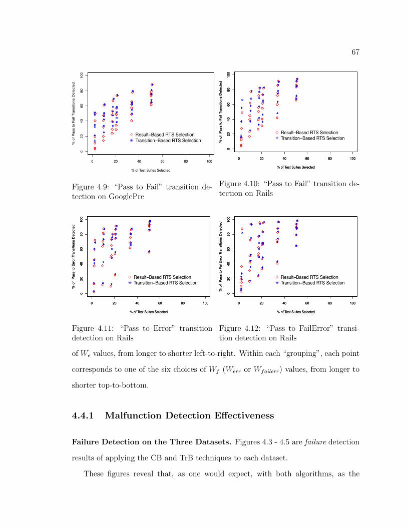
67
0 20 40 60 80 100
020
4060
8010
0
% of Test Suites Selected
% o
f Pas
s to
Fai
l Tra
nsiti
ons
Det
ecte
d
Result−Based RTS SelectionTransition−Based RTS Selection
Figure 4.9: “Pass to Fail” transition de-tection on GooglePre
0 20 40 60 80 100
020
4060
8010
0
% of Test Suites Selected
% o
f Pa
ss to
Fai
l Tra
nsiti
ons
Det
ecte
d
0 20 40 60 80 100
020
4060
8010
0
% of Test Suites Selected
% o
f Pa
ss to
Fai
l Tra
nsiti
ons
Det
ecte
d
Result−Based RTS SelectionTransition−Based RTS Selection
Figure 4.10: “Pass to Fail” transition de-tection on Rails
0 20 40 60 80 100
020
4060
8010
0
% of Test Suites Selected
% o
f Pa
ss to
Err
or T
rans
ition
s D
etec
ted
0 20 40 60 80 100
020
4060
8010
0
% of Test Suites Selected
% o
f Pa
ss to
Err
or T
rans
ition
s D
etec
ted
Result−Based RTS SelectionTransition−Based RTS Selection
Figure 4.11: “Pass to Error” transitiondetection on Rails
0 20 40 60 80 100
020
4060
8010
0
% of Test Suites Selected
% o
f Pa
ss to
Fai
lErr
or T
rans
ition
s D
etec
ted
0 20 40 60 80 100
020
4060
8010
0
% of Test Suites Selected
% o
f Pa
ss to
Fai
lErr
or T
rans
ition
s D
etec
ted
Result−Based RTS SelectionTransition−Based RTS Selection
Figure 4.12: “Pass to FailError” transi-tion detection on Rails
of We
values, from longer to shorter left-to-right. Within each “grouping”, each point
corresponds to one of the six choices of Wf
(Werr
or Wfailerr
) values, from longer to
shorter top-to-bottom.
4.4.1 Malfunction Detection E↵ectiveness
Failure Detection on the Three Datasets. Figures 4.3 - 4.5 are failure detection
results of applying the CB and TrB techniques to each dataset.
These figures reveal that, as one would expect, with both algorithms, as the
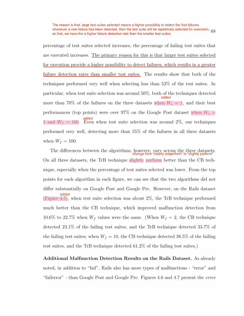
68
percentage of test suites selected increases, the percentage of failing test suites that
are executed increases. The primary reason for this is that larger test suites selected
for execution provide a higher possibility to detect failures, which results in a greater
failure detection rates than smaller test suites. The results show that both of the
techniques performed very well when selecting less than 52% of the test suites. In
particular, when test suite selection was around 50%, both of the techniques detected
more than 70% of the failures on the three datasets when W
e
= 1, and their best
performances (top points) were over 97% on the Google Post dataset when W
e
=
1 and W
f
= 100. Even when test suite selection was around 2%, our techniques
performed very well, detecting more than 55% of the failures in all three datasets
when W
f
= 100.
The di↵erences between the algorithms, however, vary across the three datasets.
On all three datasets, the TrB technique slightly perform better than the CB tech-
nique, especially when the percentage of test suites selected was lower. From the top
points for each algorithm in each figure, we can see that the two algorithms did not
di↵er substantially on Google Post and Google Pre. However, on the Rails dataset
(Figure 4.5), when test suite selection was about 2%, the TrB technique performed
much better than the CB technique, which improved malfunction detection from
10.6% to 22.7% when W
f
values were the same. (When W
f
= 2, the CB technique
detected 23.1% of the failing test suites, and the TrB technique detected 33.7% of
the failing test suites; when W
f
= 10, the CB technique detected 38.5% of the failing
test suites, and the TrB technique detected 61.2% of the failing test suites.)
Additional Malfunction Detection Results on the Rails Dataset. As already
noted, in addition to “fail”, Rails also has more types of malfunctions - “error” and
“failerror” - than Google Post and Google Pre. Figures 4.6 and 4.7 present the error
69
and failerror detection results from applying the CB and TrB techniques on the Rails
dataset.
Similar to failure detection trends, with both algorithms, as the percentage of test
suites selected increases, the percentage of executed test suites that display “error”
and “failerror” statuses increases. The results show that both of the techniques
performed well when selecting less than 52% of the test suites. In particular, when
test suite selection was around 50%, both of the techniques (on the Rails dataset)
detected more than 58% of errors and 74% of failerrors. The best performances (top
points) of both techniques detected more than 97% of errors and 98% of failerrors.
Even when test suite selection was around 2%, the techniques performed very well,
detecting more than 67% of errors and 80% of failerrors when W
err
= W
failerr
= 100.
Where these results di↵er from the failure detection on Rails is that, for both
error detection and failerror detection, even though the TrB technique still performed
better overall than the CB technique, the improvement was not substantial. By
comparing each pair of the algorithms’ data points generated byW
e
andW
err
/Wfailerr
combinations, most detection results from the TrB technique provided less than 8%
improvement over the CB technique.
In the failerror detection figure (Figure 4.7) when test suite selection was around
2%, the CB technique had several cases in which it performed better than the TrB
technique. One reason for this could be the di↵erence in W
e
value choices. In order
to select approximately equal percentages (2%) of the test suites, the W
e
value for
CB was 55, but the W
e
value for the TrB was 100. In this case, even though both
algorithms selected around 2% of the test suites, the results could be di↵erent. For
the CB technique with W
e
= 55, for each distinct test suite, if that test suite has
not yet detected a malfunction, it will be selected once for every other 55 arrivals.
However, for the TrB technique with W
e
= 100, for each distinct test suite, if that test
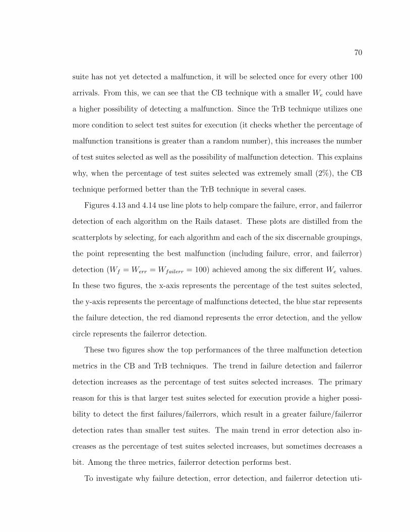
70
suite has not yet detected a malfunction, it will be selected once for every other 100
arrivals. From this, we can see that the CB technique with a smaller We
could have
a higher possibility of detecting a malfunction. Since the TrB technique utilizes one
more condition to select test suites for execution (it checks whether the percentage of
malfunction transitions is greater than a random number), this increases the number
of test suites selected as well as the possibility of malfunction detection. This explains
why, when the percentage of test suites selected was extremely small (2%), the CB
technique performed better than the TrB technique in several cases.
Figures 4.13 and 4.14 use line plots to help compare the failure, error, and failerror
detection of each algorithm on the Rails dataset. These plots are distilled from the
scatterplots by selecting, for each algorithm and each of the six discernable groupings,
the point representing the best malfunction (including failure, error, and failerror)
detection (Wf
= W
err
= W
failerr
= 100) achieved among the six di↵erent We
values.
In these two figures, the x-axis represents the percentage of the test suites selected,
the y-axis represents the percentage of malfunctions detected, the blue star represents
the failure detection, the red diamond represents the error detection, and the yellow
circle represents the failerror detection.
These two figures show the top performances of the three malfunction detection
metrics in the CB and TrB techniques. The trend in failure detection and failerror
detection increases as the percentage of test suites selected increases. The primary
reason for this is that larger test suites selected for execution provide a higher possi-
bility to detect the first failures/failerrors, which result in a greater failure/failerror
detection rates than smaller test suites. The main trend in error detection also in-
creases as the percentage of test suites selected increases, but sometimes decreases a
bit. Among the three metrics, failerror detection performs best.
To investigate why failure detection, error detection, and failerror detection uti-
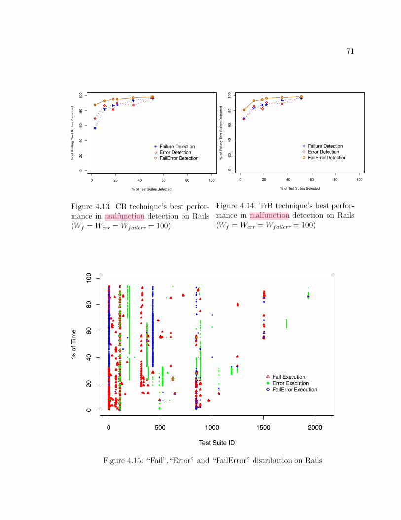
71
0 20 40 60 80 100
020
4060
8010
0
% of Test Suites Selected
% o
f Fai
ling
Test
Sui
tes
Det
ecte
d
●●●●
●
●
●
Failure DetectionError DetectionFailError Detection
Figure 4.13: CB technique’s best perfor-mance in malfunction detection on Rails(W
f
= W
err
= W
failerr
= 100)
0 20 40 60 80 100
020
4060
8010
0
% of Test Suites Selected
% o
f Fai
ling
Test
Sui
tes
Det
ecte
d
●●●●●
●
●
Failure DetectionError DetectionFailError Detection
Figure 4.14: TrB technique’s best perfor-mance in malfunction detection on Rails(W
f
= W
err
= W
failerr
= 100)
0 500 1000 1500 2000
020
4060
8010
0
Test Suite ID
% o
f Tim
e
Fail ExecutionError ExecutionFailError Execution
Figure 4.15: “Fail”,“Error” and “FailError” distribution on Rails
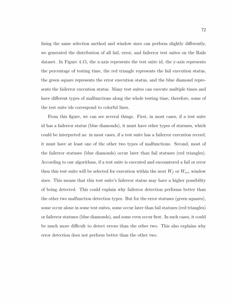
72
lizing the same selection method and window sizes can perform slightly di↵erently,
we generated the distribution of all fail, error, and failerror test suites on the Rails
dataset. In Figure 4.15, the x-axis represents the test suite id, the y-axis represents
the percentage of testing time, the red triangle represents the fail execution status,
the green square represents the error execution status, and the blue diamond repre-
sents the failerror execution status. Many test suites can execute multiple times and
have di↵erent types of malfunctions along the whole testing time, therefore, some of
the test suite ids correspond to colorful lines.
From this figure, we can see several things. First, in most cases, if a test suite
id has a failerror status (blue diamonds), it must have other types of statuses, which
could be interpreted as: in most cases, if a test suite has a failerror execution record,
it must have at least one of the other two types of malfunctions. Second, most of
the failerror statuses (blue diamonds) occur later than fail statuses (red triangles).
According to our algorithms, if a test suite is executed and encountered a fail or error
then this test suite will be selected for execution within the next Wf
or Werr
window
sizes. This means that this test suite’s failerror status may have a higher possibility
of being detected. This could explain why failerror detection performs better than
the other two malfunction detection types. But for the error statuses (green squares),
some occur alone in some test suites, some occur later than fail statuses (red triangles)
or failerror statuses (blue diamonds), and some even occur first. In such cases, it could
be much more di�cult to detect errors than the other two. This also explains why
error detection does not perform better than the other two.
73
4.4.2 Pass to Malfunction Transition Detection
E↵ectiveness
Pass to Fail Transition Detection on the Three Datasets. Figures 4.8 - 4.10
present the pass to fail transition detection results from applying the CB and TrB
techniques to each dataset.
These figures reveal that, with both algorithms, as the percentage of test suites
selected increases, the percentage of “pass to fail” transitions that are detected in-
creases. The primary reason for this is that larger test suites have a higher possibility
to detect the first “pass to fail” transitions, leading to repetitive selections of test
suites with higher “pass to fail” transition ratio, which result in a greater “pass to
fail” transition detection rates than smaller test suites. The results show that both
of the techniques performed very well when selecting less than 52% of test suites. In
particular, when test suite selection was around 50%, both techniques (on the three
datasets) detected more than 60% of the “pass to fail” transitions and their best per-
formances (top points) were over 94% on both the Google Post and Rails datasets.
Even when test suite selection was around 2%, our techniques performed very well,
detecting more than 49% of the failures in all three datasets when W
f
= 100.
The di↵erences between the algorithms, however, vary across the three datasets.
On all three datasets, the TrB technique slightly outperformed the CB technique,
especially when the percentage of test suites selected was lower. From the top points
for each algorithm in each figure, we can see that the two algorithms did not di↵er
substantially on Google Post and Google Pre. However, on the Rails dataset, when
test suite selection was about 2%, the TrB technique performed much better than the
CB technique, which improved the “pass to fail” transition detection from 11.9% to
27.9% when W
f
values were the same. (When W
f
= 1, the CB technique detected
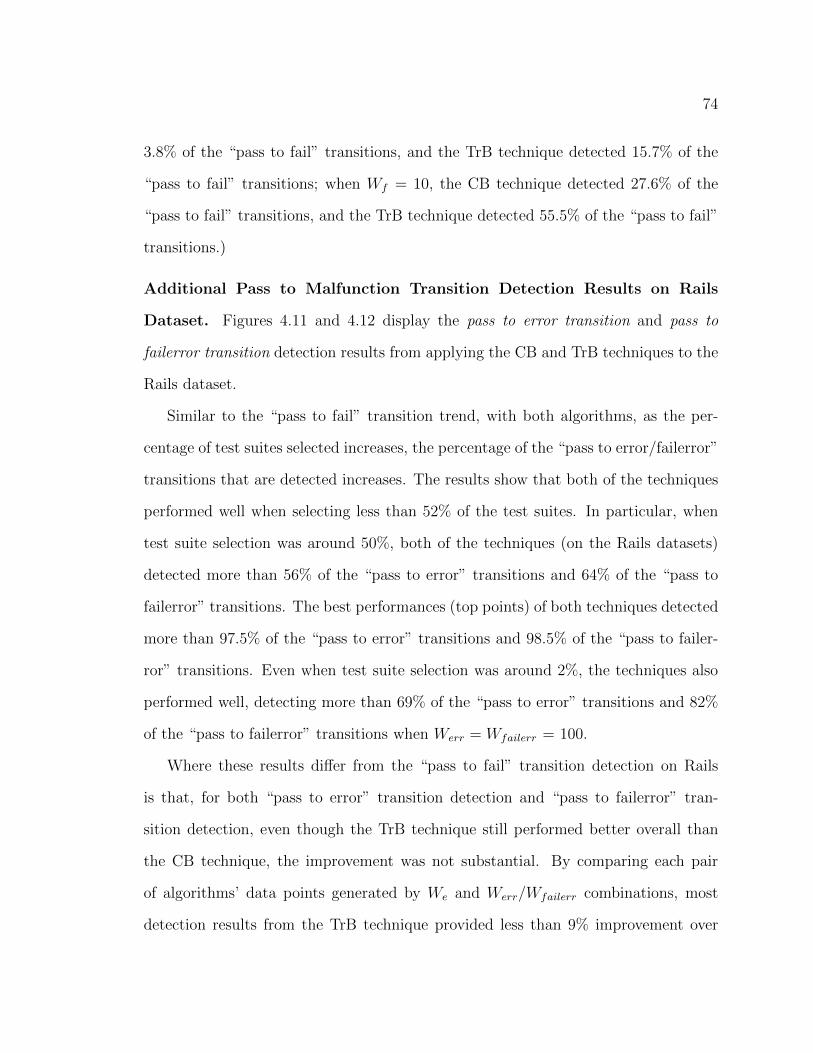
74
3.8% of the “pass to fail” transitions, and the TrB technique detected 15.7% of the
“pass to fail” transitions; when W
f
= 10, the CB technique detected 27.6% of the
“pass to fail” transitions, and the TrB technique detected 55.5% of the “pass to fail”
transitions.)
Additional Pass to Malfunction Transition Detection Results on Rails
Dataset. Figures 4.11 and 4.12 display the pass to error transition and pass to
failerror transition detection results from applying the CB and TrB techniques to the
Rails dataset.
Similar to the “pass to fail” transition trend, with both algorithms, as the per-
centage of test suites selected increases, the percentage of the “pass to error/failerror”
transitions that are detected increases. The results show that both of the techniques
performed well when selecting less than 52% of the test suites. In particular, when
test suite selection was around 50%, both of the techniques (on the Rails datasets)
detected more than 56% of the “pass to error” transitions and 64% of the “pass to
failerror” transitions. The best performances (top points) of both techniques detected
more than 97.5% of the “pass to error” transitions and 98.5% of the “pass to failer-
ror” transitions. Even when test suite selection was around 2%, the techniques also
performed well, detecting more than 69% of the “pass to error” transitions and 82%
of the “pass to failerror” transitions when W
err
= W
failerr
= 100.
Where these results di↵er from the “pass to fail” transition detection on Rails
is that, for both “pass to error” transition detection and “pass to failerror” tran-
sition detection, even though the TrB technique still performed better overall than
the CB technique, the improvement was not substantial. By comparing each pair
of algorithms’ data points generated by W
e
and W
err
/Wfailerr
combinations, most
detection results from the TrB technique provided less than 9% improvement over
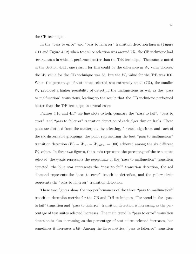
75
the CB technique.
In the “pass to error” and “pass to failerror” transition detection figures (Figure
4.11 and Figure 4.12) when test suite selection was around 2%, the CB technique had
several cases in which it performed better than the TrB technique. The same as noted
in the Section 4.4.1, one reason for this could be the di↵erence in W
e
value choices:
the W
e
value for the CB technique was 55, but the W
e
value for the TrB was 100.
When the percentage of test suites selected was extremely small (2%), the smaller
W
e
provided a higher possibility of detecting the malfunctions as well as the “pass
to malfunction” transitions, leading to the result that the CB technique performed
better than the TrB technique in several cases.
Figures 4.16 and 4.17 use line plots to help compare the “pass to fail”, “pass to
error”, and “pass to failerror” transition detection of each algorithm on Rails. These
plots are distilled from the scatterplots by selecting, for each algorithm and each of
the six discernable groupings, the point representing the best “pass to malfunction”
transition detection (Wf
= W
err
= W
failerr
= 100) achieved among the six di↵erent
W
e
values. In these two figures, the x-axis represents the percentage of the test suites
selected, the y-axis represents the percentage of the “pass to malfunction” transition
detected, the blue star represents the “pass to fail” transition detection, the red
diamond represents the “pass to error” transition detection, and the yellow circle
represents the “pass to failerror” transition detection.
These two figures show the top performances of the three “pass to malfunction”
transition detection metrics for the CB and TrB techniques. The trend in the “pass
to fail” transition and “pass to failerror” transition detection is increasing as the per-
centage of test suites selected increases. The main trend in “pass to error” transition
detection is also increasing as the percentage of test suites selected increases, but
sometimes it decreases a bit. Among the three metrics, “pass to failerror” transition
76
0 20 40 60 80 100
020
4060
8010
0
% of Test Suites Selected
% o
f Fai
ling
Test
Sui
tes
Det
ecte
d
●●●●
●
●
●
Pass to Fail Transition DetectionPass to Error Transition DetectionPass to FailError Transition Detection
Figure 4.16: CB technique’s best per-formance in Pass to Malfunction transi-tion detection on Rails (W
f
= W
err
=W
failerr
= 100)
0 20 40 60 80 100
020
4060
8010
0
% of Test Suites Selected
% o
f Fai
ling
Test
Sui
tes
Det
ecte
d
●●●
●●
●
●
Pass to Fail Transition DetectionPass to Error Transition DetectionPass to FailError Transition Detection
Figure 4.17: TrB technique’s best per-formance of Pass to Malfunction transi-tion detection on Rails (W
f
= W
err
=W
failerr
= 100)
detection performs best.
The reason “pass to fail” transition, “pass to error” transition and “pass to fail-
error” transition detection utilizing the same selection method and window sizes can
perform slightly di↵erently is similar to the three types of malfunction detection dif-
ferences (Section 4.4.1). Figure 4.15 shows some findings. First, in most cases, if a
test suite has a “failerror” execution record, it must have at least one of the other
two types of malfunctions. Second, most of the “failerror” execution records occur
later than the “fail” ones. According to our algorithms, if a test suite is executed
and encountered a “fail” or “error”, then this test suite will be selected for execution
within the next Wf
or Werr
window sizes. This means that this test suite’s “failerror”
status may have a higher possibility of being detected, which also indicates a higher
possibility of the “pass to failerror” transition detection. This could explain why
the “pass to failerror” transition detection performs better than the “pass to fail”
and “pass to error” transition detection types. But for the “error” statuses (green
squares), some occur alone in some test suites, some occur later than “fail” statuses
77
(red triangles) or “failerror” statuses (blue diamonds), and some even occur first. In
such cases, it could be much more di�cult to detect the errors than the in other two.
This also explains why “pass to error” transition detection does not perform better
than the other two.
4.4.3 The E↵ect of We
and W
f
(Werr
/Wfailerr
) Selection
Window sizes are the key parameters for both the CB and TrB algorithms.
Figures 4.18 and 4.19 use scatterplots to show the trends of the percentage of
test suite selection, the percentage of failure detection, and the percentage of “pass
to fail” transition detection when applying the TrB technique to the Google Post
dataset. In Figure 4.18 , the failWindowSize (Wf
) is fixed and assigned 100, and
W
e
={1, 2, 4, 5, 10, 100}. In Figure 4.19 , the exeWindowSize (We
) is fixed and assigned
1, and W
f
={1, 2, 4, 5, 10, 100}.
In the two figures, the x-axis represents the W
e
or Wf
size, the y-axis represents
the percentage of test suites selected (blue stars), failures detected (red diamonds)
and “pass to fail” transitions detected (yellow circles).
Because the e↵ect of Wf
, Werr
and W
failerr
are similar, and their values are the
same in our experiments, we only discuss the e↵ect of Wf
in detail. The e↵ect of We
and W
f
on the trends of the percentage of test suite selection, failure detection, and
“pass to fail” transition detection with the CB and TrB techniques are similar, as
well so we only use TrB’s results on Google Post as an example for illustration.
E↵ects on the Percentage of Test Suite Selection. The exeWindowSize (We
)
decides how often a test suite Ti
should be executed. LetWe
be x, without considering
other conditions, then each distinct test suite T
i
will be selected for execution once
every other x times. Suppose T1 has in total 100 arrivals, and W
e
is 4, then T1 would
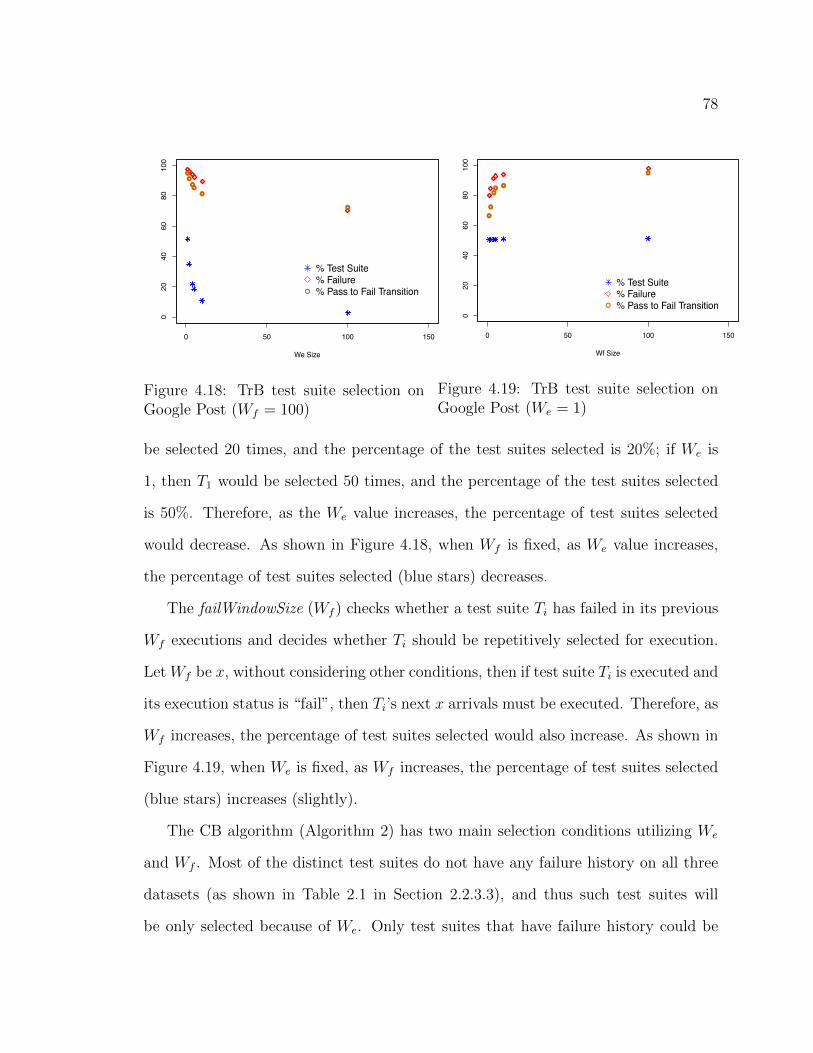
78
0 50 100 150
020
4060
8010
0
We Size
●●
●●
●
●
●
% Test Suite% Failure% Pass to Fail Transition
Figure 4.18: TrB test suite selection onGoogle Post (W
f
= 100)
0 50 100 150
020
4060
8010
0
Wf Size
●
●
●●
●
●
●
% Test Suite% Failure% Pass to Fail Transition
Figure 4.19: TrB test suite selection onGoogle Post (W
e
= 1)
be selected 20 times, and the percentage of the test suites selected is 20%; if We
is
1, then T1 would be selected 50 times, and the percentage of the test suites selected
is 50%. Therefore, as the W
e
value increases, the percentage of test suites selected
would decrease. As shown in Figure 4.18, when W
f
is fixed, as W
e
value increases,
the percentage of test suites selected (blue stars) decreases.
The failWindowSize (Wf
) checks whether a test suite T
i
has failed in its previous
W
f
executions and decides whether Ti
should be repetitively selected for execution.
LetWf
be x, without considering other conditions, then if test suite Ti
is executed and
its execution status is “fail”, then T
i
’s next x arrivals must be executed. Therefore, as
W
f
increases, the percentage of test suites selected would also increase. As shown in
Figure 4.19, when W
e
is fixed, as Wf
increases, the percentage of test suites selected
(blue stars) increases (slightly).
The CB algorithm (Algorithm 2) has two main selection conditions utilizing W
e
and W
f
. Most of the distinct test suites do not have any failure history on all three
datasets (as shown in Table 2.1 in Section 2.2.3.3), and thus such test suites will
be only selected because of We
. Only test suites that have failure history could be
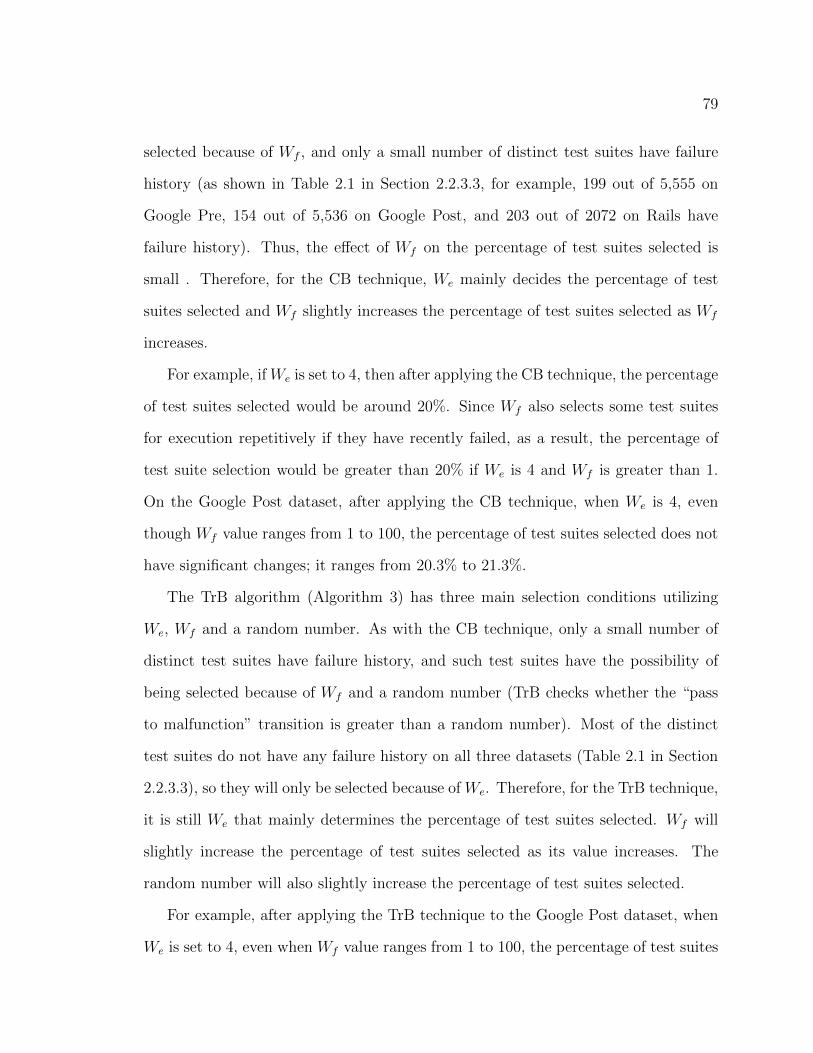
79
selected because of Wf
, and only a small number of distinct test suites have failure
history (as shown in Table 2.1 in Section 2.2.3.3, for example, 199 out of 5,555 on
Google Pre, 154 out of 5,536 on Google Post, and 203 out of 2072 on Rails have
failure history). Thus, the e↵ect of Wf
on the percentage of test suites selected is
small . Therefore, for the CB technique, We
mainly decides the percentage of test
suites selected and W
f
slightly increases the percentage of test suites selected as Wf
increases.
For example, ifWe
is set to 4, then after applying the CB technique, the percentage
of test suites selected would be around 20%. Since W
f
also selects some test suites
for execution repetitively if they have recently failed, as a result, the percentage of
test suite selection would be greater than 20% if We
is 4 and W
f
is greater than 1.
On the Google Post dataset, after applying the CB technique, when W
e
is 4, even
though W
f
value ranges from 1 to 100, the percentage of test suites selected does not
have significant changes; it ranges from 20.3% to 21.3%.
The TrB algorithm (Algorithm 3) has three main selection conditions utilizing
W
e
, Wf
and a random number. As with the CB technique, only a small number of
distinct test suites have failure history, and such test suites have the possibility of
being selected because of Wf
and a random number (TrB checks whether the “pass
to malfunction” transition is greater than a random number). Most of the distinct
test suites do not have any failure history on all three datasets (Table 2.1 in Section
2.2.3.3), so they will only be selected because ofWe
. Therefore, for the TrB technique,
it is still We
that mainly determines the percentage of test suites selected. W
f
will
slightly increase the percentage of test suites selected as its value increases. The
random number will also slightly increase the percentage of test suites selected.
For example, after applying the TrB technique to the Google Post dataset, when
W
e
is set to 4, even when W
f
value ranges from 1 to 100, the percentage of test suites
80
selected does not have significant changes; it ranges from 20.7% to 21.7%.
Compared with the CB technique, the TrB technique selects slightly more per-
centage of test suites when their W
e
and W
f
settings are the same. But when W
e
is large and the percentage of test suites selected is extremely small, then the dif-
ference matters. For example, on the Goole Post dataset, if W
e
= 100, and W
f
= {1, 2, 4, 5, 10, 100}, then CB’s percentage of test suites selected is {1.20%, 1.21%,
1.26%, 1.38%, 1.54%, 1.88%}. However, TrB’s percentage of test suites selected is
{2.03%, 2.07%, 2.19%, 2.26%, 2.28%, 2.74%}. To make the CB technique select an
approximately equal percentage of test suites as the TrB technique, we adjusted
W
e
to W
e
= {55} for CB; as a result, the corresponding selection percentage is
{2.04%, 2.05%, 2.12%, 2.25%, 2.36%, 2.78%}.
E↵ects on the Percentage of Malfunction Detection and Pass to Malfunc-
tion Transition Detection. As discussed in Sections 4.4.1 and 4.4.2, for both the
CB and TrB techniques, as the percentages of test suites selected increase, the corre-
sponding percentages of malfunction detection and “pass to malfunction” transition
detection also increase. The primary reason for this is that larger test suites tend to
have greater malfunction detection rates and “pass to malfunction” transition detec-
tion rates than smaller test suites. In addition, as in the previous section, we also
find that the percentage of test suites selected would decrease as W
e
increases, and
increase slightly as Wf
increases (on all three datasets).
From these two rules, we can see that as We
increases, the percentage of test suites
selected decreases, and thus the percentages of malfunction detection and “pass to
malfunction” transition detection also decrease. As Wf
increases, the percentage of
test suites selected increases, and thus the percentages of malfunction detection and
“pass to malfunction” transition detection also increase.
81
Figures 4.18 to 4.19 show examples of these trends. In Figure 4.18, Wf
is fixed,
and W
e
ranges from 1 to 100. As We
increases, the percentage of test suites selected
(blue stars) decreases, and the percentages of failure detection (red diamonds) and
“pass to fail” transition detection (yellow circles) also decrease. In Figure 4.19, We
is fixed, and W
f
ranges from 1 to 100. As Wf
value increases, the percentage of test
suites selected (blue stars) increases slightly, and the percentages of failure detection
(red diamonds) and “pass to fail” transition detection (yellow circles) increase rapidly
initially and level o↵ at around W
f
= 10.
The increasing rates of failure detection and “pass to fail” transition percentages
being higher than that of test suites selection percentage means that our W
f
(and
the random number in the TrB technique) contributes a lot to correctly predicting
the failures and “pass to fail” transitions.
4.5 Summary
We have presented two algorithms, the CB and TrB techniques, for improving the
cost-e↵ectiveness of RTS in CI environments. The CB technique utilizes two window
sizes in terms of numbers of test suites to select test suites based on failure and exe-
cution history. The TrB technique utilizes the test suites’ “pass to malfunction” tran-
sition history for selection in addition to the two windows used by the CB technique.
Compared with many prior techniques, both techniques use relatively lightweight
analysis, and do not require code instrumentation, rendering them appropriate for
CI environment testing. The empirical study results show that both algorithms can
detect malfunctions and “pass to malfunction” transitions cost-e↵ectively and on
comparison, the TrB technique performs slightly better for both of the metrics.
82
Chapter 5
Conclusions and Future Work
System builds and testing in CI environments are stunningly frequent, making it
important to address the costs of CI. To increase the rate of fault detection and reduce
the delays of testing feedback in CI environments, in this thesis, we have presented
a new TCP algorithm (the CCBP algorithm), and two new RTS algorithms (the CB
and TrB algorithms). The CCBP technique continuously prioritizes commits (not
test suites) as commits arrive or complete and our empirical results show that after
prioritization, our technique can e↵ectively detect failing commits earlier. The CB
technique selects test suites by using two window sizes in terms of numbers of test
suites based on failure and execution history. The TrB technique selects test suites
by using “pass to malfunction” transition history as well as the two windows. Our
empirical results show that after selection, both algorithms can detect malfunctions
and “pass to malfunction” transitions cost-e↵ectively, and the TrB technique performs
better than the CB technique.
CCBP, CB and TrB are lightweight approaches and operate quickly, allowing them
to be su�ciently responsive in CI environments. For the TCP technique, in future
work, we intend to further explore the e↵ects of factors such as the rate of change,
83
commit dependencies, and available resources, on the cost-e↵ectiveness of CCBP.
Given that results of the algorithm can vary with di↵erent workloads, we would like
to be able to dynamically adapt it to be more cost-e↵ective as workloads change.
This could apply, for example, when the computing resources available for testing
increase or decrease, or when arrival rates or sizes (in terms of associated test suites)
of commits change. For the RTS technique, in future work, we intend to explore
mechanisms for adjusting window sizes dynamically so that we can consider more of
the potential performance factors we have identified. Similarly, we would also like
to explore the e↵ects of history on the selection prediction so that we could consider
applying a “warm-up” period and a “moving history window” for collecting enough
recent history.
84
Bibliography
[1] S. Alspaugh, K.R. Walcott, M. Belanich, G.M. Kapfhammer, and M.L. So↵a.
E�cient time-aware prioritization with knapsack solvers. In Proceedings of the
ACM International Workshop on Empirical Assessment of Software Engineering
Languages and Technologies, pages 17–31, November 2007.
[2] J. Anderson, S. Salem, and H. Do. Improving the e↵ectiveness of test suite
through mining historical data. In Proceedings of the Working Conference on
Mining Software Repositories, pages 142–151, 2014.
[3] Atlassian. Atlassian software systems: Bamboo.
https://www.atlassian.com/software/bamboo, 2014.
[4] S. Bucur, V. Ureche, C. Zamfir, and G. Candea. Parallel symbolic execution for
automated real-world software testing. In Proceedings of the Sixth Conference
on Computer Systems, pages 183–198, 2011.
[5] Buildbot. https://buildbot.net, 2018.
[6] B. Busjaeger and T. Xie. Learning for test prioritization: An industrial case
study. In Proceedings of the International Symposium on Foundations of Software
Engineering, pages 975–980, 2016.
85
[7] A. Celik, A. Knaust, A. Milicevic, and M. Gligoric. Build system with lazy
retrieval for Java projects. In Proceedings of the International Symposium on
Foundations of Software Engineering, pages 643–654, 2016.
[8] H. Do, S. Mirarab, L. Tahvildari, and G. Rothermel. The e↵ects of time con-
straints on test case prioritization: A series of empirical studies. IEEE Transac-
tions on Software Engineering, 36(5), 2010.
[9] H. Do and G. Rothermel. On the use of mutation faults in empirical assessments
of test case prioritization techniques. IEEE Transactions on Software Engineer-
ing, 32(9), September 2006.
[10] E. D. Ekelund and E. Engstrom. E�cient regression testing based on test history:
An industrial evaluation. In International Conference on Software Maintenance
and Evolution, pages 449–457, September 2015.
[11] S. Elbaum, D. Gable, and G. Rothermel. The impact of software evolution
on code coverage. In Proceedings of the International Conference on Software
Maintenance, pages 169–179, November 2001.
[12] S. Elbaum, A. Malishevsky, and G. Rothermel. Incorporating varying test costs
and fault severities into test case prioritization. In Proceedings of the Interna-
tional Conference on Software Engineering, pages 329–338, 2001.
[13] S. Elbaum, A. G. Malishevsky, and G. Rothermel. Test case prioritization: A
family of empirical studies. IEEE Transactions on Software Engineering, 28(2),
2002.
[14] S. Elbaum, J. Penix, and A. McLaughlin. Google shared dataset of test suite
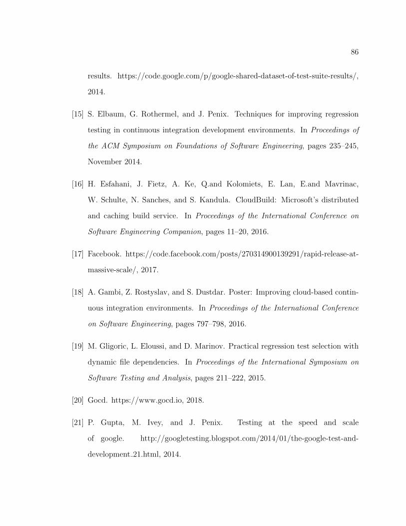
86
results. https://code.google.com/p/google-shared-dataset-of-test-suite-results/,
2014.
[15] S. Elbaum, G. Rothermel, and J. Penix. Techniques for improving regression
testing in continuous integration development environments. In Proceedings of
the ACM Symposium on Foundations of Software Engineering, pages 235–245,
November 2014.
[16] H. Esfahani, J. Fietz, A. Ke, Q.and Kolomiets, E. Lan, E.and Mavrinac,
W. Schulte, N. Sanches, and S. Kandula. CloudBuild: Microsoft’s distributed
and caching build service. In Proceedings of the International Conference on
Software Engineering Companion, pages 11–20, 2016.
[17] Facebook. https://code.facebook.com/posts/270314900139291/rapid-release-at-
massive-scale/, 2017.
[18] A. Gambi, Z. Rostyslav, and S. Dustdar. Poster: Improving cloud-based contin-
uous integration environments. In Proceedings of the International Conference
on Software Engineering, pages 797–798, 2016.
[19] M. Gligoric, L. Eloussi, and D. Marinov. Practical regression test selection with
dynamic file dependencies. In Proceedings of the International Symposium on
Software Testing and Analysis, pages 211–222, 2015.
[20] Gocd. https://www.gocd.io, 2018.
[21] P. Gupta, M. Ivey, and J. Penix. Testing at the speed and scale
of google. http://googletesting.blogspot.com/2014/01/the-google-test-and-
development 21.html, 2014.
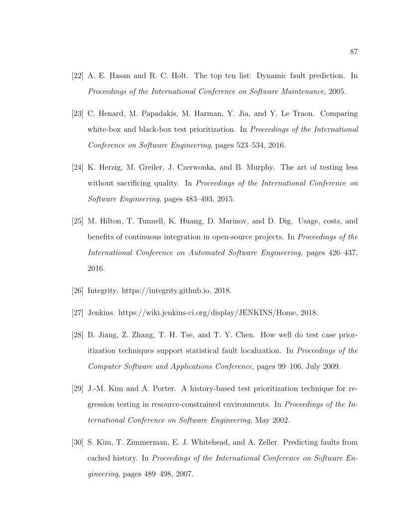
87
[22] A. E. Hasan and R. C. Holt. The top ten list: Dynamic fault prediction. In
Proceedings of the International Conference on Software Maintenance, 2005.
[23] C. Henard, M. Papadakis, M. Harman, Y. Jia, and Y. Le Traon. Comparing
white-box and black-box test prioritization. In Proceedings of the International
Conference on Software Engineering, pages 523–534, 2016.
[24] K. Herzig, M. Greiler, J. Czerwonka, and B. Murphy. The art of testing less
without sacrificing quality. In Proceedings of the International Conference on
Software Engineering, pages 483–493, 2015.
[25] M. Hilton, T. Tunnell, K. Huang, D. Marinov, and D. Dig. Usage, costs, and
benefits of continuous integration in open-source projects. In Proceedings of the
International Conference on Automated Software Engineering, pages 426–437,
2016.
[26] Integrity. https://integrity.github.io, 2018.
[27] Jenkins. https://wiki.jenkins-ci.org/display/JENKINS/Home, 2018.
[28] B. Jiang, Z. Zhang, T. H. Tse, and T. Y. Chen. How well do test case prior-
itization techniques support statistical fault localization. In Proceedings of the
Computer Software and Applications Conference, pages 99–106, July 2009.
[29] J.-M. Kim and A. Porter. A history-based test prioritization technique for re-
gression testing in resource-constrained environments. In Proceedings of the In-
ternational Conference on Software Engineering, May 2002.
[30] S. Kim, T. Zimmerman, E. J. Whitehead, and A. Zeller. Predicting faults from
cached history. In Proceedings of the International Conference on Software En-
gineering, pages 489–498, 2007.
88
[31] Y. Kim, M. Kim, and G. Rothermel. A scalable distributed concolic testing ap-
proach: An empirical evaluation. In Proceedings of the International Conference
on Software Testing, pages 340–349, April 2012.
[32] O. Legunsen, F. Hariri, A. Shi, Y. Lu, L. Zhang, and D. Marinov. An exten-
sive study of static regression test selection in modern software evolution. In
Proceedings of the International Symposium on Foundations of Software Engi-
neering, pages 583–594, 2016.
[33] J. Liang, S. Elbaum, and G. Rothermel. Continuous integration testing datasets.
https://github.com/elbaum/CI-Datasets, 2018.
[34] D. Marijan. Multi-perspective regression test prioritization for time-constrained
environments. In Proceedings of the IEEE International Conference on Software
Quality, Reliability and Security, pages 157–162, 2015.
[35] D. Marijan, A. Gotlieb, and S. Sen. Test case prioritization for continuous re-
gression testing: An industrial case study. In Proceedings of the International
Conference on Software Maintenance, pages 540–543, September 2013.
[36] A. Memon, Z. Gao, B. Nguyen, S. Dhanda, E. Nickell, R. Siemborski, and
J. Micco. Taming Google-scale continuous testing. In Proceedings of the Inter-
national Conference on Software Engineering: Software Engineering in Practice
Track, pages 233–242, 2017.
[37] Newrelic. https://blog.newrelic.com/2016/02/04/data-culture-survey-results-
faster-deployment/, 2016.
[38] J. Oqvist, G. Hedin, and B. Magnusson. Extraction-based regression test selec-
tion. In Proceedings of the International Conference on Principles and Practices
89
of Programming on the Java Platform: Virtual Machines, Languages, and Tools,
pages 5:1–5:10, 2016.
[39] A. Orso, N. Shi, and M. J. Harrold. Scaling regression testing to large soft-
ware systems. In Proceedings of the International Symposium on Foundations of
Software Engineering, pages 241–251, 2004.
[40] Rails. https://travis-ci.org/rails/rails, 2018.
[41] G. Rothermel and M. J. Harrold. A safe, e�cient regression test selection tech-
nique. ACM Transactions on Software Engineering and Methodology, 6(2):173–
210, 1997.
[42] G. Rothermel, R. Untch, C. Chu, and M. J. Harrold. Prioritizing test cases for
regression testing. IEEE Transactions on Software Engineering, 27(10):929–948,
2001.
[43] Gregg Rothermel and Mary Jean Harrold. Analyzing regression test selection
techniques. IEEE Transactions on Software Engineering, 22(8), August 1996.
[44] T. Savor, M. Douglas, M. Gentili, L. Williams, K. Beck, and M. Stumm. Contin-
uous Deployment at Facebook and OANDA. In Proceedings of the International
Conference on Software Engineering Companion, pages 21–30, 2016.
[45] A. Shi, S. Thummalapenta, S. K. Lahiri, N. Bjorner, and J. Czerwonka. Opti-
mizing test placement for module-level regression testing. In Proceedings of the
International Conference on Software Engineering, pages 689–699, 2017.
[46] A. Shi, T. Yung, A. Gyori, and D. Marinov. Comparing and combining test-
suite reduction and regression test selection. In Proceedings of the International
Symposium on Foundations of Software Engineering, pages 237–247, 2015.
90
[47] A. Srivastava and J. Thiagarajan. E↵ectively prioritizing tests in development
environment. In Proceedings of the ACM SIGSOFT International Symposium
on Software Testing and Analysis, 2002.
[48] M. Staats, P. Loyola, and G. Rothermel. Oracle-centric test case prioritization. In
Proceedings of the International Symposium on Software Reliability Engineering,
November 2012.
[49] Techbeacon. https://techbeacon.com/going-big-devops-how-scale-continuous-
delivery-success, 2016.
[50] ThoughtWorks. Go: Continous delivery. www.thoughtworks.com/products/go-
continuous-delivery, 2014.
[51] Travis ci. http://travis-ci.org, 2018.
[52] Travis ci api. https://travis-ci.com/api, 2018.
[53] A. Walcott, M.L. So↵a, G.M. Kapfhammer, and R.S. Roos. Time-aware test
suite prioritization. In Proceedings of the International Symposium on Software
Testing and Analysis, pages 1–12, July 2006.
[54] X. Wang and H. Zeng. History-based dynamic test case prioritization for re-
quirement properties in regression testing. In Proceedings of the International
Workshop on Continuous Software Evolution and Delivery, pages 41–47, 2016.
[55] L. White and B. Robinson. Industrial real-time regression testing and analy-
sis using firewalls. In Proceedings of the International Conference on Software
Maintenance, pages 18–27, September 2004.
[56] G. Wikstrand, R. Feldt, J. K. Gorantla, W. Zhe, and C. White. Dynamic regres-
sion test selection based on a file cache an industrial evaluation. In International
91
Conference on Software Testing Verification and Validation, pages 299–302, April
2009.
[57] S. Yoo, M. Harman, P. Tonella, and A. Susi. Clustering test cases to achieve
e↵ective and scalable prioritisation incorporating expert knowledge. In Proceed-
ings of the International Symposium on Software Testing and Analysis, pages
201–212, 2009.
[58] S. Yoo, R. Nilsson, and M. Harman. Faster fault finding at Google using multi
objective regression test optimisation. In Proceedings of the International Sympo-
sium on Foundations of Software Engineering, Industry Track, September 2011.
[59] L. Zhang, C. Hou, S.-S.and Guo, T. Xie, and H. Mei. Time-aware test-case pri-
oritization using integer linear programming. In Proceedings of the International
Symposium on Software Testing and Analysis, pages 213–224, July 2009.