1:XILINX

~--

Application Note

Counter Examples

l:XILINX

Introduction

Binary Counters

Johnson Counters

Linear feedback Shift Register Counters

Up/Down Counters . .

Heterodyne Counters

Counter Examples

Table of Contents

2-98

2-99

2-100

2-107

2-114

2-117

2-119

l:XILINX

INTRODUCTION

Historically, designers used multiple 74-series TTL devices to implement various digital counters. However, in application specific intergrated circuit (ASIC) designs the overall performance and effective utilization of a counter depends on the type of counter used and upon the architecture of the ASIC device employed. The flexible array architecture found in the Xilinx Logic Cell™ Array (LCA) provides the designer with numerous options when implementing counters. Implementing a design on "uncommitted" silicon is different from being forced into an inflexible, fixed architecture. Accordingly, a designer can optimize a counter to meet his specific application needs. Tailoring a counter for an application reduces the amount of wasted silicon resources associated with fixed-architecture logic devices.

Within a Logic Cell Array, a designer can implement various counter types, including

• Binary counters (2n possible states)

• Johnson counters (2n possible states)

• Linear Feedback Shift Registers (2n-1 possible states)

• Up/Down counters (typically binary)

• Heterodyne (mixed modulo)

tilillilliliiiii!i~~~l~iiilili By selecting the proper type of counter or even the right mix of counters, a designer maximizes performance and utilization within an LCA design. Choosing the right counter for the application depends on whether the counter application requires

• Binary or non-binary counting sequence, or

• High or low counter modulo, or

• Optimal performance, or • Optimal register and routing resource efficiency.

Some counter applications require control signals which

Counter Examples

may include parallel load of data, clock enable, synchronous or asynchronous SET or RESET, UP/DOWN control, or others. Synchronous binary counters are widely-used in digital design but their complexity can degrade their overall speed and effectiveness. The extra routing and logic required to implement a wide toggle lookahead-carry function, for example, quickly consumes the resources available in any logic device (a toggle lookahead-carry should not be confused with the lookahead-carry used in arithmetic logic). For speed, ease of routing, and glitch-free decoding, Johnson counters are often the best solution for applications of modulo ten or less. If a non-binary, pseudorandom counting sequence is acceptable, Linear Feedback Shift Register (LFSR) counters can best implement counts above modulo 32.

The purpose of this application note is to help the designer choose which counter to use for specific applications in the XC2064 and XC2018 Logic Cell Arrays (LCAs). Another goal is to help the designer start thinking about alternatives to 7400-series counters. There are various means of attacking the same counter application. A designer should use a specific type of counter to fill a specific application-not because it is the only counter type available but because it is the best counter for the specific application. The LCA gives the designer added flexibility, and this application note suggest ways to take advantage of this flexibility in counter designs. Descriptions of various counter applications are provided with examples wherever possible.

Resource Efficiency

Binary counters are more register efficient than other counter types since their capability increases as the exponent of the number of registers, as shown in Figure 1. Binary counters have up to 2n possible states. Sometimes, however, the more complex routing of a binary counter can make it less silicon efficient than a comparable counter of a different type. With only one less state than a binary counter of comparable size (2n-1), Linear Feedback Shift Registers follow closely behind in counting capability. The ease of routing within an LFSR counter design sometimes outweighs their non-binary, pseudorandom counting sequence. Lowest on the list of register efficiency is the Johnson or Mobius counter. With only 2n possible states, Johnson

2-99

Counter Examples

counters are less resource-efficient for modulos much higher than 12 (six registers). However, extremely high­performance Johnson counters can operate at speeds near the overall toggle frequency of the LCA since the counter logic and routing is simple.

Since each Configurable Logic Block (CLB) within the XC2064 and XC2018 Logic Cell Arrays has a single flip­flop or storage element, there is a direct relation between flip-flop efficiency and CLB efficiency. These terms are practically synonymous when referring to the counter bits required to implement a counter. Since some designs require additional logic beyond the logic associated with the flip-flop inside a CLB, some forms of counters require more CLBs than flip-flops.

BINARY COUNTERS

Overview

This section addresses the design and associated topics regarding binary ripple, ripple-carry, and lookahead-carry counters. The performance of a binary counter increases with the amount of lookahead-carry

220

218

216

performed at each counter stage. Simple ripple counters have no lookahead-carry and are the lowest­perfomance binary counter. Higher-performance binary counters require additional silicon resources to decode and propagate the carry signals. The ripple-carry and lookahead-carry counters require partial or full decoding of all of the previous counter bits. This requires extra logic and routing resources for the carry signals but buys increased performance.

Binary counters operate differently depending on the amount of lookahead carry. Simple ripple counters operate asynchronously since they do not generate carry signals, whereas ripple-carry and lookahead-carry counters are synchronous. Typically synchronous design is safer since it is more immune to glitches.

Ripple Counters

In simple binary ripple counters, as shown in Figure 2, carry signals are not generated. The output of each counter stage asynchronously clocks the next counter stage. The resource requirements to implement a ripple counter are low-only one CLB per counter bit regardless of counter length. The routing for a binary

'" '" " '"

'" '"

'/

" "

BINARYCOUNTERS ",'" 2N STATES (EXPONENTIAL) '" 214

212

COUNTER 2

10 MODULO

28

26

24

22

20

0 5

\ ",""

",'" LINEAR FEEDBACK '" SHIFT REGISTERS

1024 '" '" 2N_1 STATES (EXPONENTIAL)

JOHNSON COUNTERS 2N STATES (LINEAR)

20

10 15

COUNTER REGISTERS

20

0010023 1

Figure 1. Different types of counters require different amounts of registers and resources for the same task. The capability of binary counters increases exponentially with the number of bits while Johnson counters increase only linearly.

2-100

ripple counter is also simple. The penalty for this simplicity is lower performance. Each counter bit degrades the overall performance by a CLB delay time. The overall counter clock period must be greater than or equal to the total delay of all the CLBs used to implement the counter, as shown in Equation 1.

Ripple Counter = N • (Clock to Output Delay [1J Clock Period

where

N Clock to Output

0010023 2

= number of ripple counter flip-flops = Tcko for K-clock input = Tcco for C-clock input = Tcio for logic clock input

CLOCKH

RESETDIR

E:XILINX

Binary ripple counters are primarily used only in applications that require optimal device utilization without regard to performance. The increased silicon utilization is gained by eliminating carry signals. However, the flip-flops within a binary ripple counter are asynchronously toggled in operation. There are synchronous forms of this counter that have better performance and require the same resources. This is true because of the flexible array-type architecture of the LCA and because of the capability of a single CLB. An example is shown in Figure 3. This synchronous binary ripple-carry counter still requires only one CLB per bit. Since the ripple-carry includes only the previous counter stage, resource requirements are minimal. Its synchronous design affords more reliable operation.

Figure 2. Binary ripple counters are simple to implement and can be cascaded to nearly any desired length. Their disadvantage stems from their asynchronous operation and their degraded performance with each additional counter bit. They are not recommended for most designs because of their asynchronous operation.

0010023 3

TERMINAL COUNT

Figure 3. A single-bit ripple-carry counter requires as few resources as a standard ripple counter but has. synchronous operation. While highly CLB efficient, this design does have performance below counters with greater amounts of ripple-carry and below alilookahead-carry counters.

2-101

Counter Examples

Although the single-bit ripple-carry counter requires few resources, it still suffers from lower performance, much like the standard ripple counter. It also exhibits lower peformance with each additional CLB or flip-flop.

Ripple-Carry Counters

The design shown in Figure 3 is just one example of a binary ripple-carry counter. Ripple-counters have been used by designers for quite some time. In the past, designers typically implemented large binary ripple-carry counters with conventional 74-series logic devices. Designers tended to cascade the ripple-carry output of one 4-bit counter segment with the enable of the next 4-bit counter segment to build larger counters. Counter implementations within an LCA do not lend themselves to the "one size fits all" approach of the 74-series devices, since the architectures are different. However, some of the general ideas still apply.

Table 1 shows the wide variety of possible binary ripple­carry counters to eight bits in length. Larger ripple-carry counters are possible but there are far too many permutations to mention them all. The counters shown in the table consist of smaller counter segments, each with its own terminal count and clock enable. Larger counters can be built by cascading these segments together. The terminal count of one segment feeds the clock enable of the next segment and so on. The cascaded connection of the terminal count to clock enable is called a ripple-carry.

By cascading various counter segment macros together in the proper order, a designer can construct counters with various performances and control inputs. The table indicates the counter size in bits and in total modulo. The table also indicates whether CLOCK ENABLE (CE) or TERMINAL COUNT (TC) is available for that particular counter. The number of CLB logiC levels required to implement the counter function is displayed under "Ripple Levels". The higher the number of ripple levels, the slower the counter will run since each ripple level corresponds to a single CLB block delay.

The actual number of CLBs needed to implement a counter function depends on the number of control signals required. Wheras a simple CLOCK ENA.BLE (CE) and RESET take minimal resources, a PARALLEL ENABLE (PARENA) typically requires an additional CLB as shown in the table.

DESIGN EXAMPLE 1. Escaping from the TTL "one size fits all" approach. Building an eight-bit ripple-carry counter with 74-series TIL and with an LCA.

Assume that a counter application requires an eight-bit binary counter with reset. Figure 4a shows a common implementation of an eight-bit counter using two 74-161

TTL devices. A designer unfamiliar with the capability of the LCA might choose a similar implementation using two of the 74-161 counter macros available within the XAClTM Development System. However, a direct one­for-one substitution is wasteful. It would require sixteen CLBs to implement the two 74-161 equivalent circuits.

The Xilinx 74-161 macro contains the same functionality as a 74-161 device. Typically however, not all of the resources of a 74-161 are used in a design. This is the case in Figure 4a. Some of the CLB capability has been wasted on circuitry which will not be used for the design (Note: The Xilinx FutureNet Schematic Capture Library and Conversion Package reduces the macros to their primitive gate levels and then frees any unused resources).

A more rational approach uses only the required amount of circuitry to implement the design. For example, it is simpler and more resource efficient to build the eight-bit counter with the generic counter macros available within XACT. Table 1 shows some of the possible macro combinations used to build an eight-bit counter.

An equivalent counter built with two CBBC-rd counter macros and one C4BC-rd counter macro is shown in Figure 4b. The eight-bit counter is built with two 3-bit pieces and a single 2-bit piece. This implementation was chosen over using two 4-bit pieces since the former has superior performance. The 4-bit pieces each have two ripple-carry levels each. Therefore the eight-bit counter implemented with 4-bit pieces will have four ripple-carry delay levels overall. A similar implementation based on the two 3-bit pieces, and a 2-bit piece only has three ripple-carry delay levels, and therefore has higher performance.

Building the a-bit counter by cascading smaller counter macros reduces the number of required CLBs from sixteen to ten while simultaneously increasing performance.

Generally large ripple-carry counters should be built with multiple 3-bit pieces instead of 4-bit pieces since there are fewer ripple-carry delays through a 3-bit piece. The various ripple-carry possibilities are described in Table 1. When given a schematic drawn with 74-series devices, a designer should consider the function required for the application, and not blindly implement a one-for-one 74-series logic substitution.

DESIGN EXAMPLE 2. asynchronous design!

Avoiding the pitfalls of

A common practice when designing with 74-series devices is to use the terminal count of a counter as an asynchronous Signal to either RESET the counter or to load the counter with a predetermined value. Figure Sa

2-102

CI)

o a: () « ::E a: ~ z :::> o ()

b ~ x z ::J X

COUNTER SIZE AVAILABLE RIPPLE SELECTIONS LEVELS

2° 21 1 22 23 24 25 26 1 271 (Modulo) CE TC

8 (4) X X 1

FT C4B - X 1

C4B 1FT (8)

X - 1

C8B X X 1

FT C4B FT - - 1

FT C8B - X 1

C8B FT (16)

X - 1

C4B 1

C4B X X 2

FT C8B FT - - 1

FT C4B C4B - X 2

I (32)

C4B C4B FT X - 2

C8B C4B X X 2

FT C4B C4B FT - - 2

FT C8B C4B - X 2

C8B C4B FT (64) X - 2

C8B caB X X 2

C4B I C4B C4B X X 3

FT C8B C4B FT - - 2

FT caB C8B - X 2

FT C4B C4B C4B - X 3

C8B caB FT (128)

X - 2

C4B I C4B C4B FT X - 3

caB C4B C4B X X 3

FT C8B caB FT - - 2

FT C4B C4B 1 C4B FT - - 3

FT caB C4B C4B - X 3

C8B C4B I C4B FT (256)

X 3 -C8B caB C4B X X 4

C4B 1 C4B C4B C4B X X 4

NOTE: THE ABOVE COMBINATIONS MAY BE CASCADED FOR LARGER MODULO. CE/CLKENA = CLOCK ENABLE PARENA = PARALLEL ENABLE FT = TOGGLE FLIP-FLOP TC= TERMINAL COUNT

CLKENAOR CE&RESET

CLBs

3

3

4

4

4

5

5

4

6

5

5

6

6

7

7

a

6

8

9

7

9

7

a

10

a

9

9

10

a

Table 1. Binary ripple-carry counters from two to eight bits.

2-103

t:XILINX

CLKENA &PARENA

CLBs

3

4

4

5

5

6

6

6

7

7

7

8

8

9

9

10

9

10

11

10

11

10

11

12

11

12

12

13

12

I\) I .....

o ~

0010023 4A

CLKENA

CLOCK

RESETDIR

0010023 4B

+5

ENABLE

CLOCK

CLEAR

l 4

1

00-03

LO

CET 74-161

CEP

C

MR

+5V

TC 1 4 04-07

LO

~ ~ 74-161 ~ CEP

16CLBs

C

I MR

4

00--03 04-07

Figure 4a. An eight-bit counter with reset built with two 74-161 TTL devices. Notice that not all of the device connections are used to implement the function required. A direct 74-series SUbstitution proves wasteful. Use only the logic required to implement the required function.

L ______________________________________________________________ J __________________________________________________________________________________________________ --------

MACROC8BC-RD MACROC8BC-RD MACROC4BC-RD

Figure 4b. A better implementation of an eight-bit ripple-carry counter based on various macros from the XACT Development System. When designing with an LCA, an engineer can tailor his logic so that the LCA performs the required function with the minimum amount of logic.

g c: ::J -CD ... ~ I» 3 "0 (j) I/J

N , ..... o U1

0010023 5A

CLOCK

0010023 58

CLOCKH ~

RESETDIR a( RESET

Figure Sa. The asynchronous design practices of 74-series TTL devices are discouraged. An asynchronous design is less reliable and riskier since it is unforgiving to unknown design conditions.

0 0 0

R R R

Figure 5b. Synchronous design provides more relable operation.

RESET

M ~ C z ><

Counter Examples

demonstrates how a similar design might be implemented within an LCA although the asynchronous implementation is not recommended. The drawback to this design is that it is potentially unreliable. The terminal count (and RESET signal) is generated by ANDing all of the register outputs. When the counter reaches state 1111, the asynchronous RESET signal is asserted. Not all of the registers will be reset simultaneously because of the delay along the RESET network. Since the RESET signal is formed by the AND of the register outputs, the RESET signal will no longer be asserted and the remaining registers may fail to reset if anyone of the registers is reset before the others.

The asynchronous RESET signal will also experience decoding glitches as the various counter bits propagate through their nets to the AND gate. Any glitch on this signal can partially reset the counter.

An improved design appears in Figure 5b. In this example the RESET signal is asserted synchronously. This gives the synchronous RESET signal until the next clock edge to propagate to all of the CLBs and also prevents any of the CLBs from being reset by glitches on the RESET line. Since both asynchronous and synchronous RESET require a single CLB input, no more resources are required to build a completely syn?hronous design than the more risky asynchronous design. In general, synchronous design practices apply not only to counter design, but to all digital designs.

Lookahead-Carry Counters

There are applications where binary ripple and ripple­carry counters are too slow. In such cases, synchronous binary counters with lookahead-carry are an answer. Building high-performance synchronous binary ~ounters within an LCA is a simple process but, it Involves a few special techniques.

High-performance synchronous counters derive their speed by decoding lookahead-carry signals from all of the previ?us cou~ter stages. There is not a ripple-carry as descnbed earlier-ali of the previous counter outputs are decoded to form a single lookahead-carry signal for each counter stage. Combining all of the ripple-carry into a single lookahead-carry reduces overall design delays and increases performance.

Decoding lookahead-carry signals requires additional Configurable Logic Blocks (CLBs) in addition to more routing resources. The additional CLBs allow faster counters to be built. Higher performance is obtained by increasing the number of CLBs required to perform the function (divide and conquer!).

The generalized equation for synchronous binary lookahead-carry counters is given in Equation 2.

00 = ((CE • RESET· PARENA) EB 00) [2] +PARENA' DO

=-c-=-=~

01 = ((CE • RESET· PARENA • 00) EB 01) + PARENA * D1

On = ((CE' RESET· PARENA· 00 • 01 •...• On-1) EB On) + PARENA * Dn

where

CE RESET PARENA On Dn

= Clock Enable = Register Reset = Parallel Enable = Register Value = Register Input Value

Th~ .complexity of the counter can be reduced by omitting one or more of the control signals (Le., CE, RESET, etc.). For example, one way to remove RESET is to realize that all of the registers in the LCA are reset after configuration or any time the device RESET line has beerfasserted LOW.

From the generalized equation shown above, the overall complexity of the design grows with each additional counter bit. Since the CLBs within the XC2064 and XC2018 have up to four and sometimes five inputs, the logic equations for the counter bits need to be partitioned i~t.o s.maller pieces. Design Example 3 descnbes the partitioning of a 10-bit counter.

DESIGN EXAMPLE 3. A 10-bit synchronous binary counter with CLOCK ENABLE (CE) and RESET_DIRECT (RESET)

The 10-bit binary counter requires 14 Configurable Logic Blocks (CLBs)-ten blocks to implement the ten counter registers plus four additional blocks to generate the lookahead-carry logic. The clock signal (CLOCK) connects to the global clock buffer (upper left-hand corner of the die) to minimize clocking skew to each of the ~unter registers. The RESET_DIRECT signal feeds Into the reset-direct input to the flip-flop in each CLB (the D-input to the CLB).

The set of logic equations for each CLB used in this counter appears in Equation 3.

BitO C1kEna @ QO [3]

Bit1 (C1kEna * QO) @ Q1

Bit2 (C1kEna * QO * Q1) @ Q2 q02_CE = QO * Q1 * Q2 * C1kEna ;lookahead-

carry of bits o thru 2

2-106

Bit3 = q02_CE @ Q3

Bit4 = (q02_CE * Q3) @ Q4

Bit5 = (q02_CE * Q3 * Q4) @ Q5 q35 = Q3 * Q4 * Q5 ;lookahead-carry

of bits 3 thru 5

Bit6 = (q02_CE * q35) @ Q6 q36 = Q3 * Q4 * Q5 * Q6 ;lookahead-carry

of bits 3 thru 6

Bit7 = (q02_CE * q36) @ Q7

Bit8 = (q02_CE * q36 * Q7) @ Q8 q78 = Q7 * Q8 ;lookahead-carry

of bits 7 and 8

Bit9 = (q02_CE * q36 * q78) @ Q9

There are two more vertical long lines than horizontal long lines in each routing channel. The counter is placed in a vertical orientation so that both of the high­fan-out lookahead-carry signals (q02_CE and q36) connect to long lines. By routing both the q02_CE and q36 lookahead-carry signals on long lines, the routing­dependent delays are greatly reduced and the counter performance is increased accordingly. The layout for this counter is shown in Figure 6 on an XC2064 die picture. An eight-bit example of a lookahead-carry counter is expressed in schematic form in Figure 8c.

DESIGN EXAMPLE 4. Loading a counter with an initial value.

Preloading a counter with an initial value is desired in some designs. Within an LCA design, this is accomplished with the asynchronous SET and RESET inputs to a CLB or through synchronous SET and RESET inputs. Figure 7 shows a four-bit binary counter which can be set to an initial value of 0100 binary before counting begins. This is accomplished by having three of the CLB registers asynchronously RESET through input-D and one CLB register asynchronously SET through input-A.

Binary Counter Summary

An n-bit binary counter has 2n possible states. Even within the general category of binary counters, there are various ways to implement a counter function. Typically, highly resource-efficient binary counters have degraded performance, whereas high-performance binary counters require additional resources.

Use of ripple counters is discouraged because of their asynchronous operation. Ripple-carry counters are easily constructed with the macros available within the Xilinx XACT Development System. For high­performance binary counter operation, lookahead-carry counters are recommended.

As an illustrative example, Figure 8 shows three eight-bit

~XILINX

counters. The first (Figure 8a) is implemented as a ripple counter, the second (Figure 8b) as a ripple-carry counter and the third (Figure 8c) as a lookahead-carry counter. Note the resource requirements and the relative performance of each implementation.

JOHNSON COUNTERS

Overview

A Johnson (or Mobius) counter can be thought of as a special type of shift register. In a Johnson counter, the last bit of the shift register is inverted and then fed back into the first bit, as shown in Figure 9. Only a single bit changes during a clock transition, as shown in Figure 9. Therefore each state, or contiguous states of a Johnson counter can be. decoded, without glitches, using only a two-input AND gate. This structure and counting sequence allows an N-bit Johnson counter to count up to 2n possible states as opposed to the 2n possible states allowed in a binary counter.

Since the placement and routing of Johnson counters is simple, extremely fast Johnson counters are possible. A well designed Johnson counter can approach the toggle frequency of the LCA (minus any routing delays). One drawback to Johnson counters is that their capability increases only linearly with additional bits as opposed to exponentially like binary counters. Johnson counters become less efficient at modulos greater than ten or twelve. Another potential drawback stems from the invalid counter states possible in a Johnson counter sequence (there are 2n-2n possible invalid states). Invalid states can be cleared eventually with a small amount of additional logic (see Design Example 5).

Johnson counters can only be effectively implemented in the flexible array architectures like those found in gate arrays and in LCAs. In array architectures, the signals from internal registers can be easily routed to other registers within the device. A Johnson counter can even be built with the storage elements located in the Input/Output Blocks (lOBs) of the LCA (see The Ins and Outs of Logic Cell Array Input/Output Blocks). Similar implementations in PLA-type (sum-of-products) architectures are ineffcient since registers are typically hard-wired to outputs.

DESIGN EXAMPLE 5. Building Johnson counters with odd modulos (2n-1).

Odd modulo Johnson counters (2n-1) require few more resources than their even modulo (2n) counterparts. A standard Johnson counter uses only an inverting feedback from the last bit to the first bit. In a modulo 2n-1 Johnson counter, a NOR of the last two

2-107

Counter Examples

~ eJ~ ~~ Res a:J ~ ttJ IGtm( IP~:~( I~~ 7( IP~~(I~~5( IF'~:711~'~:31 R

U U U U U U U U U U U U U U U -- _. "

{D {D

U U U U b

1D ~ I~

U U U I:

U (} U fD U U 0 U 0 CJ 0 {D {D .-, 12 U U U U U .:t.::o

[} .::

{D U U U U U U

4

~ R

~ R IP~71 1~28J IP~ill~321 /P:~;311~341IGt~DI /P~611~371 Ip~~11~391 /P~~:111~'~i11

Figure 6. Wide, lookahead-carry counters should have a vertical orientation to make maximum use of the vertical long lines to propagate lookahead-carry signals.

2-108

bits fed back into the first bit forces the counter to skip a single state, as shown in Figure 10 for a four-bit Johnson counter. The designer should be aware however, that not all of the counter states can be decoded glitch-free in an odd-modulo Johnson counter. A potential glitch may occur whenever two bits change during one of the clock transitions, as indicated in Figure 10.

The added NOR feedback gives the counter an additional capability. If the Johnson counter ever gets into an "unallowed" state, the NOR feedback eventually forces the counter back into its normal counting sequence, again shown in Figure 10.

DESIGN EXAMPLE 6. Building a fast clock divider using a Johnson counter.

In many designs, counters are used to divide an incoming clock signal to derive lower-frequency clock signals for other portions of the logic. Sometimes this proves difficult if the frequency of Ithe incoming clock is extremely high, or if only a binary counter is allowed because of the fixed architecture of the logic device.

One method of building a clock divider is to use a Johnson counter. The simple placement and routing of Johnson counters makes them extremely high performance, if designed correctly. A well-designed Johnson counter can operate at nearly the maximum toggle frequency of the LeA. Another benefit of a Johnson counter is its ability to generate glitch-free decoded outputs of the counter state by ANDing only two of the register outputs. The circuit shown in Figure 11 demonstrates the use of a Johnson counter to derive a variety of clock frequencies and phases from a single incoming clock source. Typically a clock that is

CLKENA

CLOCK

INIT

:::: T

I 04--

E:XILINX

nearly any integral divisor of the input frequency can be derived. Since the counter in Figure 11 is modulo 6, the frequency can be divided by 2, 3, or 6. Duty-cycles are available in 100%/DIVIDER increments (or 16.67% for the three-bit example). Phase shifting can be done in increments of 360 degrees/MODULO or 60 degrees for the three-bit Johnson counter (360/6 = 60).

Table 2 shows some of the various modulos, duty­cycles, and phase shifting that can be derived from the three-bit Johnson counter shown in Figure 11.

DESIGN EXAMPLE 7. Building fast binary counters with a Johnson counter prescaler.

Higher frequencies reduced with Johnson counters can be fed into lower performance counters. For example, instead of requiring a 10-bit synchronous binary counter to operate at near the toggle rate, the same counter can be designed with a two-bit Johnson counter as a two-bit prescaler, and a lower-frequency synchronous binary counter as the most-significant eight-bits. The entire counter can appear to operate at the toggle frequency when, in actuality, only the Johnson counter operates that quickly and the binary counter operates at a quarter of that speed. Figure 12 shows a counter built with both a Johnson counter and a binary ripple-carry counter.

Since binary counters are capable of counting to higher modulos than Johnson counters with the same number of flip-flops, they are more resource efficient for higher modulos. But since Johnson counters can be built with minimal delays, they are higher performance than binary counters. By mixing the two types into a single "hybrid" counter, the designer can optimize both speed and resource utilization.

0010023 7

Figure 7. Use the asynchronous SET and RESET pins available within a CLB to preload a counter with an inital value.

2-109

I\) 1

-L -L

o

CLOCK (-)

RESETDIR

0010023 8A

CLKENA

CLOCK

RESETDIR ---;:~

Figure 8a. Ripple counters are discouraged because they are asychronous.

T, a

--- T3 m

~2:::

~ff m

~:~

--___ e-' :~

T2

T3

T, a L-d T2

I Sa

.... : ..... : .... c~:",,~.1 L_~:wl · ::: I 1~:"c.,'" 0010023 88

Figure 8b. Ripple-carry counters are synchronous and are resource efficient. However, the performance of a wide ripple-carry counter will be degraded because of the number of ripple-carry delay levels.

;~!: '.:_-

I 11:

o o c: :J -CD ... m )( III 3

"t:I CD 1/1

I\') , ...... ...... ......

CLKENA

CLOCK

RESETDIR

0010023 Be

~ ! ~ =b----0a ao :01

Jp ~

(E '!:--h ~ ~IU

Q

~~~

lJ}­

u-t"-, "',"'" :02

r I .•.. LJi-I . .

1m ..-----4-fT a .:::

1m ~H-

I ItJr I i ;:~:

r ~::: li03 ~~~ .:~::

::: RD

::: j if f J

·',:06

~

~

I j . i~~~

Figure 8c. Lookahead-carry counters are the highest performance binary counters. However, their complexity can make them more difficult to implement if they are exceedingly wide.

:07 rl>

f M ~ C z ><

Counter Examples

CLOCK

RESET

00

STATE TABLE

00 01 02 03

0 0 0 0 1 0 0 0 1 1 0 0 1 1 1 0 1 1 1 1 0 1 1 1 0 0 1 1 0 0 0 1

01 02 03

ao VALID STATE

® • • -• .... - INVALID STATE

02

• • • 03 o •

01

® 0010023 9

Figure 9. Johnson (or Mobius) counters can be thought of as a special form of shift register. Only a single bit changes during a clock transition. Johnson counters have 2n possible states.

CLOCK

RESET

STATE TABLE

ao 01 02 03

POTENTIAL DECODING

GLITCH SINCE

TWO BITS CHANGE

o 1 1

{ 6 o o

o o 1 1 1 o o

o o o 1 1 1 o

o o o o 1 1 1

RD

T I

ao 01 02 03

( )(Xxx) = INVALID STATE

Figure 10. Johnson counters can have odd modulos (2n-1) by means of adding simple feedback logic. Feedback logic also converts invalid counter states back into valid counter states.

2-112

0010023 10

00 01

D 0 ~_--I D 0 t--+_--I

CLOCK

02

DIVIDERIDUTY CYCLE/PHASE.SHIFT

+ 6/16.67%10°

~+-+--JD----+ + 3/66.67%1240°

D-+ + 2150.00%/60° '--+--1--£

+ 6150.00%10°

+ 6/83.35%10°

Figure 11. Johnson counters can provide, decoded signals of various modulos, duty-cycles, and phase shift from an incoming clock signal.

DIVIDER DUTY-CYCLE PHASE-SHIFT LOGIC EQUATION

2 50.00 0 -(QO @ Q1 @ Q2) 2 50.00 60 QO @ Q1 @ Q1

3 66.67 0 -(Q1 @ Q2) 3 66.67 60 QO @ Q2 3 66.67 240 -(QO @ Q2) 3 33.33 0 QO*Q1*Q2 + -QO*-Q1*-Q2 3 33.33 120 QO*Q1*-Q2 + -QO*-Q1*Q2

6 16.67 0 -QO * -Q2 6 16.67 60 QO * -Q2 6 16.67 120 QO * Q1 6 16.67 180 QO * Q2 6 16.67 240 -QO * Q1 6 16.67 300 -Q1 * Q2 6 33.33 0 Ql * Q2 6 50.00 0 -Q2 6 66.67 0 -(-QO * Q2) 6 83.35 0 -(-Ql * Q2)

Note: - = negation @ = exclusive OR

&XILINX

Table 2. The clocks of various modulos, duty-cycles, and phase-shifts derived from a three-bit Johnson counter.

2-113

Counter Examples

In some designs, only the terminal count of a counter is used. Binary counters will produce glitches if all of the counter bits are decoded with a large AND gate. Johnson counters, however, are inherently glitch-free for simple AND decoding. Again by mixing the two types, a glitch-free decoded terminal count is produced. This is accomplished by using the Johnson counter outputs as part of the terminal count decoding circuitry, as shown in Figure 12.

LINEAR FEEDBACK SHIFT REGISTER (LFSR) COUNTERS

Linear Feedback Shift Registers (LFSR) counters (also called polynomial, or pseudo-random, or full-cycle counters), are another special type of shift register. Although an LFSR counter is similar in some ways to a Johnson counter, there is one important difference. Johnson counters can count to a maximum of 2n possible states. An LFSR counter, however, has nearly the same capability of a binary counter since it can count to 2n-1 possible states (the difference between binary and LFSR counters becomes insignifigant at high modulos).

The counting sequence is the major difference between a binary counter and an LFSR counter. The counting sequence of an LFSR counter is non-binary and essentially pseudorandom (the pseudo random behavior of LFSR counters can be used to build encryption and decryption circuits as done in the Xilinx application note, A UART Design Example).

LFSRs also have simple placement and routing, much like Johnson counters. Fast LFSRs are also possible, since the primary delay derives from decoding the feedback from the various counter bits. Although not all LFSRs will operate at the same maximum frequency as a Johnson counter, they will have superior performance to binary counters of nearly the same modulo. If the LFSR counts to 2n-1 instead of some lower modulo, it can operate near the toggle frequency of the device. If the LFSR counts to some lower modulo, the extra required logic lowers the overall performance.

Like shift registers and Johnson counters, an LFSR counter can be built using only the registers in the Input/Output Blocks (lOBs) of the LCA and a few CLBs. This is discussed in detail in the Xilinx application note, The Ins and Outs of Input/Output Blocks in Logic Cell Arrays.

An n-bit LFSR counter can produce a pseudorandom sequence of up to 2n-1 unique states. By adding logic

to the feedback path, the LFSR counter can be forced to skip any number of states (from one to 2n-1). By forcing the counter to skip M states, a LFSR counter can implement any modulo as described in Equation 4.

MODULO = (2n-1 ) - M

where n = number of shift-register bits M = number of "skipped" states

[4]

Figure 13 shows the counting sequence for a three-bit LFSR counter with exclusive-NOR (XNOR) feedback. There are two counter states for which only the first bit differs (for example, locate the states 101 and 001). Inverting the feedback with an XOR or XNOR gate causes the counter to. "skip" all of the states between the two indicated values. This can be accomplished by decoding (ANDing) the state just previous to the state to be skipped. Using this method and the proper feedback into the leading bit, a counter of any modulo from one to 2n-1 can be built.

The designer should be careful to avoid the "stuck" state. The "stuck" state is the state missing from the 2n-1 counting sequence (if the "stuck" state were included, the LFSR counter could have 2n possible states). This state occurs when the feedback path forces the counter into an ever-repeating single state. As a Simple example, assume that a LFSR counter were built with a two-input exclusive-OR feedback path as shown in Figure 14. Upon configuration or external RESET, the counter would begin operation in the all zeroes state (000) and would be "stuck" in that state due to the type of feedback used (0 XOR 0 = 0). Thus, exclusive-NOR (XNOR) feedback is suggested for LCA designs since all register are reset upon configuration (0 XNOR 0 = 1).

An interesting thing occurs when all but the first bit of the "stuck" state is decoded (AN Oed together) and included in the feedback path. Instead of counting over a possible range of 2n-1 states, the extra decoding causes the LFSR counter to count to all 2n states.

Wider LFSR counters with higher possible modulos and more complex feedback mechanisms can be built but their analysis is well beyond the scope of this application note. Unfortunately there are no simple rules of determining which bits to use as feedback or which bits to decode to derive a specific skipping pattern. The basic concepts come to digital design via discrete linear algebra. Table 3 presents some of the possible feedback combinations for LFSR counters of three bits to ten bits in length.

2-114

I\) I .......

....... U1

CLOCK

0010023 12

2-BIT JOHNSON COUNTER

C!'~~~~~~~~~<;:Er--------

i~~j Lt 0 a I -:! , l!ll~HQ

1_- rl>

I f"J""""",b::= I

:::

rtP 1-11"",6=

L ______________ ~ __ ~ ___________ ~_

10- ENABLE TERMINAL COUNT (FOR GLITCH-FREE OUTPUT)

11 _ CLOCK ENABLE FOR 8-BIT COUNTER (CLOCK + 4)

8-BIT BINARY COUNTER

! I t=D--1 CE

CLOCK + 4 I~~~~~~--~~~~~~~L-~~~~

h

~----------~~ . '--

TERMINl"-CO? ENABLE

Figure 12. Johnson counters are useful for implementing clock dividers or counter pre-scalars within an LCA. Decoding their states with a two-input AND function provides glitch-free outputs. Johnson counters can operate at nearly the toggle rate of the LCA.

TERMINAL COUNT

M ~ r:: z ><

Counter Examples

'STUCK'STATE

Figure 13. The counting sequence for a three-bit LFSR using XNOR (exclusive­NOR) feedback. All of the possible "skip" paths are indicated. Also shown is the "stuck" state.

CLOCK

RESET

~ ....... :';:.: .... :i:.: ..... :";: ..... :~'~:~q(H-1t~:::r:;:::::;::::: .... ~ .. ::.~.:::;.:: :::; 0 a:::: :::: 0 Q ~ :.::::::;.::::: W ::;:

": ... :.:.: ... ::'.: ... ::.: .. : >RD ::,-) { -4) :j:' ....,,-

.J::: RD:.:: ...... : .. ::.:: ...... :.::.:: ...... : .. : ::: RD ':':::':' :::: ::: :::. ::::.::

~ .•. :.:.: .................................................................. :.: .. : .. : :i: :::: r ;:;:;.:.:.:.:.:.:.:.:.:.:.:.:.:.:.:.:.::;:: I

00 01 02

000 ~ ____________ ~ ____________ J

"STUCK" STATE

OXORO=O

0010022 29

0010023 14

Figure 14. A simple XOR LFSR counter which will be "stuck" in state 000 after configuration since all registers are reset.

2-116

DESIGN EXAMPLE 8. A modulo five Linear Feedback Shift Register (LFSR) counter.

Figure 15 shows the schematic for a three-bit LFSR counter which implements a modulo-five (divide by five) counter. To generate a modulo five output from a three­bit LFSR counter, two states must be skipped as indicated by Equation 4. The initial state from which the counter can jump two states is 101. By decoding the state (011) just prior the initial skip state (101), the sense of the feedback into the first bit can be inverted when fed into the XNOR feedback path. In operation, the counter will skip from state 011 to state 001, thus implementing a modulo five counter.

The registers within the counter will initialize to state 000 after configuration or after RESET is asserted. The counter sequence never enters the "stuck" state (111) because of the XNOR feedback.

DESIGN EXAMPLE 9. Adding another state to a Linear Feedback Shift Register.

Linear Feedback Shift Registers can normally only count to 2n-1 possible states. However, with the addition of a small amount of additional logic, an LFSR counter will instead count to the full 2n states. This gives the LFSR counter the same capability as a full binary counter. To give the LFSR an additional counter state, all but the last bit of the "stuck" state is decoded and included in the feedback path. Again, a three-bit LFSR counter will be used as an example.

The "stuck" state for an XNOR feedback LFSR counter is the all ones state or 111. To make a three-bit LFSR counter count to eight instead of seven, all but the last bit of the "stuck" state must be decoded (ANDed together) and included as part of the XNOR feedback.

(2n -1) 7 15 31 63 127 255 511 1023

Modulo

Feed- 1,3 1,4 2,5 1,6 1,7 1,2,7,8 4,9 3,10

back 2,3 3,4 3,5 5,6 3,7 5,9 7,10

Options 4,7 into Bit 1 6,7

Table 3. Possible feedback combinations for LFSR counters of three to ten bits In length.

E:XILINX

This circuit is shown in Figure 17. The LFSR counter begins operation as it normally would if it did not have the extra logic. The additional state is inserted just after state 110. The extra decoding inverts the sense of the feedback to produce the additional state 111. In the previous example, state 111 was the "stuck" state. However, the additional logic again inverts the normal sense of the feedback to produce state 011. From there, the LFSR counts as it normally would except that it now is a modulo eight counter instead of a modulo seven counter as it would be without the extra logic. Notice the new counting sequence which is also shown in Figure 16.

The macro library included with the Xilinx XACT Development System includes another LFSR counter which is a modulo 256 counter with clock enable and reset-direct. This macro can be found in the macro library under C256FC-rd.

UP/DOWN COUNTERS

Another form of digital counter is the UP/DOWN counter. In operation, a counter bit will toggle either if all of the previous counter bits are HIGH and the direction is UP, or if all of the previous counter bits are LOW and the direction is DOWN. Therefore each CLB or counter bit of an UP/DOWN counter must:

• Toggle an if all 00 to On-1 are HIGH and direction is UP, or

• Toggle an if all 00 to On-1 are LOW and direction is DOWN

Adding clock enable, reset, parallel enable and various other control inputs can make the algorithm for the counter fairly complex. Since an UP/DOWN counter is complex to begin with, every effort should be made to minimize the number of control signals required for the design. For example, if the counter only need be reset at initialization, use the fact that all registers within the LCA are reset upon configuration. Whenever possible, build ripple-carry UPIDOWN counters, as opposed to lookahead-carry types.

DESIGN EXAMPLE 10. A 13-bit binary UPIDOWN counter with synchronous RESET.

This design example describes two possible imple­mentations of the same counter function. One implementation is performance-driven and therefore requires a lookahead-carry UP/DOWN counter. In the second, the amount of resources required for the counter function are minimized by using a ripple-carry UP/DOWN counter.

2-117

Counter Examples

CLOCK

RESET

SCHEMATIC

00

STATE TABLE

00 01 02

0 0 0 1 0 0 1 1 0 0 1 1 0 0 1

;-+---:::-10 a

:: RD

01 02

Figure 15. A modulo-five Linear Feedback Shift Register (LFSR). The counting sequence for an LFSR counter is a non-binary, pseudo-random pattern.

SCHEMATIC

~~~i :.::

RD ::. ", RD

CLOCK ~iii !liH. 4::;-+----;i,jji-. +-...J

RD

RESET ~::::.:.:.:.:.:.:.:.:.:.:.:.:.:.:.:.:.:.:.:.:.:.:.:.:.: :.:.:.:.:.:.:.:.:.:.: .•. )'-. -t.::;:::::::::;t7:i:i-t7:7.:.:.:.:.:.:.:.}

STATE TABLE

QO 01 02

0 0 0 1 0 0 1 1 0 1 1 1 0 1 1 1 0 1 0 1 0 0 0 1

00 01 02

I+- "STUCK" STATE APPEARS IN AN LFSR COUNTING SE~UENCE IF ALL BUT THE FIRST BIT (02) OF THE "STUCK" STATE IS DECODED AND INCLUDED IN THE FEEDBACK PATH

Figure 16. By ANDing all but the last bit of the "stuck" state and using this value in the feedback path, an LFSR can be forced to count to 2n possible states instead of the

2n-1 states usually associated with an LFSR counter.

2-118

0010023 15

0010023 16

For maximum performance with a binary counter, a lookahead-carry implementation should be used. The general algorithm for binary lookahead-carry UP/DOWN counters is described in Equation 5.

Assumptions:

• RESET is active HIGH

• Direction is UP/DOWN

Equation:

00 = RESET· 00 01 = RESET· [01 @ {(Up· 00) + (UP· OO)}] 02 = RESET ~02 @ {(UP • 00 • 01)

+ (UP· 00· 01)}]

On = RESET· [On @ {(Up· 00 • '" • On-1)

+ (UP' 00' ...• On-1m

[5]

As shown by the general equation, an UP/DOWN counter quickly becomes more complex with each additional bit. This example does not include the other possible control signals such as clock enable or parallel enable. If a 13-bit binary UP/DOWN counter with lookahead carry and RESET were built in either the XC2064 or XC2018, it would require an estimated 42 Configurable Logic Blocks! However, using the -70 (70 MHz) speed grade device, the 13-bit UP/DOWN counter can operate at 15 MHz.

If minimizing LCA resources is the goal, a ripple-carry implementation should be used. In a ripple-carry UP/DOWN counter, all of the required logic can fit into a single CLB. The general equation for a single-bit ripple­carry UP/DOWN counter is indicated in Equation 6.

On = RESET· [On @ {(UP' 0n-1) + (UP' On-1)}]

co a: w I­z ::> o o

MODULO

3

4

5

6

7

2

6

r-s. 10

I/i,\ 14

3 ,

I···, •. ······,···

12

15

1<

21

COUNTER A

4 5

12 15 .: .....

20

20 .. , .. "

'/.

12 30

28 35

[6].

6 7 8 9 ,.

:." 21 24 :,',

12 28 LC 36

30 35 40 45

, ..... 42 24 18

42 56 63 .,.

Table 4. Heterodyne Counter can be built from two counters (counter A and counter B) with different modulos

&XILINX

By cascading multiple single-bit counter segments the 13-bit UP/DOWN counter can be built with only 13 CLBs. However, it will have lower performance than the lookahead-carry version.

Generally it is best to limit lookahead-carry UP/DOWN counters to a reasonable number of counter bits. With more than ten counter bits, a lookahead-carry UP/DOWN counter starts to consume a great deal of resources. If possible, UP/DOWN counters should be built with cascaded counter segments. The counter segments can be larger than the single-bit implementation shown in Design Example 11 in order to increase performance.

HETERODYNE COUNTERS

Another class of counter is the heterodyne counter. In this category, the terminal counts of two or more counters with different modulos combine to produce a counter of yet another modulo. The AND decoded terminal counts from the first set of counters combine in such a way as to produce an additional counter with a modulo equal to the least common multiple of the counters as described in Equation 7.

MODULO X =L.C.M. (MODULO Y, [7] MODULO Z, ... MODULO n)

For example, the terminal counts from a modulo-three counter and a modulo-four counter can be combined to form a mOdulo-twelve counter (the least common multiple of three and four). This kind of counter can be useful in designs where two other counter modulos already exist or in designs where a counter of one modulo exists and a second counter can be built with few additional resources. To make use of an existing counter, the added counter must have the same clock input as the existing counter.

None of the first set of counters should have a modulo which is a multiple of the other. For example, a modulo­two counter combined with a modulo-four counter only produces a modulo-four counter instead of a modulo­eight as might be thought. This occurs because four is a multiple of two and the least common multiple of both numbers is still four.

The counters used to implement a heterodyne counter may be of different types. For example, a binary lookahead-carry counter can be combined with a Johnson counter or a Johnson counter with a LFSR counter.

Table 4 indicates just a few of the various modulos available by building heterodyne counters using two counters with the indicated modulos. The blank areas

2-119

Counter Examples

indicate counter combinations which are not applicable such as cases in which one modulo is a multiple of the other.

DESIGN EXAMPLE 11. A modul0-15 heterodyne counter.

Assume a design requires a modul0-15 counter. Also assume that a modul0-5 LFSR counter is already required for another portion of logic. Luckily the modulo-5 counter uses the same clock input that the modul0-15 counter requires. Instead of building an entire modulo-15 counter which will require at least four CLBs just for registers, a modul0-15 heterodyne counter can be built with only two additional CLBs.

From Table 4, a modul0-15 counter can be built with a modul0-5 counter and a modul0-3 counter. In the case of the hypothetical design, the modul0-5 counter al­ready exists. Only a modul0-3 counter need be added.

The best method to implement a modulo three counter is with a Johnson counter. The placement and routing is simple, and it can operate at high frequencies. Figure 17a shows the schematic for the modul0-15 heterodyne counter built from one existing counter and one new counter. Figure 17b shows the timing diagram generated by this combination of counters. Notice that both counters COincidently generate a terminal count after fifteen clock cycles and do so only every fifteen clock cycles.

SUMMARY

The flexible array architecture of aXil in x Logic Cell Array (LCA) allows various implementations of digital counters. This flexibility frees the designer from the limitations imposed by both 74-series devices and the sum-of­products architectures found in Programmable Logic Arrays (PLAs).

This application note described several counters applicable to Logic Cell Array designs. These counter types included common binary, Johnson, Linear Feedback Shift Register, and heterodyne counters.

By choosing the appropriate counter for a given appli­cation, a designer can optimize both resource efficiency (the routing and logic required for a function) and overall performance. Resource efficiency is increased when implementing only the required function and not substituting a one-for-one logic replacement for another logic technology.

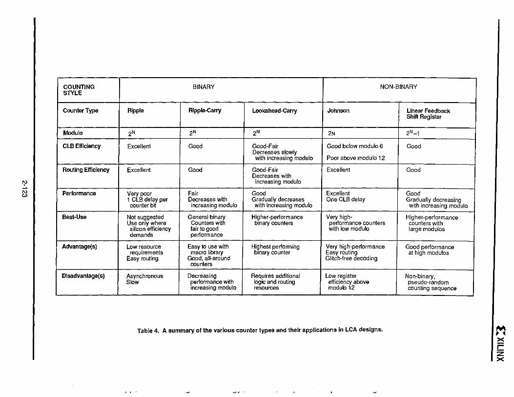
Table 5 lists the various counter types and associated comments. It should prove helpful when determining which counter to use for an application. In some applications, overall performance may be the critical need. With others, absolute resource efficiency may by required. With more than one possible implementation available, the designer can tailor the logic to custom-fit his application instead of wasting resources on Circuitry that is not used for his application.

TECHNICAL SOURCES:

1. Messina, A. Considerations for Non-Binary Counter Applications. Computer Design, November 1972. pp. 99-101.

2-120

RESET

CLOCK

0010023 17a

l:XILlNX

~ __________________________________________________ ~ TERMINAL COUNT INPUTS

I I FROM MODULO-3

MODULO-3JOH.~S?.~.~O.U~.TE~ ............................... :... .. : ............... 1 ................ ~O~.NSONCOUNTER ,,: : . I" .. ... .. .. ::~

r--'U. :.: ;:': 1 ! I:! ,:: : : 1"1 - ::: MODULO-15

'-- D a 1 i 0 Q r"-;'=\L:~~,_J b~~~~AL

b=:::,,",JJ l1::",J r - ---------------------------------------------, I . ,,:: I

I f~ i I r~"~~Jt.gCl} 1-----1~H~·;;;..::: -!:~::::D=::Q:;';:: ~,~;.. D a I-}J "'-TERMINAL COUNT INPUTS

:,:' .::::: FROM MODULO-5 \i: iii. LFSR COUNTER

.--1> rt ~RD r-:::~ I> •.. : .•... : . I.:: ~r- :i: .--LLe=::jt::::::=:::::::=~=::::t~=:::J:=:t:=::J 1,,-p

MODULO-5 LFSR COUNTER --------------------------------------------------~

Figure 17a. A modulo-15 heterodyne counter built from a modulo-5 LFSR Counter and a modulo-3 Johnson counter

2-121

I\) I ~

I\) I\)

0010023178

RESET

MODULO-3 TERMINAL COUNT

MODULO-5 TERMINAL COUNT

HETERODYNE TERMINAL COUNT

MODULO-15

CLOCK

I 0 ! 1 2131-4- fs-T-s- 1 -7- r 8 -,-9- T 1o-Tfi 1-12- 1 13- , 14 15! 1 I 2

~~--------------------~--__ ~~n n n n n~: __ ________ ~n n [l~: __

_ ------ _n _ _ n_: _

Figure 17b. Timing diagram for the modulo-1S heterodyne counter. Notice that the terminal counts from the first two counters combine to produce a third terminal count every fifteen clock cycles.

(") o C :l -CD ... ~ III 3

"C CD UI

F\) I .......

F\) c.:l

COUNTING STYLE

Counter Type

Modulo

CLB Efficiency

Routing Efficiency

Performance

Best-Use

Advantage(s)

Disadvantage(s)

BINARY NON-BINARY

Ripple Ripple-Carry Lookahead-Carry Johnson Linear Feedback Sh itt Reg ister

2N 2N 2N 2N 2N_1

Excellent Good Good-Fair Good below modulo 6 Good Decreases slowly with increasing modulo Poor above modulo 12

Excellent Good Good-Fair Excellent Good Decreases with increasing modulo

Very poor Fair Good Excellent Good 1 CLB delay per Decreases with Gradually decreases One CLB delay Gradually decreasing counter bit increasing modulo with increasing modulo with increasing modulo

Not suggested General binary Higher-performance Very high- Higher-performance Use only where Counters with binary counters performance counters counters with silicon efficiency fair to good with low modulo large modulos demands performance

Low resource Easy to use with Hi!iJhest performing Very high-performance Good performance requirements macro library binary counter Easy routing at high modulos

Easy routing Good, all-around Glitch-free decoding counters

Asynchronous Decreasing Requires additional Low register Non-binary, Slow performance with logic and routing efficiency above pseudo-random

increasing modulo resources modulo 12 counting sequence

Table 4. A summary of the various counter types and their applications in LCA designs. M >< C z ><