Counterparty Credit Risk & Central Clearing

Credit Risk SummitLondon

18 September2009

Josh Danziger Ed Parcell

Counterparty credit risk management

Credit Rates etcCredit Rates etc

No CSA Eg, monolines ―o CS g,

CSA on downgrade

Eg, AIGHighly‐rated counterpartiesdowngrade counterparties

CSA Interbank business Interbank business

100% collateral

Credit‐linked notes Structured notes

Central clearing

ICE, Eurex, Clearnet Swapclear

2

Counterparty credit risk 

90

1002500

70

80

90

2000

50

601500

MBIA (LH axis)

30

401000ABX06‐2 (RH axis)

10

20500

A hi hl l t d t t ith CSA th dit iti ti

00

Sep 05 Mar 06 Sep 06 Mar 07 Sep 07 Mar 08 Aug 08 Mar 09 Aug 09 Mar 10

3

• A highly correlated counterparty with no CSA or other credit mitigation.

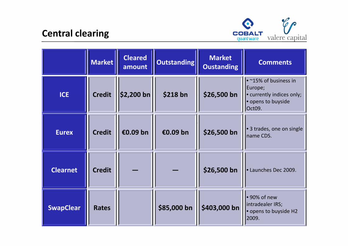
Central clearing

MarketClearedamount

OutstandingMarket 

OustandingComments

amount Oustanding

ICE Credit $2 200 bn $218 bn $26 500 bn

• ~15% of business in  Europe; • currently indices only;ICE Credit $2,200 bn $218 bn $26,500 bn currently indices only;• opens to buysideOct09.

Eurex Credit €0.09 bn €0.09 bn $26,500 bn • 3 trades, one on single name CDS.

Clearnet Credit ― ― $26,500 bn • Launches Dec 2009.

SwapClear Rates $85 000 bn $403 000 bn

• 90% of new intradealer IRS; 

4

SwapClear Rates $85,000 bn $403,000 bn ;• opens to buyside H2 2009.

The push for central clearing

• Correlated counterparties.  Banks have concentrated on allocating derivatives line according to creditworthiness, but we know from history of monolines that creditworthiness conditioned on situations where derivatives are in the money is more relevantconditioned on situations where derivatives are in the money is more relevant. 

... although buyside entities may not all move to central clearing.

• Close‐out on bankruptcy.  Lehman bankruptcy highlighted complexity of managing derivatives close outs on default of highly connected counterpartyclose‐outs on default of highly connected counterparty ...

... although as it happens Lehman close-outs ran smoothly.

• Market transparency.  Weak transaction reporting left authorities unaware of huge positions amassed by AIG FPamassed by AIG FP ...

... although as it happens CDS on subprime executed by AIG FP would not be suitable for central clearing.

• Aid to settlement efficiency Settlement backlogs in CDS market have in the past reachedAid to settlement efficiency.  Settlement backlogs in CDS market have in the past reached unacceptable levels, and dealers have at times done a poor job of properly unwinding trades after closing out ...

... although as it happens reduction of outstanding CDS from >$60tn to <$30tn has been li h d tl th h t d i i th th th h CCPaccomplished mostly through trade compression services rather than through CCPs.

• Retention of trading liquidity in a crisis.  Cutting derivatives lines because of increased credit risk in the crisis lead to market illiquidity ...

lth h if CCP dit lit t b i l ll d i t ti th th

5

... although if CCP credit quality were ever to be seriously called into question then there would be severe implications for market liquidity.

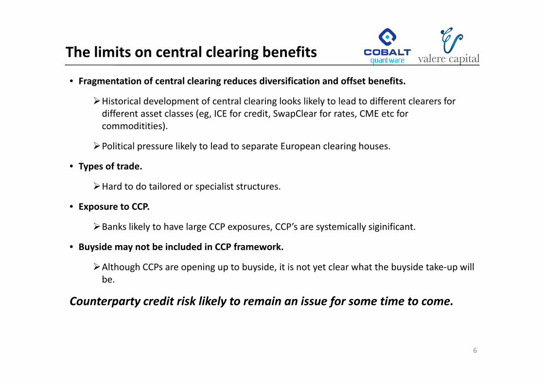
The limits on central clearing benefits

• Fragmentation of central clearing reduces diversification and offset benefits. 

Historical development of central clearing looks likely to lead to different clearers for p g ydifferent asset classes (eg, ICE for credit, SwapClear for rates, CME etc for commoditities).

Political pressure likely to lead to separate European clearing houses.Political pressure likely to lead to separate European clearing houses.

• Types of trade. 

Hard to do tailored or specialist structures.

• Exposure to CCP.  

Banks likely to have large CCP exposures, CCP’s are systemically siginificant.

• Buyside may not be included in CCP framework.

Although CCPs are opening up to buyside, it is not yet clear what the buyside take‐up will bebe.

Counterparty credit risk likely to remain an issue for some time to come.

6

Pricing and hedging counterparty risk

• Complexity of counterparty risk:

• Netting;

• No CSA/ CSA on downgrade/ “regular” CSA;

• CSA threshold issues.

• Modelling techniques.

• Focus on CDS to illustrate issues.

• Does counterparty‐ or self‐hedging change things?

7

Counterparty‐ and self‐hedging

Counterparty hedging Self hedging

• We wish to buy protection on RefCo • We wish to sell protection on RefCo (trading (trading at 700) from CPCo (trading at 500).   at 700); we ourselves are trading at 500. 

• Our model determines that correlation between RefCo and CPCo means we agree to

• Our model determines that correlation between RefCo and ourselves means webetween RefCo and CPCo means we agree to 

pay only 400 for protection rather than 700.between RefCo and ourselves means we agree to accept only 400 for protection rather than 700.

• To hedge our counterparty risk we will have • To hedge our self risk we will sell protectionTo hedge our counterparty risk we will have to incur the expense of buying protection on a delta amount of CPCo.

To hedge our self risk we will sell protection on a delta amount of our own name (perhaps through buying a CLN, or  buying our own bonds).

• We should also be aware that we have less than 100% delta on RefCo. 

• We should also be aware that we have less than 100% delta on RefCo. 

• Failure to buy protection on CPCo may make our protection look cheap (400 rather than 700), but we are running the risk of CPCowidening out and perhaps failing

• Failure to sell protection on ourselves leaves us exposed to our own name: if it tightened in to double digits we might find ourselves 300 basis points under water without any

8

widening out, and perhaps failing. 300 basis points under water, without any change in RefCo.

Impact of counterparty‐ or self‐hedging

• Hedging counterparty risk enhances correlation• Hedging counterparty risk enhances correlation between protection seller and reference entity (eg, monolines). 

• Hedging self risk may involve overcoming funding and regulatory hurdles:

Buying own bonds (requires funding); or

Selling own protection‐‐‐eg, through creating CLN (requires funding)(requires funding).

Either way will tend to diminish correlation between self and reference entity on which yprotection sold ...

.... But makes poor trades much more painful!

9

Credit Value Adjustment (CVA)

• Adjusts valuation of a trade or portfolio for the possibility of self or counterparty default.

• Prior to credit crunch CVA was typically unilateral, incorporating only the possibility of yp y , p g y p ycounterparty default, with institutions assuming themselves to be default‐free.

• If the counterparty has low credit quality then the CVA is larger, and the NPV of the trade is less positive, or more negative. Other institutions would require a lower spread to buyless positive, or more negative. Other institutions would require a lower spread to buy protection from that counterparty, and would sell protection at a higher spread.

• During 2008 as credit quality of financial institutions fell,  all buyers offered lower spreads, and all sellers demanded higher spreads leading to a loss of liquidityall sellers demanded higher spreads, leading to a loss of liquidity.

• CVAs that incorporate the possibility of either counterparty defaulting avoid this. “Bilateral” CVAs are symmetric, so if two counterparties have the same view of the reference entity’s, their own and each others’ credit quality they will agree on the CVAtheir own and each others  credit quality, they will agree on the CVA.

• CVA can be decomposed into two parts:

• Asset Charge: NPV of counterparty defaulting when trade is in the moneyAsset Charge: NPV of counterparty defaulting when trade is in the money

• Liability Benefit: NPV of us defaulting when the trade is out of the money

10

Calculating CVA

• For a general trade or portfolio

[ ] dtttPtttVtBERRT

)(|)()0()1(ChargeAsset >>∫ + ττττ[ ][ ] dtttPtttVtBERR

dtttPtttVtBERR

CS

T

CSS

SCSCC

),(,|)(),0()1(BenefitLiability

),(,|)(),0()1(ChargeAsset

0

0

>=>=−=

>=>=−=

∫∫

− ττττ

ττττ

• Where

RRC= Recovery rate of counterpartyRRS = Recovery rate of selfSB(0,t) = Discount factor from 0 to tV(t) = Valuation of trade/portfolio at time t (excluding counterparty risk)V+(t) = max[0,V(t)], V‐(t) = min[0,V(t)]τ = Default time of counterpartyτC = Default time of counterpartyτs = Default time of self

Counterparty Valuation Adjustment (CVA). 2009. Shahram Alavian, Jie Ding, Peter Whitehead & Leonardo d

11

Laudicina.

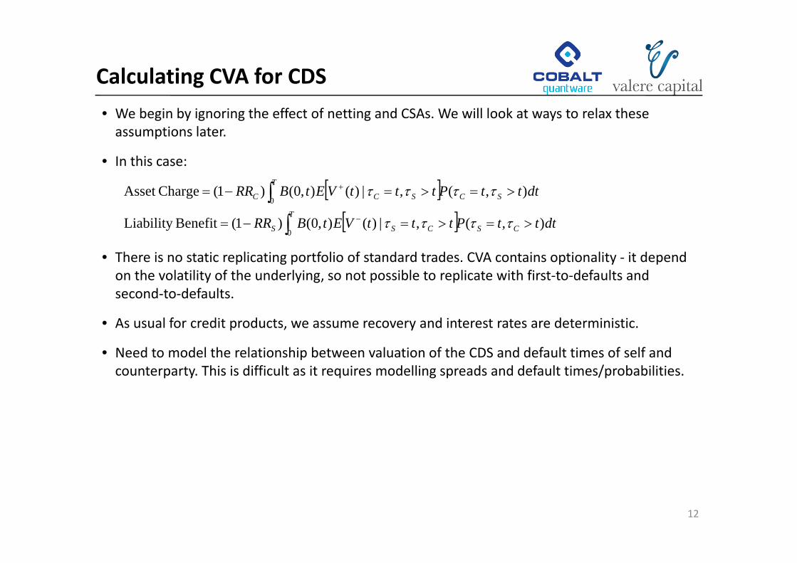
Calculating CVA for CDS

• We begin by ignoring the effect of netting and CSAs. We will look at ways to relax these assumptions later.

[ ][ ]

dtttPtttVEtBRRT

SC

T

SCC ),(,|)(),0()1(ChargeAsset 0

>=>=−=

∫∫ + ττττ

• In this case:

• There is no static replicating portfolio of standard trades. CVA contains optionality ‐ it depend on the volatility of the underlying, so not possible to replicate with first‐to‐defaults and 

[ ] dtttPtttVEtBRR CSCSS ),(,|)(),0()1(BenefitLiability 0

>=>=−= ∫ − ττττ

y y g, p psecond‐to‐defaults.

• As usual for credit products, we assume recovery and interest rates are deterministic.

• Need to model the relationship between valuation of the CDS and default times of self and counterparty. This is difficult as it requires modelling spreads and default times/probabilities.

12

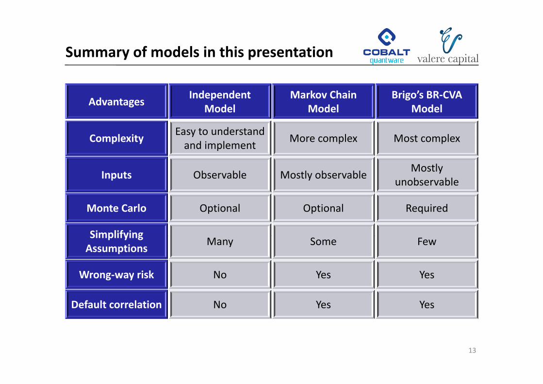
Summary of models in this presentation

AdvantagesIndependent 

d lMarkov Chain 

d lBrigo’s BR‐CVA 

d lAdvantages

Model Model Model

ComplexityEasy to understand and implement

More complex Most complexand implement

Inputs Observable Mostly observableMostly 

unobservable

Monte Carlo Optional Optional Required

SimplifyingSimplifying Assumptions

Many Some Few

Wrong‐way risk No Yes Yesg y

Default correlation  No Yes Yes

13

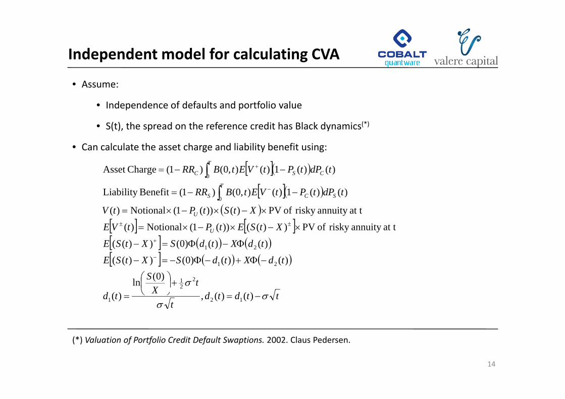
Independent model for calculating CVA

• Assume:

• Independence of defaults and portfolio valuep p

• S(t), the spread on the reference credit has Black dynamics(*)

• Can calculate the asset charge and liability benefit using:

[ ]( )

[ ]( ) tdPtPtVEtBRR

tdPtPtVEtBRR

SC

T

S

CS

T

C

−−=

−−=

−

+

∫∫

)()(1)(),0()1(BenefitLiability

)()(1)(),0()1(ChargeAsset

0

0

( )[ ] [ ][ ] ( ) ( )tdXtdSXtSE

XtSEtPtVE

XtStPtV

U

U

Φ−Φ=−

×−×−×=

×−×−×=

+

±±

∫

)()()0())((

at tannuity risky of PV))(())(1(Notional)(

at tannuity risky of PV)())(1(Notional)(0

[ ] ( ) ( )[ ] ( ) ( )

tX

StdXtdSXtSE

tdXtdSXtSE

σ+⎟⎠⎞

⎜⎝⎛

−Φ+−Φ−=−

ΦΦ=−

)0(ln

)()()0())(()()()0())((

221

21

21

ttdtdt

Xtd σσ

−=⎠⎝= )()(,)( 121

14

(*) Valuation of Portfolio Credit Default Swaptions. 2002. Claus Pedersen.

Example CVA (Independent model)

• Model Inputs

• Bought protection

• Model Outputs:

• PV (excluding CVA) = $1,176kg p

• Notional = $10MM

• Maturity = 5 years

• CDS spread 500bps

( g ) $ ,

• Liability benefit = ‐$8k

• Asset Charge = $58k• CDS spread = 500bps

• Interest rate = 2%

• Volatility = 80%

• PV (including CVA) = $1,126k

Recovery5y Market Spread

Self 10% 120bpsSelf 10% 120bpsUnderlying 40% 850bpsCounterparty 10% 180bps

15

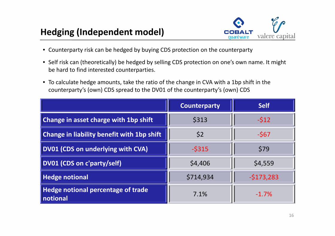
Hedging (Independent model)

• Counterparty risk can be hedged by buying CDS protection on the counterparty

• Self risk can (theoretically) be hedged by selling CDS protection on one’s own name. It might ( y) g y g p gbe hard to find interested counterparties.

• To calculate hedge amounts, take the ratio of the change in CVA with a 1bp shift in the counterparty’s (own) CDS spread to the DV01 of the counterparty’s (own) CDScounterparty s (own) CDS spread to the DV01 of the counterparty s (own) CDS

Counterparty Self

Ch i t h ith 1b hift $313 $12Change in asset charge with 1bp shift $313 ‐$12

Change in liability benefit with 1bp shift $2 ‐$67

DV01 (CDS on underlying with CVA) ‐$315 $79

DV01 (CDS on c'party/self) $4,406 $4,559

Hedge notional $714,934 ‐$173,283

Hedge notional percentage of trade notional

7.1% ‐1.7%

16

notional

CVA sensitivities (Independent model)

80,000 

vs self spread80,000 

vs counterparty spread

20 000

0 

20,000 

40,000 

60,000 

0 00% 0 50% 1 00% 1 50% 2 00% 2 50% 3 00% 20 000

0 

20,000 

40,000 

60,000 

0 00% 1 00% 2 00% 3 00% 4 00% 5 00%

‐80,000 

‐60,000 

‐40,000 

‐20,000 0.00% 0.50% 1.00% 1.50% 2.00% 2.50% 3.00%

‐80,000 

‐60,000 

‐40,000 

‐20,000 0.00% 1.00% 2.00% 3.00% 4.00% 5.00%

60,000 

80,000 

vs reference entity spread

60,000 

80,000 

vs volatility

‐20,000 

0 

20,000 

40,000 

,

0% 2% 4% 6% 8% 10% 12% ‐20,000 

0 

20,000 

40,000 

,

0% 25% 50% 75% 100% 125% 150%

‐80,000 

‐60,000 

‐40,000 

‐80,000 

‐60,000 

‐40,000 

17

Comments on CVA sensitivities

• The CVA is sensitive to the spread of the  reference entity. As a result our delta is less than 1 (vs the CDS excluding counterparty risk effects).

• Increases in the counterparty spread increase the asset charge, reducing trade valuation.

• Increases in self spread increase the size of the liability benefit, increasing the trade valuation.  In general we expect increases in self spread have the opposite effect on trade valuation ofIn general we expect increases in self spread have the opposite effect on trade valuation of increases in counterparty spread.

• Here the trade pays 500bps vs the market spread of 850bps. The liability option is very out of the money so the liability benefit is small vs the asset charge and the effect of counterpartythe money, so the liability benefit is small vs the asset charge and the effect of counterparty spread is more important than self spread.

18

Incorporating correlation

• Example of the effect of correlation:

• Suppose we have bought protection on a reference entity and there is positive pp g p y pcorrelation between the credit quality of the reference entity and the counterparty.

• The counterparty is most likely to default when bought protection is most valuable.[ E(V+|τc=t,τs>t) will be higher than in the independent case. ]

• We would expect the asset charge will be higher.

19

Markov Chain Model

Self , then underlyingλ'U

Self defaulted (S) underlying 

defaulted (SU)U

Underlying d f lt d (U)

(S)

λUNo defaults 

(0)

Counterparty, then λ'U

Counterparty d f l d (C)

defaulted (U)U(0)

• Correlation from increased default intensity for underlying if counterparty or self default.

underlying defaulted (CU)

Udefaulted (C)

Correlation from increased default intensity for underlying if counterparty or self default.

• Calibrate by setting λ'U = αλU (choose α based on historical data), and solving for λU so that the default‐free CDS on the underlying reprices the market.

• Possible extensions:• Possible extensions:

• Underlying default intensity different in S or C (e.g. if counterparty less systemically important).

• More than one underlying (e g for portfolio of CDS)

20

• More than one underlying (e.g. for portfolio of CDS).

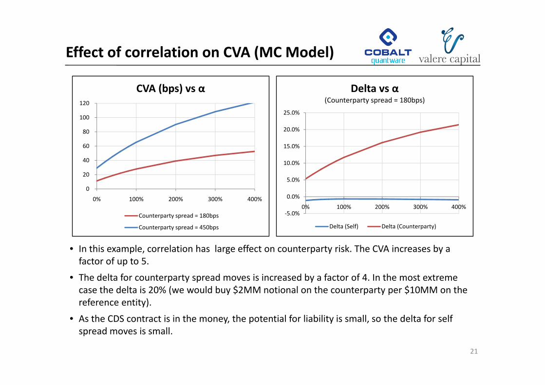
Effect of correlation on CVA (MC Model)

120 

CVA (bps) vs α Delta vs α(Counterparty spread = 180bps)

60 

80 

100 

0

15.0%

20.0%

25.0%

0 

20 

40 

5.0%

10.0%

0% 100% 200% 300% 400%

Counterparty spread = 180bps

Counterparty spread = 450bps

‐5.0%

0.0%

0% 100% 200% 300% 400%

Delta (Self) Delta (Counterparty)

• In this example, correlation has  large effect on counterparty risk. The CVA increases by a factor of up to 5.

• The delta for counterparty spread moves is increased by a factor of 4. In the most extremeThe delta for counterparty spread moves is increased by a factor of 4. In the most extreme case the delta is 20% (we would buy $2MM notional on the counterparty per $10MM on the reference entity). 

• As the CDS contract is in the money, the potential for liability is small, so the delta for self 

21

y p yspread moves is small.

Brigo’s BR‐CVA Model (Part 1)

• For each obligor, unconditional default intensities are simulated using an independent CIR process plus a deterministic function of time, used to fit to market spreads. These intensities are integrated to calculate unconditional default probabilities for each name over timeare integrated to calculate unconditional default probabilities for each name over time.

0 2000

0.3000

Default Intensities

Y00.1500

0.2000

Cumulative default probabilities

C0

0.0000

0.1000

0.2000

0.00 1.00 2.00 3.00 4.00 5.00

Y0

Y1

Y2 0.0000

0.0500

0.1000

0.00 1.00 2.00 3.00 4.00 5.00

C0

C1

C2

• A uniform variate for each name determines default time(eg the red dot has U0 = 0.097, U1 = 0.174, U2 = 0.046)

0 8

1.0

0 8

1.0

0.0

0.2

0.4

0.6

0.8

U1

0.0

0.2

0.4

0.6

0.8

U2

• Default of obligor i occurs when Ui > Ci. (eg the red dot indicates obligor 2 defaults at time 3.13 and obligor 1 would default shortly after time 5).

0.0 0.2 0.4 0.6 0.8 1.0U0

0.0 0.2 0.4 0.6 0.8 1.0U0

22

Bilateral counterparty risk valuation with stochastic dynamical models and application to CDS.2009. Damiano Brigo & Agostino Capponi.

Brigo’s BR‐CVA Model (Part 2)

• If the counterparty (2) defaults before either us or the underlying and prior to the maturity of the CDS, and the value of the CDS is positive at the default time, the CDS value contributes to the asset charge for that simulationthe asset charge for that simulation.

• If we (0) default before either the counterparty or the underlying and prior to the maturity of the CDS, and the value of the CDS is negative at the default time, the CDS value contributes to th li bilit b fit f th t i l tithe liability benefit for that simulation.

• The CDS must be valued conditional on the value of the uniform variate representing the defaulting obligor. The conditional probabilities of default can be calculated by

• The easiest way to approximate the cumulative density function of the the integrated CIR

( ) 101|

1

0 10 1 ;|)()(exp01

duuufFutdttYP UUt

T

∫ ∫ ⎟⎠⎞⎜

⎝⎛ >⎟

⎠⎞⎜

⎝⎛ −− ψ

• The easiest way to approximate the cumulative density function of the the integrated CIR intensity process is using:

YjYYdtkdttYPkjiIti

δδδ

⎟⎠⎞⎜

⎝⎛ =≤= ∫ )0(|)(),,(

0

( )( )YjYYjYjtYPjjM

jjMjkjIkjiIj

δδδδ =+′−′∈=′

′−′−=∑′

)0(|)(,)()(),(

),(),,1(),,(

21

21

23

Incorporating CSAs

• CSAs with no threshold

• Remaining risk is jump risk – hard to model, little available data.g j p ,

• CSAs with a threshold

• Independent and Markov Chain models: For liability benefit, model V‐(t) as a put on V(t) at 0bps and a call at ‐Threshold / [Notional × (1‐PU (t) × PV of risky annuity].

• BR‐CVA and Monte Carlo model: Restrict V(t) to below the threshold in each simulation.

CSA ith ti t i d t d l ti• CSAs with rating triggers – need to model a rating process.

• Markov Chain model: Incorporate extra states for downgrade . Self can default directly, or default from downgraded state with different intensities.

• BR‐CVA model: Imply spreads from current values of CIR processes, and from these a rating process based on implied spread. Restrict V(t) within a simulation if rating trigger is breached.

24

Incorporating netting

• Difficult because need to model spread evolution and default states for a portfolio of obligors.

• Markov Chain model

• Can extend number of states to incorporate each possible set of defaults.

• Can simply transition matrix by assuming intensity on each obligor is a function of original intensity and number of defaults.

• Quickly becomes unwieldy to do analytically. Monte Carlo is feasible.

BR CVA d l• BR‐CVA model

• Simulate a CIR process correlated uniform for each underlying.

• If counterparty or self default before maturity of portfolio value entireIf counterparty or self default before maturity of portfolio, value entire portfolio, conditional on values of uniform variates of all defaulted obligors, including counterparty/self.

25

Conclusion

• With the rise in credit spreads since 2007, and several high‐profile defaults, credit risk has been an increasingly important issue.

• Central clearing alleviates some of the systemic impact of credit risk, but it remains an issue for exotic trades, and particularly for the buy‐side.

• Credit risk is incorporated by including a credit value adjustment when pricing a deal. In theCredit risk is incorporated by including a credit value adjustment when pricing a deal. In the past this has focussed mostly on the risk of the counterparty defaulting. More recently it has been necessary to factor in one's own risk

• Calculating credit value adjustment for CDS trades requires modelling the default and spreadCalculating credit value adjustment for CDS trades requires modelling the default and spread volatility of the reference entity, the defaults of the counterparty and ourself, and the relation between these.

• The main factor driving the credit value adjustment is the correlation between the spread of• The main factor driving the credit value adjustment is the correlation between the spread of the reference entity and counterparty or self defaulting ‐ high positive correlation would tend to cause bought protection to be worth less.

• Finall e looked at f t re e tensions to e isting models to deal ith more intricate feat res• Finally, we looked at future extensions to existing models to deal with more intricate features of CSAs.

26

Contacts

Josh Danziger josh.danziger@valere‐capital.com

Josh Danziger is a Principal of Valere Capital Partners LLP, a specialist fixed‐income consultancy based in London.  Prior to this he was Head of Structured Products at Royal Bank of Canada, responsible for structured rates, inflation, credit derivatives and principal finance.  His PhD at Cambridge University concerned the computer modeling of the chemical interactions between proteins and drugs at a molecular level.

Ed Parcell ed.parcell@cobaltquantware.com

Ed Parcell is Managing Director of Cobalt Quantware, a consultancy providing quantitative modelling andEd Parcell is Managing Director of Cobalt Quantware, a consultancy providing quantitative modelling and software development expertise. Previously he has worked at Brevan Howard Asset Management, ReochCredit Partners and Fitch Ratings on market valuation analytics for credit derivatives.

27