coupled-oscillator based active-array antennas...2011/08/04 · coupled-oscillator based...
TRANSCRIPT
Coupled-Oscillator Based Active-Array Antennas
Ronald J. Pogorzelski and Apostolos Georgiadis
Jet Propulsion Laboratory
California Institute of Technology
DEEP SPACE COMMUNICATIONS AND NAVIGATION SERIES
DEEP SPACE COMMUNICATIONS AND NAVIGATION SERIES
Issued by the Deep Space Communications and Navigation Systems Center of Excellence
Jet Propulsion Laboratory California Institute of Technology
Joseph H. Yuen, Editor-in-Chief
Published Titles in this Series
Radiometric Tracking Techniques for Deep-Space Navigation Catherine L. Thornton and James S. Border
Formulation for Observed and Computed Values of Deep Space Network Data Types for Navigation Theodore D. Moyer
Bandwidth-Efficient Digital Modulation with Application to Deep-Space Communications Marvin K. Simon
Large Antennas of the Deep Space Network William A. Imbriale
Antenna Arraying Techniques in the Deep Space Network David H. Rogstad, Alexander Mileant, and Timothy T. Pham
Radio Occultations Using Earth Satellites: A Wave Theory Treatment
William G. Melbourne
Deep Space Optical Communications Hamid Hemmati, Editor
Spaceborne Antennas for Planetary Exploration William A. Imbriale, Editor
Autonomous Software-Defined Radio Receivers for Deep Space Applications Jon Hamkins and Marvin K. Simon, Editors
Low-Noise Systems in the Deep Space Network Macgregor S. Reid, Editor
Coupled-Oscillator Based Active-Array Antennas Ronald J. Pogorzelski and Apostolos Georgiadis
Coupled-Oscillator Based Active-Array Antennas
Ronald J. Pogorzelski and Apostolos Georgiadis
Jet Propulsion Laboratory
California Institute of Technology
DEEP SPACE COMMUNICATIONS AND NAVIGATION SERIES

Coupled-Oscillator Based Active-Array Antennas
June 2011
A portion of this publication was prepared at the Jet Propulsion Laboratory, California Institute of Technology, under a contract with the National Aeronautics and Space Administration. The balance of this publication was prepared under contract with the Ministry of Science and Innovation Spain and the European COST Action IC0803 RF/Microwave Communication Subsystems for Emerging Wireless Technologies.
Reference herein to any specific commercial product, process, or service by trade name, trademark, manufacturer, or otherwise, does not constitute or imply its endorsement by the United States Government or the Jet Propulsion Laboratory, California Institute of Technology.
v
Table of Contents Dedication ................................................................................................ ix Foreword ................................................................................................. xi Preface ................................................................................................... xiii Acknowledgements ................................................................................ xvii Authors ................................................................................................... xix
Part I: Theory and Analysis ........................................... 1
Chapter 1 Introduction – Oscillators and Synchronization ...... 1
1.1 Early Work in Mathematical Biology and Electronic Circuits ................................................................................ 1
1.2 van der Pol’s Model ............................................................ 3
1.3 Injection Locking (Adler’s Formalism) and Its Spectra (Locked and Unlocked) ...................................................... 5
1.4 Mutual Injection Locking of Two Oscillators ................. 19
1.5 Conclusion ........................................................................ 24
Chapter 2 Coupled Oscillator Arrays – Basic Analytical Description and Operating Principles .................. 25
2.1 Fundamental Equations ................................................... 26
2.2 Discrete Model Solution (Linearization and Laplace Transformation) ................................................................ 29
2.3 Steady-State Solution ...................................................... 35
2.4 Stability of the Phase Solution in the Full Nonlinear Formulation ....................................................................... 39
2.5 External Injection Locking ............................................... 44
2.6 Generalization to Planar Arrays ...................................... 48
2.7 Coupling Networks ........................................................... 52
2.8 Conclusion ........................................................................ 64
Chapter 3 The Continuum Model for Linear Arrays ................ 65
vi Table of Contents
3.1 The Linear Array without External Injection .................. 66
3.2 The Linear Array with External Injection ........................ 79
3.3 Beam-steering via End Detuning .................................... 91
3.4 Beam-steering via End Injection ..................................... 93
3.5 Conclusion ...................................................................... 100
Chapter 4 The Continuum Model for Planar Arrays ............. 101
4.1 Cartesian Coupling in the Continuum Model without External Injection .............................................. 101
4.2 Cartesian Coupling in the Continuum Model with External Injection ........................................................... 109
4.3 Non-Cartesian Coupling Topologies ............................ 116
4.4 Conclusion ...................................................................... 135
Chapter 5 Causality and Coupling Delay ............................... 137
5.1 Coupling Delay ............................................................... 137
5.2 The Discrete Model with Coupling Delay ..................... 139
5.3 The Continuum Model with Coupling Delay ................ 144
5.4 Beam Steering in the Continuum Model with Coupling Delay ............................................................... 157
5.5 Conclusion ...................................................................... 171
Part II: Experimental Work and Applications ........... 173
Chapter 6 Experimental Validation of the Theory ................. 173
6.1 Linear-Array Experiments ............................................. 173
6.2 Planar Array Experiments ............................................. 184
6.3 Receive Array Experiments ........................................... 197
6.4 Phase Noise .................................................................... 206
6.5 The Unlocked State ........................................................ 209
6.6 Conclusion ...................................................................... 211
vii Table of Contents
Part III: Nonlinear Behavior ....................................... 213
Chapter 7 Perturbation Models for Stability, Phase Noise, and Modulation .................................................... 213
7.1 Preliminaries of Dynamical Systems ............................ 214 7.1.1 Introduction to Stability Analysis of Nonlinear
Dynamical Systems ..................................................... 217 7.1.2 Equilibrium Point ........................................................ 217 7.1.3 Periodic Steady State ................................................... 218 7.1.4 Lyapunov Exponents ................................................... 219
7.2 Bifurcations of Nonlinear Dynamical Systems ............ 220 7.2.1 Bifurcations of Equilibrium Points .............................. 220 7.2.2 Bifurcations of Periodic Orbits.................................... 222
7.3 The Averaging Method and Multiple Time Scales ....... 224
7.4 Averaging Theory in Coupled Oscillator Systems ...... 225
7.5 Obtaining the Parameters of the van der Pol Oscillator Model ............................................................. 229
7.6 An Alternative Perturbation Model for Coupled-Oscillator Systems ......................................................... 232
7.7 Matrix Equations for the Steady State and Stability Analysis ........................................................................... 236
7.8 A Comparison between the Two Perturbation Models for Coupled Oscillator Systems ...................... 240
7.9 Externally Injection-Locked COAs ................................ 241
7.10 Phase Noise .................................................................... 244
7.11 Modulation ...................................................................... 250
7.12 Coupled Phase-Locked Loops ...................................... 252
7.13 Conclusion ...................................................................... 255
Chapter 8 Numerical Methods for Simulating Coupled Oscillator Arrays .................................................. 257
8.1 Introduction to Numerical Methods .............................. 258 8.1.1 Transient Simulation ................................................... 258 8.1.2 Harmonic Balance Simulation..................................... 260 8.1.3 Conversion Matrix ....................................................... 261 8.1.4 Envelope Transient Simulation ................................... 262
viii Table of Contents
8.1.5 Continuation Methods ................................................. 263
8.2 Obtaining Periodic Steady-State Solutions of Autonomous Circuits in Harmonic-Balance Simulators ....................................................................... 264
8.3 Numerical Analysis of a Voltage-Controlled Oscillator ......................................................................... 266
8.4 Numerical Analysis of a Five-Element Linear Coupled-Oscillator Array ............................................... 272
8.5 Numerical Analysis of an Externally Injection- locked Five-Element Linear Coupled-Oscillator Array ................................................................................ 280
8.6 Harmonic Radiation for Extended Scanning Range ... 282
8.7 Numerical Analysis of a Self-Oscillating Mixer ........... 285
8.8 Conclusion ...................................................................... 290
Chapter 9 Beamforming in Coupled-Oscillator Arrays ........ 291
9.1 Preliminary Concepts of Convex Optimization ........... 291
9.2 Beamfoming in COAs .................................................... 295
9.3 Stability Optimization of the Coupled-Oscillator Steady-State Solution .................................................... 302
9.4 Multi-Beam Pattern Generation Using Coupled-Oscillator Arrays ............................................. 305
9.5 Control of the Amplitude Dynamics ............................. 309
9.6 Adaptive Coupled-Oscillator Array Beamformer ........ 311
9.7 Conclusion ...................................................................... 314
Chapter 10 Overall Conclusions and Possible Future Directions ............................................................. 315
References ............................................................................... 319
Acronyms and Abbreviations ................................................. 335

ix
We dedicate this book to our wives,
Barbara and Ana,
who sustained us in this endeavor.

x
xi
Foreword
The Deep Space Communications and Navigation Systems Center of Excellence (DESCANSO) was established in 1998 by the National Aeronautics and Space Administration (NASA) at the California Institute of Technology’s Jet Propulsion Laboratory (JPL). DESCANSO is chartered to harness and promote excellence and innovation to meet the communications and navigation needs of future deep-space exploration.
DESCANSO’s vision is to achieve continuous communications and precise
navigation—anytime, anywhere. In support of that vision, DESCANSO aims to seek out and advocate new concepts, systems, and technologies; foster key technical talents; and sponsor seminars, workshops, and symposia to facilitate interaction and idea exchange.
The Deep Space Communications and Navigation Series, authored by
scientists and engineers with many years of experience in their respective fields, lays a foundation for innovation by communicating state-of-the-art knowledge in key technologies. The series also captures fundamental principles and practices developed during decades of deep-space exploration at JPL. In addition, it celebrates successes and imparts lessons learned. Finally, the series will serve to guide a new generation of scientists and engineers. Joseph H. Yuen DESCANSO Leader

xii

xiii
Preface
This book is a compilation of research results obtained primarily over the past two decades in the application of groups of oscillators coupled in various configurations to the excitation of phased-array antennas. Much of the work was carried out at the Jet Propulsion Laboratory of the California Institute of Technology under contract with the National Aeronautics and Space Administration (NASA) building on the early work at the University of Massachusetts, Cornell University, and the University of California, Santa Barbara. More recent work at several institutions in Spain and especially at the Centre Tecnologic de Telecomunicacions de Catalunya (CTTC), as well as a variety of institutions across Europe and Asia is also described. A motivation for much of this work was the promise of a method of providing beam agility at electronic speed that is simpler than the conventional method of using a phase shifter at each element or module and controlling these phase shifters in a coordinated manner. More generally, however, the effort has focused on the integration of transmitter, receiver, and antenna including the beam-steering function in a single planar package.
The intended audience for the book comprises primarily designers of
phased-array antennas and the associated electronics, but the book may also be of interest to those who may, through understanding the principles presented, envision other innovative applications of oscillator arrays such as distribution of timing signals and phase locking in general. In the same way, graduate students may find inspiration for research work leading to theses or dissertations based on extending the work described here.
With regard to the references, as a general rule we have used peer reviewed
archival journal articles and not conference presentations in the interest of ease
xiv Preface
of access. We have, however, made a few exceptions in this regard in cases of very recent work that, as far as we know, has not yet appeared in the peer-reviewed literature and in one case for the use of figures with proper attribution. We have endeavored to present a comprehensive treatment of the work in this field to date but recognize that we cannot be sure that we are aware of everyone in the world with interest in and contributions to this fascinating area of research. We, therefore, extend apologies to any who feel their work has been slighted in any way. Be assured it was unintentional.
The book begins with a note concerning the early use of coupled oscillators
in the field of mathematical biology wherein researchers used them as an artifice in representing the behavior of neurons in what is known as a central pattern generator in a manner amenable to mathematical analysis. The application to phased array antennas owes its origin primarily to Karl Stephan at the University of Massachusetts [1] [2] [3] and to Richard C. Compton at Cornell and his student, Robert A. York. [4] [5] [6] [7] However, the modern emphasis on the study of the dynamics of such arrays was inspired by the interest of James W. Mink of the U. S. Army Research Office [8] in spatial power combining at millimeter wave frequencies. Thus, the presentation continues with a discussion of the utility of oscillator arrays in phased array antennas and a detailed discussion of the mathematical analysis of the dynamic behavior of such arrays. The mathematics is at a level that should be easily accessible to graduate students in the physical sciences. Advanced calculus, linear algebra, complex variables, and Laplace transforms are the primary tools.
The treatment is arranged in two passes. On the first pass in Part I, we
formulate the analysis in the simplest possible manner while retaining the essence of the dynamic behavior, the so-called phase model. Most of the results are based on a linearization of the equations valid for small inter-oscillator phase differences. This permits introduction of the key features of array behavior with a minimum of complexity. We then describe a number of experimental demonstrations of this approach to phased array beam agility and validation of the approximate theoretical results in Part II. In Part III, we return for a second pass at the analysis, this time including a more sophisticated theoretical description of the oscillators permitting detailed study of the impact of their nonlinear properties. Much of the contemporary research in this area is focused on these properties and their potential utility in modern physical array implementations with many and varied applications. In Part III the presentation of experimental work is integrated with the theoretical as appropriate.
In preparing material for this book, a number of sign errors, typographical
errors, and, in rare cases, errors of substance were uncovered in the references.
Preface xv
Every effort has been made to correct these so that where the book differs from the literature; it is the book version that is correct.
Ronald J. Pogorzelski and Apostolos Georgiadis Pasadena, California and Castelldefels - Barcelona, Spain
June 2011

xvi Preface

xvii
Acknowledgments
The work of R. Pogorzelski reported here was carried out at the Jet Propulsion Laboratory (JPL), California Institute of Technology under contract with the National Aeronautics and Space Administration (NASA) with additional funding from the U. S. Ballistic Missile Defense Organization (BMDO). Dr. Pogorzelski gratefully acknowledges support from the NASA/JPL Office of the Chief Scientist and Chief Technologist for the writing of this book. He further wishes to acknowledge the contribution of his co-workers at JPL as represented by their co-authorship of many of the references included here. In addition, he thanks Dr. Vahraz Jamnejad of JPL for helpful discussions concerning causality and coupling delay and Mr. Robert J. Beckon of JPL for his help with the cover graphic. Many of the results described here were either obtained or checked using Mathematica™ by Wolfram Research, Inc. (Reference herein to any specific commercial product, process, or service by trade name, trademark, manufacturer, or otherwise, does not constitute or imply its endorsement by the United States Government or the Jet Propulsion Laboratory, California Institute of Technology.)
The work of A. Georgiadis has been supported by the Juan de la Cierva
Program 2004, the Torres Quevedo Grant PTQ-06-02-0555, and project TEC2008-02685/TEC on Novel Architectures for Reconfigurable Reflectarrays and Phased Array Antennas (NARRA) of the Ministry of Science and Innovation Spain, and the European COST Action IC0803 RF/Microwave Communication Subsystems for Emerging Wireless Technologies (RFCSET).
Dr. Georgiadis would like to especially acknowledge Dr. Ana Collado for
her invaluable contribution in every aspect of the results presented in Part III of this book. Additionally he would like to acknowledge Dr. Konstantinos
xviii Acknowledgements
Slavakis for his contribution associated with beamforming and optimization and for long discussions related to convex optimization. Finally, he would like to acknowledge Dr. Maurizio Bozzi and Francesco Giuppi from the University of Pavia and Selva Via from CTTC for their contribution in the recent development of coupled oscillator systems using substrate integrated waveguide (SIW) technology.
Lastly, both Dr. Pogorzelski and Dr. Georgiadis would like to acknowledge
the tireless efforts of Mr. Roger V. Carlson of JPL in obtaining the permissions to reprint items from the literature and in editing the manuscript to conform to the format required by the publisher.
xix
Authors
Ronald J. Pogorzelski received his BSEE and MSEE degrees from Wayne State University, Detroit, Michigan in 1964 and 1965, respectively, and his PhD degree in electrical engineering and physics from the California Institute of Technology, Pasadena, in 1970, where he studied under Professor Charles H. Papas.
From 1969 to 1973, he was Assistant Professor of Engineering at the
University of California, Los Angeles, where his research dealt with relativistic solution of Maxwell's equations. From 1973 to 1977, he was Associate Professor of Electrical Engineering at the University of Mississippi. There his research interests encompassed analytical and computational aspects of electromagnetic radiation and scattering. In 1977 he joined TRW as a senior staff engineer and remained there until 1990 serving as a subproject manager in the Communications and Antenna Laboratory, and as a department manager and the Manager of the Senior Analytical Staff in the Electromagnetic Applications Center. From 1981 to 1990 he was also on the faculty of the University of Southern California, first as a part-time instructor and then as an adjunct full professor. In 1990, he joined General Research Corporation as Director of the Engineering Research Group in Santa Barbara, California. Since 1993, he had been with the Jet Propulsion Laboratory as Supervisor of the Spacecraft Antenna Research Group until 2010. From 1999 to 2002 he was a lecturer in electrical engineering at Caltech. In June 2001 he was appointed a JPL Senior Research Scientist. He retired from JPL in May 2010 and is currently Senior Research Scientist Emeritus at JPL.
Dr. Pogorzelski's work has resulted in more than 100 technical publications
and presentations. In 1980, he was the recipient of the R. W. P. King Award of
xx Authors
the IEEE Antennas and Propagation Society for a paper on propagation in underground tunnels. Over the years he has served on a number of symposium committees and has chaired a number of symposium sessions. Notably, he was Vice Chairman of the Steering Committee for the 1981 IEEE AP-S Symposium in Los Angeles, California and Technical Program Chair for the corresponding symposium held in Newport Beach, California in 1995. From 1980 to 1986 he was an associate editor of the IEEE Transactions on Antennas and Propagation and from 1986 to 1989 he served as its editor. From 1989 to 1990 he served as Secretary/Treasurer of the Los Angeles Chapter of the IEEE Antennas and Propagation Society, was a member of the Society Administrative Committee from 1989 to 2000, served as Vice President of the Society Administrative Committee in 1992, and was its 1993 president. From 1989 to 1992 he was a member of the Society's IEEE Press Liaison Committee. He has also represented IEEE Division IV on the Technical Activities Board Publication Products Council, Periodicals Council, and New Technology Directions Committee. In 1995 he also served as a member of a blue ribbon panel evaluating the U.S. Army’s Team Antenna Program in helicopter antennas. He served for ten years as a program evaluator for the Accreditation Board for Engineering and Technology (now ABET, Inc.). Dr. Pogorzelski is a member of Tau Beta Pi, Eta Kappa Nu, and Sigma Xi Honor Societies; and has been elected a full member of U.S. National Committee of the Union Radio Scientifique Internationale (USNC/URSI) Commissions A, B, and D; and he is a past chair of U. S. Commission B. In 1984 he was appointed an Academy Research Council Representative to the XXIst General Assembly of URSI in Florence, Italy, and in 1999 he was appointed a U.S. Participant in the XXVIth General Assembly of URSI in Toronto, Canada, and similarly in the XXVIIth General Assembly of URSI in Maastricht, the Netherlands in 2002. He has been a member of the Technical Activities Committee of U. S. Commission B and has also served on its Membership Committee from 1988 to 2002 serving as Committee Chair from 1993 to 2002. He was appointed to a two year term as Member at Large of the U.S. National Committee of URSI in 1996 and again in 1999. Dr. Pogorzelski is an IEEE Third Millennium Medalist and a Fellow of the IEEE.
Apostolos Georgiadis was born in Thessaloniki, Greece. He received his
BS degree in physics and M.S. degree in telecommunications from the Aristotle University of Thessaloniki, Greece, in 1993 and 1996, respectively. He received his Ph.D. degree in electrical engineering from the University of Massachusetts at Amherst, in 2002.
In 1995, he spent a semester with Radio Antenna Communications
(R.A.C.), Milan Italy, where he was involved with Yagi antennas for UHF applications. In 2000, he spent three months with Telaxis Communications,
Authors xxi
South Deerfield, Massachusetts, where he assisted in the design and testing of a pillbox antenna for local multipoint distribution service (LMDS) applications. In 2002, he joined Global Communications Devices (GCD), North Andover, Massachusetts, where he was a systems engineer involved with CMOS transceivers for wireless network applications. In June 2003, he was with Bermai Inc., Minnetonka, Minnesota, where he was an RF/analog systems architect. In 2005, he joined the University of Cantabria, Santander, Spain as a researcher. While with the University of Cantabria, he collaborated with Advanced Communications Research and Development, S.A. (ACORDE S.A.), Santander, Spain, in the design of integrated CMOS voltage controlled oscillators (VCOs) for ultra-wideband (UWB) applications. Since 2007, he has been a senior research associate at Centre Tecnològic de Telecomunicacions de Catalunya (CTTC), Barcelona, Spain, in the area of communications subsystems where he is involved in active antennas and antenna arrays and more recently with radio-frequency identification (RFID) technology and energy harvesting.
Dr, Georgiadis is an IEEE senior member. He was the recipient of a 1996
Fulbright Scholarship for graduate studies with the University of Massachusetts at Amherst; the 1997 and 1998 Outstanding Teaching Assistant Award presented by the University of Massachusetts at Amherst; the1999, 2000 Eugene M. Isenberg Award presented by the Isenberg School of Management, University of Massachusetts at Amherst; and the 2004 Juan de la Cierva Fellowship presented by the Spanish Ministry of Education and Science. He is involved in a number of technical program committees and serves as a reviewer for several journals including IEEE Transactions on Antennas and Propagation, and IEEE Transactions on Microwave Theory and Techniques. He was the co-recipient of the EUCAP 2010 Best Student Paper Award and the ACES 2010 2nd Best Student Paper Award. He is the Chairman of COST Action IC0803, RF/Microwave communication subsystems for emerging wireless technologies (RFCSET), and he is the Coordinator of the Marie Curie Industry-Academia Pathways and Partnerships project Symbiotic Wireless Autonomous Powered system (SWAP).
xxii Authors
1
Part I: Theory and Analysis
Chapter 1 Introduction – Oscillators and
Synchronization
Oscillation is among the simplest of dynamic behaviors to describe mathematically and has thus been conveniently used in modeling a wide variety of physical phenomena ranging from mechanical vibration to quantum mechanical behavior and even neurological systems. Certainly not the least of these is the area of electronic circuits. Many years ago, van der Pol created his classical model of an oscillator including the nonlinear saturation effects that determine the amplitude of the steady-state oscillation. [9] Soon afterward, Adler provided a simple theory of what is now known as injection locking and coupled oscillators became a valuable design resource for the electronics engineer and the antenna designer. [10] Moreover, circuit theorists were able to apply these principles to long chains and closed rings of coupled oscillators to model biological behaviors such as intestinal and colorectal myoelectrical activity in humans. [11] [12].
1.1 Early Work in Mathematical Biology and Electronic Circuits
Biologists, in trying to understand how neurons coordinate the movements of animals, have defined what is known as a “central pattern generator” or “CPG” for short. A CPG in this context is a group of neurons that produce rhythmic or periodic signals without sensory input. Biologists have found that CPGs are conveniently modeled mathematically if treated as a set of oscillators that are
2 Chapter 1
coupled to each other, most often using nearest neighbor coupling but sometimes using more elaborate coupling schemes. Taking this viewpoint and performing the subsequent mathematical analysis has enabled biologists to fruitfully study the manner in which vertebrates (such as the lamprey) coordinate their muscles in locomotion (swimming) and how bipeds (such as you and I) do so in walking or running. The muscles are controlled by signals from a CPG. [13] [14] Electronics engineers have also found oscillators to be useful but more as a component of a man-made system rather than a model of a naturally occurring one as in biology. Legend has it that the first electronic oscillator was made by accident in trying to construct an amplifier and encountering unwanted feedback that produced oscillatory behavior. In any case, to deliberately make an oscillator, one starts with an amplifier and provides a feedback path that puts some of the amplifier output into its input whence it is amplified and again returned to the input, and so on. The feedback signal is arranged to arrive at the input in-phase with the pre-existing signal at that point so the feedback is regenerative. Thus, the amplitude of the circulating signal would continue to increase indefinitely. However, the amplification or gain of practical amplifiers decreases as the signal amplitude increases. Thus, an equilibrium is quickly reached where the amplitude is just right so the amplifier gain balances the losses in the loop. Then the oscillation amplitude stops increasing and becomes constant. This equilibrium occurs at a particular frequency of oscillation depending on the frequency response of the amplifier and the phase characteristics of the feedback path. Thus, the amplitude and frequency become stable and constant. These can be controlled by changing the circuit component values. Before long it was realized that an oscillator could also be controlled by injecting a signal from outside the circuit into the feedback loop. This, in a sense, adds energy to the circuit at the injection frequency making it easier for the circuit to sustain oscillation at that frequency. Therefore, if the injected signal is strong enough, the oscillator will oscillate, not at its natural or free running frequency but, rather, at the injection signal frequency and the oscillator is said to be “injection locked.” If the injection signal comes from another oscillator similar to the one being injected and the coupling is bidirectional, the pair is said to be “mutually injection locked.” If many oscillators are mutually injection locked by providing signal paths between them, mutual coupling paths, they can be made to oscillate as a synchronized ensemble. The ensemble properties of such a system are both interesting and useful, and it is this aspect that so intrigued the mathematical biologists. However, some years ago, it was noted by antenna design engineers that these ensemble properties may be exploited in providing driving signals for phased-array antennas. This is because, the phases of the oscillators in a
Introduction 3
coupled group are coordinated and form useful distributions across the oscillator array. These phase distributions will be discussed in great detail in the remainder of this book, but, for now, we only note that in, for example, using a linear array of mutually injection locked oscillators coupled to nearest neighbors, one may create linear phase progressions across the array by merely changing the free-running frequencies of the end oscillators of the array anti-symmetrically; that is, one up in frequency and the other down by the same amount. Such a linear distribution of signal phases, when used to excite the elements of a linear array of radiating antenna elements, produces a radiated beam whose direction depends on the phase slope. This slope is determined by the amount by which the free-running frequencies of the end oscillators are changed. Electronic oscillators can be designed so that their free-running frequencies are determined by the bias applied to a varactor in the circuit. These are called voltage-controlled oscillators or “VCOs.” So we have now described an antenna wherein the beam direction is controlled by a DC bias voltage, a very convenient and useful arrangement that is, in large part, the subject of this book.
1.2 van der Pol’s Model
Although having published some related earlier results, in the fall of 1934, Balthasar van der Pol, of the Natuurkuedig Laboratorium der N. V. Philips’ Gloeilampenfabricken in Eindhoven published, in the Proceedings of the Institute of Radio Engineers, what has become a classic paper on his analyses of the nonlinear behavior of triode vacuum-tube based electronic oscillators [9]. The beauty of his work lies in the fact that he included in his model only the degree of complexity necessary to produce the important phenomena observed. Thus, his mathematical description remained reasonably tractable permitting detailed analytical, and more recently computational, study of all the salient behaviors of such circuits. An important aspect that was missing from the earlier, linear treatments was that of gain saturation. Recall that it is this saturation of the gain that produces a stable steady-state amplitude of oscillation. van der Pol included this as a negative damping of his oscillator which depends quadratically on the oscillation amplitude and becomes positive for sufficiently large amplitude. He also allowed for a driving signal with a frequency different from the resonant frequency of the oscillator. The inclusion of these two features in his model will enable us to use it to describe in this book both the steady-state and the transient behavior of coupled oscillator arrays. Consider the oscillator of Fig. 1-1 and let YL be a resonant parallel combination of an inductor, a capacitor, and a resistor. Application of Kirchhoff’s current
4 Chapter 1
law to the node at the top of YL , using phasors with tje time dependence, yields,
21( ) 0D
jj I C V
L R
(1.2-1)
Now, van der Pol recognized that the active device current, id, would be a nonlinear function of the node voltage and modeled that nonlinear function in the time domain as,
31 3( ) ( ) ( )Di t g v t g v t (1.2-2)
using the constants ε, g1, and g3 for consistency with Section 7.5 where the van der Pol model is revisited in the context of circuit parameter extraction. Thus we have that,
21 3( ) ( ) 3 ( ) ( )D
d d di t g v t g v t v t
dt dt dt (1.2-3)
or in phasor notation,
21 33Dj I j g g V V (1.2-4)
capital letters denoting phasors. Substituting this into Eq. (1.2-1) yields,
2 21 3
13 0
jj g g V V C V
L R
(1.2-5)
which may be rewritten in the form,
2 21 3
13 0
jj g g V C V j YV
L R
(1.2-6)
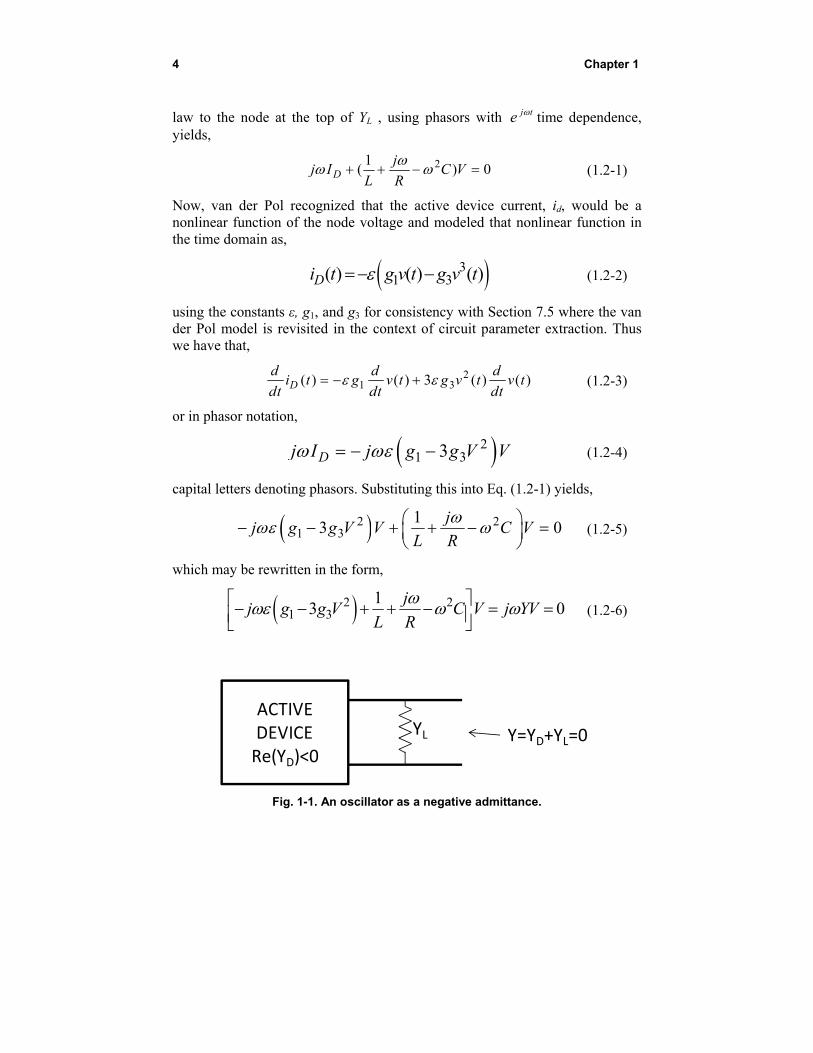
Fig. 1-1. An oscillator as a negative admittance.
ACTIVE DEVICERe(YD)<0
YL Y=YD+YL=0
Introduction 5
where,
21 3
1 13Y g g V j C
j L R
(1.2-7)
Now, expanding this admittance in a Taylor series about the resonant frequency,
01
LC (1.2-8)
results in,
21 3
21 3 0
0
1 13
23
Y g g V j Cj L R
jQg g V
R
(1.2-9)
where,
0Q RC (1.2-10)
is the traditional quality factor of the oscillator. Use of this expression for the admittance is how we will introduce the van der Pol model into our analysis of an injection locked oscillator below.
1.3 Injection Locking (Adler’s Formalism) and Its Spectra (Locked and Unlocked)
To analytically describe the injection locking phenomenon, an oscillator can be viewed as an admittance with a negative real part connected to a resonant load admittance with a positive real part as shown in Fig. 1-1. Using this representation we proceed now to develop a differential equation for the dynamic behavior of the phase of the oscillation. The voltage across the load admittance can be written in time varying phasor form as,
6 Chapter 1
( )( ) j tV A t e (1.3-1)
where,
0( ) ( )t t t (1.3-2)
Note that V may also be written,
[ ( ) ln ( )]j t j A tV e (1.3-3)
Kurokawa [15] suggested that the time derivative of this phasor be written in the form,
0 lndV d d
j j A Vdt dt dt
(1.3-4)
and that the quantity in brackets be identified as the “instantaneous frequency,”
inst . That is,
instdV
j Vdt
(1.3-5)
where,
0 lninstd d
j Adt dt
(1.3-6)
The negative admittance of the device, YD, is a function of both the frequency and the amplitude of the oscillating voltage across it. The oscillator operates at the frequency and amplitude that makes this negative admittance equal to the negative of the load admittance, YL, so that the total admittance is zero. Following Chang, Shapiro, and York [16], we may expand the admittance in a Taylor series about this operating point in the form,
0
0 0 0( , ) ( , ) ( )inst L D instY
Y A Y Y A
(1.3-7)
where we have neglected the amplitude dependence of YD. Multiplying by V we obtain Kirchhoff’s current law at the top node of Fig. 1-1.
Introduction 7
0
0 0 0
( , )
( , ) ( ) 0
inst
L D inst
Y A V
YY V Y A V V
(1.3-8)
In steady state, the oscillator will oscillate with frequency ω0 and amplitude A0 making the derivative term zero. Then the load current cancels the oscillator current for a total of zero current exiting the node. However, if a signal is injected at the node from an external source, this equilibrium is changed to,
0
0 0 0
( , )
( , ) ( ) 0
inj inst
inj L D inst
I Y A V
YI Y V Y A V V
(1.3-9)
Inserting Eq. (1.3-6) for the instantaneous frequency results in,
0
0 0( , ) ln 0inj D Ld d Y
I Y A V Y V j A Vdt dt
(1.3-10)
or,
0 0
0 0( , )ln 0injIY Ad d
j AY Ydt dt
V
(1.3-11)
We will now substitute the negative admittance appropriate to the van der Pol oscillator model and analyze the oscillator assuming that a current, Iinj, is injected. Recall that near ω0 van der Pol’s model gives,
21 3 0
0
23
osc
jQY g g V
R
(1.3-12)
so that,
0 0
2
osc
Y jQ
R
(1.3-13)
Taking the real part of (1.3-11) using (1.3-13) yields,
8 Chapter 1
0
Re 02
inj
osc
IdjQdt VR
(1.3-14)
Letting inj osc injV R I ,
0 Im 02
injVd
dt Q V
(1.3-15)
Using phasor notation for the injection signal, injjinj injV A e
and using
(1.3-2),
0 0
0 0Im sin2 2
injjinj injinj
A Ade
dt Q A Q A
(1.3-16)
Defining, 0
2inj
lock
A
Q A
, the so-called “locking range,” we have,
0 sinlock injd
dt
(1.3-17)
known as Adler’s equation [10]. Taking the imaginary part of Eq. (1.3-11) leads in the same manner to a differential equation for the amplitude dynamics but, treatment of that aspect will be postponed until Chapter 7 dealing with nonlinear analysis of oscillator arrays. For clarity and simplicity in the initial description of the array properties, the amplitude variation will be assumed negligible. If you are particularly interested, however, you may wish to consult Nogi, et al. [17], Meadows, et al. [18] , and Seetharam, et al. [19] which discuss some aspects of amplitude behavior. Although the differential equation given by Eq. (1.3-17) is first order, it is nonlinear. Remarkably, however, it can nevertheless be solved analytically. Once the solution is obtained, it can be used to describe the dynamic behavior of the locking process and, very interestingly, the spectrum of the oscillations under both locked and unlocked conditions. We begin by solving Eq. (1.3-17) and then proceed to exhibit the spectral properties of the solution. First, we define,
Introduction 9
0inj inj inj t (1.3-18)
so that Eq. (1.3-17) may be written,
sin injlock
lock
d
dt
(1.3-19)
where 0inj inj . Now defining inj
lockK
and lockt , we
have the deceptively simple looking differential equation,
sind
Kd
(1.3-20)
Integrating from an initial time, 0 , to an arbitrary subsequent time, ,
0 0
( )
( ) sin
dd
K
(1.3-21)
we arrive at,
0
( )0 ( ) sin
d
K
(1.3-22)
and it remains to carry out the integration. Using the substitution,
tan2
u
(1.3-23)
the integral may be cast in the form,
0 2
1 22
1
u
u
duuK u
K
(1.3-24)
where,
00
( )tan
2u
(1.3-25)
10 Chapter 1
By factoring the denominator of the integrand and expanding in partial fractions, the integral, Eq. (1.3-24), can be expressed in terms of the natural logarithm function in the form,
0
0
2
22 1
1 2 1ln
2 11
uu
uu
u uduuK u uKu
K
(1.3-26)
where u1 and u2 are the roots of the quadratic in the denominator of the integrand. That is, Eq. (1.3-22) becomes,
0
0
( )
( )
( )2
02 2
( )
sin
tan 1 11 2
ln1 tan 1 1
2
d
K
K K
K K K
(1.3-27)
Recall that the natural logarithm function is related to the inverse hyperbolic tangent function by,
11ln 2 tanh
1
xx
x
(1.3-28)
if 10 2 x . Upon using Eq. (1.3-28) in Eq. (1.3-27) we obtain,
0
( )
21
0 2
( )
2 1tanh
1 tan 12
K
K K
(1.3-29)
provided 2 1K . This condition is equivalent to,
inj lock (1.3-30)
which means that the injection signal frequency is within one locking range of the free-running frequency of the oscillator corresponding to the so-called

Introduction 11
“locked” condition. If 2 1K , the oscillator is said to be “unlocked” and the solution given by Eq. (1.3-27) becomes,
0
( )
21
0 2
( )
2 1tan
1 tan 12
K
K K
(1.3-31)
Now, rewriting Eqs. (1.3-29) and (1.3-31) explicitly evaluated at the limits and rearranging a bit results in,
20
2 21 1
0
11
2
1 1tanh tanh
( ) ( )tan 1 tan 1
2 2
K
K K
K K
(1.3-32)
and,
20
2 21 1
0
11
2
1 1tan tan
( ) ( )tan 1 tan 1
2 2
K
K K
K K
(1.3-33)
We now make use of the following pair of identities.
1 1 1 00
0
tanh ( ) tanh ( ) tanh1
x xx x
xx
(1.3-34)
1 1 1 0
00
tan ( ) tan ( ) tan1
x xx x
xx
(1.3-35)
Applying these to Eqs. (1.3-32) and (1.3-33), respectively, we obtain,
12 Chapter 1
20
0
0 0
1tanh 1
2
( )( )tan tan
2 2
( ) ( )( ) ( )tan tan tan tan
2 2 2 2
K
K K
(1.3-36)
20
0
0 0
1tan 1
2
( )( )tan tan
2 2
( ) ( )( ) ( )tan tan tan tan
2 2 2 2
K
K K
(1.3-37)
These equations may now be solved for ( ) . The results are,
20 00
1
2 00
( )
( ) ( )1tan tanh 1 tan
2 2 22tan
( )11 tanh 1 1 tan
2 2
K K
K K
(1.3-38)
20 00
1
2 00
( )
( ) ( )1tan tan 1 tan
2 2 22tan
( )11 tan 1 1 tan
2 2
K K
K K
(1.3-39)
These represent the exact analytic solution of Eq. (1.3-20) giving the dynamic behavior of the phase of an externally injection locked oscillator for all time
subsequent to 0 . While they are actually the same solution, Eq. (1.3-38) is
Introduction 13
conveniently applied when 2 1K , and Eq. (1.3-39) is conveniently applied
when 2 1K . When 12 K , Eqs. (1.3-38) and (1.3-39) are identical. We will now proceed to study the spectral properties of this solution. It will be expedient to return to the logarithmic representation in Eq. (1.3-27). For the locked condition we have,
22 0
2 20
20
( )( )tan 1 1tan 1 1
22ln
( ) ( )tan 1 1 tan 1 1
2 2
1
K KK K
K K K K
K
(1.3-40)
Exponentiating both sides yields,
20
22 0
2 20
1
( )( )tan 1 1tan 1 1
22( ) ( )
tan 1 1 tan 1 12 2
K
K KK K
K K K K
e
(1.3-41)
For simplicity of notation, the second factor in the curly brackets, being a constant that depends on the initial conditions, will be defined to be 1/C0. Thus,
20
2
10
2
( )tan 1 1
2( )
tan 1 12
KK K
C eK K
(1.3-42)
Now solving for ( ) ,
20
20
121 0
10
11 1( ) 2tan
1
K
K
C eK
K KC e
(1.3-43)
Recall that,
14 Chapter 1
1tan ( ) ln
2
j j xx
j x
(1.3-44)
So that Eq. (1.3-43) may be written in the form,
20
20
20
20
120
10
120
10
11 1
1( ) ln
11 1
1
K
K
K
K
C eKj
K KC ej
C eKj
K KC e
(1.3-45)
Again exponentiating both sides,
20
20
20
20
120
10( )
120
10
11 1
1
11 1
1
K
Kj
K
K
C eKj
K KC ee
C eKj
K KC e
(1.3-46)
This can be rearranged as,
20
20
( )
12 20
12 20
1 1 1 1
1 1 1 1
j
K
K
e
jK K jK K C e
jK K jK K C e
(1.3-47)
Equation (1.3-47) gives the dynamic behavior of the oscillator voltage as the phase evolves from )( 0 to )( . This behavior is exponential, not
oscillatory, and the steady-state value of the phase at infinite time is
)(sin 1 K . Returning to Eq. (1.3-1) and using Eq. (1.3-18) we find that the oscillator voltage in steady state is,
1( ) ( sin ( )( )( ) inj inj injj j K tj tssV A t e Ae Ae
(1.3-48)
Introduction 15
Thus, the spectrum is a single line at frequency inj and there is a steady-state
phase difference between the oscillator signal and the injection signal of
)(sin 1 K . Suppose we allow K to become larger than unity in magnitude. In such a case, the injection signal frequency lies outside the locking range around the free running frequency and the oscillator will be in the “unlocked” condition described by Eq. (1.3-39). Now, however, the spectral properties of the solution become more interesting. We follow an approach suggested by Armand. [20] In this situation, Eq. (1.3-47) becomes,
20
20
( )
12 20
12 20
1 1 1 1
1 1 1 1
j
j K
j K
e
jK j K jK j K C e
jK j K jK j K C e
(1.3-49)
or,
( ) 1 2 0
1 2 0
jTj
jT
A A C ee
B B C e
(1.3-50)
where,
21
22
21
22
1 1
1 1
1 1
1 1
A jK j K
A jK j K
B jK j K
B jK j K
(1.3-51)
201T K (1.3-52)
and,
16 Chapter 1
20
020
( )tan 1 1
2( )
tan 1 12
K j KC
K j K
(1.3-53)
Expanding Eq. (1.3-49) in a geometric series yields,
( ) 1 1 2 20
1 1 2 11
nj jnT
n
A A A Be C e
B B B B
(1.3-54)
Now, the magnitude of the common ratio of the series is,
20
1
202
2 20
22
22
( )tan 1 1
1 1 2( )1 1 tan 1 12
1 1
1 1
BC
B
K j KjK j K
jK j K K j K
K K
K K
(1.3-55)
This is less than unity for positive K and the series converges for all T. If, on the other hand, K is negative, we instead expand the reciprocal of Eq. (1.3-49),
( ) 1 2 0
1 2 0
1 1 2 20
1 1 2 11
jTj
jT
njnT
n
B B C ee
A A C e
B B B AC e
A A A A
(1.3-56)
and the magnitude of the common ratio is,
Introduction 17
20
1
202
2 20
22
22
( )tan 1 1
1 1 2( )1 1 tan 1 12
1 1
1 1
AC
A
K j KjK j K
jK j K K j K
K K
K K
(1.3-57)
which is less than unity for K negative. Expressions (1.3-54) and (1.3-56) thus provide convergent series representations of the solution for the phase dynamics under unlocked conditions and we note that they are actually Fourier series. As such, the coefficients are the amplitudes of the harmonics of a line spectrum representing the oscillator signal. This spectrum has a well-known classic form that is easily observed experimentally using a spectrum analyzer and is depicted schematically in Fig. 1-2.
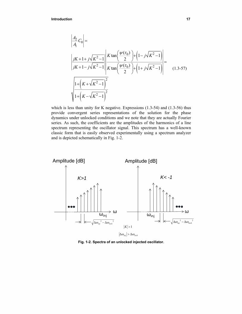
Fig. 1-2. Spectra of an unlocked injected oscillator.
Amplitude [dB]
ωωinjω
ωinj
Amplitude [dB]
K>1 K< -1
1K
lockinj
22lockinj
22lockinj
18 Chapter 1
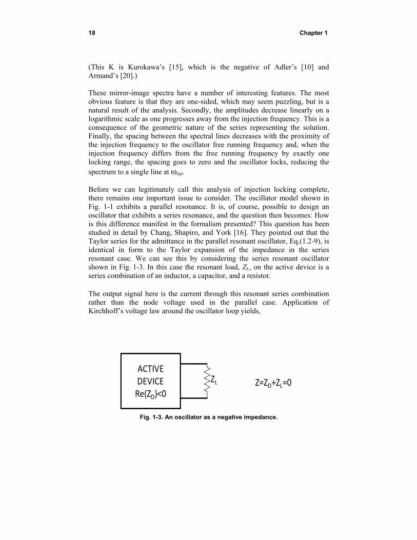
(This K is Kurokawa’s [15], which is the negative of Adler’s [10] and Armand’s [20].) These mirror-image spectra have a number of interesting features. The most obvious feature is that they are one-sided, which may seem puzzling, but is a natural result of the analysis. Secondly, the amplitudes decrease linearly on a logarithmic scale as one progresses away from the injection frequency. This is a consequence of the geometric nature of the series representing the solution. Finally, the spacing between the spectral lines decreases with the proximity of the injection frequency to the oscillator free running frequency and, when the injection frequency differs from the free running frequency by exactly one locking range, the spacing goes to zero and the oscillator locks, reducing the spectrum to a single line at ωinj. Before we can legitimately call this analysis of injection locking complete, there remains one important issue to consider. The oscillator model shown in Fig. 1-1 exhibits a parallel resonance. It is, of course, possible to design an oscillator that exhibits a series resonance, and the question then becomes: How is this difference manifest in the formalism presented? This question has been studied in detail by Chang, Shapiro, and York [16]. They pointed out that the Taylor series for the admittance in the parallel resonant oscillator, Eq.(1.2-9), is identical in form to the Taylor expansion of the impedance in the series resonant case. We can see this by considering the series resonant oscillator shown in Fig. 1-3. In this case the resonant load, ZL, on the active device is a series combination of an inductor, a capacitor, and a resistor. The output signal here is the current through this resonant series combination rather than the node voltage used in the parallel case. Application of Kirchhoff’s voltage law around the oscillator loop yields,
Fig. 1-3. An oscillator as a negative impedance.
ACTIVE DEVICERe(ZD)<0
ZL Z=ZD+ZL=0
Introduction 19
1
( ) 0DV j L R Ij C
(1.3-58)
Using a van der Pol type nonlinearity, the analog of Eq. (1.2-2) is,
31 3( ) ( ) ( )Dv t ri t r i t (1.3-59)
and the analog of Eq. (1.2-7) is,
21 3
1 13Z r r I j L R
j C Y
(1.3-60)
Expanding Y in a Taylor series about the resonant frequency, we arrive at
0201 3
1 2
3
jQY
RR r r I
(1.3-61)
Comparing with Eq. (1.2-9) we see that the salient difference is the change in sign of the linear term in frequency. This in turn induces a change in the algebraic sign of the sine term in Eq. (1.3-17) resulting in,
0 sinlock injd
dt
(1.3-62)
and the remainder of the analysis proceeds as for the parallel resonant case above. We will further describe the implications of this when we consider more than one oscillator.
1.4 Mutual Injection Locking of Two Oscillators
Consider now two parallel resonant oscillators, identical except for free-running frequency, coupled together so that each injects a signal into the other. Such a system was considered by Stephan and Young [3] in which the coupling was due to free-space mutual coupling between radiating elements excited by the oscillators. We may describe this situation using Adler’s Eq. (1.3-17) for each oscillator. That is,
101 2 1sinlock
d
dt
(1.4-1)
20 Chapter 1
202 1 2sinlock
d
dt
(1.4-2)
where the subscripts identify the oscillators. Subtracting these equations yields,
1 2
01 02 2 12 sinlockd
dt
(1.4-3)
We now define,
1 2 (1.4-4)
02 01
2 lock
K
(1.4-5)
2 lockt (1.4-6)
so that Eq. (1.4-3) becomes,
sind
Kd
(1.4-7)
which is identical with Eq. (1.3-20) except for the tildes and all of the preceding results apply. Note that the locking range is replaced by twice the locking range in this equation. This happens because the injecting oscillator frequency is permitted to change under the influence of the oscillator being injected. The result is that the two oscillator frequencies can differ by nearly twice the locking range and still maintain lock. This is true because it will turn out that the steady-state oscillation frequency of the pair is the average of the two free-running frequencies, and we can show this as follows.
Recall that in steady state, if 1~ K so the oscillators are locked,
1sin K , a constant, so its time derivative is zero. Further, from Eq. (1.4-4) we have,
1 2 (1.4-8)
so that, in steady state,
Introduction 21
1 2 2d d dd
d d d d
(1.4-9)
Therefore,
1 2 12d d d
d d d
(1.4-10)
or,
01 021 1 2
2 2
d d
d d
(1.4-11)
Similarly,
01 022 1 2
2 2
d d
d d
(1.4-12)
Thus, we conclude that the steady-state frequency of the two oscillators, when mutually locked, that is, the “ensemble frequency,” is the average of their free-running frequencies. It now becomes clear how it is that the locking range for the two oscillators is twice that for one. One may visualize each oscillator differing from the ensemble frequency of the pair by one locking range so that the total difference between the free-running frequencies of the two oscillators is, not one, but two locking ranges. The term “ensemble frequency” has no relevance when one of the oscillators injection locks the other and is not influenced by the injected oscillator as discussed previously. In that case, as was demonstrated, the steady-state frequency is the injection frequency. Now suppose that the coupling between the oscillators is accomplished via a transmission line so that there is a phase delay associated with the coupled signal. This coupling phase changes the phase relationship between the coupled signal and the oscillator that produced it and thus modifies the behavior of the oscillator pair. We can account for this in our formulation by inserting the coupling phase shift through the transmission line, 12 , into Eqs. (1.4-1) and (1.4-2) resulting in,
101 2 1 12sinlock
d
dt
(1.4-13)
22 Chapter 1
202 1 2 12sinlock
d
dt
(1.4-14)
where we have assumed that the transmission line is reciprocal so that the coupling phase is the same in both directions. Using trigonometric identities, Eqs. (1.4-13) and (1.4-14) may be re-written in the form,
101 12 2 1
12 2 1
sin cos
cos sin
lock
lock
d
dt
(1.4-15)
202 12 1 2
12 1 2
sin cos
cos sin
lock
lock
d
dt
(1.4-16)
Again by subtraction we obtain,
1 2
01 02 12 1 22 cos sinlockd
dt
(1.4-17)
Comparing with Eq. (1.4-3) we see that the locking range has been modified by the cosine of the coupling phase. We define this effective locking range to be,
12coseff lock (1.4-18)
and using this in place of the unmodified locking range, the preceding theory may be applied to the case having non-zero coupling phase. One obvious consequence of this is that, if the coupling phase is 90 degrees (deg) or an odd multiple thereof, the effective locking range becomes zero and the two oscillators cannot be made to lock. If, instead of subtracting Eqs. (1.3-15) and (1.3-16), we add them, we obtain
1 2
01 02 12 1 22 sin coslockd
dt
(1.4-19)
and we note that the ensemble frequency Eq. (1.4-12) is replaced by,
01 02
12 1 2sin cos( )2ens lock
(1.4-20)
which varies sinusoidally with coupling phase. This variation of ensemble frequency with coupling phase has been studied in somewhat more detail by
Introduction 23
Sancheti and Fusco in the context of an active radiator coupling with its image in a reflecting object [21] [22]. Before moving on to study arrays of oscillators we take a quick look at the stability of the behavior of two coupled oscillators. Much more detail on this subject may be found in Chapter 7. The stability of the solution can be assessed by assuming that the oscillators are evolving according to a solution of Eq. (1.4-17) and perturbing the phase difference away from that solution by a small amount, . This results in the following differential equation for the time dependence of the perturbation.
12 1 22 cos coslockd
dt
(1.4-21)
This equation has the solution,
12 1 22 cos cos( ) lock tt e
(1.4-22)
The solution for the oscillator phase difference is stable against the perturbation, δ, if the exponent is negative. That is,
12 1 2cos cos 0 (1.4-23)
This means that, if the magnitude of the coupling phase is less than 90 deg, the oscillators will lock such that their phases differ by less than 90 deg; while if the magnitude of the coupling phase is greater than 90 deg, the oscillators will lock such that their phases differ by more than 90 deg; that is, they will tend to oscillate out of phase. This behavior was predicted and observed by Stephan and Young [3] and formulated and studied in more detail by Humphrey and Fusco [23] [24] using an earlier theoretical construct they formulated for linear chains of coupled oscillators [25]. Conversely, for series resonant oscillators, the stability condition is,
12 1 2cos cos 0 (1.4-24)
and the behavior of the oscillators will be opposite that described above. These properties have been exploited by Lee and Dalman in switching pairs of coupled oscillators from symmetric to antisymmetric phase by changing the coupling phase [26]. All of these effects have been observed experimentally as reported by Chang, Shapiro, and York [16]. Thus, the optimum coupling phase
24 Chapter 1
for parallel resonant oscillators is an even multiple of 180 deg, while that for series resonant oscillators is an odd multiple of 180 deg. Very recently, it was pointed out that a given oscillator can present either series or parallel resonance depending upon where in the oscillator circuit the coupling is implemented [27].
1.5 Conclusion
In this Chapter we have developed a theory of oscillator behavior that admits the possibility of coupling the oscillators together such that they can mutually injection lock and thus oscillate as a coherent ensemble. This behavior is central to the remainder of the book as it forms the basis of the applications to be discussed. In Chapter 2 this theoretical framework will be applied in describing the behavior of arrays containing many oscillators coupled together in linear and planar configurations. The coupling for the most part is with nearest neighbors only. More elaborate coupling schemes have been studied in mathematical biology but remain as a potentially fruitful but largely untapped resource in the arena of phased-array antennas.
25
Chapter 2
Coupled Oscillator Arrays – Basic Analytical Description and Operating
Principles
In this chaper we will show how to use the theory developed in Chapter 1 to mathematically describe a linear array of oscillators coupled to nearest neighbors. It was Karl Stephan who first showed that such arrays can be useful in providing excitation signals for a linear array of radiating elements in that if locking signals are injected into the end oscillators of the array, variation of the relative phase of the locking signals can be used to control the distribution of the phase of the signals across the array [1]. Later, Liao and York pointed out that by merely tuning the end oscillators of the array the phase distribution can be controlled without any external injection signals [28]. We will show that, while the equations and associated boundary conditions at the array ends can describe the nonlinear behavior of the array through numerical solution, if the inter-oscillator phase differences remain small, the equations may be linearized. The linearized version may be solved analytically for the dynamic behavior of the phase, and from this one may obtain the dynamic behavior of the beam radiated by the elements of this linear phased array antenna. An important consideration in the analysis is the manner in which the oscillators are coupled. The coupling can be represented as a “coupling network” connected to the array of oscillators, and this network can be
26
described in matrix or its The above thoscillators cosolution of thterms of port
2.1 Fund
Recall that tdescribed by2N+1 oscilla(1.4-2) is,
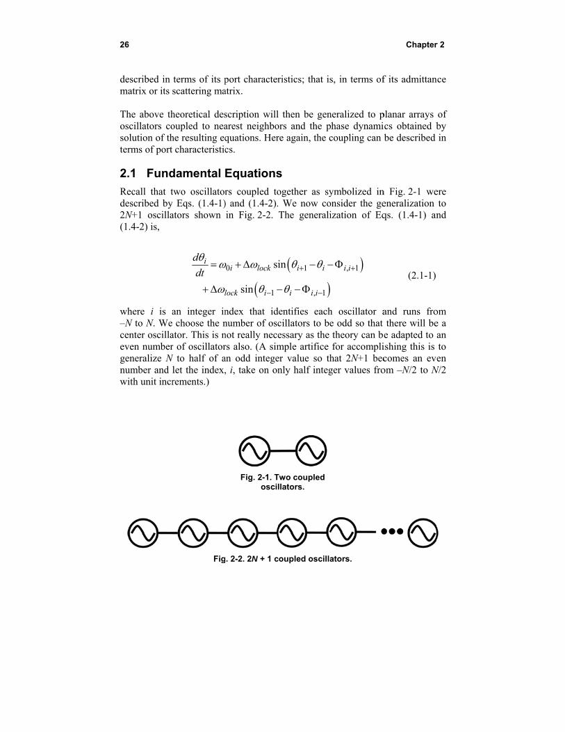
where i is a–N to N. Wecenter oscillaeven numbergeneralize Nnumber and with unit incr
terms of its pscattering ma
heoretical desoupled to neahe resulting eqt characteristic
damental
two oscillatory Eqs. (1.4-1)ators shown
i
l
d
dt
an integer in choose the n
ator. This is nr of oscillator
N to half of alet the index,rements.)
Fig
port characteratrix.
scription willarest neighboquations. Hercs.
Equations
rs coupled to) and (1.4-2).in Fig. 2-2.
0
1
si
sin
i lock
lock i
ndex that idnumber of oscnot really necers also. (A siman odd intege, i, take on on
Fig. 2-1. Tosci
g. 2-2. 2N + 1 c
ristics; that is
l then be genors and the pre again, the c
s
ogether as sy. We now coThe generali
1
, 1
in i i
i i i
dentifies eachcillators to beessary as the mple artifice er value so thnly half integ
Two coupled llators.
coupled oscilla
s, in terms of
neralized to pphase dynamicoupling can
ymbolized inonsider the geization of Eq
, 1i i
h oscillator ae odd so that theory can bfor accompli
hat 2N+1 becger values fro
ators.
Chapter
f its admittan
planar arrays ics obtained bbe described
n Fig. 2-1 weeneralization qs. (1.4-1) an
(2.1-1)
and runs frothere will be
e adapted to ishing this is comes an evom –N/2 to N
r 2
nce
of by in
ere to nd
om e a an to en
N/2
COAs—Basic Analytical Description and Operating Principles 27
However, from a practical point of view, it is convenient to have a center point at which to inject an external signal from a stable oscillator for the purpose of stabilizing the array oscillation. We therefore select the number to be odd. Note that, because the end oscillators are coupled to only one other oscillator, they are described by differential equations with only one sine term on the right side; that is,
0 1 , 1sinNN lock N N N N
d
dt
(2.1-2)
0 1 , 1sinNN lock N N N N
d
dt
(2.1-3)
Note further that, because the maximum magnitude of the sine function is unity, the end oscillators of the array can be detuned from their nearest neighbors by a maximum of one locking range without losing lock whereas the center oscillator can be detuned up to two locking ranges. The maximum permitted detuning of the other oscillators will lie between one and two locking ranges. (See Section 3.1, Eq. (3.1-35).) This system of simultaneous nonlinear first-order differential equations, (2.1-1)—(2.1-3), can be solved numerically beginning with an initial phase distribution and oscillator tuning thus providing the phase distribution at all subsequent times. However, numerical solution does not provide an intuitive grasp of the behavior and how the parameters affect it. This intuitive understanding may be more easily gleaned from an approximate analytic solution. Then, later, if a more exact result is needed, the numerical approach can be applied. Before proceeding to solve Eqs. (2.1-1) to (2.1-3) by linearization, we remark that the oscillator tuning required to produce a desired steady-state phase distribution may be easily obtained from these equations. That is, in steady state the time derivatives are zero, and from (2.1-1) to (2.1-3) the oscillator tuning is merely,
0 1 , 1
1 , 1
sin
sin
i ref lock i i i i
lock i i i i
(2.1-4)
0, 1 , 1sinN ref lock N N N N (2.1-5)
28 Chapter 2
0 1 , 1sinN ref lock N N N N (2.1-6)
where we have defined a new phase variable via,
i i ref t (2.1-7)
and ref is taken to be the ensemble frequency of the array.
Let us assume for the moment that the coupling phases are a multiple of π, and sum (2.1-4)–(2.1-6) over the 2N+1 array elements. We find that under this assumption,
0
1
1 11
1 1
sin sin
sin sin 0
N
i refi N
N
lock i i i ii N
lock N N lock N N
N
(2.1-8)
so that,
01 N
ref ii NN
(2.1-9)
the average of the free-running frequencies. Thus, we have shown that for coupling phase equal to a multiple of π, the ensemble frequency of the array is the average of the free running frequencies of the oscillators. As an example, in an array with zero coupling phase, a linear phase distribution with an inter-oscillator phase difference of requires,
0 0i ref (2.1-10)
0, sinN ref lock (2.1-11)
0 sinN ref lock (2.1-12)
COAs—Basic Analytical Description and Operating Principles 29
Thus, beginning with all the oscillators tuned to the reference frequency, tuning the leftmost oscillator down in frequency by half of the locking range and tuning the rightmost oscillator up in frequency by half of the locking range will produce a phase distribution across the array with a positive slope of π/6 radians between oscillators, π/6 being the arcsine of 1/2. If the oscillator outputs are used to excite radiating elements spaced a half wavelength (π radians) apart, the radiated beam will be directed 9.6 deg from normal to the array, that is, the arcsine of 1/6. It is this method of beam-steering that was first described by Liao and York. [28] Of course, much more general phase distributions are possible and the required oscillator tunings to produce them are given by Eqs. (2.1-4)–(2.1-6).
2.2 Discrete Model Solution (Linearization and Laplace Transformation)
In order to render the analytic solution tractable, we assume that the arguments of the sine functions in Eqs. (2.1-1)–(2.1-2) are close to an integral multiple of 2π. Specifically, we will assume that the coupling phase is zero and that the inter-oscillator phase differences are small so that the sine functions can be approximated by their arguments. In this approximation, Eq. (2.1-1) becomes,
0 1 12ii lock i i i
d
dt
(2.2-1)
Similarly, Eqs. (2.1-2) and (2.1-3) become,
0, 1N
N lock N Nd
dt
(2.2-2)
0 1N
N lock N Nd
dt
(2.2-3)
Note that these approximate linearized equations would seem to imply that the end oscillators of the array can be detuned by π/2 locking ranges and the center
one can be detuned by π locking ranges and still remain locked because the phase differences between oscillators remain less than or equal to π/2. However, from the full nonlinear theory of Section 2.1, we know that this is actually not true. These linearized equations only apply when the phase differences are small so that the sine functions may be accurately replaced by their arguments and π/2 is certainly not a small value in this sense. In terms of the new phase, Eq. (2.1-7), we find that Eqs. (2.2-1)–(2.2-3) become,
30 Chapter 2
0 1 12ii ref lock i i i
d
dt
(2.2-4)
0, 1N
N ref lock N Nd
dt
(2.2-5)
0 1N
N ref lock N Nd
dt
(2.2-6)
Now we have a system of first-order linear differential equations that describe the dynamic behavior of the oscillator array. Unlike the system of first-order nonlinear differential equations from which it was derived, this system can be solved analytically. We begin by writing these linear equations, Eqs. (2.2-4)–(2.2-6), in matrix form,
0[ ]
[ ] [ ] [ ][ ]ref lockd
Mdt
(2.2-7)
where [ ] is a 2N+1 element vector of oscillator phases, [ω0] is a similar vector of oscillator free-running frequencies, and [M] is a (2N+1) by (2N+1) tridiagonal matrix with –2’s on the diagonal, except for the –1’s in the upper left and lower right corners, and 1’s on the first super and sub diagonals.
Dividing by lock yields,
[ ]
[ ] [ ][ ]tuned
Md
(2.2-8)
where lockt and 0[ ] i reftune
lock
, a vector of oscillator free
running frequencies relative to the reference frequency (detuning frequencies). Laplace transformation with respect to gives,
[ [ ] [ ]][ ] [ ]tunes I M (2.2-9)
with the tildes indicating transformed quantities and with [I] being the identity matrix. We now define eigenvectors, [v]n , and eigenvalues, λn , of the matrix [M] to be such that,
[ ]][ ] [ ]n n nM v v (2.2-10)
COAs—Basic Analytical Description and Operating Principles 31
Our intention is to express the solution of Eq. (2.2-9) as a sum of these eigenvectors with unknown coefficients. When this sum is substituted into Eq. (2.2-9), the orthogonality of the eigenvectors will be employed to determine the coefficients of the expansion and thus obtain the solution in series form. Since the number of eigenvectors is finite, this series will be a finite sum; that is, a closed form. Moreover, as we will see in the next section, in steady state, an approximation of this sum may be carried out to produce a simple functional form for the phase distribution. Note that Eq. (2.2-10) is a three term recurrence relation for the elements of the
eigenvectors, iv ; that is,
1 1(2 ) 0i n i iv v v (2.2-11)
with the two auxiliary conditions,
1 (1 ) 0N n Nv v (2.2-12)
1 (1 ) 0N n Nv v (2.2-13)
Now, Eq. (2.2-11) is satisfied by the Chebyshev polynomials, ( )i nT x and
( )i nU x , where,
2
2n
nx
(2.2-14)
so that Eqs. (2.2-12) and (2.2-13) become,
1( ) (2 1) ( ) 0N n n N nW x x W x (2.2-15)
1( ) (2 1) ( ) 0N n n N nW x x W x (2.2-16)
where Wi is a linear combination of Ti and Ui-1. Equivalently, using (2.2-11) we have,
1( ) ( ) 0N n N nW x W x (2.2-17)
1( ) ( ) 0N n N nW x W x (2.2-18)
These boundary condition equations determine the permissible values, xn. Let
32 Chapter 2
1( ) ( ) ( )i n T i n U i nW x T x U x (2.2-19)
so that
1( ) ( ) ( )i n T i n U i nW x T x U x (2.2-20)
Adding and subtracting Eqs. (2.2-17) and (2.2-18) using Eqs. (2.2-19) and (2.2-20) yields,
1( ) ( ) 0N n N nT x T x (2.2-21)
1( ) ( ) 0N n N nU x U x (2.2-22)
Using the trigonometric expression for T, Eq. (2.2-21) yields,
1 11 1
sin cos ( ) sin cos ( ) 02 2n nN x x
(2.2-23)
which implies that,
2
cos(2 1)T n
nx
N
(2.2-24)
so that the eigenvalues are given by,
222 cos 2 4 sin
(2 1) (2 1)Tnn n
N N
(2.2-25)
the subscript T indicating that the elements of the corresponding eigenvectors
are ( )i nT x . Conversely, using the trigonometric expression for U, Eq. (2.2-22)
yields,
11
cos cos ( ) 02 nN x
(2.2-26)
which implies that,
2 1
cos2 1Unn
xN
(2.2-27)
so that the eigenvalues are given by,
COAs—Basic Analytical Description and Operating Principles 33
22 1 2 1 / 22cos 2 4sin
2 1 2 1Unn n
N N
(2.2-28)
the subscript U indicating that the elements of the corresponding eigenvectors
are 1( )i nU x . In (2.2-25) and (2.2-28) the index n runs from 0 to N after which
the eigenvalues repeat. Thus, we have arrived at two sets of eigenfunctions, one set, the T’s, excited by the symmetric part of the detuning function and the other set, the U’s, excited by the antisymmetric part, with respect to the array center. We may now expand the solution of Eq. (2.2-9) in these eigenvectors as,
0
[ ] [ ] [ ]N
n T n n U nn
A v B v
(2.2-29)
Substituting this expansion into Eq. (2.2-9), we obtain,
0
0
[ [ ] [ ]] [ ] [ ]
( )[ ] ( )[ ] [ ]
N
n T n n U nn
N
n Tn T n n Un U n tunen
s I M A v B v
A s v B s v
(2.2-30)
Using the orthogonality of the eigenvectors, we may now solve for the coefficients An and Bn.
[ ] [ ]
( )[ ] [ ]tune T n
nTn T n T n
vA
s v v
(2.2-31)
[ ] [ ]
( )[ ] [ ]tune U n
nUn U n U n
vB
s v v
(2.2-32)
Substituting into Eq. (2.2-29),
34 Chapter 2
0
0
[ ] [ ][ ] [ ]
( )[ ] [ ]
[ ] [ ][ ]
( )[ ] [ ]
Ntune T n
T nTn T n T nn
Ntune U n
U nUn U n U nn
vv
s v v
vv
s v v
(2.2-33)
and, if the detuning function is a step function at time zero, the inverse Laplace transform is,
,
1
0
[ ]2 1
[ ] [ ][ ] 1
[ ] [ ]
[ ] [ ][ ] 1
[ ] [ ]
Tn
U n
N
tune ii N
Ntune T n
T nTn T n T nn
Ntune U n
U nUn U n U nn
N
vv e
v v
vv e
v v
(2.2-34)
The first of the three summations, the one arising from the zero eigenvalue, indicates that the steady-state ensemble frequency of the array is shifted by the average oscillator detuning; i.e., the sum of the elements of the tunevector divided by the number of oscillators. Recall that we assumed at the start of this section that the coupling phase is zero. Returning for a moment to Eq. (2.1-1) and using Eq. (2.1-7), we may write,
0 1 , 1
1 , 1
sin
sin
ii ref lock i i i i
lock i i i i
d
dt
(2.2-35)
If the coupling phases are taken to be equal, this can be rearranged to read,
0 1 1
1 1
sin cos cos
cos sin sin
ii ref lock i i i i
lock i i i i
d
dt
(2.2-36)
or,
COAs—Basic Analytical Description and Operating Principles 35
0 1 1sin sinii ref eff i i i i
d
dt
(2.2-37)
where,
1 1sin cos cosref ref lock i i i i (2.2-38)
and
coseff lock (2.2-39)
which is the same as Eq. (1.4-18). Thus we conclude that, in a 2N+1 oscillator array, a uniform coupling phase modifies the effective locking range according to Eq. (2.2-39) just as it did for two oscillators, and the ensemble frequency is modified according to Eq. (2.2-38). Interestingly, if the inter-oscillator phase difference is 90 deg, the ensemble frequency becomes independent of the coupling phase as pointed out by Humphrey and Fusco [25]. The speed of the array response to the application of a step tuning is determined by the smallest nonzero eigenvalue. From Eq. (2.2-28) this is,
22
0/ 2
4sin(2 1) (2 1)U N N
(2.2-40)
This provides the important result that the linear array response time constant is roughly proportional to the square of the number of elements, the approximation becoming more accurate as the number of elements is increased. While the time constant is unaffected, the effective steering speed of such arrays, as defined by the radiated beam peak neglecting aberration, may be increased by “over-steering.” That is, one may apply more detuning than necessary to achieve the desired steady-state phase gradient but reduce it to the required value during the beam-steering transient. Generalizing this concept, one may apply arbitrarily time-varying detuning as suggested by Heath et al. [29]. In particular they considered sinusoidal detuning and showed that the maximum stable inter-oscillator phase shift is thereby increased from 90 to 138 deg.
2.3 Steady-State Solution
In this section we will investigate the steady-state solution for the phase distribution in a bit more detail. From Eq. (2.2-34), the steady-state solution is,
36 Chapter 2
1
0
[ ] [ ][ ] [ ]
[ ] [ ]
[ ] [ ][ ]
[ ] [ ]
Ntune T n
T nTn T n T nn
Ntune U n
U nU n U n U nn
vv
v v
vv
v v
(2.3-1)
in which we have suppressed the linear term in time that merely represents a shift in the ensemble frequency due to the detuning. The denominators of the terms of the series may be written explicitly as,
2
2
[ ] [ ]
2 1cos
(2 1) 2
N
T n T n i ni N
N
i N
v v T x
niN
N
(2.3-2)
and,
21
2
2
2
[ ] [ ]
1 (2 1)sin
(2 1)(2 1)sin
(2 1)
12
(2 1)sin
(2 1)
N
U n U n i ni N
N
i N
v v U x
i n
NnN
N
nN
(2.3-3)
Suppose that one of the oscillators, say the jth one, is step detuned at time zero from the ensemble frequency by one locking range. The solution given by Eq. (2.3-1) then becomes,
1
11
0
2[ ] [ ]
2 1
2[ ]sin cos
2 1
Nj Tn
i nTnn
Nj Un
i n UnUnn
T xT x
N
U xU x x
N
(2.3-4)
Thus, the elements of the vector of oscillator phases may be written,
COAs—Basic Analytical Description and Operating Principles 37
21
0 2
2 2cos cos
(2 1) (2 1)2
2 14sin
(2 1)
2 1 2 1sin sin
(2 1) (2 1)2
2 1 2 1 / 24sin
2 1
N
in
N
n
j n i nN N
N nN
j n i n
N N
N n
N
(2.3-5)
The series given by Eq. (2.3-5) has a finite number of terms so it can be summed numerically. As an example, we evaluate this series for N = 10, a 21-element array, with oscillator number 5 detuned one locking range, and plot the phase of each oscillator in Fig. 2-3 as the dots. Noting that the lowest order terms in n contribute most of the sum, we approximate the eigenvalues in the denominators of Eq. (2.3-5) as follows.
22 2
4sin(2 1) (2 1)
n n
N N
(2.3-6)
22 2 1 / 2 2 1
4sin2 1 2 1
n n
N N
(2.3-7)
Substituting these approximations in Eq. (2.3-5) gives,
38 Chapter 2
21
20
2 2cos cos
(2 1) (2 1)2
2 1 2(2 1)
2 1 2 1sin sin
(2 1) (2 1)2
2 1 2 1
2 1
N
in
N
n
j n i nN N
N nN
j n i n
N N
N n
N
(2.3-8)
If the upper limit of these summations is extended to infinity (adding presumably negligible terms), the sum may be written as the simple quadratic function,
22 21 12 1 2 1
2 2 1) 6i i j N j i NN
(2.3-9)
Thus, we see that the steady-state phase distribution when one oscillator is detuned is approximately parabolic with a slope discontinuity at the detuned oscillator. To compare with the earlier example, we evaluate this function for N = 10, a 21-element array, with oscillator number 5 detuned one locking range and plot the phase of each oscillator in Fig. 2-3 as x’s. Note that the approximation is quite accurate. In fact, in the present example, the maximum error is only about 4 milliradians (mr) of phase. Finally, we note that, since the eigenvalues repeat, if the sums in Eq. (2.3-5) are continued to an infinite number of terms instead of stopping at N, the result would be a set of delta functions, one at each oscillator, with amplitude (area) equal to the phase of that oscillator.
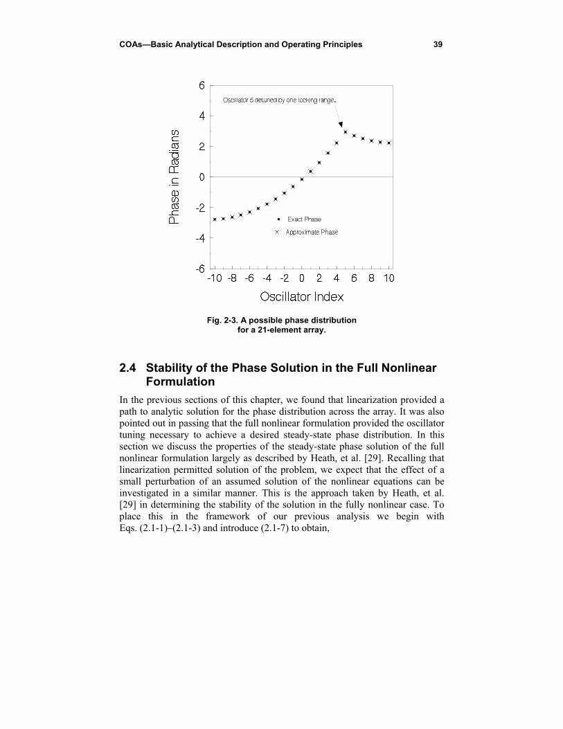
COAs—Basic Analytical Description and Operating Principles 39
Fig. 2-3. A possible phase distribution
for a 21-element array.
2.4 Stability of the Phase Solution in the Full Nonlinear Formulation
In the previous sections of this chapter, we found that linearization provided a path to analytic solution for the phase distribution across the array. It was also pointed out in passing that the full nonlinear formulation provided the oscillator tuning necessary to achieve a desired steady-state phase distribution. In this section we discuss the properties of the steady-state phase solution of the full nonlinear formulation largely as described by Heath, et al. [29]. Recalling that linearization permitted solution of the problem, we expect that the effect of a small perturbation of an assumed solution of the nonlinear equations can be investigated in a similar manner. This is the approach taken by Heath, et al. [29] in determining the stability of the solution in the fully nonlinear case. To place this in the framework of our previous analysis we begin with Eqs. (2.1-1)–(2.1-3) and introduce (2.1-7) to obtain,
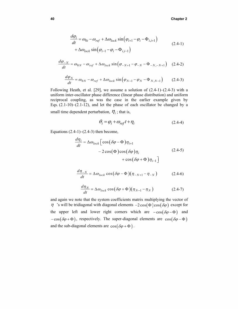
40 Chapter 2
0 1 , 1
1 , 1
sin
sin
ii ref lock i i i i
lock i i i i
d
dt
(2.4-1)
0 1 , 1sinNN ref lock N N N N
d
dt
(2.4-2)
0 1 , 1sinNN ref lock N N N N
d
dt
(2.4-3)
Following Heath, et al. [29], we assume a solution of (2.4-1)–(2.4-3) with a uniform inter-oscillator phase difference (linear phase distribution) and uniform reciprocal coupling, as was the case in the earlier example given by Eqs. (2.1-10)–(2.1-12), and let the phase of each oscillator be changed by a
small time dependent perturbation, i ; that is,
i i ref it (2.4-4)
Equations (2.4-1)–(2.4-3) then become,
1
1
cos
2 cos cos
cos
ilock i
i
i
d
dt
(2.4-5)
1cosNlock N N
d
dt
(2.4-6)
1cosNlock N N
d
dt
(2.4-7)
and again we note that the system coefficients matrix multiplying the vector of ’s will be tridiagonal with diagonal elements 2 cos cos except for
the upper left and lower right corners which are cos
and
cos , respectively. The super-diagonal elements are cos
and the sub-diagonal elements are cos .
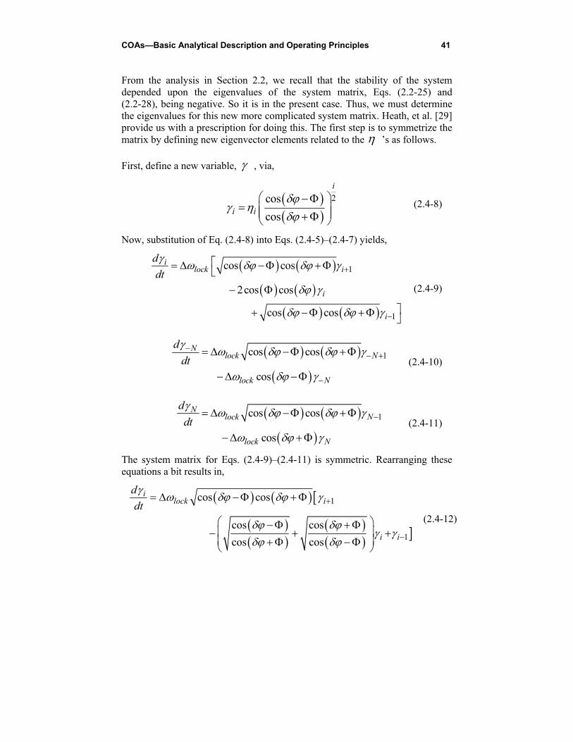
COAs—Basic Analytical Description and Operating Principles 41
From the analysis in Section 2.2, we recall that the stability of the system depended upon the eigenvalues of the system matrix, Eqs. (2.2-25) and (2.2-28), being negative. So it is in the present case. Thus, we must determine the eigenvalues for this new more complicated system matrix. Heath, et al. [29] provide us with a prescription for doing this. The first step is to symmetrize the matrix by defining new eigenvector elements related to the ’s as follows. First, define a new variable, , via,
2cos
cos
i
i i
(2.4-8)
Now, substitution of Eq. (2.4-8) into Eqs. (2.4-5)–(2.4-7) yields,
1
1
cos cos
2cos cos
cos cos
ilock i
i
i
d
dt
(2.4-9)
1cos cos
cos
Nlock N
lock N
d
dt
(2.4-10)
1cos cos
cos
Nlock N
lock N
d
dt
(2.4-11)
The system matrix for Eqs. (2.4-9)–(2.4-11) is symmetric. Rearranging these equations a bit results in,
1
1
cos cos
cos cos
cos cos
ilock i
i i
d
dt
(2.4-12)
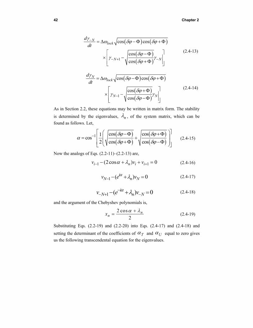
42 Chapter 2
1
cos cos
cos
cos
Nlock
N N
d
dt
(2.4-13)
1
cos cos
cos
cos
Nlock
N N
d
dt
(2.4-14)
As in Section 2.2, these equations may be written in matrix form. The stability
is determined by the eigenvalues, n , of the system matrix, which can be
found as follows. Let,
1 cos cos1cos
2 cos cos
(2.4-15)
Now the analogs of Eqs. (2.2-11)–(2.2-13) are,
1 1(2cos ) 0i n i iv v v (2.4-16)
1 ( ) 0iN n Nv e v (2.4-17)
1 ( ) 0iN n Nv e v
(2.4-18)
and the argument of the Chebyshev polynomials is,
2 cos
2n
nx
(2.4-19)
Substituting Eqs. (2.2-19) and (2.2-20) into Eqs. (2.4-17) and (2.4-18) and
setting the determinant of the coefficients of T and U equal to zero gives
us the following transcendental equation for the eigenvalues.
COAs—Basic Analytical Description and Operating Principles 43
1 1sin 2 1 cos sin 2 1 cos cosn n nx N x N x (2.4-20)
So either,
cosnx (2.4-21)
and, from Eq. (2.4-19) the eigenvalues are zero, or,
1sin 2 1 cos 0nN x
(2.4-22)
and the eigenvalues are,
2 2
2cos 2cos2 1
/ 24sin 4sin
2 1 2
nn
N
n
N
(2.4-23)
The time dependence of the nth perturbation mode will be,
cos cosn lock nt te e
(2.4-24)
and
cos cosn n lock (2.4-25)
Substituting Eq. (2.4-23) into Eq. (2.4-25),
2 2/ 24 sin sin
2 1 2
cos cos
n lockn
N
(2.4-26)
The nth perturbation eigenmode will be stable if n has a non-positive real part.
In general, the phase distribution across the array will be stable if all of the
sn ' have non-positive real parts. Note that in the typical case where is an
44 Chapter 2
integral multiple of , is zero. Then, if is less than 2/ all of the
eigenvalues are real and non-positive so the array phase distribution is stable against small perturbations. In this section we have shown that, by linearizing the equations about an arbitrary solution for the phase distribution in a linear array in which only the end oscillator free running frequencies are controlled, we may study analytically the stability of the solution against small perturbations. Heath, et al. [29] have also shown that exact stable constant phase gradient solutions of the nonlinear equations with arbitrary time dependence can be obtained if one is willing to control the free-running frequencies of all of the oscillators in the array rather than just the end ones.
2.5 External Injection Locking
It was mentioned in passing in Section 2.1 that we chose the number of oscillators in the array to be odd so as to provide a convenient center point at which to inject a stabilizing external signal. In this section we discuss the needed modifications to the mathematical formulation to accommodate an external injection signal and account for its impact on array behavior. Beginning with Eq. (2.1-1) we envision an external signal injected into the pth oscillator and add a term to the equation representing this signal.
0 1 , 1
1 , 1
, , ,
sin
sin
sin
ii lock i i i i
lock i i i i
ip lock p inj inj p p inj
d
dt
(2.5-1)
where ip is the Kronecker delta function and , ,lock p inj is the locking range
between the external oscillator and the injected oscillator in the array. Note that the phase of the injection signal must remain within 2/ radians of that of the injected array oscillator to maintain lock. For simplicity, let all of the coupling phases be zero and assume that the inter-oscillator phase differences are small to permit linearization. Then, introducing Eq. (2.1-7) we have,
0 1 1
, ,
2ii ref lock i i i
ip lock p inj p inj
d
dt
(2.5-2)
COAs—Basic Analytical Description and Operating Principles 45
By replacing Eq. (2.2-4) with Eq. (2.5-2) while Eqs. (2.2-5) and (2.2-6) remain unchanged, Eq. (2.2-9) now becomes,
[ [ ] [ ] [ ]][ ] [ ] [ ]tune injs I M d r (2.5-3)
where [d] is a matrix with one non-zero element, r, at position pp on its
diagonal, [ ]inj is a vector with one non-zero component, the pth one., and
, ,lock p inj
lock
r
(2.5-4)
Here again the tilde denotes Laplace transformation with respect to the scaled time, . Equation (2.2-11) is thus replaced by,
1 1(2 ) 0i ip n i iv r v v (2.5-5)
And Eqs. (2.2-12) and (2.2-13) are unchanged. We now postulate eigenvectors with two sets of elements, those to the left of and including the injection site I = p labeled “L” and those to the right of and including the injection site I = p labeled “R.” That is,
( ) ( ) ( )1( ) ( ) ( );L L L
n i n i ni T UW x T x U x i p (2.5-6)
( ) ( ) ( )1( ) ( ) ( );R R R
n i n i ni T UW x T x U x i p (2.5-7)
and we require that the pth elements match at the injection site; that is,
( ) ( )( ) ( )L Rp n p nW x W x (2.5-8)
Now Eq. (2.5-5) with i=p, Eq. (2.2-12), Eq. (2.2-13), and Eq. (2.5-8) are four
equations in the four unknowns, ( )LT ,
( )LU ,
( )RT , and
( )RU . The equations
are homogeneous, so the determinant of the coefficients must be zero if we are to obtain a nontrivial solution. As usual, this condition yields a transcendental
equation for nx thus giving the eigenvalues, n . The transcendental equation
in this case is,

46 Chapter 2
1 1
1 1
sin cos sin (2 1)cos
1 1cos ( )cos cos ( )cos
2 2
n n
n n
x N x
r N p x N p x
(2.5-9)
Note that if r = 0 we recover the eigenvalues for the uninjected array, Eqs. (2.2-24) and (2.2-27). Proceeding as in the uninjected case, the solution may be expressed in terms of the eigenvectors and eigenvalues in the form,
2
0
[ ] [ ] [ ][ ] [ ]
( )[ ] [ ]
Ntune inj n
nn n nn
vv
s v v
(2.5-10)
and the inverse Laplace transform follows immediately. For practice, you may wish to explicitly compute the eigenvalues and eigenvectors and evaluate the solution from Eq. (2.5-10). The beam-steering scheme proposed by Stephan [1] requires two injection points, i = pL and i = pR, characterized by two locking-range ratios, rL and rR. The solution procedure described above can be generalized to accommodate such a situation as follows. We postulate eigenvectors in three parts, one to the left of both injection points denoted “L”, one between the injection points denoted “B”, and one to the right of both injection points denoted “R.” The elements of these vectors are linear combinations of Chebyshev polynomials as
before. Thus, there will be six unknown coefficients, ( )LT ,
( )LU ,
( )BT ,
( )BU ,
( )RT , and
( )RU . Imposing the end conditions, continuity at each injection
point, and the modified three term recurrence at each injection point,
1 1(2 ) 0L L Lp L n p pv r v v (2.5-11)
1 1(2 ) 0R R Rp R n p pv r v v (2.5-12)
provides a homogeneous system of six equations for these unknown coefficients. Setting the determinant of this system equal to zero yields a transcendental equation for the eigenvalues and the solution proceeds as before. This transcendental equation is,
COAs—Basic Analytical Description and Operating Principles 47
1 1
1 1
1 1
11
1
sin cos sin (2 1)cos
1 1cos ( ) cos cos ( ) cos
2 2
1 1cos ( ) cos cos ( ) cos
2 2
cos (2 1 2 )cossin cos
cos (2 1 2 )cos sin ( ) c
n n
L L n L n
R R n R n
L RL n
n
R n R L
x N x
r N p x N p x
r N p x N p x
r rN p x
x
N p x p p
1os 0nx
(2.5-13)
Note that if either rL or rR is zero, we recover Eq. (2.5-9). Here again you may want to perform the detailed calculations to obtain the explicit solution. Solutions of this type will be discussed in further detail in connection with the continuum model treated in Chapter 3. In the extreme case where all of the oscillators are injection locked to the same external oscillator, the solution simplifies considerably. Returning to Eq. (2.5-3), we find that the elements of [d] are all equal as are the elements of
[ ]inj . So that Eq. (2.5-3) becomes,
[ [ ] [ ][ ] [ ]tunes I M (2.5-14)
where,
[ ] [ ] [ ]M M d (2.5-15)
and
[ ] [ ] [ ]tune tune injr (2.5-16)
Eq. (2.5-14) is now identical in form to Eq. (2.2-9), and the solution in the form of Eq. (2.2-34) follows immediately. However, if the injection signals differ sufficiently in phase, the elements of the right side of Eq. (2.5-16) can exceed unity and the oscillators therefore lose lock. This phenomenon has been exploited in discriminating between signals arriving at disparate angles in illuminating a phased array. For a given illumination angle the signals at each element differ from those of nearest neighboring elements by a constant phase difference and, if used to inject the corresponding oscillators of a coupled oscillator array, represent the second term on the right side of Eq. (2.5-16). Thus, as the incidence angle increases, the phase differences increase and
48 Chapter 2
eventually the array loses lock. This permits identification of signals arriving outside a given range of incidence angles. [18] Before proceeding to planar arrays, we remark at this point that one may also produce beam-steering via a variant of the Stephan approach in which the external injection signals are provided by the end oscillators of the array and their phase is controlled by adjusting the coupling phase between the end and next to end oscillators [30]. Finally, we add that, as shown by Heath, control of the coupling phase also affords the possibility of creating a so-called “difference pattern” in which a null is formed instead of a beam. [31] This is done by switching the phase of one interior coupling by π radians. Of course, such a null can also be steered via either detuning or injection of the end oscillators.
2.6 Generalization to Planar Arrays
Nearly all of the formalism presented in connection with linear arrays of oscillators can be generalized to planar arrays. The simplest of planar arrays consists of a linear array of linear arrays placed side by side as shown in Fig. 2-4. Assuming nearest-neighbor coupling, this implies that each oscillator is coupled to four others and can be described mathematically by analogy with Eq. (2.1-1). That is,
0 1,
1,
, 1
, 1
sin
sin
sin
sin
ijij lock i j ij
lock i j ij
lock i j ij
lock i j ij
d
dt
(2.6-1)
where, for simplicity, we have assumed that all of the coupling phases are equal. The oscillators are indexed separately in the two orthogonal directions x and y in the plane of the array by indices i and j, respectively. The four sine terms correspond to coupling to the four nearest neighboring oscillators implying that for a zero-coupling phase, the center oscillator may be detuned by as much as four locking ranges, and the array will still remain locked. Similarly, the corner oscillators may be detuned by two locking ranges. The largest permitted detuning of the other oscillators will lie between two and four locking ranges. The effects of a uniform coupling phase can be determined in
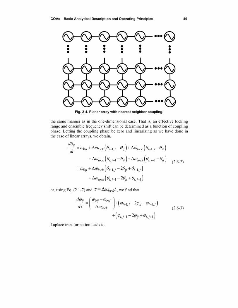
COAs—Basic
the same marange and enphase. Lettinthe case of lin
d
dt
or, using Eq.
Laplace trans
c Analytical De
Fig. 2-4. Plan
anner as in thsemble freque
ng the couplinnear arrays, w
0
0
ijij
ij
t
(2.1-7) and
ijd
d
sformation lea
escription and
nar array with
he one-dimensency shift canng phase be zwe obtain,
1,
, 1
1,
, 1
lock i j
lock i j
lock i j
lock i j
lockt ,
0ij ref
lock
ads to,
d Operating Pr
h nearest neigh
sional case. Tn be determinzero and line
1,
,
2
2
ij lo
ij lo
ij i j
ij i j
, we find that
1,
, 1
2
2
i j
i j ij
rinciples
hbor coupling
That is, an efned as a functiearizing as w
1,
, 1
1
ock i j
ock i j
j
t,
1,
, 1
ij i j
i j
4
g.
ffective lockinion of coupline have done
ij
ij
(2.6-2)
(2.6-3)
49
ng ng in
50 Chapter 2
1, 1,
, 1 , 1
2
2
ij tune i j ij i j
i j ij i j
s
(2.6-4)
where, 0[ ] ij reftune
lock
, elements of a rectangular matrix. This
equation may now be written in matrix form by defining a matrix [ ] with
elements ij . We now define eigenmatrices, [ ]v , with elements, ijv , and
eigenvalues, mn , satisfying,
1, 1, , 1 , 12 2i j ij i j i j ij i j mn ijv v v v v v v (2.6-5)
The key concept enabling analytical treatment of planar arrays is separability of the behavior in the two orthogonal directions. That is, if we define the two dimensional phase distribution to be the product of two one dimensional distributions,
ij i jv v v (2.6-6)
Then Eq. (2.6-5) becomes,
1 1 1 12 2j i i i i j i j mn i jv v v v v v v v v v (2.6-7)
Dividing by the product, jivv , results in,
1 11 1
22 j j ji i imn
i j
v v vv v v
v v
(2.6-8)
The first term on the left is dependent only on i and is independent of j. Similarly the second term on the left is dependent only on j and is independent of i. The right side of the equation is independent of both i and j. Thus, we have a sum of a function of i and a function of j equal to a constant which implies that each of these functions must itself be a constant. That is,
1 12i i i
mi
v v v
v
(2.6-9)
COAs—Basic Analytical Description and Operating Principles 51
1 12j j j
nj
v v v
v
(2.6-10)
and
m n mn (2.6-11)
Using the definition of [M] from Eq. (2.2-7), we may write Eqs. (2.6-9) and (2.6-10) in the forms,
[ ]][ ] [ ]m m mM v v (2.6-12)
and
[ ]][ ] [ ]n n nM v v (2.6-13)
which are identical to Eq. (2.2-10). Thus, the eigenmatrices have been separated into the outer product of eigenvectors, one for the i dependence and one for the j dependence, and each of these eigenvectors is identical with those of the linear array of section 2.2. That is,
[ ] [ ] [ ]mn m nv v v (2.6-14)
The eigenvectors and eigenvalues of Eqs. (2.6-12) and (2.6-13) were found in section 2.2, and we will use them here to express the solution of Eq. (2.6-4) in the form,
[ ] [ ]mn mnm n
C v (2.6-15)
Substitution of this form into Eq. (2.6-4) gives,
[ ] [ ]
[ ]
mn mn tune m mn mnm n m n
n mn mnm n
s C v C v
C v
(2.6-16)
We now make use of the orthogonality of the eigenvectors. Premultiplying by
[ ]pv and post multiplying by [ ]qv , we have,
52 Chapter 2
[ ] [ ] [ ] [ ] [ ] [ ]
[ ] [ ] [ ] [ ]
pq p p q q p tune q
p q p p q q
sC v v v v v v
v v v v
(2.6-17)
so that,
[ ] [ ]
[ ] [ ] [ ] [ ]
p tune qpq
p q p p q q
v vC
s v v v v
(2.6-18)
And Eq. (2.6-15) becomes,
[ ] [ ]
[ ] [ ][ ] [ ] [ ] [ ]
m tune nmn
m n m m n nm n
v vv
s v v v v
(2.6-19)
the planar analog of Eq. (2.2-33). The stability analysis of Section 2.4 also carries over to the planar case as discussed by Heath, et al. [29]. One may similarly derive a planar analog of (2.5-10) should there be external injection [2]. The dynamic behavior of the phase distribution for these cases will be discussed in greater detail in connection with the continuum model presented in Chapter 3. However, we remark here that Karl Stephan and his student, William Morgan, reported application of his external injection beam-steering technique to a four-by-four planar array of mutually injection-locked oscillators [2]. They also developed a theory for such arrays in which the coupling is accomplished via a general multiport coupling network described by an admittance matrix as will be further described in Section 2.7 [2] [3]. They considered theoretically the use of such an oscillator array to excite an array of tapered slot radiators reasoning that the higher gain of these elements would mitigate grating lobes if the array size were increased by using element spacing greater than a half wavelength.
2.7 Coupling Networks
So far we have focused primarily on the behavior of the oscillators in the array but very little on the manner in which they are coupled. We merely asserted that the coupling was present with a certain assumed strength and coupling phase. In addition, two other parameters are important in the design of coupled-oscillator arrays, the network quality factor or Q, which is related to the bandwidth, and the load presented to the oscillators by the network. Although not essential, two simplifying assumptions are quite commonly made. The coupling strength is assumed to be weak in a sense to be detailed shortly, and
COAs—Basic Analytical Description and Operating Principles 53
the coupling network Q is assumed to be small relative to the oscillator Q so that the network can be assumed to be frequency independent over the operating bandwidth of the oscillators. Finally, it is essential that the load resistance presented to the oscillators be smaller than the maximum negative resistance the oscillator can produce so that oscillation can be sustained. In order to systematically design appropriate coupling networks, it is necessary to derive relationships between these three parameters and the values of the components used in constructing the network. In this section, such relationships will be derived. Before proceeding, we remark that the consequences of violation of the above simplifying assumptions have in fact been studied. The case of strong coupling was treated in this context by Nogi, et al. [17]. They showed that strongly coupled arrays exhibit many modes in which the oscillator amplitudes as well as the phases vary across the array and that only one mode has constant amplitude. They further suggested that all other modes can be suppressed by placing a series resistor at the center point of each coupling line. The principle underlying this approach was pointed out very early by Stephan and Young. [3] The implications of narrow-band coupling networks were studied by Lynch and York [32]. The analysis becomes more complicated than in the broadband case [33], but useful results can still be obtained. Very recently these issues were re-examined by Seetharam and Pearson [19]. They showed that strongly coupled oscillator arrays exhibit wider locking ranges and lower phase noise levels but that the broadband assumption concerning the coupling network is violated, necessitating the use of the more complicated theoretical formalism. Generally, the oscillators may be viewed as being coupled by a multiport passive network to which an oscillator is to be connected at each port. This situation was analyzed by Pogorzelski [34]. The network is characterized by its complex admittance matrix; and for a linear array, if the desired coupling is to nearest neighbors, then the admittance matrix will be tridiagonal. For analytical simplicity, we assume an infinitely long array. We want the oscillators to operate in identical environments, so we design the network to be periodic with period unity in the oscillator index. Its admittance matrix will therefore have equal diagonal elements, Y11, and equal off-diagonal elements, Y12. Focusing now on the network alone, in terms of the complex impedance matrix we may write the network equations in the form,
port portZ I V (2.7-1)
54 Chapter 2
where the vector components are the port currents and port voltages. Because
the network is periodic, the elements of the impedance matrix, mnZ will have
the form,
mn n mZ Z Z (2.7-2)
where the port indices, m and n, extend from minus infinity to plus infinity for this infinite network. In this sense, denotes the “distance of the element from the main diagonal of the matrix.” Furthermore, the network periodicity implies
that the components of the eigenvectors, w , of the impedance matrix will
have uniform phase progression and uniform amplitude across the network ports. That is, the elements of the eigenvector with inter-port phase difference are,
jmmw e (2.7-3)
Defining,
portI I w (2.7-4)
and
portV V w (2.7-5)
every equation in the system given by Eq. (2.7-1) becomes,
j
n
Z e I V
(2.7-6)
Now, the tridiagonal admittance matrix gives us,
11 12 12j jI V Y Y e Y e
(2.7-7)
Combining Eqs. (2.7-6) and (2.7-7), we have,
11 12
1
2 cosj
n
Z eY Y
(2.7-8)
COAs—Basic Analytical Description and Operating Principles 55
a Fourier series for which the coefficients, Z , can be found by means of the
usual integration. That is,
11 12
1
2 2 cos
je dZ
Y Y
(2.7-9)
The integration can be carried out analytically to yield,
2 2
11 12 11
2 2 1211 12
41
24
Y Y YZ
YY Y
(2.7-10)
This approach is quite similar to that used in the analysis of phased-array antennas to obtain the well-known relationship between the mutual coupling coefficients among the elements and the active reflection coefficients of the array [35]. The result is that we have expressed the elements of the impedance matrix and admittance matrix of the coupling network in terms of the two parameters, Y11 and Y12. We now define the complex coupling coefficient of the coupling network in the following way. Let the voltage at the nth port be Vn and the current into the nth port be In. We can establish a Norton equivalent circuit at the (n+1)st port as follows. The open circuit voltage is,
1oc nV I Z (2.7-11)
and the short circuit current is,
12sc nI VY (2.7-12)
Thus, the Norton admittance is,
2 2 2 2
11 12 11 11 1212 12
1 11 1 11
4 4
2n
Nn
Y Y Y Y YV Y YY
I Z Y Z Y
(2.7-13)
Now, using the Norton equivalent circuit and connecting load admittance GL to the port, the voltage at port n+1 is,
12
11
n sc nL N L N
YV I V
G Y G Y
(2.7-14)
56 Chapter 2
The complex coupling coefficient, , is defined to be the ratio of the voltage at port n+1 to the voltage at port n. That is,
12
L N
Y
G Y
(2.7-15)
In the weak coupling approximation, Y12 is small and to first order in Y12, we have,
12
L
Y
G (2.7-16)
This coupling factor determines the locking range because the injection signal arriving at an oscillator, i, from a neighboring one, j, is the amplitude of the
oscillator signal, Aj, multiplied by so the locking range is given by,
0 12 0
2 2ji i
locki L
A Y
Q A QG
(2.7-17)
For comparison, see Eq. (1.3-16). Before proceeding, we wish to highlight an interesting point regarding the nature of the coupling. If a current is injected into the nth port of the network with all other ports open circuited, the voltage appearing at port n+m is, from the impedance matrix, just Zm/Z0 times the voltage at the injected port. (See Eq. (2.7-10).) That is, open-circuit voltages appear at all ports throughout the network, not just at the adjacent ports. In this sense, each oscillator really influences all the others, and the coupling is “all to all” rather than “nearest neighbor” in nature. The fact that the admittance matrix is banded might seem to imply nearest-neighbor coupling, but the banded nature of the matrix merely implies that, when a voltage is applied to the nth port with all the other ports shorted, short-circuit current flows only in the adjacent ports. The limited influence results from shorting the ports not from limited coupling. That said, we proceed to define the coupling factor of the network, as the ratio of the open-circuit voltages at adjacent ports when a current is injected into the nth port of the network with all other ports open circuited. From Eq. (2.7-10), that ratio is,
2 2
11 12 11
12
4
2
Y Y Y
Y
(2.7-18)
For weak coupling, this becomes,
COAs—Basic Analytical Description and Operating Principles 57
12
11
Y
Y (2.7-19)
where we have effectively neglected the coupling to the non-nearest neighbor ports by working only to first order in this ratio. This same result is obtained if we define the coupling factor by applying a voltage to the nth port, shorting all the others and taking the ratio of the (n+1)st port current to the nth port current. This obtains because if GL is large compared to Y12, the coupling is weak and the ports are all nearly shorted. The coupling factor appearing in the expression for the locking range given by Eq. (2.7-17) depends on both the oscillator load and the coupling network. Based on the discussion above, we can separate these by writing Eq. (2.7-16) in the form,
12 11
11 L
Y Y
Y G
(2.7-20)
so that the first factor, , characterizes the network coupling and the second factor, , characterizes the coupling of the oscillators to the network. The second important parameter in network design is the network quality factor or Q. Fundamentally, Q is defined in terms of energy stored and energy lost per unit time, but equivalently, Q can also be defined in terms of the frequency dependence of the port admittance near resonance; that is,
2
res
Y
QY
(2.7-21)
a unitless quantity. For our coupling network we thus have the formula,
11 12
11 12
2 cos
2 2 cos
res
net
Y YQ
Y Y
(2.7-22)
And, for our formulation to apply, this must be much smaller than the Q of the oscillators.
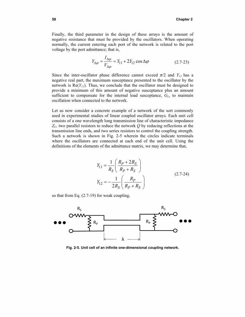
58 Chapter 2
Finally, the third parameter in the design of these arrays is the amount of negative resistance that must be provided by the oscillators. When operating normally, the current entering each port of the network is related to the port voltage by the port admittance; that is,
11 122 cosI
Y Y YV
(2.7-23)
Since the inter-oscillator phase difference cannot exceed π/2 and Y12 has a negative real part, the maximum susceptance presented to the oscillator by the network is Re(Y11). Thus, we conclude that the oscillator must be designed to provide a minimum of this amount of negative susceptance plus an amount sufficient to compensate for the internal load susceptance, GL, to maintain oscillation when connected to the network. Let us now consider a concrete example of a network of the sort commonly used in experimental studies of linear coupled oscillator arrays. Each unit cell consists of a one wavelength long transmission line of characteristic impedance ZC, two parallel resistors to reduce the network Q by reducing reflections at the transmission line ends, and two series resistors to control the coupling strength. Such a network is shown in Fig. 2-5 wherein the circles indicate terminals where the oscillators are connected at each end of the unit cell. Using the definitions of the elements of the admittance matrix, we may determine that,
11
12
21
1
2
P S
S P S
P
S P S
R RY
R R R
RY
R R R
(2.7-24)
so that from Eq. (2.7-19) for weak coupling,
Fig. 2-5. Unit cell of an infinite one-dimensional coupling network.
RP
RSRS
RP
λ
COAs—Basic Analytical Description and Operating Principles 59
12
11
1
2 2P
P S
Y R
Y R R
(2.7-25)
and the oscillators must provide negative susceptance, -Gosc, where,
1121
Re P Sosc
S P S
R RG Y
R R R
(2.7-26)
In order to determine the network Q using Eq. (2.7-22), it is necessary to explicitly display the frequency dependence of the admittance parameters induced by the transmission lines. That is, from transmission line theory, we have,
11
1 1cosh sinh sinh cosh
2cosh sinh sinh cosh
R C R Cp C
s sR C R C
R C
Z Z Z ZR Z
YR R
Z Z Z ZZ Z
(2.7-27)
12cosh sinh sinh cosh
R
s
s sR C R C
R C
Z
RY
R RZ Z Z Z
Z Z
(2.7-28)
where ZR is the impedance of the parallel combination of Rp and Rs, and γ is the propagation constant of the transmission line. The frequency dependence arises because is linear in . Using these expressions in Eq. (2.7-22), we find that,
1cos
2
2cos
C CR R
C R C Rnet
s s
R p
Z ZZ Z
Z Z Z ZQ
R R
Z R
(2.7-29)
(Note that this does not agree with equation (18) of [34] due to an algebraic error in the derivation of that equation.) Typical oscillators used with this network have Q’s on the order of 100. To minimize the Q of the network, we chose parameter values to minimize reflections at the ends of the transmission
60 Chapter 2
lines. That is we chose R CZ Z so that for small inter-oscillator phase
differences we have,
4
pnet
s
RQ
R
(2.7-30)
and for resistors of comparable value, the network Q is of order unity, clearly much smaller than the oscillator Q as assumed in the mathematical model. Another particularly simple coupling network was proposed by Humphrey and Fusco; that of a single capacitor between adjacent ports of the network. [36] The corresponding parameters can be derived from the previous example by setting Rp to infinity and replacing Rs by 1/(2jωC). Thus,
11
12
2Y j C
Y j C
(2.7-31)
Note that the approximation of Eq. (2.7-19) is not valid for this network so Eq. (2.7-18) must be used and we obtain,
2 211 12 11
12
41
2
1
20
net
osc
Y Y Y
Y
Q
G
(2.7-32)
Note further that the coupling phase is zero. The approach outlined above for coupling networks designed for linear arrays of oscillators can be generalized to the case of planar arrays in which, for example, each oscillator is coupled to its four nearest neighbors via the network unit cell shown in Fig. 2-5. The admittance matrix is then block tridiagonal, and each diagonal block is tridiagonal while the off-diagonal blocks are diagonal. The matrix is symmetric, and the elements along any diagonal are equal. Thus, the admittance matrix has only three independent elements. The diagonal elements are denoted by Yd, the off diagonal elements of the diagonal blocks by Yx, and the diagonal elements of the off-diagonal blocks by Yy.. As shown in [34], the integral in Eq. (2.7-9) then becomes the two dimensional integral,
COAs—Basic Analytical Description and Operating Principles 61
2
1
2 cos 2 cos4
jmu jnv
mnd x y
e e dudvZ
Y Y u Y v
(2.7-33)
The impedance matrix, though full, also has a block structure. The elements along any diagonal within a block are equal. Similarly, the blocks along any block diagonal are equal. Using a generalization of the notation used previously for the linear case, the first subscript indicates the “distance” from the diagonal within each block and the second subscript indicates the “distance” of the block from the block diagonal. The integrals given by Eq. (2.7-33) for nearest neighbors, Z01 and Z10, as well as the integral for the diagonal elements Z00, can be expressed in terms of elliptic integrals. That is,
00 22 22
162
44
x y
d x yd x y
Y YZ K
Y Y YY Y Y
(2.7-34)
01 22 22
22
1622
2 44
2 2 4 16, ,
2 2 2 2 4
x yd x
y d x yd x y
d x y y x y
y d x y d x y
Y YY YZ K
Y Y Y YY Y Y
Y Y Y Y Y Y
Y Y Y Y Y Y Y
(2.7-35)
10 22 22
22
2 162
2 44
2 2 164, ,
2 2 2 2 4
d y x y
x d x yd x y
d x y x yx
x d x y d x y
Y Y Y YZ K
Y Y Y YY Y Y
Y Y Y Y YY
Y Y Y Y Y Y Y
(2.7-36)
where K is the complete elliptic integral of the first kind and is the elliptic integral of the third kind. [37] The analogs of the voltage ratio of Eq. (2.7-18) are,

62 Chapter 2
10
00x
Z
Z (2.7-37)
and
01
00y
Z
Z (2.7-38)
These expressions are quite cumbersome. However, as shown in Ref. [34], one may obtain more manageable expressions by evaluating the integrals asymptotically for large subscript via the method of stationary phase when the other subscript is zero. While technically only valid for large index, the form of these expressions exhibits a common ratio between the ports which may be taken to be a measure of the coupling. That is, one obtains,
2
2 21
2 2d y d y
xx x
Y Y Y Y
Y Y
(2.7-39)
and
22 2
12 2
d x d xy
y y
Y Y Y Y
Y Y
(2.7-40)
as the analogs of Eq. (2.7-18). For weak coupling, Yx and Yy are small compared with Yd and we obtain,
2x
xd y
Y
Y Y
(2.7-41)
and
2
yy
d x
Y
Y Y
(2.7-42)
Similarly, the analogs of Eq. (2.7-20) are,
2
2d yx
xd y L
Y YY
Y Y G
(2.7-43)
COAs—Basic Analytical Description and Operating Principles 63
2
2y d x
yd x L
Y Y Y
Y Y G
(2.7-44)
The network Q can again be expressed as the logarithmic derivative of the port admittance with respect to frequency. That is,
2 cos 2 cos
2 2 cos 2 cos
res
d x x y y
netd x y y
Y Y YQ
Y Yx Y
(2.7-45)
Finally, the oscillators must provide negative resistance such that,
Reosc dG Y (2.7-46)
For a network using the coupling configuration shown in Fig. 2-5,
22
1
2
P Sd
S P S
Px y
S P S
R RY
R R R
RY Y
R R R
(2.7-47)
so that,
1
2 4p
x yp s
R
R R
(2.7-48)
22 P S
oscS P S
R RG
R R R
(2.7-49)
and,
cos cos12 2
2 cos cos
2
x yC CR R
C R C Rnet
x ys s
R p
Z ZZ Z
Z Z Z ZQ
R R
Z R
(2.7-50)
For R CZ Z and small inter-oscillator phase differences we again have,
64 Chapter 2
4
pnet
s
RQ
R
(2.7-51)
which is typically much smaller than the oscillator Q. In this section we have discussed the analysis of coupling networks for infinite arrays both linear and planar. Although, in practice the arrays are of course finite, the analysis of infinite arrays is more tractable and provides insight into how the circuit parameters affect the array behavior. Thus, relatively simple approximate formulas obtain for the coupling strength, network Q, and needed oscillator negative resistance in terms of circuit element values facilitating the design of such networks.
2.8 Conclusion
In this chapter, the oscillators of the arrays were treated as individual circuits capable of oscillation in themselves. These were coupled to form a mutually injection-locked system of oscillators. In that sense, the modelling was discrete, and the phase distributions studied were distributions of the phases of the individual oscillator outputs, which (of course) have meaning only in terms of the individual oscillator output signals. In the next chapter, however, we will introduce the concept of the continuum model in which the phase distributions are continuous functions. It is emphasized that the values of these continuous functions still only have physical meaning when the functions are evaluated for arguments corresponding to individual oscillators. Arguments between these are for mathematical convenience and the corresponding function values have no physical significance.
65
Chapter 3 The Continuum Model for Linear Arrays
All of the analysis presented so far has treated each oscillator as a discrete device with an injection port and an output port from which a signal emanates having a discrete phase value relative to a phase reference. For this reason, the mathematical model represented has been termed the discrete model. We emphasize that the discrete model encompasses the dynamic behavior of the oscillator array both nonlinear and, if desired, linearized. No new phenomena are added to this range of capability by means of the formulation to be discussed in the present chapter. However, it will be shown that, provided one is willing to linearize, the so called “continuum model” offers considerable advantage in terms of insight and applicability of familiar mathematical techniques. Although the continuum model is fundamentally approximate primarily because of the linearization, it nevertheless provides intuitive understanding of the behavior of coupled oscillator arrays with small inter-oscillator phase differences, an important special case in terms of practical application. Moreover, it provides a basis for understanding the impact of nonlinearity when the inter-oscillator phase differences increase beyond the limits of accurate linear approximation. The continuum model in this context was suggested by Pogorzelski, et al. [38]. In essence we replace the index identifying the oscillators with a continuous variable such that, when the continuous variable takes on the value of the index for a given oscillator, a continuous function of that variable takes on the value of the phase of that oscillator. Thus, only the values of the function at integer values of its argument have physical meaning. The values between integer
66 Chapter 3
values of the argument serve only to facilitate the formulation in terms of a differential equation.
3.1 The Linear Array without External Injection
To derive the continuum model of a simple linear array of oscillators coupled to nearest neighbors, we begin with Eq. (2.2-4) for the linearized discrete model with zero coupling phase and replace the discrete index i with a continuous variable, x.
0
( , )( , )
( , ) 2 ( , ) ( , )
ref
lock
d x tx t
dtx x t x t x x t
(3.1-1)
where 1x . Now treating ( , )x t as a continuous function of x, expanding each term in a Taylor series about x, and retaining terms up to second order in
x , we obtain,
2
0 2
( , ) ( , )( , ) ref lock
x t x tx t
t x
(3.1-2)
Finally, dividing by the locking range and using the normalized time variable,
lockt , we have,
2
2
( , ) ( , )( , )tune
x xx
x
(3.1-3)
This is the fundamental equation for the continuum model of a simple linear array of oscillators with nearest neighbor coupling and no external injection. It is the well-known diffusion equation. Laplace transformation with respect to time results in,
2
2
( , )( , ) ( , )tune
d x ss x s x s
dx
(3.1-4)
a simple second-order linear differential equation for the transform of the phase distribution. Suppose that the array is infinitely long and that one oscillator is step detuned at time zero by C locking ranges where C is less than two. Without loss of
The Continuum Model for Planar Arrays 67
generality, we may select the detuned oscillator to be the one at x=0. For this situation, Eq. (3.1-4) becomes,
2
2
( , )( , ) ( )
d x s Cs x s x
sdx
(3.1-5)
As discussed in Ref. [38], it might be considered more correct to use, in place of the delta function, a square pulse one unit wide to represent the detuning. However, it is shown in Ref. [38] that the difference in the results is very small, and (in the spirit of the continuum model) the use of the delta function affords considerable convenience with minor impact on the results. The differential equation given by Eq. (3.1-5) has an exact solution in closed form. It is,
( , )2
x sCx s e
s s (3.1-6)
and the inverse Laplace transform is,
2 /(4 )( , ) ( ) ( )
2 2x xC
x C e u x erfc u
(3.1-7)
Figure 3-1 shows a plot of this function over the range 10 10x from time zero to time equal to 250 inverse locking ranges for C = 1. Note that as time goes to infinity, the phase diverges as the square root of the time, never reaching a steady state. This may be viewed as a manifestation of the branch cut of Eq. (3.1-6) in the complex s plane. However, differentiating the phase with respect to time gives the simple expression for the frequency,
2 /(4 )( , ) 1
( )2
ref x
lock
x Ce u
(3.1-8)
and thus the frequency converges to the reference frequency at infinite time as one over the square root of the time. This function is plotted in Fig. 3-2 for C equal to unity. Next, let us consider a finite length array over the range
1 1
2 2a x a . For example, if a = 10 there will be 21 oscillators in the
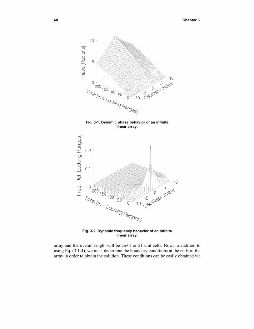
68 Chapter 3
Fig. 3-1. Dynamic phase behavior of an infinite
linear array.
Fig. 3-2. Dynamic frequency behavior of an infinite
linear array. array and the overall length will be 2a+1 or 21 unit cells. Now, in addition to using Eq. (3.1-4), we must determine the boundary conditions at the ends of the array in order to obtain the solution. These conditions can be easily obtained via
The Continuum Model for Planar Arrays 69
an artifice outlined in Ref. [38]. That is, we imagine two additional fictitious oscillators added to the array, one at each end and coupled to the corresponding end oscillator. These oscillators are dynamically tuned so that at all times their phase is maintained equal to the phase of the corresponding end oscillator of the true array. Under these conditions, as may be seen from Eqs. (1.4-1) and (1.4-2), there will be no mutual injection between the end oscillators and the fictitious ones. Thus, the fictitious ones may be removed without effect. However, since the phase of the end oscillator and the corresponding fictitious oscillator are always equal so that the phase difference is zero, and since in the continuum model this difference is represented by the derivative with respect to x, one may conclude that the appropriate boundary condition is that the derivative of the phase with respect to x must be zero; that is, a Neumann boundary condition. At this point, having both the differential equation Eq. (3.1-4) and the boundary conditions, we are in a position to treat the case of a finite length linear array via the continuum model. This will be accomplished using two alternative approaches described below both of which, of course, yield the same result. Before proceeding on this course however, we note an interesting result obtainable directly from the differential equation and the boundary conditions. Suppose we integrate Eq. (3.1-3) over the length of the array.
1 1 122 2 2
21 1 1
2 2 2
( , )( , ) ( , )
a a a
tune
a a a
xdx x dx x dx
x
(3.1-9)
The first term is zero by virtue of the Neumann boundary conditions at the array ends. Thus, we may write,
1 12 2
1 1
2 2
1 1( , ) ( , )
2 1 2 1
a a
tune
a a
x dx x dxa a
(3.1-10)
or,
1 12 2
1 1
2 2
1 ( , ) 1( , )
2 1 2 1
a a
tune ref
a a
xdx x dx
a t a
(3.1-11)
70 Chapter 3
Now from Eq. (1.3-6), neglecting amplitude variation, we have that the instantaneous frequencies of the oscillators are given by,
inst ref t
(3.1-12)
Substituting this into (3.1-11),
1 12 2
1 1
2 2
1 1( , )
2 1 2 1
a a
inst tune
a a
dx x dxa a
(3.1-13)
That is, the average over the array of the instantaneous oscillator frequencies is equal to the average over the array of the oscillator tuning (or free running) frequencies. In steady state the instantaneous frequency is equal to the ensemble frequency. So, we can conclude that the steady-state ensemble frequency of the array is the average of the oscillator tuning frequencies. (Recall the assumption of zero coupling phase.) We now set ourselves the problem of determining the phase dynamics of a finite linear array when one oscillator in the array is step detuned at time zero. The solution of this problem will be a Green’s function permitting solution for an arbitrary distribution of detuning including the antisymmetrical detuning of the end oscillators for beam-steering as suggested by Liao and York [28]. The first approach will be to construct a solution as a superposition of a particular integral and two homogeneous solutions of the differential equation. The particular integral is known from the solution of the infinite array problem. It is essentially Eq. (3.1-6) generalized to accommodate detuning an arbitrary oscillator at x = b instead of the one at x = 0. That is,
( , )2
x b sp
Cx s e
s s (3.1-14)
Adding to this two independent homogeneous solutions with unknown coefficients, CR and CL, we postulate the desired solution in the form,
( , )2
x b s x s x sR L
Cx s e C e C e
s s (3.1-15)
The Continuum Model for Planar Arrays 71
The two unknown coefficients are now determined by applying the boundary
conditions at the two ends of the array, 1
2x a and 1
2x a , resulting in
the two simultaneous linear equations,
1
2b s
R LC
C su C s eu su
(3.1-16)
1
2b s
R LC
C s C su eu su
(3.1-17)
where,
1
( )2
a su e
(3.1-18)
Solving Eqs. (3.1-16) and (3.1-17) simultaneously for CR and CL, we obtain,
2
22
1
21
b s b s
R
Ce e
s s uCu
u
(3.1-19)
and,
2
22
1
21
b s b s
L
Ce e
s s uCu
u
(3.1-20)
The solution given by Eq. (3.1-15) is then,
72 Chapter 3
2
22
2
22
( , )2
1
21
1
21
x b s
b s b s
x s
b s b s
x s
Cx s e
s s
Ce e
s s u eu
u
Ce e
s s u eu
u
(3.1-21)
which simplifies to,
cosh 2 1 cosh( , )
sinh 2 1
C a x b s C x b sx s
s s a s
(3.1-22)
Note that, despite the presence of square roots of s, there are no branch cuts in the s plane because this function is even in the square root of s. Thus, the inverse Laplace transform can be computed purely via residue calculus. The poles, sn, are located by,
sinh 2 1 0n n ns s a s (3.1-23)
Thus,
2
2 1n nn
sa
(3.1-24)
Except for the double pole at s = 0, the residues at these poles are,
cosh 2 1 cosh( 1)
(2 1)
n nnn
n
a x b s x b sresidue C
s a
(3.1-25)
and the residue at the double pole is,
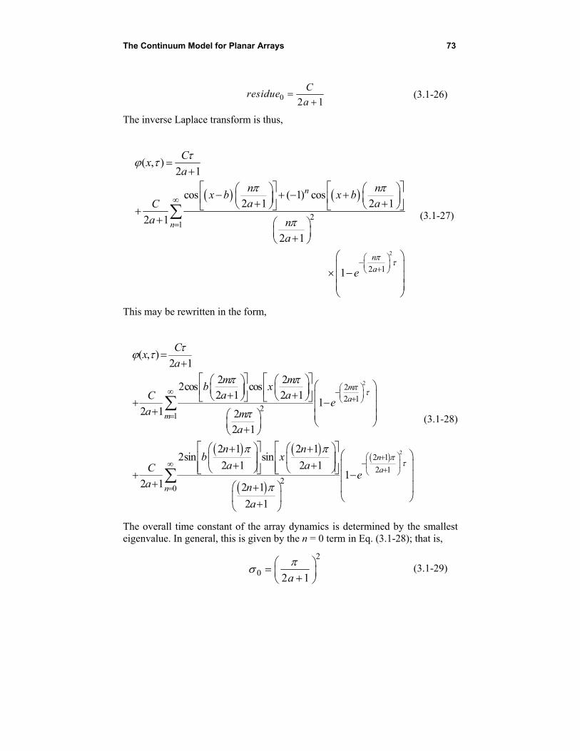
The Continuum Model for Planar Arrays 73
0 2 1
Cresidue
a
(3.1-26)
The inverse Laplace transform is thus,
2
21
2 1
( , )2 1
cos ( 1) cos2 1 2 1
2 1
2 1
1
n
n
n
a
Cx
a
n nx b x b
a aC
a na
e
(3.1-27)
This may be rewritten in the form,
22
2 12
1
20
( , )2 1
2 22cos cos
2 1 2 11
2 1 22 1
2 1 2 12sin sin
2 1 2 11
2 1 2 1
2 1
m
a
m
n
Cx
a
m mb x
a aCe
a ma
n nb x
a aCe
a n
a
22 1
2 1
n
a
(3.1-28)
The overall time constant of the array dynamics is determined by the smallest eigenvalue. In general, this is given by the n = 0 term in Eq. (3.1-28); that is,
2
0 2 1a
(3.1-29)
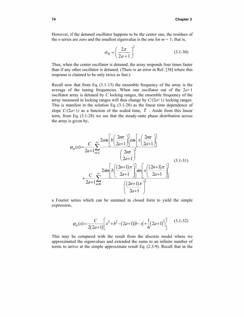
74 Chapter 3
However, if the detuned oscillator happens to be the center one, the residues of the n series are zero and the smallest eigenvalue is the one for m = 1; that is,
2
02
2 1a
(3.1-30)
Thus, when the center oscillator is detuned, the array responds four times faster than if any other oscillator is detuned. (There is an error in Ref. [38] where this response is claimed to be only twice as fast.) Recall now that from Eq. (3.1-13) the ensemble frequency of the array is the average of the tuning frequencies. When one oscillator out of the 2a+1 oscillator array is detuned by C locking ranges, the ensemble frequency of the array measured in locking ranges will thus change by C/(2a+1) locking ranges. This is manifest in the solution Eq. (3.1-28) as the linear time dependence of slope C/(2a+1) as a function of the scaled time, . Aside from this linear term, from Eq. (3.1-28) we see that the steady-state phase distribution across the array is given by,
21
20
2 22cos cos
2 1 2 1( )
2 1 22 1
2 1 2 12sin sin
2 1 2 1
2 1 2 1
2 1
ssn
n
n nb x
a aCx
a na
n nb x
a aC
a n
a
(3.1-31)
a Fourier series which can be summed in closed form to yield the simple expression,
22 2 1( ) 2 1 2 1
2 2 1 6ssC
x x b a b x aa
(3.1-32)
This may be compared with the result from the discrete model where we approximated the eigenvalues and extended the sums to an infinite number of terms to arrive at the simple approximate result Eq. (2.3-9). Recall that in the

The Continuum Model for Planar Arrays 75
linearized discrete model the eigenvalues repeat so, if the sums are continued to an infinite number of terms, a set of delta functions results. Here, in contrast, the sums are in fact infinite and result in a smooth function passing through the correct value of oscillator phase as x passes through the corresponding index of that oscillator. Thus, the two results, discrete and continuum, are only equal at the oscillators and not in between. As indicated in Ref. [38], because the inter-oscillator phase difference cannot exceed 2/ , this steady-state result indicates that the detuning C is limited by,
(2 1)
2
aC
a b
(3.1-33)
However, when operating near the limits of lock, this is not a very good approximation so it is suggested in [38] that the sine terms be approximated by
defining an effective locking range, lock , as follows.
sin( )
sin( )lock lock lock
(3.1-34)
For small phase differences the effective locking range will be nearly equal to the true locking range, but near the limits of lock, it will be /2 times the true locking range. Thus, as pointed out in Ref. [38], though still approximate, the maximum detuning is more accurately given by,
max(2 1)
locka
a b
(3.1-35)
Let us now return to the problem of determining the phase dynamics of a finite linear array when one oscillator in the array is step detuned at time zero and solve it via an alternative approach. We wish to solve Eq. (3.1-5) subject to Neumann boundary conditions at the array ends. Following Pogorzelski, et al. [38] in this alternate approach we first determine the eigenfunctions and eigenvalues defined by,
2
2
d ww
dx (3.1-36)
such that,
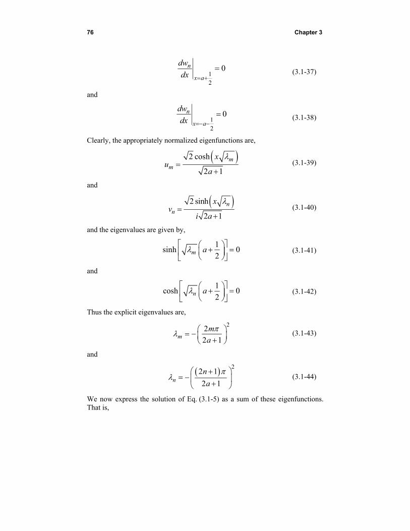
76 Chapter 3
1
2
0n
x a
dw
dx (3.1-37)
and
1
2
0n
x a
dw
dx (3.1-38)
Clearly, the appropriately normalized eigenfunctions are,
2 cosh
2 1
mm
xu
a
(3.1-39)
and
2 sinh
2 1
nn
xv
i a
(3.1-40)
and the eigenvalues are given by,
1
sinh 02m a
(3.1-41)
and
1
cosh 02n a
(3.1-42)
Thus the explicit eigenvalues are,
2
2
2 1mm
a
(3.1-43)
and
22 1
2 1nn
a
(3.1-44)
We now express the solution of Eq. (3.1-5) as a sum of these eigenfunctions. That is,
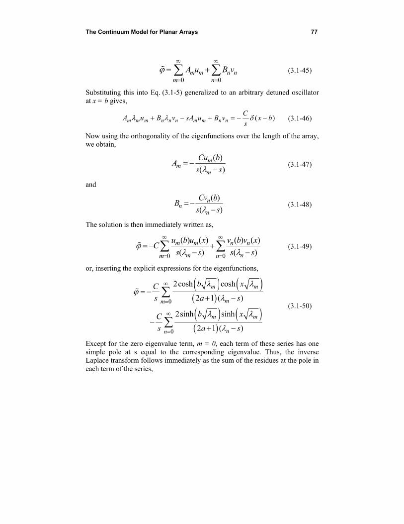
The Continuum Model for Planar Arrays 77
0 0
m m n nm n
A u B v
(3.1-45)
Substituting this into Eq. (3.1-5) generalized to an arbitrary detuned oscillator at x = b gives,
( )m m m n n n m m n nC
A u B v sA u B v x bs
(3.1-46)
Now using the orthogonality of the eigenfunctions over the length of the array, we obtain,
( )
( )m
mm
Cu bA
s s
(3.1-47)
and
( )
( )n
nn
Cv bB
s s
(3.1-48)
The solution is then immediately written as,
0 0
( ) ( ) ( ) ( )
( ) ( )m m n n
m nm n
u b u x v b v xC
s s s s
(3.1-49)
or, inserting the explicit expressions for the eigenfunctions,
0
0
2cosh cosh
2 1 ( )
2sinh sinh
2 1 ( )
m m
mm
m m
nn
b xC
s a s
b xC
s a s
(3.1-50)
Except for the zero eigenvalue term, m = 0, each term of these series has one simple pole at s equal to the corresponding eigenvalue. Thus, the inverse Laplace transform follows immediately as the sum of the residues at the pole in each term of the series,

78 Chapter 3
22
2 12
1
2
20
,2 1
2 22cos cos
2 1 2 11
2 1 22 1
2 1 2 12sin sin
2 1 2 11
2 1 2 1
2 1
m
a
m
n
n
Cx
a
m mb x
a aCe
a ma
n nb x
a aCe
a n
a
2
1
2 1a
(3.1-51)
which is, of course, identical to Eq. (3.1-28). For the case where a = 10 and b = 5, this solution is plotted as a function of time in Fig. 3-3. Note that the shape of the distribution at late times is very much like the corresponding steady-state solution shown in Fig. 2-3. Being the solution for a delta function source on the right side of the differential equation, this is the Green’s function for the problem and as such it can be used to obtain solutions for arbitrary detuning distributions.
Fig. 3-3. Linear array phase distribution under
step detuning of the oscillator at x = 5.
The Continuum Model for Planar Arrays 79
To summarize, we have described two methods of solving the continuum-model partial-differential equation for the dynamic behavior of the phase across a linear array of mutually injection locked oscillators. Both methods entailed Laplace transformation with respect to the scaled time. The first method was a direct solution of the resulting second-order ordinary differential equation by postulating a solution as a superposition of a particular integral and two homogeneous solutions with unknown amplitude coefficients. The coefficients were determined by the Neumann boundary conditions at the array ends. The inverse Laplace transform was obtained as a sum of the residues of at the poles of the transform. In the second method, the Laplace transformed equation was solved by postulating a solution as a sum of eigenfunctions of the second order differential operator each satisfying the Neumann boundary conditions at the array ends. Recognizing this to be a self-adjoint boundary value problem of Sturm-Liouville type, it should not be surprising that the solution for the desired Green’s function can be written as a sum of these eigenfunctions. Conveniently, each term of the sum, except the one corresponding to the zero eigenvalue, has one simple pole so that the inverse Laplace transform is immediately obtainable as a sum of the corresponding residues, one for each term of the eigenfunction series.
3.2 The Linear Array with External Injection
Thus far, the continuum model has been applied to arrays in which the phase control is accomplished by detuning one of the oscillators. The beam-steering method proposed by Stephan [1] requires that two or more array oscillators be injected with an externally derived signal. Thus, to accommodate this, it is necessary to generalize the continuum model along the lines followed in Section 2.5. Following Pogorzelski, et al. [39], we begin with Eq. (2.5-2) rewritten in terms of the continuous variable, x, and the scaled time, , as,
0
, ,
( , )( , ) 2 ( , ) ( , )
( ) ( , ) ( )
i ref
lock
lock p injinj
lock
d xx x x x x
d
x p x
(3.2-1)
Now we define,
, ,( ) ( ) lock p inj
lock
V x x p
(3.2-2)
and expand in a Taylor series about x keeping terms up to second order in xso that Eq. (3.2-1) becomes,
80 Chapter 3
2
2( ) ( ) ( )tune inj
dV x V x
dx
(3.2-3)
Here the spatial distribution of the external injection signals is given by V(x)
while the temporal dependence is given by ( )inj so we have implicitly
assumed that these dependences are separable; that is, all of the injection signal phases have the same time dependence. While this is a convenient simplification, it is not essential in that one could include more than one such injection term in the equation and obtain a solution albeit somewhat more complicated than the one presented here. Equation (3.2-3) is the generalization of Eq. (3.1-3) required to accommodate external injection for our purposes and we will use it to study the phase dynamics of such an externally injected array. Suppose we consider an infinitely long linear array wherein all of the oscillators are tuned to the ensemble or reference frequency and the oscillator at x = b is externally injection locked to an oscillator of strength C with C0 radian step time dependence of its phase. Our generalized differential equation then becomes,
2
02( ) ( ) ( )tune
dC x b CC x b u
dx
(3.2-4)
where,
, ,lock p inj
lockC
(3.2-5)
Laplace transformation with respect to the scaled time results in,
2
02
( ) ( )C
C x b s C x bsx
(3.2-6)
We now define,
01
C
s (3.2-7)
so that Eq. (3.2-6) becomes,
2
11 1 02
( )C x b s Cx
(3.2-8)
The Continuum Model for Planar Arrays 81
The particular integral of this equation is,
01p
C
s (3.2-9)
We postulate a homogeneous solution of the form,
1 1
s x bh C e (3.2-10)
so that our proposed solution is,
01 1
s x bCC e
s (3.2-11)
Now integrating Eq. (3.2-8) across the delta function at x = b, we find that,
11( )
x b
x b
dC b
dx
(3.2-12)
Imposing this condition on the solution given by Eq. (3.2-11), we obtain,
0
12
C CC
s s C
(3.2-13)
Substituting this into the solution given by Eq. (3.2-11) gives,
01 1
2s x bC C
es s C
(3.2-14)
and from Eq. (3.2-7),
0( , )
2
s x bC Cx s e
s s C
(3.2-15)
Finally, the inverse Laplace transform of Eq. (3.2-15) is,
2
0
/2 /4
( , )2
( )2 2
C x b C
x bx C erfc
x be e erfc C u
(3.2-16)
82 Chapter 3
(See Ref. [37] equation 29.3.89.) This is the phase distribution across the infinite array as a function of time. It is zero at time zero and smoothly evolves to a final value of C0 at infinite time as shown in Fig. 3-4 for C0 = 1 radian and C = 1. Note that the injection frequency as well as the initial and final ensemble frequencies are all the same. Because it is the solution for injection at a single point in the array, you might think that it is a Green’s function that can be used to construct solutions for arrays injected at multiple points. However, as we shall see in Section 3.4 when we discuss Stephan’s beam-steering scheme [1] involving two injection points, this is not the case because the form of differential equation itself differs from Eq. (3.2-6) when there are multiple injection points. The corresponding problem where the injected frequency is step shifted by C0 locking ranges at time zero was treated by Pogorzelski, et al. [39]. In that case the array oscillator frequencies evolve from the ensemble frequency at time zero to the injection frequency at infinite time. Next, we consider an array of finite length, 2a + 1, in which all of the oscillators are tuned to the same frequency, taken to be the reference frequency and one of the oscillators, the one at x = b, is injected with an externally generated signal of strength C defined by Eq. (3.2-5) that is step phase shifted at time zero by C0 radians. Equation (3.2-6) applies, but this time we wish to solve it subject to Neumann boundary conditions at the array ends. Here again we have a choice of two methods of solution. Let us begin by postulating the solution in the form of a particular integral plus two complementary functions that are solutions of the homogeneous equation. That is, using Eqs. (3.2-7), (3.2-9), and (3.2-10) we have,
01
s x b x s x sb R L
CC e C e C e
s (3.2-17)
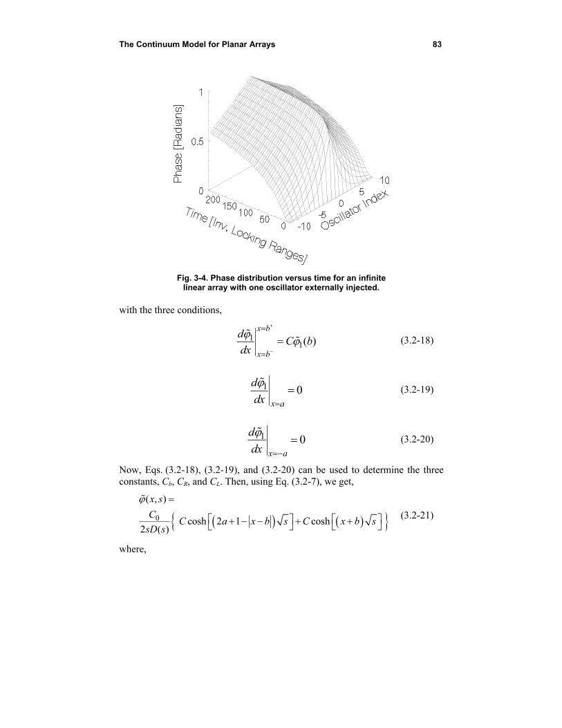
The Continuum Model for Planar Arrays 83
Fig. 3-4. Phase distribution versus time for an infinite
linear array with one oscillator externally injected. with the three conditions,
11( )
x b
x b
dC b
dx
(3.2-18)
1 0x a
d
dx
(3.2-19)
1 0x a
d
dx
(3.2-20)
Now, Eqs. (3.2-18), (3.2-19), and (3.2-20) can be used to determine the three constants, Cb, CR, and CL. Then, using Eq. (3.2-7), we get,
0
( , )
cosh 2 1 cosh2 ( )
x s
CC a x b s C x b s
sD s
(3.2-21)
where,
84 Chapter 3
( ) sinh 2 1
1 1cosh cosh
2 2
D s s a s
C a b s a b s
(3.2-22)
Here again there are no branch cuts, and the inverse Laplace transform is expressible as a sum of residues at the poles; that is, the zeros of D(s), all of which lie on the negative real axis of the s plane. Note that Eq. (3.2-22) is very reminiscent of Eq. (2.5-9) of the discrete model of this array. Comparing these two equations, we may ascertain that the continuum approximation is
particularly accurate for small values of s when sinhs s which, of
course, corresponds to late time. In fact, the pole closest to the origin of the s plane provides us with the time constant of the array which determines the late time behavior. Let us examine Eq. (3.2-22) to see if we can estimate the location of this pole. In anticipation of the fact that the pole lies on the negative real axis, we define so that,
s i i (3.2-23)
Then,
sin 2 1
1 1cos cos
2 2
D a
C a b a b
(3.2-24)
Setting D equal to zero, yields the transcendental equation,
1 12 sin cos
2 2
1 1cos cos
2 2
a a
C a b a b
(3.2-25)
For small , the solution occurs where the cosine functions are near zero and the sine function is near unity. Thus, we define a new variable,
2 1a
(3.2-26)
and write Eq. (3.2-25) in the form,
The Continuum Model for Planar Arrays 85
1 12 sin cos
2 1 2 2 2 2
1cos
2 2 2 1
1cos
2 2 2 1
a aa
bC a b
a
ba b
a
(3.2-27)
or
1 12 cos sin
2 1 2 2
1sin
2 2 1
1sin
2 2 1
a aa
bC a b
a
ba b
a
(3.2-28)
Using the identity for the sine of a sum, we arrive at,
1 12 cos sin
2 1 2 2
1sin cos
2 2 1
1cos sin
2 2 1
1sin cos
2 2 1
1cos
2
a aa
bC a b
a
ba b
a
ba b
a
a b
sin
2 1
b
a
(3.2-29)
Near 0 ,
86 Chapter 3
1cos
2 2 1
sin2 1
1cos
2 2 1
sin2 1
bC a b
a
b
a
ba b
a
b
a
(3.2-30)
which is a quadratic equation for . That is,
22 2
2 2
1
2
sec 2 tan tan 02 1 2 1 2 1
a b
b b bb
C a a a
(3.2-31)
We can now look at two limiting cases. First, if C is small, the solution becomes that of the uninjected array, namely, 0 . If, on the other hand, C is large,
2
2
12
tan2 11
2
b ab
aa b
(3.2-32)
and
2
2
12
tan2 1 2 11
2
b ab
a aa b
(3.2-33)
The Continuum Model for Planar Arrays 87
If b is small; that is, if the injection point is near the center of the array,
2
2
12
2 1 2 112
b ab
a aa b
(3.2-34)
Choosing the sign in the numerator to obtain the solution nearest the origin of the s plane, we have,
2 1 2a b
(3.2-35)
Thus,
2
min 2 1s
a b
(3.2-36)
and that the late time behavior of the array goes as,
2
2 1a be
(3.2-37)
The formula given by Eq. (3.2-33) fails if b is at either end of the array because we have effectively divided by zero in the derivation. We can no longer assume that C is infinite. Retaining a finite value of C and rewriting the transcendental equation results in,
t a n 2 1a C (3.2-38)
If C is small, the solution is approximately,
2 1
C
a
(3.2-39)
but if C is large,
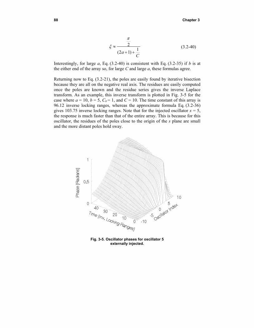
88 Chapter 3
21
(2 1)aC
(3.2-40)
Interestingly, for large a, Eq. (3.2-40) is consistent with Eq. (3.2-35) if b is at the either end of the array so, for large C and large a, these formulas agree. Returning now to Eq. (3.2-21), the poles are easily found by iterative bisection because they are all on the negative real axis. The residues are easily computed once the poles are known and the residue series gives the inverse Laplace transform. As an example, this inverse transform is plotted in Fig. 3-5 for the case where a = 10, b = 5, C0 = 1, and C = 10. The time constant of this array is 96.12 inverse locking ranges, whereas the approximate formula Eq. (3.2-36) gives 103.75 inverse locking ranges. Note that for the injected oscillator x = 5, the response is much faster than that of the entire array. This is because for this oscillator, the residues of the poles close to the origin of the s plane are small and the more distant poles hold sway.
Fig. 3-5. Oscillator phases for oscillator 5
externally injected.
The Continuum Model for Planar Arrays 89
As discussed in connection with the detuned linear array, the above analysis can also be performed by expanding the solution in eigenfunctions of the differential operator. The relevant operator in this case is,
2
2( )C x b
x
(3.2-41)
The presence of the delta function produces a slope discontinuity in the eigenfunctions which must satisfy,
2
2( )n
n n nw
C x b w wx
(3.2-42)
and the boundary conditions,
0n
x a
dw
dx (3.2-43)
0n
x a
dw
dx (3.2-44)
The solution is postulated in the form,
n n nx b x xn b R Lw C e C e C e (3.2-45)
Now we note something interesting about Eq. (3.2-42); that is, it is essentially
Eq. (3.2-6) with C0 set to zero and s set to n . Therefore, we can obtain the
eigenfunctions by means of a limiting process applied to Eq. (3.2-21) instead of solving for the three constants using Eqs. (3.2-42), (3.2-43), and (3.2-44). Suppose we set,
0C (3.2-46)
and,
ns (3.2-47)
in Eq. (3.2-21) and take the limit as approaches zero where n is the nth
value of s for which D(s) equals zero. In this limit both the numerator and
90 Chapter 3
denominator of Eq. (3.2-21) approach zero, but the ratio is finite and
approaches nw . That is,
0
( )
cosh 2 1 cosh
2 ( )
n
n n
n n
w x
C a x b C x b
D
(3.2-48)
But, except for a factor of C0, this is nothing but the residue of Eq. (3.2-21) at the nth pole. Not only have we found the eigenfunctions, but they are already multiplied by the coefficients needed to form the solution by summation except for an overall multiplicative constant of C0. In effect, in Eq. (3.2-48) we are computing,
( )( ) ( )
,n
n nn n n
Cf bw x f x
f f
(3.2-49)
where the bracketed expression in the denominator is the normalizatiintegral; that is, the integral of the square of the arbitrarily normalized eigenfunction, fn, over the array length and,
( ) cosh 2 1 coshn n nf x C a x b C x b (3.2-50)
The desired solution is therefore,
0 0
( ) ( )( , ) ( )
,n n
nn n nn n
f b f xx s C w x C C
f f
(3.2-51)
the well-known form of the solution as a sum of eigenfunctions. Thus, we see that the inverse Laplace transform of the eigenfunction sum representing the solution, ( , )x , is just the sum of the residues of
Eq. (3.2-21) multiplied by the Laplace transform kernel, se . This same property was evident in the treatment of the linear array with one oscillator detuned. It is the reason why Eqs. (3.1-28) and (3.1-51) are identical. Thus, in the present case, we can rest assured that, had we pursued the eigenfunction expansion approach to completion, the result would have been exactly that plotted in Fig. 3–5. The two approaches, the residue series based on the
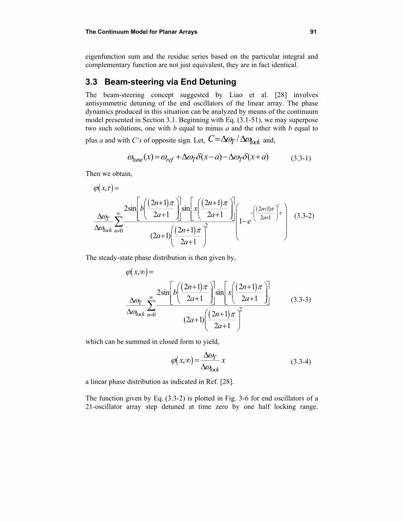
The Continuum Model for Planar Arrays 91
eigenfunction sum and the residue series based on the particular integral and complementary function are not just equivalent, they are in fact identical.
3.3 Beam-steering via End Detuning
The beam-steering concept suggested by Liao et al. [28] involves antisymmetric detuning of the end oscillators of the linear array. The phase dynamics produced in this situation can be analyzed by means of the continuum model presented in Section 3.1. Beginning with Eq. (3.1-51), we may superpose two such solutions, one with b equal to minus a and the other with b equal to
plus a and with C’s of opposite sign. Let, /T lockC and,
( ) ( ) ( )tune ref T Tx x a x a (3.3-1)
Then we obtain,
22 1
2 12
0
,
2 1 2 12sin sin
2 1 2 11
2 1(2 1)
2 1
n
aT
lock n
x
n nb x
a ae
na
a
(3.3-2)
The steady-state phase distribution is then given by,
20
,
2 1 2 12sin sin
2 1 2 1
2 1(2 1)
2 1
T
lock n
x
n nb x
a a
na
a
(3.3-3)
which can be summed in closed form to yield,
, T
lock
x x
(3.3-4)
a linear phase distribution as indicated in Ref. [28]. The function given by Eq. (3.3-2) is plotted in Fig. 3-6 for end oscillators of a 21-oscillator array step detuned at time zero by one half locking range.
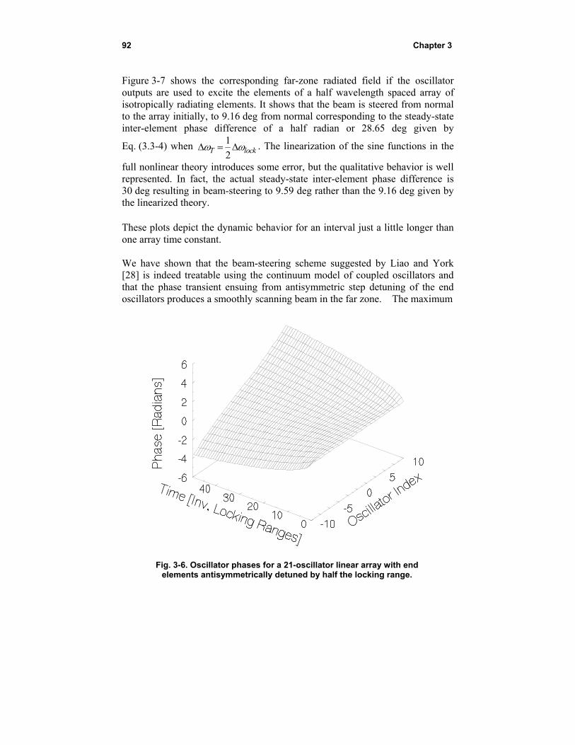
92 Chapter 3
Figure 3-7 shows the corresponding far-zone radiated field if the oscillator outputs are used to excite the elements of a half wavelength spaced array of isotropically radiating elements. It shows that the beam is steered from normal to the array initially, to 9.16 deg from normal corresponding to the steady-state inter-element phase difference of a half radian or 28.65 deg given by
Eq. (3.3-4) when 1
2T lock . The linearization of the sine functions in the
full nonlinear theory introduces some error, but the qualitative behavior is well represented. In fact, the actual steady-state inter-element phase difference is 30 deg resulting in beam-steering to 9.59 deg rather than the 9.16 deg given by the linearized theory. These plots depict the dynamic behavior for an interval just a little longer than one array time constant. We have shown that the beam-steering scheme suggested by Liao and York [28] is indeed treatable using the continuum model of coupled oscillators and that the phase transient ensuing from antisymmetric step detuning of the end oscillators produces a smoothly scanning beam in the far zone. The maximum
Fig. 3-6. Oscillator phases for a 21-oscillator linear array with end elements antisymmetrically detuned by half the locking range.
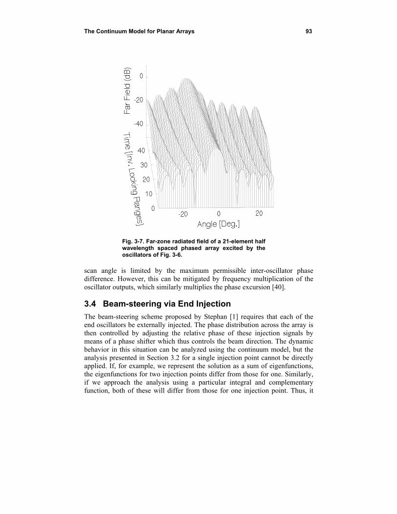
The Continuum Model for Planar Arrays 93
Fig. 3-7. Far-zone radiated field of a 21-element half wavelength spaced phased array excited by the oscillators of Fig. 3-6.
scan angle is limited by the maximum permissible inter-oscillator phase difference. However, this can be mitigated by frequency multiplication of the oscillator outputs, which similarly multiplies the phase excursion [40].
3.4 Beam-steering via End Injection
The beam-steering scheme proposed by Stephan [1] requires that each of the end oscillators be externally injected. The phase distribution across the array is then controlled by adjusting the relative phase of these injection signals by means of a phase shifter which thus controls the beam direction. The dynamic behavior in this situation can be analyzed using the continuum model, but the analysis presented in Section 3.2 for a single injection point cannot be directly applied. If, for example, we represent the solution as a sum of eigenfunctions, the eigenfunctions for two injection points differ from those for one. Similarly, if we approach the analysis using a particular integral and complementary function, both of these will differ from those for one injection point. Thus, it
94 Chapter 3
will be necessary to reformulate the problem for two injection points from the beginning. To be definite, we assume that the oscillators of the array are all initially tuned to the reference frequency and are thus in-phase with each other and that two arbitrary oscillators in the array at x = b1 and x = b2 are injection locked to external signals which are initially in-phase with the oscillators of the array and that at time zero the phase of each of these signals is stepped to a finite constant value. The strengths of the two injection signals are denoted by B1 and B2, and the amplitude of the corresponding temporal step functions are denoted by p1 and p2, respectively. Then, Eq. (3.2-3) becomes,
2
1 1 2 22
1 1 1 2 2 2
( ) ( )
( ) ( ) ( ) ( )
dB x b B x b
dxB x b p u B x b p u
(3.4-1)
Laplace transformation results in,
2
1 1 2 22
1 21 1 2 2
( ) ( )
( ) ( )
B x b B x b sx
p pB x b B x b
s s
(3.4-2)
Now, as shown previously, we may solve this equation either by means of an eigenfunction expansion or by means of superposition of a particular integral and a complementary function. In the former approach, the complexity arises in the normalization of the eigenfunctions, which involves integration of the square of the eigenfunctions of the array. In the latter, this is automatically taken care of by the residues. Thus, we elect to proceed with the latter approach as was done in [39]. The solution of (3.4-2) is postulated in the form,
1 21 2
s x b s x b x s x sR LC e C e C e C e (3.4-3)
The four unknown constants are determined by the boundary conditions at the array ends, Eqs. (3.2-19) and (3.2-20), and the conditions on the derivatives at the injection points, Eq. (3.2-18). These four constraints yield four equations for the four unknowns in Eq. (3.4-3). The solution is,
The Continuum Model for Planar Arrays 95
2
2 2 2 2
2 2
1 1 1 1
1 1
1 2 21
2 1 2 1
1( , )
( )
cosh 2 12
cosh 2 12
cosh 2 12
cosh 2 12
cosh 2 1 22
cosh 2 12
si
x ssD s
sB p a b x b x
sa b x b x
sB p a b x b x
sa b x b x
B B p sa b
s
sa b b b x b x
2 1 2 1
1 2 12
2 1 2 1
2 1 2 1
nh2
cosh 2 1 22
cosh 2 12
sinh2
sb b b x b x
B B p sa b
s
sa b b b x b x
sb b b x b x
(3.4-4)
where,
96 Chapter 3
2
1 1 1
2 2 2
1 22 1
1 2
( ) sinh 2 1
1 1cosh cosh
2 2
1 1cosh cosh
2 2
sinh
1 1cosh cosh
2 2
D s s a s
B s a b s a b
B s a b s a b
B Bs b b
s
s a b s a b
(3.4-5)
Note that, if either of the B’s is zero, we recover Eqs. (3.2-21) and (3.2-22) for a single injection point. The form of the solution presented in Ref. [39] is slightly different but fully equivalent except for a typographical error in
the 1 2sinh 2s b b x term, which should have been
1 2sinh 2s b b x . The pole locations on the negative real axis of the
s plane are easily found by iterative bisection, and the inverse Laplace transform is then obtainable as a residue series. As a first example, we compute the solutions when unit strength injection signals are applied to the end oscillators of a 21-oscillator linear array, and at time zero their phase is step shifted antisymmetrically by one radian producing a phase difference of two radians. The dynamic behavior of the resulting phase distribution is shown in Fig. 3-8. An analytic expression for the steady-state solution for the phase can be obtained by application of the final value theorem to the transform (3.4-4) and (3.4-5). The result is,
1 1 2 2
1 2 1 2 2 1
1 2 2 1 2 1 2 1 2 1
1( , ) 2 2
2 2 2x B p B p
B B B B b b
B B p p b b p p b x b x
(3.4-6)
For the case shown in Fig. 3-8, this expression reduces to,
( , )11
xx (3.4-7)
The Continuum Model for Planar Arrays 97
Fig. 3-8. Phase dynamics for injected end elements.
Notice that the steady-state phases of the injected oscillators at x = 10 and at x = –10 are not equal to the phases of the corresponding injection signals, plus and minus one radian. This is because the end oscillators are also injected by virtue of their coupling to their nearest neighbor in the array, and the phase of that neighbor differs from the phase of the external injection signal. Thus, the total injection of the end oscillator is not in phase with the external injection signal. However, as the strength of the injection signals is increased (large values of the B’s are used), the steady-state phase of the end oscillators will approach the phase of the corresponding injection signals because the signal from the corresponding neighboring oscillators becomes negligible. We again remark, as in Section 2.5, that the injection signals may be derived from the end oscillators of the array and used to inject the next to end oscillators to achieve beam-steering. The continuum model has been used to study this approach also [41]. Recall that the phase of the injection signals can differ from the initial phase of
the injected oscillators by no more than π/2 radians for a maximum total phase
difference of π radians across the array. Thus, for strong injection, the beam-steering angle is limited to a maximum of
98 Chapter 3
1
max sin2 1a S
(3.4-8)
where S is the electrical radiating element spacing in radians. In our present example, if the element spacing is a half wavelength so S = π, then the maximum steering angle is 2.73 deg, a disappointingly small angle. Fortunately, this problem is easily eliminated by gradually increasing the injection phase instead of stepping it. [1] That way, the phase difference between the injected oscillator and the injection signal can be maintained less than π/2 radians while the phase difference between the two injection signals is increased to a large value. The new limit on steering angle is now imposed by the requirement that the inter-oscillator phase difference be less than π/2 radians to maintain overall lock, a limitation also present in the detuning case. In the present example, this limits the steering angle to 30 degrees, a certainly more acceptable limit. As an example of this enhanced beam-steering scheme, we compute the response of the array of the previous example, but this time we gradually increase the injection-signal phase difference by convolving the step function with a temporal Gaussian. By virtue of the linearity of the p dependence of the equation, we may obtain the corresponding phase response by convolving the step response with the same Gaussian. Since the solution is a residue series, each term has simple exponential time dependence so the convolution can be carried out analytically term by term as described in detail in Ref. [39]. Let the Gaussian be,
2( 6) /100( )g e (3.4-9)
Then, setting p2 equal to 2 radians and p1 equal to 2 radians for a total phase difference of 4 radians, the expected steady-state beam-steering angle of a half wavelength spaced array will be 10.48 deg. The steady-state inter-oscillator phase difference is 0.628 radians, for which the sine functions are approximated by their argument with about 7-percent accuracy. However, there are times during the transient at which this difference becomes as large as 0.878 radians near the array ends. At these times, the sine functions are approximated with only 14-percent accuracy. Thus, the actual inter-oscillator phase difference will be somewhat larger. The phase behavior for these parameters and unit amplitude injection as predicted by the continuum model is shown in Fig. 3-9, and the corresponding far zone beam is shown in Fig. 3-10. We have shown the utility of the continuum model in analyzing the transient behavior of linear arrays of mutually injection locked oscillators with external
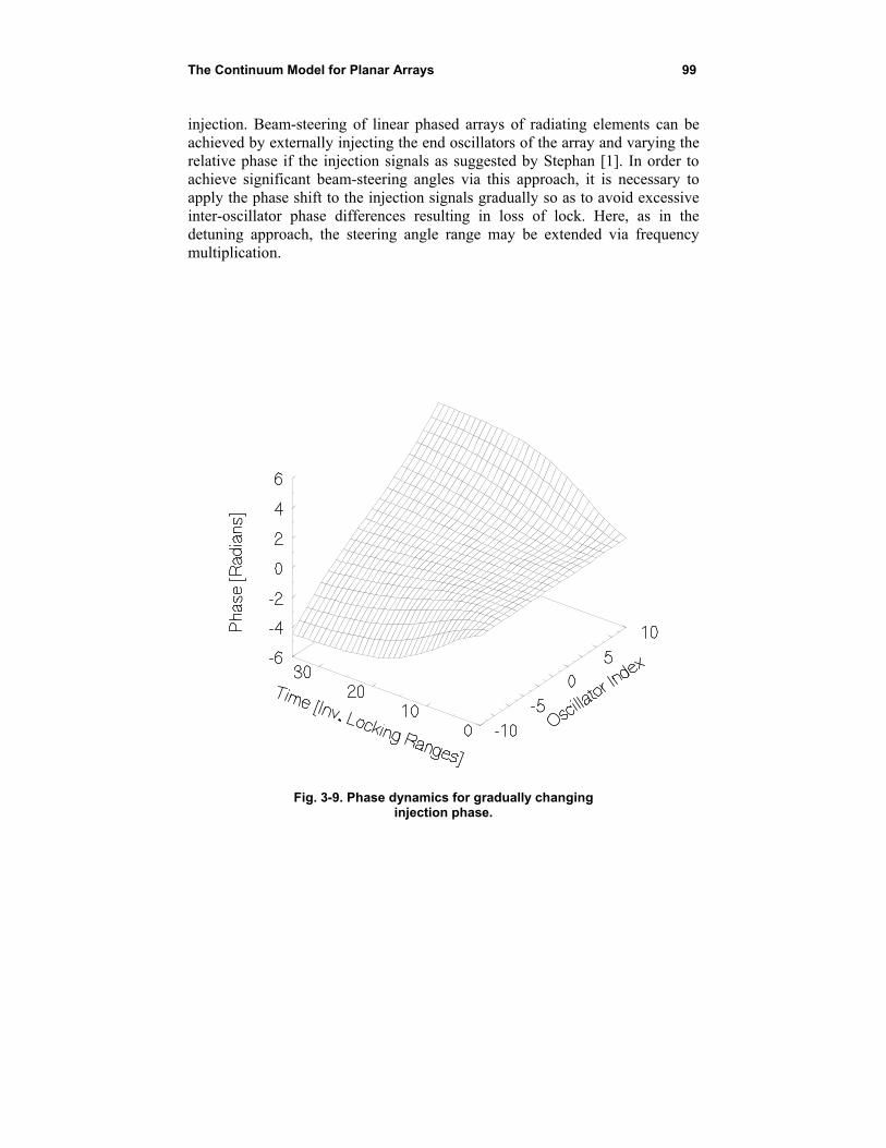
The Continuum Model for Planar Arrays 99
injection. Beam-steering of linear phased arrays of radiating elements can be achieved by externally injecting the end oscillators of the array and varying the relative phase if the injection signals as suggested by Stephan [1]. In order to achieve significant beam-steering angles via this approach, it is necessary to apply the phase shift to the injection signals gradually so as to avoid excessive inter-oscillator phase differences resulting in loss of lock. Here, as in the detuning approach, the steering angle range may be extended via frequency multiplication.
Fig. 3-9. Phase dynamics for gradually changing injection phase.
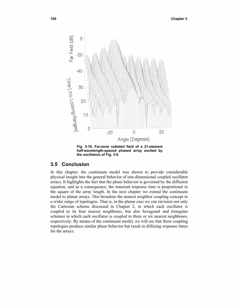
100 Chapter 3
Fig. 3-10. Far-zone radiated field of a 21-element half-wavelength-spaced phased array excited by the oscillators of Fig. 3-9.
3.5 Conclusion
In this chapter, the continuum model was shown to provide considerable physical insight into the general behavior of one-dimensional coupled oscillator arrays. It highlights the fact that the phase behavior is governed by the diffusion equation, and as a consequence, the transient response time is proportional to the square of the array length. In the next chapter we extend the continuum model to planar arrays. This broadens the nearest neighbor coupling concept to a wider range of topologies. That is, in the planar case we can envision not only the Cartesian scheme discussed in Chapter 2, in which each oscillator is coupled to its four nearest neighbours, but also hexagonal and triangular schemes in which each oscillator is coupled to three or six nearest neighbours, respectively. By means of the continuum model, we will see that these coupling topologies produce similar phase behavior but result in differing response times for the arrays.
101
Chapter 4 The Continuum Model for Planar Arrays
As described in Section 2.6, coupled oscillator arrays can be constructed in a planar geometry in which each oscillator is coupled to more than the two nearest neighbors of the linear array case. In that section a Cartesian coupling topology is described in which each oscillator is coupled to four nearest neighbors, and the array boundary is rectangular. In such an arrangement, the phase distributions suitable for beam-steering are obtainable either by detuning the edge oscillators [42] or by injecting them with external signals with adjustable phase [43]. Both of these approaches are treatable via the continuum model. Further generalizing the planar arrangement, one may use alternative coupling topologies such as the triangular lattice in which each oscillator is coupled to six nearest neighbors and the array boundary is triangular or the hexagonal lattice in which each oscillator is coupled to three nearest neighbors and the array boundary is again triangular [44] [45]. As will be shown in this chapter, these coupling topologies are also treatable using the continuum model.
4.1 Cartesian Coupling in the Continuum Model without External Injection
We begin with Eq. (2.6-3) for a 2M + 1 by 2N + 1 rectangular array with zero coupling phase replacing the discrete indices i and j with the continuous variables x and y, respectively; and we expand the phase function in a two-dimensional Taylor series retaining terms to second order. By this process, we obtain the two-dimensional analog of Eq. (3.1-3); that is,
102 Chapter 4
2 2
02 2
( , , ) ref
lock
x yd
d x y
(4.1-1)
or
2 2
2 2 tuned
dx y
(4.1-2)
subject to Neumann boundary conditions at the array edges. (These boundary conditions may be ascertained via the fictitious additional oscillator artifice described in Section 3.1.) Averaging Eq. (4.1-2) over the two dimensional array and using the boundary conditions as in Eqs. (3.1-9) to (3.1-13), it can be shown that the ensemble frequency of the array is the average of the tuning (free running) frequencies of the oscillators. Laplace transformation of Eq. (4.1-2) with respect to the scaled time, , results in,
2 2
2 2 tunesx y
(4.1-3)
where the tilde denotes the transformed function. As in the one-dimensional case, this equation can be solved by postulating a solution as a sum of eigenfunctions of the two-dimensional differential operator, the Laplacian operator, and solving for the coefficients of this expansion. As indicated in [42], the eigenfunctions are,
,,
,,
,,
,,
1cosh cosh
1sinh sinh
1cosh sinh
1sinh cosh
ee mn m nee mn
oo k koo k
eo m mee m
oe kn k noo kn
f s x s yN
f s x s yN
f s x s yN
f s x s yN
(4.1-4)
where the eigenvalues are,
The Continuum Model for Planar Arrays 103
2 2
2 2
2 1 2
2 1 2 1
2 1 2
2 1 2 1
k m
n
k ms s
a a
ns s
b a
(4.1-5)
and the normalization constants are,
,
,
,
,
12 1 2 1
21
2 1 2 121
2 1 2 121
2 1 2 12
ee mn m n
oo k
ee m m
oo kn n
N a b
N a b
N a b
N a b
(4.1-6)
where,
2 ; 0
1; 0mm
m
(4.1-7)
The general solution procedure follows that used in the case of the linear array. That is, we postulate a two dimensional delta function source to obtain the Green’s function as an expansion in the two dimensional eigenfunctions. Then, we integrate the product of this Green’s function and the actual source function over the array to obtain the phase distribution as an expansion in the eigenfunctions. This solution is presented in Ref. [42]. The Green’s function, ( , , , , )g x y x y s , is a solution of,
2 2
2 2( ) ( )
g gs x x y y
x y
(4.1-8)
The solution of this equation expressed as a sum of eigenfunctions is,
104 Chapter 4
, ,
0 0
, ,
0 0
, ,
0 0
, ,
0 0
( , ) ( , )
( , ) ( , )
( , ) ( , )
( , ) ( , )
ee mn ee mn
m nn m
oo k oo k
kk
eo m eo m
mm
oe kn ee mn
k nn k
f x y f x yg
s s s
f x y f x y
s s s
f x y f x y
s s s
f x y f x y
s s s
(4.1-9)
This Green’s function can then be multiplied by the detuning function,
( , , )tune x y s , and integrated over the array. The inverse Laplace transform
is easily obtained as the sum of the residues at the poles as in the one dimensional case. Recall that the detuning of the oscillators required to produce a desired phase distribution across the array can be determined by merely substituting the desired phase distribution into Eq. (4.1-2). From the theory of uniformly spaced phased array antennas, the steady-state phase distribution
necessary to produce a beam steered to spherical coordinate angles, 0 0, ,
with the polar axis normal to the plane of the array, is
( , )2 2
yxss x y x a x a y b y b
(4.1-10)
where,
0 0
0 0
2 sin cos
2 sin sin
x
y
h
h
(4.1-11)
and h is the element spacing while is the wavelength. Substituting into Eq. (4.1-2) with the time derivative set to zero to obtain the steady-state result, we find that,
tune x yx a x a y b y b (4.1-12)
Thus, we discover that beam-steering requires detuning of only the edge oscillators and that the needed detuning is constant along each edge. This leads
The Continuum Model for Planar Arrays 105
us to seek dynamic solutions of Eq. (4.1-2) that result from a temporal step detuning of the edge oscillators that is constant along each edge. That is, we limit ourselves to detuning functions of the general form,
1 2
1 2
( ) ( )
( ) ( )
tune x x
y y
x a u x a u
y b u y b u
(4.1-13)
For step temporal dependence, the Laplace transform of the detuning is,
1 2
1 2
x xtune
y y
x a x as s
y b y bs s
(4.1-14)
The presence of the delta functions facilitates integration of the product of the Green’s function and the tuning function leading to the solution.
2
2
1 21 2
1 22 1
21
1 22 1
21
( , , ) ( )2 1 2 1
( 1) cos1 2 1
1 ( )2 1
2 1
( 1) cos1 2 1
12 1
2 1
y yx x
p px xa
p
p px xa
p
x y ua b
px a
ae u
a pa
px a
ae
a pa
2
2
1 22 1
21
1 22 1
21
( )
( 1) cos1 2 1
1 ( )2 1
2 1
( 1) cos1 2 1
1 ( )2 1
2 1
p py yb
p
p py yb
p
u
px b
be u
b pb
px b
be u
b pb
(4.1-15)
106 Chapter 4
which is the solution for the special case of constant detuning along each edge of the array. In steady state, this reduces to Fourier series that can be summed in closed form resulting in,
1 21 2
2 21 2
1 2
2 21 2
1 2
( , , )2 1 2 1
2 1
2 6 2 1
2
2 1
2 6 2 1
2
y yx x
x x
x x
y y
y y
x ya b
a a xx a x a
a
x a x a
b b yy b y b
b
y b y b
(4.1-16)
which clearly shows that symmetric detuning gives rise to parabolic steady-state phase distributions whereas antisymmetric detuning results in linear steady-state phase distributions. In the antisymmetric case where
1 2x x x and 1 2y y y , Eq. (4.1-16) reduces to
Eq. (4.1-10). The phase distribution as function of time for beam-steering to 10 deg of polar angle at –110 deg of azimuth as given by Eq. (4.1-15) is shown in Fig. 4-1. Note that during the transient, the phase distribution is not planar, but in steady state at infinite time it becomes planar. Figure 4-2 shows the beam peak and 3-dB contour of the far-zone radiated field of a half-wavelength spaced array of isotropic radiating elements excited by this two-dimensional oscillator array during the transient period at intervals of 10 inverse locking ranges. Because the phase during the transient is not planar, the directivity of the antenna is decreased. Assuming no losses, the gain is equal to this directivity. The gain is plotted as a function of time in Fig. 4-3 and compared with the ideal gain were the phase planar. The gain reduction observed in steady state relative to the initial gain is characteristic of phased-array antennas and is commonly referred to as “projected aperture loss” due to scanning. This term derives from the fact that for large arrays this loss is quite accurately approximated by the cosine of the beam-steering angle from normal as if the effective aperture of the array is reduced by projection in the direction of the beam peak.
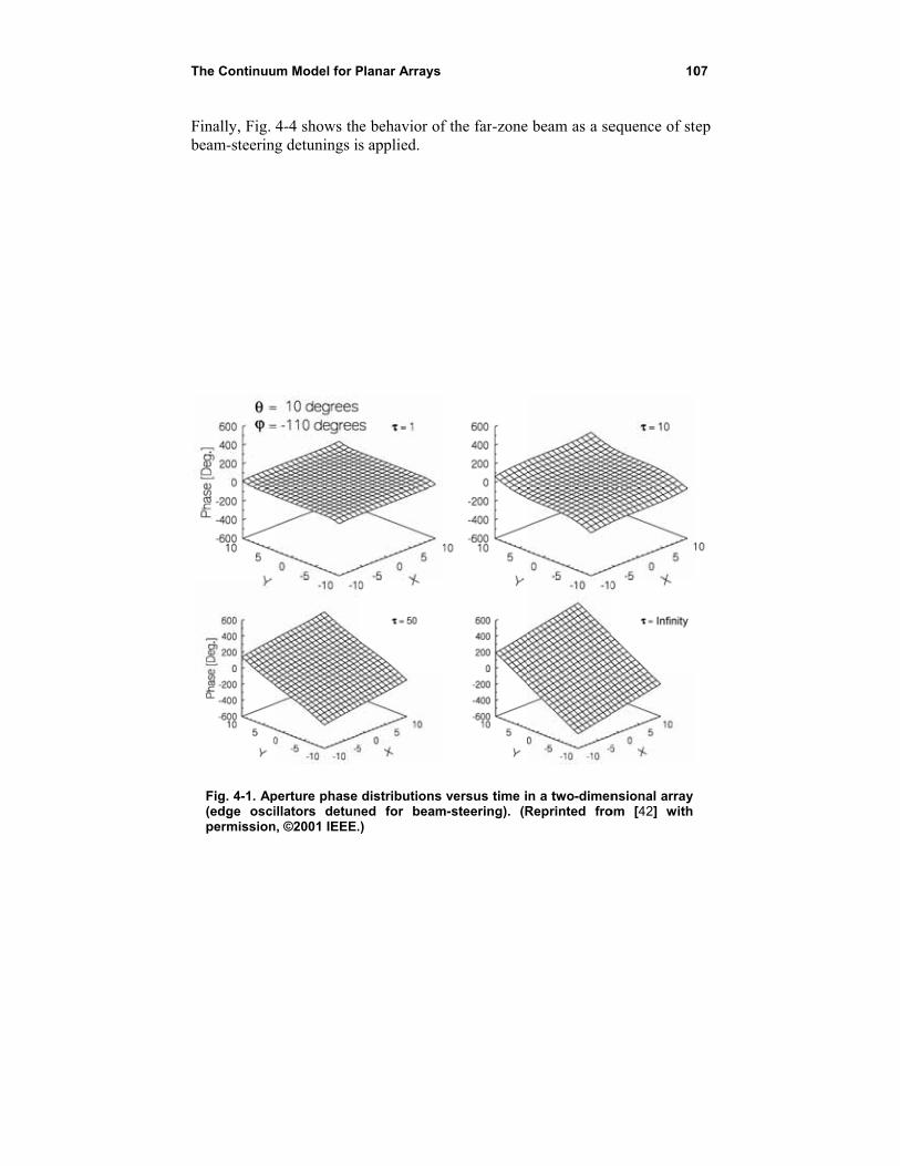
The Continuu
Finally, Fig.beam-steerin
Fig. 4-1. Ap(edge oscipermission
um Model for P
4-4 shows thg detunings i
perture phase illators detun
n, ©2001 IEEE.
Planar Arrays
he behavior ofs applied.
distributions ned for beam.)
f the far-zone
versus time im-steering). (R
e beam as a se
n a two-dimenReprinted fro
10
equence of st
nsional array om [42] with
07
tep
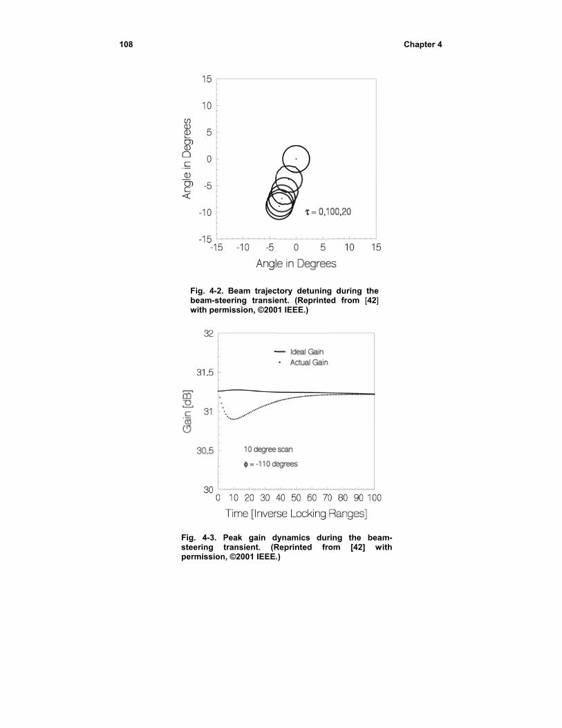
108
Fig. 4-2. beam-stewith perm
Fig. 4-3. Psteering tpermission
Beam trajeceering transiemission, ©200
Peak gain dtransient. (R
n, ©2001 IEEE.
ctory detuningent. (Reprinte01 IEEE.)
dynamics durReprinted fro.)
g during the ed from [42]
ring the beaom [42] w
Chapter
am-with
r 4
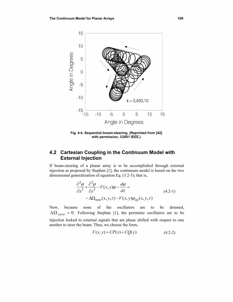
The Continuu
F
4.2 CarteExte
If beam-steeinjection as pdimensional
Now, beca
tune
injection lockanother to ste
um Model for P
Fig. 4-4. Sequw
esian Cournal Inject
ering of a plproposed by Sgeneralization
2 2
2x y
ause none 0 . Followin
ked to externeer the beam.
V
Planar Arrays
ential bream-swith permissio
upling in ttion
lanar array iStephan [1], tn of equation
2
2( , )
( , , )tune
V x yy
x y
of the g Stephan [
nal signals thThus, we cho
( , )V x y CP
steering. (Repon, ©2001 IEE
he Contin
s to be accothe continuum
n Eq. (3.2-3); t
) ( , ) in
d
d
V x y
oscillators 1], the perim
hat are phase oose the form
( ) ( )P x CQ y
printed from [4E.)
nuum Mod
omplished thm model is bathat is,
( , , )nj x y
are to meter oscillat
shifted with m,
10
42]
del with
hrough externased on the tw
(4.2-1)
be detuneators are to b
respect to on
(4.2-2)
09
nal wo
ed, be
ne
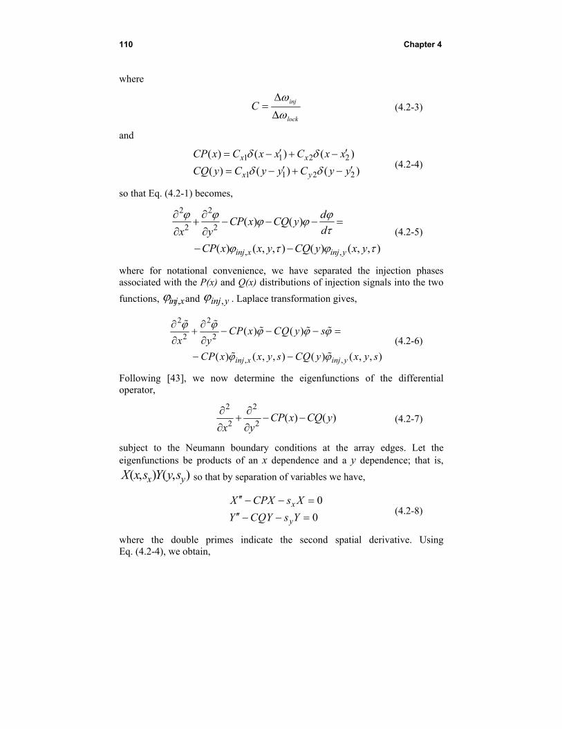
110 Chapter 4
where
lock
injC
(4.2-3)
and
1 1 2 2
1 1 2 2
( ) ( ) ( )
( ) ( ) ( )x x
x y
CP x C x x C x x
CQ y C y y C y y
(4.2-4)
so that Eq. (4.2-1) becomes,
2 2
2 2
, ,
( ) ( )
( ) ( , , ) ( ) ( , , )inj x inj y
dCP x CQ y
dx y
CP x x y CQ y x y
(4.2-5)
where for notational convenience, we have separated the injection phases associated with the P(x) and Q(x) distributions of injection signals into the two
functions, ,inj x and ,inj y . Laplace transformation gives,
2 2
2 2
, ,
( ) ( )
( ) ( , , ) ( ) ( , , )inj x inj y
CP x CQ y sx y
CP x x y s CQ y x y s
(4.2-6)
Following [43], we now determine the eigenfunctions of the differential operator,
2 2
2 2( ) ( )CP x CQ y
x y
(4.2-7)
subject to the Neumann boundary conditions at the array edges. Let the eigenfunctions be products of an x dependence and a y dependence; that is,
( , ) ( , )x yX x s Y y s so that by separation of variables we have,
0
0x
y
X CPX s X
Y CQY s Y
(4.2-8)
where the double primes indicate the second spatial derivative. Using Eq. (4.2-4), we obtain,
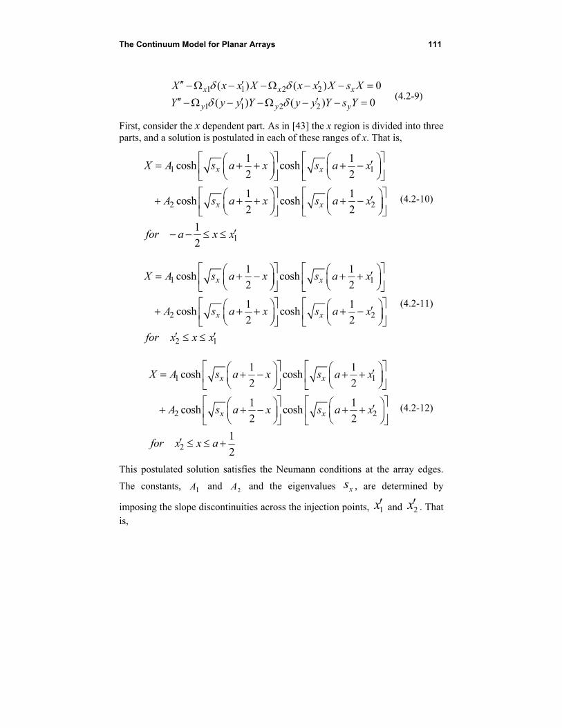
The Continuum Model for Planar Arrays 111
1 1 2 2
1 1 2 2
( ) ( ) 0
( ) ( ) 0x x x
y y y
X x x X x x X s X
Y y y Y y y Y s Y
(4.2-9)
First, consider the x dependent part. As in [43] the x region is divided into three parts, and a solution is postulated in each of these ranges of x. That is,
1 1
2 2
1
1 1cosh cosh
2 2
1 1cosh cosh
2 2
1
2
x x
x x
X A s a x s a x
A s a x s a x
for a x x
(4.2-10)
1 1
2 2
2 1
1 1cosh cosh
2 2
1 1cosh cosh
2 2
x x
x x
X A s a x s a x
A s a x s a x
for x x x
(4.2-11)
1 1
2 2
2
1 1cosh cosh
2 2
1 1cosh cosh
2 2
1
2
x x
x x
X A s a x s a x
A s a x s a x
for x x a
(4.2-12)
This postulated solution satisfies the Neumann conditions at the array edges.
The constants, 1A and 2A and the eigenvalues xs , are determined by
imposing the slope discontinuities across the injection points, 1x and 2x . That is,
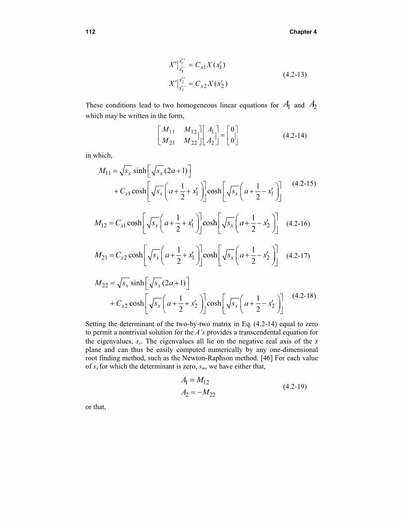
112 Chapter 4
1
11
2
2
1 1
2 2
( )
( )
xxx
xxx
X C X x
X C X x
(4.2-13)
These conditions lead to two homogeneous linear equations for 1A and 2A
which may be written in the form,
11 12 1
21 22 2
0
0
M M A
M M A
(4.2-14)
in which,
11
1 1 1
sinh (2 1)
1 1cosh cosh
2 2
x x
x x x
M s s a
C s a x s a x
(4.2-15)
12 1 1 21 1
cosh cosh2 2x x xM C s a x s a x
(4.2-16)
21 2 1 21 1
cosh cosh2 2x x xM C s a x s a x
(4.2-17)
22
2 2 2
sinh (2 1)
1 1cosh cosh
2 2
x x
x x x
M s s a
C s a x s a x
(4.2-18)
Setting the determinant of the two-by-two matrix in Eq. (4.2-14) equal to zero to permit a nontrivial solution for the A’s provides a transcendental equation for the eigenvalues, sx. The eigenvalues all lie on the negative real axis of the s plane and can thus be easily computed numerically by any one-dimensional root finding method, such as the Newton-Raphson method. [46] For each value of sx for which the determinant is zero, sm, we have either that,
1 12
2 22
A M
A M
(4.2-19)
or that,
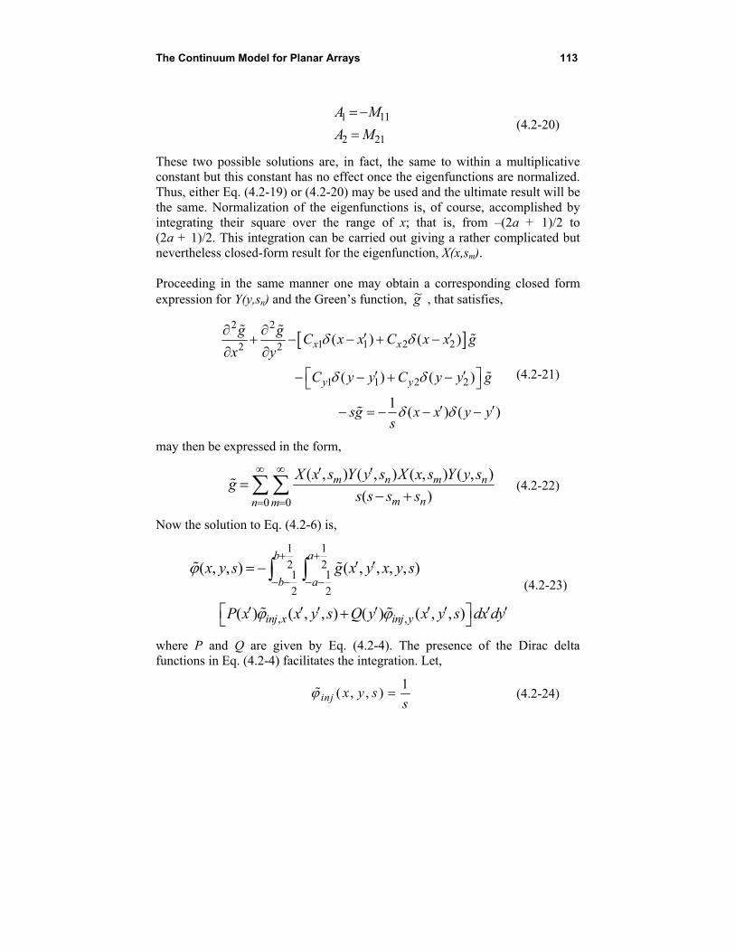
The Continuum Model for Planar Arrays 113
1 11
2 21
A M
A M
(4.2-20)
These two possible solutions are, in fact, the same to within a multiplicative constant but this constant has no effect once the eigenfunctions are normalized. Thus, either Eq. (4.2-19) or (4.2-20) may be used and the ultimate result will be the same. Normalization of the eigenfunctions is, of course, accomplished by integrating their square over the range of x; that is, from –(2a + 1)/2 to (2a + 1)/2. This integration can be carried out giving a rather complicated but nevertheless closed-form result for the eigenfunction, X(x,sm). Proceeding in the same manner one may obtain a corresponding closed form expression for Y(y,sn) and the Green’s function, g~ , that satisfies,
2 2
1 1 2 22 2
1 1 2 2
( ) ( )
( ) ( )
1( ) ( )
x x
y y
g gC x x C x x g
x y
C y y C y y g
sg x x y ys
(4.2-21)
may then be expressed in the form,
0 0
( , ) ( , ) ( , ) ( , )
( )m n m n
m nn m
X x s Y y s X x s Y y sg
s s s s
(4.2-22)
Now the solution to Eq. (4.2-6) is,
1 1
2 21 1
2 2
, ,
( , , ) ( , , , , )
( ) ( , , ) ( ) ( , , )
b a
b a
inj x inj y
x y s g x y x y s
P x x y s Q y x y s dx dy
(4.2-23)
where P and Q are given by Eq. (4.2-4). The presence of the Dirac delta functions in Eq. (4.2-4) facilitates the integration. Let,
1
( , , )inj x y ss
(4.2-24)
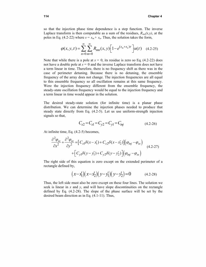
114 Chapter 4
so that the injection phase time dependence is a step function. The inverse Laplace transform is then computable as a sum of the residues, Rmn(x,y), at the poles in Eq. (4.2-22) where s = sm + sn. Thus, the solution takes the form,
( )
0 0
( , , ) ( , ) 1 ( )m ns smn
n m
x y R x y e u
(4.2-25)
Note that while there is a pole at s = 0, its residue is zero so Eq. (4.2-22) does not have a double pole at s = 0 and the inverse Laplace transform does not have a term linear in time. Therefore, there is no frequency shift as there was in the case of perimeter detuning. Because there is no detuning, the ensemble frequency of the array does not change. The injection frequencies are all equal to this ensemble frequency so all oscillation remains at this same frequency. Were the injection frequency different from the ensemble frequency, the steady-state oscillation frequency would be equal to the injection frequency and a term linear in time would appear in the solution. The desired steady-state solution (for infinite time) is a planar phase distribution. We can determine the injection phases needed to produce that steady state directly from Eq. (4.2-5). Let us use uniform-strength injection signals so that,
2 1 2 1x x y y injC C C C C (4.2-26)
At infinite time, Eq. (4.2-5) becomes,
2 2
1 1 2 22 2
1 1 2 2
( ) ( )
( ) ( )
ss ssx x inj ss
y y inj ss
C x x C x xx y
C y y C y y
(4.2-27)
The right side of this equation is zero except on the extended perimeter of a rectangle defined by,
1 2 1 2 0x x x x y y y y (4.2-28)
Thus, the left side must also be zero except on these four lines. The solution we seek is linear in x and y, and will have slope discontinuities on the rectangle defined by Eq. (4.2-28). The slope of the phase surface will be set by the desired beam direction as in Eq. (4.1-11). Thus,
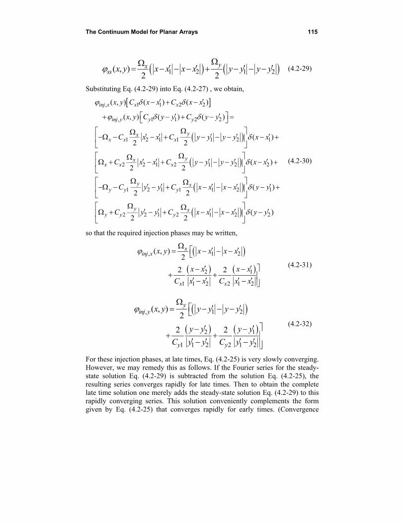
The Continuum Model for Planar Arrays 115
1 2 1 2( , )2 2
yxss x y x x x x y y y y
(4.2-29)
Substituting Eq. (4.2-29) into Eq. (4.2-27) , we obtain,
, 1 1 2 2
, 1 1 2 2
1 2 1 1 1 2 1
2 2 1 2 1 2 2
1 2 1 1
( , ) ( ) ( )
( , ) ( ) ( )
( )2 2
( )2 2
2 2
inj x x x
inj y y y
yxx x x
yxx x x
y xy y y
x y C x x C x x
x y C y y C y y
C x x C y y y y x x
C x x C y y y y x x
C y y C x
1 2 1
2 2 1 2 1 2 2
( )
( )2 2
y xy y y
x x x y y
C y y C x x x x y y
(4.2-30)
so that the required injection phases may be written,
, 1 2
2 1
1 1 2 2 1 2
( , )2
2 2
xinj x
x x
x y x x x x
x x x x
C x x C x x
(4.2-31)
, 1 2
2 1
1 1 2 2 1 2
( , )2
2 2
yinj y
y y
x y y y y y
y y y y
C y y C y y
(4.2-32)
For these injection phases, at late times, Eq. (4.2-25) is very slowly converging. However, we may remedy this as follows. If the Fourier series for the steady-state solution Eq. (4.2-29) is subtracted from the solution Eq. (4.2-25), the resulting series converges rapidly for late times. Then to obtain the complete late time solution one merely adds the steady-state solution Eq. (4.2-29) to this rapidly converging series. This solution conveniently complements the form given by Eq. (4.2-25) that converges rapidly for early times. (Convergence
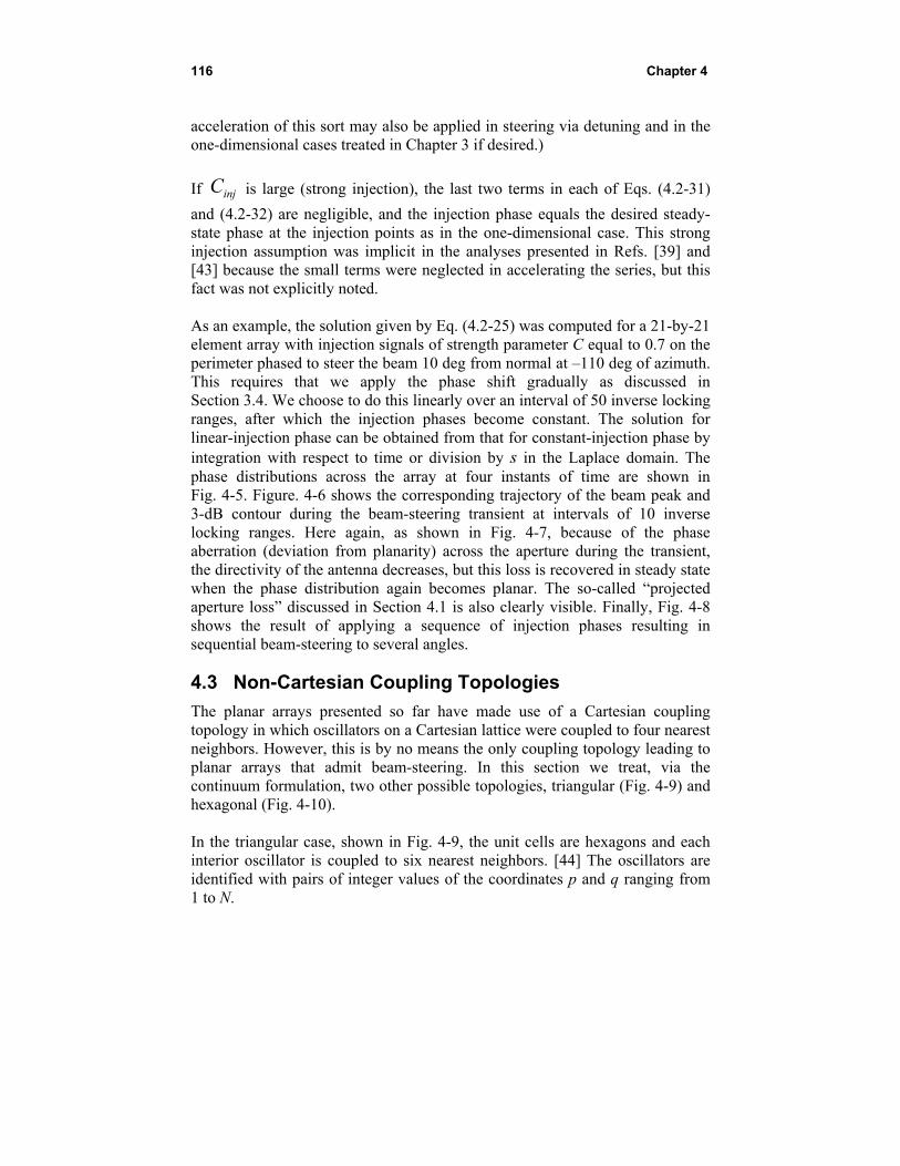
116 Chapter 4
acceleration of this sort may also be applied in steering via detuning and in the one-dimensional cases treated in Chapter 3 if desired.)
If injC is large (strong injection), the last two terms in each of Eqs. (4.2-31)
and (4.2-32) are negligible, and the injection phase equals the desired steady-state phase at the injection points as in the one-dimensional case. This strong injection assumption was implicit in the analyses presented in Refs. [39] and [43] because the small terms were neglected in accelerating the series, but this fact was not explicitly noted. As an example, the solution given by Eq. (4.2-25) was computed for a 21-by-21 element array with injection signals of strength parameter C equal to 0.7 on the perimeter phased to steer the beam 10 deg from normal at –110 deg of azimuth. This requires that we apply the phase shift gradually as discussed in Section 3.4. We choose to do this linearly over an interval of 50 inverse locking ranges, after which the injection phases become constant. The solution for linear-injection phase can be obtained from that for constant-injection phase by integration with respect to time or division by s in the Laplace domain. The phase distributions across the array at four instants of time are shown in Fig. 4-5. Figure. 4-6 shows the corresponding trajectory of the beam peak and 3-dB contour during the beam-steering transient at intervals of 10 inverse locking ranges. Here again, as shown in Fig. 4-7, because of the phase aberration (deviation from planarity) across the aperture during the transient, the directivity of the antenna decreases, but this loss is recovered in steady state when the phase distribution again becomes planar. The so-called “projected aperture loss” discussed in Section 4.1 is also clearly visible. Finally, Fig. 4-8 shows the result of applying a sequence of injection phases resulting in sequential beam-steering to several angles.
4.3 Non-Cartesian Coupling Topologies
The planar arrays presented so far have made use of a Cartesian coupling topology in which oscillators on a Cartesian lattice were coupled to four nearest neighbors. However, this is by no means the only coupling topology leading to planar arrays that admit beam-steering. In this section we treat, via the continuum formulation, two other possible topologies, triangular (Fig. 4-9) and hexagonal (Fig. 4-10). In the triangular case, shown in Fig. 4-9, the unit cells are hexagons and each interior oscillator is coupled to six nearest neighbors. [44] The oscillators are identified with pairs of integer values of the coordinates p and q ranging from 1 to N.
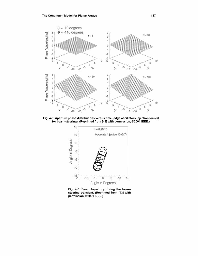
The Continuu
Fig. 4-5. Apefor bea
um Model for P
rture phase dam-steering).
Fig. 4-6steeringpermiss
Planar Arrays
istributions ve(Reprinted fro
6. Beam trajecg transient. (Rsion, ©2001 IE
ersus time (edom [43] with p
ctory during Reprinted fromEE.)
dge oscillatorspermission, ©2
the beam-m [43] with
11
s injection loc2001 IEEE.)
17
cked
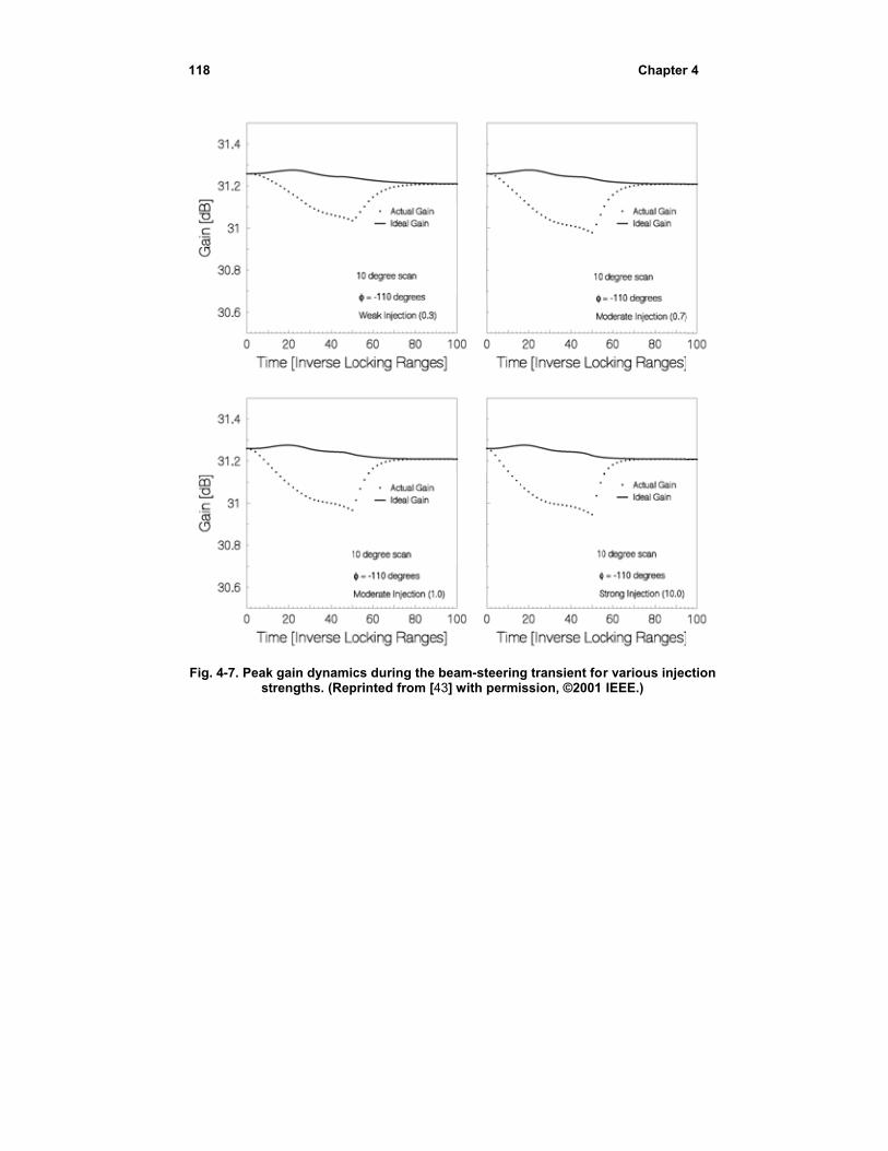
118
Fig. 4-7. Peakst
k gain dynamictrengths. (Rep
cs during the printed from [4
beam-steerin43] with permi
g transient foission, ©2001
Chapter
r various injecIEEE.)
r 4
ction
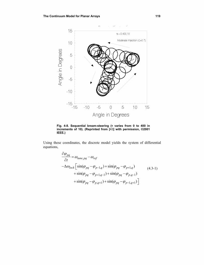
The Continuum Model for Planar Arrays 119
Fig. 4-8. Sequential bream-steering (τ varies from 0 to 400 in increments of 10). (Reprinted from [43] with permission, ©2001 IEEE.)
Using these coordinates, the discrete model yields the system of differential equations,
,
1, 1,
1, 1 , 1
, 1 1, 1
sin( ) sin( )
sin( ) sin( )
sin( ) sin( )
pqtune pq ref
lock pq p q pq p q
pq p q pq p q
pq p q pq p q
t
(4.3-1)

120 Chapter 4
Fig. 4-9. Oscillators coupled on an equilateral triangular lattice. (Reprinted with
permission from [44], ©2004 IEEE.)
Fig. 4-10. Oscillators coupled on a hexagonal lattice. (Reprinted with permission
from [44], ©2004 IEEE.)
X
Y
a
(N-1)a
p
q
X
Y
a
(N-1)a
p
q
X
Y
a
(N-1)a
p
q
X
Y
a
(N-1)a
p
q
X
Y
a
(N-1)a
a
(N-1)a
p
q
X
Y
a
(N-1)a
p
q
X
Y
a
(N-1)a
p
q
X
Y
a
(N-1)a
p
q
X
Y
a
(N-1)a
a
(N-1)a
p
q
X
Y
a
(N-1)a
a
(N-1)a
p
q
X
Y
a
(N-1)a
p
q
X
Y
a
(N-1)a
1
(N-1)a
p
q
X
Y
(N-1)a(N-1)a
p
q
(N-1)a(N-
p
q
N
x
y
X
Y
a
(N-1)a
p
q
X
Y
a
(N-1)a
p
q
X
Y
a
(N-1)a
p
q
X
Y
a
(N-1)a
p
q
X
Y
a
(N-1)a
a
(N-1)a
p
q
X
Y
a
(N-1)a
p
q
X
Y
a
(N-1)a
p
q
X
Y
a
(N-1)a
p
q
X
Y
a
(N-1)a
a
(N-1)a
p
q
X
Y
a
(N-1)a
a
(N-1)a
p
q
X
Y
a
(N-1)a
p
q
X
Y
a
(N-1)a
1
(N-1)a
p
q
X
Y
(N-1)a(N-1)a
p
q
(N-1)a(N-
p
q
N
X
Y
a
(N-1)a
p
q
X
Y
a
(N-1)a
p
q
X
Y
a
(N-1)a
p
q
X
Y
a
(N-1)a
a
(N-1)a
p
q
X
Y
a
(N-1)a
a
(N-1)a
p
q
X
Y
a
(N-1)a
p
q
X
Y
a
(N-1)a
a
(N-1)a
p
q
X
Y
a
(N-1)a
a
(N-1)a
p
q
X
Y
a
(N-1)a
a
(N-1)a
p
q
X
Y
a
(N-1)a
p
q
X
Y
a
(N-1)a
p
q
X
Y
a
(N-1)a
a
(N-1)a
p
q
X
Y
a
(N-1)a
p
q
X
Y
a
(N-1)a
a
(N-1)a
p
q
X
Y
a
(N-1)a
a
(N-1)a
p
q
X
Y
a
(N-1)a
a
(N-1)a
p
q
X
Y
a
(N-1)a
a
(N-1)a
p
q
X
Y
a
(N-1)a
a
(N-1)a
p
q
X
Y
a
(N-1)a
1
(N-1)a
p
q
X
Y
(N-1)a(N-1)a
p
q
(N-1)a(N-
p
q
N
x
y
x
y
1
N
p
q
32
13
1
x
y
1
N
p
q
32
13
1
x
y
1
N
p
q
32
13
1
The Continuum Model for Planar Arrays 121
where we have assumed that the coupling phases are multiples of 2π. We remark that this system of nonlinear equations can be solved numerically to yield the full nonlinear solution for the dynamic behavior of the phase distribution. However, as mentioned earlier, the analytic solution of the linearized formulation provides more insight. Linearizing and expanding in Taylor series to second order leads to,
2 2 2
2 22 ( , )tune p q
p qp q
(4.3-2)
where, as before, lockt and ( ) /tune tune ref lock .
Transforming to Cartesian coordinates, x and y, we arrive at,
2 2
2 2
1
3tune
triTx y
(4.3-3)
and Ttri = (3/2)τ. This equation is very much like Eq. (4.1-2) for the Cartesian case except for the scaling of the time and the detuning. In the hexagonal case, shown in Fig. 4-10, the unit cells ar triangular and each interior oscillator is coupled to three nearest neighbors [44]. Following a procedure analogous to that presented above for the triangular case leads to,
2 2
2 23 tune
hexTx y
(4.3-4)
and Thex = τ/4. Again, this equation is very much like Eq. (4.1-2) for the Cartesian case except for the scaling of the time and the detuning. Finite arrays using the triangular and hexagonal coupling schemes may be constructed with equilateral triangular boundaries, and the boundary conditions on the phase will again be of the Neumann type. Just as was the case for rectangular arrays, if the oscillators on the triangular boundary are detuned, the steady-state interior phases are governed by Laplace’s equation, and planar distributions are an obtainable special case. The desired steady-state solution to produce a beam steered to spherical coordinate angles, 0 0( , ) , is,
0 0 0 02
( , , ) sin cos sin sin3
d Nx y x y
(4.3-5)
122 Chapter 4
where d is the separation of the radiating elements in the y coordinate for fixed x, and is the wavelength. Substituting this desired steady-state phase distribution, Eq. (4.3-5), into the partial differential equations, Eqs. (4.3-3) and (4.3-4), gives the required detuning of the perimeter oscillators.
0 03
0 03
0 03/2
2 2sin cos
3
2 2sin cos
3
2sin cos
tune x y
tune x y
tune x A
d
d
d
(4.3-6)
where A is the length of a side of the array, Nd , and is 1/ 3 for the
triangular coupling and 3 for hexagonal coupling. Note that the sum of these detunings is zero for all steering angles so that the ensemble frequency of the array is unchanged. At this point we note for later reference that it is possible to obtain the needed tuning for a given planar steady-state phase distribution from the full nonlinear formulation Eq. (4.3-1). Inserting the desired phase Eq. (4.3-5) into Eq. (4.3-1) and evaluating on the boundary of the triangle we obtain,
0 03
0 0
0 03
0 0
0 03/2
1 2sin sin cos
63
1 2sin sin cos
23
1 2sin sin cos
63
1 2sin sin cos
23
1 2 5sin sin cos
3
tune x y
tune x y
tune x A
d
d
d
d
d
0 0
6
1 2 5sin sin cos
63
d
(4.3-7)

The Continuum Model for Planar Arrays 123
which reduces to Eq. (4.3-6) for small θ0;. that is, for small inter-oscillator phase differences when the linearization is accurate. Note that the sum of these detunings is exactly zero regardless of steering angle. We propose that the solutions of the partial differential equations, Eq. (4.3-3) and Eq. (4.3-4), be obtained as series of the eigenfunctions of the differential operators subject to Neumann boundary conditions on the triangular boundary of the arrays. These eigenfunctions have been studied in the context of waveguides of triangular cross section and are thus well known. They are expressed as sums of three products of two of the trigonometric functions, sine and cosine. These eigenfunctions and their useful properties are summarized in the appendix of Ref. [44]. We wish to solve,
2 2
2 2 tuneTx y
(4.3-8)
with the detuning function given by Eq. (4.3-6), and we will assume that the detuning is a step function in time. Laplace transformation of Eq. (4.3-8) gives,
2 2
2 2( , )tune tunes x y
sx y
(4.3-9)
The solution will be of the form,
( )( , , ) ( , ) 1 ( )mnTimn mn
mn
x y C H x y e u T (4.3-10)
where the H functions are the normalized eigenfunctions on the triangle with the superscript denoting even or odd symmetry of the function in y. Thus, the unknown coefficients may be found from the desired steady-state phase distribution, Eq. (4.3-5), by setting T to infinity in Eq. (4.3-10) and setting the resulting sum equal to the steady-state solution. Then, the orthogonality of the eigenfunctions permits us to find the coefficients, Cmn. This procedure is completely equivalent to expressing the Green’s function as a sum of the eigenfunctions and then integrating the product of the Green’s function and the desired steady-state phase distribution as was done in the Cartesian case. As was done in Ref. [44], we now provide a number of computed examples demonstrating the dynamic behavior obtained via the various formulations of the problem; that is, the nonlinear model, the linearized discrete model, and the continuum model for both the triangular and hexagonal coupling topologies.
124 Chapter 4
We begin with triangular coupling with N = 28 resulting in a 435-oscillator array. We completely preclude the appearance of grating lobes in the visible region by selecting the radiating element spacing, d, to be / 3 . We note, however, that, because the maximum permissible phase difference between
coupled oscillators is 90 deg, the element spacing can be as large as 3/2 without the appearance of visible grating lobes. The array size, A, in the continuum model is taken to be ( 1)( 2)d N N instead of Nd because that makes
the array area equal to the sum of the unit cell areas, resulting in a more accurate directivity. Figure 4-11 shows the aperture phase distribution for four instants of time computed using the continuum model with perimeter detuning given by Eq. (4.3-6) and unit step temporal dependence and steady-state beam-pointing angles θ0, φ0) = 10 deg, 45 deg). Note the rather severe phase aberration at time equal to 10 inverse locking ranges. Figure 4-12 shows the directivity (gain in the absence of loss) computed by pattern integration as a function of time during the beam-steering transient. The solid curve is the result of planar phase distribution, and “projected aperture loss” is again evident. In the left plot, the continuum result is compared with the full nonlinear solution obtained numerically, and in the right plot the numerical solution of the linearized discrete model is compared with the nonlinear solution. Note that the dip in gain at about 10 inverse locking ranges correlates with the severe aberration at that time in Fig. 4-11. The nonlinear solution used Eq. (4.3-7) while the linear ones used Eq. (4.3-6) as detuning. Because the angle from normal is only 10 deg, the error in the linear approximation of the sine functions is less than 6.5 percent, and the linearized and continuum results agree well with the full nonlinear result taken to be the correct behavior. Figure 4-13 shows the trajectory of the beam peak and 3-dB contour during the beam-steering transient as computed via the three formulations, and, as should be expected for this small steering angle, they agree very well. Now, if the final beam angle is increased from 10 deg to 25 deg, the error in the linear approximation of the sine function is almost 49 percent, and the discrepancy between the linear and nonlinear results in Fig. 4-14 show the impact of this in that the gain error at the dip is about 2 dB, and the curves are slightly different in shape. However, there is still qualitative agreement between the linear and nonlinear results.
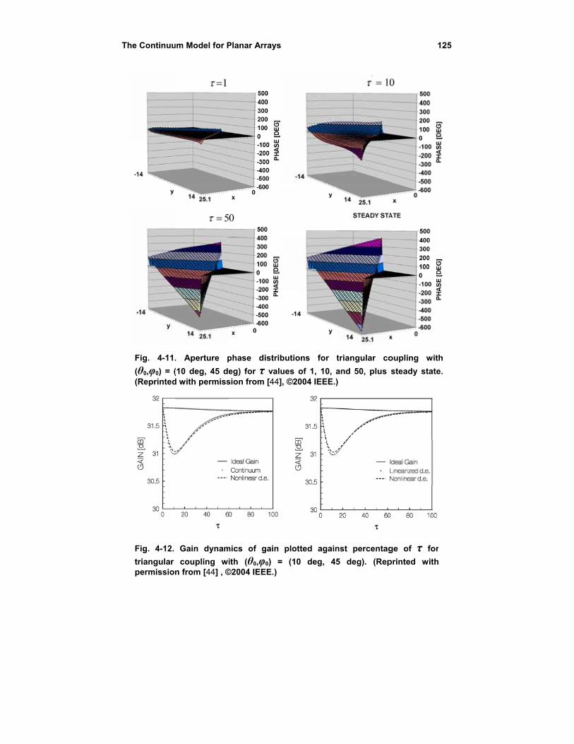
The Continuu
Fig. 4-11.
(θ0,φ0) = ((Reprinted
Fig. 4-12.
triangular permissio
um Model for P
. Aperture p
(10 deg, 45 ded with permiss
Gain dynam
coupling win from [44] , ©
Planar Arrays
phase distrib
eg) for τ valusion from [44],
mics of gain
ith (θ0,φ0) =©2004 IEEE.)
butions for
ues of 1, 10, a, ©2004 IEEE.)
plotted again
(10 deg, 45
triangular co
and 50, plus )
nst percentag
5 deg). (Rep
12
oupling with
steady state.
ge of τ for
printed with
25
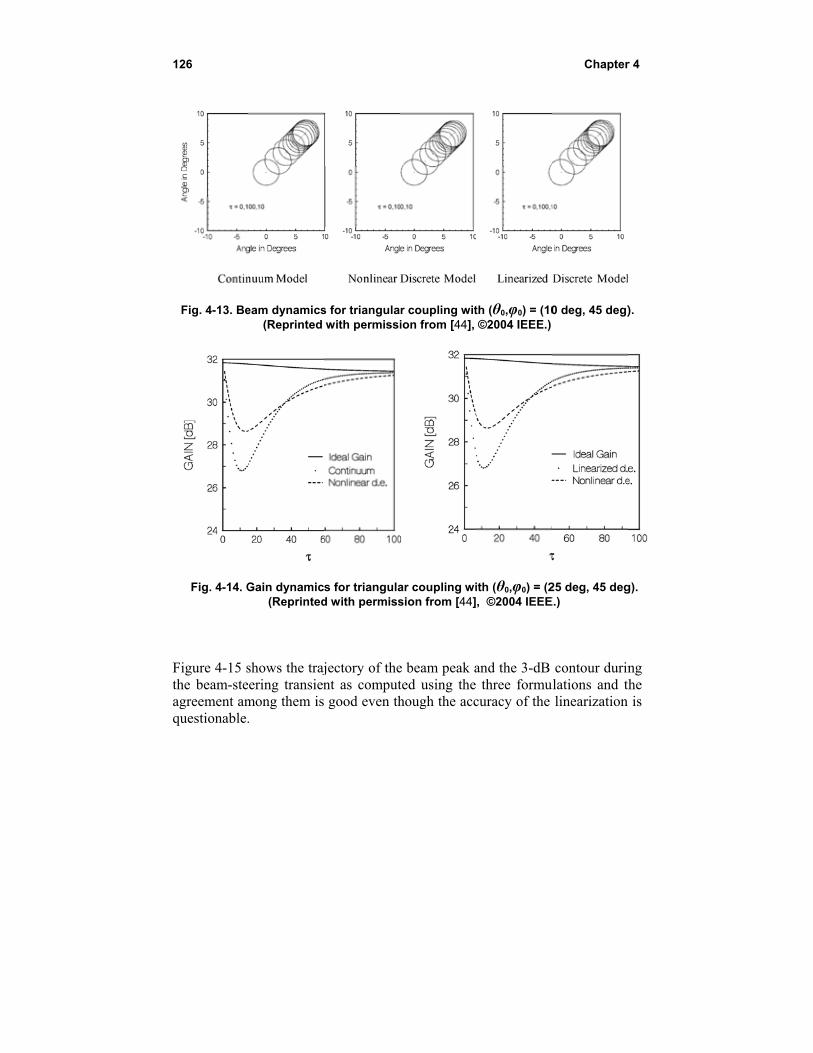
126
Fig. 4-13. Be
Fig. 4-14. G
Figure 4-15 sthe beam-steagreement amquestionable.
eam dynamics(Reprinted
Gain dynamic(Reprinted
shows the trajeering transienmong them is.
s for triangulawith permissi
s for triangulad with permiss
jectory of thent as comput good even th
r coupling wition from [44],
ar coupling wision from [44]
e beam peak ated using thehough the acc
th (θ0,φ0) = (10©2004 IEEE.)
ith (θ0,φ0) = (2, ©2004 IEEE
and the 3-dB three formucuracy of the
Chapter
0 deg, 45 deg)
25 deg, 45 degE.)
contour durinulations and th
linearization
r 4
).
g).
ng the is
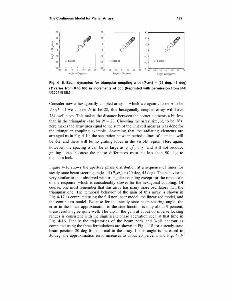
The Continuu
Fig. 4-15. Be
(τ varies from©2004 IEEE.)
Consider now
/ 3 . If w
784 oscillatorthan in the trhere makes ththe triangulaarranged as ibe λ/2, and t
however, thegrating lobemaintain lock Figure 4-16 steady-state bvery similar of the responcourse, one mtriangular onFig. 4-17 as cthe continuuerror in the lthese results ranges is conFig. 4-16. Fcomputed usibeam positio30 deg, the a
um Model for P
am dynamics
m 0 to 600 in
w a hexagona
we choose N
rs. This makeriangular casehe array area ar coupling ein Fig. 4-10, tthere will be
e spacing d cs because thk.
shows the apbeam-steeringto that observnse, which ismust remembne. The tempcomputed usim model. Belinear approxagree quite w
nsistent with Finally the tring the three
on 20 deg froapproximation
Planar Arrays
s for triangula
increments o
ally coupled
to be 28, th
es the distance for N = 28equal to the s
example. Assthe separatione no grating
can be as larhe phase diff
perture phaseg angles of (θved with trian considerably
ber that this aporal behavioing the full noecause for th
ximation to thwell. The dipthe significa
rajectories offormulations
om normal ton error incre
ar coupling w
of 50.) (Reprin
array in whic
his hexagonal
ce between th8. Choosing thsum of the unsuming that n between perlobes in the
rge as 3fferences mus
e distribution θ0,φ0) = (20 dngular coupliy slower for array has manor of the gainonlinear modehis steady-stahe sine functip in the gain ant phase abef the beam pare shown in
o the array. Iases to about
with (θ0,φ0) =
nted with perm
ch we again
lly coupled a
he corner elemhe array size
nit cell areas athe radiatingriodic lines ovisible regio
/ 2 and stist be less th
at a sequencdeg, 45 deg). Tng except forthe hexagonany more osciln of this arrael, the linearizte beam-steerion is only abat about 60 i
erration seen peak and 3-n Fig. 4-18 foIf this angle t 20 percent,
12
(25 deg, 45 d
mission from
choose d to b
array will hav
ments a bit lee, A, to be Nas was done fg elements aof elements won. Here agai
ill not produhan 90 deg
ce of times fThe behavior r the time scaal coupling. Ollators than tay is shown zed model, anring angle, tbout 9 perceninverse lockinat that time dB contour
or a steady-stais increased
, and Fig. 4-
27
deg).
[44],
be
ave
ess Nd for are
will in,
uce to
for r is ale Of the in nd the nt, ng in as
ate to 19
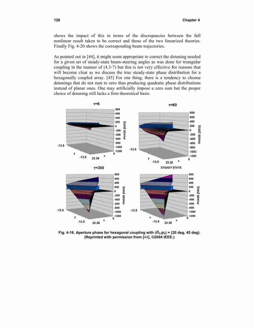
128
shows the inonlinear resFinally Fig. 4 As pointed oufor a given scoupling in twill become hexagonally detunings thainstead of plchoice of det
Fig. 4-16. A
mpact of thsult taken to 4-20 shows th
ut in [44], it mset of steady-the manner of
clear as we coupled arra
at do not sumanar ones. Ontuning still lac
Aperture phase(Reprinted
is in terms be correct a
he correspond
might seem apstate beam-stf (4.3-7) but tdiscuss the t
ay. [45] For om to zero thusne may artificks a firm the
e for hexagond with permiss
of the discrand those of ding beam traj
ppropriate to teering anglesthis is not vetrue steady-stone thing, thes producing qicially imposeeoretical basis
nal coupling wsion from [44]
repancies betthe two lineajectories.
correct the ds as was done
ery effective ftate phase disere is a tendequadratic phase a zero sum s.
with (θ0,φ0) = (2], ©2004 IEEE.
Chapter
tween the fuarized theorie
detuning neede for triangulfor reasons thstribution forency to choose distributiobut the prop
20 deg, 45 deg.)
r 4
ull es.
ded lar hat r a ose ons per
g).
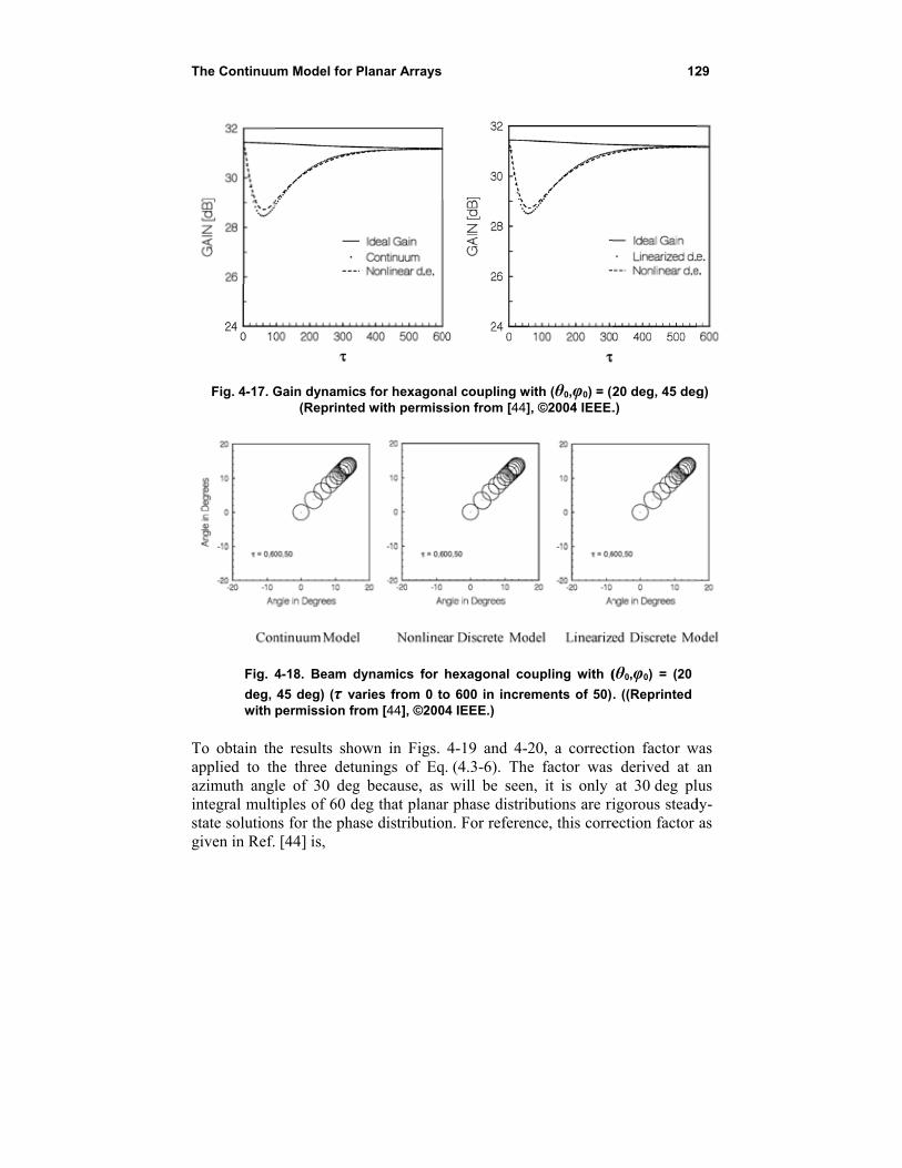
The Continuu
Fig. 4-17. G
Fig. 4
deg, with
To obtain thapplied to thazimuth anglintegral multstate solutiongiven in Ref.
um Model for P
Gain dynamic(Reprinted
4-18. Beam d
45 deg) (τ vapermission fro
he results shohe three detule of 30 degtiples of 60 dens for the pha [44] is,
Planar Arrays
s for hexagond with permiss
dynamics for
aries from 0 toom [44], ©200
own in Figs. unings of Eqg because, aseg that planar
ase distributio
nal coupling wsion from [44]
hexagonal co
o 600 in incre04 IEEE.)
4-19 and 4-2q. (4.3-6). The
will be seenr phase distri
on. For referen
with (θ0,φ0) = (2], ©2004 IEEE.
oupling with (
ements of 50)
20, a correcte factor wasn, it is only butions are rince, this corre
12
20 deg, 45 deg.)
(θ0,φ0) = (20
. ((Reprinted
tion factor ws derived at
at 30 deg pligorous steadection factor
29
g)
was an lus dy-as
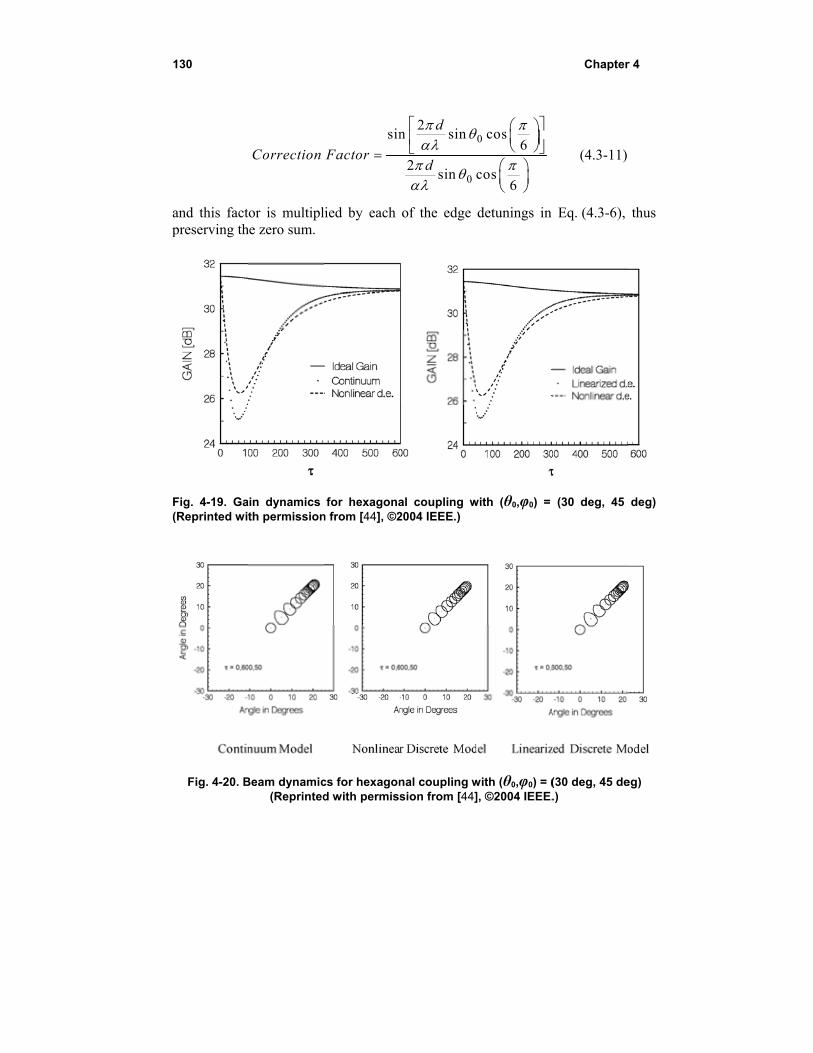
130
and this factpreserving th
Fig. 4-19. Ga(Reprinted wi
Fig. 4-20. B
Correction
tor is multiplhe zero sum.
ain dynamics th permission
Beam dynamic(Reprinted
sin
Factor
lied by each
for hexagonan from [44], ©2
cs for hexagond with permiss
0
2n sin
2sin
d
d
of the edge
al coupling w2004 IEEE.)
nal coupling wsion from [44]
0 cos6
cos6
detunings in
with (θ0,φ0) =
with (θ0,φ0) = (], ©2004 IEEE.
Chapter
(4.3-11)
Eq. (4.3-6),
(30 deg, 45
(30 deg, 45 de.)
r 4
thus
deg)
eg)
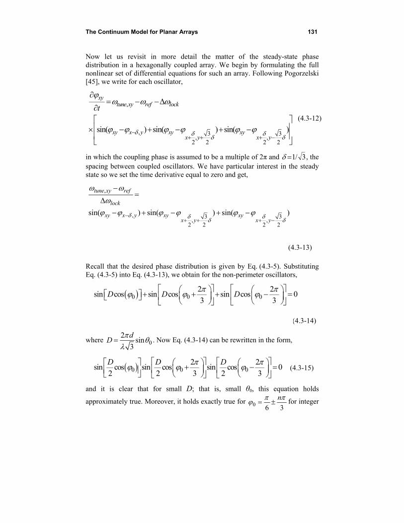
The Continuum Model for Planar Arrays 131
Now let us revisit in more detail the matter of the steady-state phase distribution in a hexagonally coupled array. We begin by formulating the full nonlinear set of differential equations for such an array. Following Pogorzelski [45], we write for each oscillator,
,
, 3 3, ,
2 2 2 2
sin( ) sin( ) sin( )
xytune xy ref lock
xy x y xy xyx y x y
t
(4.3-12)
in which the coupling phase is assumed to be a multiple of 2π and 3/1 , the spacing between coupled oscillators. We have particular interest in the steady state so we set the time derivative equal to zero and get,
,
, 3 3, ,
2 2 2 2
sin( ) sin( ) sin( )
tune xy ref
lock
xy x y xy xyx y x y
(4.3-13)
Recall that the desired phase distribution is given by Eq. (4.3-5). Substituting Eq. (4.3-5) into Eq. (4.3-13), we obtain for the non-perimeter oscillators,
0 0 02 2
sin cos sin cos sin cos 03 3
D D D
(4.3-14)
where 02
sin3
dD
. Now Eq. (4.3-14) can be rewritten in the form,
0 0 02 2
sin cos sin cos sin cos 02 2 3 2 3
D D D (4.3-15)
and it is clear that for small D; that is, small θ0, this equation holds
approximately true. Moreover, it holds exactly true for 0 6 3
n for integer
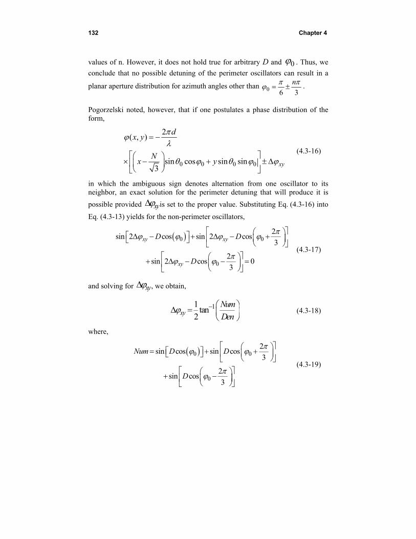
132 Chapter 4
values of n. However, it does not hold true for arbitrary D and 0 . Thus, we
conclude that no possible detuning of the perimeter oscillators can result in a
planar aperture distribution for azimuth angles other than 0 6 3
n .
Pogorzelski noted, however, that if one postulates a phase distribution of the form,
0 0 0 0
2( , )
sin cos sin sin3
xy
dx y
Nx y
(4.3-16)
in which the ambiguous sign denotes alternation from one oscillator to its neighbor, an exact solution for the perimeter detuning that will produce it is
possible provided xy is set to the proper value. Substituting Eq. (4.3-16) into
Eq. (4.3-13) yields for the non-perimeter oscillators,
0 0
0
2sin 2 cos sin 2 cos
3
2sin 2 cos 0
3
xy xy
xy
D D
D
(4.3-17)
and solving for xy , we obtain,
11
tan2xy
Num
Den
(4.3-18)
where,
0 0
0
2sin cos sin cos
3
2sin cos
3
Num D D
D
(4.3-19)
The Continuum Model for Planar Arrays 133
0 0
0
2cos cos cos cos
3
2cos cos
3
Den D D
D
(4.3-20)
Finally substituting Eq. (4.3-16) with Eq. (4.3-18) into Eq. (4.3-13) yields the perimeter detuning required to produce this non-planar phase distribution. The result is,
0 03
0 03
0 0(3 1) 3/6
2 2sin sin cos 2
33
2 2sin sin cos 2
33
2sin sin cos 2
3
tune xyx y
tune xyx y
tune xyx N
d
d
d
(4.3-21)
for the edge elements and
0 0
0 0
0 0
(3 1) 3 ( 1),
6 2
2 2sin sin cos 2
33
(3 1) 3 ( 1),
6 2
2 2sin sin cos 2
33
1 2,0 sin sin cos 2
3 3
tune
xy
tune
xy
tune xy
N N
d
N N
d
d
(4.3-22)
for the corner elements. Because of Eq. (4.3-17), the sum of these detunings is always zero so that the ensemble frequency of the array remains constant. Figure 4-21 shows a typical phase distribution for such an array. Figure 4-21(a) shows the phase distribution, and Fig. 4-21(b) shows the deviation, ±4.67 deg, from planar.
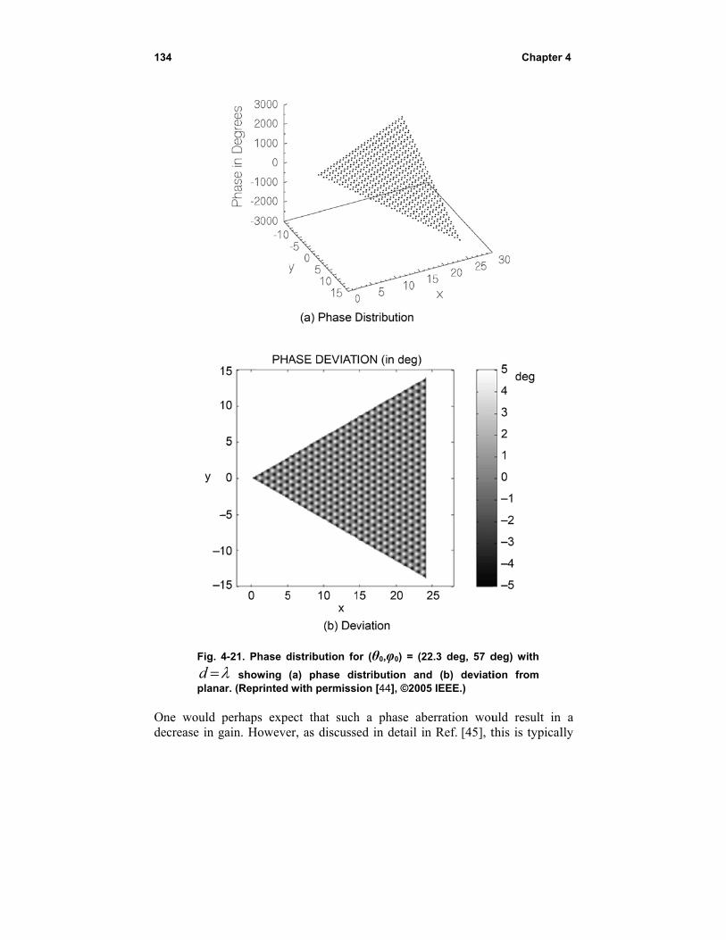
134
Fig. 4
dplana
One would decrease in g
4-21. Phase d
showing ar. (Reprinted
perhaps expegain. Howeve
distribution fo
(a) phase diswith permiss
ect that sucher, as discusse
or (θ0,φ0) = (2
stribution anion [44], ©200
h a phase abed in detail in
22.3 deg, 57 d
nd (b) deviati05 IEEE.)
berration woun Ref. [45], t
Chapter
deg) with
ion from
uld result in this is typical
r 4
a lly
The Continuum Model for Planar Arrays 135
not the case. The power that would have been radiated by a planar phase distribution is partially shifted by the phase alternation into the invisible region. Thus, this part is not radiated, and the power input to the antenna is decreased by the same amount. As a result, the directivity is unaffected by the phase alternation! The only circumstance resulting in a decrease in the gain is when the combination of element spacing and steering angle results in one or more grating lobes in the visible region. Analytical estimation of this effect is discussed in Ref. [45]. Finally, we remark that a planar steady-state phase distribution is of course attainable if one is willing to detune all of the oscillators in the hexagonally coupled array. This would require that alternate oscillators be detuned in opposite directions in frequency by an amount that depends on the scan angle.
4.4 Conclusion
In this chapter we have discussed a variety of coupling topologies for planar arrays, and we have shown that the continuum model can be used to describe the dynamic behavior of the phase distribution over these arrays. By this means we have demonstrated that beam-steering can be accomplished by detuning the perimeter oscillators or in the Cartesian case by injection locking them to external signals. Beam-steering by external injection in the triangular case was not treated but appears to be possible, though the analysis may become somewhat more challenging. In the next chapter we point out that all of the preceding results are fundamentally non-causal in that the response begins immediately upon application of the detuning or phase shift of the external locking signal regardless of the physical separation of the cause and effect. A modified formulation is proposed to render the solutions causal.

136 Chapter 4
137
Chapter 5 Causality and Coupling Delay
In the analysis presented in the preceding chapters, it was tacitly assumed that the coupling was implemented using nondispersive transmission lines characterized by a phase shift of generally taken to be an integral multiple of 2 (plus in the case of series resonant oscillators). However, the theory made no provision for the transit time through the coupling line. As a result, the solutions were non-causal. That is, each oscillator in the array responded immediately upon changing the tuning of an oscillator or the phase of an injection signal no matter what the distance between the excitation and the response. This is characteristic of the diffusion equation that arises from the continuum model. Heat conduction analyzed in this manner is similarly non-causal. Following Pogorzelski [47], we propose to remedy this situation by explicitly introducing time delay in the coupling. This time delay is determined by the physical length of the line and its propagation velocity.
5.1 Coupling Delay
A nondispersive transmission line introduces a pure time delay in that the signal applied at one end of the line is duplicated at the other end after the delay time. At that point the signal is reflected if the termination is not matched to the line impedance. For our analysis we will assume a matched termination. Now, if the analysis is done via Laplace transformation of the applied signal, the transform
of the delayed signal is merely the original transform multiplied by sde where d is the delay time and s is the transform variable conjugate to the time variable.
138 Chapter 5
Suppose now that we envision an array of coupled oscillators and take the reference frequency to be the initial ensemble frequency of the array. We define the coupling phase delay using this reference frequency. That is,
ref
refp
dv
(5.1-1)
where is the physical length of the line and vp is the phase velocity. The line length is chosen so that the coupling phase is a multiple of 2 (plus in the case of series resonant oscillators). Now, using the reference frequency, we define the phase, , of the phasor signal voltage, V, by
( )( ) j tV A t e (5.1-2)
where,
( ) ( )reft t t (5.1-3)
Recall from Chapter 1 that V can be written in the form,
[ ( ) ln ( )]j t j A tV e (5.1-4)
so that,
Im ln( ) ( )refV t t (5.1-5)
Crucial to our analysis is the fact that any function of the input signal will be delayed by the nondispersive transmission line in the same manner as the signal itself so that the Laplace transform of any function of the input signal
multiplied by sde will be the transform of the same function delayed. Thus, we may apply this delay factor to the Laplace transform of ( )t given by Eq. (5.1-5) to obtain the transform of the phase delayed by the coupling line. This forms the basis of our introduction of coupling delay into the analysis of coupled oscillator arrays. The following question regarding this treatment of time delay was posed by a particularly astute student so we thought it appropriate to answer it here as you may be similarly puzzled. Slightly paraphrased, the student asked that we consider a linear array in which one of the oscillators is detuned upward, thus changing the ensemble frequency of the array. “Is it not then true,” he asked, “that the coupling phase produced by coupling lines of fixed length would be
Causality and Coupling Delay 139
changed and would thus be no longer a multiple of 2 ?” To clarify this point, recall that, assuming that the reference frequency is held constant, the solution for the time evolution of the oscillator phases will contain terms linear in time representing the shift in ensemble frequency (as in Eq. (3.1-51)). The slope of this linear dependence relates the time delay to an equivalent phase shift through the transmission line. So, for example, if the phase at the input end of the line is,
( )in t t (5.1-6)
then the phase at the output end of the line is,
( ) ( ) ( ) ( )out in int t d t d t d (5.1-7)
an effective coupling phase delay of d . Conversely, due to the linear time dependence, the new ensemble frequency will be
ens ref (5.1-8)
and the effective coupling phase will be,
enseff ens ref
pd d d
v
(5.1-9)
So, we conclude that indeed the coupling phase has changed but, that change is embodied in the linear time dependence of the phases arising from the change in ensemble frequency and need not be explicitly imposed on the formulation by a change in the parameter.
5.2 The Discrete Model with Coupling Delay
Returning to the linearized discrete model of a linear array of (2N + 1) oscillators discussed in Section 2.2 we have,
0 1 12ii ref lock i i i
d
dt
(5.2-1)
0 1N
N ref lock N Nd
dt
(5.2-2)
0 1N
N ref lock N Nd
dt
(5.2-3)
140 Chapter 5
Laplace transformation with respect to lockt results in,
, 1 12i tune i i i is (5.2-4)
1N tune N Ns (5.2-5)
1N tune N Ns (5.2-6)
and, introducing the coupling delay factors for delay of d inverse locking ranges, we have,
, 1 12sd sdi tune i i i is e e
(5.2-7)
1sd
N tune N Ns e (5.2-8)
1sd
N tune N Ns e (5.2-9)
Rearranging yields,
1 1 ,( 2)sd sdi i i tune ie s e (5.2-10)
1 ,( 1)sdN N tune Ne s
(5.2-11)
1 ,( 1) sdN N tune Ns e
(5.2-12)
These equations may be written compactly in matrix form as,
[ [ ] [ ]][ ] [ ]tunes I M (5.2-13)
in which [M] is given by,
Causality and Coupling Delay 141
1
2
2
1
sd
sd sd
sd
sd
sd
e
e e
M e
e
e
(5.2-14)
We now have two alternative approaches available for solving this system of linear equations. We can expand the solution as a sum of eigenvectors of the matrix [I]s – [M], or we can solve the system via Cramer’s rule. Following Pogorzelski [47], we choose the Cramer’s rule approach. The result is,
0 1 2 0 1 2
,2 20 2 1 0 2 2 2 3
( 1)2
N n N n N n N nn ni tune j
N N N
a U bU a U bU
b a U a bU b U
(5.2-15)
where U is the Chebyshev polynomial of the second kind of argument a/(2b),
0 1a s , 2a s ,and sdb e . Now, U can be written in the form,
1
1
sin 1 cos2
( )2
sin cos2
m
am
baU
b a
b
(5.2-16)
and defining Q to be,
1 1 2 2cos sec
2 12 2
a bi h
b a a aQ e e
b b
(5.2-17)
U becomes,
( 1) 11
2( ) ( 1)2
2 12
m mm
mQ Qa
Ub a
b
(5.2-18)
Substituting Eq. (5.2-18) into Eq. (5.2-15) yields,
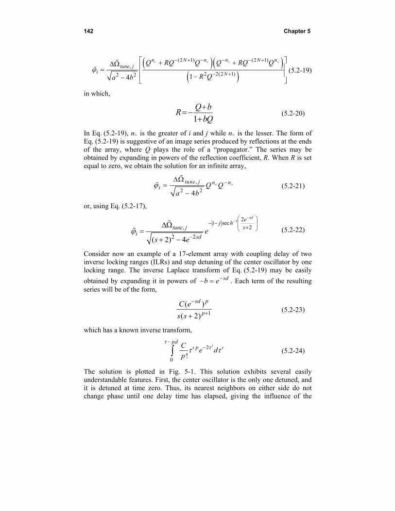
142 Chapter 5
(2 1) (2 1)
,
2 2(2 1)2 2 14
n n n nN Ntune j
i N
Q RQ Q Q RQ Q
R Qa b
(5.2-19)
in which,
1
Q bR
bQ
(5.2-20)
In Eq. (5.2-19), n> is the greater of i and j while n< is the lesser. The form of Eq. (5.2-19) is suggestive of an image series produced by reflections at the ends of the array, where Q plays the role of a “propagator.” The series may be obtained by expanding in powers of the reflection coefficient, R. When R is set equal to zero, we obtain the solution for an infinite array,
,
2 24
tune j n ni Q Q
a b
(5.2-21)
or, using Eq. (5.2-17),
1 2sec
2,
2 2( 2) 4
sdei j h
stune ji sd
es e
(5.2-22)
Consider now an example of a 17-element array with coupling delay of two inverse locking ranges (ILRs) and step detuning of the center oscillator by one locking range. The inverse Laplace transform of Eq. (5.2-19) may be easily
obtained by expanding it in powers of sdb e . Each term of the resulting series will be of the form,
1
( )
( 2)
sd p
p
C e
s s
(5.2-23)
which has a known inverse transform,
2
0!
pdpCe d
p
(5.2-24)
The solution is plotted in Fig. 5-1. This solution exhibits several easily understandable features. First, the center oscillator is the only one detuned, and it is detuned at time zero. Thus, its nearest neighbors on either side do not change phase until one delay time has elapsed, giving the influence of the
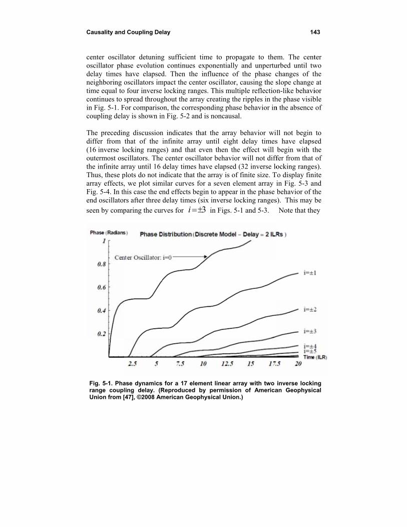
Causality and
center oscilloscillator phdelay times neighboring time equal tocontinues to in Fig. 5-1. Fcoupling dela The precedindiffer from (16 inverse loutermost osthe infinite arThus, these parray effects,Fig. 5-4. In thend oscillator
seen by comp
Fig. 5-1. Pharange couplUnion from [
d Coupling De
ator detuningase evolutionhave elapsedoscillators im
o four inverse spread throug
For comparisoay is shown in
ng discussionthat of the ocking rangecillators. Therray until 16
plots do not in, we plot simhis case the ers after three
paring the cur
ase dynamicsling delay. (R[47], ©2008 Am
lay
g sufficient tn continues ed. Then the
mpact the centlocking rang
ghout the arraon, the correspn Fig. 5-2 and
n indicates thinfinite array
es) and that ee center oscilldelay times h
ndicate that thmilar curves fo
nd effects begdelay times (
rves for i
for a 17 elemReproduced bmerican Geop
time to propexponentially influence of
ter oscillator, ges. This multay creating theponding phasd is noncausal
hat the array y until eight even then thelator behaviorhave elapsed he array is of or a seven elegin to appear six inverse lo3 in Figs. 5-
ment linear arby permissionhysical Union
pagate to theand unpertu
f the phase ccausing the s
tiple reflectioe ripples in thse behavior inl.
behavior widelay times
e effect will r will not diff(32 inverse lo
f finite size. Tement array iin the phase
ocking ranges
-1 and 5-3.
rray with two n of America
n.)
14
em. The centurbed until twchanges of thslope change n-like behavi
he phase visibn the absence
ll not begin s have elapsbegin with thfer from that ocking range
To display finiin Fig. 5-3 anbehavior of th
s). This may b
Note that the
inverse lockinan Geophysic
43
ter wo the at
ior ble of
to ed
the of s). ite nd the be
ey
ng cal
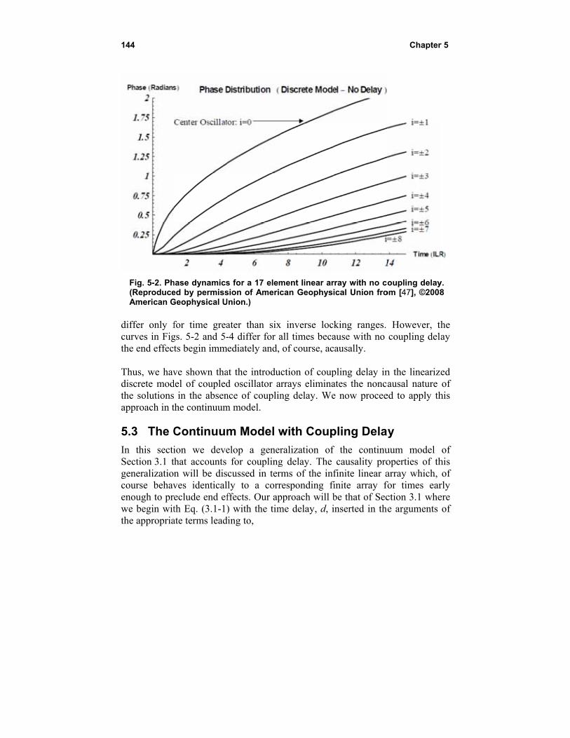
144
Fig. 5-2. Ph(ReproduceAmerican G
differ only fcurves in Figthe end effec Thus, we havdiscrete modthe solutionsapproach in t
5.3 The C
In this sectiSection 3.1 tgeneralizatiocourse behavenough to prwe begin witthe appropria
hase dynamicsed by permissGeophysical U
for time greags. 5-2 and 5-ts begin imm
ve shown thadel of coupled in the absenthe continuum
Continuum
ion we devethat accounts n will be disves identicaleclude end efth Eq. (3.1-1)ate terms lead
s for a 17 elemsion of Americ
Union.)
ater than six-4 differ for a
mediately and,
at the introdud oscillator ance of couplinm model.
m Model w
elop a generfor coupling
cussed in terly to a corrffects. Our ap) with the tim
ding to,
ment linear arcan Geophysi
x inverse locall times becaof course, ac
uction of couparrays eliminang delay. We
with Coup
ralization of g delay. The rms of the infresponding fipproach will bme delay, d, i
rray with no cical Union fro
king ranges. ause with no causally.
pling delay inates the nonce now procee
pling Dela
f the continucausality pro
finite linear afinite array fbe that of Secinserted in th
Chapter
oupling delayom [47], ©2008
However, thcoupling del
n the linearizausal nature
ed to apply th
ay
uum model operties of tharray which, for times earction 3.1 whe
he arguments
r 5
y. 8
the ay
ed of
his
of his of
rly ere of
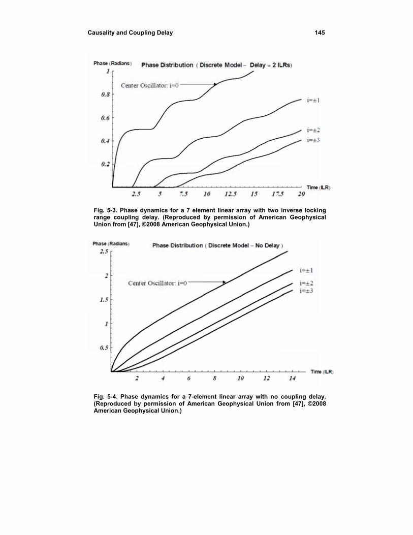
Causality and
Fig. 5-3. Phrange coupUnion from
Fig. 5-4. Ph(ReproduceAmerican G
d Coupling De
hase dynamicpling delay. ( [47], ©2008 A
hase dynamiced by permissGeophysical U
lay
s for a 7 elemReproduced
American Geo
cs for a 7-elemsion of Ameri
Union.)
ment linear arby permissiophysical Unio
ment linear aican Geophys
rray with two on of Americaon.)
rray with no sical Union fr
14
inverse lockinan Geophysic
coupling delarom [47], ©20
45
ng cal
ay. 08
146 Chapter 5
0
( , )( )
( , ) 2 ( , ) ( , )
ref
lock
d x tx
dtx x t d x t x x t d
(5.3-1)
Introducing the scaled time, τ, and the detuning function, ΔΩtune, as before, Laplace transformation leads to,
( , )
( , ) 2 ( , ) ( , )
tune
sd sd
s x s
x x s e x t x x s e
(5.3-2)
Then, expanding in Taylor series to second order in x ,
2
2
( , )2 2 ( , ) ( , )sd sd
tuned x s
s e x s x s edx
(5.3-3)
the analog of Eq. (3.1-4). Setting,
1
( , ) ( )tune x s x ys (5.3-4)
corresponding to step detuning of the oscillator at x = y at time zero by one locking range, we obtain the Green’s function, 1
~g , as the differential equation solution,
( 2) 2
1( , , )2 ( 2) 2
sdx y s esd
sd
eg s x y e
s s e
(5.3-5)
At this point, a serious difficulty is encountered with respect to causality. If one were to compute numerically the inverse Laplace transform integral for Eq. (5.3-5), one would find that the influence of the nearest neighbors of the detuned oscillator begins at time d. This violates causality because, as pointed out in Section 5.2, this influence must not begin until time 2d, the round trip transit time between the detuned oscillator and its neighbors. Following Pogorzelski [48], we begin our study of this apparent paradox by comparing the denominator of Eq. (5.3-5) with that of Eq. (5.2-22) known to be causal. That is, the denominator of Eq. (5.2-22) is,
2 2( 2) 4 ( 2) 2 ( 2) 2sd sd sds e s e s e (5.3-6)
while the denominator of Eq. (5.3-5) is,
Causality and Coupling Delay 147
( 2) 2 sds e (5.3-7)
Thus, the two solutions, the causal one Eq. (5.2-22), and the present one, Eq. (5.3-5), have different branch points in the complex s plane. Solution
Eq. (5.3-5) has branch points where 2 2 sds e whereas the causal solution
Eq. (5.2-22) has these plus additional branch points where 2 2 sds e . Now, computing the inverse Laplace transform via integration on the Bromwich contour will involve deformation of the contour around the branch cuts associated with these branch points. Thus, it becomes clear that the solution Eq. (5.3-5) will be missing the contribution from half of the branch cuts in the causal solution Eq. (5.2-22). As shown in [48], this is the root of the causality difficulty. Why do we find ourselves in this situation? Our approach was successful in the absence of coupling delay, but something went wrong when delay was included. This can be understood by looking at the nature of the solutions corresponding to the two sets of branch cuts shown in Fig. 5-5 where the dots correspond to Eq. (5.3-7) and the circles to the remaining branch points of the complete set, Eq. (5.3-6). We have assumed in deriving the partial differential equation Eq. (5.3-3) that the solution will be smoothly varying in the interior of the array so that the inter-oscillator phase differences are small validating the linearization of the sine functions in Adler’s formalism. Thus, in the interior of the array where the detuning is zero, the second derivative will be small and
2 2sds e (5.3-8)
corresponding to the dot branch points in Fig. 5-5. However, we can switch
from the dots to the circles by replacing sde with sde . Doing this in Eq. (5.3-2) we obtain,
1
1 1 1
( , )
( , ) 2 ( , ) ( , )
tune
sd
s x s
x x s e x t x x s
(5.3-9)
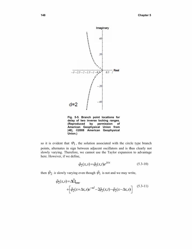
148
so it is evid
points, alternslowly varyinhere. Howeve
then 2 is sl
2
Fig. 5-delay o(ReproAmeric[48], ©Union.)
ent that 1 ,
nates in sign ng. Thereforeer, if we defin
lowly varying
2
2
( , )
(
tux s
x
-5. Branch pof two invers
oduced by can Geophys©2008 Amer)
the solution
between adje, we cannotne,
2( , )x s
g even though
, )
une
sdx x s e
point locationse locking ra
permissionsical Unionican Geophy
n associated w
acent oscillatt use the Tay
1( , ) j xx t e
h 1 is not an
22 ( , )x t
s for nges. of from
ysical
with the circ
tors and is thylor expansion
nd we may w
2( , )x x s
Chapter
cle type bran
hus clearly nn to advanta
(5.3-10)
write,
)(5.3-11)
r 5
nch
not age
Causality and Coupling Delay 149
and expand in Taylor series to obtain,
2
222
( , )2 2 ( , ) ( , )sd sd
tuned x s
s e x s x s edx
(5.3-12)
corresponding to the circle type branch points. Thus, it becomes clear that our assumption of slowly varying phase, implicit in the use of the Taylor series, eliminated the solutions associated with the circle type branch points. The Green’s function corresponding to these branch points is,
( 2) 2
( )2( , , )
2 ( 2) 2
sdj x y s esd j x y
sd
eg s x y e
sj s e
(5.3-13)
and the causal Green’s function is a linear combination of Eq. (5.3-5) and Eq. (5.3-13); that is,
2 ( 2) 2 ( 2)
( )( , , )2 2 ( 2) 2 2 ( 2)
sd sdj x y s e j x y s esd sd j x y
sd sd
e eg s x y A e B e
sj s e sj s e
(5.3-14)
where A + B = 1 so that the proper detuning function is generated on the right side of the differential equation. It remains to determine A and B. For large values of s, far from the origin of the s plane, we can obtain a fairly accurate estimate of the branch point locations. These locations are defined by,
2 2 sds e (5.3-15)
where the upper sign corresponds to the dots and the lower one to the circles. Inserting s j ,
2 2 d j dj e e
(5.3-16)
For 2 ,
/22 j dde e (5.3-17)
Thus,
150 Chapter 5
22pd p (5.3-18)
and we have
1
22n n
d
(5.3-19)
for the dots and
1
22m m
d
(5.3-20)
for the circles. Now, from Eq. (5.3-17),
0
2 dp e (5.3-21)
so,
1
ln2
pp d
(5.3-22)
for p = m or n. Armed with these approximate branch point locations, we are in a position to estimate ( , , ) /g y y , the time derivative of the phase of the detuned oscillator. This will exhibit the temporal discontinuities associated with the arrival of influence from neighboring oscillators and highlight the causal behavior. First, from Eq. (5.3-14),
( , , )2 2 ( 2) 2 2 ( 2)
sd sd
sd sd
e esg s y y A B
j s e j s e
(5.3-23)
Now, envisioning the inverse transform as a sum of branch cut integrals, we recognize that the result will be approximately,
Causality and Coupling Delay 151
1 /1
1 /0
2sin
( , , ) 122 1
22 1
2sin
122 1
2
dnn d
dmm d
ng y y d d
A Add
md d
Bd
(5.3-24)
Here we have used the s’s given by Eq. (5.3-19) through Eq. (5.3-22) and,
( )
0
u dedu
du
(5.3-25)
The expression on the right side of Eq. (5.3-24) is a Fourier series except for the time dependence of the coefficients. Recall that this series was obtained using the large s approximation so only the high-order terms are accurate. The high-order terms of this series govern the discontinuities in the time
dependence. Now, looking at Eq. (5.3-24) for d ,
21
20
1sin 2
2( , , ) 12 1
22 1
1sin 2
2 12 1
2
nn d
mm d
ng y y
A Add
m
Bd
(5.3-26)
and we see that if A = B, the high-order portions of the two series will cancel
term by term so that there will be no discontinuity at d . However, at
2d we have,
152 Chapter 5
31
30
sin 4 1( , , ) 12 1
22 1
sin 4 1 12 1
2
nn d
mm d
ng y yA A
dd
mB
d
(5.3-27)
and the high-order terms no longer cancel but add. Thus, there will be a
discontinuity at 2d . This is to be expected because it allows for one round-trip interval to the nearest neighbors from the time when the oscillator is detuned. We conclude that the discontinuities will occur at the proper times for causality to be satisfied only if A = B. From this condition and the fact that A + B = 1, we determine that both A and B are equal to ½, and from Eq. (5.3-14) the causal Green’s function is,
2 ( 2) 2 ( 2)
( )( , , )4 2 ( 2) 4 2 ( 2)
sd sdj x y s e j x y s esd sd j x y
sd sd
e eg s x y e e
sj s e sj s e
(5.3-28)
As shown in Ref. [48], a better approximation to the exact discrete model solution may be obtained from the form,
2 ( 2) 2 ( 2)
( )( , , )4 2 ( 2) 4 2 ( 2)
sd sdj x yC s e j x yC s esd sd j x y
sd sd
e eg s x y C e C e
sj s e sj s e
(5.3-29)
with optimal selection of the constant, C. From Ref. [48], the optimal value of C is,
2 2
C
(5.3-30)
The temporal behavior of the phase of each oscillator in the array is most easily seen by plotting the time derivative of the phase because this makes more obvious the times at which the influences from the neighboring oscillators arrive. Thus, in Figs. 5-6 through 5-10, we compare the result of the approximate continuum formula Eq. (5.3-29) in solid lines with that of the discrete model Eq. (5.2-22) in dashed lines considered to be the exact result. The coupling delay in this example is two inverse locking ranges (ILRs). The fine scale wiggles shown in the inset of Fig. 5-6 arise from the truncation of the series of branch cut integrals to a finite number of terms.
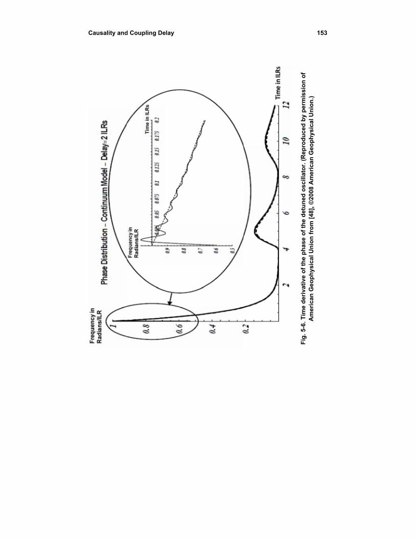
Causality and
d Coupling Delay
15
Fig
. 5-6
. Tim
e d
eriv
ativ
e o
f th
e p
has
e o
f th
e d
etu
ned
osc
illat
or.
(R
epro
du
ced
by
per
mis
sio
n o
f A
mer
ican
Geo
ph
ysic
al U
nio
n f
rom
[48
], ©
200
8 A
me
rica
n G
eop
hys
ica
l Un
ion
.)
53
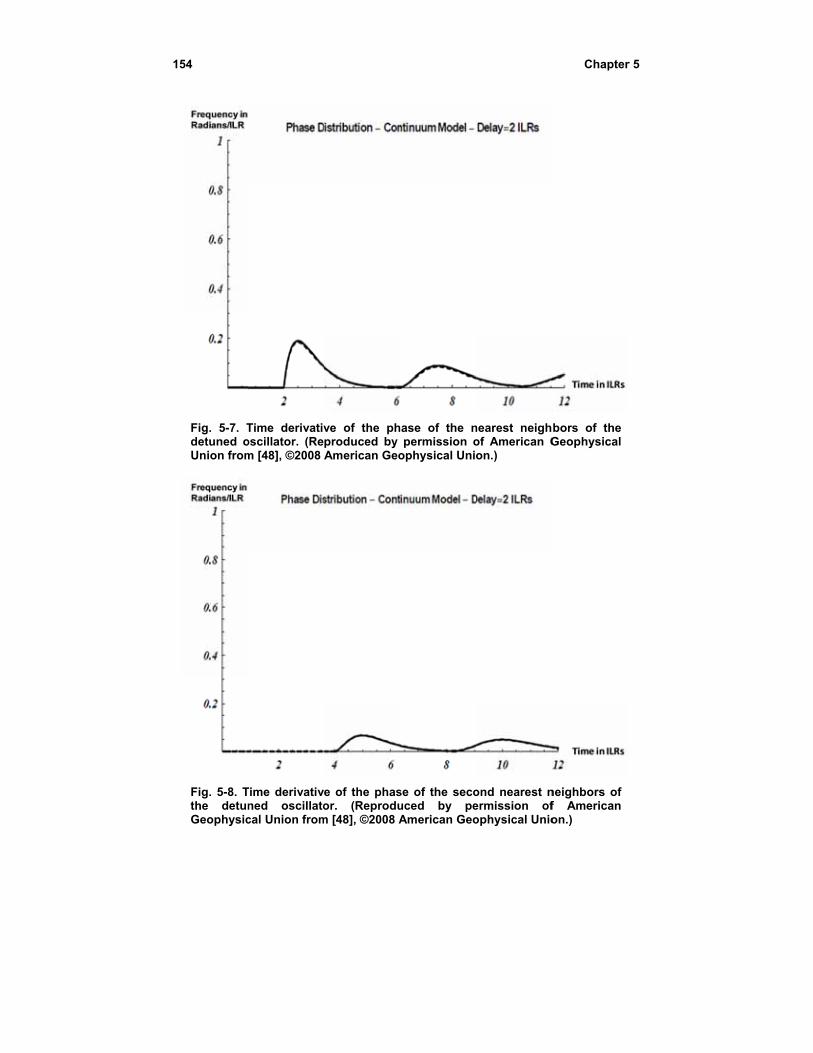
154
Fig. 5-7. Tdetuned oUnion from
Fig. 5-8. Tthe detunGeophysic
Time derivativoscillator. (Rem [48], ©2008
Time derivativned oscillatocal Union from
ve of the phproduced by American Geo
e of the phasor. (Reprodu
m [48], ©2008 A
hase of the npermission o
ophysical Uni
se of the secouced by peAmerican Geo
nearest neighof American Gon.)
ond nearest nermission ofophysical Unio
Chapter
bors of the Geophysical
neighbors of f American on.)
r 5

Causality and
Fig. 5-9.the detGeophys
Fig. 5-1of the Geophy
d Coupling De
. Time derivattuned oscillasical Union fro
10. Time derivdetuned osc
ysical Union f
lay
tive of the phator. (Reprodom [48], ©200
vative of the pillator. (Repro
from [48], ©20
ase of the thiduced by pe
8 American G
hase of the fooduced by pe08 American G
ird nearest neermission of Geophysical U
ourth nearest nermission of Geophysical U
15
eighbors of
American nion.)
neighbors American
Union.)
55
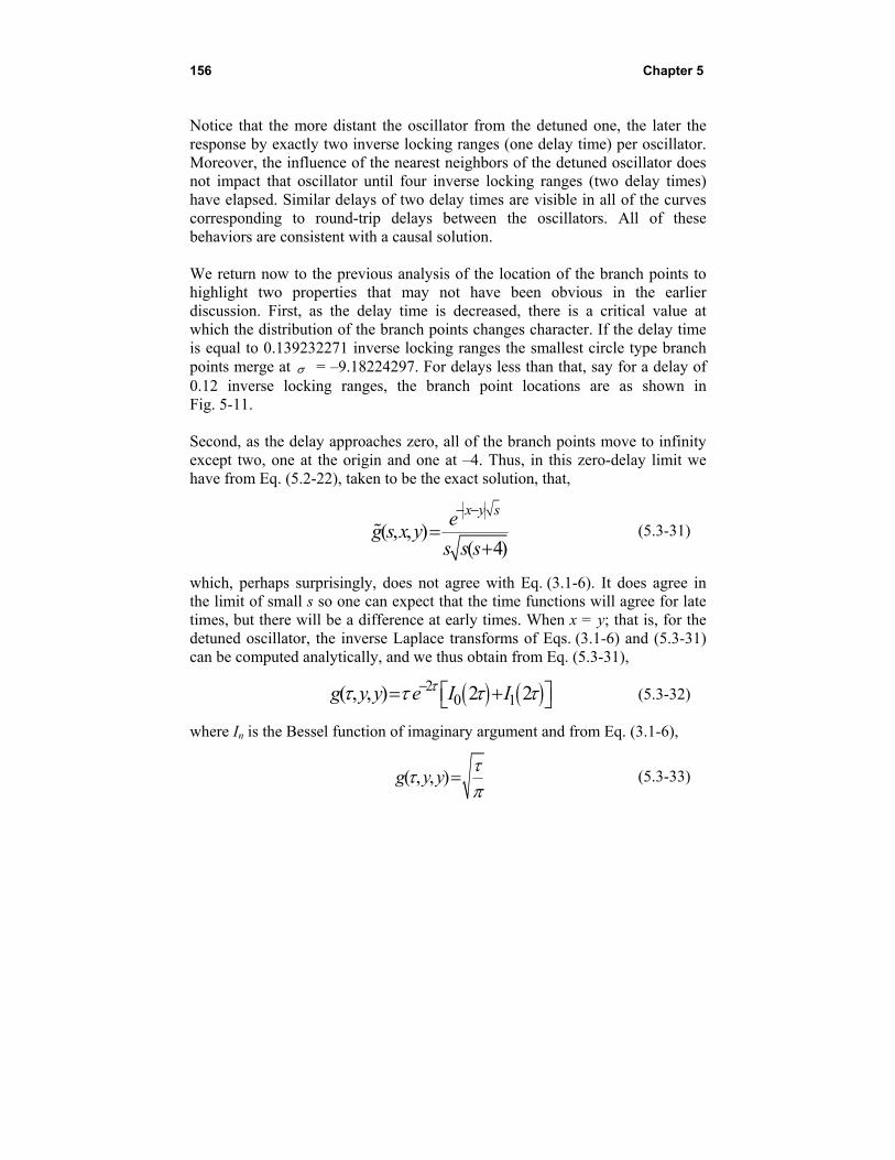
156 Chapter 5
Notice that the more distant the oscillator from the detuned one, the later the response by exactly two inverse locking ranges (one delay time) per oscillator. Moreover, the influence of the nearest neighbors of the detuned oscillator does not impact that oscillator until four inverse locking ranges (two delay times) have elapsed. Similar delays of two delay times are visible in all of the curves corresponding to round-trip delays between the oscillators. All of these behaviors are consistent with a causal solution. We return now to the previous analysis of the location of the branch points to highlight two properties that may not have been obvious in the earlier discussion. First, as the delay time is decreased, there is a critical value at which the distribution of the branch points changes character. If the delay time is equal to 0.139232271 inverse locking ranges the smallest circle type branch points merge at = –9.18224297. For delays less than that, say for a delay of 0.12 inverse locking ranges, the branch point locations are as shown in Fig. 5-11. Second, as the delay approaches zero, all of the branch points move to infinity except two, one at the origin and one at –4. Thus, in this zero-delay limit we have from Eq. (5.2-22), taken to be the exact solution, that,
( , , )( 4)
x y seg s x y
s s s
(5.3-31)
which, perhaps surprisingly, does not agree with Eq. (3.1-6). It does agree in the limit of small s so one can expect that the time functions will agree for late times, but there will be a difference at early times. When x = y; that is, for the detuned oscillator, the inverse Laplace transforms of Eqs. (3.1-6) and (5.3-31) can be computed analytically, and we thus obtain from Eq. (5.3-31),
20 1( , , ) 2 2g y y e I I (5.3-32)
where In is the Bessel function of imaginary argument and from Eq. (3.1-6),
( , , )g y y
(5.3-33)
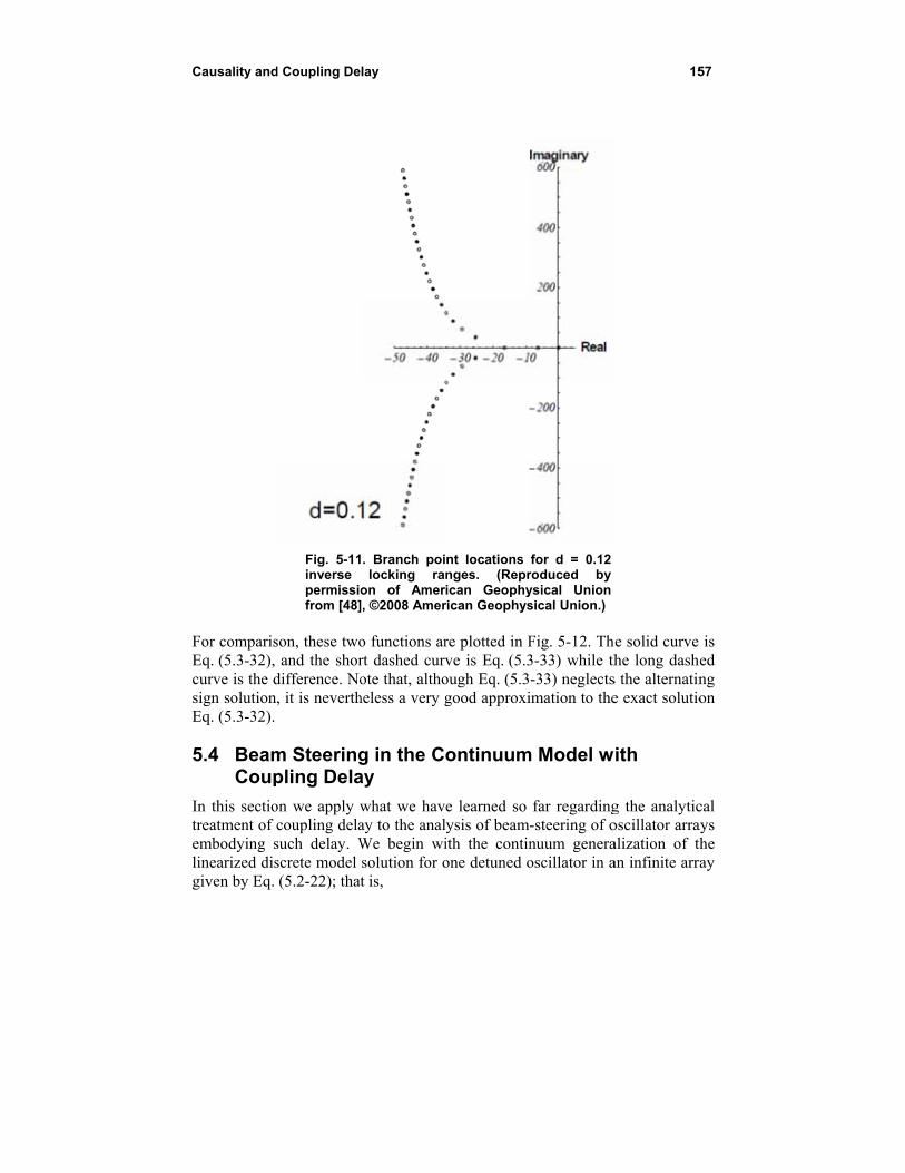
Causality and
For comparisEq. (5.3-32), curve is the dsign solutionEq. (5.3-32).
5.4 BeamCoup
In this sectiotreatment of embodying slinearized disgiven by Eq.
d Coupling De
Fig. 5-11inverse permissiofrom [48]
son, these twoand the shor
difference. Non, it is neverth
m Steeringpling Dela
on we apply wcoupling delasuch delay. Wscrete model (5.2-22); that
lay
. Branch poilocking ra
on of Amer], ©2008 Amer
o functions arrt dashed curvote that, altho
heless a very g
g in the Cay
what we havay to the analWe begin wisolution for ot is,
nt locations nges. (Repr
rican Geophyrican Geophys
re plotted in Fve is Eq. (5.3ough Eq. (5.3good approxi
ontinuum
e learned so lysis of beam-ith the continone detuned o
for d = 0.12 roduced by ysical Unionsical Union.)
Fig. 5-12. Th3-33) while th-33) neglectsimation to the
m Model w
far regarding-steering of onuum generaoscillator in a
15
he solid curve he long dash
s the alternatine exact solutio
ith
g the analyticoscillator arraalization of tan infinite arr
57
is hed ng on
cal ays the ray
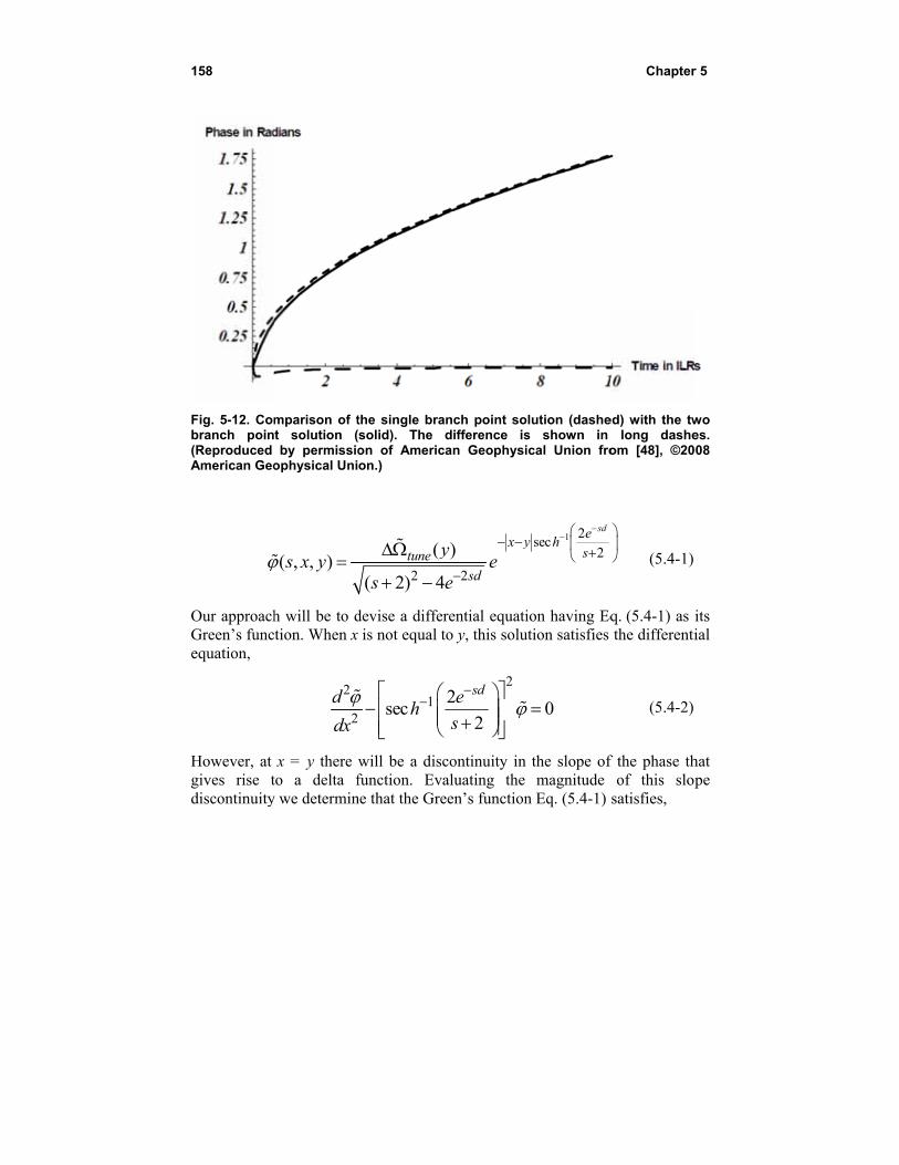
158
Fig. 5-12. Combranch poin(Reproduced American Geo
Our approachGreen’s funcequation,
However, at gives rise tdiscontinuity
mparison of tt solution (by permissio
ophysical Uni
( , , )s x y
h will be to dction. When x
2
2
d
dx
x = y there to a delta fy we determin
the single brasolid). The on of Americon.)
2
(
( 2) 4
tune y
s
devise a diffeis not equal t
1sech
will be a disfunction. Evne that the Gre
anch point sodifference is
can Geophysi
2
)
4
x y
sd
ye
e
erential equatito y, this solu
22
2
sde
s
continuity in aluating the een’s function
olution (dashes shown in ical Union fro
1 2sec
2
sdey h
s
ion having Eqution satisfies
0
the slope ofmagnitude
n Eq. (5.4-1)
Chapter
ed) with the twlong dashe
om [48], ©20
(5.4-1)
q. (5.4-1) as the differenti
(5.4-2)
f the phase thof this slop
satisfies,
r 5
wo es.
008
its ial
hat pe
Causality and Coupling Delay 159
22
12
1
2 2
2sec
2
22sec
2( ) ( )
( 2) 4
sd
sd
tune sd
d eh
sdx
eh
sy x y
s e
(5.4-3)
We may now follow the procedure of Section 3.1 to express the finite-array Green’s function as a sum of the eigenfunctions of the differential operator in this equation. In order to do this we will need the boundary conditions at the ends of the array. Recall that the reflection coefficient at the array ends was given by Eq. (5.2-20) which is a fairly complicated function of s. However, following Pogorzelski [49], we may simplify matters by assuming the addition of half-length coupling lines at the ends of the array. If this is done, the reflection coefficient becomes unity because the array boundary then becomes an image plane. (See Pogorzelski [47].) A reflection coefficient of unity corresponds to the familiar Neumann condition of zero phase slope. Using this boundary condition, the even and odd normalized eigenfunctions are seen to be,
2 2cos
2 12 1
2 12sin
2 12 1
ne
no
n x
NN
n x
NN
(5.4-4)
Choosing the detuning time dependence to be a unit step at time zero and following he approach of Section 3.1, the Laplace transform of the phase distribution may be written in terms of the eigenfunctions as,
160 Chapter 5
1
2 2
221
2
24sec
2( , , )
(2 1) ( 2) 4
2 2cos cos
2 1 2 1
2 2sec
2 1 2
2 1 2 1sin sin
2 1 2 1
2 1
2 1
sd
sd
sdn
eh
ss x y
N s s e
n y n xN N
n eh
N s
n y n x
N N
n
N
2
1 2sec
2
sdeh
s
(5.4-5)
We will obtain the inverse Laplace transform via residue calculus. The poles are determined by,
1 2sec
2 1
sde ih
s N
(5.4-6)
Taking the hyperbolic secant of both sides and then the reciprocal we obtain the equivalent condition,
2
cos2 12 sd
s
Ne
(5.4-7)
This equation can be solved in terms of the Lambert W function defined by,
( )( ) W zz W z e (5.4-8)
In terms of this function, the solution of Eq. (5.4-7) is,
1
, 2 cos 22 1
sdms W m de
d N
(5.4-9)
These pole locations are plotted in Fig. 5-13.
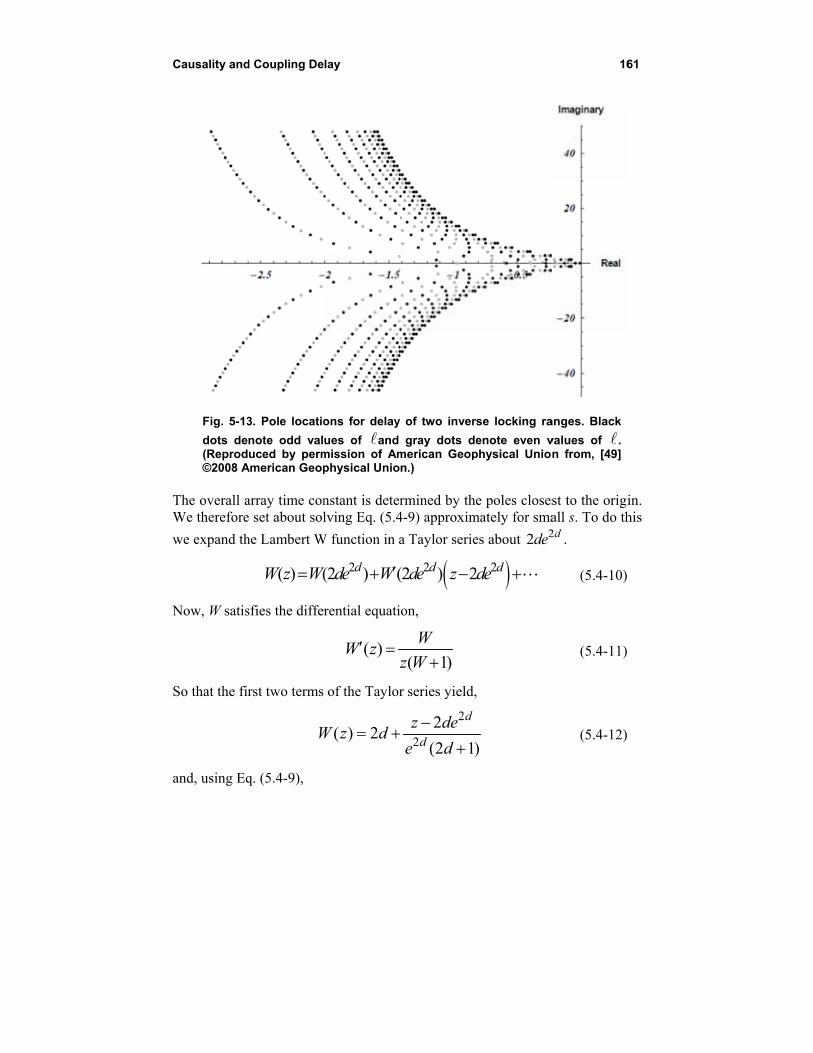
Causality and
Fig. 5-13
dots de(Reprod©2008 A
The overall aWe therefore
we expand th
Now, W satis
So that the fi
and, using Eq
d Coupling De
3. Pole locatio
note odd valuced by perm
American Geop
array time cone set about sol
he Lambert W
( ) (W z W
sfies the diffe
rst two terms
W
q. (5.4-9),
lay
ons for delay
ues of and mission of Amphysical Unio
nstant is deterlving Eq. (5.4
W function in a
2(2 ) (dW de W
rential equati
( )W zz
of the Taylor
( ) 2W z d
y of two inver
gray dots demerican Geopn.)
rmined by the4-9) approxim
a Taylor serie
2(2 ) 2dde z
ion,
( 1)
W
z W
r series yield,
2
2
2
(2 1)
d
d
z de
e d
rse locking ra
enote even vphysical Union
e poles closesmately for sma
es about 22de
22 dde
,
)
16
anges. Black
values of . n from, [49]
st to the origiall s. To do th2d .
(5.4-10)
(5.4-11)
(5.4-12)
61
in. his
162 Chapter 5
2
2
2
(2 1)
d
m d
z des
e d
(5.4-13)
Recall that z is the argument of the W function so from Eq. (5.4-9),
2 cos2 1
sdz deN
(5.4-14)
Substituting Eq. (5.4-14) into Eq. (5.4-13) and setting m = 0,
2
20 2
2 cos 242 1
sin2 1 2 1(2 1)
sd d
d
de deN
sd Ne d
(5.4-15)
The pole at 0 together with the denominator s from the step detuning function produce the double pole at the origin leading to the linear time dependence or shift in ensemble frequency due to the detuning. For the antisymmetric detuning used in beam-steering, the even poles do not contribute, so the dominant pole is the one for 1 lying on the real axis at,
2
201
4 / 2 1sin
2 1 2 1 2 1 2 1s
d N d N
(5.4-16)
so the time constant of the array is,
2
2 12 1c
Nd
(5.4-17)
or just (2d+1) times the time constant without coupling delay. (Compare with Eq. (2.2-40).) Returning now to Eq. (5.4-5), we form the solution for beam-steering by combining two solutions of the form Eq. (5.4-5), one for detuning of the oscillator at –N and one for detuning of the oscillator at N, each end of the array.
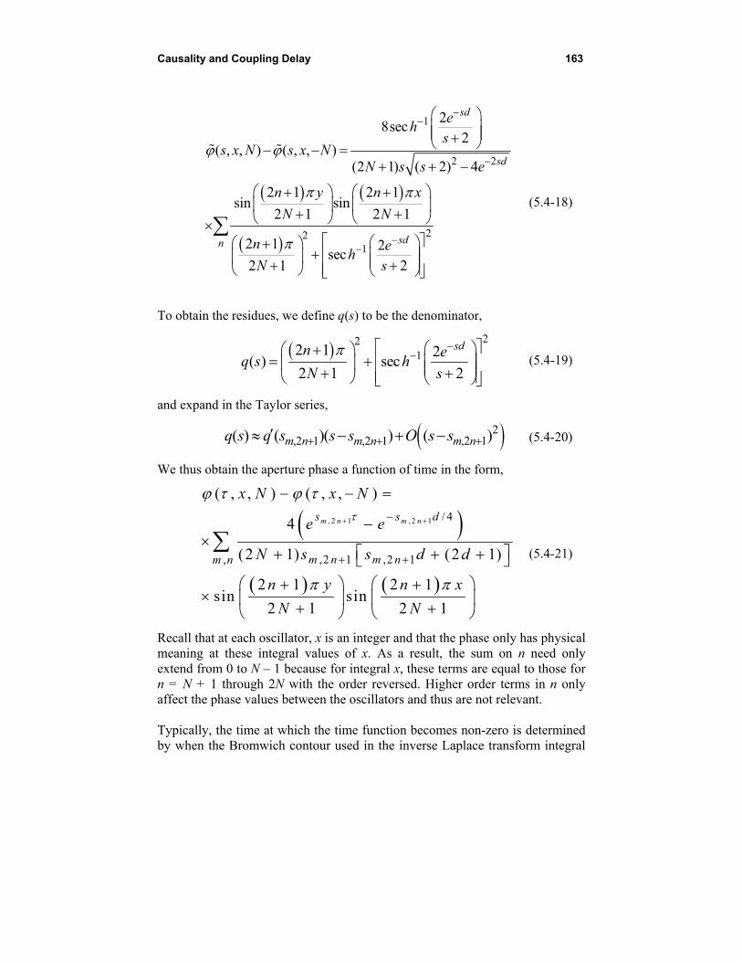
Causality and Coupling Delay 163
1
2 2
221
28sec
2( , , ) ( , , )
(2 1) ( 2) 4
2 1 2 1sin sin
2 1 2 1
2 1 2sec
2 1 2
sd
sd
sdn
eh
ss x N s x N
N s s e
n y n x
N N
n eh
N s
(5.4-18)
To obtain the residues, we define q(s) to be the denominator,
2212 1 2
( ) sec2 1 2
sdn eq s h
N s
(5.4-19)
and expand in the Taylor series,
2,2 1 ,2 1 ,2 1( ) ( )( ) ( )m n m n m nq s q s s s O s s (5.4-20)
We thus obtain the aperture phase a function of time in the form,
, 2 1 , 2 1 / 4
,2 1 ,2 1,
( , , ) ( , , )
4
(2 1) (2 1)
2 1 2 1sin sin
2 1 2 1
m n m ns s d
m n m nm n
x N x N
e e
N s s d d
n y n x
N N
(5.4-21)
Recall that at each oscillator, x is an integer and that the phase only has physical meaning at these integral values of x. As a result, the sum on n need only extend from 0 to N – 1 because for integral x, these terms are equal to those for n = N + 1 through 2N with the order reversed. Higher order terms in n only affect the phase values between the oscillators and thus are not relevant. Typically, the time at which the time function becomes non-zero is determined by when the Bromwich contour used in the inverse Laplace transform integral
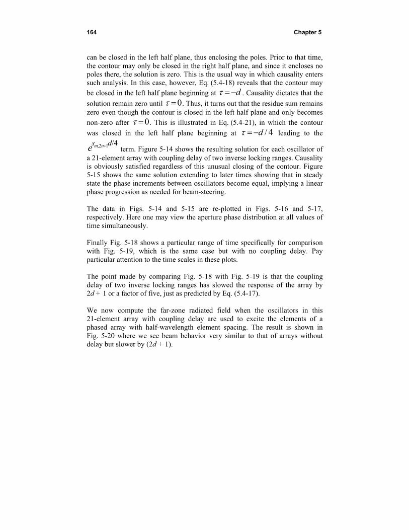
164 Chapter 5
can be closed in the left half plane, thus enclosing the poles. Prior to that time, the contour may only be closed in the right half plane, and since it encloses no poles there, the solution is zero. This is the usual way in which causality enters such analysis. In this case, however, Eq. (5.4-18) reveals that the contour may
be closed in the left half plane beginning at d . Causality dictates that the
solution remain zero until 0 . Thus, it turns out that the residue sum remains zero even though the contour is closed in the left half plane and only becomes
non-zero after 0 . This is illustrated in Eq. (5.4-21), in which the contour
was closed in the left half plane beginning at / 4d leading to the
,2 1 /4m ns de term. Figure 5-14 shows the resulting solution for each oscillator of a 21-element array with coupling delay of two inverse locking ranges. Causality is obviously satisfied regardless of this unusual closing of the contour. Figure 5-15 shows the same solution extending to later times showing that in steady state the phase increments between oscillators become equal, implying a linear phase progression as needed for beam-steering. The data in Figs. 5-14 and 5-15 are re-plotted in Figs. 5-16 and 5-17, respectively. Here one may view the aperture phase distribution at all values of time simultaneously. Finally Fig. 5-18 shows a particular range of time specifically for comparison with Fig. 5-19, which is the same case but with no coupling delay. Pay particular attention to the time scales in these plots. The point made by comparing Fig. 5-18 with Fig. 5-19 is that the coupling delay of two inverse locking ranges has slowed the response of the array by 2d + 1 or a factor of five, just as predicted by Eq. (5.4-17). We now compute the far-zone radiated field when the oscillators in this 21-element array with coupling delay are used to excite the elements of a phased array with half-wavelength element spacing. The result is shown in Fig. 5-20 where we see beam behavior very similar to that of arrays without delay but slower by (2d + 1).
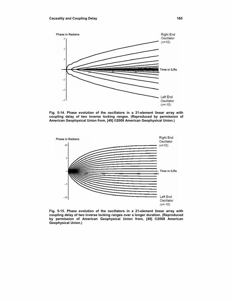
Causality and
Fig. 5-14. Phcoupling delaAmerican Geo
Fig. 5-15. Phcoupling delaby permissioGeophysical
d Coupling De
hase evolutionay of two invophysical Uni
hase evolutionay of two inveon of AmericUnion.)
lay
n of the osciverse lockingon from, [49] ©
n of the oscirse locking racan Geophys
illators in a 2g ranges. (Re©2008 Americ
illators in a 2anges over a lsical Union f
21-element lineproduced bycan Geophysic
21-element linonger duratiofrom, [49] ©2
16
near array wiy permission cal Union.)
near array wion. (Reproduc2008 Americ
65
ith of
ith ed an
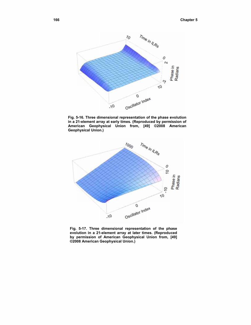
166
Fig. 5in a 2AmerGeop
Fig. evolby p©20
5-16. Three di21-element arrrican Geophphysical Union
5-17. Three lution in a 21permission o08 American G
mensional repray at early tim
hysical Union.)
dimensional -element arra
of American GGeophysical U
presentation omes. (Reprodun from, [49
representatioay at later timGeophysical UUnion.)
of the phase euced by perm9] ©2008 A
on of the phmes. (Reprodu
Union from,
Chapter
evolution mission of American
hase ced [49]
r 5
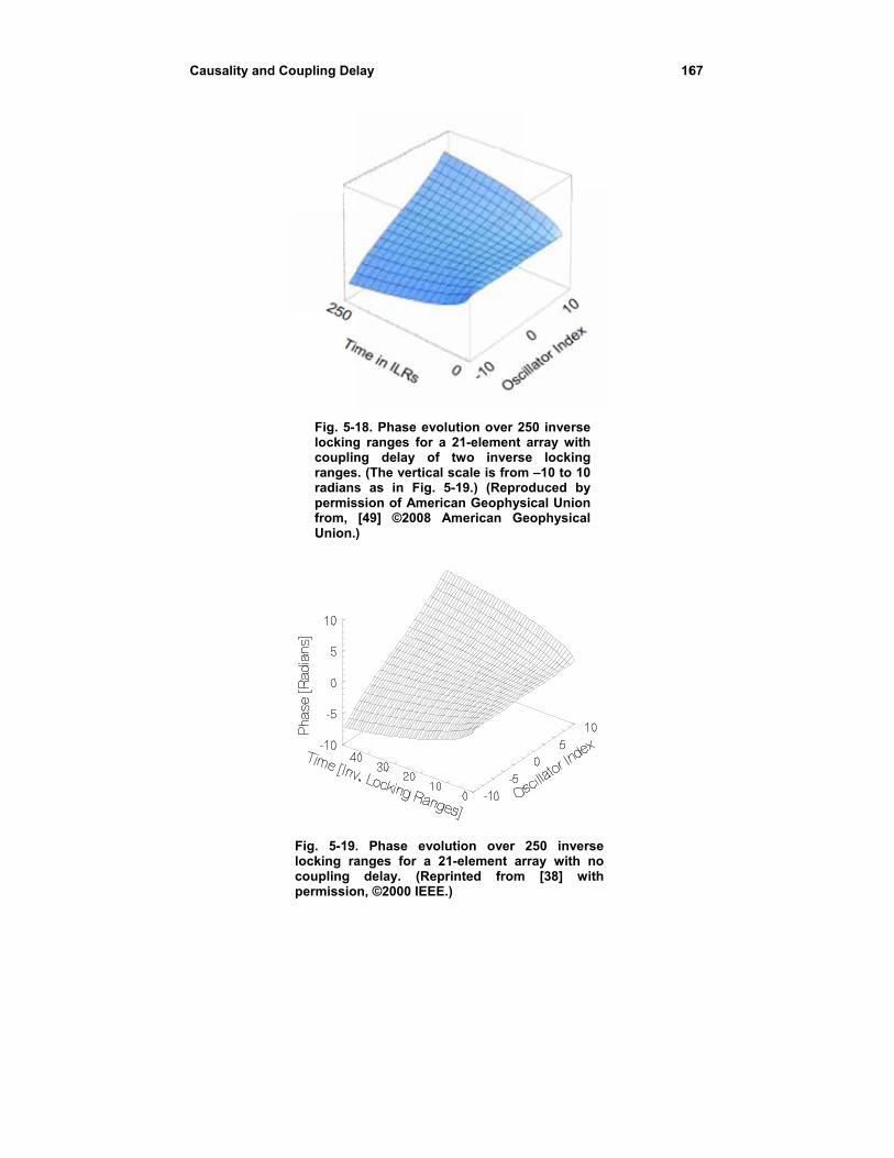
Causality and
d Coupling De
Fig. 5-1lockingcouplinrangesradianspermisfrom, Union.)
Fig. 5-19.locking racoupling permissio
lay
18. Phase evog ranges for ang delay of s. (The verticas as in Fig.
ssion of Amer[49] ©2008 )
. Phase evoanges for a 2
delay. (Repon, ©2000 IEEE
olution over 2a 21-element f two inversl scale is from5-19.) (Repro
rican GeophysAmerican Ge
olution over 21-element arprinted fromE.)
250 inverse array with
se locking m –10 to 10 oduced by sical Union eophysical
250 inverse rray with no
m [38] with
1667
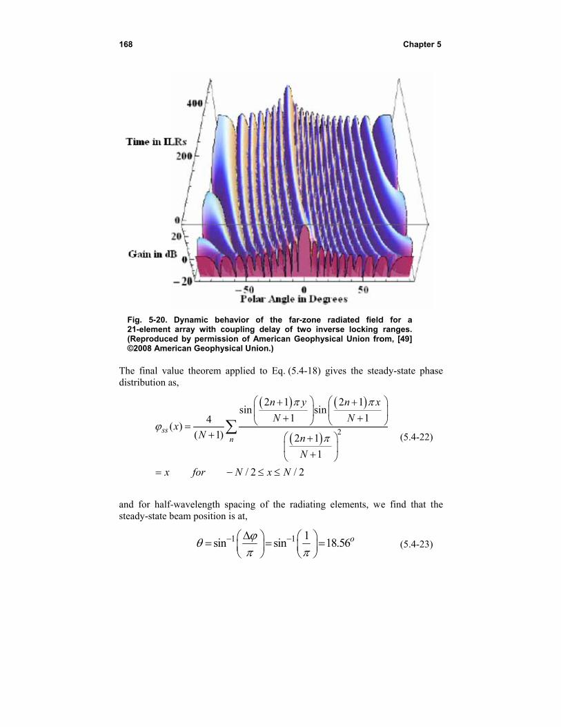
168
Fig. 5-20. 21-element (Reproduce©2008 Ame
The final vadistribution a
(ss
x
and for half-steady-state b
Dynamic bearray with c
ed by permisserican Geophy
alue theorem as,
4( )
( 1)x
N
for
f-wavelength beam position
sin
ehavior of thcoupling delaysion of Ameriysical Union.)
applied to E
2sin
/ 2
n
n
N
N x
spacing of thn is at,
1n s
he far-zone ry of two invecan Geophys
Eq. (5.4-18) g
1sin
1
2 1
1
/ 2
y
N
n
N
N
he radiating
1 1sin 1
radiated fielderse locking
sical Union fro
gives the stea
2
2 1
1
n x
N
elements, we
18.56o
Chapter
d for a ranges.
om, [49]
ady-state pha
(5.4-22)
e find that th
(5.4-23)
r 5
ase
the
Causality and Coupling Delay 169
This one-radian inter-oscillator phase difference stresses the linear approximation a bit in that the error in linearizing the sine function is about 19 percent. However, the dynamic behavior is still qualitatively approximated. In the above analysis a large number of residues are required for early times and very few are required for late times. However, returning to the discrete model, an alternative formulation is available that provides for more efficient computation for early times. Returning to Eq. (5.2-19) and specializing to the present case of a 21-element array, we have that,
21 10 21 10
422 2
10 21 10 21
42
10
212 2
1( , )
14
1
1
14
x x
x x
x x
Q Q Q Q Q Qf s x
Qs a b
Q Q Q Q Q Q
Q
Q QQ Q
Qs a b
(5.4-24)
where as before, 0 1a s , 2a s , and sdb e . We now expand this
expression in powers of –b, and as before, the inverse Laplace transform of each term in the expansion can be computed analytically. The number of terms required is determined by the time interval over which the response is desired
because each term has a delay factor psde where p is the power of –b in the term in the expansion, and d is the coupling delay. So, for sufficiently large p, the term will be zero for the interval in question. Thus, in contrast with the eigenfunction expansion, for early times very few terms are required. This approach was applied to the 21-element array with coupling delay treated earlier, and the results are plotted in Fig. 5-21 for comparison with Fig. 5-14. Interestingly, this power series approach is a bit more flexible in terms of boundary conditions. Recall that without the added half-length coupling lines at each end of the array, the previous method was complicated. Here, however, the use of Eq. (5.2-20) in Eq. (5.2-19) to model an array without the added lines poses no difficulty. The expansion in powers of b proceeds as before and the result is plotted in Fig. 5-22. Notice the difference in the early time ripples due to this alternative boundary condition when compared with Fig. 5-21.
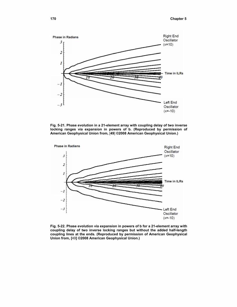
170
Fig. 5-21. Phalocking rangeAmerican Geo
Fig. 5-22. Phacoupling delacoupling linesUnion from, [4
ase evolution es via expanophysical Uni
ase evolution vay of two inves at the ends49] ©2008 Am
in a 21-elemennsion in poweon from, [49] ©
via expansionerse locking . (Reproduced
merican Geoph
nt array with cers of b. (Re©2008 Americ
n in powers of ranges but wd by permissihysical Union.
coupling delayeproduced bycan Geophysic
b for a 21-elewithout the ad
on of Americ)
Chapter
y of two invery permission cal Union.)
ement array widded half-lengan Geophysic
r 5
rse of
ith gth cal
Causality and Coupling Delay 171
5.5 Conclusion
The primary motivation for this chapter was the issue of causality in coupled oscillator arrays. Because the continuum model leads to a diffusion equation, the response to an excitation always begins immediately regardless of the physical separation of the two. Here, by appropriately introducing a delay factor in the Laplace transforms, we render the solutions causal in that there appears a finite “propagation delay” between the excitation and the response. The result is a more realistic representation of the array response not to mention some rather interesting inverse Laplace transforms encountered along the way.

172 Chapter 5
173
Part II: Experimental Work and Applications
Chapter 6 Experimental Validation of the Theory
Much of the very early work in coupled oscillators for phased-array applications involved both theory and experiment. Probably the earliest was the work of Karl Stephan in which he studied a linear array of coupled oscillators for beam-steering of a linear array of radiating elements [1]. In his concept, the phasing was controlled by injection locking the end oscillators to signals whose relative phase was controlled with a phase shifter. While still earlier work was published, Stephan points out that it did not involve mutual injection locking, the defining feature of the concepts treated in this book.
6.1 Linear-Array Experiments
Stephan’s pioneering experiment in 1986 involved three very high frequency (VHF) transistor Colpitts oscillators coupled together by a network of lumped elements. The end oscillators were also injected with external signals derived from a master oscillator signal that was split into two signals, one of which was phase shifted relative to the other by a variable length transmission line (coaxial line stretcher). Stephan measured the oscillator phases with varying amounts of phase shift of the injection signals and verified that the behavior conformed qualitatively to the theory. However, he noted several issues that have persisted throughout the ensuing development of this technology. He noted that manufacturing variation among the oscillators resulting in variation in their free-
174 Chapter 6
running frequencies causes nonuniformity in the array behavior and indicated an appreciation of the fact that in his VHF oscillators this can be compensated for with tuning, but that in a monolithic microwave integrated circuit (MMIC) such adjustment would be more difficult. He did some statistical studies of this issue, and such studies were more recently extended by Wang and Pearson [50]. Their approach to mitigating this problem was to design the oscillator to minimize the phase slope of the open-loop gain. The impact of free-running frequency variation on beam pointing was studied by Shen and Pearson [51]. In his early work Stephan also discussed high-frequency application in spatial power combining and beam-steering, pointing out that there is potential for graceful degradation in the event of oscillator failure. Interestingly, he used a gradual phase shift of the injection signals (as discussed in Section 3.4 above) rather than a step-phase shift in time. The next year, Stephan and Young published theoretical and experimental results concerning two mutually injection-locked oscillators where the coupling was provided by the free-space mutual coupling between the radiating elements excited by them. [3] The coupling was represented by a two-by-two admittance matrix, and the stability of the two modes, even and odd, for the system was treated. The radiation patterns as a function of coupling phase; that is, element separation, showed behavior consistent with the analysis. Three years later, Robert York, then a student working under Professor Richard Compton at Cornell University, published the results of a study of power combining in mutually injection locked Gunn diode oscillators arranged in a four-by-four planar array with Cartesian coupling [4]. Beam steering, however, was not considered; probably at least partly motivated by the publication by James Mink, the emphasis was on power combining [8]. Shortly thereafter, York and Compton published a description of mode locking in arrays of coupled oscillators [5]. They also described excitation of a linear array of radiating elements with a set of mode-locked oscillators [6]. The experiment described involved three Gunn-diode oscillators at 11 GHz. Although beam-steering is discussed, the concept is not the usual phased-array approach to scanning. Rather, mode locking is used to obtain a train of pulses that continuously scan at a rate determined by the spacing of the spectral lines of the periodic pulse train. (See Section 6.5) Later in 1992, Hall and Haskins described a two-oscillator element designed for implementation of Stephan’s external locking scheme for beam-steering [52]. A four-element array of 2.28-GHz elements was constructed, and beam-steering to 40 deg from normal was demonstrated. A turning point was reached in 1993 with the publications by York and his student Peter Liao, in a special issue of the IEEE Transactions on Microwave
Experimental Validation of the Theory 175
Theory and Techniques edited by Mink and Rutledge on Quasi-Optical Techniques [53] [28]. The reported analysis and experiment marked the first application of mutually injection-locked oscillator arrays to beam-steering via detuning of the end oscillators and no external injection. Liao and York constructed a four-element linear array of 10-GHz field effect transistor (FET) oscillators driving radiating elements that also served as resonators for the oscillators. Inter-oscillator coupling was due to mutual coupling among these radiating elements and fell in the weak-coupling regime. Beam steering to 15 deg from normal was achieved, and the theoretical and experimental results agreed quite well. In the same special issue discussed above, Nogi, et al. described analysis and experimental work with strongly coupled Gunn-diode oscillators at 12.45 GHz [17]. They showed analytically that the array could oscillate in a number of modes, only one of which had constant amplitude across the array as might be desirable in excitation of a phased-array antenna, and they suggested that a resistor at the center of each coupling line would favor this desired mode and suppress the others. By 1994 the use of coupled oscillators to excite phased array antenna elements and steer the radiated beam had become a vital and growing area of research. Liao and York reported a six-element microstrip patch array at 4 GHz that could steer to 40 deg from normal [54]. This array did not depend on mutual coupling between the radiating elements for coupling. Rather, the coupling was achieved with transmission lines connected between neighboring patches. This was the first attempt at decoupling the oscillator array design from the radiating aperture design. Later the same year a similar five-element array was reported that steered from –30 to +40 deg from normal. The associated theoretical treatment was based on a general admittance matrix description of the coupling network [33]. In 1997, a similar coupling scheme was used by Ispir, et al. in demonstrating the first planar array steered via detuning of the edge oscillators [55]. The array was three elements by three elements and coupled in a Cartesian topology. Thus, all but one element are edge elements. The beam was scanned 10 deg in the E plane and 15 deg in the H plane. Experiments with and without half-length coupling lines at the ends of a linear array were conducted, and it was found that the scan range was larger with the added lines. Kagawa, et al. demonstrated beam-steering in arrays with two and three circularly polarized elements [56], and Ispir, et al. experimented with unidirectional coupling in a three element array [55]. They showed that extended inter-oscillator phase range could be had by switching between two different values of coupling phase while steering via detuning the free running frequencies [57]. A very nice compendium of the work prior to 1997 is provided by Lynch, et al. in the book by York and Popovic on power combining [58].
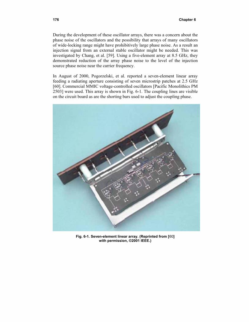
176
During the dephase noise oof wide-lockiinjection signinvestigated demonstratedsource phase In August ofeeding a rad[60]. Comme2503] were uon the circuit
evelopment oof the oscillating range mignal from an by Chang, et
d reduction onoise near th
f 2000, Pogodiating apertuercial MMIC used. This arrt board as are
Fig. 6-1. Sevew
of these oscilltors and the pght have prohexternal stab
t al. [59]. Usiof the array phe carrier freq
orzelski, et aure consistingvoltage-contr
ray is shown ithe shorting
n-element linewith permissi
lator arrays, thpossibility thahibitively largble oscillator ing a five-elephase noise t
quency.
al. reported ag of seven mirolled oscillatin Fig. 6-1. Tbars used to a
ear array. (Repon, ©2001 IEE
here was a coat arrays of m
ge phase noisemight be nement array atto the level o
a seven-elemeicrostrip patctors [Pacific M
The coupling adjust the cou
printed from [EE.)
Chapter
oncern about tmany oscillatoe. As a result
eeded. This wat 8.5 GHz, thof the injecti
ent linear arrches at 2.5 GMonolithics Plines are visib
upling phase.
[60]
r 6
the ors an
was hey ion
ray GHz PM ble
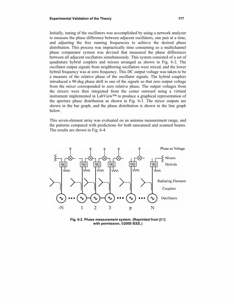
Experimental Validation of the Theory 177
Initially, tuning of the oscillators was accomplished by using a network analyzer to measure the phase difference between adjacent oscillators, one pair at a time, and adjusting the free running frequencies to achieve the desired phase distribution. This process was impractically time consuming so a multichannel phase comparator system was devised that measured the phase differences between all adjacent oscillators simultaneously. This system consisted of a set of quadrature hybrid couplers and mixers arranged as shown in Fig. 6-2. The oscillator output signals from neighboring oscillators were mixed, and the lower hybrid frequency was at zero frequency. This DC output voltage was taken to be a measure of the relative phase of the oscillator signals. The hybrid couplers introduced a 90-deg phase shift in one of the signals so that zero output voltage from the mixer corresponded to zero relative phase. The output voltages from the mixers were then integrated from the center outward using a virtural instrument implemented in LabView™ to produce a graphical representation of the aperture phase distribution as shown in Fig. 6-3. The mixer outputs are shown in the bar graph, and the phase distribution is shown in the line graph below. This seven-element array was evaluated on an antenna measurement range, and the patterns compared with predictions for both unscanned and scanned beams. The results are shown in Fig. 6-4.
Fig. 6-2. Phase measurement system. (Reprinted from [61] with permission, ©2000 IEEE.)
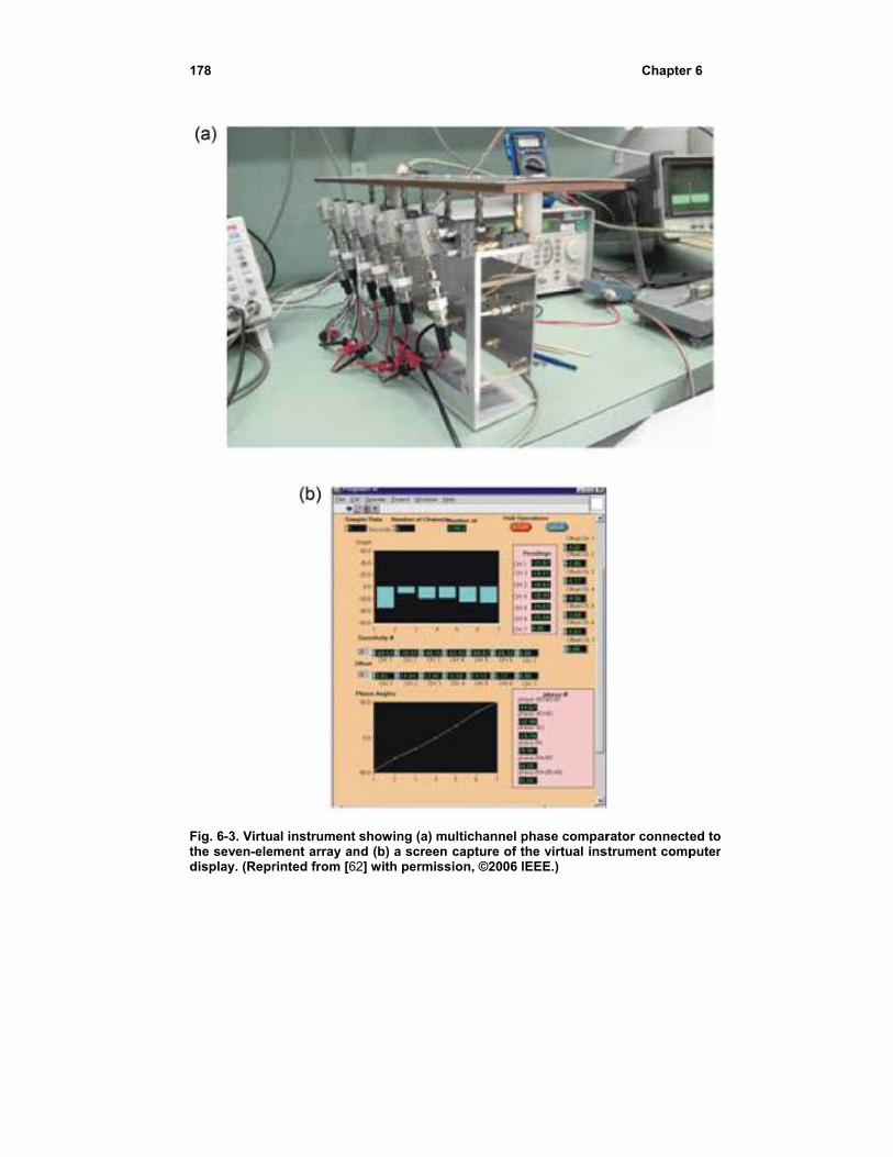
178
Fig. 6-3. Virtuthe seven-eledisplay. (Repr
al instrument ement array anrinted from [6
showing (a) mnd (b) a scree2] with permis
multichannel pn capture of tssion, ©2006 I
phase comparthe virtual insIEEE.)
Chapter
rator connectestrument comp
r 6
ed to puter
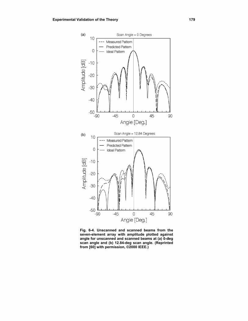
Experimental
Validation of
Fig. 6-4. Useven-elemangle for uscan anglefrom [60] w
the Theory
Unscanned anment array wit
nscanned ande and (b) 12.84with permissio
nd scanned bth amplitude d scanned bea4-deg scan ann, ©2000 IEEE
beams from tplotted again
ams at (a) 0-dngle. (ReprintE.)
17
the nst deg ted
79
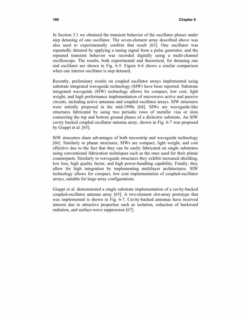
180 Chapter 6
In Section 3.1 we obtained the transient behavior of the oscillator phases under step detuning of one oscillator. The seven-element array described above was also used to experimentally confirm that result [63]. One oscillator was repeatedly detuned by applying a tuning signal from a pulse generator, and the repeated transient behavior was recorded digitally using a multi-channel oscilloscope. The results, both experimental and theoretical, for detuning one end oscillator are shown in Fig. 6-5. Figure 6-6 shows a similar comparison when one interior oscillator is step detuned. Recently, preliminary results on coupled oscillator arrays implemented using substrate integrated waveguide technology (SIW) have been reported. Substrate integrated waveguide (SIW) technology allows for compact, low cost, light weight, and high performance implementation of microwave active and passive circuits, including active antennas and coupled oscillator arrays. SIW structures were initially proposed in the mid-1990s [64]. SIWs are waveguide-like structures fabricated by using two periodic rows of metallic vias or slots connecting the top and bottom ground planes of a dielectric substrate. An SIW cavity backed coupled oscillator antenna array, shown in Fig. 6-7 was proposed by Giuppi et al. [65]. SIW strucutres share advantages of both microstrip and waveguide technology [66]. Similarly to planar structures, SIWs are compact, light weight, and cost effective due to the fact that they can be easily fabricated on single substrates using conventional fabrication techniques such as the ones used for their planar counterparts. Similarly to waveguide structures they exhibit increased shielding, low loss, high quality factor, and high power-handling capability. Finally, they allow for high integration by implementing multilayer architectures. SIW technology allows for compact, low cost implementation of coupled-oscillator arrays, suitable for large array configurations. Giuppi et al. demonstrated a single substrate implementation of a cavity-backed coupled-oscillator antenna array [65]. A two-element slot-array prototype that was implemented is shown in Fig. 6-7. Cavity-backed antennas have received interest due to attractive properties such as isolation, reduction of backward radiation, and surface-wave suppression [67].
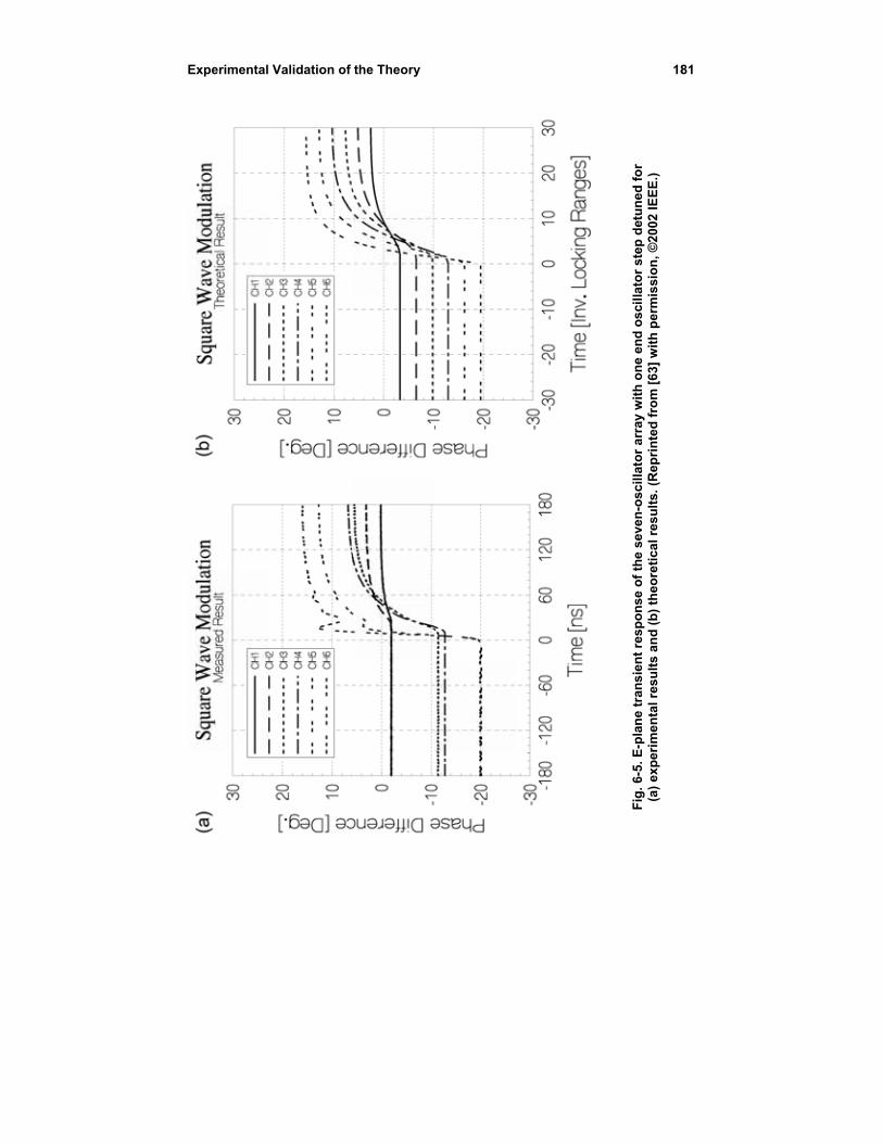
Experimental
Validation of the Theory
18
Fig
. 6-5
. E
-pla
ne
tran
sien
t re
spo
nse
of
the
seve
n-o
scill
ato
r ar
ray
wit
h o
ne
end
osc
illat
or
step
det
un
ed f
or
(a
) ex
per
imen
tal r
esu
lts
and
(b
) th
eore
tica
l re
sult
s. (
Rep
rin
ted
fro
m [
63]
wit
h p
erm
issi
on
, ©20
02 I
EE
E.)
81
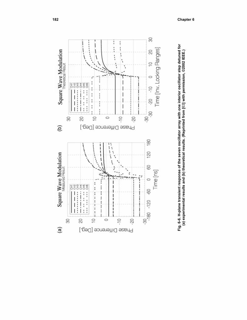
182
Chapter
Fig
. 6-6
. H
-pla
ne
tran
sien
t re
spo
nse
of
the
seve
n o
scill
ato
r ar
ray
wit
h o
ne
inte
rio
r o
scill
ato
r st
ep d
etu
ned
fo
r
(a)
exp
erim
enta
l res
ult
s an
d (
b)
theo
reti
cal r
esu
lts.
(R
epri
nte
d f
rom
[63
] w
ith
per
mis
sio
n, ©
2002
IE
EE
.)
r 6
Experimental
In the work slot-antenna oscillator elestrength is shplaced arounleads to a smsize, compareis less sensiti
Fig. 6-7. Singarray in SIW passive ante2010; used w
Validation of
of Ref. [65], oscillators
ements. The ehown in Fig. nd the middlemoother variat
ed to a singleive to fabricat
gle-substrate technology, anna array. Reith permission
the Theory
SIW technoland addition
effect of the c6-8. It was fo
e of the cavitytion of the coe aperture at ttion tolerance
two-element a) top (active eprinted with n.
logy was usenally controlcoupling aperound that a doy wall, such upling factor he center of t
es.
cavity backecircuit) side,permission f
ed to fabricatl the couplirture size A ouble aperturas the one uas a function
the cavity wa
d coupled os b) bottom (afrom [65]; co
18
te cavity-backing among on the coupl
re symmetricaused in Fig. 6n of the apertuall, and theref
scillator antenantenna) sideopyright EurA
83
ked the ing ally 6-7, ture fore
nna , c)
AAP
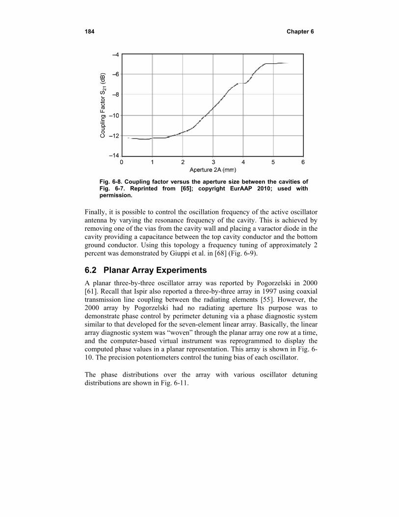
184
Fig. 6-8.Fig. 6-7permiss
Finally, it is antenna by vremoving onecavity providground condpercent was d
6.2 Plan
A planar thr[61]. Recall ttransmission 2000 array demonstrate similar to thaarray diagnosand the comcomputed ph10. The preci The phase distributions
. Coupling fac7. Reprinted sion.
possible to cvarying the ree of the vias fding a capacitductor. Using demonstrated
ar Array E
ree-by-three othat Ispir alsoline couplinby Pogorzelphase contro
at developed fstic system w
mputer-based hase values inision potentio
distributions are shown in
ctor versus thfrom [65];
ontrol the oscesonance freqfrom the cavittance betweenthis topology
d by Giuppi et
Experimen
oscillator arrao reported a tg between thlski had no l by perimetefor the seven-
was “woven” tvirtual instru
n a planar reprometers contro
over the aFig. 6-11.
he aperture sizcopyright E
cillation freququency of thety wall and pn the top caviy a frequencyt al. in [68] (F
nts
ay was reporthree-by-threehe radiating e
radiating aper detuning v-element linethrough the plument was reresentation. Tol the tuning
array with
ze between thEurAAP 2010;
uency of the e cavity. Thislacing a varacity conductory tuning of a
Fig. 6-9).
rted by Pogoe array in 199elements [55]perture Its pia a phase diar array. Basilanar array oneprogrammedThis array is sbias of each o
various osci
Chapter
he cavities of ; used with
active oscillas is achieved ctor diode in r and the bottapproximately
orzelski in 2097 using coax]. However, purpose was agnostic systically, the linne row at a timd to display shown in Fig.oscillator.
illator detun
r 6
f
ator by the
tom y 2
000 xial the to
tem near me, the . 6-
ing
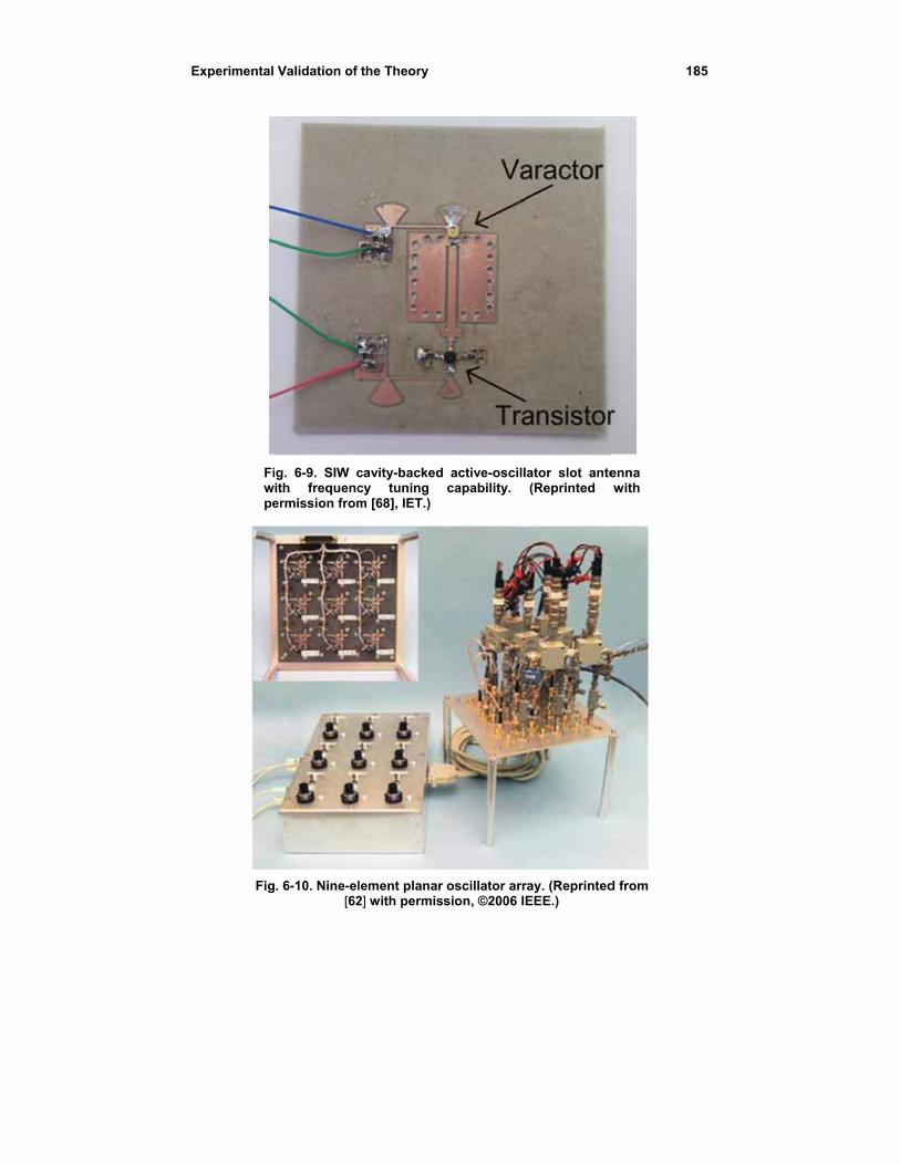
Experimental
Fiwpe
Fig
Validation of
ig. 6-9. SIW cith frequencermission from
. 6-10. Nine-el[62
the Theory
cavity-backedcy tuning m [68], IET.)
lement planar2] with permis
active-oscillacapability.
r oscillator arrssion, ©2006 IE
ator slot ante(Reprinted
ay. (ReprintedEEE.)
18
enna with
d from
85
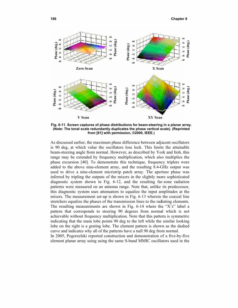
186
Fig. 6-11. Scr(Note: The t
As discussedis 90 deg, atbeam-steerinrange may bphase excursadded to theused to drivinferred by trdiagnostic sypatterns werethis diagnostmixers. The stretchers equThe resultingpattern that achievable windicating thalobe on the rcurve and indIn 2005, Pogelement plan
reen captures onal scale red
from
d earlier, the mt which valug angle from e extended b
sion [40]. To above nine-e a nine-elemripling the ouystem showne measured otic system usmeasurementualize the phag measuremecorresponds
without frequeat the main loright is a gratdicates why agorzelski reponar array using
of phase distdundantly dup
m [61] with per
maximum phaue the oscillat
normal. Howby frequencyo demonstrate-element arrayment micristrutputs of the n in Fig. 6-1on an antennaes attenuatort set-up is shoases of the traents are show
to steering ency multiplicobe points 90ting lobe. Th
all of the patteorted construcg using the sa
ributions for bplicates the phrmission, ©200
ase differencetors lose lock
wever, as descmultiplicatio
e this techniqy, and the rerip patch arramixers in the
12, and the a range. Noters to equalizeown in Fig. 6ansmission linwn in Fig. 6-
90 degrees cation. Note t0 deg to the le element pa
erns have a nuction and demame S-band M
beam-steeringhase vertical s00, IEEE.)
e between adjak. This limitcribed by Yor
on, which alsoque, frequencesulting 8.4-Gay. The apere slightly moresulting far
e that, unlike e the input am6-13 wherein nes to the rad-14 where thefrom norma
that this patteeft while the ttern is show
ull 90 deg frommonstration oMMIC oscilla
Chapter
g in a planar ascale). (Reprin
acent oscillatts the attainark and Itoh, to multiplies cy triplers wGHz output wrture phase wore sophisticar-zone radiatits predecess
mplitudes at the coaxial l
diating elemene “X’s” labe
al which is nern is symmet
similar lookwn as the dash
m normal. of a five-by-fators used in
r 6
array.nted
tors able this the
were was was ated tion sor, the
line nts. el a not tric
king hed
five the
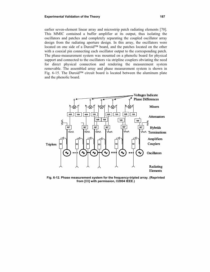
Experimental Validation of the Theory 187
earlier seven-element linear array and microstrip patch radiating elements [70]. This MMIC contained a buffer amplifier at its output, thus isolating the oscillators and patches and completely separating the coupled oscillator array design from the radiating aperture design. In this array, the oscillators were located on one side of a Duroid™ board, and the patches located on the other with a coaxial pin connecting each oscillator output to the corresponding patch. The phase-measurement system was mounted on a phenolic board for physical support and connected to the oscillators via stripline couplers obviating the need for direct physical connection and rendering the measurement system removable. The assembled array and phase measurement system is shown in Fig. 6-15. The Duroid™ circuit board is located between the aluminum plate and the phenolic board.
Fig. 6-12. Phase measurement system for the frequency-tripled array. (Reprinted from [69] with permission, ©2004 IEEE.)
Oscillators
90° 90°90° 90° 90° 90°
Mixers
Voltages Indicate Phase Differences
Hybrids
CouplersX3 X3X3X3 X3 X3
Amplifiers
Triplers
0dB 7dB0dB 0dB 0dB 7dB7dB7dB
7dB0dB7dB7dB
Attenuators
Radiating Elements
Terminations
rfrfrf rf rflo lo lo lo lo
Oscillators
90° 90°90° 90° 90° 90°
Mixers
Voltages Indicate Phase Differences
Hybrids
CouplersX3 X3X3X3 X3 X3
Amplifiers
Triplers
0dB 7dB0dB 0dB 0dB 7dB7dB7dB
7dB0dB7dB7dB
Attenuators
Radiating Elements
Terminations
rfrfrf rf rflo lo lo lo lo
Oscillators
90° 90°90° 90° 90° 90°
Mixers
Voltages Indicate Phase Differences
Hybrids
CouplersX3X3 X3X3X3X3X3X3 X3X3 X3X3
Amplifiers
Triplers
0dB 7dB0dB 0dB 0dB 7dB7dB7dB
7dB0dB7dB7dB
Attenuators
Radiating Elements
Terminations
rfrfrf rf rflo lo lo lo lo
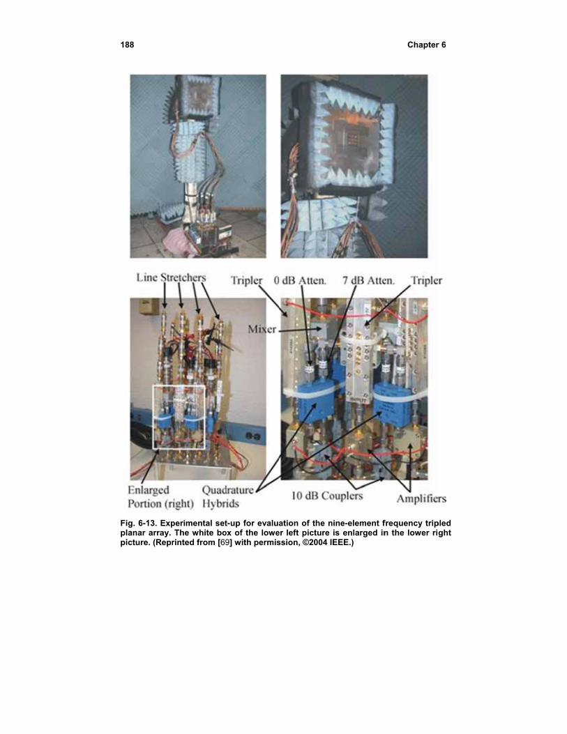
188
Fig. 6-13. Expplanar array. picture. (Repr
perimental setThe white bo
rinted from [69
t-up for evaluox of the lowe9] with permis
ation of the ner left picture ssion, ©2004 I
nine-element fis enlarged inEEE.)
Chapter
frequency tripn the lower ri
r 6
pled ght
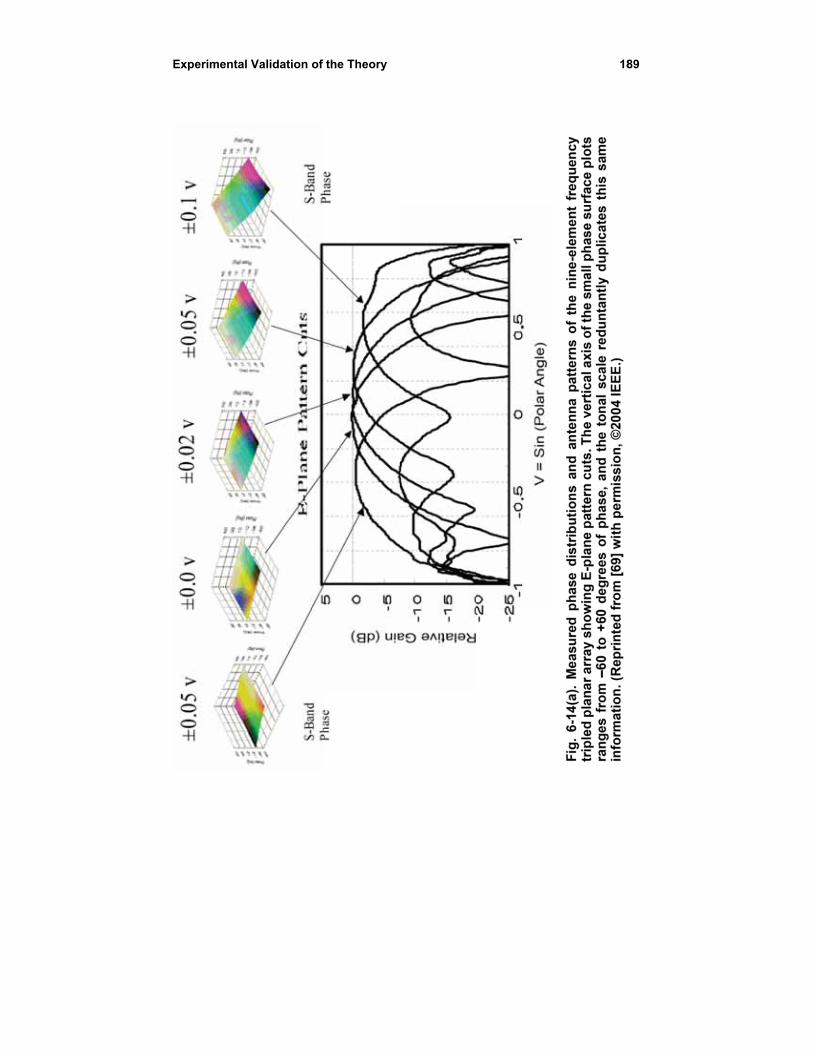
Experimental
Validation of the Theory
1889
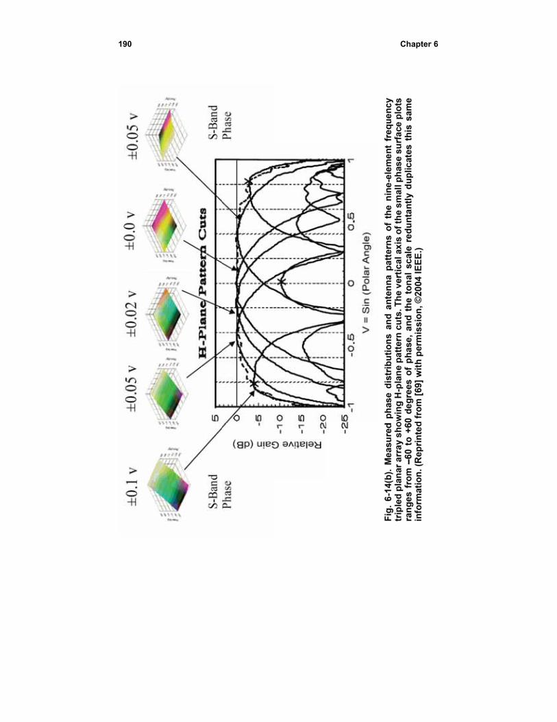
190
Chapterr 6
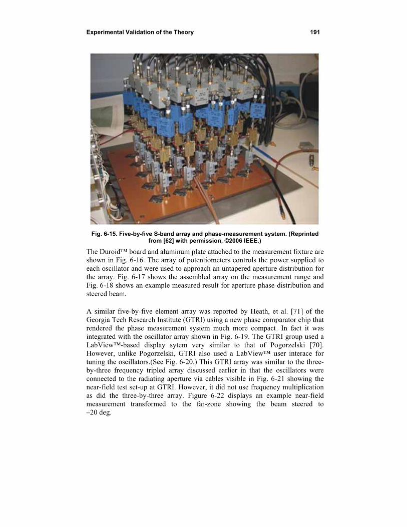
Experimental
Fig. 6-15. Fi
The Duroid™shown in Figeach oscillatothe array. FigFig. 6-18 shosteered beam A similar fivGeorgia Techrendered theintegrated wiLabView™-bHowever, untuning the osby-three freqconnected tonear-field tesas did the tmeasurement–20 deg.
Validation of
ve-by-five S-bfrom
™ board and ag. 6-16. The aor and were ug. 6-17 showows an examp
m.
ve-by-five eleh Research In phase measith the oscillabased displaynlike Pogorzescillators.(Seequency triple the radiating
st set-up at Gthree-by-threet transforme
the Theory
band array and[62] with perm
aluminum plaarray of potenused to appro
ws the assembple measured
ement array wnstitute (GTRurement syst
ator array shoy sytem verelski, GTRI ae Fig. 6-20.) Td array discug aperture via
GTRI. Howevee array. Figud to the fa
d phase-measmission, ©200
ate attached tontiometers coach an untap
bled array on result for ap
was reported I) using a newtem much mown in Fig. 6ry similar toalso used a LThis GTRI arussed earlier a cables visiber, it did not ure 6-22 dispar-zone show
surement syst06 IEEE.)
o the measureontrols the poered aperturethe measure
erture phase
by Heath, etw phase comp
more compact.-19. The GTR
o that of PoLabView™ urray was simiin that the o
ble in Fig. 6-use frequenc
plays an exawing the be
19
tem. (Reprinte
ement fixture ower suppliede distribution ement range adistribution a
t al. [71] of parator chip t. In fact it wRI group useogorzelski [7user interace ilar to the throscillators w-21 showing cy multiplicatample near-fieam steered
91
ed
are d to for
and and
the that was d a
70]. for
ree-were
the ion ield
to
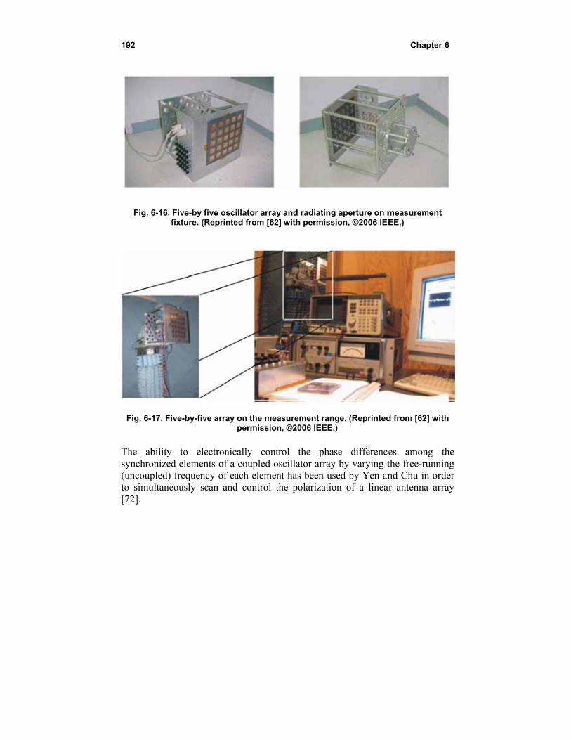
192
Fig. 6-16. Ff
Fig. 6-17. Fiv
The ability synchronized(uncoupled) to simultaneo[72].
Five-by five osixture. (Reprin
ve-by-five arra
to electrond elements of frequency of ously scan a
scillator array nted from [62]
ay on the meapermission
nically contrf a coupled osf each elemennd control th
and radiating with permiss
asurement rann, ©2006 IEEE.
rol the phascillator arraynt has been ushe polarizatio
g aperture on msion, ©2006 IE
ge. (Reprinted.)
se differency by varying tsed by Yen anon of a linea
Chapter
measurementEE.)
d from [62] wit
ces among the free-runnnd Chu in or
ar antenna arr
r 6
t
th
the ing
rder ray
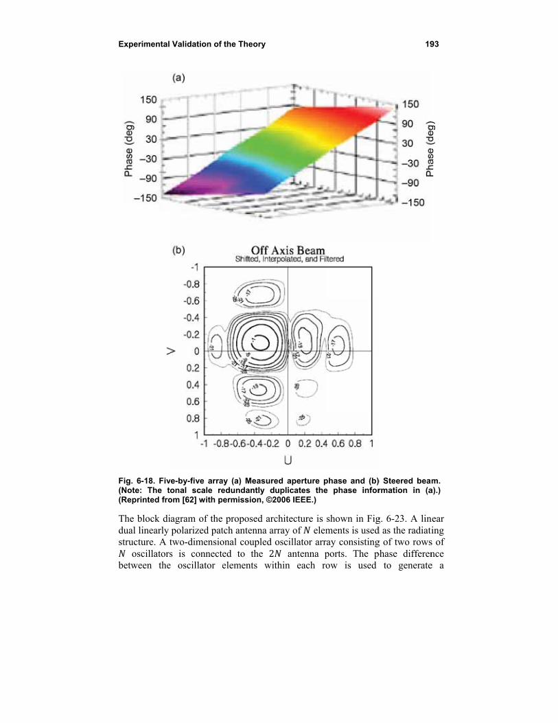
Experimental
Fig. 6-18. Fiv(Note: The t(Reprinted fro
The block didual linearly structure. A t
oscillatorsbetween the
Validation of
ve-by-five arraonal scale reom [62] with p
iagram of thepolarized pattwo-dimensios is connect
e oscillator e
the Theory
ay (a) Measureedundantly d
permission, ©2
proposed arctch antenna aronal coupled ed to the 2elements wit
ed aperture puplicates the
2006 IEEE.)
chitecture is rray of elemoscillator arra
antenna pthin each ro
phase and (b)e phase infor
shown in Figments is useday consistingports. The pow is used
19
) Steered bearmation in (a
g. 6-23. A lind as the radiatg of two rowsphase differen
to generate
93
m. a).)
near ting s of nce e a
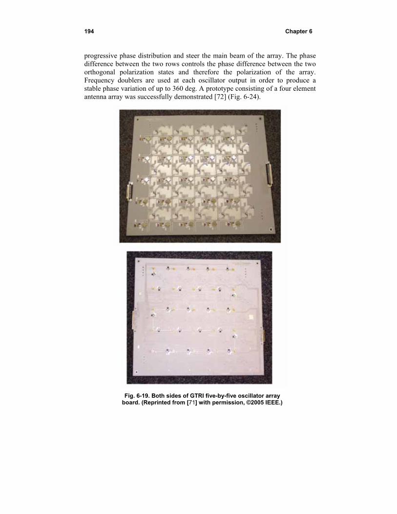
194
progressive pdifference beorthogonal pFrequency dstable phase vantenna array
phase distribuetween the twpolarization
doublers are uvariation of uy was success
Fig. 6-19. Boboard. (Repri
ution and steewo rows contr
states and tused at eachup to 360 degsfully demons
oth sides of GTnted from [71
er the main brols the phaseherefore the oscillator ou. A prototype
strated [72] (F
TRI five-by-fiv] with permiss
beam of the ae difference b
polarizationutput in orde
e consisting oFig. 6-24).
ve oscillator arsion, ©2005 IE
Chapter
array. The phbetween the tn of the arrer to produce
of a four elem
rray EEE.)
r 6
hase two ray. e a
ment
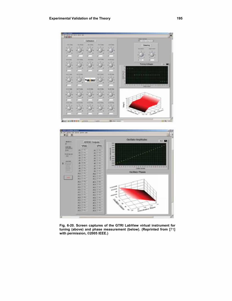
Experimental
Fig. 6-2tuning with pe
Validation of
20. Screen ca(above) and
ermission, ©20
the Theory
ptures of the phase measu005 IEEE.)
GTRI LabVieurement (below
ew virtual instw). (Reprinted
19
trument for d from [71]
95
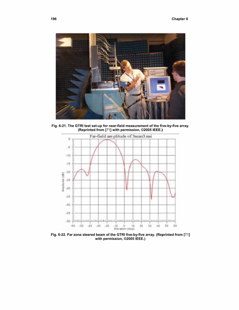
196
Fig. 6-21. The
Fig. 6-22. Far
e GTRI test se(Reprinted
zone steered w
et-up for near-f from [71] wit
beam of the Gwith permissi
field measureh permission,
GTRI five-by-fon, ©2005 IEE
ment of the fiv ©2005 IEEE.)
ive array. (RepEE.)
Chapter
ve-by-five arra)
printed from [
r 6
ay.
[71]
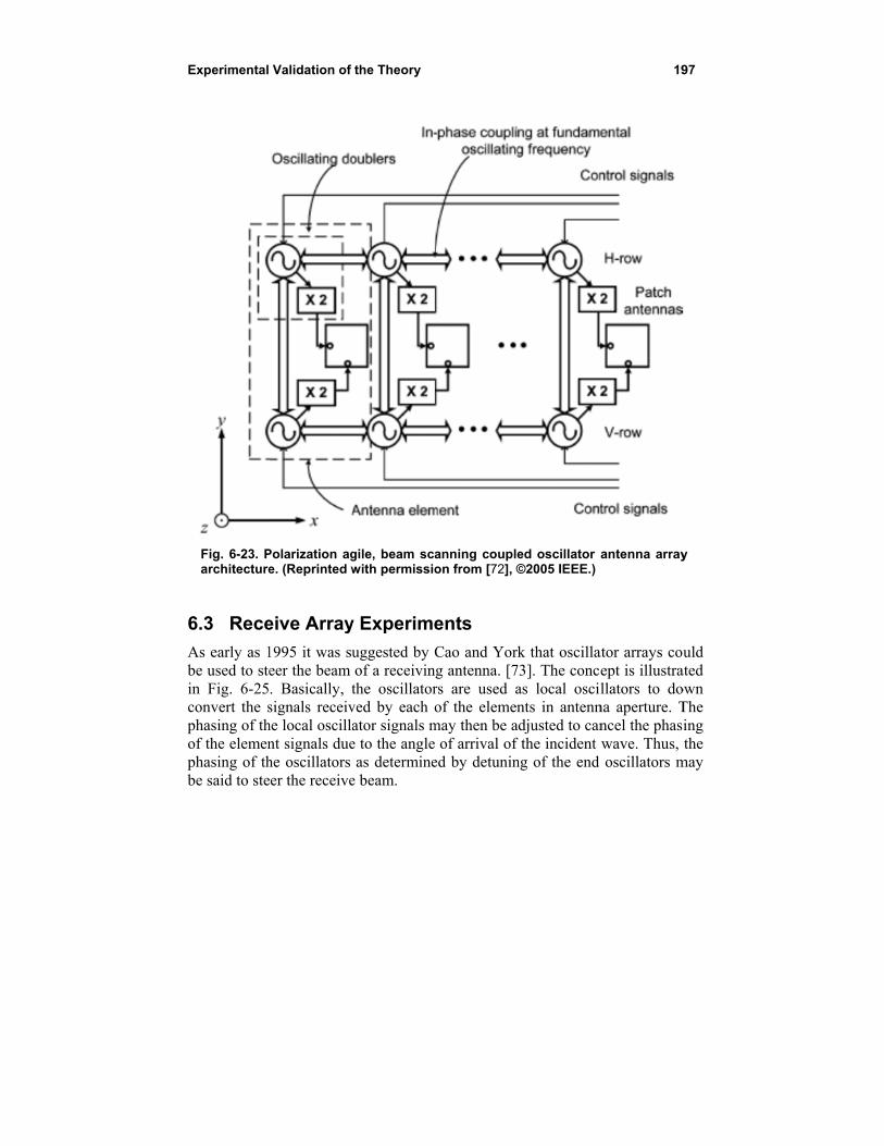
Experimental
Fig. 6-23. Parchitecture
6.3 Rece
As early as 1be used to stein Fig. 6-25convert the sphasing of thof the elemenphasing of thbe said to ste
Validation of
Polarization age. (Reprinted w
eive Array
1995 it was sueer the beam . Basically, tsignals receivhe local oscillant signals duehe oscillators eer the receive
the Theory
gile, beam scawith permissio
y Experime
uggested by Cof a receivinthe oscillatorved by each oator signals me to the angleas determine
e beam.
anning coupleon from [72], ©
ents
Cao and Yorkng antenna. [7rs are used aof the elemen
may then be a of arrival of
ed by detunin
ed oscillator ©2005 IEEE.)
k that oscilla73]. The concas local oscilnts in antenn
adjusted to canf the incident ng of the end
19
antenna array
ator arrays couept is illustrallators to do
na aperture. Tncel the phaswave. Thus, oscillators m
97
y
uld ated own The ing the
may
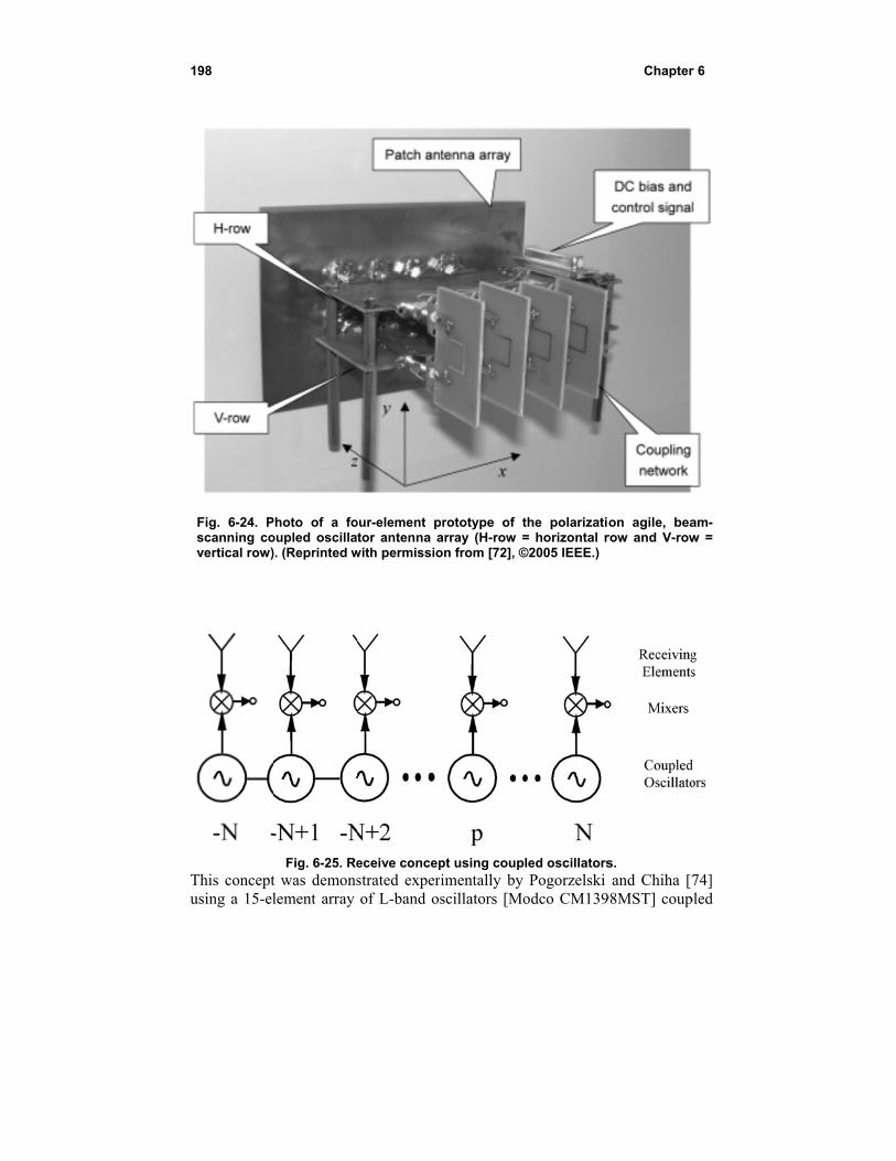
198
Fig. 6-24. Pscanning covertical row)
This conceptusing a 15-el
Photo of a fooupled oscilla). (Reprinted w
Fig. 6-25. Ret was demonslement array
our-element ptor antenna a
with permissio
eceive concepstrated experiof L-band os
prototype of tarray (H-row =on from [72], ©
pt using coupimentally by scillators [Mo
the polarizatio= horizontal r©2005 IEEE.)
led oscillatorsPogorzelski
odco CM139
Chapter
on agile, bearow and V-row
s. and Chiha [7
98MST] coup
r 6
am-w =
74] pled
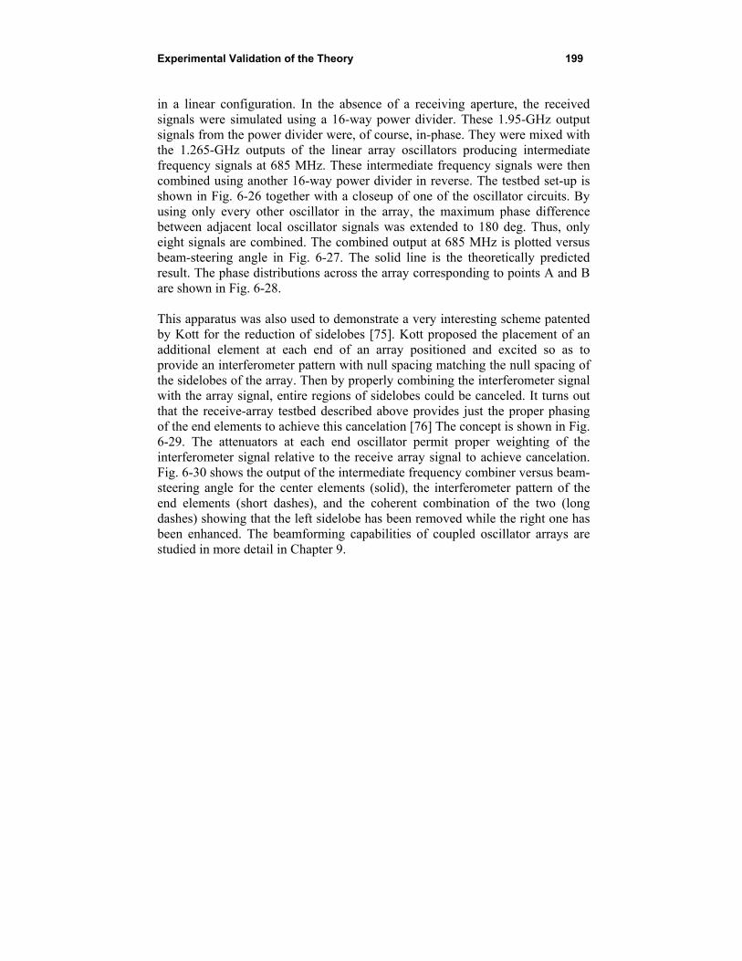
Experimental Validation of the Theory 199
in a linear configuration. In the absence of a receiving aperture, the received signals were simulated using a 16-way power divider. These 1.95-GHz output signals from the power divider were, of course, in-phase. They were mixed with the 1.265-GHz outputs of the linear array oscillators producing intermediate frequency signals at 685 MHz. These intermediate frequency signals were then combined using another 16-way power divider in reverse. The testbed set-up is shown in Fig. 6-26 together with a closeup of one of the oscillator circuits. By using only every other oscillator in the array, the maximum phase difference between adjacent local oscillator signals was extended to 180 deg. Thus, only eight signals are combined. The combined output at 685 MHz is plotted versus beam-steering angle in Fig. 6-27. The solid line is the theoretically predicted result. The phase distributions across the array corresponding to points A and B are shown in Fig. 6-28. This apparatus was also used to demonstrate a very interesting scheme patented by Kott for the reduction of sidelobes [75]. Kott proposed the placement of an additional element at each end of an array positioned and excited so as to provide an interferometer pattern with null spacing matching the null spacing of the sidelobes of the array. Then by properly combining the interferometer signal with the array signal, entire regions of sidelobes could be canceled. It turns out that the receive-array testbed described above provides just the proper phasing of the end elements to achieve this cancelation [76] The concept is shown in Fig. 6-29. The attenuators at each end oscillator permit proper weighting of the interferometer signal relative to the receive array signal to achieve cancelation. Fig. 6-30 shows the output of the intermediate frequency combiner versus beam-steering angle for the center elements (solid), the interferometer pattern of the end elements (short dashes), and the coherent combination of the two (long dashes) showing that the left sidelobe has been removed while the right one has been enhanced. The beamforming capabilities of coupled oscillator arrays are studied in more detail in Chapter 9.
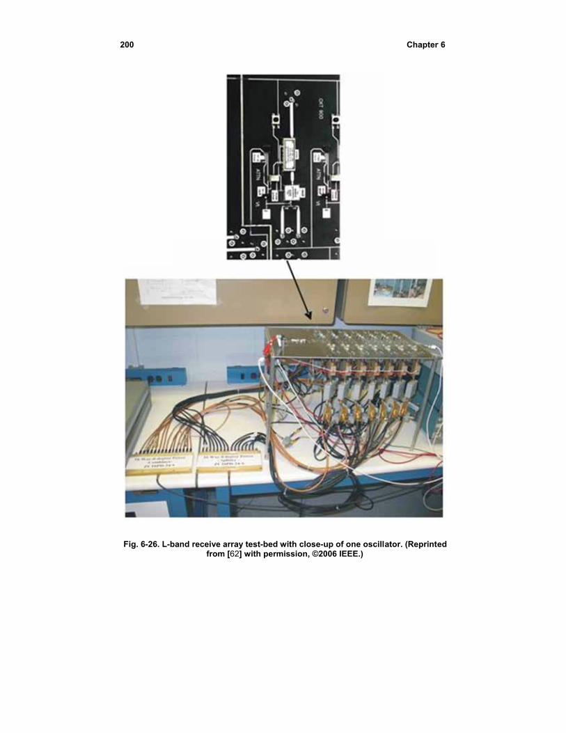
200
Fig. 6-26. L-b
band receive afrom
array test-bed [62] with perm
with close-upmission, ©200
p of one oscill06 IEEE.)
Chapter
ator. (Reprinte
r 6
ed
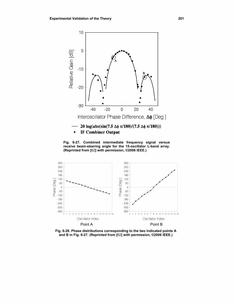
Experimental Validation of the Theory 201
Fig. 6-27. Combined intermediate frequency signal versus receive beam-steering angle for the 15-oscillator L-band array. (Reprinted from [62] with permission, ©2006 IEEE.)
Point A Point B
Fig. 6-28. Phase distributions corresponding to the two indicated points A and B in Fig. 6-27. (Reprinted from [62] with permission, ©2006 IEEE.)
A
B
A
B
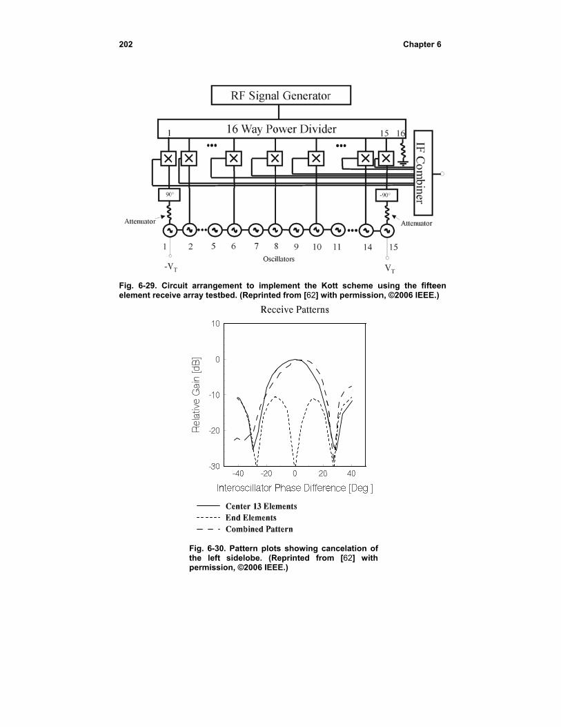
202
Fig. 6-29. Cirelement recei
rcuit arrangemive array testb
Fig. 6-30the left permissio
ment to implbed. (Reprinte
. Pattern plotsidelobe. (R
on, ©2006 IEE
ement the Kod from [62] wi
ts showing caReprinted fromEE.)
ott scheme uith permission
ancelation of m [62] with
Chapter
using the fiften, ©2006 IEEE
r 6
een
E.)

Experimental
It should be rreceive posesarray, the oschybrid frequeoscillator phaarray elemenconjugate of using the oscfrequency wcombining fofrequency rat
In closing thioscillating ma coupled osbeen used in [77]. Additioapplications [79]. The arra
The SOM elethe necessar
Validation of
recognized ths a certain cocillator signalency of the mases are subt
nts. The resulf the phasing cillator signa
were combineor receive wother than at a
is section on mixers when pscillator arrayretro-directiv
onally, the uhas been invay topology p
Fig. 6-31
ement consisry feedback
the Theory
hat using the somplexity. Thls are used to
mixers that is ctracted from lt is that the required to t
als to excite ted on receiveould then be d
low intermed
receive arrayproperly coupy. Coupled seve array applicuse of couplevestigated by proposed in R
1. Coupled sel(Copyright ©2ts of an amplto obtain th
same oscillatohis is true bec
down convercombined to the phases oreceive phas
transmit a bethe elements.e, this woulddone at approdiate frequenc
ys it should bpled is synchrelf-oscillatingcations such aed SOM arra
Sanagi et alRef. [78] is sho
f-oscillating m2005 IEICE [78lifier and a b
he oscillation
or array for bocause in the prt the signal, sproduce the o
of the signals sing of the oam in the sam If instead thd not be the
oximately twicy.
e noted that aronized in freg mixer (SOMas the work bays in receivl. [78] and vown in Fig. 6
mixer array. 8].) ranch line co
n. A varacto
20
oth transmit aproposed receso it is the lowoutput. Thus received at
oscillators is me direction he upper hybe case, but ce the oscilla
an array of seequency formM) arrays haby Shiroma etve phased-arrver Hoeye et 6-31.
oupler providor diode in
03
and eive wer the the the by
brid the
ator
elf-ming
ave t al. rray
al.
ding the
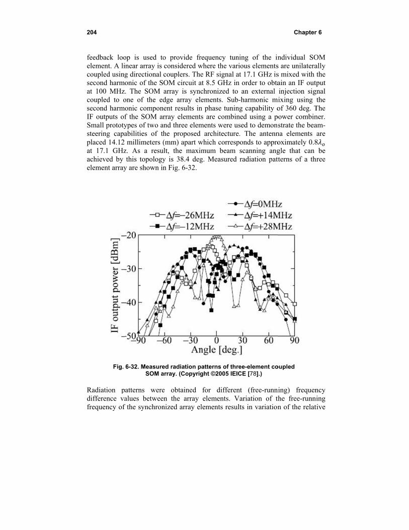
204
feedback looelement. A licoupled usingsecond harmat 100 MHzcoupled to osecond harmIF outputs ofSmall prototysteering capaplaced 14.12at 17.1 GHzachieved by element array
Fig.
Radiation pdifference vafrequency of
op is used toinear array is g directional onic of the S. The SOM one of the ed
monic componf the SOM arypes of two aabilities of t millimeters (z. As a resuthis topology
y are shown in
6-32. MeasureSOM a
patterns werealues betweef the synchron
o provide frconsidered wcouplers. TheOM circuit aarray is syncdge array ele
nent results inrray elements
and three elemhe proposed (mm) apart w
ult, the maximy is 38.4 degn Fig. 6-32.
ed radiation parray. (Copyrig
e obtained en the array nized array el
requency tuniwhere the varie RF signal atat 8.5 GHz in chronized to ements. Sub-
n phase tunings are combin
ments were usarchitecture.
which correspmum beam g. Measured
atterns of threght ©2005 IEIC
for differenelements. V
lements resul
ing of the inious elementst 17.1 GHz isorder to obtaan external
-harmonic mg capability o
ned using a psed to demon. The antennonds to approscanning angradiation pat
ee-element coCE [78].)
nt (free-runnariation of thts in variation
Chapter
ndividual SOs are unilateras mixed with ain an IF outpinjection sig
mixing using of 360 deg. T
power combinnstrate the beana elements oximately 0.8gle that can tterns of a th
oupled
ning) frequenthe free-runnn of the relat
r 6
OM ally the
tput gnal
the The ner. am-are
8 be
hree
ncy ing tive
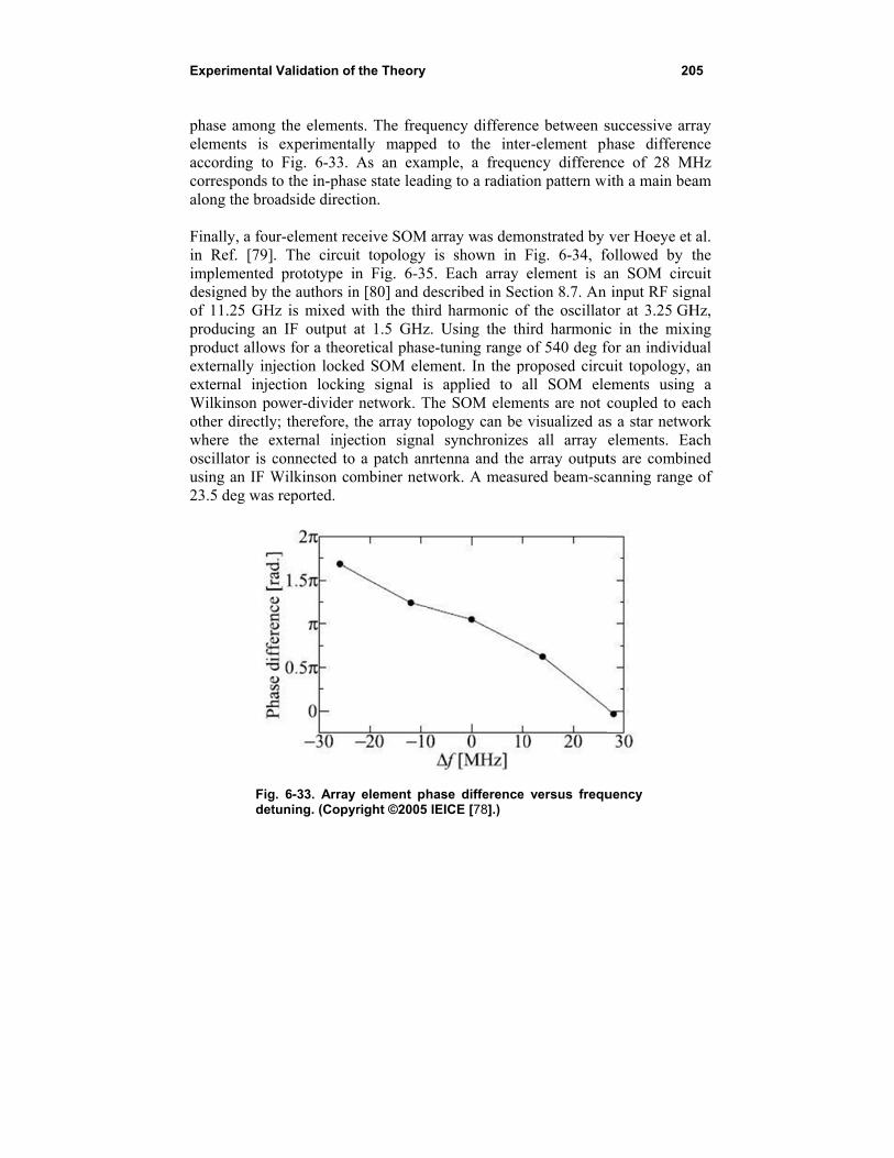
Experimental
phase amongelements is according tocorresponds talong the bro Finally, a fouin Ref. [79]implementeddesigned by tof 11.25 GHproducing anproduct allowexternally injexternal injeWilkinson poother directlywhere the eoscillator is cusing an IF W23.5 deg was
Figdet
Validation of
g the elementexperimenta
o Fig. 6-33. to the in-phas
oadside direct
ur-element rec. The circuit
d prototype inthe authors in
Hz is mixed wn IF output aws for a theorjection locke
ection lockinower-divider y; therefore, texternal injecconnected to Wilkinson cos reported.
g. 6-33. Array tuning. (Copy
the Theory
ts. The frequeally mapped As an examse state leadinion.
ceive SOM art topology isn Fig. 6-35. n [80] and deswith the thirdat 1.5 GHz. retical phase-d SOM elem
ng signal is network. The
the array topoction signal a patch anrt
ombiner netwo
element pharight ©2005 IE
ency differento the inte
ple, a frequeng to a radiati
rray was dems shown in Each array
scribed in Secd harmonic oUsing the thtuning range
ment. In the papplied to ae SOM elemology can be synchronizes
enna and theork. A measu
ase differenceEICE [78].)
nce between ser-element phency differenion pattern wi
monstrated by Fig. 6-34, foelement is a
ction 8.7. An f the oscillat
hird harmonicof 540 deg f
proposed circuall SOM eleents are not cvisualized as
s all array array output
ured beam-sc
e versus frequ
20
successive arrhase differen
nce of 28 Mith a main be
ver Hoeye etfollowed by an SOM circinput RF sig
tor at 3.25 GHc in the mixfor an individuit topology, ements usingcoupled to eas a star netwoelements. Eats are combinanning range
uency
05
ray nce
MHz eam
t al. the
cuit gnal Hz, ing
dual an
g a ach ork ach ned e of
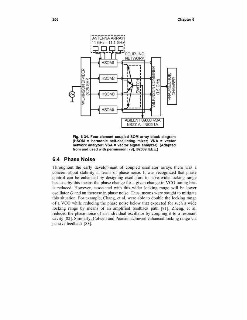
206
Fi(Hnefr
6.4 Phas
Throughout concern aboucontrol can bbecause by this reduced. Hoscillator Q athis situationof a VCO whlocking rangreduced the pcavity [82]. Spassive feedb
ig. 6-34. FourHSOM = harmetwork analyz
rom and used
se Noise
the early deut stability inbe enhanced his means theHowever, assand an increa
n. For examplhile reducing
ge by means phase noise oSimilarly, Colback [83].
r-element coumonic self-oszer; VSA = vewith permissi
evelopment on terms of phby designing
e phase changsociated withse in phase nole, Chang, et g the phase no
of an amplof an individulwell and Pea
pled SOM arrcillating mixector signal anion [79], ©200
of coupled oshase noise. Itg oscillators ge for a givenh this wider loise. Thus, mal. were ableoise below thlified feedbacual oscillator arson achieved
ray block diager; VNA = venalyzer). (Ada9 IEEE.)
scillator arrat was recognto have wide
n change in Vlocking range
means were soe to double thhat expected ck path [81]by coupling
d enhanced lo
Chapter
gram ector apted
ays there wasnized that phe locking ran
VCO tuning be will be low
ought to mitighe locking ranfor such a w]. Zheng, et it to a reson
ocking range
r 6
s a ase nge bias wer gate nge
wide al.
nant via
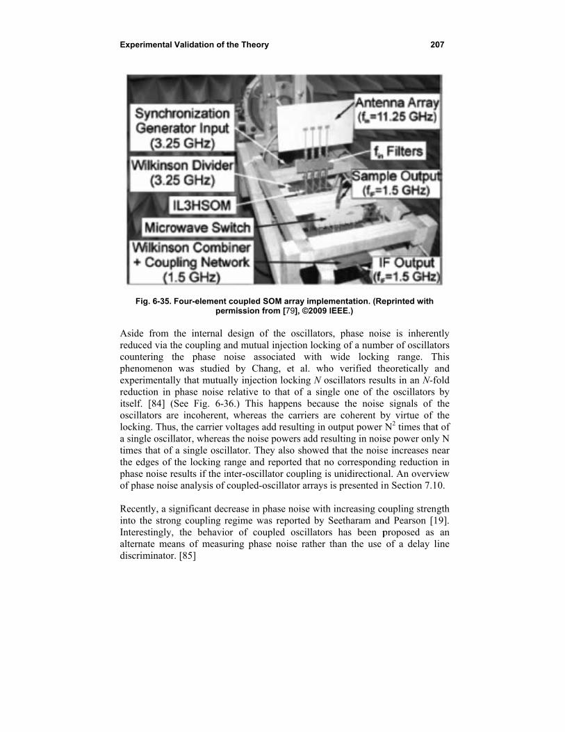
Experimental
Fig. 6-35.
Aside from reduced via tcountering tphenomenonexperimentalreduction in itself. [84] (oscillators arlocking. Thua single osciltimes that of the edges of phase noise rof phase nois Recently, a sinto the stronInterestingly,alternate meadiscriminator
Validation of
Four-elementpe
the internal the coupling athe phase n was studiedlly that mutuaphase noise
(See Fig. 6-3re incoherents, the carrier llator, whereaf a single osci
the locking rresults if the ise analysis of
ignificant decng coupling r, the behavioans of measur. [85]
the Theory
t coupled SOMrmission from
design of thand mutual innoise associd by Changally injection relative to th
36.) This hat, whereas thvoltages add
as the noise poillator. They range and repinter-oscillato
f coupled-osci
crease in phasregime was ror of coupleuring phase n
M array implemm [79], ©2009 I
he oscillatorsnjection lockiniated with wg, et al. who
locking N oshat of a sing
appens becauhe carriers arresulting in o
owers add resalso showed ported that noor coupling isillator arrays i
se noise with reported by Sed oscillatorsnoise rather t
mentation. (ReIEEE.)
s, phase noisng of a numbwide lockino verified thscillators resugle one of thse the noise
re coherent boutput power sulting in noisthat the noise
o correspondis unidirectionais presented in
increasing coSeetharam ans has been pthan the use
20
eprinted with
se is inherenber of oscillatng range. Theoretically aults in an N-fhe oscillators e signals of by virtue of N2 times that
se power onlye increases ning reductional. An overvin Section 7.1
oupling strennd Pearson [1proposed as of a delay l
07
ntly tors
This and fold
by the the t of y N near n in iew 0.
ngth 19].
an line
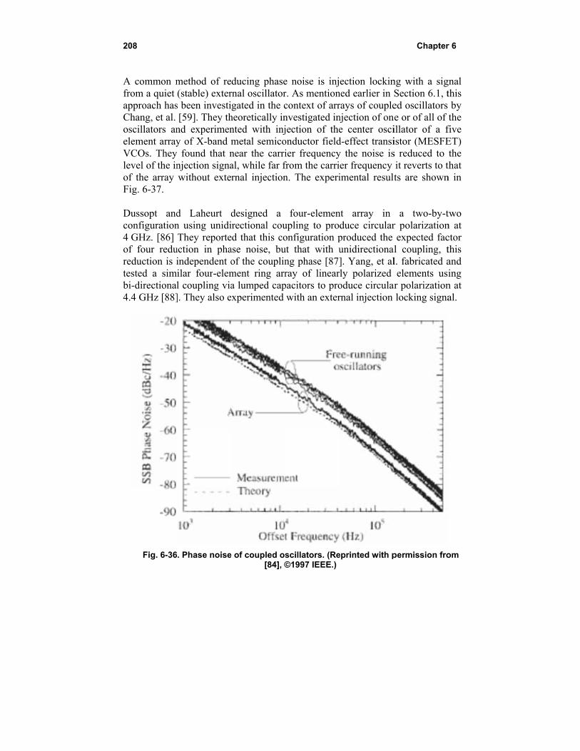
208
A common mfrom a quiet approach hasChang, et al. oscillators anelement arrayVCOs. Theylevel of the inof the array Fig. 6-37. Dussopt andconfiguration4 GHz. [86]of four redureduction is itested a simbi-directional4.4 GHz [88]
Fig. 6-36
method of re(stable) exter
s been investi[59]. They th
nd experimeny of X-band m
y found that nnjection signawithout exte
d Laheurt dn using unidiThey reporte
uction in phaindependent oilar four-eleml coupling via]. They also e
6. Phase noise
ducing phasernal oscillatorgated in the c
heoretically innted with injmetal semiconear the carrial, while far frnal injection
designed a irectional coued that this coase noise, buof the couplinment ring arra lumped cap
experimented
e of coupled os[84], ©
e noise is injr. As mentioncontext of arrnvestigated injection of theonductor fieldier frequencyfrom the carrin. The experi
four-elemenupling to proonfiguration put that with ung phase [87]ray of linear
pacitors to prowith an exter
scillators. (Re©1997 IEEE.)
ection lockinned earlier in rays of couplenjection of one center oscid-effect transiy the noise iser frequency imental result
nt array in duce circularproduced the unidirectiona]. Yang, et al
rly polarized oduce circularnal injection
eprinted with p
Chapter
ng with a sigSection 6.1, ted oscillators
ne or of all of illator of a fistor (MESFEs reduced to it reverts to tts are shown
a two-by-tr polarizationexpected fac
al coupling, tl. fabricated aelements us
ar polarizationlocking signa
permission fro
r 6
gnal this by the
five ET) the
that n in
two n at ctor this and ing n at al.
om
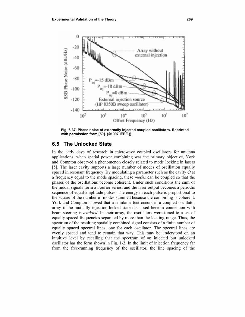
Experimental
Fig. 6-37with per
6.5 The U
In the early applications, and Compton[5]. The lasespaced in resa frequency ephases of thethe modal sigsequence of ethe square ofYork and Coarray if the mbeam-steerinequally spacespectrum of tequally spacevenly spaceintuitive levoscillator hasfrom the fre
Validation of
7. Phase noisermission from
Unlocked
days of reswhen spatia
n observed a er cavity supponant frequenequal to the me oscillationsgnals form a Fequal-amplituf the number ompton showmutually injeg is avoided.ed frequenciethe resulting sced spectral led and tend el by recallis the form shoee-running fr
the Theory
e of externally[59]. (©1997 I
State
search in mical power comphenomenonports a large ncy. By modumode spacing become cohFourier seriesude pulses. Thof modes sum
wed that a simection-locked. In their arraes separated bspatially comlines, one foto remain thing that the own in Fig. 1requency of
y injected couEEE.))
crowave coupmbining was tn closely relat
number of mulating a parag, these modeherent. Unders, and the lasehe energy in mmed becaus
milar effect ocd state discusay, the oscillby more than
mbined signal cr each oscill
hat way. Thisspectrum of
1-2. In the limthe oscillato
pled oscillato
pled oscillatothe primary ted to mode lmodes of osc
ameter such ases can be cour such conditier output beceach pulse is
se the combinccurs in a cosed here in clators were tuthe locking r
consists of a flator. The sps may be unf an injected
mit of injectioor, the line
20
rs. Reprinted
ors for antenobjective, Yo
locking in lascillation equas the cavity Q
upled so that ions the sum
comes a perios proportionalning is cohereoupled oscillaconnection wuned to a setrange. Thus, finite number
pectral lines nderstood on d but unlockon frequency spacing of
09
nna ork sers ally Q at the
m of odic l to ent. ator with t of the r of are an
ked far the
210 Chapter 6
unlocked spectrum is approximately equal to the difference between the injection frequency and the free-running frequency. That is,
2 2inj lock inj (6.5-1)
Thus, because the injection signals come from the nearest neighbors, this means that the line spacing of the unlocked spectra is approximately equal to the difference in the free-running frequencies of the neighboring oscillators. In effect then, the oscillators each lock to a line of the unlocked spectrum of their neighbors, and the line spacing of the array becomes uniform. The stability of such mode-locked states has been studied in some detail by Lynch and York [89]. Note that as the differences in the tuning of the neighboring oscillators approach the locking range, the approximation Eq. (6.5-1) fails, the line spacing approaches zero, and the array becomes mutually injection locked, producing a monochromatic output. Maintenance of the mode-locked condition requires that mutual injection locking be avoided. As described in Section 1.4, the locking range can be controlled by adjusting the coupling phase, and in fact, if the coupling phase is 90 deg, the locking range becomes zero, and mutual injection locking is precluded. Thus, from a mode-locking perspective, a 90-deg coupling phase is to be preferred as noted by Lynch and York [89] [90]. One may view the finite line spectrum of the combined output as an infinite line spectrum filtered by a bandpass filter passing only the lines corresponding to the range of oscillator tunings. From Fourier theory, the corresponding time function will be an infinite sequence of equally spaced pulses whose shape is the inverse Fourier transform of the filter bandpass characteristic. For example, if the filter is a square pulse in frequency, the temporal pulses will be sinc functions. York and Compton demonstrated this with an array of three oscillators [5]. A few months later, York and Compton published additional results showing that, when a mode-locked array of oscillators is used to feed a linear array of radiating elements, the resulting beam scans as a function of time [6]. This is a consequence of the fact that the radiating elements are fed with slightly differing frequencies. The frequency differences may be viewed as relative phases changing linearly with time. Thus, the inter-element phasing of the array of elements changes linearly with time, resulting in a beam that scans with time. The repetition rate of the scan is just the period of the pulse output of the array, and at any given angle in the far-zone pattern, the received signal will repeat temporally with this same period as the beam repeatedly scans past that angle.
Experimental Validation of the Theory 211
More recently, the unlocked state of such arrays has been studied as a generator of a chaotic output signal. The array is controlled by modulation of the coupling parameters with the objective of embedding information in the transitioning of the signal between the various unstable periodic orbits [91]. As indicated by York and Itoh [40], all of the phenomena observed for coupled voltage controlled oscillators (VCOs) may also be produced by coupled phase-locked loops (PLLs); one merely has more design flexibility when using PLLs. Section 7.12 contains an introduction to the analysis of coupled phase-locked loops. These principles were demonstrated in a two-element array by Martinez and Compton [92]. This also holds true for mode-locked arrays [93].
6.6 Conclusion
In this chapter we have outlined the experimental work leading to the current level of understanding of the design and fabrication of coupled-oscillator arrays and associated radiating apertures and their performance characteristics. Of course the work has continued as we write, and much of the most recent work severely taxes the capabilities of the linear approximation in explaining the results. Thus, the current trend favors full nonlinear design and analysis. While more complex, such an approach more accurately describes the expected behavior and permits exploitation of the nonlinear effects. These are aspects discussed in Part III of this book.

212 Chapter 6
213
Part III: Nonlinear Behavior
Chapter 7 Perturbation Models for Stability, Phase
Noise, and Modulation
The complex dynamics of coupled-oscillator arrays lead to the existence of a multitude of steady-state solutions. In addition to finding or selecting a desired steady-state solution, one further needs to guarantee its stability. In this section, perturbation methods are described that allow the designer to examine both the existence as well as the local stability of the various steady-state solutions of coupled oscillator arrays. An introduction to stability analysis of nonlinear dynamical systems is presented [94], followed by its application to coupled oscillator systems [95] [96]. The perturbation nature of noise, leads to phase-noise analysis methods that are closely related to the formulation used in the stability analysis. Analytical models are presented that demonstrate the attractive properties of coupled inter-injection locked oscillator systems, among them improved phase-noise performance compared to single elements [97]. A straightforward application of coupled-oscillator arrays has been in power-combining arrays where, by controlling the phase shift within an array of synchronized oscillator elements, one can direct the radiated beam towards a desired direction taking advantage of free-space power combining and eliminating the use of lossy power-combining networks. The simple topologies associated with such arrays have led to their consideration in communication
214 Chapter 7
system applications where one introduces modulation into the oscillator signals [98,99]. Thus, methods to introduce modulation in such arrays are presented. These architectures are distinguished from mixer-oscillator arrays where the modulation is not applied in the oscillator signal. Finally, an introduction to the analysis of coupled phase-locked loops is provided.
7.1 Preliminaries of Dynamical Systems
We have demonstrated in Part I of this book that coupled-oscillator arrays are able to synchronize in frequency while maintaining a fixed distribution of the relative phases between their elements, and that, despite the complex nature of their dynamics, there are simple methods to control the phase relationships among the array elements, which require a small number of control parameters. It was also demonstrated that as the number of elements increases, there exist many different synchronized solutions, with different ensemble frequency values and different phase distributions. In order to be able to study the behavior of the various solutions as selected parameters of the array are varied, we must first provide a theoretical framework from nonlinear dynamical system theory. This will allow us to classify the types of the solutions and the phenomena that lead to creation or elimination of solutions as well as to changes in the solution stability. In this section, principles of stability analysis of nonlinear dynamical systems are presented. The theory can be found in standard literature on dynamical systems [100] [101] and nonlinear differential equations [94]. Following Parker and Chua [101] an autonomous continuous time dynamical system is described by the system of differential equations
(7.1-1)
where the N-dimensional vector ∈ contains the state variables of the system, and : → is the vector field describing the dynamics of the system. The order of system Eq. (7.1-1) is . An initial condition is assumed, where typically 0 is set, since the vector field does not depend explicitly on time. In contrast, a non-autonomous continuous time dynamical system is described by a system of equations of the form
, (7.1-2)
where the vector field depends explicitly on time. A non-autonomous system with period T can be expressed in the format of Eq. (7.1-1) by extending the state vector by one more dimension defined by 2 / , with
Perturbation Models 215
2 / . In the following a dynamical system defined by Eq. (7.1-1) will be considered. A solution of Eq. (7.1-1) for a given initial condition is called a trajectory or orbit. A free-running oscillator and a coupled-oscillator array are autonomous dynamical systems. They become non-autonomous when an external injection source is present. A steady state is the asymptotic behavior of a dynamical system governed by (7.1-1) when → ∞, when the transient behavior has decayed to zero. A steady state is also called a limit set. The mathematical definition of a limit set includes the asymptotic behavior of a dynamical system both as time progresses forward ( → ∞) and backward ( → ∞), distinguishing between -limit sets and -limit sets, respectively. Steady states can be classified into four different types, equilibrium points, periodic solutions, quasi-periodic solutions, and chaotic solutions. Equilibrium points correspond to the solution of
(7.1-3)
An equilibrium point is the DC solution of an oscillator circuit. A periodic solution , is a solution of Eq. (7.1-1) that has a minimum period , such as
(7.1-4)
for every t. A periodic solution of an autonomous system is also called a limit cycle. A quasi-periodic solution is a solution that is equal to a countable sum of periodic solutions with non-commensurate periods, in other words:
(7.1-5)
where are periodic solutions with minimum period . The various frequencies 1/ form a linearly independent set of dimension p with 1 . Finally, any bounded steady-state behavior that cannot be classified in one of the previous types is a chaotic steady state.
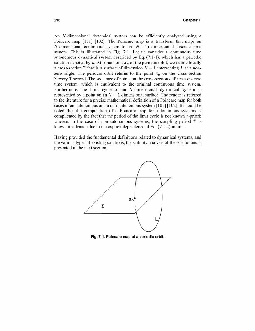
216
An -dimenPoincare ma
-dimensionsystem. Thisautonomous solution denoa cross-sectiozero angle. Σ every T sectime systemFurthermore,represented bto the literatucases of an aunoted that thcomplicated whereas in tknown in adv Having provithe various typresented in t
nsional dynamap [101] [102nal continuous is illustratedynamical sy
oted by . At on Σ that is aThe periodiccond. The seq, which is e, the limit by a point on ure for a preciutonomous anhe computatiby the fact ththe case of nvance due to t
ided the fundypes of existinthe next secti
Fig. 7-
mical system2]. The Poinus system to ed in Fig. 7ystem describsome point
a surface of dc orbit returnquence of poinequivalent tocycle of anan 1 dim
ise mathematind a non-autoion of a Poihat the periodnon-autonomthe explicit de
damental definng solutions, on.
-1. Poincare m
m can be efncare map is
an ( 1) -1. Let us cbed by Eq. (7
of the periodimension ns to the points on the cro
o the originan -dimensiomensional surical definitiononomous systincare map fd of the limit
mous systems,ependence of
nitions relatedthe stability a
map of a period
fficiently anaa transformdimensional
consider a co7.1-1), which odic orbit, we1 intersecti
int on theoss-section deal continuousonal dynamirface. The rean of a Poincarem [101] [10for autonomocycle is not k, the samplinf Eq. (7.1-2) in
d to dynamicaanalysis of th
dic orbit.
Chapter
alyzed using m that maps
l discrete timontinuous timhas a period
e define localing at a noe cross-sectio
efines a discres time systemical system ader is referrre map for bo
02]. It should bous systems known a-priong period n time.
al systems, anhese solutions
r 7
a an
me me dic lly
on-on ete m. is
red oth be is
ori; is
nd is
Perturbation Models 217
7.1.1 Introduction to Stability Analysis of Nonlinear Dynamical Systems
There exist different types of stability. For the precise mathematical definitions and types of stability, the reader is referred to the literature [94] [101]. For the purposes of this work, a rather qualitative definition is provided. A steady state
is (Lyapunov) stable if and only if there exists a neighborhood of such that every trajectory with initial condition ∈ remains within at all times 0. Furthermore, a steady state is asymptotically stable if and only if there exists a neighborhood of such that every trajectory with initial condition ∈ reaches arbitrarily close to given enough time 0. In other words, the -limit set of any initial condition within is . Conversely, a steady state is unstable if there exists a neighborhood of such that is the -limit set of all initial conditions in . Finally, a steady state is called non-stable if for every neighborhood , there exists at least one point whose
-limit set is and one point whose -limit set is .
7.1.2 Equilibrium Point
The stability of an equilibrium point is examined by considering the linear perturbation of the vector field at . The eigenvalues of the Jacobian
of the vector field determine the stability of the solution.
(7.1-6)
with representing an initial perturbation from .The solution of the linear differential equation Eq. (7.1-6) generally takes the form
(7.1-7)
where and are the eigenvalues and eigenvectors of , respectively. The constants are determined by the initial condition . For a given -dimensional vector field the Jacobian matrix has
eigenvalues. An equilibrium point whose eigenvalues do not have a real part equal to zero is called hyperbolic. If all eigenvalues have negative real parts, the point is asymptotically stable. Correspondingly, if there exists one eigenvalue with a positive real part, is unstable. Finally, if there exists one eigenvalue with a real part equal to zero, the equilibrium point is non-hyperbolic, a condition that is equivalent to the determinant of being equal to zero, and the eigenvalues of are not sufficient to determine its stability.
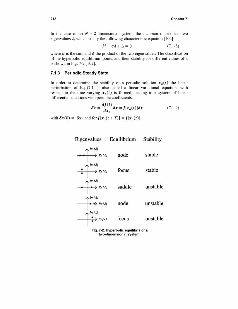
218
In the case eigenvalues
where is thof the hyperbis shown in F
7.1.3 Peri
In order to perturbation respect to thdifferential e
with 0
of an 2, which satis
he sum and Δ bolic equilibrFig. 7-2 [102]
odic Steady
determine thof Eq. (7.1-
he time varyiquations with
and fo
Fi
2-dimensionasfy the follow
the product oium points an.
y State
he stability o-1), also calling is
h periodic coe
or
g. 7-2. Hyperbtwo-dimens
al system, thewing character
Δ 0
of the two eignd their stabil
of a periodicled a linear
formed, leaefficients.
bolic equilibriasional system
e Jacobian mristic equation
genvalues. Thlity for differ
c solution variational
ding to a sy
.
a of a .
Chapter
matrix has twn [102]
(7.1-8)
he classificatiorent values of
the lineequation, wi
ystem of line
(7.1-9)
r 7
wo
on f
ear ith ear
Perturbation Models 219
The solution of Eq. (7.1-6) is derived using Floquet theory [94]
(7.1-10)
where are the Floquet multipliers and are periodic vector functions. The Floquet exponents are related to the multipliers by
(7.1-11)
It is seen from Eq. (7.1-11) that there is not a unique mapping between multipliers and exponents, as adding to any exponent a complex factor 2 ⁄ with an arbitrary integer results in the same multiplier. The stability of is determined by the Floquet multipliers . They can be calculated by direct integration of Eq. (7.1-9) for one period with initial condition 0 where is the identity diagonal square matrix of dimension . The result of the integration is the monodromy matrix whose eigenvalues are the desired Floquet mutlipliers [94]. A periodic solution of an autonomous system has at least one Floquet multiplier with magnitude equal to 1, or equivalently a Floquet exponent equal to zero. Furthermore, a periodic solution is stable if the remaining multipliers have a magnitude less than one (| |<1). Correspondingly, if one multiplier with magnitude larger than 1 exists, the solution is unstable.
7.1.4 Lyapunov Exponents
The Lyapunov exponents are defined as follows
lim→
1ln (7.1-12)
and can be considered a generalization of both the characteristic eigenvalues of the equilibrium point and the Floquet multipliers of the periodic steady state [101]. In fact, the Lyapunov exponents can be used to determine the stability of quasi-periodic and chaotic steady-state solutions. One can easily see from Eq. (7.1-7) that the Lyapunov exponents of the equilibrium point correspond to the real part of the characteristic eigenvalues.
, (7.1-13)
Correspondingly the Lyapunov exponents of the periodic steady state are equal to the natural logarithm of the magnitude of the Floquet multipliers divided by
220 Chapter 7
the period of the solution which is equal to the real part of the Floquet exponents.
,ln| |
(7.1-14)
7.2 Bifurcations of Nonlinear Dynamical Systems
A dynamical system described by Eq. (7.1-1), in practice depends on a set of parameters of dimension ( ∈ ) which enter the definition of the vector field
, (7.2-1)
A parameter corresponds to some circuit control voltage or bias voltage/current or any other physical parameter such as the dimension of a transmission line. As the parameter vector varies, the solutions of Eq. (7.2-1) change. The change of stability of a specific steady-state solution, the creation of new steady-state solutions or elimination of existing ones, as one or more parameters of a nonlinear system vary is called a bifurcation [100,102]. The corresponding parameter values for which a bifurcation occurs are called bifurcation values. A bifurcation diagram is a plot of a selected state variable(s) corresponding to a limit set versus the system parameter(s). An example of a bifurcation diagram is the plot of the DC voltage at a selected circuit node or the oscillation amplitude versus the external bias voltage of the oscillator. Bifurcations are classified into local and global. Local bifurcations are detected by studying the vector field f in a neighborhood of a limit set. In contrast, local information is not sufficient to detect global bifurcations. Typically in this book we study systems where one parameter is varied ( 1).
7.2.1 Bifurcations of Equilibrium Points
Let us consider such a continuous time system with one parameter that has a hyperbolic equilibrium point. As the parameter varies, there are two ways that a hyperbolic point can become non-hyperbolic. In the first one, a simple real eigenvalue becomes zero ( 0). In this case the system is going through a bifurcation known as fold bifurcation. Fold bifurcation is also known as turning-point or saddle-node bifurcation. In a fold bifurcation the equilibrium point curve presents an infinite slope at the parameter value where one real eigenvalue becomes zero. This is seen in the bifurcation diagram of a one-dimensional system shown in Fig. 7-3.
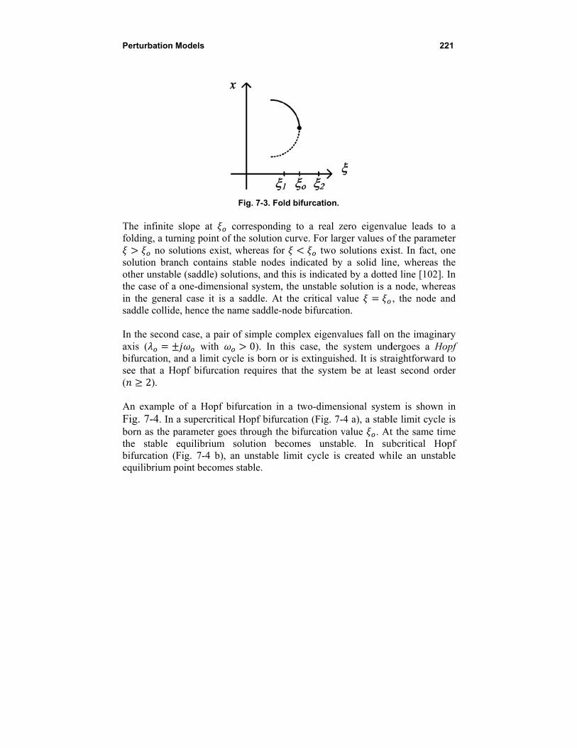
Perturbation M
The infinite folding, a tur
no sosolution branother unstablthe case of ain the generasaddle collide In the secondaxis (bifurcation, asee that a H( 2). An example Fig. 7-4. In born as the pthe stable bifurcation (equilibrium p
Models
slope at rning point ofolutions exist,nch contains le (saddle) soa one-dimensial case it is e, hence the n
d case, a pair with
and a limit cyopf bifurcatio
of a Hopf ba supercritica
parameter goeequilibrium Fig. 7-4 b), point become
Fig. 7-3. Fol
correspondinf the solution , whereas forstable nodes
lutions, and tional system,a saddle. At
name saddle-n
of simple co0). In th
ycle is born oon requires t
bifurcation inal Hopf bifurces through thsolution be
an unstable ls stable.
ld bifurcation.
ng to a real curve. For la
r two s indicated bythis is indicatethe unstable the critical v
node bifurcati
omplex eigenvhis case, the
or is extinguisthat the syste
n a two-dimencation (Fig. 7e bifurcation
ecomes unstalimit cycle is
.
zero eigenvaarger values o
solutions exiy a solid lined by a dottesolution is a
value ion.
values fall on system und
shed. It is straem be at leas
nsional syste7-4 a), a stabl
value . Atable. In subs created wh
22
alue leads tof the parametist. In fact, on
ne, whereas thed line [102]. a node, where, the node an
n the imaginadergoes a Hoaightforward st second ord
em is shown le limit cycle t the same timbcritical Ho
hile an unstab
21
a ter ne
the In
eas nd
ary opf
to der
in is
me opf ble
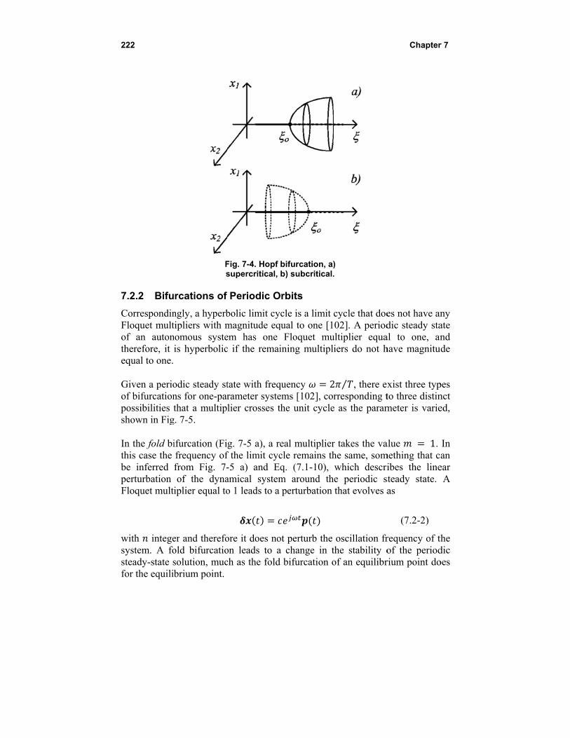
222
7.2.2 Bifu
CorrespondinFloquet multof an autontherefore, it equal to one. Given a perioof bifurcationpossibilities tshown in Fig In the fold bithis case the be inferred perturbation Floquet mult
with integesystem. A fosteady-state sfor the equili
Fs
rcations of
ngly, a hyperbtipliers with mnomous systeis hyperbolic
odic steady stns for one-parthat a multip
g. 7-5.
ifurcation (Fifrequency offrom Fig. 7-of the dyna
iplier equal to
er and therefoold bifurcatiosolution, mucbrium point.
Fig. 7-4. Hopf supercritical,
Periodic O
bolic limit cymagnitude eqem has one c if the remai
tate with freqrameter systelier crosses t
g. 7-5 a), a ref the limit cyc-5 a) and Eqamical systemo 1 leads to a
ore it does noon leads to ach as the fold
bifurcation, a)b) subcritical.
rbits
cle is a limit qual to one [1
Floquet muining multipl
quency 2ems [102], corhe unit cycle
eal multipliercle remains thq. (7.1-10), m around thperturbation
ot perturb the a change in t
bifurcation o
) .
cycle that doe02]. A period
ultiplier equaiers do not h
2 ⁄ , there exrresponding t
e as the param
r takes the vahe same, somwhich descrie periodic sthat evolves a
oscillation frthe stability oof an equilibr
Chapter
es not have andic steady staal to one, anhave magnitu
xist three typto three distinmeter is varie
alue 1. mething that c
ibes the linesteady state. as
(7.2-2)
requency of tof the periodrium point do
r 7
ny ate nd
ude
pes nct ed,
In an
ear A
the dic oes
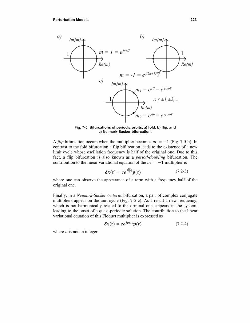
Perturbation M
F
A flip bifurcacontrast to thlimit cycle wfact, a flip bcontribution
where one caoriginal one. Finally, in a multipliers apwhich is notleading to thvariational eq
where is no
Models
Fig. 7-5. Bifurcc
ation occurs whe fold bifurcawhose oscillatbifurcation isto the linear v
an observe th
Neimark-Sacppear on the t harmonicalle onset of a qquation of thi
ot an integer.
cations of peric) Neimark-Sa
when the mulation a flip bition frequencs also knownvariational eq
he appearance
cker or torusunit cycle (Fy related to quasi-periodics Floquet mu
odic orbits, a)cker bifurcatio
ltiplier becomifurcation leay is half of th
n as a periodquation of the
e of a term w
bifurcation, aFig. 7-5 c). Athe orininal oc solution. Th
ultiplier is exp
) fold, b) flip, aon.
mes 1ads to the exishe original od-doubling bi 1 mu
with a frequen
a pair of comAs a result a none, appears he contributio
pressed as
22
and
(Fig. 7-5 b). stence of a nene. Due to thifurcation. T
ultiplier is
(7.2-3)
ncy half of t
mplex conjuganew frequencin the system
on to the line
(7.2-4)
23
In ew his he
the
ate cy, m, ear
224 Chapter 7
7.3 The Averaging Method and Multiple Time Scales
The averaging method is typically used to analyze the periodic steady-state solutions of weakly nonlinear systems
, (7.3-1)
and perturbations of the linear oscillator systems [103] [100], with ≪ 1. It was originally developed by Krylov and Bogoliubov [104]. The
method is particularly suitable to analyze the perturbed linear oscillator problem described by
ω (7.3-2)
where , , ∈ . The van der Pol differential equation belongs to this class of systems with 1 . In the case of weakly coupled oscillators, an equation of the form Eq. (7.3-2) is used to describe each oscillator, and contains the nonlinear term of the free-running (uncoupled) oscillator as well as contributions from external coupled signals from other oscillators, which can be linear or nonlinear. The averaging theorem [100] Uc585947 states that there exists a change of coordinates , which transforms Eq. (7.3-1) to the averaged system
(7.3-3)
where
12
,0 (7.3-4)
The system given by Eq. (7.3-3) is an autonomous system, whereas Eq. (7.3-1) can be non-autonomous. The essential property of the averaged system that is extensively applied in the study of coupled oscillator systems is that a hyperbolic periodic steady state of Eq. (7.3-3) corresponds to a hyperbolic equilibrium point of Eq. (7.3-1) and that both steady states have the same stability [100]. This essentially means that the eigenvalues of the linearized system of an equilibrium point of Eq. (7.3-3) determine its stability. This is quite useful as obtaining the Floquet multipliers of a microwave oscillator may not be a trivial task. Furthermore, for the cases that are considered in this book, the bifurcations of the averaged system are the same as those of the original system [100]. In order to transform the perturbed linear oscillator problem in the standard form Eq. (7.3-1), the following transformation (known as the van der Pol transformation [100] [103]) is commonly applied to Eq. (7.3-2) before averaging,
Perturbation Models 225
(7.3-5)
In this case Eq. (7.3-2) becomes
, , , , (7.3-6)
, , , ,
Applying Eq. (7.3-4), the averaged solution is obtained
, (7.3-7)
,
It should be noted that the transformation given by Eq. (7.3-5) and subsequent application of the perturbation method limits the analysis of the system given by Eq. (7.3-2) locally near the oscillation frequency in the frequency domain. The system can be studied near a different harmonic by modifying appropriately the transformation, that is, setting in place of where is the desired harmonic order. In practice, considering the oscillator behavior near the fundamental frequency is sufficient for the study of high Q oscillators because higher harmonics are small and therefore can be ignored in the analysis. Specifically, the averaged Van del Pol differential equation for which
1 becomes [103]
2
1
4 (7.3-8)
0
The above system leads to a nontrivial steady-state oscillation with amplitude 2 obtained by requiring that 0.
7.4 Averaging Theory in Coupled Oscillator Systems
Kurokawa considered the oscillator equivalent of a series resistance, inductance, capacitance (RLC) resonator connected in series with a negative resistance and applied the averaging theory to study the properties of noisy oscillators and injection locked oscillators [105].
226 Chapter 7
The theory of Kurokawa applied to the study of coupled oscillator arrays was introduced to the antennas and microwaves communities by Stephan [1] with an aim towards antenna-array applications such as power-combining arrays and phased arrays. The work of Stephan focused on taking advantage of the dynamical properties of coupled oscillator array topologies in order to generate constant phase shift distributions among the array elements in a continuously variable manner. A parallel RLC resonator in parallel with a negative resistance was used to model each oscillator, leading to a dual form of the one used by Kurokawa. It should be noted that there is significant theoretical work in the literature regarding coupled oscillator systems, also called distributed and ladder oscillators, considering the various operating modes and stability of one- and two-dimensional arrays. Notable references are [106] [107] [108] [109]. The latter work by Endo and Mori [109] presented an elegant way to obtain a formulation equivalent to a perturbed van der Pol equation in vector form for an array of coupled oscillators modeled as a parallel RLC resonator with a negative resistance, and it will be given in the next section. An efficient analysis of coupled oscillator arrays for quasi-optical power combining and the stability of the various existing operating modes was proposed by York and Compton [110] utilizing only the phase dynamics of the array, or in other words the second equation of Eq. (7.3-7). We may distinguish among power-combining applications where the stability of the various operating modes of coupled oscillator systems is with an aim to secure excitation of only the in-phase mode, and applications where an arbitrary phase distribution among the oscillator elements is required (such as beamforming and phased arrays). The latter may be viewed as a generalization of the former. Following their initial work, York produced a general formulation for coupled-oscillator arrays based on the fundamental harmonic approximation and the averaging method that is essentially used to date in most approximate analysis methods for such systems [111], [95]. Furthermore, York introduced an elegant way to achieve constant progressive phase shifts among the array oscillator elements in a continuous fashion by only modifying the oscillation frequency of the end elements of the array. In 2004, Heath presented an elegant and unifying formulation of the application of the method of averaging (specifically the Lindstedt method was used to derive the slow time differential equations [94]) in coupled-oscillator arrays along with a detailed stability analysis of various different coupling network topologies [112]. The latter formulation is given here

Perturbation Models 227
cos Φ (7.4-1)
Δ
Φ
where an array of oscillators is assumed. The variable represents the slowly varying averaged amplitude of oscillator , as given in Eq. (7.3-7) with the bar suppressed for simplicity. Correspondingly, the phase of oscillator is given by where is the averaged time varying component of the oscillator phase corresponding to Eq. (7.3-7) (with the bar suppressed). When uncoupled to the rest of the array elements, each oscillator has a periodic steady state with amplitude and frequency Δ . Furthermore, each individual oscillator satisfies a van der Pol differential equation of nonlinearity constant , which appears in Eq. (7.4-1) through
2⁄ where is the external quality factor of the resonator of each oscillator element calculated using a reference load admittance . Coupling among the oscillator elements is included in the form of a square complex matrix of dimension , with . Note that is a transfer function (unitless). If for example an admittance matrix is used to express the coupling among oscillator elements, then is the admittance matrix normalized to the reference load admittance . In Eq. (7.4-1) the coupling coefficients also appear in normalized form setting
/2 (7.4-2)
Finally, Eq. (7.4-1) can be written in a complex valued compact format letting
Δ | | (7.4-3)
Under weak coupling conditions, the phase dynamics alone are sufficient to analyze the behavior of the coupled oscillator system. We may then consider only the second equation of Eq. (7.4-1) and assume that the oscillator amplitudes are approximately equal to their uncoupled values . The system of equations pertaining to the phase dynamics provide significant insight and a very computationally efficient method to analyze arrays with a
228 Chapter 7
large number of elements. In fact, the analysis results of Part I of this book have focused on the phase dynamics of coupled oscillator arrays. The system of equations limited to the phase dynamics was introduced as the “generalized phase model” by Heath in [112]:
Δ Φ (7.4-4)
When no coupling phase Φ is considered, the model is the well known Kuramoto model [113]. In the special case where a bi-directional symmetrical coupling matrix with = is considered, the generalized phase model coincides with the phase model introduced by York in [111]. A fixed point of Eq. (7.4-1) corresponds to a periodic steady-state solution, defined for 0 and with an arbitrary constant. Letting take nonzero values still corresponds to synchronized solutions of the array but for a different frequency than .
cos Φ
0
(7.4-5)
Δ Φ
0
Every set , that satisfies the above conditions corresponds to an oscillating mode of the array. In principle there exist up to 2 modes [111]. It should be emphasized that, due to the autonomous nature of the coupled oscillator system, it is possible to translate all oscillator phases by the same arbitrarily large value and still obtain the same steady-state solution. This is evidenced by the fact that only phase differences appear in Eq. (7.4-5). In other words, the steady state is defined by the oscillator phase differences and not their absolute phase. The stability of the oscillating modes is examined by considering the linear perturbation , of Eq. (7.4-1), which leads to a system of linear differential equations
Perturbation Models 229
3
Φ
Φ
(7.4-6)
Φ
Φ
In the case of the generalized phase model one has
Φ (7.4-7)
Because the steady state is defined by phase differences and not absolute phase values, the perturbation phase values of the steady state may not be small. Their differences, however, are assumed to be small, and this allows one to take the linear approximation of the cosine and sine terms in Eq. (7.4-1) and obtain Eq. (7.4-6).
7.5 Obtaining the Parameters of the van der Pol Oscillator Model
A useful analytical method is presented, that allows one to obtain the van der Pol differential equation from a parallel resonator with a nonlinear voltage dependent current source. The procedure follows the development presented by Endo and Mori in [108], and it represents a time-domain formulation of van der Pol’s model described in Section 1.2. This model has very low complexity, and it can be easily incorporated into analysis of large arrays or proof of concept for various topologies of coupled oscillators. In addition, it can be easily introduced into circuit simulators.
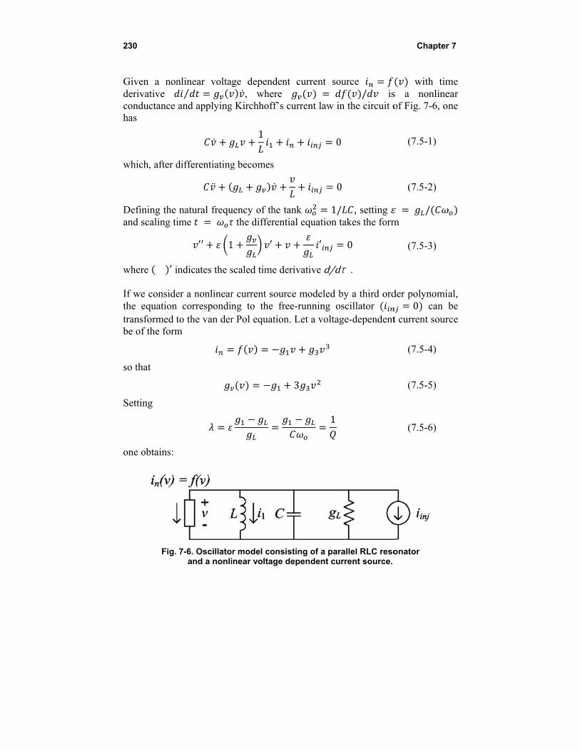
230
Given a nonderivative conductance has
which, after d
Defining the and scaling ti
where ′ i If we considethe equationtransformed tbe of the form
so that
Setting
one obtains:
Fig.
nlinear volta⁄
and applying
differentiating
natural frequime
′′ 1
indicates the s
er a nonlinearn correspondito the van derm
7-6. Oscillatoand a nonli
age dependen, where
g Kirchhoff’s
1
g becomes
uency of the t the different
1 ′
scaled time de
r current sourng to the frr Pol equation
or model consinear voltage
nt current so
current law in
0
0
tank 1/tial equation t
′
erivatived/d
rce modeled bee-running on. Let a voltag
3
1
isting of a pardependent cu
ource / is
n the circuit o
0
0
/ , setting takes the form
0
dτ.
by a third ordoscillator ge-dependent
rallel RLC resourrent source.
Chapter
with tims a nonlineof Fig. 7-6, on
(7.5-1)
(7.5-2)
/m
(7.5-3)
der polynomia0 can b
t current sour
(7.5-4)
(7.5-5)
(7.5-6)
onator
r 7
me ear ne
al, be
rce
Perturbation Models 231
13
′ ′ 0 (7.5-7)
The parameter λ is equal to the inverse of the loaded quality factor, Q, of the oscillator circuit of Fig. 7-6. Finally, scaling the voltage as
3
(7.5-8)
the differential equation takes the desired form:
1 ′3
′ 0 (7.5-9)
When no injection signal is present, 0, and this equation becomes the well known van der Pol equation.
1 ′ 0 (7.5-10)
The approximate solution to the van der Pol oscillation is [94]
2 cos ⇒2sin (7.5-11)
which is identical to the solution provided by the averaging method in Section 7.3. The approximate parallel model for the oscillator can be extracted using a nonlinear simulator and calculating the admittance at a selected circuit node [114]. Several authors have proposed experimental techniques to evaluate the model parameters [114,115]. Measurement of the oscillator amplitude can be used to obtain the scaling parameter . Injection locking the oscillator to an external signal and measuring the locking bandwidth can be used to estimate the Q and subsequently the second parameter of the van der Pol model [114]. Alternatively, a low-frequency sinusoidal modulating signal can be introduced in the bias circuitry of the oscillator, resulting in a phase modulated oscillator output. The parameter can then be obtained by measuring the relative amplitude of the modulation sidebands [115].
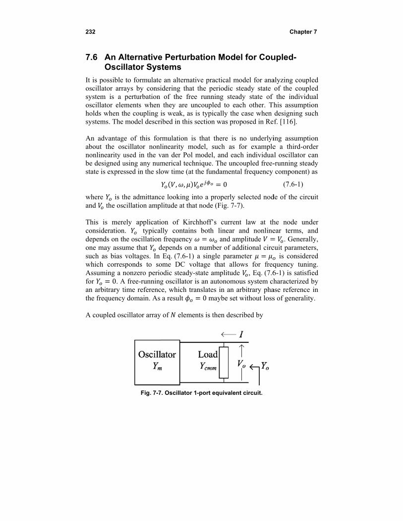
232
7.6 An AOsci
It is possibleoscillator arrsystem is a oscillator eleholds when tsystems. The An advantagabout the osnonlinearity be designed ustate is expre
where is tand the os This is merconsiderationdepends on thone may assusuch as bias which corresAssuming a nfor 0. Aan arbitrary tthe frequency A coupled os
Alternativellator Sys
e to formulaterays by consiperturbation
ements when the coupling e model descri
ge of this forscillator nonlused in the vusing any num
essed in the sl
the admittanccillation amp
rely applicatin. typicahe oscillationume that dvoltages. In
sponds to sononzero perio
A free-runningtime referency domain. As
scillator array
Fig. 7-7
e Perturbastems
e an alternatividering that t
of the free they are unc
is weak, as isibed in this se
rmulation is linearity modvan der Pol mmerical technow time (at th
, ,
ce looking intplitude at that
ion of Kirchlly contains
n frequency depends on a
Eq. (7.6-1) aome DC volodic steady-stg oscillator is
ce, which trana result
y of elemen
7. Oscillator 1-
ation Mod
ve practical mthe periodic running stea
coupled to es typically thection was pr
that there isdel, such as
model, and eanique. The unhe fundament
0
to a properly node (Fig. 7-
hhoff’s currenboth linear
and amnumber of ad
a single paramtage that alltate amplituds an autonomonslates in an 0 maybe set
nts is then des
-port equivale
el for Cou
model for anasteady state ady state of ach other. The case when oposed in Re
no underlyifor example
ach individuancoupled free-tal frequency
selected nod-7).
nt law at thand nonline
mplitude dditional circmeter lows for freqde , Eq. (7.6ous system charbitrary phat without loss
cribed by
nt circuit.
Chapter
upled-
alyzing couplof the couplthe individu
his assumptiodesigning suf. [116].
ing assumptioe a third-ordal oscillator c-running steadcomponent)
(7.6-1)
de of the circu
he node undear terms, an
. Generallcuit parameter
is considerquency tunin6-1) is satisfiharacterized b
ase reference s of generality
r 7
ed ed
ual on
uch
on der an dy as
uit
der nd ly, rs,
red ng. ed by in
y.
Perturbation Models 233
0 (7.6-2)
where the coupling is represented by the admittance matrix which typically is frequency dependent. The coupling results in a steady state that can be expressed as a perturbation of the individual oscillator free-running steady state as follows:
Δ (7.6-3)
Δ
Δ
, ,
The perturbation assumption has been used in the first place by York, Liao, and Lynch [33], and it is described in Section 1.3 dealing with the injection-locked oscillator. However, in their analysis they proceed to assume a specific nonlinear dependence of the adminttance on the amplitude whereas here no such assumption is made. Furthermore, it should be noted that the frequency expansion has been done using the well known Kurokawa transformation [105] introduced in Section 1.3. The commonly used coupling networks have a broadband frequency response relative to the oscillator locking bandwidth, which allows us to consider a constant coupling term . Narrowband coupling networks were studied by Lynch and York [117]. After some straightforward manipulation, one obtains
234 Chapter 7
Δ
0
(7.6-4)
This system of differential equations represents the basis for an alternative model formulation for a system of coupled oscillators. This formulation has been essentially introduced in Ref. [116] and refined in Ref. [118] as well as subsequent works as a basis to study several properties of coupled oscillator arrays. In order to appreciate the similarities and differences with the original model of Section 7.4, the amplitude and phase equations are decoupled by first dividing with ⁄ and then considering real and imaginary parts. Let for simplicity
(7.6-5)
| |
Using the above, Eq. (7.6-4) becomes
Δ
| | cos
0
(7.6-6)
Perturbation Models 235
Δ
| | sin
0
Furthermore, letting it is possible to express Eq. (7.6-6) in a compact complex form
| | Δ 0 (7.6-7)
The corresponding generalized phase model associated with this formulation is obtained considering only the phase dynamics which results in
Δ | | sin 0 (7.6-8)
The periodic steady-state solution is obtained by setting 0 and ∆ leading to
Δ
| | cos
0
(7.6-9)
∆ Δ
| | sin
0
or in complex notation
∆ Δ
0 (7.6-10)
236 Chapter 7
As was the case with the model represented by Eq. (7.4-1) the steady state of the array is defined by phase differences and not absolute phases. In order to study the stability of the steady-state solution, we form the linear perturbation of Eq. (7.6-4) using , , where small-amplitude perturbations and small-phase perturbation differences are considered leading to
2
| | cos
| | sin
0
(7.6-11)
∆ 2
| | sin
| | cos
0
Correspondingly, the generalized phase model stability is then determined by
| | cos 0 (7.6-12)
The eigenvalues of the linear variational equation determine the stability of the steady-state solutions. In practice, it is more computationally efficient to formulate and process the array equations as matrix equations, and this is the topic of the next section.
7.7 Matrix Equations for the Steady State and Stability Analysis
It is easier from a computational point of view to express the various systems of equations of the previous sections in matrix form. In order to do so, the
Perturbation Models 237
following notation and properties are used. Bold letterface indicates a column vector or a matrix. The dimension of the vector or square matrix is unless noted otherwise, 0 and indicate a vector of zeros and a vector of ones, respectively. The notation and define a vector and a matrix , respectively. The function dg converts a vector to a square diagonal matrix of size . It is straightforward to show that for any two vectors and , dg dg . The superscript indicates the conjugate transpose of a matrix or vector, whereas superscripts and indicate real and imaginary part. One can then rewrite Eq. (7.4-1) in matrix form
dg dg (7.7-1)
where dg . The system given by Eq. (7.7-1) can be integrated numerically after separating real and imaginary parts,
dgdg
dg (7.7-2)
where the vector function is defined as . The generalized phase model (7.4-4) is then given by
(7.7-3)
The steady state of Eq. (7.7-2) is computed by setting 0 and which, when substituted in (7.7-2), result in the trivial solution or
dg
dg (7.7-4)
The linear variational equation of Eq. (7.7-1) is also written as a matrix linear differential equation as follows
dg (7.7-5)
with
dg (7.7-6)
dg dg
where 3 . The complex system of Eq. (7.7-5) is separated into real and imaginary parts as
dg (7.7-7)
238 Chapter 7
or
dg dg
(7.7-8)
where dg is a diagonal matrix with the inverse of the steady-state oscillator amplitudes in its diagonal. The inversion operation is guaranteed to exist under the assumption that the steady-state solution corresponds to nonzero amplitudes for all oscillators. Correspondingly, the linear variational equation of the generalized phase model is
(7.7-9)
The matrix differential equation pertaining to the coupled-oscillator dynamics according to the alternative model Eq. (7.6-4) becomes
dg dg ∆ (7.7-10)
where dg . After separating into real and imaginary parts one obtains
dg
dg ∆
dg ∆
(7.7-11)
The steady-state solution is then given by the nonlinear system of algebraic equations
dg ∆
dg ∆ dg ∆
(7.7-12)
Due to the perturbation assumption, one may consider a linear approximation of the steady state as follows
Perturbation Models 239
1
1∆∆ ∆
(7.7-13)
For a given frequency offset ∆ and phase distribution along the array elements contained in Φ, one may solve the above linear system of 2 equations for the
steady-state oscillator amplitudes and control perturbations. Alternatively, one may fix the control parameter of one arbitrarily selected oscillator and solve the steady-state system for the steady-state oscillator amplitudes, 1 remaining control perturbations and frequency offset ∆ . The stability of the steady-state solution is obtained taking the linear variational equation of Eq. (7.7-10) leading to the following linearized system of differential equations
dg (7.7-14)
where
∆ dg ∆ (7.7-15)
dg dg
where 2 . One then separates real from imaginary parts to obtain the desired system of linear differential equations
dg (7.7-16)
or
dg dg
(7.7-17)
The 2 eigenvalues of the square matrix determine the stability of the solution. It should be noted that due to the autonomous nature of the coupled-oscillator array one eigenvalue of is always zero. The solution is stable if all remaining eigenvalues of have negative real parts. One can easily verify that is unchanged to phase shifts that are common to all oscillators. This is due to the fact that matrix contains only
240 Chapter 7
phase differences between the various elements. It is then possible to reduce the system by one, thus eliminating the zero eigenvalue. Selecting an arbitrary element (for example, element ) as a reference, the phase equations of Eq. (7.7-17) can be reduced by one by subtracting row , the equation which corresponds to the phase of oscillator , from every other equation. The equation that corresponds to the phase of oscillator can then be eliminated. Furthermore, the elements of column from row 1 to 2 are multiplied by zero. In addition, in the amplitude equations, due to the fact that
contains only phase differences, it is possible to subtract from all
phases forming ← . As a result column can also be eliminated because it is being multiplied by zero. The remaining square matrix of dimension 1 has the same eigenvalues with minus the zero eigenvalue. Matrix corresponds to the system of 2 1 linear differential equations
(7.7-18)
where the vector of dimension 1 contains phase difference terms relative to oscillator . The spectral abscissa of a square matrix is the maximum real part of its eigenvalues [119]. Therefore a steady-state solution is stable if the spectral abscissa of is negative.
7.8 A Comparison between the Two Perturbation Models for Coupled Oscillator Systems
The similarity of the two models is made obvious by comparing the two expressions corresponding to the generalized phase model Eq. (7.4-4) and Eq. (7.6-8). The first model is defined for a parallel RLC tank with a nonlinear voltage-dependent current source that exhibits a third-order nonlinearity similar to the one described in Section 7.5 and shown in Fig. 7-6. In this case, the admittance looking at the output node of the circuit is given by
,1
(7.8-1)
where contains the nonlinear admittance of the current source at the fundamental frequency component. The total admittance contains a real nonlinear admittance term that is amplitude dependent, plus the load admittance, and an imaginary term which is frequency dependent. As a result, a real derivative versus the amplitude and an imaginary admittance derivative versus the frequency are obtained:
Perturbation Models 241
(7.8-2)
2
Furthermore, if we consider that for a parallel resonant circuit the external quality factor is given by
(7.8-3)
it is straightforward to verify that the Eqs. (7.4-4) and (7.6-8) are identical. In general, active devices in microwave frequencies exhibit nonlinear susceptance as well as admittance, in addition to a nonlinear admittance that is frequency dependent. In other words a more general expression for the admittance at an oscillator circuit node is
, , , (7.8-4)
As a result, it is possible to view the alternative model (7.6-4) using complex admittance derivatives as a generalized version of (7.4-1).
7.9 Externally Injection-Locked COAs
The coupled-oscillator array is an autonomous system that behaves like a single distributed oscillator. However, there are several applications that require the array to be injection-locked to an external signal. The reason can be to control the phase distribution among the array elements [1], to reduce the array phase noise [97], to fix the array frequency [120], or to introduce modulation to the array [121] [122]. An external injection signal introduces an additive forcing term in the time-domain expression of the perturbed oscillator equation. In Section 7.5, it was demonstrated that the topology of a parallel RLC tank with a nonlinear voltage-dependent current source and an external-injection current term leads to the forced van der Pol equation. The coupled-oscillator system of differential equations is derived by applying Kirchhoff’s current or voltage law at a selected circuit node or loop of each oscillator circuit in the array. Specifically, in the parallel-tank topology, the corresponding equations are obtained by applying Kirchhoff’s current law at the output nodes of each oscillator. In addition, these nodes correspond to the nodes where the coupling network is connected to each oscillator. However,
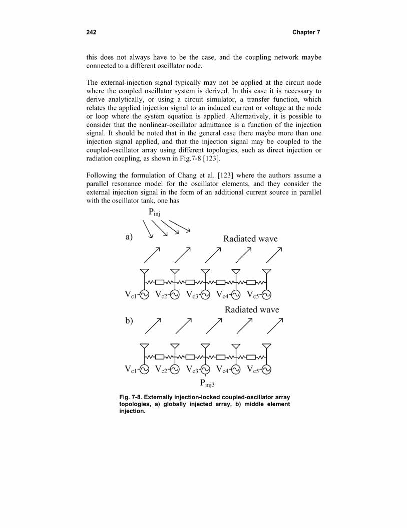
242
this does noconnected to The externalwhere the coderive analyrelates the apor loop wherconsider thatsignal. It shoinjection signcoupled-oscilradiation cou Following thparallel resoexternal injecwith the oscil
Fitoin
t always hava different os
-injection sigoupled oscillaytically, or uspplied injectiore the systemt the nonlineaould be notednal applied, llator array u
upling, as show
he formulationnance modelction signal illator tank, on
ig. 7-8. Externopologies, a) njection.
ve to be the scillator node
gnal typicallyator system issing a circuion signal to a
m equation isar-oscillator ad that in the gand that the
using differenwn in Fig.7-8
n of Chang el for the oscin the form one has
ally injection-globally injec
case, and the.
y may not be s derived. In it simulator, an induced cus applied. Altadmittance isgeneral case injection sig
nt topologies,8 [123].
et al. [123] wcillator elemef an addition
-locked couplected array, b
he coupling n
applied at ththis case it a transfer fu
urrent or voltaternatively, its a function othere maybe
gnal may be , such as dire
where the autents, and thenal current sou
ed-oscillator ab) middle elem
Chapter
network mayb
he circuit nois necessary
function, whiage at the not is possible of the injectiomore than ocoupled to th
ect injection
thors assumeey consider thurce in parall
array ment
r 7
ybe
de to ch de to on ne
the or
e a the lel

Perturbation Models 243
cos Φ
cos Φ
(7.9-1)
Δ sin Φ
sin Φ
where it is assumed that oscillator is being injected by an external source . The transfer function /2 consists of a
complex normalized term multiplied with a scaling factor /2 as is done for the coupling terms from the other oscillator elements in the array. For the case of an injection-current term in parallel with the oscillator tank
1. Furthermore, when a single oscillator is considered, Eq. (7.9-1) reduces to Adler’s equation. Alternatively, it is possible to assume that the nonlinear oscillator admittance
, , , at the node under consideration additionally depends on the
injection signal present at an arbitrary node of the oscillator circuit. Assuming a low amplitude-injection signal relative to the oscillator amplitude ⁄ ≪ 1, a Taylor expansion of the oscillator admittance around the free running steady state gives, to first order, [124]
, , , , , , (7.9-2)
with
, cos
sin (7.9-3)
The first term , , is the one considered in Eq. (7.6-3), where no external injection signal is present. The second term , is a linear perturbation term due to the external injection signal, which depends on the relative phase between the oscillator and the injection signal. The admittance expression is then introduced in the model presented in Section 7.6 and repeated here for convenience
244 Chapter 7
0 (7.9-4)
in order to derive the desired system of equations. As the injection power increases, additional terms in the Taylor expansion can be included in order to improve the accuracy of the approximation [124].
7.10 Phase Noise
Perturbation theory is applied in noise analysis of oscillators as typically noise is modeled as a stochastic forcing term in the oscillator differential equation. The stochastic nature of noise and the nonlinear nature of the oscillator circuits make noise analysis a challenging problem. Applying the averaging theory, Kurokawa [105] presented an elegant analysis of phase noise of free-running and externally injection locked oscillators. A fundamental assumption in his formulation is that noise, described by a time-domain stochastic process can be expanded in a Fourier series around the arbitrarily chosen fundamental frequency as
(7.10-1)
with a complex noise process. In the following it is assumed that is a zero-mean white Gaussian process, which results in
and being uncorrelated white zero-mean Gaussian processes as well [105]. Extending the work of Kurokawa, Chang et al. [97] studied phase noise in mutually injection-locked coupled-oscillator arrays. Application of the noise expansion and averaging allows us to include the effect of noise in the oscillator formulation Eq. (7.4-1) in terms of . In the following, the subscript 1 is dropped for simplicity.
cos Φ
2
(7.10-2)
Perturbation Models 245
Δ
Φ
2
The solution of Eq. (7.10-2) is found in the form of a perturbation , where , is the solution to the noise-free system
of Eq. (7.4-1), leading to a forced variational system, which is the same as was considered in the study of the stability of the steady state with the addition of a noise-forcing term. As before, small amplitude-noise perturbations and small phase-noise- perturbation differences result in the forced linear system of differential equations
3
Φ
Φ
2
(7.10-3)
Δ
Φ
Φ
2
Correspondingly, the alternative model in the presence of noise is modified by including an additive complex noise term in Eq. (7.6-4), which leads to forcing terms and in the left hand side of the first and second equations of Eq. (7.6-11), respectively. For compactness, the formulation is not repeated here.
246 Chapter 7
Following Chang [97], we proceed to solve Eq. (7.10-3) by first applying a Fourier transform
Ω 3
Φ
Φ
2
(7.10-4)
Ω Δ
Φ
Φ
2
The frequency indicates offset from the fundamental , and the hat indicates a Fourier transformed variable. The linear system of Eq. (7.10-4) is processed easier in matrix form. Using the formulation of Section 7.7, it is possible to write Eq. (7.10-4) in the form
Ω (7.10-5)
or
(7.10-6)
with Ω where the noise terms have been normalized as and for compactness. It should be
clarified that the identity matrix in Eq. (7.10-5) is of dimension 2 . Correspondingly, the formulation pertaining to the generalized phase model is
Ω (7.10-7)
Perturbation Models 247
or
(7.10-8)
with Ω . The noise correlation matrix (Ω) of the oscillator array is given by
Ω ⟨ ⟩ (7.10-9)
where the superscript ()H denotes the conjugate transpose operation. The various noise contributions AM-AM AM-PM, PM-AM, and PM-PM are easily identified.1 The operator ⟨ ⟩ denotes ensemble average, and following [97], for white Gaussian processes one has
⟨ ⟩ ⟨ ⟩2
(7.10-10)
⟨ ⟩ ⟨ ⟩
with as the noise variance. Identical oscillators have been assumed and identical noise sources have been applied at each oscillator for simplicity. The spectral density of the oscillator array is given by the diagonal of (Ω). The noise correlation matrix is then given by
Ω2
(7.10-11)
The generalized phase model expression can be used to obtain an approximate, more simplified, expression for the correlation matrix Ω , without considering amplitude noise:
Ω2
(7.10-12)
Note that Ω is a square matrix of dimension containing all correlation terms among the noise quantities of the individual oscillators. The phase noise spectra Ω of the individual oscillators in the array are given by the diagonal elements of Ω , or
Ω2
dg (7.10-13)
1 AM is amplitude modulation, and PM is phase modulation.

248 Chapter 7
The phase noise spectrum Ω of a single oscillator element uncoupled to the rest of the array corresponds to , and is given by
Ω2
1Ω
(7.10-14)
This expression is in agreement with the one given by Kurokawa in Ref. [105] and demonstrates the dependence of Ω of the phase-noise spectrum for the case of white Gaussian noise sources. The expression for the phase noise spectrum vector Ω of each oscillator element in the array finally can be written
Ω Ω Ω dg (7.10-15)
In addition to the phase noise of the individual coupled oscillator elements , in quasi optical power combining applications, one is also interested in
the phase noise of the combined output of the oscillators . Assuming small perturbations, one may write the combined far-field amplitude as [97]
cos
cos
(7.10-16)
with
1 1
(7.10-17)
The phase noise spectrum Ω of the combined output is given by
Ω ⟨ ⟩1⟨ ⟩ (7.10-18)
which, with the help of Eq. (7.10-15) becomes
ΩΩ Ω
(7.10-19)
Evaluation of the individual oscillator phase noise and the combined output phase noise is generally possible only by numerically evaluating Eqs. (7.10-15) and (7.10-19) respectively. Nonetheless, Chang et. al. [97] were able to analytically study several cases commonly found in the literature.
Perturbation Models 249
One of the results obtained by Chang, et al. [97] corresponds to the case where dg , repeated here for convenience, is a
symmetric matrix . As one can see, depends both on the coupling network through , and on the steady-state phase distribution of the various oscillator array elements, through . It can be easily verified that
, which reflects the fact that the steady state is unchanged to within a common constant phase term added to all oscillator elements, or in other words, the fact that the steady state is defined by the phase differences of the various elements. Using the above two properties, Chang et al. [97] have shown by analytically evaluating that Ω , which results in
ΩΩ
(7.10-20)
This is an important result indicating that the phase noise of the combined array output is reduced by a factor compared to the individual free-running oscillator phase noise (as indicated in Section 6.4). It remains to identify under which conditions is symmetric. One characteristic example is when an in-phase steady-state solution is assumed ( and a reciprocal coupling network matrix with zero coupling phase . In the case of a reciprocal coupling network of near-neighbor bilateral coupling with zero coupling phase, is symmetric for any constant phase distribution among the oscillator elements. It was also shown that in this case the individual oscillator phase noise is also reduced by a factor when the oscillators are in-phase. The oscillator phase noise for steady states with phase distributions with non-zero progressive phase Δ degrades with increasing Δ up to the point where the array loses stability and the phase noise becomes equal to the free-running oscillator phase-noise value. Finally, it was shown by Chang et al. [97] that there is no phase noise improvement in the case of unilaterally coupled oscillators, both for the individual elements and the combined-array output (as indicated in Section 6.4). The phase noise of externally injection-locked oscillators has been investigated by Kurokawa in [105], where it was shown that the injected oscillator phase-noise spectrum follows the phase-noise profile of the injection-locking signal for small frequency offsets near the carrier, and it converges to the free-running oscillator phase-noise spectrum for large frequency offsets. The formulation of Kurokawa [105] was extended to externally injection locked coupled oscillator arrays by Chang, et al. [123]. It is straightforward to obtain the formulation pertaining to the externally injection-locked coupled-oscillator arrays by
250 Chapter 7
properly including in Eq. (7.10-2) terms due to injection sources as shown in (7.9-1). Chang et al. [123] investigated several topologies including a globally injected linear array, and arrays where a different single elements within the array are injected. In summary, the results showed that for small offsets the array phase-noise profile follows the injection-locking source phase-noise profile. However, for large offsets from the carrier the globally illuminated case showed a different behavior than the single-element illumination topology. In the former, the phase noise improves with increasing number of array elements, whereas in the latter the phase noise degrades with increasing number of elements. Furthermore, the array phase-noise performance of the single-element injection case improves as one injects an element closer to the array center.
7.11 Modulation
Several authors have considered the use of coupled-oscillator arrays in communication system applications. It is possible to distinguish among architectures where the coupled-oscillator array signal is modulated or architectures employing a coupled-oscillator array as the local oscillator in a multi-antenna up-converting or down-converting transceiver. The first topology has been studied by Kykkotis et. al. in [99]. Due to the limiting properties of oscillators, modulation formats that lead to large variations in the signal envelope are not recommended as the oscillator dynamics will tend to smooth these variations and introduce distortion. However, constant envelope modulation formats (such as constant phase modulation (CPM) and Gaussian minimum shift keying (GMSK)) represent excellent candidates to be employed in such systems. In Ref. [99], the modulation is applied in the coupled-oscillator array through an external injection signal. Additionally, it is possible to introduce modulation through the frequency-tuning bias voltage of the individual oscillators, as was proposed by Pogorzelski in Ref. [63]. A formulation based on Eq. (7.9-3) where the effect of the external-injection signal is included in the oscillator admittance was used by Collado and Georgiadis [124] to analyze the performance of such systems as the modulation bandwidth increases. The effect of the modulation on the maximum stable progressive constant phase shift among the oscillator elements was investigated, and it was shown that the presence of modulation leads to a reduction of the maximum achievable scanning range. In Fig. 7-9, the effect of sinusoidal phase modulation in the maximum scanning range of a two-element coupled oscillator array is shown. The maximum stable phase difference between the first harmonics of the two oscillators is obtained using the aforementioned model (denoted by RoM in Fig. 7-9), in good agreement with measurements as well as simulation results obtained using a commercial envelope transient circuit simulator. (The principles of nonlinear-circuit
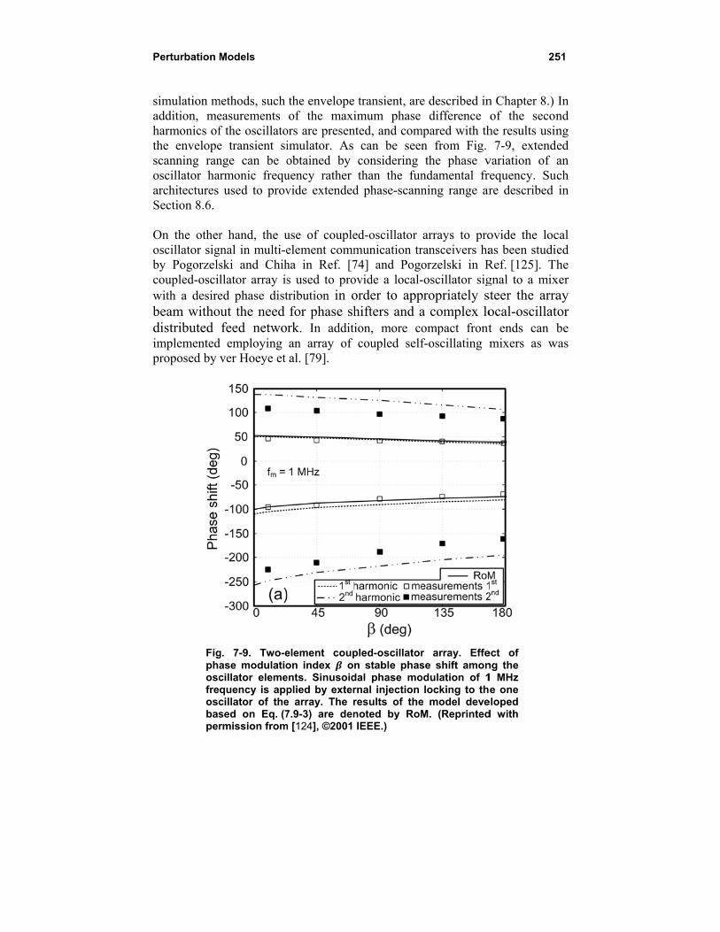
Perturbation M
simulation maddition, meharmonics ofthe envelopescanning ranoscillator haarchitectures Section 8.6. On the otheroscillator sigby Pogorzelscoupled-oscilwith a desirebeam withodistributed implementedproposed by
Figphaoscfreoscbasper
Models
methods, such easurements f the oscillatoe transient singe can be oarmonic frequ
used to prov
r hand, the ugnal in multi-eski and Chihllator array ised phase dist
out the need feed netwo
d employing ver Hoeye et
g. 7-9. Two-ease modulatiocillator elemequency is appcillator of thesed on Eq. (7rmission from
the envelopeof the maxi
ors are presenimulator. As obtained by uency rather vide extended
use of coupleelement commha in Ref. [7s used to protribution in ofor phase shrk. In additan array of al. [79].
element coupon index o
ents. Sinusoidplied by extere array. The r7.9-3) are den
m [124], ©2001
transient, areimum phase
nted, and comcan be seenconsidering than the fun
d phase-scann
ed-oscillator munication tr74] and Pogoovide a local-order to apphifters and aion, more cocoupled self
pled-oscillatorn stable phas
dal phase mornal injection results of thenoted by RoMIEEE.)
e described indifference
mpared with thn from Fig. the phase v
ndamental frning range ar
arrays to proransceivers haorzelski in R-oscillator sigpropriately sa complex loompact frontf-oscillating m
r array. Effese shift amonodulation of 1
locking to the model deveM. (Reprinted
25
n Chapter 8.) of the secon
he results usin7-9, extend
variation of requency. Sure described
ovide the locas been studiRef. [125]. Thgnal to a mixsteer the arraocal-oscillatt ends can bmixers as w
ect of ng the 1 MHz e one
eloped d with
51
In nd ng
ded an
uch in
cal ed he
xer ay tor be
was
252 Chapter 7
7.12 Coupled Phase-Locked Loops
A phase-locked loop (PLL) is typically used in frequency-generation applications, as well as in phase recovery and phase/frequency modu-lation/demodulation applications where one oscillator is required to track the phase of a signal present at its input. Therefore, it presents an excellent candidate for generating phase distributions among oscillator elements, which are required in electronic beam-steering applications. Martinez and Compton [126] first proposed the use of a coupled phase-locked loop for phased arrays. Subsequently, Buckwalter et. al. [127] extended their work to study the synchronization properties of such loops, and Chang presented a phase noise analysis [128]. The topology of a coupled PLL system is shown in Fig. 7-10, where a linear array of oscillators is considered. An error signal is formed by a mixing operation where the outputs of adjacent oscillators are multiplied together. The mixers are used as phase detectors; however, other more sophisticated topologies can also be used where the oscillator outputs are first passed through a frequency divider and are subsequently fed to a digital phase detector, as is typically done in PLL architectures. Finally, the loop is closed by feeding the error signal to each oscillator-control input after it has passed through a loop filter. The relative phases between the oscillator elements are controlled by introducing additional external signals in the error signal path such as x1 and
, shown in Fig. 7-10. In the following, an introduction to the equations describing the dynamics of a two-element coupled PLL system is presented, following the formulation by Buckwalter et al. [127], and based on the topology indicated in Fig. 7-10. Identical oscillators are assumed where, for simplicity, a linear voltage-to-frequency model relation is considered
(7.12-1)
The index 1,2 runs through the set of two oscillators. Furthermore, a first-order loop filter is assumed with gain , one zero , and one pole , having a transfer function given by
11
(7.12-2)
Identical loop filters are considered for both oscillators.
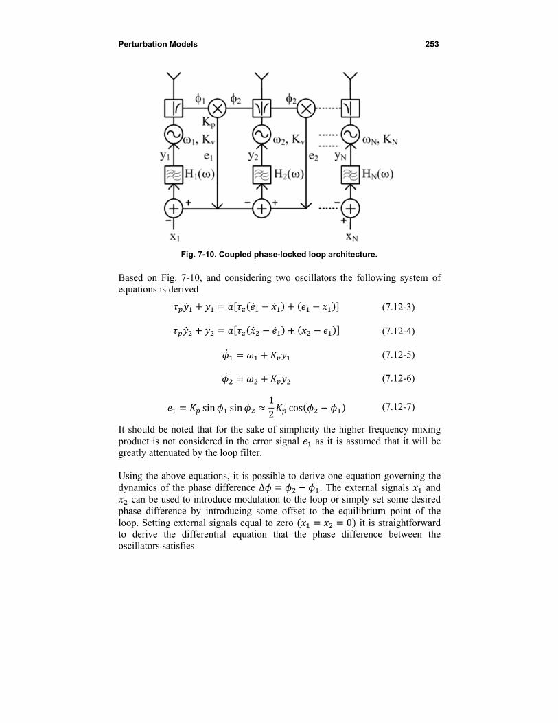
Perturbation M
Based on Figequations is d
It should be product is nogreatly attenu Using the abdynamics of
can be usphase differeloop. Settingto derive thoscillators sa
Models
Fig. 7-10. C
g. 7-10, and derived
sin
noted that foot considered uated by the l
bove equationthe phase died to introduence by intro
g external signhe differentiaatisfies
Coupled phase
considering
sin12
or the sake ofin the error
loop filter.
ns, it is possibfference Δ
uce modulatiooducing somenals equal to al equation t
e-locked loop
two oscillato
cos
f simplicity thsignal as
ble to derive . T
on to the loope offset to thzero
that the pha
architecture.
ors the follow
he higher freit is assumed
one equationThe external
p or simply sehe equilibrium
0 it is sase difference
25
wing system
(7.12-3)
(7.12-4)
(7.12-5)
(7.12-6)
(7.12-7)
equency mixind that it will b
n governing tsignals an
et some desirm point of tstraightforwae between th
53
of
ng be
the nd
red the ard the
254 Chapter 7
Δ 1 sin Δ Δ cos Δ Δ 0 (7.12-8)
where Δω and . The equilibrium points of the coupled PLL correspond to Δ Δ 0 and are derived by solving
cos Δ Δ 0 (7.12-9)
It is easy to verify that two solutions exist within the phase interval 0, 2 , and perturbation analysis of Eq. (7.12-8) can be used to show that only the one of the two that falls in the interval 0, is stable [127]. This fact implies that the phase difference of the two oscillators for the topology under consideration can be tuned in the range 0, , by varying the relative frequencies of the two oscillators Δ . The hold-in range Ω of the coupled PLL is the range of the frequency difference among the oscillator elements for which the system remains in a stable equilibrium. The pull-in range on the other hand, is the range of the frequency difference for which the system will eventually evolve to a stable equilibrium. The hold-in range presents an upper bound to the pull-in range. Based on the above analysis and the stability analysis of the equilibrium points, it was determined by Buckwalter, et al. [127] that the hold-in range is equal to
Ω 2G (7.12-10)
Furthermore, they calculated an approximate value for the pull-in range as given by Eq. 7.12-11 [127]
Ω 2
1 4τ G 1
2τ
(7.12-11)
Finally, Buckwalter, et al. [127] studied the effect of circuit delay on the hold-in and pull-in range of the system. Such delays are present in the system due to the filter characteristics of the circuit, and they result in complex dynamic behavior and instabilities. We remark that such filter characteristics may be fruitfully interpreted as time delays if the delay is small. Unlike Chapter 5 of this book, the analysis of Buckwalter, et al. does include the nonlinear behavior. Recall that in Chapter 5 we introduced coupling delay in oscillator arrays via an exponential of the Laplace transform variable. There the analysis was done in the linear approximation, and thus the solutions did not exhibit any of the complex dynamical behavior arising from nonlinearity. The delay introduced was a true time delay due to propagation through the coupling lines and was not constrained to be small. However, the late time behavior in that situation
Perturbation Models 255
corresponds to solution at time equal to many delay times, a condition which may be satisfied either by large t or small delay or both. The model described in this section can be made progressively more complex, by taking into account the high-frequency mixing product at the output of the phase detector in the formulation, or by using a higher order loop filter and digital phase detectors.
7.13 Conclusion
In this chapter we revisited the analysis of coupled-oscillator arrays and presented two approximate models that describe the amplitude and phase dynamics at the fundamental frequency of oscillation of the coupled oscillator arrays. We presented a compact matrix formulation of the models, which can be used to efficiently analyze the transient behavior of the arrays, determine the various steady-state solutions, and examine their stability. In addition we provided a formulation that enables one to consider external injection-locking signals to the array, which can be used to introduce modulation into the array. These models were used to provide an overview of the phase-noise analysis of coupled-oscillator arrays. Such approximate models can be used to simulate large coupled-oscillator arrays in a computationally efficient manner. Finally, it was pointed out that PLLs can be substituted for VCOs in coupled systems, resulting in behavior quite similar to that of the arrays discussed previously. In the next chapter we describe nonlinear simulation methods that can be used to accurately simulate and design oscillator circuits and coupled-oscillator arrays.

256 Chapter 7
257
Chapter 8 Numerical Methods for Simulating
Coupled Oscillator Arrays
Coupled-oscillator arrays present a challenge to the designer due to difficulties both in the accurate simulation of oscillator elements and in the requirement for computationally efficient simulation techniques for large arrays. In addition, coupled-oscillator array design is made more difficult by the presence of multiple operating modes and stability considerations. As a result, a number of approximations need to be used to reduce the simulation time. Such are describing function models for non-linear elements [15] [118] [129] [130], along with perturbation models, infinite array approximations and continuum models shown in Chapter 3 [38] [39] and in Chapter 4 [42] [43] [44], respectively. The progress in recent years in nonlinear simulation techniques has led to more accurate analysis and optimization methods for nonlinear circuits such as oscillators and mixers, as well as arrays [120,131]. Furthermore, these nonlinear simulation tools can be combined with electromagnetic simulation in order to analyze radiating structures and nonlinear antennas and arrays. In this chapter, an introduction to numerical methods for simulating nonlinear circuits is presented [132,131], focused on the simulation of autonomous circuits such as oscillators, followed by an introduction to convex optimization principles [133]. Nonlinear simulation techniques are demonstrated in order to trace the steady-state solutions of coupled-oscillator arrays and investigate their stability [116].
258 Chapter 8
8.1 Introduction to Numerical Methods
The recent advances in numerical methods for simulating nonlinear microwave circuits permit one to model oscillator and coupled-oscillator array circuits efficiently and accurately. In this section a brief introduction to the principles of commonly used methods will be presented, with an aim towards obtaining the periodic steady state of oscillator circuits. The reader is prompted to the literature for an advanced and detailed description of the various methods, such as for example Refs. [132,131,101,134]. Among the various existing numerical methods, transient simulation, harmonic balance, and envelope-transient simulation are described next.
8.1.1 Transient Simulation
A general nonlinear circuit is considered where a vector of size contains the state variables of the circuit, namely node voltages and currents. The circuit is described by a non-autonomous system of differential equations obtained by applying Kirchhoff’s current law at the circuit nodes as well as the voltage law at the circuit branches, as introduced in Eq. (7.1-2) and repeated here for convenience
, , (8.1-1)
with an initial condition , where typically 0. A vector of size including external, known, forcing terms has been included for generality.
The system is classified as an initial value problem [132], and the computation of its solution over a given time interval is known as transient simulation. There exist various discrete time numerical integration methods that are used to perform a transient simulation [101]. Assuming an integration time step , the values of the state variable vector at time are generally computed as follows [101]
, , (8.1-2)
The number of evaluations of the state variables and vector field that are required for the evaluation of the next state 1 are called the steps of the algorithm, and these steps define the order of the algorithm. An algorithm is called explicit if the future state depends only on past values of the state variables and the vector field, which corresponds to 0. If 0, the algorithm is called implicit. A commonly used single-step, explicit integration algorithm is the forward Euler algorithm, which is defined as
Numerical Methods for Simulating COAs 259
, , (8.1-3)
In contrast, the backward Euler algorithm is a single-step implicit algorithm
, , (8.1-4)
where the evaluation of the state vector at time 1 requires the computation of the vector field at the same time step. The resulting nonlinear system of algebraic equations maybe solved using some numerical root-finding algorithm. Typically the Newton-Raphson algorithm is used to compute the solution at each time step [132]. Assuming a nonlinear system of algebraic equations with unknown the steady state at time step 1 ,
, , (8.1-5)
the Newton-Raphson algorithm is an iterative algorithm that requires an initial guess as a starting point, and proceeds to find the roots of by calculating successive approximations of the unknown steady-state vector as
(8.1-6)
where j is the iteration index, and is the Jacobian of the nonlinear function [132]. The steady-state vector at the previous time step j is a good candidate for an initial guess . It can be shown that if the initial guess is close enough to a solution given by Eq. (8.1-5), if the nonlinear function is continuously differentiable, and the Jacobian is not singular, the sequence given by Eq. (8.1-6) converges to a root of . Many different numerical integration algorithms (8.1-2) exist depending on the choice of the various and coefficients. Selection of the appropriate integration algorithm depends on computational complexity, accuracy, and numerical stability considerations [101]. Moreover, modern integration routines adaptively adjust the integration step and order of the integration algorithm. In order to obtain the periodic steady state of an oscillator, one needs to integrate Eq. (8.1-1) for a sufficient time interval in order to allow all transient responses to decay. As a result, transient simulation is not an efficient method to analyze the behavior of oscillator and coupled oscillator systems. Conversely however, transient simulation provides a way to examine the stability of the solutions, as time-domain integration converges only to stable steady-state solutions. There exist time-domain algorithms such as the shooting methods that minimize the evaluation of the initial transient state in order to efficiently obtain the desired periodic steady state. In this case, one solves the system of
260 Chapter 8
differential equations given by Eq. (8.1-1) subject to a periodic boundary condition , where is the period of the steady state. The reader is prompted to the literature for a description of these methods [101,132].
8.1.2 Harmonic Balance Simulation
Frequency domain methods are particularly suited for the analysis of systems where a periodic solution exists. In this case it is possible to represent the steady-state solution by a trigonometric polynomial of degree . The selected value of is a trade-off between accuracy and computational efficiency. Specifically, assuming a state vector of size , and a vector of external forcing signals of size , we can write
(8.1-7)
(8.1-8)
where is the angular fundamental frequency of the periodic steady state. The frequency domain state vector and external forcing signal vector are defined by the by 2 1 matrix , and by the by 2 1 matrix , respectively. Similarly, the vector field , , is a periodic function and can also be expanded in a Fourier series as
, , , (8.1-9)
where , is the frequency domain vector field by 2 1 matrix, and depends both on and . In a typical piecewise harmonic balance algorithm implementation [134], the circuit is divided into a linear sub-circuit and a nonlinear sub-circuit, and Kirchhoff’s laws are applied in the nodes that connect the two sub-circuits. The response of the nonlinear sub-circuit is computed in the time domain and a fast Fourier transform algorithm is used to convert the related data to the frequency domain. As a result, in order to compute the frequency domain vector field matrix , one first applies the inverse Fourier transform to the state and external signal vectors in order to obtain their time-domain expressions and
, then computes the time-domain vector field , , , and finally applies the Fourier transform to , , in order to obtain .
Numerical Methods for Simulating COAs 261
By introducing Eqs. (8.1-7), (8.1-8) and (8.1-9) into the original time-domain system of differential equations given by Eq. (8.1-1), and balancing the coefficients of the exponential terms , a system of algebraic equations is obtained
, , (8.1-10)
The matrix contains the angular frequency terms generated by the time derivative operation on the Fourier series expansion in Eq. (8.1-7). The above system of algebraic equations is efficiently solved using root finding algorithms such as for example the Newton-Raphson algorithm [134,132] described in the previous section. It should be noted, that when the steady state is expanded using only a first-order trigonometric polynomial ( 1), the corresponding formulation is known as the describing function [131], and it can be used to obtain insightful analytical expressions. The coupled-oscillator models of the previous chapter are describing function formulations. Harmonic balance is able to handle quasi-periodic solutions by properly extending the polynomial basis and the time to a frequency-domain transform algorithm [132].
8.1.3 Conversion Matrix
In microwave mixer circuits, a quasi-periodic steady-state solution exists with two or more fundamental frequency components. In the simplest scenario, two fundamental frequencies need to be considered corresponding to the local oscillator signal and the RF input signal to the mixer. Correspondingly, a two-fundamental-frequency harmonic balance algorithm needs to be used in order to evaluate the steady state. However, in typical mixer operation, the local oscillator signal has significantly larger power than the RF input to the mixer. As a result, it is possible to evaluate the periodic steady state in the absence of the RF input signal, defined by the local oscillator signal and using a harmonic balance algorithm with a single fundamental-frequency component. The effect of the RF input signal is then considered as a linear perturbation of the previously defined steady state leading to a computationally efficient algorithm known as the conversion matrix method. Assuming a linear perturbation of the steady-state solution
, and an external RF signal , the initial system of differential equations becomes
262 Chapter 8
, , (8.1-11)
, , , ,
where is the solution that corresponds to the large local-oscillator signal in the absence of the RF input, and and are the time-varying Jacobians of the vector field versus the state vector and versus the input RF signal vector , respectively, evaluated at and 0. Both equations of the above system are solved in the frequency domain by applying the harmonic balance algorithm as Eq. (8.1-10). The frequency domain coefficients of the Jacobian matrices involved in the second equation are obtained at no additional computational cost during the Newton-Raphson harmonic balance computation of the large signal steady state corresponding to the first equation of Eq. (8.1-11) [131] [134].
8.1.4 Envelope Transient Simulation
The envelope transient simulation is a combination of the transient and harmonic balance simulation methods proposed D. Sharrit [135] and E. Ngoya and R. Larcheveque [136]. In effect, one represents the state variables, external forcing terms, and vector field by Fourier-series expansions of time-varying phasors
(8.1-12)
(8.1-13)
, , , (8.1-14)
Consequently, a transformed system of differential equations is obtained that has the form
, , (8.1-15)
The above system is solved using time-domain integration. The advantage of envelope transient simulation over the traditional transient simulation is that the time-varying phasors are slowly varying, allowing one to use a much larger time step in the simulation. Being a time-domain simulation, envelope
Numerical Methods for Simulating COAs 263
transient simulation may also be used to verify the stability of a steady-state solution as it converges only to stable solutions.
8.1.5 Continuation Methods
Once a steady-state solution is obtained, continuation methods can be used to obtain the families of steady-state solutions that occur as one or more parameters of the circuit under consideration are varied. Continuation techniques provide an initial condition that is close to the required steady-state solution, so that the application of the Newton-Raphson or any other root finding algorithm that is being used converges quickly and efficiently. Assuming a parameter for which the steady-state solution has been evaluated, it is then possible to obtain the steady-state solution corresponding to the parameter value by considering a sequence of values … and progressively evaluating the steady state corresponding to each parameter value by using the solution at each step as the initial condition for the evaluation of the next step [132]. In order to reduce the steps of the continuation method, the already obtained steady-state values are extrapolated. Assuming that the steady-state solution at step has been obtained by solving the harmonic balance system Eq. (8.1-10),
, 0 (8.1-16)
the solution corresponding to is approximated by linear extrapolation as
0 (8.1-17)
where is the Jacobian matrix of the harmonic balance system. The above matrix equation can be solved in order to obtain an initial condition for the state vector
(8.1-18)
Continuation methods based on Eq. (8.1-18) may fail due to singularities in the Jacobian matrix ⁄ , which result from the existence of multiple solutions versus the parameter under consideration. In this case, tracing of the steady-state solutions can be accomplished by parameter switching [137]. Parameter switching corresponds to tracing the steady-state solutions versus another, different circuit parameter or steady-state variable, for which the corresponding Jacobian matrix is not singular.
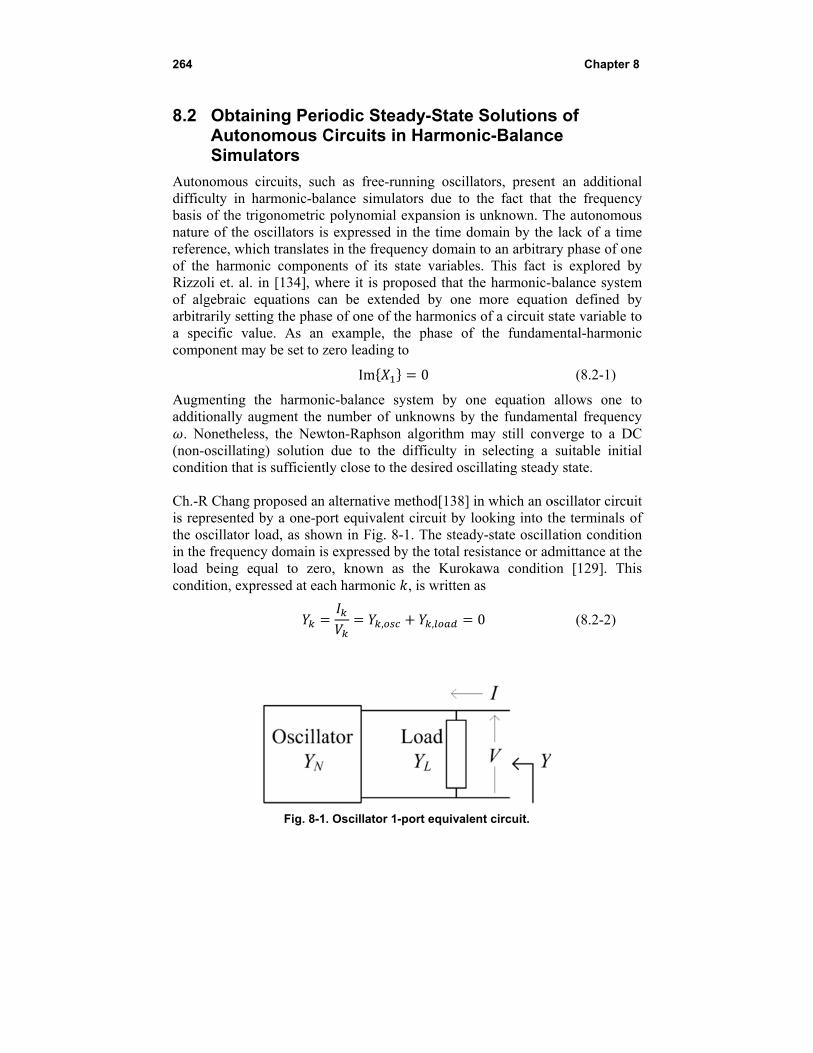
264
8.2 ObtaAutoSimu
Autonomousdifficulty in basis of the tnature of thereference, whof the harmoRizzoli et. alof algebraic arbitrarily seta specific vcomponent m
Augmenting additionally
. Nonethele(non-oscillaticondition tha Ch.-R Changis representedthe oscillatorin the frequenload being econdition, ex
aining Peronomous Culators
circuits, sucharmonic-ba
trigonometrice oscillators ishich translateonic componl. in [134], w
equations ctting the phas
value. As an may be set to z
the harmonaugment the ess, the Newing) solutionat is sufficient
g proposed and by a one-por load, as shoncy domain isequal to zer
xpressed at ea
Fig. 8-1
riodic SteaCircuits in
ch as free-rualance simulac polynomial s expressed is in the frequ
nents of its swhere it is pro
an be extendse of one of th
example, thzero leading t
Im
nic-balance synumber of u
wton-Raphson due to the tly close to th
n alternative mort equivalen
own in Fig. 8-s expressed bro, known asch harmonic
,
. Oscillator 1-
ady-State n Harmon
unning oscillaators due to expansion is n the time do
uency domain tate variables
oposed that thded by one he harmonicshe phase of to
0
ystem by onunknowns by n algorithm m
difficulty in he desired osc
method[138] int circuit by lo-1. The stead
by the total ress the Kurok
, is written a
,
-port equivale
Solutionsic-Balanc
ators, presentthe fact that unknown. Th
omain by theto an arbitrar
s. This fact he harmonic-bmore equati of a circuit sthe fundam
ne equation the fundame
may still convselecting a
illating steady
in which an oooking into th
dy-state oscillsistance or ad
kawa conditioas
0
nt circuit.
Chapter
s of ce
t an additionthe frequen
he autonomoe lack of a timry phase of onis explored bbalance systeion defined bstate variable
mental-harmon
(8.2-1)
allows one ental frequenverge to a Dsuitable initiy state.
oscillator circuhe terminals lation conditiodmittance at thon [129]. Th
(8.2-2)
r 8
nal ncy ous me ne by em by to
nic
to cy
DC ial
uit of on the his
Numerical Methods for Simulating COAs 265
Enforcing the above condition in addition to the harmonic balance system enables the algorithm to avoid converging to solutions corresponding to zero harmonic components and , such as the non-oscillating DC solution. In fact, in order to avoid the DC solution, it is necessary to impose the admittance condition only at the fundamental harmonic component [138]
0 (8.2-3)
which leads to two additional real equations in the harmonic balance system
Re 0 (8.2-4)
Im 0
As a result, two additional variables can be introduced to the extended harmonic balance system, the unknown frequency , and oscillation amplitude
at the load. The additional advantage of this formulation is that the designer may impose in a circuit optimization problem the desired oscillation frequency and amplitude at the load. A dual formulation may also be obtained by considering a series one-port equivalent circuit and enforcing the oscillation condition by setting the total impedance equal to zero. The condition given by Eq. (8.2-3) was implemented by R. Quere, et al. in commercial simulators [139], allowing for a practical design and optimization methodology for autonomous circuits. According to Ref. [139], one needs to introduce into the simulator an ideal probe circuit such as the one shown in Fig. 8-2. The probe is connected in parallel to a selected circuit node and consists of an ideal sinusoidal source of a given amplitude , phase , and frequency , connected in series with a current meter and an ideal filter. The filter is such that it presents infinite impedance for frequencies other than the ideal source frequency , thus restricting the effect of the probe to . In free-running oscillator simulation, the phase of the probe is set to an arbitrary but fixed value, for example zero. An optimization loop is run in order to find the nonzero amplitude and frequency of the probe that correspond to zero admittance ⁄ . Each iteration of the loop is a harmonic-balance analysis. The result , of the optimization defines the oscillating steady state. Alternatively, in the case of an externally injection-locked oscillator, the frequency is known and corresponds to the frequency of the external source. In this case, the pair , represents the unknowns of the optimization loop, as the oscillation phase is not arbitrary any more; rather, it depends on the injection source.
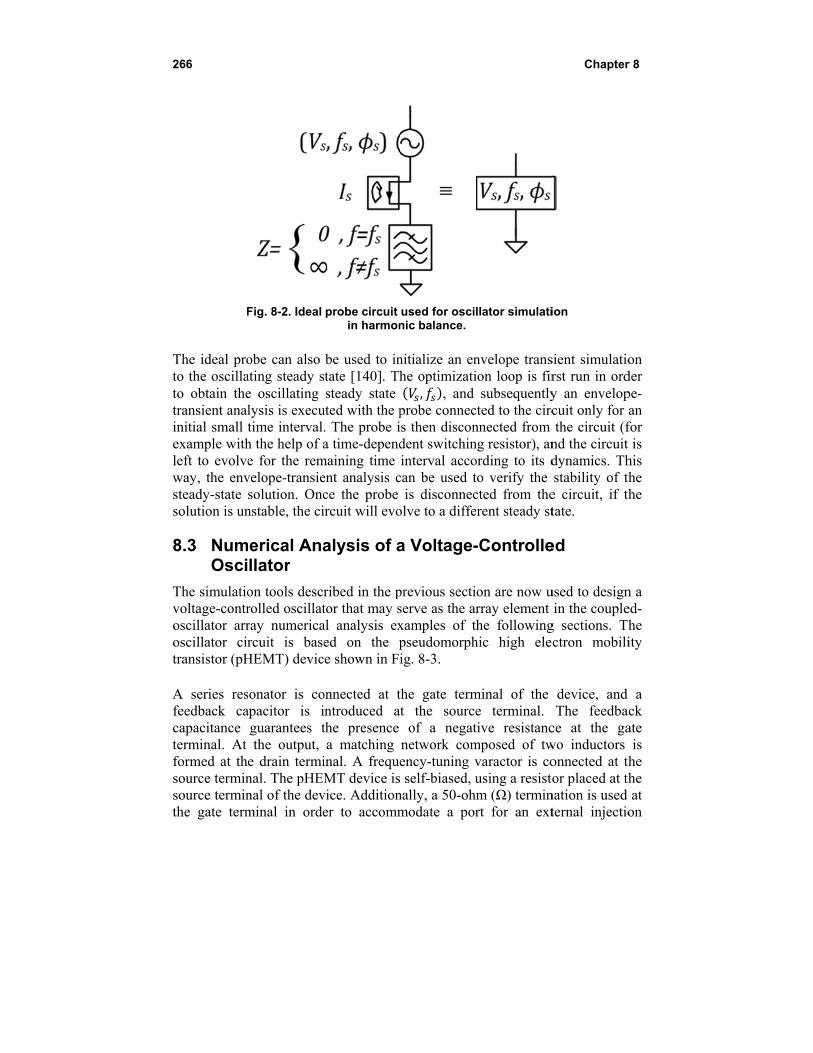
266
F
The ideal proto the oscillato obtain thetransient analinitial small texample withleft to evolveway, the envsteady-state solution is un
8.3 NumOsci
The simulatiovoltage-controscillator arroscillator cirtransistor (pH A series resfeedback cacapacitance terminal. At formed at thsource terminsource terminthe gate term
Fig. 8-2. Ideal
obe can also ating steady se oscillating lysis is executime interval.h the help of ae for the rem
velope-transiesolution. Oncnstable, the ci
merical Anallator
on tools descrrolled oscillatray numericarcuit is base
HEMT) devic
sonator is coapacitor is i
guarantees tthe output,
e drain terminal. The pHEMnal of the devminal in orde
probe circuit in harmon
be used to instate [140]. Thsteady state
uted with the p. The probe ia time-depend
maining time ent analysis cce the probe ircuit will evo
alysis of a
ribed in the ptor that may sal analysis exed on the pe shown in Fi
onnected at tintroduced athe presence a matching
inal. A frequeMT device is
vice. Additioner to accomm
used for oscinic balance.
nitialize an enhe optimizati
, , and probe connecis then discondent switchininterval acco
can be used tis disconnec
olve to a diffe
a Voltage-
previous sectiserve as the arxamples of tpseudomorphig. 8-3.
the gate termat the source
of a negatnetwork comency-tuning v
s self-biased, unally, a 50-ohmmodate a por
llator simulati
nvelope transion loop is fir
subsequentlycted to the circnnected from ng resistor), anording to its dto verify the cted from theerent steady st
-Controlle
on are now urray element he following
hic high ele
minal of the e terminal. tive resistancmposed of twvaractor is cousing a resistom (Ω) terminrt for an ext
Chapter
ion
sient simulatiorst run in ordy an envelopcuit only for the circuit (f
nd the circuit dynamics. Thstability of th
e circuit, if thtate.
ed
used to designin the couple
g sections. Thctron mobili
device, and The feedba
ce at the gawo inductors onnected at thor placed at th
nation is used ternal injectio
r 8
on der pe-an for t is his the the
n a ed-he ity
a ack ate
is the the
at on
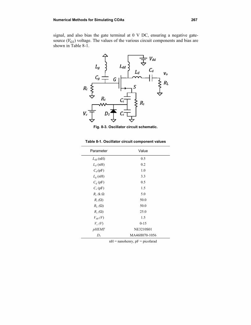
Numerical Me
signal, and asource ( ) shown in Tab
ethods for Sim
also bias the voltage. The
ble 8-1.
Fig.
Table 8-1
Param
Ldd (n
Ld (n
Cd (p
Lg (n
Cg (p
Cs (p
Rc (k
Ri (Ω
RL (Ω
Rs (Ω
Vdd (
Vc (
pHEM
D1
mulating COAs
gate terminavalues of the
8-3. Oscillato
1. Oscillator c
meter
nH)
nH)
pF)
nH)
pF)
pF)
k Ω
Ω)
(Ω)
Ω)
(V)
(V)
MT
1
nH = nano
s
al at 0 V DCe various circ
or circuit sche
ircuit compon
Value
0.5
0.2
1.0
3.3
0.5
1.5
5.0
50.0
50.0
25.0
1.5
0-15
NE3210S
MA46H070
ohenry, pF = pic
C, ensuring a uit componen
matic.
nent values
e
S01
0-1056
cofarad
26
negative gatnts and bias a
67
te-are
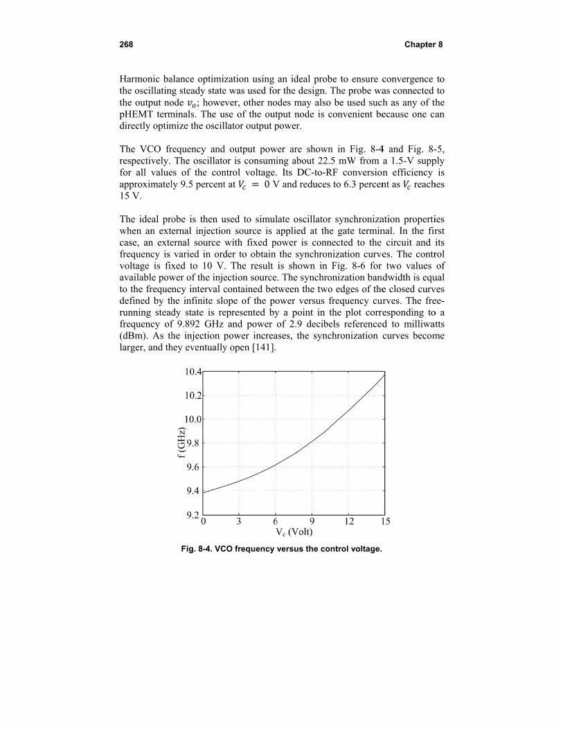
268
Harmonic bathe oscillatinthe output nopHEMT termdirectly optim The VCO frrespectively. for all valueapproximatel15 V. The ideal prowhen an extcase, an extefrequency is voltage is fixavailable powto the frequedefined by thrunning steadfrequency of(dBm). As thlarger, and th
alance optimig steady stateode ; howeminals. The umize the oscil
requency andThe oscillato
es of the conly 9.5 percent
obe is then uernal injectioernal source varied in ord
xed to 10 Vwer of the injency interval che infinite slody state is ref 9.892 GHz he injection phey eventually
Fig. 8-4. VC
zation using e was used foever, other nouse of the outllator output p
d output powor is consumintrol voltage.t at 0 V
used to simulon source is awith fixed pder to obtain . The result ection sourcecontained betope of the poepresented by
and power power increay open [141].
CO frequency v
an ideal probr the design.
odes may alsotput node is cpower.
wer are showning about 22. Its DC-to-R
V and reduces
late oscillatorapplied at theower is connthe synchronis shown in . The synchrotween the twoower versus fy a point in tof 2.9 decibe
ases, the sync
versus the co
be to ensure cThe probe wa
o be used succonvenient be
n in Fig. 8-4.5 mW fromRF conversios to 6.3 percen
r synchronizae gate termin
nected to the nization curveFig. 8-6 for
onization bano edges of thefrequency cuthe plot correels referencedchronization
ontrol voltage.
Chapter
convergence as connected h as any of thecause one c
4 and Fig. 8-a 1.5-V suppn efficiency nt as reach
ation propertinal. In the fir
circuit and es. The contrtwo values
ndwidth is eque closed curv
urves. The freesponding tod to milliwatcurves becom
r 8
to to
the an
-5, ply
is hes
ies rst its rol of
ual ves ee-o a atts me
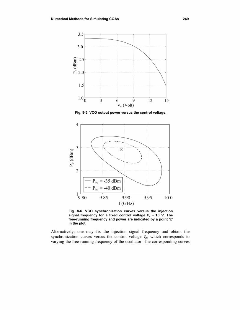
Numerical Me
Figsigfrein t
Alternativelysynchronizativarying the f
ethods for Sim
Fig. 8-5. VCO
g. 8-6. VCO sgnal frequencye-running freqthe plot.
y, one may ion curves vfree-running f
mulating COAs
O output powe
synchronizatioy for a fixed quency and p
fix the injecversus the cofrequency of
s
er versus the c
on curves vecontrol volta
ower are indic
ction signal ontrol voltage
the oscillator
control voltag
ersus the injeage Vcated by a po
frequency ae , which r. The corresp
26
ge.
ection V. The oint ‘x’
and obtain thcorresponds ponding curv
69
the to
ves
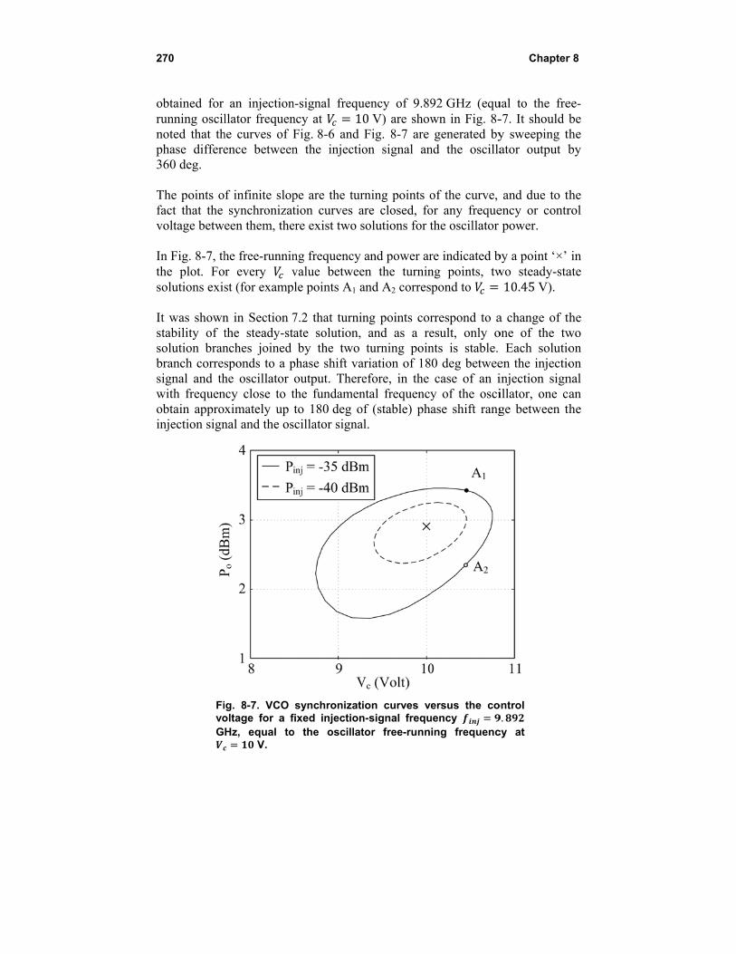
270
obtained for running oscilnoted that thphase differe360 deg. The points ofact that the voltage betw In Fig. 8-7, ththe plot. Fosolutions exis It was shownstability of tsolution branbranch corressignal and thwith frequenobtain approinjection sign
FivoG
an injectionllator frequen
he curves of Fence between
f infinite slopsynchronizat
een them, the
he free-runninr every vst (for examp
n in Section 7the steady-stnches joined sponds to a phe oscillator ncy close to tximately up nal and the os
ig. 8-7. VCO oltage for a fHz, equal to
V.
n-signal frequncy at 1Fig. 8-6 and n the injectio
pe are the turtion curves aere exist two s
ng frequency value betwee
ple points A1 a
7.2 that turniate solution, by the two
phase shift vaoutput. Therethe fundamento 180 deg o
scillator signa
synchronizatfixed injectiono the oscillat
uency of 9.890V) are showFig. 8-7 are on signal an
rning points oare closed, fosolutions for t
and power aren the turninand A2 corres
ng points corand as a returning poin
ariation of 18efore, in the ntal frequencyof (stable) phaal.
ion curves ven-signal frequtor free-runn
92 GHz (equwn in Fig. 8-generated by
nd the oscilla
of the curve,or any frequethe oscillator
re indicated bng points, twpond to
rrespond to aesult, only onts is stable. 0 deg betweecase of an i
y of the osciase shift rang
ersus the couency ing frequenc
Chapter
ual to the fre-7. It should by sweeping thator output b
and due to thency or contrpower.
by a point ‘×’ wo steady-sta10.45V).
a change of tone of the tw
Each solutioen the injectioinjection signillator, one cge between th
ontrol .
cy at
r 8
ee-be
the by
the rol
in ate
the wo on on nal an
the

Numerical Me
It is possiblepoint on it anstate solutionsignal power3.4 dBm, reswas examin100 nanosecodomain integcan see that tof Fig. 8-7 isof Fig. 8-6 is Finally, it shperturbation arrays, can bsingle elemeoscillator circprobe admittlooking into can be evaluderivatives fdefined by amplitude 0.4
ethods for Sim
to determinend running ann as was desr of –35 dBmspectively, coned by enveonds (ns) andgration algoritthe system evs stable. In a s the stable on
hould be notmodel of S
be easily comnt with an idcuit admittantance. Once the probe haated using finfor the oscillcontrol volta
442 V (
Fig. 8-8. Envstate correspand the syste
mulating COAs
e which one on envelope trscribed in Se, the points Arrespond to
elope transied a time stepthm [101]. Tholves to pointsimilar way, o
ne.
ted that the ection 7.6 thmputed fromdeal probe plce derivativethe steady s
as been deternite differenclator of Fig.age 102.9 dBm) are
velope-transieponding to A2
em evolves to
s
of the brancheansient analyction 8.2. Fo
A1 and A2 of o10.45 (F
ent simulatiop of 5 ns wehe result is sht A1, demonstone can also
oscillator admat is used to
m a harmoniclaced at the ds are equal tostate correspmined, the p
ces [116]. As 8-3, corresp0 V, frequee listed in Tab
ent analysis 2 of Fig. 8-7. A1.
es is stable bysis initializedr example, foutput power
Fig. 8-7). Theon. A simulere used, withhown in Fig.trating that thverify that th
mittance derio model couc-balance simdesired oscillo the derivativonding to zerobe admittanan example,
ponding to thncy 9.
ble 8-2.
of the steadA2 is unstabl
27
y selecting od to the steadfor an injectior 2.35 dBm ane stability of Alation time h a Gear tim8-8, where on
he upper branhe upper bran
ivatives of tupled oscillatmulation of thlator node. Tves of the ideero admittannce derivativthe admittan
he steady sta892GHz, an
dy le
71
ne dy-on nd A2 of
me-ne
nch nch
the tor the he eal nce ves nce ate nd
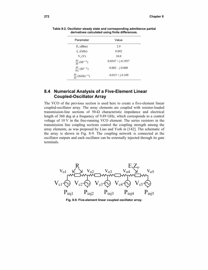
272
Table 8-
8.4 NumCoup
The VCO ofcoupled-osciltransmission-length of 360voltage of 10transmission array elementhe array is oscillator outterminals.
-2. Oscillator sderivativ
Param
Po (dB
fo (GH
Vc (V
(S
(S
(S
merical Anapled-Osci
f the previousllator array. -line section0 deg at a fre0 V in the frline couplin
nts, as was prshown in F
tputs and each
Fig. 8-9. Five
steady state aves calculated
meter
Bm)
Hz)
V)
)
)
)
alysis of allator Arra
s section is uThe array eles of 50-Ω c
equency of 9.ee-running V
ng sections coroposed by LiFig. 8-9. Theh oscillator c
e-element line
and correspon using finite d
Value
2.9
9.892
10.0
0.0547 + j 0
0.002 – j 0
-0.015 + j 0
a Five-Eleay
used here to ements are ccharacteristic89 GHz, whi
VCO elementontrol the coiao and York coupling nean be externa
ear coupled os
nding admittandifferences.
e
2
0.1957
0.008
0.109
ment Line
create a five-coupled with impedance ich correspon. The series roupling strenk in [142]. Thetwork is coally injected t
scillator array
Chapter
nce partial
ear
-element lineresistor-loadand electric
nds to a contrresistors in thgth among th
he schematic onnected at ththrough its ga
y.
r 8
ear ded cal rol the the of
the ate
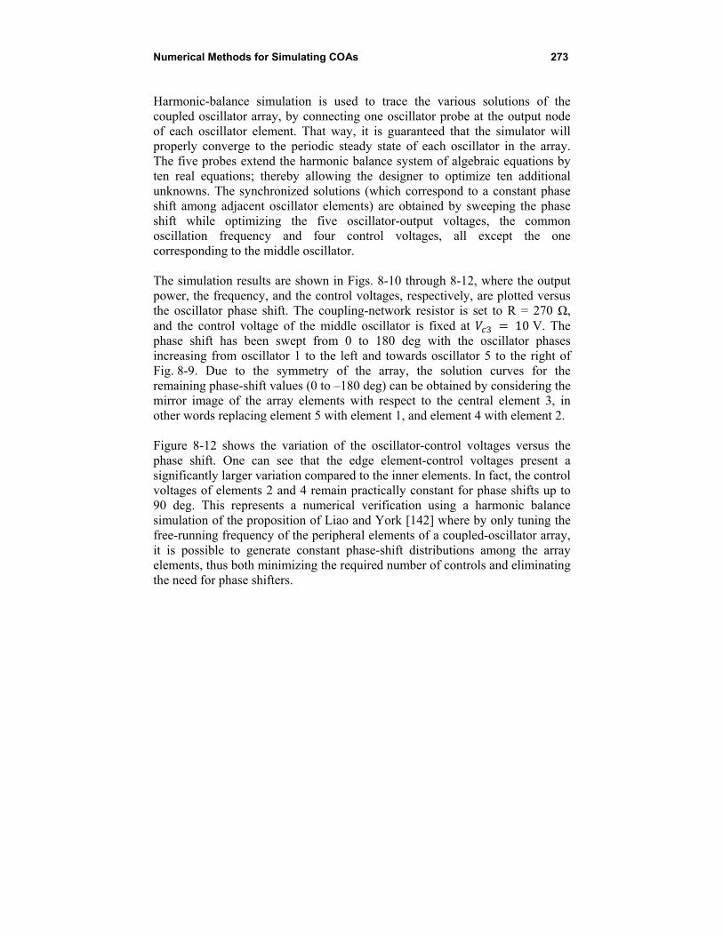
Numerical Methods for Simulating COAs 273
Harmonic-balance simulation is used to trace the various solutions of the coupled oscillator array, by connecting one oscillator probe at the output node of each oscillator element. That way, it is guaranteed that the simulator will properly converge to the periodic steady state of each oscillator in the array. The five probes extend the harmonic balance system of algebraic equations by ten real equations; thereby allowing the designer to optimize ten additional unknowns. The synchronized solutions (which correspond to a constant phase shift among adjacent oscillator elements) are obtained by sweeping the phase shift while optimizing the five oscillator-output voltages, the common oscillation frequency and four control voltages, all except the one corresponding to the middle oscillator. The simulation results are shown in Figs. 8-10 through 8-12, where the output power, the frequency, and the control voltages, respectively, are plotted versus the oscillator phase shift. The coupling-network resistor is set to R = 270 Ω, and the control voltage of the middle oscillator is fixed at 10 V. The phase shift has been swept from 0 to 180 deg with the oscillator phases increasing from oscillator 1 to the left and towards oscillator 5 to the right of Fig. 8-9. Due to the symmetry of the array, the solution curves for the remaining phase-shift values (0 to –180 deg) can be obtained by considering the mirror image of the array elements with respect to the central element 3, in other words replacing element 5 with element 1, and element 4 with element 2. Figure 8-12 shows the variation of the oscillator-control voltages versus the phase shift. One can see that the edge element-control voltages present a significantly larger variation compared to the inner elements. In fact, the control voltages of elements 2 and 4 remain practically constant for phase shifts up to 90 deg. This represents a numerical verification using a harmonic balance simulation of the proposition of Liao and York [142] where by only tuning the free-running frequency of the peripheral elements of a coupled-oscillator array, it is possible to generate constant phase-shift distributions among the array elements, thus both minimizing the required number of controls and eliminating the need for phase shifters.
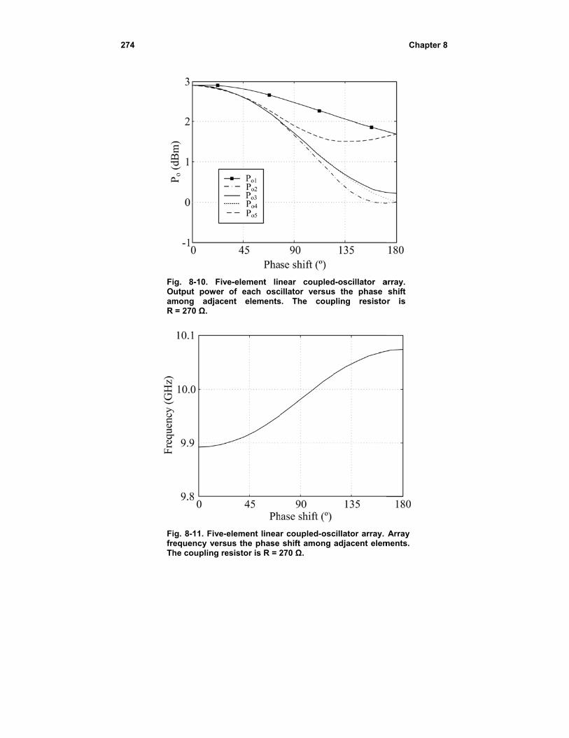
274
FiOamR
FifreTh
ig. 8-10. Fivutput power mong adjace= 270 Ω.
ig. 8-11. Five-eequency vershe coupling re
ve-element linof each osc
ent elements
element lineaus the phase
esistor is R = 2
near coupledcillator versuss. The coup
r coupled-oscshift among
270 Ω.
d-oscillator as the phase pling resisto
cillator array. adjacent elem
Chapter
array. shift
or is
Array ments.
r 8
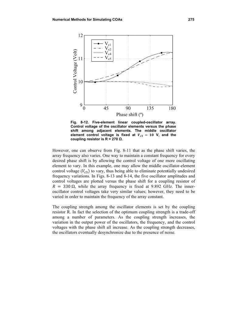
Numerical Me
FigCoshielecou
However, onarray frequendesired phaseelement to vacontrol voltafrequency vacontrol volta 330Ω,
oscillator convaried in ord The couplingresistor R. Inamong a nuvariation in tvoltages withthe oscillator
ethods for Sim
g. 8-12. Fiventrol voltage ift among a
ement controlupling resisto
ne can observncy also variee shift is by ary. In this exge ( to va
ariations. In Fages are plott, while the antrol voltageser to maintain
g strength amn fact the seleumber of pathe output poh the phase srs eventually d
mulating COAs
e-element linof the oscilla
adjacent eleml voltage is f
or is R = 270 Ω
ve from Fig. es. One way to
allowing thexample, one ary, thus bein
Figs. 8-13 andted versus tharray frequens take very sn the frequenc
mong the oscection of the arameters. Asower of the oshift all incredesynchroniz
s
near coupledator elements ments. The fixed at
Ω.
8-11 that aso maintain a c
control voltamay allow th
ng able to elimd 8-14, the fivhe phase shiftncy is fixed imilar valuescy of the array
cillator elemeoptimum cous the coupliscillators, thease. As the ce due to the p
d-oscillator aversus the pmiddle oscil V, and
s the phase sconstant frequage of one mhe middle oscminate potentve oscillator aft for a coupl
at 9.892 GHs; however, thy constant.
ents is set byupling strengting strength e frequency, acoupling strenpresence of no
27
array. hase llator
d the
shift varies, thuency for eve
more oscillatincillator-elemetially undesiramplitudes anling resistor Hz. The innehey need to b
y the couplinth is a trade-o
increases, thand the contrngth decreaseoise.
75
the ery ng ent red nd of
er-be
ng off the rol es,
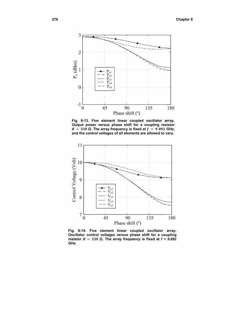
276
FiO
an
Fig. OscresiGHz
ig. 8-13. Fiveutput power
Ω. Thnd the control
8-14. Five cillator controstor z.
e element linversus phasee array freque voltages of a
element linl voltages ve Ω. The array
near couplede shift for a ency is fixed aall elements ar
near coupledrsus phase sy frequency is
oscillator acoupling res
at . re allowed to v
d oscillator shift for a cous fixed at f =
Chapter
array. sistor GHz, vary.
array. upling 9.892
r 8
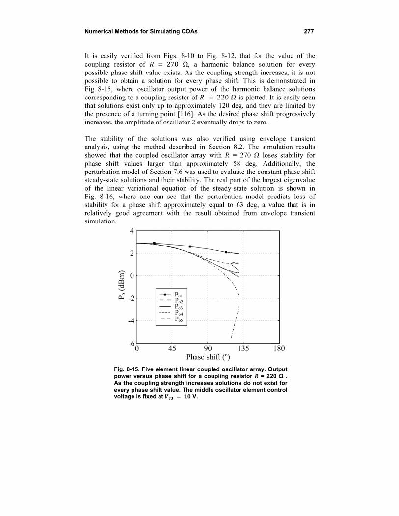
Numerical Me
It is easily vcoupling respossible phapossible to oFig. 8-15, whcorrespondinthat solutionsthe presence increases, the The stabilityanalysis, usinshowed that phase shift perturbation steady-state sof the linearFig. 8-16, wstability for relatively gosimulation.
FigpowAs evevol
ethods for Sim
verified fromsistor of se shift valueobtain a soluhere oscillato
ng to a couplis exist only uof a turning
e amplitude o
y of the solng the methothe coupled values large
model of Secsolutions andr variational
where one caa phase shif
ood agreemen
g. 8-15. Five ewer versus phthe coupling
ery phase shifltage is fixed a
mulating COAs
m Figs. 8-10270 Ω, a
e exists. As tution for everor output pong resistor ofup to approxipoint [116]. f oscillator 2
lutions was od describedoscillator ar
er than appction 7.6 was d their stability
equation ofan see that tft approximatnt with the r
lement linear hase shift forstrength incr
ft value. The mat V
s
to Fig. 8-12a harmonic bthe coupling ry phase shiwer of the hf 220 Ωimately 120 dAs the desireeventually dr
also verifiedd in Section rray with =proximately 5
used to evaluy. The real p
f the steady-the perturbatitely equal to result obtaine
coupled oscir a coupling rereases solutiomiddle oscilla
V.
2, that for thbalance solutstrength incrft. This is dharmonic balΩ is plotted. Ideg, and theyed phase shifrops to zero.
d using enve8.2. The sim= 270 Ω los58 deg. Aduate the constart of the largstate solutionion model p63 deg, a v
ed from env
llator array. Oesistor = 22
ons do not exitor element co
27
he value of thution for evereases, it is n
demonstrated lance solutioIt is easily se
y are limited bft progressive
elope transiemulation resu
es stability fdditionally, thtant phase shgest eigenvalun is shown
predicts loss value that is velope transie
Output 20 Ω . ist for ontrol
77
the ery not
in ons en by ely
ent ults for the hift ue in of in
ent
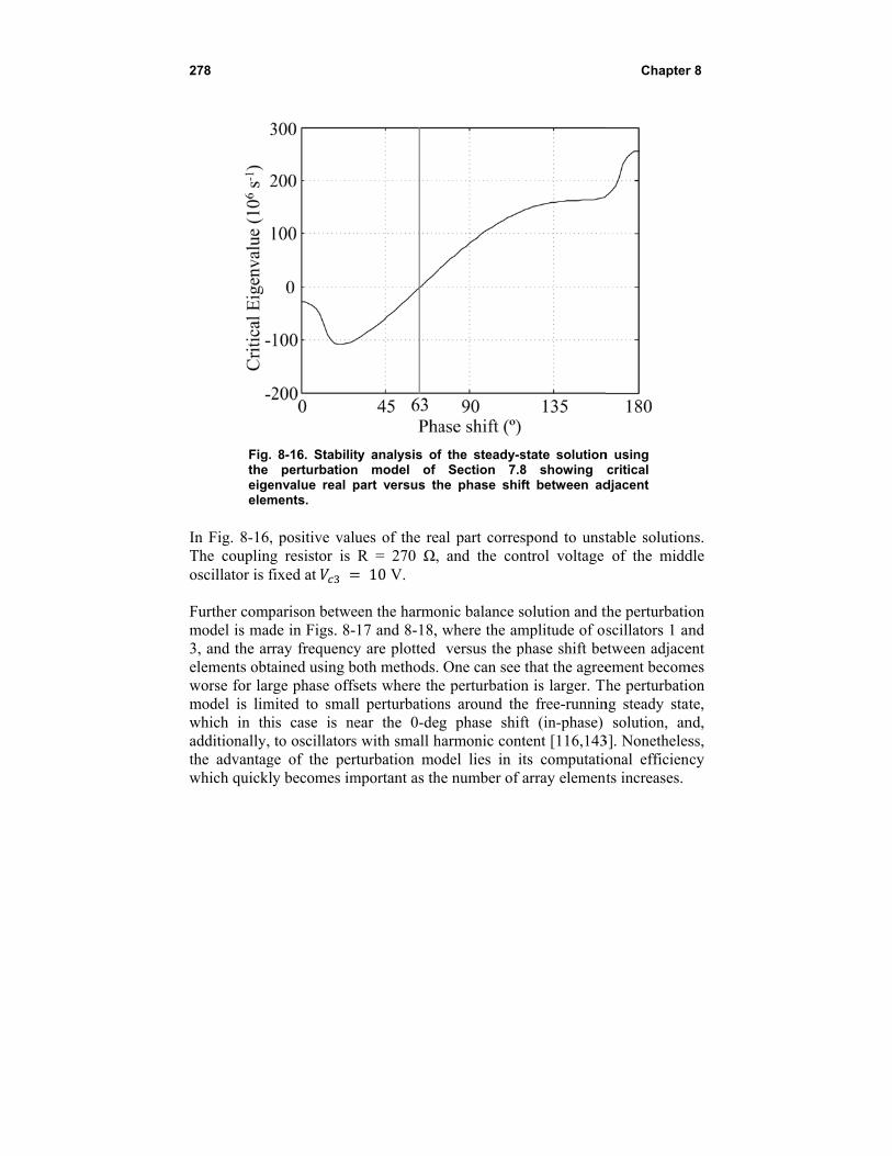
278
Fig. theeigeelem
In Fig. 8-16,The couplingoscillator is f Further compmodel is mad3, and the arelements obtaworse for larmodel is limwhich in thiadditionally, the advantagwhich quickl
8-16. Stabilitperturbation
envalue real pments.
, positive valug resistor is fixed at
parison betwede in Figs. 8-ray frequencyained using brge phase offs
mited to smalis case is neto oscillators
ge of the perly becomes im
ty analysis ofn model of part versus th
ues of the reR = 270 Ω,10 V.
een the harmo17 and 8-18,y are plotted
both methods.sets where thl perturbationear the 0-des with small hrturbation momportant as th
f the steady-sSection 7.8
he phase shif
al part corres and the con
onic balance swhere the am versus the p One can see e perturbationns around theg phase shif
harmonic contodel lies in ihe number of
state solution8 showing ft between ad
spond to unstntrol voltage
solution and tmplitude of ophase shift be
that the agreen is larger. The free-runninft (in-phase) tent [116,143ts computatioarray element
Chapter
n using critical
djacent
table solutionof the midd
the perturbatioscillators 1 an
etween adjaceement becomhe perturbatio
ng steady statsolution, an
3]. Nonethelesonal efficien
nts increases.
r 8
ns. dle
on nd ent
mes on te,
nd, ss, cy
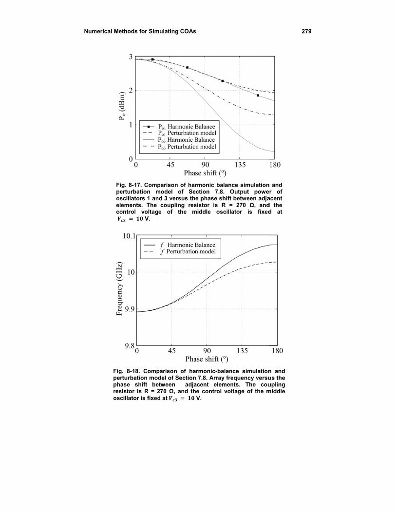
Numerical Me
Fipeoselco
Figperpharesosc
ethods for Sim
ig. 8-17. Comperturbation mscillators 1 anements. The
ontrol voltag V.
g. 8-18. Comprturbation moase shift be
sistor is R = 2cillator is fixed
mulating COAs
parison of hamodel of Send 3 versus th
coupling resge of the m
parison of hadel of Section
etween adja270 Ω, and thd at
s
rmonic balanection 7.8. Ohe phase shift sistor is R =
middle oscilla
armonic-balann 7.8. Array freacent elemenhe control vol
V.
ce simulationOutput powe
between adja= 270 Ω, andator is fixed
nce simulationequency versunts. The coultage of the m
27
n and er of acent d the d at
n and us the upling middle
79
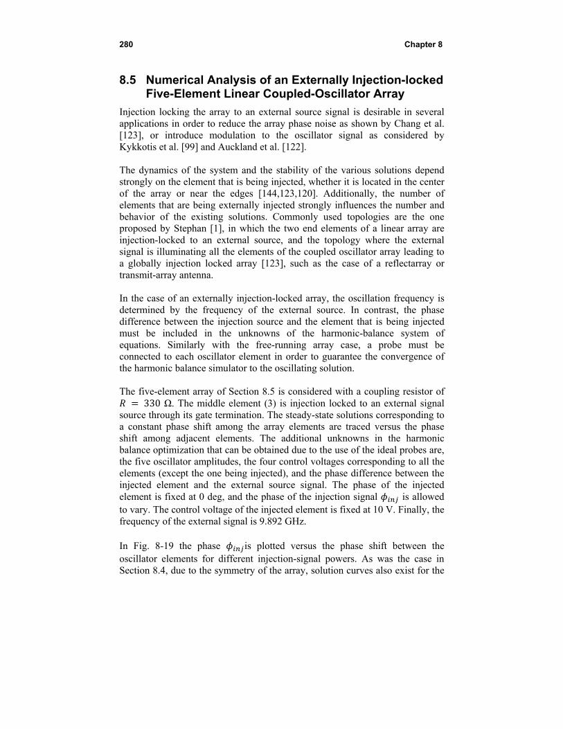
280 Chapter 8
8.5 Numerical Analysis of an Externally Injection-locked Five-Element Linear Coupled-Oscillator Array
Injection locking the array to an external source signal is desirable in several applications in order to reduce the array phase noise as shown by Chang et al. [123], or introduce modulation to the oscillator signal as considered by Kykkotis et al. [99] and Auckland et al. [122]. The dynamics of the system and the stability of the various solutions depend strongly on the element that is being injected, whether it is located in the center of the array or near the edges [144,123,120]. Additionally, the number of elements that are being externally injected strongly influences the number and behavior of the existing solutions. Commonly used topologies are the one proposed by Stephan [1], in which the two end elements of a linear array are injection-locked to an external source, and the topology where the external signal is illuminating all the elements of the coupled oscillator array leading to a globally injection locked array [123], such as the case of a reflectarray or transmit-array antenna. In the case of an externally injection-locked array, the oscillation frequency is determined by the frequency of the external source. In contrast, the phase difference between the injection source and the element that is being injected must be included in the unknowns of the harmonic-balance system of equations. Similarly with the free-running array case, a probe must be connected to each oscillator element in order to guarantee the convergence of the harmonic balance simulator to the oscillating solution. The five-element array of Section 8.5 is considered with a coupling resistor of 330 Ω. The middle element (3) is injection locked to an external signal
source through its gate termination. The steady-state solutions corresponding to a constant phase shift among the array elements are traced versus the phase shift among adjacent elements. The additional unknowns in the harmonic balance optimization that can be obtained due to the use of the ideal probes are, the five oscillator amplitudes, the four control voltages corresponding to all the elements (except the one being injected), and the phase difference between the injected element and the external source signal. The phase of the injected element is fixed at 0 deg, and the phase of the injection signal is allowed to vary. The control voltage of the injected element is fixed at 10 V. Finally, the frequency of the external signal is 9.892 GHz. In Fig. 8-19 the phase is plotted versus the phase shift between the oscillator elements for different injection-signal powers. As was the case in Section 8.4, due to the symmetry of the array, solution curves also exist for the
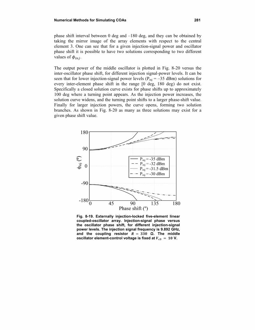
Numerical Me
phase shift intaking the melement 3. Ophase shift itvalues of The output pinter-oscillatoseen that for every inter-eSpecifically a100 deg whesolution curvFinally for lbranches. Asgiven phase s
Fctpao
ethods for Sim
nterval betwemirror image One can see tt is possible
.
power of the or phase shiftlower injecti
element phasea closed soluere a turning ve widens, andlarger injectis shown in Fshift value.
Fig. 8-19. Extcoupled-oscillthe oscillator power levels. Tand the couoscillator elem
mulating COAs
een 0 deg andof the array
that for a givto have two
middle oscift, for differenion-signal powe shift in the
ution curve expoint appear
d the turning on powers, t
Fig. 8-20 as m
ernally injectator array. Iphase shift,
The injection upling resistoment-control v
s
d –180 deg, ay elements w
ven injection-solutions cor
llator is plotnt injection siwer levels (Pe range [0 d
xists for phasers. As the injpoint shifts t
the curve opmany as thre
ion-locked fivnjection-signa
for differentsignal frequen
or voltage is fixed
and they can with respect -signal powerrresponding to
ted in Fig. 8gnal-power leinj = –35 dBm
deg, 180 deg)e shifts up toection power
to a larger phpens, forminge solutions m
ve-element linal phase vert injection-signcy is 9.892 GΩ. The mid
d at
28
be obtained bto the centr
r and oscillato two differe
8-20 versus thevels. It can b
m) solutions f) do not exi
o approximater increases, th
hase-shift valug two solutiomay exist for
near rsus gnal GHz, ddle V.
81
by ral tor ent
the be for ist. ely the ue. on r a

282
Fig. 8oscilshift,signa
fixed
Subsequentlydetermine whThe solutionsimulation, oequations coprevious sectlocked solutian optimum shift range.
8.6 Harm
When an arrmaximum starray elemenphase of 0 ddistributions where the radbeam can bmeasured fro
8-20. Externallator array. M, for differental frequency
Ω. The at V
y, the stabilithich of the mu stability ma
or by examiniorresponding tions. In Ref.ons of a two-coupling stre
monic Rad
ray of oscilltable phase-shnts is 180 deg.deg, this transΔ in the –
diating elemebe scanned aom broadside,
ly injection loiddle oscillatot injection sig
is 9.892 Gmiddle oscil
V.
ty of the soultiple solutioybe determining the eigenvto one of th
. [120], Colla-element arrayength that lea
diation for
lators is couphift range th. In the case oslates to bein–90 deg to 90ents are placeaccording to for a maximu
ocked five-elemor output powgnal power leHz, and thelator element
lutions must ons are stablened using tranvalues of the he analytical ado and Georgy, and it was
ads to a maxim
r Extended
pled at the fhat can be inof a coupling ng able to ge0 deg range.
ed at a half-wΔ si
um of 30
ment linear cower versus theevels. The inje coupling rt control volt
be examinee and will appnsient or envlinear variatimodel formu
giadis studieddetermined tmum stable c
d Scannin
fundamental ntroduced betnetwork that
enerate constConsidering
wavelength disn sin0 deg.
Chapter
oupled-e phase jection
resistor tage is
ed, in order pear in practicvelope-transieional system ulations of td the injectiothat there exisconstant phas
ng Range
frequency, ttween adjacet has a couplintant phase-sh
a linear arrstance, its ma, where
r 8
to ce. ent of
the on-sts se-
the ent ng
hift ray ain
is
Numerical Methods for Simulating COAs 283
It is possible to extend the phase-scanning range by considering the fact that the phase variation of the oscillator Nth harmonic is times the phase variation of its fundamental frequency component, where is the harmonic order. The task of the designer then becomes that of being able to generate sufficient power in the desired harmonic component. Essentially there are two ways of implementing such architectures, either by placing a frequency -tupler circuit at the output of each oscillator, or by properly designing the oscillator elements to have maximum power at the harmonic under consideration. In Ref. [145], Alexanian et.al. proposed a linear array of five coupled oscillators, where each oscillator element is followed by a frequency doubler, as shown in Fig. 8-21. The fundamental frequency of the oscillators is 4 GHz, and their output power is 9 dBm. The prototype array in Ref. [145] used a compact field-effect transistor (FET) based frequency doubler circuit with 1 dB conversion gain. The theoretical phase-tuning range that can be achieved with this topology is 360 deg. Based on the same principle, a frequency tripled two-dimensional coupled-oscillator array operating in X-band was reported by Pogorzelski in Ref. [69]. An inter-oscillator phase difference ranging up to 60 deg was tripled to 180 deg. Thus, this array had a demonstrated H-plane scanning range of ±90 deg. The fabricated prototype additionally contained a diagnostic system used to evaluate the phase differences between the various oscillator elements. The array is described in more detail in Section 6.2. Alternatively, Sanagi et.al. [146] proposed a four-element coupled-oscillator array, where the oscillator elements were specifically designed in order to have a high second-harmonic content, thus also obtaining a 360-deg phase-scanning range. The proposed circuit is shown in (Fig. 8-22). The oscillators are coupled using directional couplers. Termination circuits based on the coupler networks are also attached to the edge elements in order to implement a symmetrical coupling network where all oscillators see approximately the same load. Sanagi et al. [146] extended the coupled oscillator model based on the cubic nonlinearity, which was introduced by York [111], in order to study their proposed circuit architecture. Specifically they considered a nonzero square term in the cubic polynomial describing the current-to-voltage characteristic of the nonlinear device used for the oscillators, and additionally, Sanagi et al. [146] introduced in the formulation an additional equation pertaining to the second harmonic. The block diagram of the considered circuit topology is shown in Fig. 8-23, which was used to investigate the effects in the array performance due to coupling both at the fundamental frequency and at the second harmonic. It was shown that as the
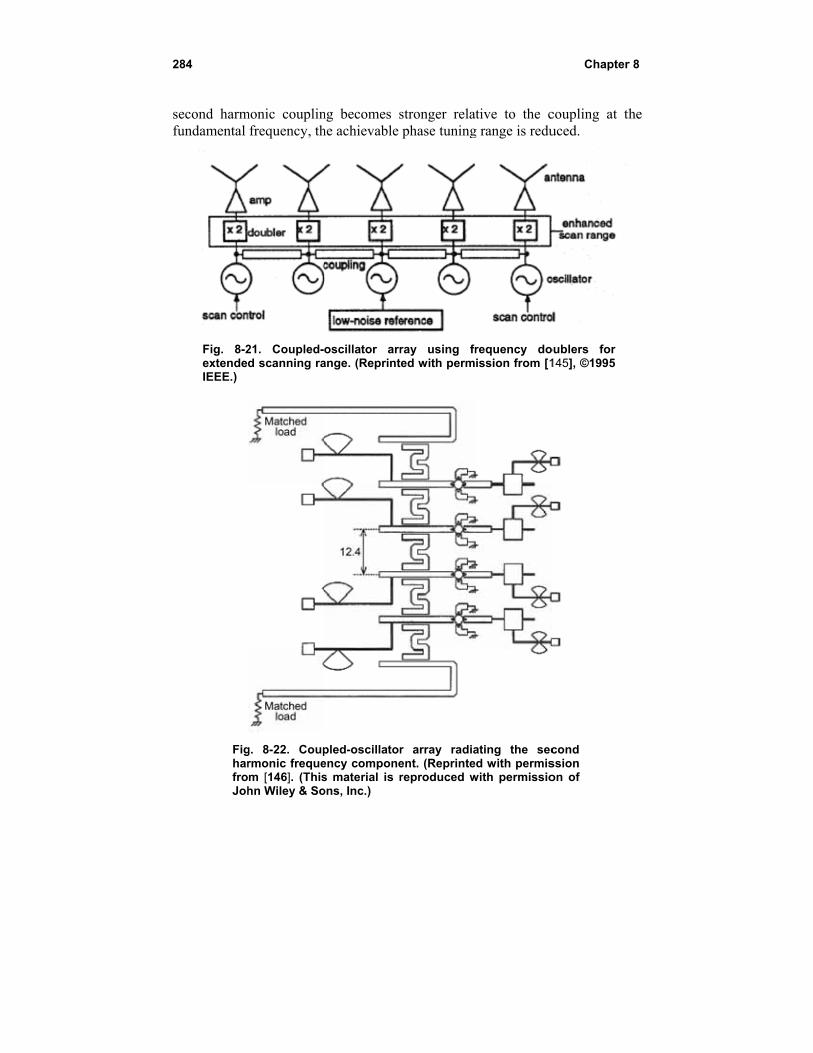
284
second harmfundamental
Fig. 8-2extendeIEEE.)
FigharfroJoh
monic couplinfrequency, th
21. Coupled-d scanning ra
g. 8-22. Couprmonic frequem [146]. (Thishn Wiley & So
ng becomes she achievable
oscillator arrange. (Reprint
pled-oscillatorency compones material is rons, Inc.)
stronger relatphase tuning
ray using frted with perm
r array radiaent. (Reprintereproduced w
tive to the cg range is redu
requency doission from [1
ating the secd with permis
with permissio
Chapter
coupling at tuced.
oublers for 145], ©1995
cond ssion on of
r 8
the
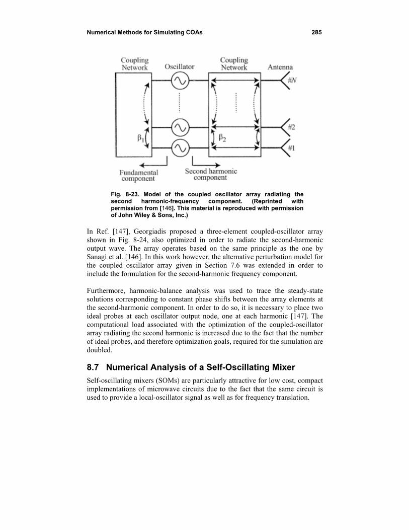
Numerical Me
Fig. secopermof Jo
In Ref. [147shown in Figoutput waveSanagi et al. the coupled include the fo Furthermore,solutions corthe second-hideal probes computationaarray radiatinof ideal probdoubled.
8.7 Num
Self-oscillatinimplementatiused to provi
ethods for Sim
8-23. Model nd harmon
mission from [1ohn Wiley & So
7], Georgiadig. 8-24, also. The array o[146]. In thisoscillator arr
ormulation fo
, harmonic-brresponding toarmonic comat each osci
al load assocng the secondes, and theref
merical Ana
ng mixers (SOions of microide a local-osc
mulating COAs
of the coupic-frequency 146]. This matons, Inc.)
s proposed ao optimized ioperates bases work howevray given in
or the second-
alance analyo constant ph
mponent. In orllator output
ciated with thd harmonic isfore optimizat
alysis of a
OMs) are parowave circuitcillator signal
s
pled oscillatocomponent
terial is reprod
a three-elemein order to raed on the samver, the alternn Section 7.6-harmonic fre
ysis was usedhase shifts berder to do so,node, one at
he optimizatioincreased duetion goals, req
a Self-Osc
rticularly attras due to the l as well as fo
r array radiat. (Reprinteduced with pe
ent coupled-oadiate the seme principle ative perturba was extendquency comp
d to trace thetween the arr
it is necessart each harmoon of the coue to the fact tquired for the
cillating M
active for lowfact that the
or frequency t
28
ating the ed with ermission
oscillator arrecond-harmon
as the one bation model f
ded in order ponent.
he steady-staray elements
ary to place twonic [147]. Thupled-oscillatthat the numbe simulation a
Mixer
w cost, compasame circuit
translation.
85
ray nic by for to
ate at
wo he tor ber are
act is
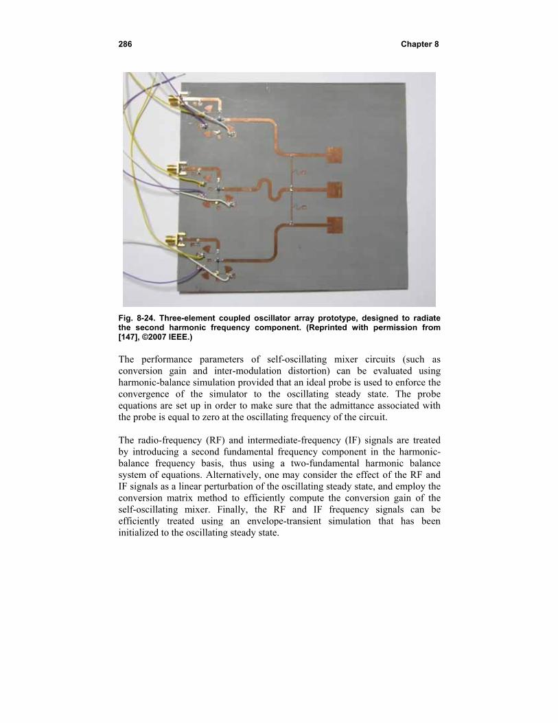
286
Fig. 8-24. Thrthe second h[147], ©2007 I The performconversion gharmonic-balconvergence equations arethe probe is e The radio-freby introducinbalance freqsystem of eqIF signals as conversion mself-oscillatinefficiently trinitialized to
ree-element charmonic freqIEEE.)
mance paramgain and intlance simulat
of the sime set up in orequal to zero
equency (RF)ng a second
quency basis,quations. Alte
a linear pertumatrix methong mixer. Freated usingthe oscillatin
coupled oscillquency comp
meters of seter-modulatiotion provided
mulator to thrder to make at the oscillat
) and intermefundamental , thus using
ernatively, onurbation of thd to efficieninally, the R
g an envelopng steady state
ator array proponent. (Repr
elf-oscillatingon distortionthat an ideal
he oscillatingsure that the
ting frequency
ediate-frequenfrequency ca two-fund
ne may conside oscillating stly compute RF and IF pe-transient e.
ototype, desigrinted with pe
mixer circ) can be evprobe is used
g steady stat admittance ay of the circu
ncy (IF) signomponent in
damental harmder the effectsteady state, athe conversifrequency ssimulation t
Chapter
gned to radiaermission fro
cuits (such valuated usind to enforce t
ate. The probassociated wi
uit.
nals are treatthe harmoni
monic balant of the RF anand employ thion gain of tsignals can bthat has be
r 8
ate om
as ng the be ith
ted ic-
nce nd the the be en
Numerical Methods for Simulating COAs 287
In Ref. [148], Herran et al. optimized the gain associated with a selected mixing product of a self-oscillating mixer by using two ideal probes properly introduced in the circuit and optimizing the reflection coefficients of an ideal multi-harmonic load connected to the circuit input. The circuit schematic that was used is shown in Fig. 8-25. The first probe, called an auxiliary generator in Fig. 8-25, is used to enforce the oscillation condition at the desired frequency. The admittance looking into this probe is set to zero in order not to perturb the circuit steady state, and the complex admittance or reflection coefficient of the multi-harmonic load at the fundamental frequency that satisfies this condition is found through harmonic balance optimization. The second ideal generator probe is connected in series with the gate terminal of the FET device, and its frequency corresponds to a desired th harmonic that is selected for the mixing process. Mixing products involving the second and third harmonics were considered. The reflection coefficient of the multi-harmonic load at the desired harmonic is set to –1, corresponding to a short circuit. The optimization procedure consists of finding the complex amplitude of the ideal generator which results in a desired mixing gain value. The corresponding admittance looking into the generator must have a positive real part in order for it to correspond to a passive load. In this way, the multi-harmonic load is optimized for a desired mixing gain value and its reflection coefficient at the fundamental frequency and selected harmonic frequency are determined. The final design is obtained by implementing the obtained reflection coefficient values using passive printed or lumped circuit components [148]. A varactor diode may be appropriately placed in the self-oscillating mixer circuit in order to provide a frequency-tuning capability. An externally injection-locked self-oscillating mixer operates both as a mixer and a phase-shifter element, where the phase shift between the input and output of the mixer is varied by changing the free-running frequency of the self-oscillating mixer. Being a synchronized oscillator, the externally injection locked self-oscillating mixer can be used to provide a continuous phase-shift range of N × 180 deg where the external injection signal is assumed to have a frequency near the fundamental frequency of oscillation of the self-oscillating mixer, and the th oscillator harmonic is used in the mixing operation. Here, the fact that the tuning range of the phase of the oscillator th harmonic is times the tuning range of the phase of its fundamental frequency component being used [145].

288
Fig. 8-25. Noninput signal o
, before it intermediate consists of dOptimization amplitude generator witmulti-harmonreflection coe
. (c) Impfor the casesmixer, respec It has been externally injto transmit in
nlinear optimiof power is mixed by frequency filt
designing a mis performe and frequen
th amplitude nic load usingefficients
plementation os of a secondctively. (Reprin
argued in Sjection lockednformation b
zation of a sepasses throuthe active cirter of center
multi-harmoniced using an ncy defin
at the harg ideal circuit correspondinof the multi-hd (2 HSOM) anted with perm
Sections 7.9d oscillator a
by introducing
elf-oscillating ugh a band-parcuit and colle
frequency c load with im
ideal auxilianed as in Figrmonic frequecomponents.g to the load
harmonic loadnd third (3 H
mission from [
and 8.5 dearrays that sucg phase or fr
mixer. (a) Circass filter withected at the o
. The optimmpedance ary generator. 8.2, as well ency . (b). The figure ind impedance d using microSOM) harmon[148], ©2006 IE
aling with thch architecturrequency mo
Chapter
cuit topology:h center frequoutput throug
mization proceat harmonic
r probe AG as a substitu
) Definition ondicates the i at frequ
ostrip componnic self-oscillaEEE.)
he analysis res can be us
odulation in t
r 8
: The
uency gh anedure
. with
ution of the input
uency nents ating
of ed
the
Numerical Methods for Simulating COAs 289
external injection signal. Furthermore, the effect of modulation in the array scanning range was investigated in Section 7.11. Such topologies are limited to relatively narrowband applications due to the fact that the modulation strongly affects the steady state of the synchronized oscillator signals. Furthermore, specific modulation formats leading to small envelope variations are suitable for such applications due to the fact that the amplitude-limiting properties of the oscillators tend to introduce distortion to the envelope of the modulating signals. Continuous phase modulation (CPM) [149], which is a constant envelope modulation, is a prominent candidate for such systems. A well known example of CPM is Gaussian minimum-shift keying (GMSK) used in the Global System for Mobile Communications (GSM), second-generation mobile (cellular) communication systems. However, when modulation is introduced through the RF input signal of the self-oscillating mixer, it does not strongly affect the synchronization state of the mixer due to the fact that the input signal has a low power level and represents only a perturbation of the steady state. As a result, self-oscillating mixers can be used as frequency translation and phase-shifter circuits for input RF signals of arbitrary modulation. Furthermore, proper design of the mixer can allow one to obtain broadband gain and therefore the self-oscillating mixer is not limited to RF input signals with narrowband modulation. The use of an injection-locked self-oscillating mixer as a downconverter and phase shifter element was studied by ver Hoeye [80]. The proposed circuit topology is the same as in Fig. 8-25 with the addition of a varactor diode connected in parallel with the series feedback shorted stub present at the source terminal of the active device in order to provide a frequency tuning capability. The SOM design was performed using the methodology described previously in this section. An oscillation at 3.25 GHz was obtained, and an RF signal of 11.25 GHz was mixed with the third harmonic of the SOM, resulting in an IF output of 1.5 GHz. Phase tuning of as much as 3 × 180 deg = 540 deg was achieved by utilizing the third harmonic mixing product. The obtained conversion gain was 4.5 dB over a bandwidth of approximately 100 MHz. It is shown in Fig. 8-26 that the conversion gain depends both on the injection power level Ps and on the varactor control voltage Vcont or, in other words, the selected phase difference between the input and output SOM terminals. The results have been obtained using a two-fundamental-harmonic balance simulation, and one can observe the closed synchronization curves of the injection locked self-oscillating mixer, which are similar to the ones obtained for the synchronized oscillator in Fig. 8-7. The synchronization curves open as the injection power increases, and there exist two solutions for a given control voltage within the synchronization band limited by the curve edges of infinite slope. Only one of the two solutions is stable and therefore measured
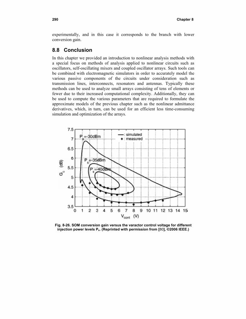
290
experimentalconversion g
8.8 Conc
In this chaptea special focoscillators, sebe combinedvarious passtransmission methods can fewer due tobe used to capproximate derivatives, wsimulation an
Fig. 8-26. SOinjection p
lly, and in tain.
clusion
er we providecus on methoelf-oscillating
d with electrosive compon
lines, intercbe used to a
their increasompute the vmodels of th
which, in turnd optimizatio
OM conversiopower levels P
this case it
ed an introduods of analysg mixers and magnetic sim
nents of the connects, resanalyze small sed computativarious paramhe previous crn, can be uson of the arra
n gain versusPs. (Reprinted w
corresponds
uction to nonlsis applied tocoupled osci
mulators in orcircuits un
sonators and arrays consi
ional complemeters that archapter such sed for an effays.
s the varactor with permissio
to the branc
inear analysiso nonlinear cllator arrays. rder to accurader consider
antennas. Tsting of tens
exity. Additiore required toas the nonlin
fficient less ti
control voltagon from [80], ©
Chapter
ch with low
s methods wicircuits such
Such tools cately model thration such Typically the
of elements onally, they co formulate thnear admittanime-consumin
ge for differen©2006 IEEE.)
r 8
wer
ith as an
the as
ese or an
the nce ng
nt
291
Chapter 9 Beamforming in Coupled-Oscillator
Arrays
In this chapter, convex optimization and other global optimization techniques are used to demonstrate the beamforming capabilities of coupled-oscillator arrays and to optimize the stability of the coupled-oscillator array steady-state solution. An introduction to convex optimization is presented followed by several optimization problems showing the beamforming capabilities of such arrays, such as pattern-nulling, difference-beam generation, and multiple-beam generation [96,118,150,151,152]. A global optimization algorithm is also presented that permits one to optimize the stability of the steady-state solution, and therefore leads to more robust solutions and maximizes the obtained stable beam-scanning limits [153]. Finally, the operation of a coupled-oscillator array as an adaptive beamforming system is demonstrated [154].
9.1 Preliminary Concepts of Convex Optimization
Convex optimization is a class of optimization problems that has enjoyed an increased scientific interest in the recent years due to the development of very efficient algorithms essentially rendering their solution as easy as the solution of linear programs [133]. As a result convex optimization problems have found wide application in fields such as control and signal processing, and among these, in the problem of antenna array beam-steering and beamforming. Due to this fact, in this chapter we first present a brief introduction to convex optimization and the mathematical framework required to express the beamforming problem as a convex optimization problem and additionally
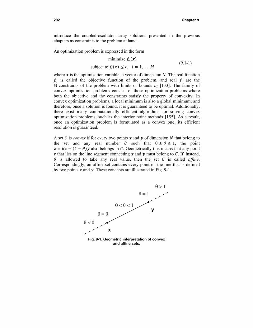
292
introduce thchapters as co An optimizat
where is th is calledconstraints
convex optimboth the objconvex optimtherefore, onthere exist moptimization once an optresolution is A set is cothe set an
1 that lies on is allowe
Correspondinby two points
he coupled-osonstraints to t
tion problem
subjec
he optimizatiothe objecti
s of the probmization probjective and th
mization probce a solution many compuproblems, su
imization proguaranteed.
nvex if for evnd any real
also bn the line segmed to take angly, an affins and . Th
Fig. 9-1
scillator arrathe problem a
is expressed i
minimize
ct to
on variable, a ve function blem with limblems consisthe constraintlems, a local is found, it i
utationally efuch as the inoblem is for
very two poinl number belongs in . ment connectiany real val
ne set containhese concepts
. Geometric inand aff
ay solutions at hand.
in the form
e
1, . . .
vector of dimof the prob
mits or bounts of those opts satisfy theminimum is s guaranteed fficient algor
nterior point mrmulated as a
nts and of such tha
Geometricaling and mlue, then th
ns every poinare illustrated
nterpretation ofine sets.
presented in
,
mension . Thblem, and reds [133].ptimization pe property ofalso a global to be optimarithms for smethods [155a convex on
f dimension at 0ly this means
must belong tohe set is nt on the line d in Fig. 9-1.
of convex
Chapter
n the previo
(9.1-1)
he real functioeal are thThe family
problems whef convexity. minimum; an
al. Additionallsolving conv5]. As a resune, its efficie
that belong 1, the poi
s that any poio . If, instea
called affinthat is defin
r 9
ous
on the of
ere In nd ly,
vex ult, ent
to int int ad, ne. ed
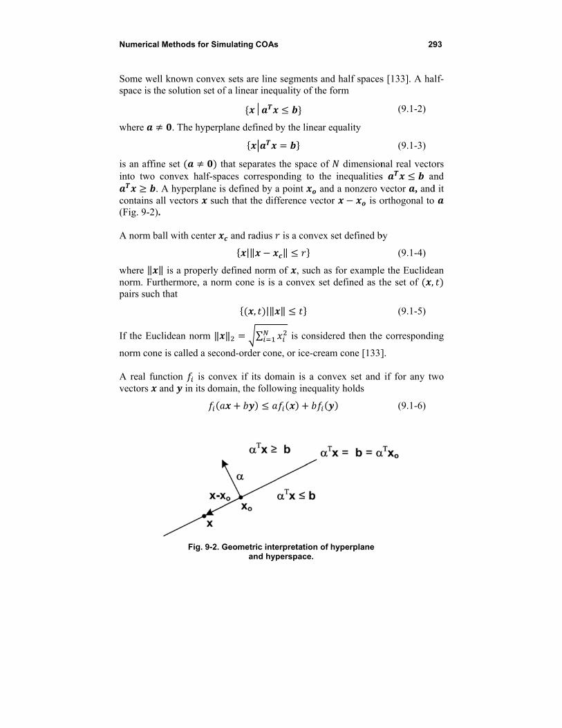
Numerical Me
Some well knspace is the s
where
is an affine sinto two con
. A contains all v(Fig. 9-2). A norm ball w
where ‖ ‖ isnorm. Furthepairs such tha
If the Euclid
norm cone is A real functivectors and
ethods for Sim
nown convexsolution set of
. The hyperpl
set thnvex half-spahyperplane isvectors suc
with center
s a properly dermore, a norat
dean norm ‖
called a seco
ion is convd in its dom
Fig. 9-2. G
mulating COAs
x sets are linef a linear ineq
lane defined b
hat separates aces correspos defined by ah that the dif
and radius
|‖
defined norm rm cone is is
, |‖
‖ ∑
ond-order con
vex if its dommain, the follo
Geometric inteand hyp
s
e segments anquality of the
by the linear e
the space of onding to thea point anfference vecto
is a convex
‖
of , such asa convex set
‖
is conside
ne, or ice-crea
main is a conwing inequal
erpretation of perspace.
nd half spacesform
equality
f dimensione inequalities
nd a nonzero vor is o
set defined b
s for examplet defined as t
ered then the
am cone [133]
nvex set and ity holds
hyperplane
29
s [133]. A ha
(9.1-2)
(9.1-3)
nal real vectos anvector , andorthogonal to
by
(9.1-4)
e the Euclidethe set of ,
(9.1-5)
e correspondin
].
if for any tw
(9.1-6)
93
alf-
ors nd
d it
an
ng
wo
294 Chapter 9
where and are non-negative real numbers such that 1. One can easily verify from Eq. (9.1-6) that a linear function is convex. Another commonly used convex constraint is a linear matrix inequality [156]
∑ 0 (9.1-7)
where is a vector of dimension and are real symmetric matrices of dimension . A real square matrix is positive definite
0, if for any nonzero vector , 0. Many convex constraints such as linear inequalities, convex quadratic inequalities, and Lyapunov matrix inequalities can be cast in the form of a linear matrix inequality. According to Lyapunov theory, the system of differential equations
(9.1-8)
is stable if and only if exists a positive definite matrix such that
0 (9.1-9)
The above inequality is known as a Lyapunov matrix inequality. The inequality of Eq. (9.1-9) with the matrix as unknown can be cast in the form of a linear matrix inequality [156]. The minimization of the maximum eigenvalue of a matrix subject to a linear matrix inequality constraint 0 is a convex problem defined as [156]
minimize λ
subject to , (9.1-10)
with and symmetric matrices that depend affinely on . If one defines an extended unknown vector and 1 the eigenvalue minimization problem can be written as minimization of a linear function subject to a linear matrix inequality
minimize
subject to (9.1-11)
where together with have been formulated as a single linear matrix inequality . Linear programming and least-squares optimization are two well known examples of convex optimization problems. In linear programming, both the objective and the constraints are linear functions
minimize
subject to 1, . . . , (9.1-12)
Numerical Methods for Simulating COAs 295
In least squares optimization the objective function is a sum of squares which is a convex function and there are no constraints
minimize ‖ ‖ ∑ (9.1-13)
Where is an M by N matrix, ai is a vector of dimension N containing the elements of column i of matrix A, and b is a vector of dimension M. Finally, the minimization of the maximum generalized eigenvalue of a pair of symmetric matrices and that depend affinely on , subject to an additional linear matrix inequality constraint 0 is a quasi-convex optimization problem [156] expressed as
minimize λ
subject to , , (9.1-14)
A real function is quasi-convex if and only if its domain is a convex set, and for any two vectors and in its domain, and a real number , such that 0 1, the following inequality holds [133]
1 max , (9.1-15)
Convex functions are also quasi-convex but not vice-versa. The standard formulation of a quasi-convex optimization problem has a quasi-convex objective and convex constraints. The generalized eigenvalue minimization problem given by Eq. (9.1-14) can be written in the standard format [156,133]. Similarly to convex optimization problems, quasi-convex optimization problems can also be solved efficiently.
9.2 Beamfoming in COAs
The ability to generate constant phase distributions among the coupled-oscillator array elements by tuning the frequency of only the edge array elements has been one of the most attractive properties of coupled-oscillator arrays as they can be used in beam-scanning applications eliminating the need for phase shifters or a complicated local-oscillator feed network. If, however, one is allowed to tune the frequency of more or all the array elements, then additional features maybe introduced in the radiated pattern such as placement of nulls at desired far-field angular directions. Once a constant progressive phase shift is established among the array elements, the main beam direction is steered towards a desired direction. In Ref. [157], Steyskal showed that additional nulls maybe formed in the radiation pattern at desired angular directions by introducing small perturbations to the

296 Chapter 9
phases of the array elements. This method was used by Heath [96] in conjunction with the generalized phase model to demonstrate beamforming capabilities using coupled-oscillator arrays. Finally, Georgiadis et al. [118] extended Heath’s work by including both amplitude and phase perturbations. In the following, a description of this beamforming methodology is provided. The array factor of a uniform linear antenna-array of elements is given by
∑ (9.2-1)
where the element distance is , and the angular direction is measured from broadside. The main beam is steered at when the excitation amplitudes are equal and the element phases are set as sin . The array factor is then written in compact form
(9.2-2)
where . If one introduces a perturbation in the excitation amplitudes and phases the array factor is approximated to first order as
(9.2-3)
A constraint in the array factor at angle is introduced by imposing | | where is a desired maximum level at . Given level constraints,
one may form a complex vector … containing all the constraints and a second one containing … and combine them in a matrix inequality
(9.2-4)
which can be written in compact form
(9.2-5)
The beamforming problem can be formulated as a convex optimization problem as follows
min
subject to ‖ ‖
(9.2-6)
where the linear objective is subject to a second-order cone constraint and a linear inequality. Minimizing the norm of ensures that the perturbation approximation of the array factor is valid.

Numerical Methods for Simulating COAs 297
The problem given by Eq. (9.2-6) was analytically solved by Georgiadis et al. in Ref. [118] for the case where the inequality constraints are null constraints
. In fact, the analytical solution to this problem when considering phase perturbations only was given by [157]. In this case [157,118],
(9.2-7)
and
∆ (9.2-8)
It is interesting to study Eq. (9.2-7), for the simple case of main-beam direction at with one nulling constraint at angle . One then evaluates as
∑ cos∑ sin
(9.2-9)
where sin sin . This shows that there exist combinations of and such that the required perturbation magnitude goes to infinity, for which
the optimization problem does not have a solution. These solutions correspond to where and are integers. One such solution is for 0, which corresponds to ; or in other words, when the desired null is in the direction of the main lobe. A second solution is when
sin sin (9.2-10)
which corresponds to a desired null direction that depends on the main beam angle . The existence of such points was also verified numerically for the case of a coupled-oscillator array in [118,150]. In order to apply the pattern constraints to the coupled oscillator array, one needs to limit the perturbation vectors satisfying Eq. (9.2-6) to the set that corresponds to a coupled-oscillator array steady-state solution. Reference [118] introduced the coupled-oscillator array steady-state solution in Eq. (9.2-6) as an additional linear constraint maintaining the convexity of the optimization problem. The steady-state solution (7.7-12) is first reformulated to reflect the nature of perturbation , which contains both amplitude ∆ and phase perturbations ∆ sin ∆ . Due to the autonomous nature of the coupled oscillator array, the steady-state solution is defined by the relative phases of the oscillator elements. In other words, the phase of one oscillator maybe set to an arbitrary value, or alternatively the phases of all oscillators can be changed by an equal amount without affecting the steady state. This is verified by the steady-state expression Eq. (7.6-10) where only phase differences are present. Consequently, a perturbation of the steady state is set by considering the terms ∆ such that even though
298 Chapter 9
individually they may take large values, their relative differences are kept small. This argument was also used in the early works of Kurokawa [105] when modeling the externally injection-locked oscillator. It is, therefore, possible to approximate the phase exponents appearing in Eq. (7.6-10) as
1 ∆ ∆
and obtain the perturbed steady state as
∆
0 (9.2-11)
with
dg (9.2-12)
The final system of equations is obtained by separating real and imaginary parts
∆
(9.2-13)
which is written in compact form
∆ (9.2-14)
Using the above linear constraint for the steady state, it is possible to formulate the beamforming optimization problem for coupled oscillator arrays [118] as follows
min,
subject to ‖ ‖ ‖ ‖
∆
(9.2-15)
where the norm of the vector is also minimized in order to enforce the perturbation condition pertaining to the derivation of the steady-state constraint. The above formulation was extended to planar arrays in Ref. [150].
Numerical Methods for Simulating COAs 299
Once the steady state is obtained, its stability is examined by considering the linear variational system corresponding to the system of differential equations describing the coupled oscillator dynamics and evaluating the eigenvalues of matrix or in Eq. (7.7-17). We may further explore the arbitrary phase reference of the coupled oscillator array in order to minimize the number of optimization variables in Eq. (9.2-15).
is a square matrix of dimension 2 . It has one zero eigenvalue due to the fact that the array steady state is unaffected by applying an arbitrary but constant phase term to all elements. It is therefore possible, without loss of generality, to set the phase perturbation of an arbitrarily selected element to zero ∆ 0 and eliminate the column of that corresponds to ∆ . Then, a new steady-
state vector Δ of dimension 2 is constructed, where contains all phase perturbations except ∆ . Using , Eq. (9.2-14) is
rearranged in the form
∆ ∆ ⇒ ∆ (9.2-16)
where Δ is the control perturbation corresponding to the selected element . is a full rank square matrix of dimension 2 obtained from by substituting its column corresponding to ∆ with the column of ∆ corresponding to Δ . Similarly ∆ , has dimension 2 by 1 and is obtained from ∆ by eliminating the column that corresponds to Δ . The matrix ∆ is linearly dependent on ∆ . The steady state is therefore expressed as a function of the
1 independent control variables ∆ . Following Georgiadis et al. [153], the equality constraint of Eq. (9.2-16) is used to eliminate the 2 optimization variables included in , and formulate Eq. (9.2-15) in terms of only the independent 1 control variables ∆
min∆
subject to ∆ ‖∆ ‖
∆ ∆ ∆ ∆
(9.2-17)
where the equality constraint is now eliminated and the inequality constraints on the array factor have been appropriately reformulated in terms of the independent control variables. As an example, let us consider the five-element coupled oscillator array of Section 8.4, assuming that each oscillator output is connected to an antenna, and the antenna elements are placed a half free-space wavelength apart . The free-running oscillator steady state corresponds to an amplitude of 0.442 V (the output power is 2.9 dBm), and frequency 9.892 GHz obtained for a control voltage of 10 V.
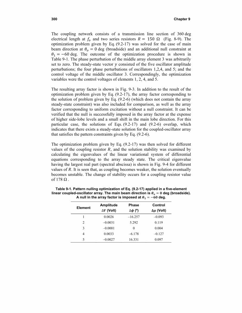
300 Chapter 9
The coupling network consists of a transmission line section of 360 deg electrical length at and two series resistors 150 Ω (Fig. 8-9). The optimization problem given by Eq. (9.2-17) was solved for the case of main beam direction at 0 deg (broadside) and an additional null constraint at
60 deg. The outcome of the optimization procedure is shown in Table 9-1. The phase perturbation of the middle array element 3 was arbitrarily set to zero. The steady-state vector consisted of the five oscillator amplitude perturbations; the four phase perturbations of oscillators 1,2,4, and 5; and the control voltage of the middle oscillator 3. Correspondingly, the optimization variables were the control voltages of elements 1, 2, 4, and 5. The resulting array factor is shown in Fig. 9-3. In addition to the result of the optimization problem given by Eq. (9.2-17), the array factor corresponding to the solution of problem given by Eq. (9.2-6) (which does not contain the array steady-state constraint) was also included for comparison, as well as the array factor corresponding to uniform excitation without a null constraint. It can be verified that the null is successfully imposed in the array factor at the expense of higher side-lobe levels and a small shift in the main lobe direction. For this particular case, the solutions of Eqs. (9.2-17) and (9.2-6) overlap, which indicates that there exists a steady-state solution for the coupled-oscillator array that satisfies the pattern constraints given by Eq. (9.2-6). The optimization problem given by Eq. (9.2-17) was then solved for different values of the coupling resistor , and the solution stability was examined by calculating the eigenvalues of the linear variational system of differential equations corresponding to the array steady state. The critical eigenvalue having the largest real part (spectral abscissa) is shown in Fig. 9-4 for different values of . It is seen that, as coupling becomes weaker, the solution eventually becomes unstable. The change of stability occurs for a coupling resistor value of 178 Ω .
Table 9-1. Pattern nulling optimization of Eq. (9.2-17) applied in a five-element linear coupled-oscillator array. The main beam direction is deg (broadside).
A null in the array factor is imposed at deg.
Element Amplitude
∆ (Volt)
Phase
∆ (º)
Control
(Volt)
1 0.0026 –16.257 –0.093
2 –0.0031 5.292 0.119
3 –0.0001 0 0.004
4 0.0033 –6.178 –0.127
5 –0.0027 16.331 0.097

Numerical Me
Faf
ethods for Sim
Fig. 9-3. Beamarrays. Array for main beam
deg.
Fig. 9-4. Croptimizationcoupling res
mulating COAs
mforming capfactor of five
m at broadsid The coupling
ritical eigenvan problem osistor .
s
pabilities of coe-element arrade and one ng resistor is
alue of the sof Eq. (9.2-17
oupled oscillaay of Section null constrain
Ω.
solution of th7) versus th
30
ator 8.4
t at
he he
01

302 Chapter 9
9.3 Stability Optimization of the Coupled-Oscillator Steady-State Solution
The stability of the coupled oscillator steady-state solution is verified by examining the linear variational equations corresponding to the system of nonlinear differential equations describing its dynamics. In Section 7.7, a procedure was described to remove the zero eigenvalue that appears due to the free-running nature of the oscillator array. The resulting square matrix of dimension 2 1 was derived in Section 7.7, where is the size of the array. The linear variational equation for is repeated here for convenience, where contains 1 phase differences with respect to an arbitrarily selected oscillator as a reference
(9.3-1)
By definition, a steady-state solution is stable if the spectral abscissa of is negative. The decay rate of is the negative of the spectral abscissa [156], and a steady state is stable if has a positive decay rate. Maximizing the decay rate corresponds to a more robust steady-state solution, less likely to lose its stability due to the presence of noise or other perturbations. The matrix ∆ ) depends on the steady state defined by the perturbation vector
of the array, which, following Eq. (9.2-16), is determined by the (perturbation) vector of 1 control voltages ∆ . does not depend linearly on ∆ due to the matrix inversion involved in its derivation and due to the fact that the phase terms appear in exponential terms. This can be easily verified following the formulation that leads to the definition of in Section 7.7. However, due to the fundamental assumption that and ∆ are small, we may consider the first order expansion ∆ ) of ∆ ). The derivation of ∆ ) is straightforward. A lower bound on the decay rate can be obtained using Lyapunov theory as the maximum that solves [156]
2 (9.3-2)
for any , where is a scalar quadratic potential function defined by a 0real symmetrix matrix with dimension 2 1 such that
(9.3-3)
Using Eqs. (9.3-1) and (9.3-3) in Eq. (9.3-2), one obtains a matrix inequality
2 0 (9.3-4)
For a given steady state ∆ , finding the symmetric positive definite matrix that maximizes the decay rate is a generalized eigenvalue optimization
Numerical Methods for Simulating COAs 303
problem. Conversely, given a specific matrix finding the steady state ∆ that maximizes is an eigenvalue optimization problem. As noted in Section 9.1, both such problems can be efficiently solved using convex optimization algorithms. However, finding the steady state ∆ and matrix that maximize is not a convex optimization problem due to the multiplicative terms that appear between the elements of ∆ and . It is possible to introduce the decay-rate optimization constraint in the coupled-oscillator array beamforming optimization algorithm following the approach by Georgiadis and Slavakis [153], which is given below. The optimization problem including the stability constraint is written as follows
, min∆ ,
subject to (i) ∆ ‖∆ ‖
(ii) ∆ ∆ ∆
(iii) ∆ ∆ 2
(iv) 0
(9.3-5)
This is not a convex optimization problem, and its resolution is not straightforward. In Ref. [153], an algorithm was proposed to obtain a solution to the above problem by alternative minimization of two sub-problems, an eigenvalue and a generalized eigenvalue problem. The algorithm proceeds as follows Step 1: Let 0 be the algorithm termination tolerance and 0 be the
iteration number. Find ∆ ∆ , the vector of control variables that minimizes the perturbation vector norm , subject to (i) and (ii). This is the original convex optimization problem of Eqs. (9.2-17) and (9.2-15) that does not include a stability constraint. Obtain the decay rate corresponding to ∆ by evaluating its eigenvalues.
Step 2: Repeat
P1: Find the real symmetric square matrix that minimizes 0, , subject to (iii) and (iv) for a given ∆ . This is a
generalized eigenvalue optimization problem. The optimization objective provides a value of the decay rate , .
P2: Find the control vector ∆ that minimizes , using as input the matrix obtained from the previous step. This is an eigenvalue optimization problem. Additional outputs of this step are the norm of the perturbation vector and the decay rate , .
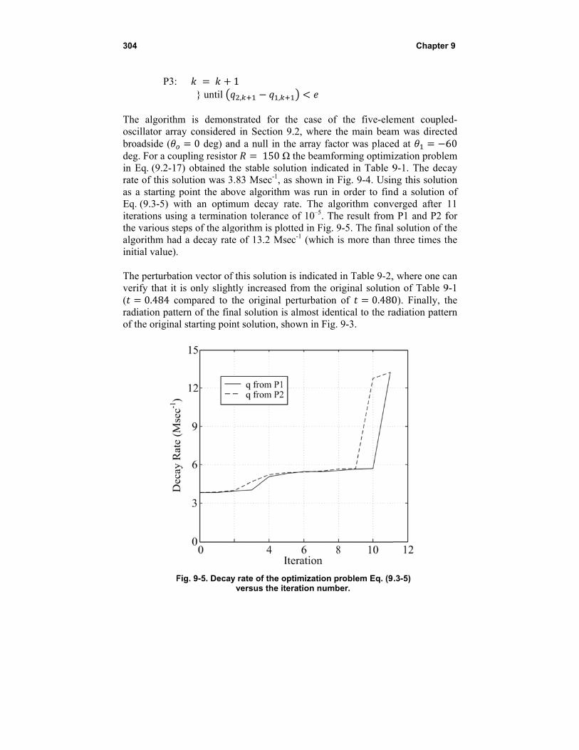
304
P3: The algorithoscillator arrbroadside (deg. For a coin Eq. (9.2-1rate of this soas a starting Eq. (9.3-5) witerations usithe various stalgorithm hainitial value)
The perturbaverify that it ( 0.484 cradiation pattof the origina
until
hm is demonray considere
0 deg) anoupling resisto7) obtained tolution was 3point the ab
with an optiming a terminateps of the algd a decay rat.
tion vector ofis only sligh
compared to tern of the final starting poi
Fig. 9-5. Deca
1
, ,
nstrated for d in Section nd a null in tor 150 Ωthe stable sol3.83 Msec-1, aove algorithm
mum decay ration tolerancegorithm is plote of 13.2 Ms
f this solutionhtly increasedthe original
nal solution isint solution, s
y rate of the oversus the it
the case of 9.2, where th
the array factΩ the beamfolution indicatas shown in Fm was run inrate. The alge of 10–5. Thotted in Fig. 9sec-1 (which i
n is indicated d from the orperturbation s almost idenhown in Fig.
optimization pteration numb
the five-elehe main beamtor was placerming optimi
ted in Table 9Fig. 9-4. Usin
n order to fingorithm conve result from9-5. The finalis more than
in Table 9-2,iginal solutioof 0.480
ntical to the ra9-3.
roblem Eq. (9ber.
Chapter
ement couplem was directed at 6ization proble9-1. The decng this solutio
nd a solution verged after
m P1 and P2 fl solution of ththree times th
, where one con of Table 90). Finally, thadiation patte
.3-5)
r 9
ed-ted 60 em ay on of 11 for the the
an 9-1 the ern
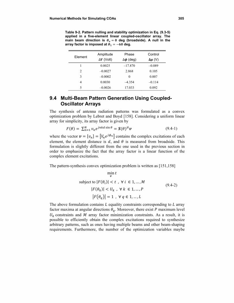
Numerical Methods for Simulating COAs 305
Table 9-2. Pattern nulling and stability optimization in Eq. (9.3-5) applied in a five-element linear coupled-oscillator array. The main beam direction is deg (broadside). A null in the array factor is imposed at deg.
Element Amplitude
∆ (Volt)
Phase
∆ (deg)
Control
(V)
1 0.0025 –17.870 –0.089
2 –0.0027 2.868 0.105
3 –0.0002 0 0.007
4 0.0030 –4.354 –0.114
5 –0.0026 17.033 0.092
9.4 Multi-Beam Pattern Generation Using Coupled-Oscillator Arrays
The synthesis of antenna radiation patterns was formulated as a convex optimization problem by Lebret and Boyd [158]. Considering a uniform linear array for simplicity, its array factor is given by
∑ (9.4-1)
where the vector contains the complex excitations of each element, the element distance is , and is measured from broadside. This formulation is slightly different from the one used in the previous section in order to emphasize the fact that the array factor is a linear function of the complex element excitations. The pattern-synthesis convex optimization problem is written as [151,158]
min
subject to | | , ∀ ∈ 1, … ,
| | , ∀ ∈ 1, … ,
1 , ∀ ∈ 1,… ,
(9.4-2)
The above formulation contains equality constraints corresponding to array factor maxima at angular directions . Moreover, there exist maximum level constraints and array factor minimization constraints. As a result, it is
possible to efficiently obtain the complex excitations required to synthesize arbitrary patterns, such as ones having multiple beams and other beam-shaping requirements. Furthermore, the number of the optimization variables maybe
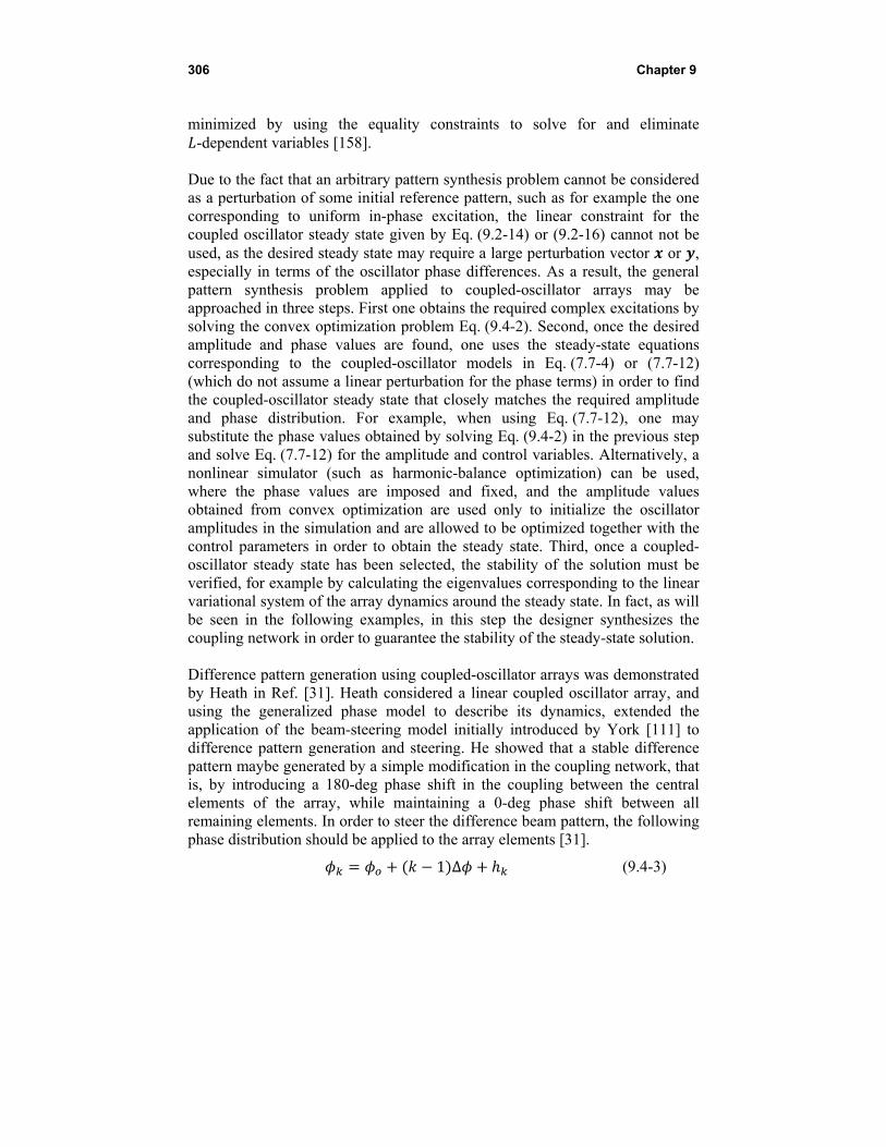
306 Chapter 9
minimized by using the equality constraints to solve for and eliminate -dependent variables [158].
Due to the fact that an arbitrary pattern synthesis problem cannot be considered as a perturbation of some initial reference pattern, such as for example the one corresponding to uniform in-phase excitation, the linear constraint for the coupled oscillator steady state given by Eq. (9.2-14) or (9.2-16) cannot not be used, as the desired steady state may require a large perturbation vector or , especially in terms of the oscillator phase differences. As a result, the general pattern synthesis problem applied to coupled-oscillator arrays may be approached in three steps. First one obtains the required complex excitations by solving the convex optimization problem Eq. (9.4-2). Second, once the desired amplitude and phase values are found, one uses the steady-state equations corresponding to the coupled-oscillator models in Eq. (7.7-4) or (7.7-12) (which do not assume a linear perturbation for the phase terms) in order to find the coupled-oscillator steady state that closely matches the required amplitude and phase distribution. For example, when using Eq. (7.7-12), one may substitute the phase values obtained by solving Eq. (9.4-2) in the previous step and solve Eq. (7.7-12) for the amplitude and control variables. Alternatively, a nonlinear simulator (such as harmonic-balance optimization) can be used, where the phase values are imposed and fixed, and the amplitude values obtained from convex optimization are used only to initialize the oscillator amplitudes in the simulation and are allowed to be optimized together with the control parameters in order to obtain the steady state. Third, once a coupled-oscillator steady state has been selected, the stability of the solution must be verified, for example by calculating the eigenvalues corresponding to the linear variational system of the array dynamics around the steady state. In fact, as will be seen in the following examples, in this step the designer synthesizes the coupling network in order to guarantee the stability of the steady-state solution. Difference pattern generation using coupled-oscillator arrays was demonstrated by Heath in Ref. [31]. Heath considered a linear coupled oscillator array, and using the generalized phase model to describe its dynamics, extended the application of the beam-steering model initially introduced by York [111] to difference pattern generation and steering. He showed that a stable difference pattern maybe generated by a simple modification in the coupling network, that is, by introducing a 180-deg phase shift in the coupling between the central elements of the array, while maintaining a 0-deg phase shift between all remaining elements. In order to steer the difference beam pattern, the following phase distribution should be applied to the array elements [31].
1 Δ (9.4-3)
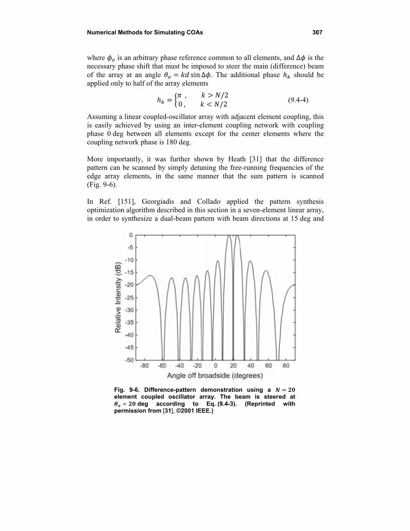
Numerical Me
where is anecessary phof the array applied only
Assuming a lis easily achphase 0 degcoupling netw More importpattern can bedge array e(Fig. 9-6). In Ref. [15optimization in order to sy
Fig. elem
perm
ethods for Sim
an arbitrary phase shift that
at an angle to half of the
linear coupledhieved by usin
between all work phase is
tantly, it wabe scanned byelements, in
51], Georgiaalgorithm de
ynthesize a d
9-6. Differement coupled
deg accmission from
mulating COAs
phase referencmust be imp
sin Δarray elemen
,0 ,
d-oscillator ang an inter-eelements ex
s 180 deg.
s further shoy simply detuthe same m
adis and Cescribed in thidual-beam pat
nce-pattern dd oscillator acording to [31], ©2001 IE
s
ce common toposed to steerΔ . The addnts
/2/2
rray with adjelement coupxcept for the
own by Heauning the free
manner that th
Collado appliis section in attern with bea
demonstrationarray. The be
Eq. (9.4-3). EE.)
o all elementsthe main (di
ditional phase
acent elemenling networkcenter eleme
th [31] that e-running freqhe sum patte
ied the pata seven-elemeam directions
n using a eam is steer
(Reprinted
30
s, and Δ is thifference) beae should b
(9.4-4)
nt coupling, thk with couplinents where th
the differenquencies of thern is scann
ttern synthesent linear arras at 15 deg an
red at
with
07
the am be
his ng the
nce the ned
sis ay, nd
308
-25 deg frof -20 decibfactor is minconstraint giexcitations ar The desired allowing the control howevariable attenrequired exciAn ideal prophase informthen used to correspond tothe oscillatodesired ampl It should beobtained fromdesigned suc180 deg whirationale beh360 deg, a sta
Fig. 9-7. Multarray. Eleme15 and -25 dbetween the stable solutiopermission.
rom broadsidbels relative tonimized in thiven by Eq. re shown in F
phase differefree-running
ever, is imposnuators (or vitations are in
obe is connecmation is impo
find the steado the imposer output ampitude distribu
e noted that m the optimih that the coule the couplihind this choable solution
ti-beam patterent excitatio
deg from broatwo beams. T
on is indicated
de, while imo the carrier (he remaining(9.4-2). The
Fig. 9-7.
ences are impg frequencies sed externallyariable gain a
ntroduced in acted to the ouosed in the prdy-state oscilled phase distrplitudes are
ution is obtain
after examinzation algori
upling phase bing phase ofoice was thawith phase di
rn generation ons required adside, with The required cd. Taken from
mposing a m(dBc) betweeg angular dire resulting n
posed on the of all oscilla
y to the oscillamplifiers) ata harmonic-butput of eachrobes. Harmolator amplitudribution. Oncadjusted usi
ned.
nation of the thm (Fig. 9-7between elemf the remainiat when the ifference in th
using a seveto synthes
a maximum coupling netw
m [151]; copyri
maximum leen the two berections, impnecessary com
coupled-oscitors to be tunlator elementst the oscillatoalance simulaoscillator el
onic balance des and controce the steady ing attenuato
required exc7), a couplin
ments 2 and 3,ing elements coupling nethe range [–90
n-element cosize two malevel constra
work phase shight EurAAP 2
Chapter
evel constraieams. The arrposing the firmplex eleme
illator array bned. Amplitus by employinor outputs. Tator as followement, and toptimization ol voltages thstate is foun
ors so that th
citation phasng network w, and 5 and 6, is 0 deg. Thtwork phase 0 deg, +90 deg
upled oscillatain beams aint of –20 dBhift to ensure2009; used wi
r 9
int ray rst ent
by ude ng he
ws. the
is hat nd, the
ses was
is he is
g]
tor at
Bc e a ith
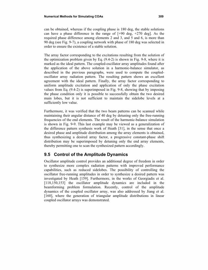
Numerical Methods for Simulating COAs 309
can be obtained, whereas if the coupling phase is 180 deg, the stable solutions can have a phase difference in the range of [+90 deg, +270 deg]. As the required phase difference among elements 2 and 3, and 5 and 6, is more than 90 deg (see Fig. 9-7), a coupling network with phase of 180 deg was selected in order to ensure the existence of a stable solution. The array factor corresponding to the excitations resulting from the solution of the optimization problem given by Eq. (9.4-2) is shown in Fig. 9-8, where it is marked as the ideal pattern. The coupled-oscillator array amplitudes found after the application of the above solution in a harmonic-balance simulator, as described in the previous paragraphs, were used to compute the coupled-oscillator array radiation pattern. The resulting pattern shows an excellent agreement with the ideal pattern. Finally, the array factor corresponding to uniform amplitude excitation and application of only the phase excitation values from Eq. (9.4-2) is superimposed in Fig. 9-8, showing that by imposing the phase condition only it is possible to successfully obtain the two desired main lobes, but it is not sufficient to maintain the sidelobe levels at a sufficiently low value. Furthermore, it was verified that the two beam patterns can be scanned while maintaining their angular distance of 40 deg by detuning only the free-running frequencies of the end elements. The result of the harmonic-balance simulation is shown in Fig. 9-9. This last example may be viewed as a generalization of the difference pattern synthesis work of Heath [31], in the sense that once a desired phase and amplitude distribution among the array elements is obtained, thus synthesizing a desired array factor, a progressive constant-phase shift distribution may be superimposed by detuning only the end array elements, thereby permitting one to scan the synthesized pattern accordingly.
9.5 Control of the Amplitude Dynamics
Oscillator amplitude control provides an additional degree of freedom in order to synthesize more complex radiation patterns with improved performance capabilities, such as reduced sidelobes. The possibility of controlling the oscillator free-running amplitudes in order to synthesize a desired pattern was investigated by Heath [159]. Furthermore, in the works of Georgiadis et al. [118,150,153] the oscillator amplitude dynamics are included in the beamforming problem formulation. Recently, control of the amplitude dynamics of the coupled oscillator array, was also addressed by Jiang et al. [160], where the generation of triangular amplitude distributions in linear coupled oscillator arrays was demonstrated.
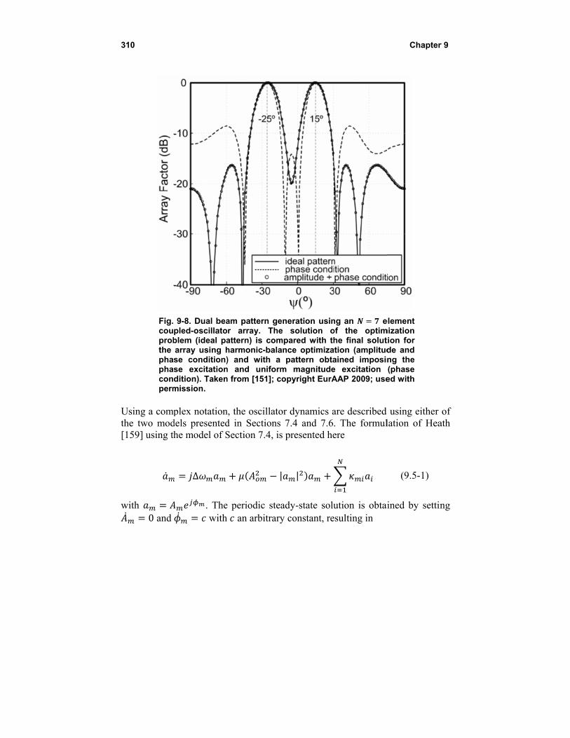
310
Fig. couprobthe phaphaconperm
Using a compthe two mod[159] using th
with 0 and
9-8. Dual beapled-oscillatoblem (ideal paarray using hse condition)se excitationdition). Takenmission.
plex notationdels presentedhe model of S
Δ
. The with
am pattern geor array. Theattern) is comharmonic-bala) and with a
n and uniformn from [151]; c
n, the oscillatod in SectionsSection 7.4, is
e periodic ste an arbitrary
eneration usine solution o
mpared with thance optimiza
pattern obtam magnitude
copyright EurA
or dynamics a 7.4 and 7.6s presented he
| |
ady-state soluy constant, re
ng an eof the optimhe final solut
ation (amplitudained imposine excitation AAP 2009; use
are described . The formulere
ution is obtaiesulting in
Chapter
element mization tion for de and ng the (phase ed with
using either lation of Hea
(9.5-1)
ined by settin
r 9
of ath
ng
Numerical Me
Fig. 9-9.oscillatoangles. permiss
with the free-runelements in ocoupling wasdesired amplabove equatparameters, examined thrEq. (9.5-1), a
9.6 Adap
In addition tadaptive recdemonstratedoscillator arr
ethods for Sim
. Dual beam por array. Osc
Taken fromion.
Δ
. Paramning frequenorder to synths considered litude and phtion into rea
and Δrough the eigas was describ
ptive Coup
to the beamfceive beamfod by Ikuma etray provides a
mulating COAs
pattern steerincillator contro
m [151]; cop
Δ
meters andncy and frehesize a desirsimplifying
ase distributial and imag
. Finally, genvalues of bed in Section
pled-Osci
forming capaormer basedt al. [154]. Tha means for c
s
ng using an ol voltages f
pyright EurAA
| |
d Δ allowe-running amred pattern. Ithe couplingon is sele
ginary parts the stabilitythe linear va
n 7.4.
llator Arra
abilities of cod on a couhe steady-statcontrolling th
elementfor different AP 2009; u
w one to indemplitude of In Ref. [159], network maected, one mand solve f
y of the soluariational equ
ay Beamfo
oupled-oscillaupled oscillate expression he array-elem
31
t coupled-scanning
used with
(9.5-2)
ependently tuthe oscillat
, near-neighbatrix . Once
may separate thfor the tuninution must b
uation given b
ormer
ator arrays, tor array wof the couple
ment amplitud
11
une tor bor e a the ng be by
an was ed-des
312 Chapter 9
and phases by adjusting the free-running oscillator frequencies and the coupling network. Similarly to the previous paragraph, a complex notation for the array dynamics pertaining to either of the two models of Sections 7.4 and 7.6 may be utilized. The formulation of Section 7.4, also shown in Eq. (9.5-1), was followed in Ref. [154]. The periodic steady-state solution is obtained by setting 0 and with an arbitrary constant, resulting in
(9.6-1)
where 1,2…
Δ
| | (9.6-2)
Finally, in matrix form one has
(9.6-3)
where is a diagonal matrix with in its main diagonal and is a vector with in its main diagonal. Matrix contains the oscillator parameters, the free-running amplitudes, and the free-running frequency offsets from . The frequency offsets can be adjusted, whereas the free-running amplitudes are fixed and assumed equal for all oscillators. Amplitude control may also be achieved using, for example, a variable attenuator or variable-gain amplifier at each oscillator output. The matrix contains the coupling-network gain and phase, and it may also be tunable. In Ref. [154], nearest neighbor coupling is assumed, which results in a bi-diagonal matrix . There are many possible combinations of and that can lead to a desired complex amplitude vector . Ikuma et al. [154] considered a reconfigurable coupling network and identical oscillators without frequency tuning, leading to a fixed matrix. As a result, the coupling matrix is used to generate the desired amplitude distributions . The proposed adaptive receiver of Ikuma et al. [154] is shown in Fig. 9-10. Assuming a receiving uniform linear-antenna array of elements, the received signal vector from all antennas is . The received signal is split into two signal paths. The signal in the first path is mixed with a reference oscillator , and after passing through a low-pass filter to remove unwanted mixing products, it provides the reference vector
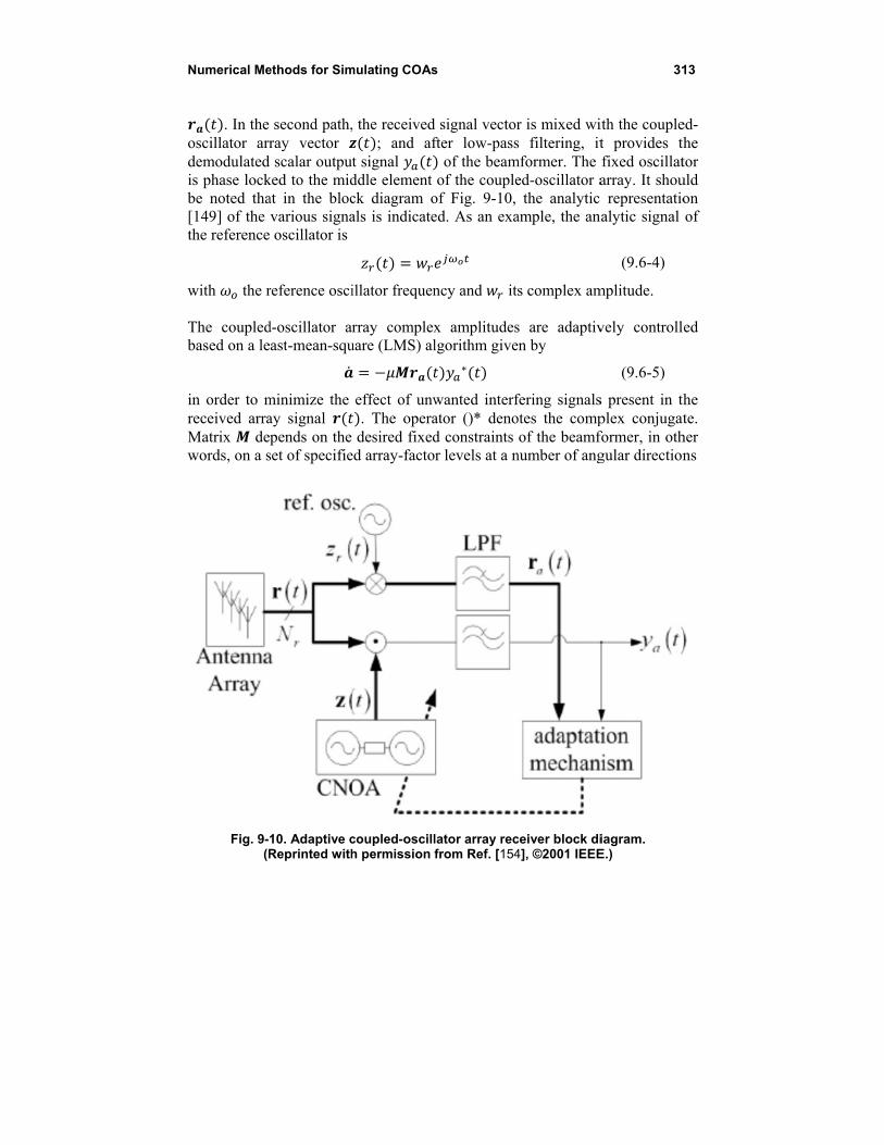
Numerical Me
. In the oscillator arrdemodulatedis phase lockbe noted tha[149] of the the reference
with the r The coupledbased on a le
in order to mreceived arraMatrix dewords, on a s
Fig. 9-(R
ethods for Sim
second path,ray vector
d scalar outpuked to the midat in the blocvarious signa oscillator is
reference osci
d-oscillator areast-mean-squ
minimize the ay signal pends on the
set of specifie
10. Adaptive cReprinted with
mulating COAs
, the received; and af
t signal ddle element ck diagram oals is indicate
illator frequen
rray complexuare (LMS) al
effect of unw. The operadesired fixed
ed array-facto
coupled-oscillh permission f
s
d signal vectorfter low-pass
of the beamof the couple
of Fig. 9-10,ed. As an exa
ncy and it
x amplitudeslgorithm give
∗
wanted interfator ()* denod constraints r levels at a n
lator array recfrom Ref. [154
r is mixed wis filtering, it
mformer. The ed-oscillator a
the analytic ample, the an
s complex am
s are adaptiven by
fering signalsotes the compof the beamf
number of ang
ceiver block di4], ©2001 IEEE
31
ith the couplet provides thfixed oscillatarray. It shou representatio
nalytic signal
(9.6-4)
mplitude.
vely controll
(9.6-5)
s present in thplex conjugatformer, in othgular direction
iagram. E.)
13
ed-the tor uld on of
ed
the te.
her ns
314 Chapter 9
including the direction of arrival of the main beam [154]. Finally, the parameter controls the convergence speed of the beamformer. The proposed
beamformer operation was verified by computer simulation.
9.7 Conclusion
In this chapter we introduced several optimization problems, demonstrating the beamforming capabilities of coupled oscillator arrays. The beamforming problem has been formulated as a convex optimization problem, which includes the array steady state as a linear constraint. The results of Chapter 7 have been used to provide an expression for the steady state of the coupled-oscillator array. Additionally, the capability of generating and scanning multiple beams has been verified. Furthermore, a non-convex optimization algorithm, which optimizes the stability of the steady state solution, has been introduced, and an adaptive beamformer based on coupled oscillator arrays has been demonstrated. The combination of optimization and signal-processing techniques (together with the rich dynamical properties of coupled-oscillator arrays) reveal the potential and numerous applications of such arrays, which have yet to be explored.

315
Chapter 10 Overall Conclusions and Possible Future
Directions
Active integrated antennas have found numerous applications as phased arrays, retro-directive arrays, and spatial power combiners. Coupled-oscillator antenna arrays represent a very exciting subset of active integrated antennas both from an application point of view, as well as from a research and analysis point of view, due to some very attractive properties, such as their ability to produce arbitrary phase shift distributions, as well as their capabilities of frequency conversion and frequency generation. In addition, they inherit the practical advantages of active integrated antennas, which are compact low-profile circuit implementations that are compatible with low-cost fabrication technologies (such as microstrip and coplanar waveguide), using single and multilayer printed circuit boards. As we have seen, however, the design of coupled-oscillator antenna arrays, is far from trivial due to their highly nonlinear nature, which results in a dynamical behavior that is difficult to simulate and predict accurately and, in effect, increases the difficulty of designing coupled-oscillator arrays demonstrating a robust performance. Nonetheless, the progress of nonlinear circuit simulation and optimization techniques and the increase in computational power of low cost personal computers has made possible the accurate analysis of coupled-oscillator arrays with as many as a few tens of elements via combining sophisticated nonlinear models for the active devices and electromagnetic analysis for the antenna, transmission lines, and interconnects, using the various methods described in Chapter 8. Efficient
316 Chapter 10
analysis of large coupled-oscillator arrays requires the use of approximate perturbation models, infinite-array approximations, and the continuum model that enable understanding of the exhibited behavior at a level permitting design of functional systems. The intuitive understanding of the array behavior and the gain in computational efficiency resulting from application of such methods makes them indispensable tools, complementary to the fully nonlinear simulators. The description and use of such methods has been the focus of Chapter 1 through Chapter 7. Interest in low-cost, high-performance radio-frequency systems with reconfigurable properties in terms of transmitted beam direction or polarization makes coupled oscillator arrays a strong candidate for many applications including radar, phased arrays, and imaging in the microwave and millimeter wave frequencies. There are still numerous challenges to be addressed and many areas where improvements in coupled-oscillator array technology are desirable. Among these we specifically note the application of new implementation technologies in the design of coupled oscillator arrays, such as substrate integrated waveguide (SIW) technology and the creation of conformal coupled-oscillator arrays using flexible substrate materials such as paper and liquid crystal polymers (LCP). Preliminary results concerning coupled-oscillator arrays using SIW technology were discussed in Chapter 6, demonstrating the possibility of low-cost single substrate array implementation. On the other hand, fully integrated coupled-oscillator arrays in the millimeter-wave frequencies have also appeared in the literature [161] paving the way for the introduction of coupled-oscillator arrays in millimeter-wave phased-array sensing and communication applications. We further note, that successful demonstrations of only small arrays have been reported in the literature to date, and large arrays employing hundreds of elements remain to be seen. In such large arrays, perimeter oscillator control of the radiated beam will be particularly beneficial. Furthermore, the demonstration of coupled-oscillator arrays using signal processing and optimization techniques in beamforming, and more importantly adaptive beamforming, is an area that should be further exploited. Finally, a number of challenging analysis problems remain to be addressed, such as quantifying the effect of phase noise on the locking range of the array and more detailed study of mode locking for pulsed operation of coupled oscillators in the microwave frequencies. Despite the progress in the theory and design of coupled-oscillator arrays during the past two decades, active antenna arrays based on coupled oscillators have not yet found widespread practical application, although there have been notable achievements in array implementations such as the ones shown in
Overall Conclusions 317
Chapter 6. It is hoped that the material presented in this book demonstrates the potential of coupled-oscillator arrays and motivates deigners to apply them in microwave and millimeter-wave array antennas. We have endeavored to provide the reader with the understanding and the tools for such application through description of the research to date and mention of a few areas for further study and technological development. The references to the archival literature will, of course, provide more detail than could be included here without rendering the presentation far too cumbersome for the casual reader. However, the literature sometimes presupposes significant familiarity with the approaches currently in vogue. Thus, in parts the present treatment is an overview of the research work while in other parts it provides a tutorial facilitating access to the literature. We hope to have struck a balance between these two styles of presentation resulting in a book of somewhat wider utility in this field than would be the case for either style alone.

318 Chapter 10
319
References
[1] K. D. Stephan, “Inter-Injection-Locked Oscillators for Power Combining and Phased Arrays,” IEEE Transactions on Microwave Theory and Techniques, vol. MTT-34, pp. 1017–1025, October 1986.
[2] K. D. Stephan and W. A. Morgan, “Analysis of Interinjection-Locked Oscillators for Integrated Phased Arrays,” IEEE Transactions on Antennas and Propagatation, vol. AP-35, no. 7, pp. 771–781, July 1987.
[3] K. D. Stephan and S.-L. Young, “Mode Stability of Radiation-Coupled Interinjection-Locked Oscillators for Integrated Phased Arrays,” IEEE Transactions on Microwave Theory and Techniques, vol. MTT-36, no. 5, pp. 921–924, May 1988.
[4] R. A. York and R. C. Compton, “Quasi-Optical Power-Combining Using Mutually Synchronized Oscillator Arrays,” IEEE Transactions on Microwave Theory and Techniques, vol. MTT-39, pp. 1000–1009, June 1991.
[5] R. A. York and R. C. Compton, “Mode-Locked Oscillator Arrays,” IEEE Microwave Guided Wave Letters, vol. 1, no. 8, pp. 215–218, August 1991.
[6] R. A. York and R. C. Compton, “Experimental Observation and Simulation of Mode-Locking in Coupled-Oscillator Arrays,” Journal of Applied Physics, vol. 71, no. 6, pp. 2959–2965, March 1992.
[7] R. A. York and R. C. Compton, “Measurement and Modeling of Radiative Coupling in Oscillator Arrays,” IEEE Transactions on Microwave Theory and Techniques, vol. MTT-41, pp. 438–444, March 1993.
320 References
[8] J. W. Mink, “Quasi-Optical Power Combining of Solid-State Millimeter-Wave Sources,” Microwave Theory and Techniques, vol. MTT-34, pp. 273–279, February 1986.
[9] B. van der Pol, “The Nonlinear Theory of Electric Oscillators,” Proceedings of the Institute of Radio Engineers, vol. 22, pp. 1051–1086, September 1934.
[10] R. Adler, “A Study of Locking Phenomena in Oscillators,” IEEE Proceedings, vol. 61, pp. 1380–1385, 1973. (Reprinted from Proceedings of the Institute of Radio Engineers, vol. 34, pp. 351–357, June 1946.)
[11] D. A. Linkens, “Analytical Solution of Large Numbers of Mutually Coupled Nearly Sinusoidal Oscillators,” IEEE Transactions on Circuits and Systems, vol. CAS-21, no. 2, pp. 294–300, March 1974.
[12] T. Endo and S. Mori, “Mode Analysis of a Ring of a Large Number of Mutually Coupled van der Pol Oscillators,” IEEE Transactions on Circuits and Systems, vol. CAS-25, no. 1, pp. 7–18, January 1978.
[13] R. H. Rand, A. H. Cohen, and P. J. Holmes, “Ch. 9 - Systems of Coupled Oscillators as Models of Central Pattern Generators,” in Neural Control of Rythmic Movements in Vertebrates. Hoboken, New Jersey: John Wiley & Sons, 1988.
[14] A. H. Cohen, P. J. Holmes, and R. H. Rand, “The Nature of the Coupling Between Segmental Oscillators of the Lamprey Spinal Generator for Locomotion: A Mathematical Model,” Journal of Mathematical Biology, vol. 13, pp. 345–369, 1982.
[15] K. Kurokawa, “Injection Locking of Microwave Solid-State Oscillators,” Proceedings of the IEEE, vol. 61, pp. 1386–1410, October 1973.
[16] H. C. Chang, E. S. Shapiro, and R. A. York, “Influence of the Oscillator Equivalent Circuit on the Stable Modes of Parallel-Coupled Oscillators,” IEEE Transactions on Microwave Theory and Techniques, vol. MTT-45, no. 8, pp. 1232–1239, 1997.
[17] S. Nogi, J. Lin, and T. Itoh, “Mode Analysis and Stabilization of a Spatial Power Combining Array with Strongly Coupled Oscillators,” IEEE Transactions on Microwave Theory and Techniques, vol. MTT-41, pp. 1827–1837, October 1993.
[18] B. K. Meadows, T. H. Heath, J. D. Neff, E. A. Brown, D. W. Fogliati, M. Gabbay, V. In, P. Hasler, S. P. Deweeth, and W. L. Ditto, “Nonlinear Antenna Technology,” Proceedings of the IEEE, vol. 90, no. 5, pp. 882–897, May 2002.
References 321
[19] V. Seetharam and L. W. Pearson, “Analysis of Strong Coupling in Coupled Oscillator Arrays,” IEEE Transactions on Antennas and Propagation, vol. AP-58, no. 4, pp. 1067–1075, April 2010.
[20] M. Armand, “On the Output Spectrum of Unlocked Driven Oscillators,” IEEE Proceedings, vol. 57, pp. 798–799, 1969.
[21] S. Sancheti and V. F. Fusco, “Active Antenna Top-Cover Frequency Pulling Effects,” IEE Proceedings on Microwave Antennas and Propagation, vol. 141, no. 5, pp. 374–376, October 1994.
[22] S. Sancheti and V. F. Fusco, “Modeling of Active Antenna Array Coupling Effects - A Load Variation Method,” IEEE Transactions on Microwave Theory and Techniques, vol. MTT-43, no. 8, pp. 1805–1808, August 1995.
[23] D. E. J. Humphrey and V. F. Fusco, “Nonlinear Two Element Active Antenna Array Stability Analysis,” Electronics Letters, vol. 32, no. 9, pp. 788–789, April 1996.
[24] D. E. J. Humphrey and V. F. Fusco, “Mode Change Analysis of a Two Element Oscillator-Type Antenna Array,” IEE Proceedings on Microwave Antennas and Propagation, vol. 144, no. 6, pp. 483–487, December 1997.
[25] D. E. J. Humphrey, V. F. Fusco, and S. Drew, “Active Antenna Array Behavior,” IEEE Transactions on on Microwave Theory and Techniques, vol. MTT-43, no. 8, pp. 1819–1824, August 1995.
[26] C. A. Lee and G. C. Dalman, “Pulse-Time Modulation of Mutually Coupled Arrays of Oscillators,” IEEE Transactions on Microwave Theory and Techniques, vol. MTT-47, no. 1, pp. 34–41, January 1999.
[27] V. Seetharam, J. Shen, and L. W. L. W. Pearson, “Effect of Coupling Phase on Mutual Injection Locking Range in Coupled Oscillator Arrays,” IEEE Transactions on Antennas and Propagation, vol. AP-57, no. 5, pp. 1391–1398, May 2009.
[28] P. Liao and R. A. York, “A New Phase Shifterless Beam-Scanning Technique Using Arrays of Coupled Oscillators,” IEEE Transactions on Microwave Theory and Techniques, vol. MTT-41, pp. 1810–1815, October 1993.
[29] T. Heath, K. Wiesenfeld, and R. A. York, “Manipulated Synchronization: Beam Steering in Phased Arrays,” International Journal of Bifurcation and Chaos, vol. 10, no. 11, pp. 2619–2627, 2000.
322 References
[30] J-H. Hwang and N-H. Myung, “A New Beam Scanning Technique by Controlling the Coupling Angle in a Couplked Oscillator Array,” IEEE Microwave and Guided Wave Letters, vol. 8, no. 5, pp. 191–193, May 1998.
[31] T. Heath, “Difference Pattern Beam Steering of Coupled, Nonlinear Oscillator Arrays,” IEEE Microwave and Wireless Components Letters, vol. 11, no. 8, pp. 343–345, August 2001.
[32] J. J. Lynch and R. A. York, “Synchronization of Oscillators Coupled Through Narrow-Band Coupling Networks,” IEEE Transactions on Microwave Theory and Techniques, vol. MTT-49, no. 2, pp. 237–249, February 2001.
[33] R. A. York, P. Liao, and J. J. Lynch, “Oscillator Array Dynamics with Broadband N-port Coupling Networks,” IEEE Transactions on Microwave Theory and Techniques, vol. MTT-42, pp. 2040–2045, November 1994.
[34] R. J. Pogorzelski, “On the Design of Coupling Networks for Coupled Oscillator Arrays,” IEEE Transactions on Antennas and Propagation, vol. AP-51, pp. 794–801, April 2003.
[35] N. Amitay, V. Galindo, and C. P. Wu, Theory and Analysis of Phased Array Antennas. New York, New York: Wiley-Interscience, 1972.
[36] D. E. J. Humphrey and V. F. Fusco, “Capacitively Coupled Oscillator Array Behaviour,” IEE Proceedings - Circuits Devices Systems, vol. 143, no. 3, pp. 167–170, June 1996.
[37] M. Abramowitz and I. Stegun, Handbook of Mathematical Functions. Washington, District of Columbia: National Bureau of Standards, 1964.
[38] R. J. Pogorzelski, P. F. Maccarini, and R. A. York, “A Continuum Model of the Dynamics of Coupled Oscillator Arrays for Phase-Shifterless Beam Scanning,” IEEE Transactions on Microwave Theory and Techniques, vol. 47, no. 4, pp. 463–470, April 1999, Correction: MTT-48, p. 1422, August 2000.
[39] R. J. Pogorzelski, P. F. Maccarini, and R. A. York, “Continuum Modeling of the Dynamics of Externally Injection-Locked Coupled Oscillator Arrayas,” IEEE Transactions on Microwave Theory and Techniques, vol. MTT-47, no. 4, pp. 471–478, April 1999, Corrections: MTT-47, p. 1147, July 1999 and MTT-48, p. 1422, August 2000.
[40] R. A. York and T. Itoh, “Injection- and Phase-locking Techniques for Beam Control,” IEEE Transactions on Microwave Theory and Techniques, vol. MTT-46, pp. 1920–1929, November 1998.
References 323
[41] J.-H. Yoon and N.-H. Myung, “Continuous Dynamics for a Linear Coupled-Oscillator Array with Peripheral Coupling-Phase Adjustments,” Microwave and Optical Technology Letters, vol. 42, no. 5, pp. 422–425, September 2004.
[42] R. J. Pogorzelski, “On the Dynamics of Two-Dimensional Array Beam Scanning via Perimeter Detuning of Coupled Oscillator Arrays,” IEEE Transactions on Antennas and Propagation, vol. AP-49, no. 2, pp. 234–242, February 2001.
[43] R. J. Pogorzelski, “Two-Dimensional Array Beam Scanning via Externally and Mutually Injection-Locked Couppled Oscillators,” IEEE Transactions on Antennas and Propagation, vol. AP-49, no. 2, pp. 243–249, February 2001.
[44] R. J. Pogorzelski, “Phased Arrays Based on Oscillators Coupled on Triangular and Hexagonal Lattices,” IEEE Transactions on Antennas and Propagation, vol. AP-52, no. 3, pp. 790–800, March 2004, Correction: AP-52, 2196, August 2004.
[45] R. J. Pogorzelski, “On the Steady State Phase Distribution in a Hexagonally Coupled Oscillator Array,” IEEE Transactions on Antennas and Propagation, vol. AP-53, pp. 4058–4064, December 2005.
[46] W. H. Press, B. P. Flannery, S. A. Teukolsky, and W. T. Vetterling, Numerical Recipies - The Art of Scientific Computing. Cambridge, United Kingdom: Cambridge University Press, 1986.
[47] R. J. Pogorzelski, “Generalization of the Linearized Discrete Model of Coupled Oscillator Arrays to Account for Coupling Delay,” Radio Science, vol. 43, no. RS4070, doi:10.1029/2007RS003727, 2008.
[48] R. J. Pogorzelski, “Continuum Modeling of Coupled Oscillator Arrays with Coupling Delay,” Radio Science, vol. 43, no. RS4S04, doi:10.1029/2007RS003741, 2008.
[49] R. J. Pogorzelski, “Beam Steering Dynamics in Coupled Oscillator Based Phased Arrays with Coupling Delay,” Radio Science, vol. 44, no. RS2019, doi:10.1029/2008RS004056, 2008.
[50] X. Wang and L. W. Pearson, “Design of Coupled-Oscillator Arrays without a Posteriori Tuning,” IEEE Transactions on Microwate Theory and Techniques, vol. MTT-53, no. 1, pp. 410–413, January 2005.
[51] J. Shen and L. W. Pearson, “The Phase Error and Beam-Pointing Error in Coupled Oscillator Beam-Steering Arrays,” IEEE Transactions on Antennas and Propagation, vol. AP-53, no. 1, pp. 386–393, January 2005.
324 References
[52] P. S. Hall and P. M. Haskins, “Microstrip Active Patch Array with Beam Scanning,” Electronics Letters, vol. 28, no. 22, pp. 2056–2057, October 1992.
[53] R. A. York, “Nonlinear Analysis of Phase Relationships in Quasi-Optical Oscillator Arrays,” IEEE Transactions on Microwave Theory and Techniques, vol. MTT-41, no. 10, pp. 1799–1809, October 1993.
[54] P. Liao and R. A. York, “A Six-Element Beam Scanning Array,” IEEE Microwave and Guided Wave Letters, vol. 4, no. 1, pp. 20–22, January 1994.
[55] R. Ispir, S. Nogi, M. Sanagi, and K. Fukui, “Transmission-Line Coupling of Active Microstrip Antennas for One- and Two-Dimensional Phased Arrays,” IEICE Transactions on Electronics, vol. E80-C, no. 9, pp. 1211-1220, September 1997.
[56] T. Kagawa, S. Nogi, and M. Sanagi, “Spatial Power Combining and Phased-Array Behavior of Circularly Polarized Active Patch Antennas,” IEICE Transactions on Electronics, vol. E82-C, no. 7, pp. 1182–1187, July 1999.
[57] R. Ispir, S. Nogi, and M. Sanagi, “Wide Angle Phase-Shifterless Beam Scanning in Unilaterally Coupled Active Antenna Arrays,” IEICE Transactions on Electronics, vol. E82-C, no. 7, pp. 1188–1194, July 1999.
[58] J. J. Lynch, H.-C. Chang, and R. A. York, “Coupled-Oscillator Arrays and Scanning Techniques,” in Active and Quasi-Optical Arrays for Solid-State Power Combining. Hoboken, New Jersey: John Wiley & Sons, 1997, pp. 135–183.
[59] H.-C. Chang, X. Cao, M. J. Vaughn, U. K. Mishra, and R. A. York, “Phase Noise in Externally Injection Locked Oscillator Arrays,” IEEE Transactions on on Microwave Theory and Techniques, vol. MTT-45, no. 11, pp. 2035–2042, November 1997.
[60] R. J. Pogorzelski, R. P. Scaramastra, J. Huang, R. J. Beckon, S. M. Petree, and C. Chavez, “A Seven Element S-Band Coupled Oscillator Controlled Agile Beam Phased Array,” IEEE Transactions on Microwave Theory and Techniques, vol. MTT-48, no. 8, pp. 1375–1384, August 2000.
[61] R. J. Pogorzelski, “A Two-Dimensional Coupled Oscillator Array,” IEEE Microwave and Guided Wave Letters, vol. 10, pp. 478–480, November 2000.
References 325
[62] R. J. Pogorzelski, “Coupled Oscillator Based Agile Beam Transmitters and Receivers: A Review of Work at JPL,” Proceedings of the 2006 IEEE Aerospace Conference (Big Sky, Montana, March 14–16, 2006), 0-7803-9546-8/06, 2006.
[63] R. J. Pogorzelski, “Experimental Confirmation of the Dynamics of Coupled Oscillator Arrays,” IEEE Tranactions on Microwave Theory and Techniques, vol. MTT-50, no. 1, pp. 143–149, January 2002.
[64] F. Shigeki, “Waveguide Line (in Japanese),” Japan Patent 06-053711, February 25, 1994.
[65] F. Giuppi, A. Georgiadis, M. Bozzi, A. Collado, and L. Perregrini, “Active Antenna Oscillator Systems in Substrate Integrated Waveguide (SIW) Technology,” presented at Proceedings of the Fourth European Conference on Antennas and Propagation (EuCAP), Barcelona, Spain, 2010.
[66] M. Bozzi, L. Perregrini, K. Wu, and P. Arcioni, “Current and Future Research Trends in Susbtrate Integrated Waveguide Technology,” Radioengineering, vol. 18, no. 2, pp. 201–209, June 2009.
[67] N. Karmakar, “Investigations into a Cavity-Backed Circular Patch Antenna,” IEEE Transactions on Antennas and Propagation, vol. 50, no. 12, pp. 1706–1715, December 2002.
[68] F. Giuppi, A. Georgiadis, A. Collado, M. Bozzi, and L. Perregrini, “Tunable SIW Cavity Backed Active Antenna Oscillator,” The Institution of Engineering and Technology (IET) Electronics Letters, vol. 46, no. 5, pp. 1053–1055, July 22, 2010.
[69] R. J. Pogorzelski, “A Frequency Tripled Two-Dimensional Coupled Oscillator Array,” IEEE Transactions on Antennas and Propagation, vol. AP-52, no. 3, pp. 907–910, March 2004.
[70] R. J. Pogorzelski, “A Five by Five Element Two-Dimensional Coupled Oscillator Array,” IEEE Transactions on Antennas and Propagation, vol. AP-53, no. 4, pp. 1337–1345, April 2005.
[71] T. Heath, R. R. Kerr, and G. D. Hopkins, “Two Dimensional Nonlinear Oscillator Array Antenna,” Proceedings IEEE Aerospace Conference, 2005.
[72] S.-C. Yen and T.-H. Chu, “A Beam-Scanning and Polarization-Agile Antenna Array Using Mutually Coupled Oscillating Doublers,” IEEE Transactions on Antennas and Propagation, vol. 53, no. 12, pp. 4051–4057, December 2005.
326 References
[73] X. Cao and R. A. York, “Coupled Oscillator Scanning Techniques for Receiver Applications,” IEEE Antennas And Propagation Symposium Digest, pp. 1311–1314, 1995.
[74] R. J. Pogorzelski and F. Chiha, “A Demonstration of the Coupled Oscillator Based Agile Beam Receiver Concept,” IEEE Transactions on Antennas and Propagation, vol. AP-53, no. 11, pp. 3584–3588, DOI: 10.1109/TAP.2005.858835, November 2005.
[75] M. A. Kott, Phased Array with Wide Null, U.S. Patent 5,343,211, August 30 1994.
[76] R. J. Pogorzelski, “On a Simple Method of Obtaining Sidelobe Reduction over a Wide Angular Range in One and Two Dimensiions,” IEEE Transactions on Antennas and Propagation, vol. AP-49, pp. 475–482, March 2001.
[77] G. S. Shiroma, R. Y. Miyamoto, and W. A. Shiroma, “A 16-Element Two-Dimensional Active Self-Steering Array Using Self-Oscillating Mixers,” IEEE Transactions on Microwave theory and Techniques, vol. 51, no. 12, pp. 2476–2482, December 2003.
[78] M. Sanagi, J. Fujiwara, K. Fujimori, and S. Nogi, “Beam Control in Unilaterally Coupled Active Antennas with Self-Oscillating Harmonic Mixers,” IEICE Transactions on Electronics, vol. E88-C, no. 7, pp. 1375–1381, July 2005.
[79] S. V. Hoeye, C. Vazquez, M. Fernandez, F. L. Herran, and F. Las-Heras, “Receiving Phased Antenna Array Based on Injection-Locked Harmonic Self-Oscillating Mixers,” IEEE Transactions on Antennas and Propagation, vol. 57, pp. 645–651, Mar. 2009.
[80] S. V. Hoeye, L. F. Herran, M. Fernandez, and F.L. Heras, “Design and Analysis of a Microwave Large-Range Variable Phase-Shifter Based on an Injection-Locked Harmonic Self-Oscillating Mixer,” IEEE Microwave and Wireless Components Letters, vol. 16, no. 6, pp. 342–344, June 2006.
[81] H.-C. Chang, A. Borgioli, P. Yeh, and R. A. York, “Analysis of Oscillators with External Feedback Loop for Improved Locking Range and Noise Reduction,” IEEE Transactions on Microwave Theory and Techniques, vol. MTT-47, no. 8, pp. 1535–1543, August 1999.
[82] M. Zheng, P. Gardener, P. S. Hall, Y. Hao, Q. Chen, and V. F. Fusco, “Cavity Control of Active Integrated Antenna Oscillators,” IEE Proceedings on Microwave Antennas and Propagation, vol. 148, no. 1, pp. 15–20, February 2001.
References 327
[83] M. Colwell and L. W. Pearson, “Enhancement of Locking Range Through Reactive Loading on the Feedback Path,” IEEE Microwave and Wireless Components Letters, vol. 13, no. 9, pp. 417–419, September 2003.
[84] H.-C., Chang, X. Cao, U. K. Mishra, and R. A. York, “Phase Noise in Coupled Oscillators: Theory and Experiment,” IEEE Transactions on Microwave Theory and Techniques, vol. MTT-45, no. 5, pp. 604–615, May 1997.
[85] M. Nick, A. Banai, and F. Farzaneh, “Phase Noise Measurement Using Two Inter-Injection Locked Microwave Oscillators,” IEEE Transactions on Microwave Theory and Techniques, vol. MTT-54, no. 7, pp. 2993–3000, July 2006.
[86] L. Dussopt and J.-M. Laheurte, “Coupled Oscillator Array Generating Circular Polarization,” IEEE Microwave and Guided Wave Letters, vol. 94, pp. 160–162, April 1999.
[87] L. Dussopt and J.-M. Laheurte, “Phase Noise Improvement in a Loop Configuration of Oscillating Antennas,” IEEE Microwave and Guided Wave Letters, vol. 10, no. 3, pp. 111–113, March 2000.
[88] S. Yang, V. F. Fusco, and D. E. J. Humphrey, “Ring-Coupled-Oscillator Sequentially Rotated Active Antenna,” IEEE Transactions on Microwave Theory and Techniques, vol. MTT-49, no. 8, pp. 1492–1497, August 2001.
[89] J. J. Lynch and R. A. York, “Stability of Mode Locked States of Coupled Oscillator Arrays,” IEEE Transactions on Circuits and Systems -I: Fundamental Theory and Applications, vol. 42, no. 8, pp. 413–418, August 1995.
[90] J. J. Lynch and R. A. York, “An Analysis of Mode-Locked Arrays of Automatic Level Control Oscillators,” IEEE Transactions on Circuits and Systems I: Fundamental Theory and Applications, vol. 41, no. 12, pp. 859–865, December 1994.
[91] R. R. Ram, R. Sporer, H.-R. Blank, and R. A. York, “Chaotic Dynamics in Coupled Microwave Oscillators,” IEEE Transactions on Microwave Theory and Techniques, vol. MTT-48, no. 11, pp. 1909–1916, November 2000.
[92] R. D. Martinez and R. C. Compton, “Electronic Beamsteering of Active Arrays With Phase-Locked Loops,” IEEE Microwave and Guided Wave Letters, vol. 4, no. 6, pp. 166–168, June 1994.
328 References
[93] J. J. Lynch and R. A. York, “A Mode Locked Array of Coupled Phase Locked Loops,” IEEE Microwave and Guided Wave Letters, vol. 5, no. 7, pp. 213–215, July 1995.
[94] D. W. Jordan and P. Smith, Nonlinear Ordinary Differential Equations: An Introduction to Dynamical Systems, 3rd Ed. Oxford, United Kingdom: Oxford University Press, 1999.
[95] R. A. York, P. Liao, and J. J. Lynch, “Oscillator Array Dynamics with Broadband N-Port Coupling Networks,” IEEE Transactions on Microwave Theory and Techniques, pp. 2040–2045, November 1994.
[96] T. Heath, “Simultaneous Beam Steering and Formation with Coupled, Nonlinear Oscillator Arrays,” IEEE Transactions on Antennas and Propagation, vol. 53, no. 6, pp. 2031–2035, June 2005.
[97] H.-C. Chang, X. Cao, U. K. Mishra, and R.A. York, “Phase Noise in Coupled Oscillators: Theory and Experiment,” IEEE Transactions on Microwave Theory and Techniques, pp. 604–615, May 1997.
[98] R. J. Pogorzelski, “Experimental Confirmation of the Dynamics of Coupled-Oscillator Arrays and Implications for Angle-Based Modulation,” IEEE Transactions on Microwave Theory and Techniques, vol. 50, no. 1, pp. 143–149, January 2002.
[99] C. Kykkotis, P.S. Hall, and H. Ghafouri-Shiraz, “Performance of Active Antenna Oscillator Arrays under Modulation for Communication Systems,” IEE Proceedings on Microwaves, Antennas and Propagation, vol. 145, no. 4, pp. 313–320, 1998.
[100] J. Guckenheimer and P. Holmes, Nonlinear Oscillations, Dynamical Systems, and Bifurcations of Vector Fields (Applied Mathematical Sciences Vol. 42). New York, New York: Springer-Verlag, 1983.
[101] T. S. Parker and L. O. Chua, Practical Numerical Algorithms for Chaotic Systems. New York, New York: Springer-Verlag, 1989.
[102] Y. A. Kuznetsov, Elements of Applied Bifurcation Theory, 2nd ed. New York, New York: Verlag, Springer, 1998.
[103] J. A. Sanders and F. Velhurst, Averaging Methods in Nonlinear Dynamical Systems. New York, New York: Springer Verlag, 1985.
[104] N. M. Krylov and N. N. Bogoliubov, New Methods of Nonlinear Mechanics in their Application to the Investigation of the Operation of Electronic Generators. Moscow, Russia: United Scientific and Technical Press, 1934.

References 329
[105] K. Kurokawa, “Noise In Synchronized Oscillators,” IEEE Transactions on Microwave Theory and Techniques, vol. 16, no. 4, pp. 234–240, April 1968.
[106] A. C. Scott, “Distributed Multimode Oscillators of One and Two Spatial Dimensions,” IEEE Transactions on Circuit Theory, vol. 17, no. 1, pp. 55–60, February 1970.
[107] H. M. Aumann, “Standing Waves on a Multimode Ladder Oscillator,” IEEE Transactions on Circuits and Systems, vol. 21, no. 3, pp. 461–462, May 1974.
[108] T. Endo and S. Mori, “Mode Analysis in a Multimode Ladder Oscillator,” IEEE Transactions on Circuits and Systems, vol. 23, no. 2, pp. 100–113, February 1976.
[109] T. Endo and S. Mori, “Mode Analysis of a Two-Dimensional Low-Pass Multimode Oscillator,” IEEE Transactions on Circuits and Systems, vol. 23, no. 9, pp. 517–530, September 1976.
[110] R. A. York and R. C. Compton, “Quasi-Optical Power-Combining Using Mutually Synchronized Oscillator Arrays,” IEEE Transactions on Microwave Theory and Techniques, vol. MTT-39, pp. 1000–1009, June 1991.
[111] R. A. York, “Nonlinear Analysis of Phase Relationships in Quasi-Optical Coupled Oscillator Arrays,” IEEE Transactions on Microwave Theory and Techniques, vol. 43, no. 10, pp. 1799–1809, October 1993.
[112] T. Heath, “Beam Steering of Nonlinear Oscillator Arrays Through Manipulation of Coupling Phases,” IEEE Transactions on Antennas and Propagation, vol. 52, no. 7, pp. 1833–1842, July 2004.
[113] Y. Kuramoto, Chemical Oscillations, Waves and Turbulence. Berlin, Germany: Springer Verlag, 1984.
[114] D.E.J. Humphrey, V.F. Fusco, and S. Drew, “Active Antenna Array Behavior,” IEEE Transactions on Microwave Theory and Techniques, vol. 43, no. 8, pp. 1819–1925, August 1995.
[115] K. Y. Chen, P. D. Biernacki, A. Lahrichi, and A. Mickelson, “Analysis of an Experimental Technique for Determining Van der Pol Parameters of a Transistor Oscillator,” IEEE Transactions on Microwave Theory and Techniques, vol. 46, no. 7, pp. 914–922, July 1998.
330 References
[116] A. Georgiadis, A. Collado, and A. Suarez, “New Techniques for the Analysis and Design of Coupled Oscillator Systems,” IEEE Transactions on Microwave Theory and Techniques, vol. 54, no. 11, pp. 3864–3877, November 2006.
[117] J.J. Lynch and R.A. York, “Synchronization of Oscillators Coupled Through Narrow-band Networks,” IEEE Transactions on Microwave Theory and Techniques, pp. 237–249, February 2001.
[118] A. Georgiadis, A. Collado, and A. Suarez, “Pattern Nulling in Coupled Oscillator Antenna Arrays,” IEEE Transactions on Antennas and Propagation, vol. 55, no. 5, pp. 1267–1274, May 2007.
[119] A. S. Lewis and M. L. Overton, “Eigenvalue Optimization,” Acta Numerica, vol. 5, pp. 149–190, 1996.
[120] A. Georgiadis and A. Collado, “Injection Locked Coupled Oscillator Arrays,” IEEE Microwave and Wireless Components Letters, pp. 900–902, Dec. 2007.
[121] C. Kykkotis, P. S. Hall, H. Ghafouri-Shiraz, and D. Wake, “Modulation Effects in Active Integrated Locked Antenna Oscillator Arrays,” in IEE Tenth International Conference on Antennas and Propagation, (Conf. Pub. No. 436), 1997, pp. 510–513.
[122] D. T. Auckland, J. Lilly, and R. A. York, “Analysis of Beam Scanning and Data Rate Transmission Performance of a Coupled Oscillator Phased Array,” in IEE Tenth International Conference on Antennas and Propagation (Conf. Publ.No. 436), 1997, pp. 245–249.
[123] H.-C. Chang, X. Cao, M. J. Vaughan, U.K. Mishra, and R. A. York, “Phase Noise in Externally Injection-Locked Oscillator Arrays,” IEEE Transactions on Microwave Theory and Techniques, vol. 45, no. 11, pp. 2035–2042, November 1997.
[124] A. Collado and A. Georgiadis, “Performance of Coupled Oscillator Arrays with Angle-Modulated Injection Signals,” IEEE Transactions on Circuits and Systems I, vol. 57, no. 9, pp. 2343–2352, 2010.
[125] R. J. Pogorzelski, S. Stride, J. Venkatesan, and M. Zawadzki, “A Seven Element X-Band Agile Beam Receiver,” in IEEE International Symposium on Antennas and Propagation (June 9–15, 2007), Honolulu, Hawaii (June 9–15, 2007), 2007, pp. 1925–1928.
[126] R. D. Martinez and R. C. Compton, “Electronic Beamsteering of Active Arrays with Phase-Locked Loops,” IEEE Microwave and Guided Wave Letters, vol. 4, no. 6, pp. 166–169, June 1994.
References 331
[127] J. F. Buckwalter, T. H. Heath, and R. A. York, “Synchronization Design of a Coupled Phase-Locked Loop,” IEEE Transactions on Microwave Theory and Techniques, vol. 51, no. 3, pp. 952–960, March 2003.
[128] H.-C. Chang, “Analysis of Coupled Phase-Locked Loops with Independent Oscillators for Beam Control active phased arrays,” IEEE Transactions on Microwave Theory and Techniques, vol. 52, no. 3, pp. 1059–1066, March 2004.
[129] K. Kurokawa, “Some Basic Characteristics of Negative Resistance Oscillator Circuits,” Bell System Technical Journal, vol. 61, pp. 1937–1955, July–August 1969.
[130] X. Lai and J. Roychowdhury, “Capturing Oscillator Injection Locking via Nonlinear Phase-Domain Macromodels,” IEEE Transactions on Microwave Theory and Techniques, vol. 52, no. 9, pp. 2251–2261, September 2004.
[131] F. Giannini and G. Leuzzi, Nonlinear Microwave Circuit Design. New York, New York: John Wiley and Sons, 2004.
[132] K. S. Kundert, J. K. White, and A. Sangiovanni-Vincentelli, Steady-State Methods For Simulating Analog and Microwave Circuits. Norwell, Massachussetts: Kluwer Academic Publishers, 1990.
[133] S. Boyd and L. Vandenberghe, Convex Optimization. Cambridge, UK: Cambridge University Press, 2004.
[134] V. Rizzoli and A. Neri, “State of the Art and Present Trends in Nonlinear Microwave CAD Techniques,” IEEE Transactions on Microwave Theory and Techniques, vol. 36, no. 2, pp. 343–365, February 1988.
[135] D. Sharrit, “Method for Simulating a Circuit,” U.S. Patent 5588142, December 24, 1996.
[136] E. Ngoya and R. Larcheveque, “Envelope Transient Analysis: A New Method for the Transient and Steady State Analysis of Microwave Communication Circuits and Systemms,” in IEEE MTT-S International Microwave Symposium, San Francisco, California, 1996, pp. 1365–1368.
[137] L. O. Chua, “A Switching Parameters Algorithm for Finding Multiple Solutions of Non-Linear Resistive Circuits,” International Journal of Circuit Theory and Applications, vol. 4, pp. 215–239, July 1976.
[138] Ch.-R. Chang, M. B. Steer, S. Martin, and E. Reese Jr., “Computer-Aided Analysis of Free-Running Microwave Oscillators,” IEEE Transactions on Microwave Theory and Techniques, vol. 39, no. 10, pp. 1735–1745, October 1991.
332 References
[139] R. Quere, E. Ngoya, M. Camiade, A. Suarez, M. Hessane, and J. Obregon, “Large Signal Design of Broadband Monolithic Microwave Frequency Dividers and Phase-Locked Oscillators,” IEEE Transactions on Microwave Theory and Techniques, vol. 41, no. 11, pp. 1928–1938, November 1993.
[140] A. Suarez and S. Sancho, “Application of the Envelope-Transient Method to the Analysis and Design of Autonomous Circuits,” International Journal of RF and Microwave Computer-Aided Engineering, vol. 15, no. 6, pp. 523–535, 2005.
[141] J. M. T. Thompson and H. B. Stewart, Nonlinear Dynamics and Chaos, 2nd ed. Chichester, West Sussex, United Kingdom: John Wiley and Sons, 2002.
[142] P. Liao and R. A. York, “A New Phase Shifterless Beam-Scanning Technique Using Arrays of Coupled Oscillators,” IEEE Transactions on Microwave Theory and Techniques, vol. MTT-41, pp. 1810–1815, October 1993.
[143] A. Georgiadis, “A Model for Stability, Noise and Angle Modulation Analysis of Injection-Locked Oscillators,” IEEE Transactions on Microwave Theory and Techniques, vol. 56, no. 4, pp. 826–834, April 2008.
[144] R. J. Pogorzelski, P. F. Maccarini, and R. A. York, “Continuum Modeling of the Dynamics of Externally Injection-Locked Coupled Oscillator Arrays,” IEEE Transactions on Microwave Theory and Techniques, vol. 47, no. 4, pp. 471–478, April 1999.
[145] A. Alexanian, H.-C. Chang, and R. A. York, “Enhanced Scanning Range of Coupled Oscillator Arrays Utilizing Frequency Multipliers,” in IEEE International Symposium on Antennas and Propagation (AP-S) Symposium Digest, Newport Beach, California, 1995, pp. 1308–13010.
[146] M. Sanagi, K. Yano, K. Fujimori, and S. Nogi, “Active Phased Array Antenna Radiating Second Harmonic Output Wave,” Electronics and Communications in Japan, Part 2, vol. 89, no. 4, pp. 39–50, DOI: 10.1002/ecjb.20168, April 2006.
[147] A. Georgiadis, “Design of Coupled Oscillator Arrays for Second Harmonic Radiation,” in IEEE MTT-S International Microwave Symposium Digest, Honolulu, Hawaii, June 2007, pp. 1727–1730.
References 333
[148] L. F. Herran, S. V. Hoeye, and F. Las Heras, “Nonlinear Optimization Tools for the Design of Microwave High-Conversion Gain Harmonic Self-Oscillating Mixers,” IEEE Microwave and Wireless Components Letters, vol. 16, no. 1, pp. 16–18, January 2006.
[149] J. G. Proakis and M. Salehi, Digital Communications, 5th ed. New York, New York: The McGraw-Hill Companies, 2008.
[150] A. Georgiadis and K. Slavakis, “A Convex Optimization Method for Constrained Beam-Steering in Planar (2-D) Coupled Oscillator Antenna Arrays,” IEEE Transactions on Antennas and Propagation, vol. 55, no. 10, pp. 2925–2928, October 2007.
[151] A. Georgiadis and A. Collado, “Multibeam Pattern Generation Using Coupled Oscillator Arrays,” in Proceedings of 3rd European Conference on Antennas and Propagation (EuCAP, March 23–27, 2009), Berlin, Germany, 2009.
[152] T. Heath, “Difference Pattern Beam Steering of Coupled, Nonlinear Oscillator Arrays,” IEEE Microwave and Wireless Components Letters, vol. 11, no. 8, pp. 343–345, November 2001.
[153] A. Georgiadis and K. Slavakis, “Stability Optimization of the Coupled Oscillator Array Steady State Solution,” IEEE Transactions on Antennas and Propagation, vol. 58, no. 2, pp. 608–612, February 2010.
[154] T. Ikuma, A. A. Beeks, J. R. Zeidler, and B. K. Meadows, “Adaptive Interference Mitigation with a Coupled Nonlinear Oscillator Array Beamformer,” in IEEE Aerospace Conference, Big Sky, Montana, 2006, pp. 1–13.
[155] I. Nesterov, A. Nemirovskii, and Y. Nesterov, Interior Point Polynomial Methods in Convex Programming;vol. 13, Studies in Applied Mathematics. Philadelphia, Pennsylvania: Society for Industrial and Applied Mathematics, 1994.
[156] S. Boyd, L. El Ghaoui, E. Feron, and V. Balakrishnan, Linear Matrix Inequalities in System and Control Theory. Philadelphia, USA: SIAM Studies in Applied Mathematics, vol. 15, 1994.
[157] H. Steyskal, “Simple Method for Pattern Nulling by Phase Perturbation,” IEEE Transactions on Antennas and Propagation, vol. AP-31, no. 1, pp. 163–166, January 1983.
[158] H. Lebret and S. Boyd, “Antenna Array Pattern Synthesis via Convex Optimization,” IEEE Transactions on Signal Processing, vol. 45, no. 3, pp. 526–532, March 1997.
334 References
[159] T. Heath, “Beam Shaping of Coupled Nonlinear-Oscillator Arrays,” in Proceedings of the SPIE, vol. 4374, 2001, pp. 114–122.
[160] H. Jiang and R. Penno, “Effects of Amplitude Dynamics on Beam Steering and Shaping in Coupled Oscillator Array,” IEEE Antennas and Wireless Propagation Letters, vol. 9, pp. 474–477, 2010.
[161] J. F. Buckwalter, A. Babakhani, A. Komijani, and A. Hajimiri, “An Integrated Subharmonic Coupled-Oscillator Scheme for a 60-GHz Phased Array Transmitter,” IEEE Transactions on Microwave Theory and Techniques, vol. 54, Part 2, no. 12, pp. 4271–4280, December 2006.
335
Acronyms and Abbreviations
AACS attitude and articulation control subsystem
ABET, Inc. Accreditation Board for Engineering and Technology
ACORDE Advanced Communications Research and Development, S.A. (Santander, Spain)
AG auxiliary generator
AM amplitude modulation
BMDO U. S. Ballistic Missile Defense Organization
CMOS complementary metal oxide semiconductor
COA coupled-oscillator array
CPG central pattern generator
CPM constant-phase modulation
CTTC Centre Tecnologic de Telecomunicacions de Catalunya (Barcelona, Spain)
dBc decibels relative to the carrier
dBm decibels referenced to milliwatts

336 Acronyms and Abbreviations
dc, DC direct current
DC bias bias voltage associated with a direct-current system
d.e. differential equation
deg degree
E-plane plane containing the electric field intensity vector
Eq. Equation
EuCAP European Conference on Antennas and Propagation
FET field effect transistor
FFT fast Fourier transform
GCD Global Communications Devices (North Andover, Massachusetts)
GHz gigahertz
GMSK Gaussian minimum-shift keying
GSM Global System for Mobile Communications
GTRI Georgia Tech Research Institute
H-plane plane containing the magnetic field intensity vector
HSOM harmonic self-oscillating mixer
IEE Institution of Electrical Engineers
IEEE Institute of Electrical and Electronics Engineers
IET Institution of Engineering and Technology
IRE Institute of Radio Engineers
IF intermediate frequency
ILR inverse locking range
Acronyms and Abbreviations 337
JPL Jet Propulsion Laboratory
L-band frequency range between 390 and 1550 MHz
LCP liquid-crystal polymers
LMDS local multipoint distribution service
LMS least mean square
MESFET metal semiconductor field-effect transistor
MHz megahertz
MMIC monolithic microwave integrated circuit
mr milliradian
Ms–1 mega inverse seconds
NARRA Novel Architectures for Reconfigurable Reflectarrays and Phased Array Antennas
NASA National Aeronautics and Space Administration
nH nanohenry
ns nanosecond
pF picofarad
pHEMT pseudomorphic high electron mobility transistor
PLL phase-locked loop
PM phase modulation
R.A.C. Radio Antenna Communications (Milan, Italy)
Ref. reference
RF radio frequency
RFCSET RF/Microwave Communication Subsystems for Emerging Wireless Technologies
RFID radio-frequency identification

338 Acronyms and Abbreviations
RLC resistance, inductance, capacitance
RoM reduced order model
S-band RF frequencies 1550–5200 MHz
SIW substrate integrated waveguide
SOM self-oscillating mixer
SWAP (Marie Curie Industry-Academia Pathways and Partnerships project) Symbiotic Wireless Autonomous Powered system
USNC/URSI U.S. National Committee (USNC) of the Union Radio Scientifique Internationale
UWB ultra-wideband
V volt
VCO voltage- controlled oscillator
VHF very high frequency
VNA vector network analyzer
VSA vector signal analyzer