course evaluations 4 random individuals will win an ati radeon tm hd2900xt
TRANSCRIPT
Course EvaluationsCourse Evaluations
http://www.siggraph.org/courses_evaluation
4 Random Individuals will win an ATI Radeontm HD2900XT
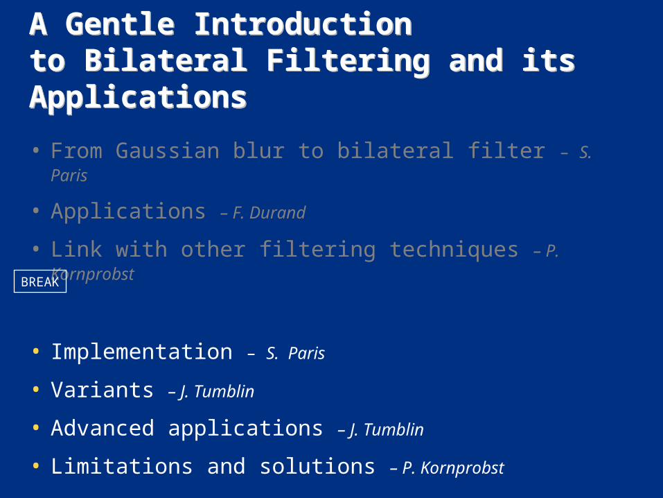
A Gentle Introduction to Bilateral Filtering and its ApplicationsA Gentle Introduction to Bilateral Filtering and its Applications
• From Gaussian blur to bilateral filter – S. Paris
• Applications – F. Durand
• Link with other filtering techniques – P. Kornprobst
• Implementation – S. Paris
• Variants – J. Tumblin
• Advanced applications – J. Tumblin
• Limitations and solutions – P. Kornprobst
BREAK
A Gentle Introductionto Bilateral Filteringand its Applications
A Gentle Introductionto Bilateral Filteringand its Applications
Recap
Sylvain Paris – MIT CSAIL
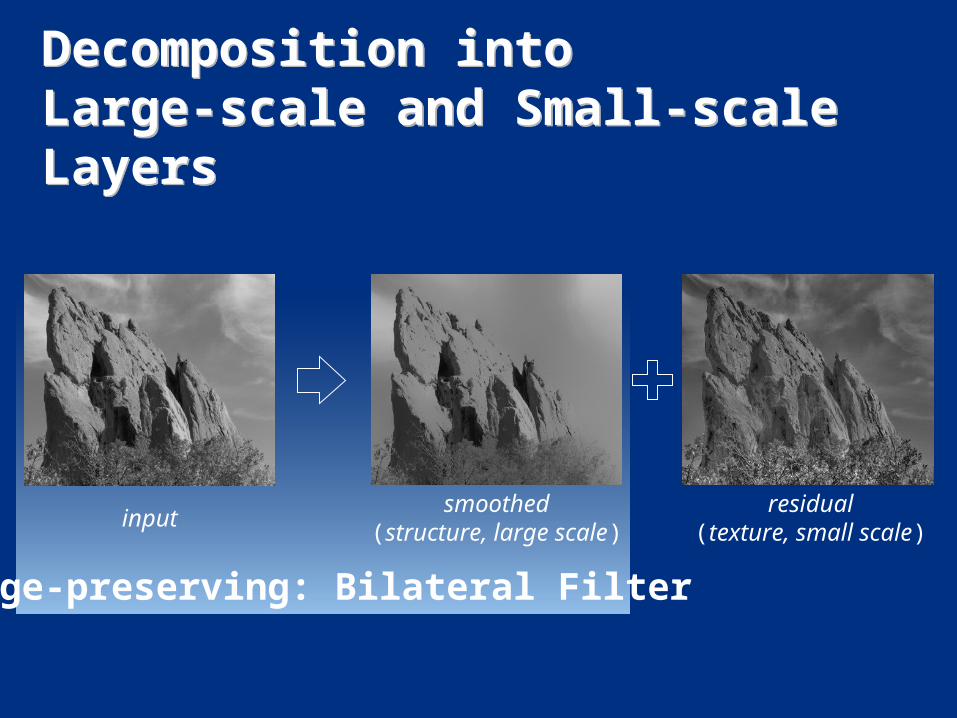
inputsmoothed
(structure, large scale)residual
(texture, small scale)
edge-preserving: Bilateral Filter
Decomposition into Large-scale and Small-scale LayersDecomposition into Large-scale and Small-scale Layers
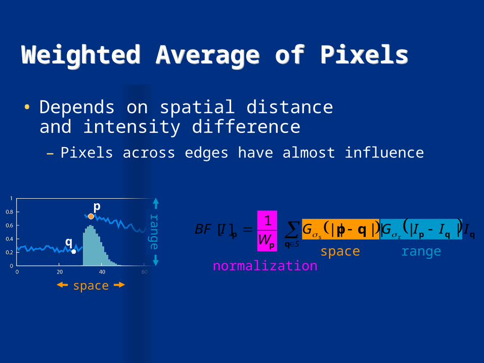
Weighted Average of PixelsWeighted Average of Pixels
space rangenormalization
S
IIIGGW
IBFq
qqpp
p qp ||||||1
][rs
space
range
p
q
• Depends on spatial distanceand intensity difference– Pixels across edges have almost influence
A Gentle Introductionto Bilateral Filteringand its Applications
A Gentle Introductionto Bilateral Filteringand its Applications
Efficient Implementationsof the Bilateral Filter
Sylvain Paris – MIT CSAIL
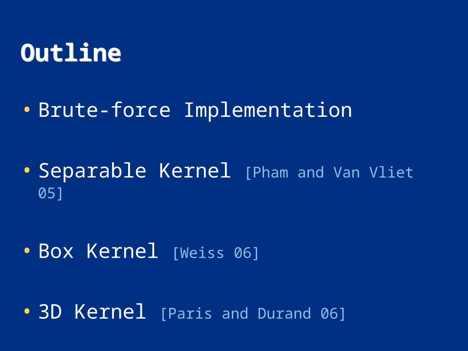
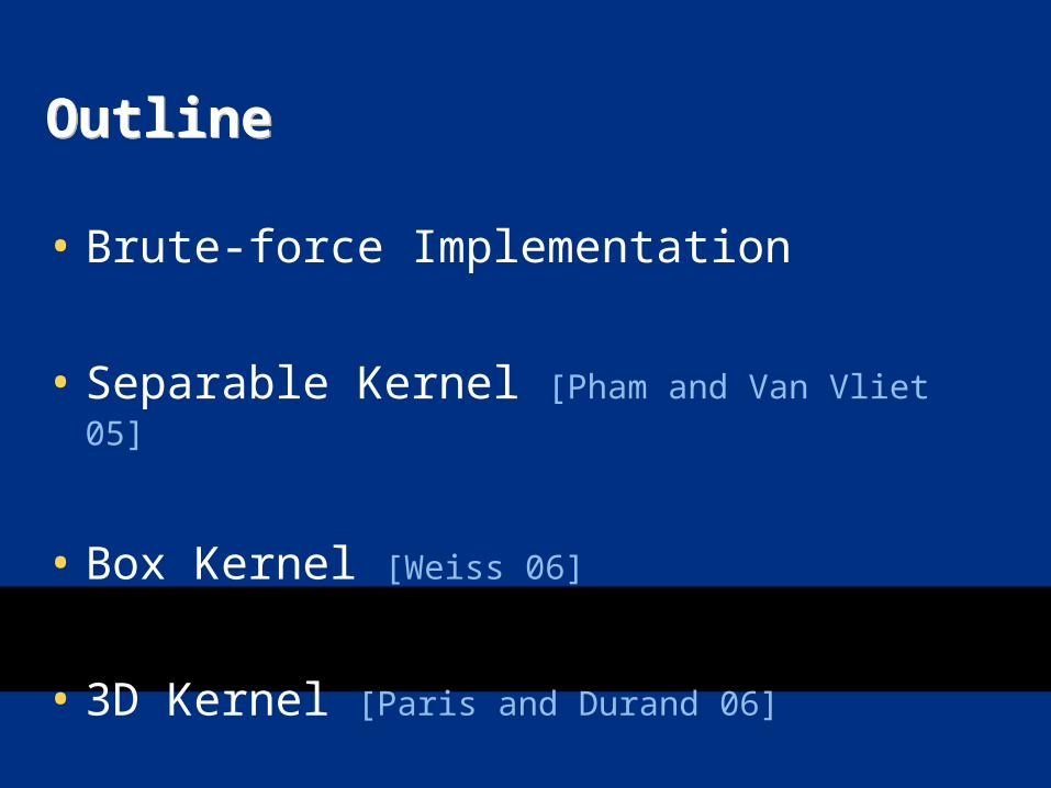
OutlineOutline
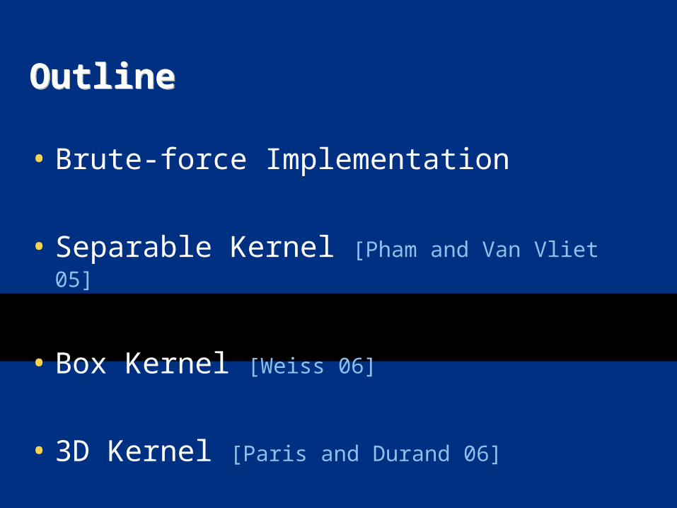
• Brute-force Implementation
• Separable Kernel [Pham and Van Vliet 05]
• Box Kernel [Weiss 06]
• 3D Kernel [Paris and Durand 06]
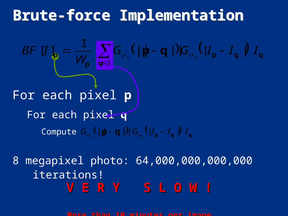
Brute-force ImplementationBrute-force Implementation
For each pixel p
For each pixel q
Compute
8 megapixel photo: 64,000,000,000,000 iterations!
V E R Y S L O W !V E R Y S L O W !
More than 10 minutes per imageMore than 10 minutes per image
S
IIIGGW
IBFq
qqpp
p qp ||||||1
][rs
qqpqp IIIGG ||||||rs
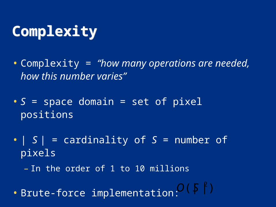
ComplexityComplexity
• Complexity = “how many operations are needed, how this number varies”
• S = space domain = set of pixel positions
• | S | = cardinality of S = number of pixels
– In the order of 1 to 10 millions
• Brute-force implementation: )|(| 2SΟ
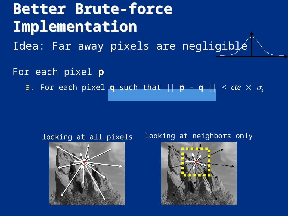
Better Brute-force ImplementationBetter Brute-force Implementation
Idea: Far away pixels are negligible
For each pixel p
a. For each pixel q such that || p – q || < cte s
looking at all pixels looking at neighbors only
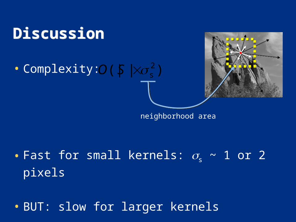
DiscussionDiscussion
• Complexity:
• Fast for small kernels: s ~ 1 or 2 pixels
• BUT: slow for larger kernels
)|(| 2sSΟ
neighborhood area
OutlineOutline
• Brute-force Implementation
• Separable Kernel [Pham and Van Vliet 05]
• Box Kernel [Weiss 06]
• 3D Kernel [Paris and Durand 06]
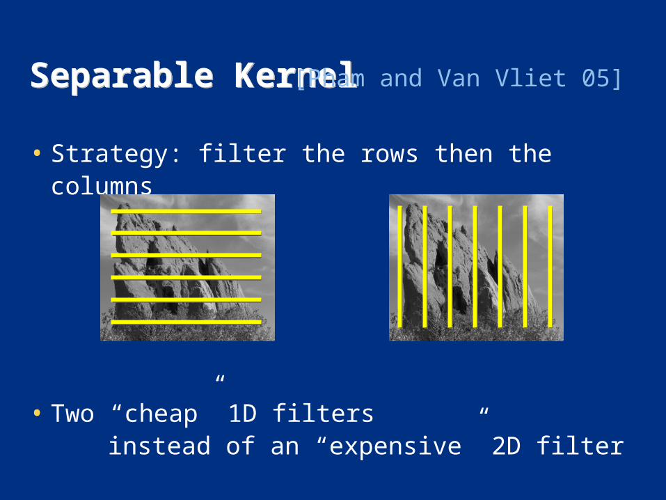
Separable KernelSeparable Kernel
• Strategy: filter the rows then the columns
• Two “cheap” 1D filters instead of an “expensive” 2D filter
[Pham and Van Vliet 05]
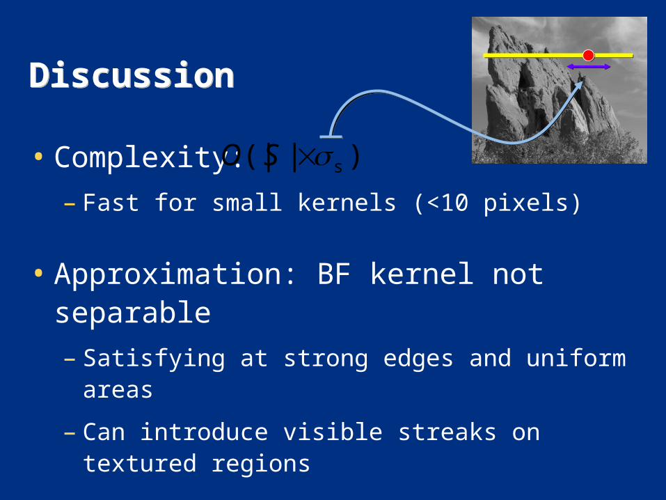
DiscussionDiscussion
• Complexity:
– Fast for small kernels (<10 pixels)
• Approximation: BF kernel not separable
– Satisfying at strong edges and uniform areas
– Can introduce visible streaks on textured regions
)|(| sSΟ

input
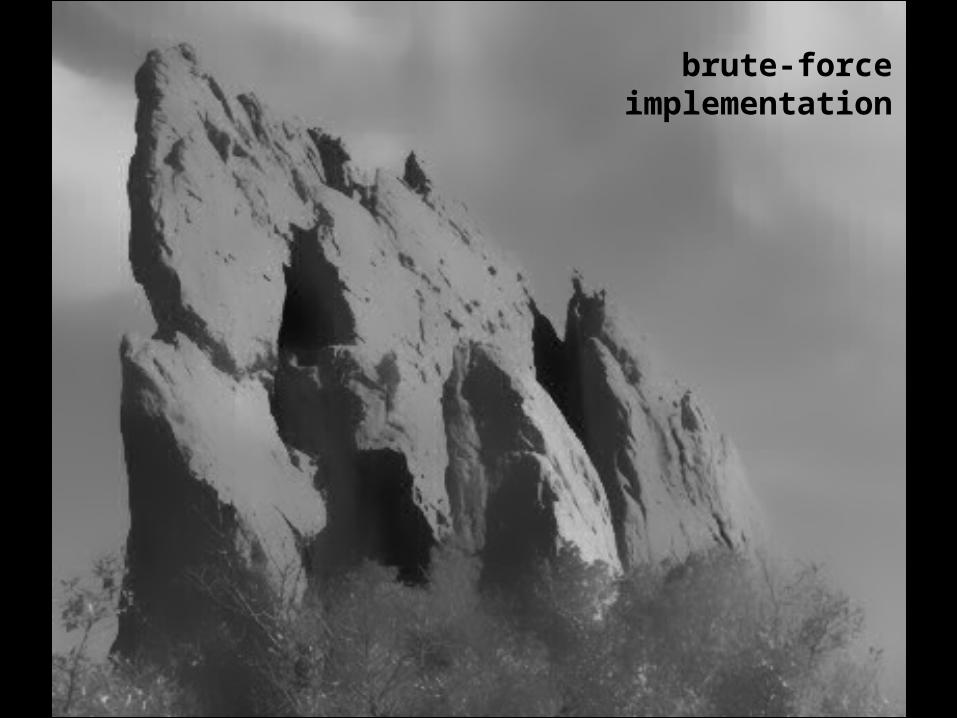
brute-forceimplementation
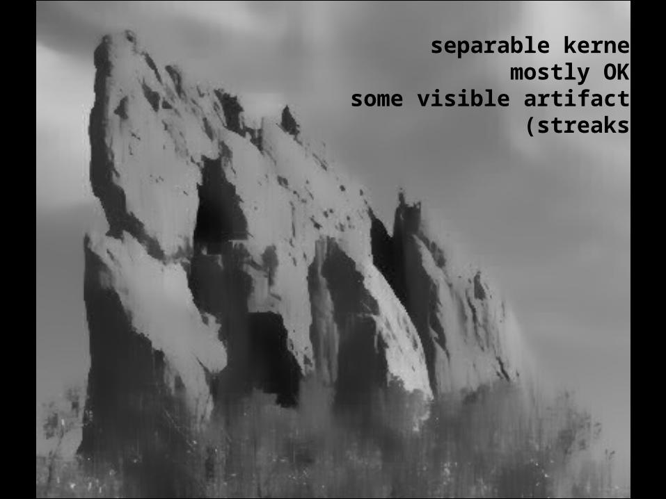
separable kernelmostly OK,
some visible artifacts(streaks)
OutlineOutline
• Brute-force Implementation
• Separable Kernel [Pham and Van Vliet 05]
• Box Kernel [Weiss 06]
• 3D Kernel [Paris and Durand 06]
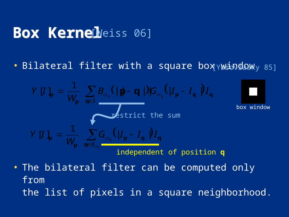
Box KernelBox Kernel
• Bilateral filter with a square box window
• The bilateral filter can be computed only from the list of pixels in a square neighborhood.
[Weiss 06]
S
IIIGBW
IYq
qqpp
p qp ||||||1
][rs
[Yarovlasky 85]
box window
s
r||
1][
B
IIIGW
IYq
qqpp
p
restrict the sum
independent of position q
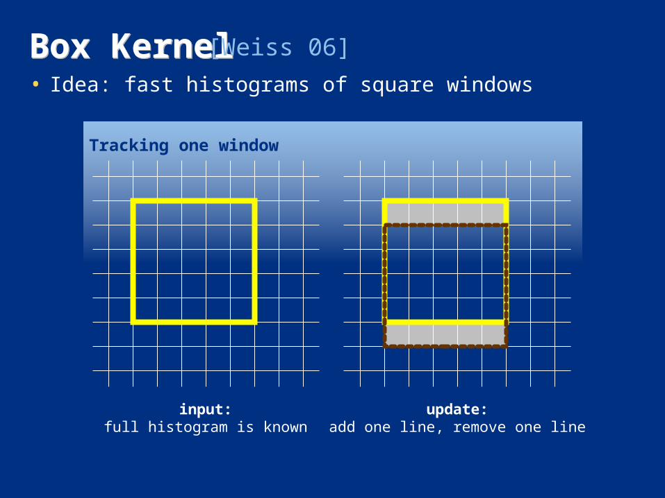
Box KernelBox Kernel• Idea: fast histograms of square windows
[Weiss 06]
input:full histogram is known
update:add one line, remove one line
Tracking one window
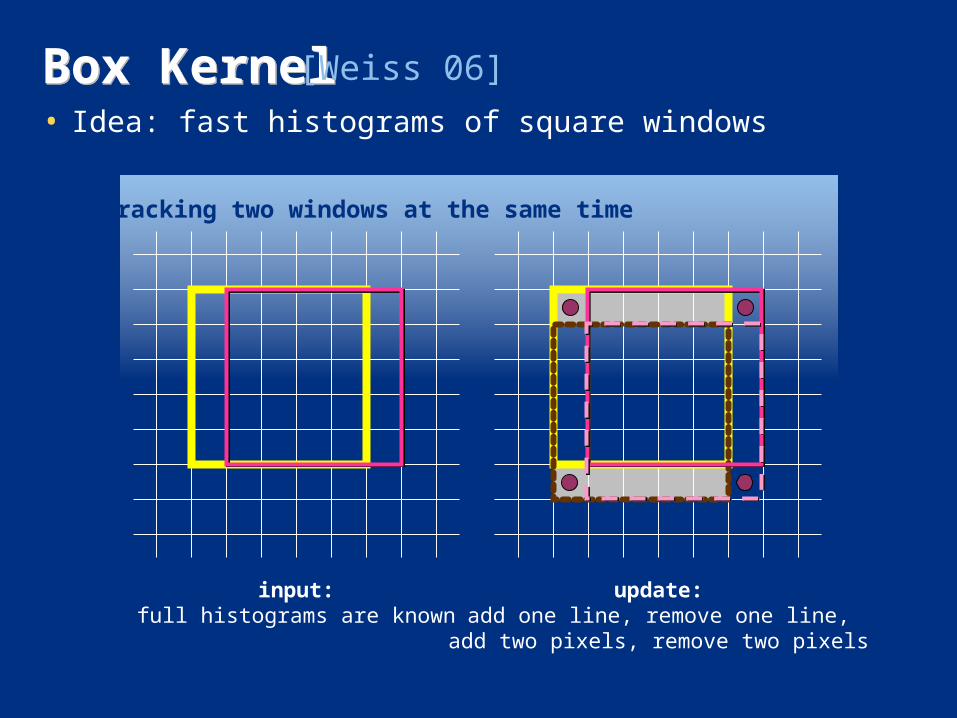
Box KernelBox Kernel• Idea: fast histograms of square windows
[Weiss 06]
input:full histograms are known
update:add one line, remove one line,
add two pixels, remove two pixels
Tracking two windows at the same time
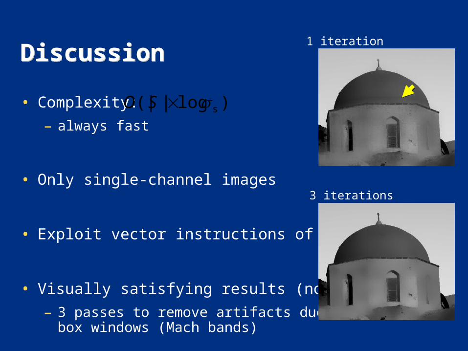
DiscussionDiscussion
• Complexity:
– always fast
• Only single-channel images
• Exploit vector instructions of CPU
• Visually satisfying results (no artifacts)
– 3 passes to remove artifacts due to box windows (Mach bands)
)log|(| sSΟ
1 iteration
3 iterations

input

brute-forceimplementation
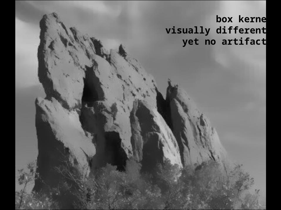
box kernelvisually different,
yet no artifacts
OutlineOutline
• Brute-force Implementation
• Separable Kernel [Pham and Van Vliet 05]
• Box Kernel [Weiss 06]
• 3D Kernel [Paris and Durand 06]
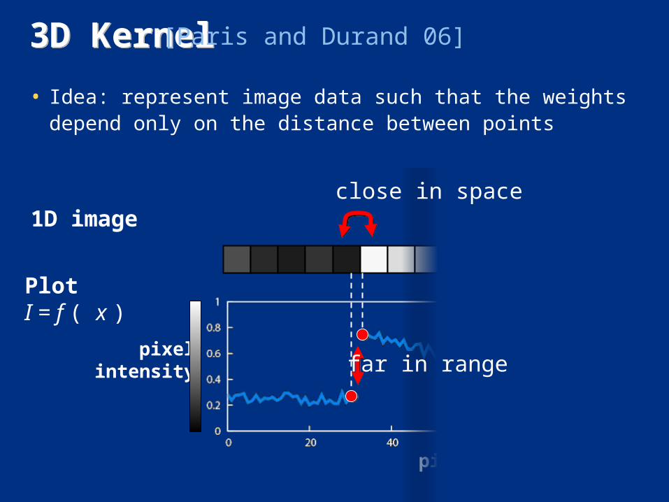
3D Kernel3D Kernel
• Idea: represent image data such that the weights depend only on the distance between points
[Paris and Durand 06]
pixelintensity
pixel position
1D image
PlotI = f ( x )
far in range
close in space
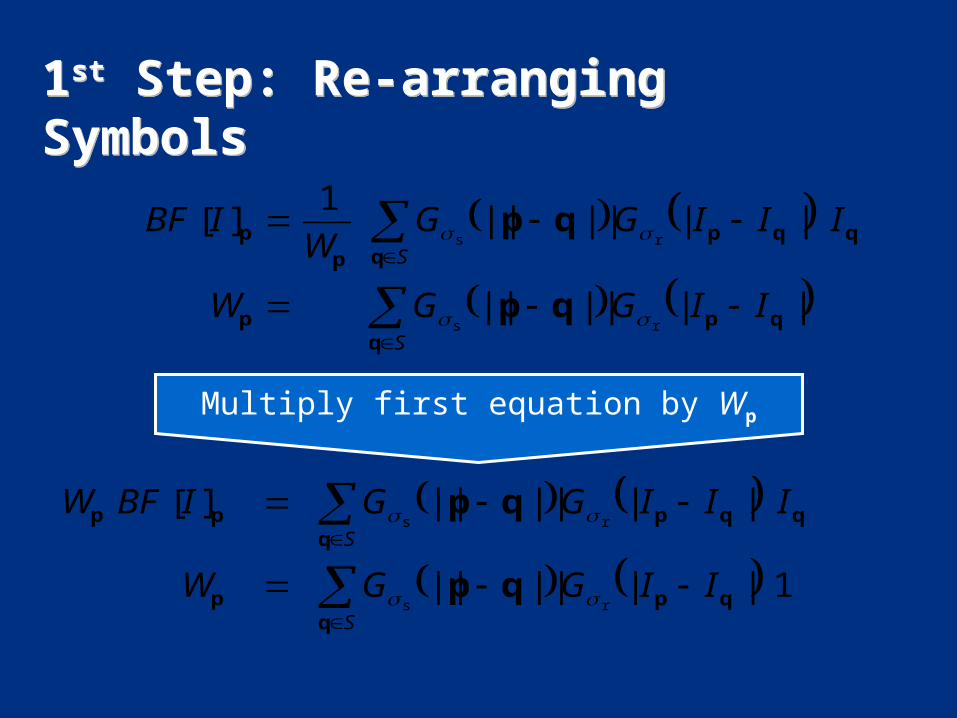
1st Step: Re-arranging Symbols1st Step: Re-arranging Symbols
S
S
IIGGW
IIIGGW
IBF
qqpp
qqqp
pp
qp
qp
||||||
||||||1
][
rs
rs
1||||||
||||||][
rs
rs
S
S
IIGGW
IIIGGIBFW
qqpp
qqqppp
qp
qp
Multiply first equation by Wp
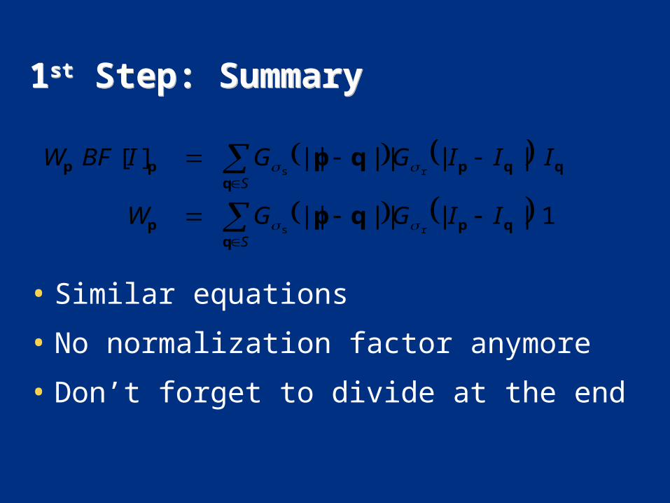
1st Step: Summary1st Step: Summary
• Similar equations
• No normalization factor anymore
• Don’t forget to divide at the end
1||||||
||||||][
rs
rs
S
S
IIGGW
IIIGGIBFW
qqpp
qqqppp
qp
qp
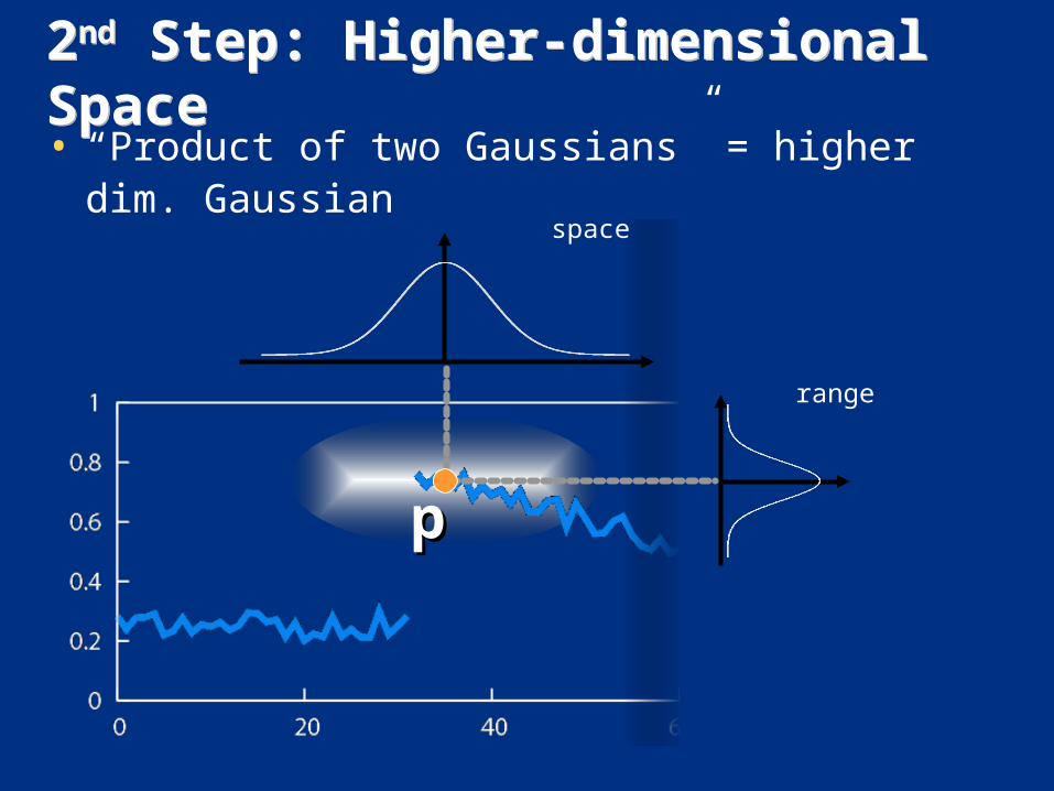
2nd Step: Higher-dimensional Space2nd Step: Higher-dimensional Space
pp
space
range
• “Product of two Gaussians” = higher dim. Gaussian
2nd Step: Higher-dimensional Space2nd Step: Higher-dimensional Space
pp
space
range
• 0 almost everywhere, I at “plot location”
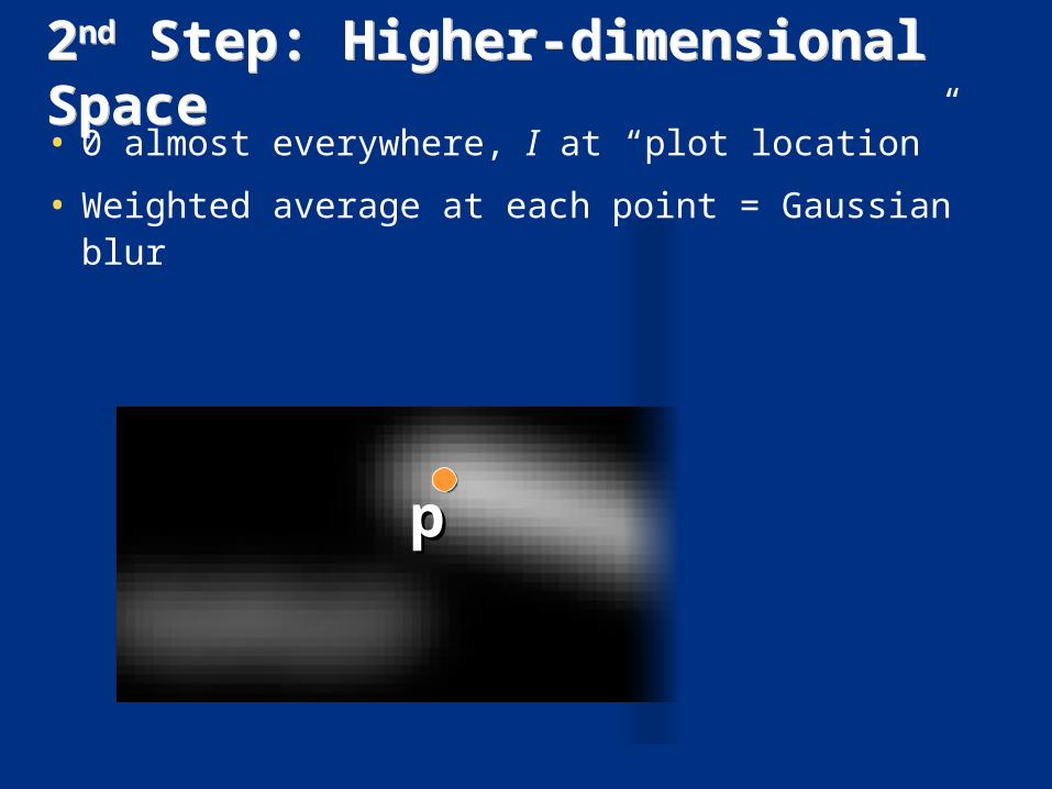
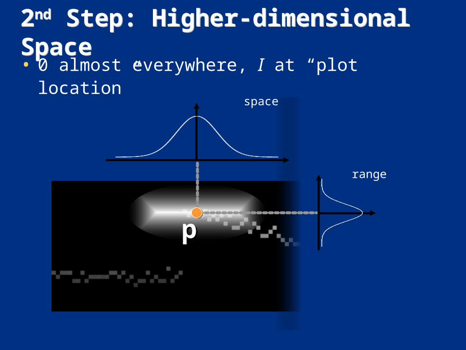
2nd Step: Higher-dimensional Space2nd Step: Higher-dimensional Space
pp
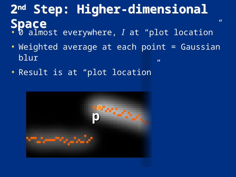
• 0 almost everywhere, I at “plot location”
• Weighted average at each point = Gaussian blur
2nd Step: Higher-dimensional Space2nd Step: Higher-dimensional Space
pp
• 0 almost everywhere, I at “plot location”
• Weighted average at each point = Gaussian blur
• Result is at “plot location”
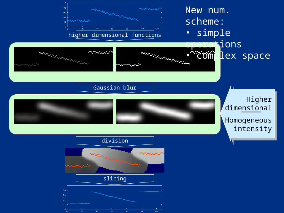
higher dimensional functions
Gaussian blur
division
slicing
Higherdimensional
Homogeneousintensity
Higherdimensional
Homogeneousintensity
New num. scheme:• simple operations• complex space
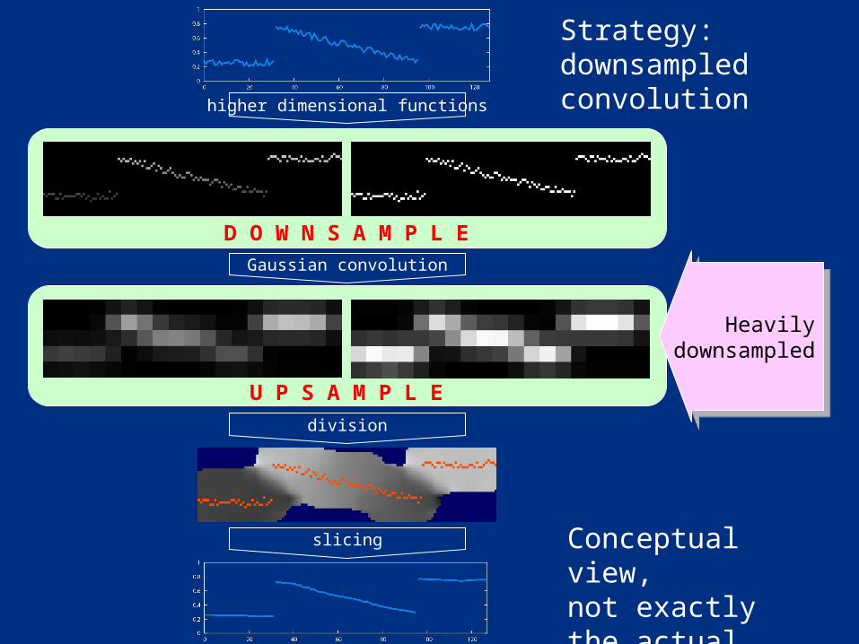
higher dimensional functions
Gaussian convolution
division
slicing
D O W N S A M P L E
U P S A M P L E
Heavilydownsampled
Heavilydownsampled
Strategy:downsampledconvolution
Conceptual view,not exactly the actual algorithm
Actual AlgorithmActual Algorithm
• Never compute full resolution
– On-the-fly downsampling
– On-the-fly upsampling
• 3D sampling rate = ),,( rss
Pseudo-code: StartPseudo-code: Start
• Input
– image I
– Gaussian parameters s and r
• Output: BF [ I ]
• Data structure: 3D arrays wi and w (init. to 0)

Pseudo-code: On-the-fly Downsampling
Pseudo-code: On-the-fly Downsampling
• For each pixel
– Downsample:
– Update:
SYX ),(
rss
),(,,),,(
YXIYX
zyx
1),,(
),(),,(
zyxw
YXIzyxwi
D O W N S A M P L E
U P S A M P L E
[ ] = closest int.
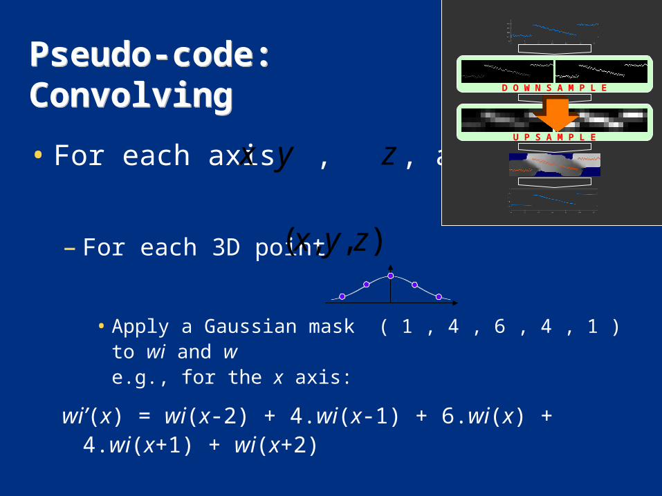
Pseudo-code: ConvolvingPseudo-code: Convolving
• For each axis , , and
– For each 3D point
• Apply a Gaussian mask ( 1 , 4 , 6 , 4 , 1 ) to wi and we.g., for the x axis:
wi’(x) = wi(x-2) + 4.wi(x-1) + 6.wi(x) + 4.wi(x+1) + wi(x+2)
x
y
z
),,( zyx
D O W N S A M P L E
U P S A M P L E
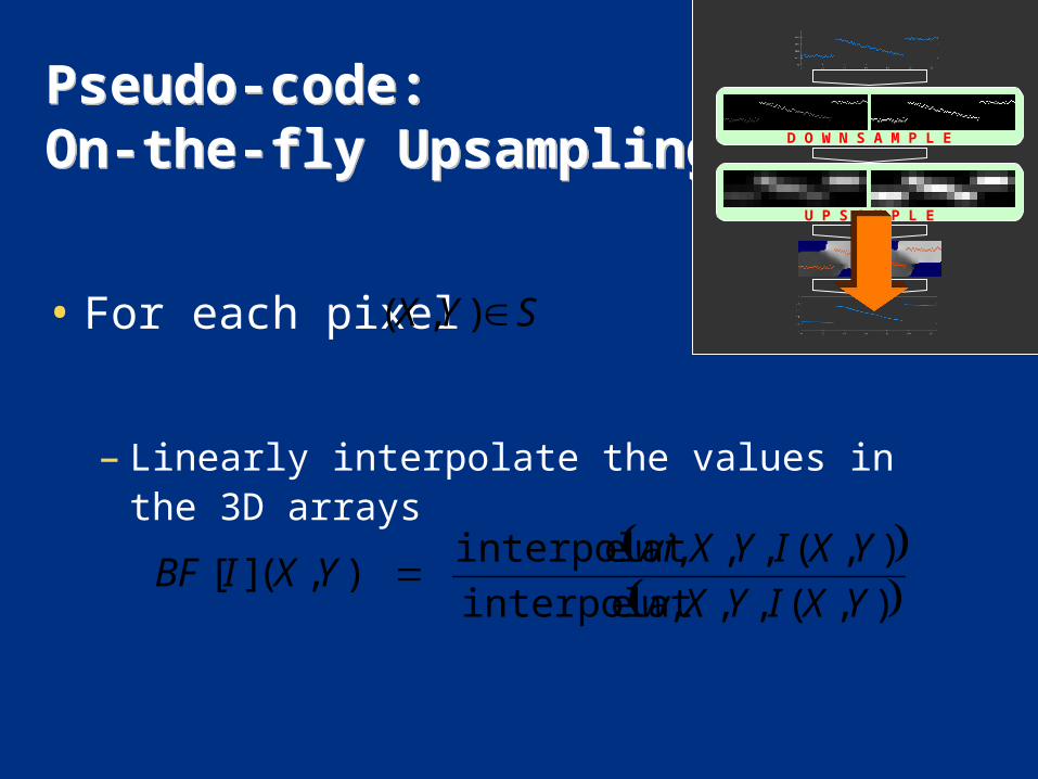
Pseudo-code: On-the-fly UpsamplingPseudo-code: On-the-fly Upsampling
• For each pixel
– Linearly interpolate the values in the 3D arrays
SYX ),(
),(,,,einterpolat
),(,,,einterpolat),(][
YXIYXw
YXIYXwiYXIBF
D O W N S A M P L E
U P S A M P L E
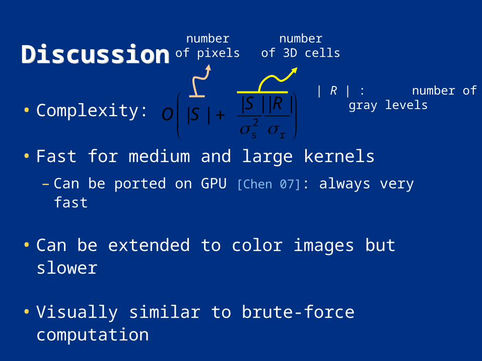
DiscussionDiscussion
• Complexity:
• Fast for medium and large kernels
– Can be ported on GPU [Chen 07]: always very fast
• Can be extended to color images but slower
• Visually similar to brute-force computation
r2s
||||||
RS
SΟ
numberof pixels
numberof 3D cells
| R | : number of gray levels
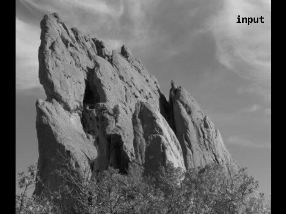
input

brute-forceimplementation

3D kernelvisually similar
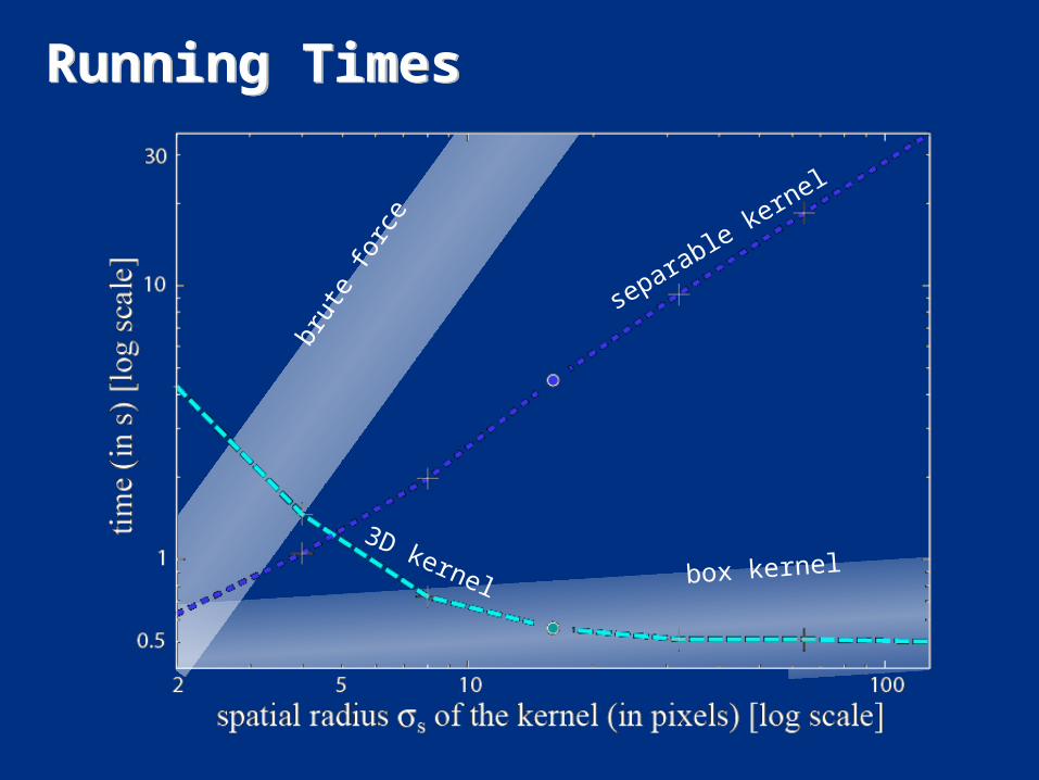
Running TimesRunning Times
separable kernel
3D kernel box kernel
brut
e fo
rce
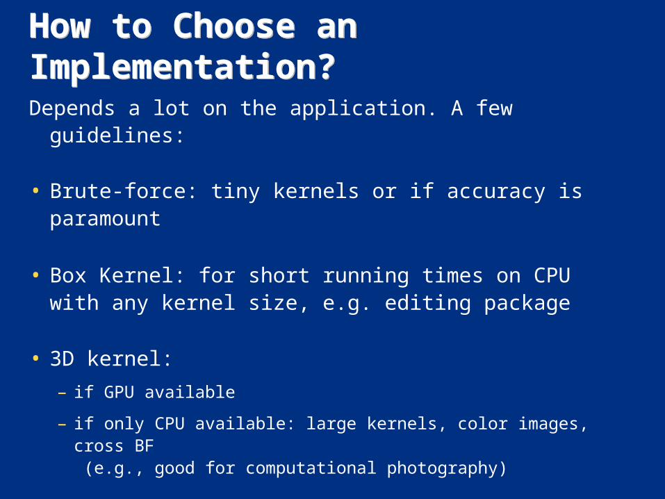
How to Choose an Implementation?How to Choose an Implementation?
Depends a lot on the application. A few guidelines:
• Brute-force: tiny kernels or if accuracy is paramount
• Box Kernel: for short running times on CPU with any kernel size, e.g. editing package
• 3D kernel:
– if GPU available
– if only CPU available: large kernels, color images, cross BF (e.g., good for computational photography)

Questions ?Questions ?