course notes set 1

8/7/2019 Course Notes Set 1

http://slidepdf.com/reader/full/course-notes-set-1 1/27

1

Maxwell’s Equations in Differential Form

d cii

id i

J J J t D

E J H

M M M t B

E

vvvv

vvv

rrrv

v

++=∂∂++=×∇

−−=−∂∂−=×∇

σ

mv

ev

B

D

ρ

ρ

=⋅∇

=⋅∇v

v

t B

M d ∂∂=

vv

, E J cvv

σ = ,t D

J d ∂∂=

vv

≡E

v

Electric field intensity [V/m]

≡Bv

Magnetic flux density [Weber/m 2 = V s/m 2 = Tesla]

≡iM

v

Impressed (source) magnetic current density [V/m 2]

≡d M

v

Magnetic displacement current density [V/m 2]

≡H v

Magnetic field intensity [A/m]

≡iJ

v

Impressed (source) electric current density [A/m 2]

≡Dv

Electric flux density or electric displacement [C/m 2]

≡cJ

v

Electric conduction current density [A/m 2]

≡d J

v

Electric displacement current density [A/m 2]

≡evρ Electric charge volume density [C/m 3]

≡

mvρ Magnetic charge volume density [Weber/m 3]

≡σ Electric conductivity [1/ Ω m]



2

Remarks:

1.

Impressed magnetic current density ( iM v

) and magnetic charge density ( mvρ ) areunphysical quantities introduced through “generalized” current to balanceMaxwell’s equations.

2. Although unphysical, iM v

, mvρ similar to iJ v

and evρ can be considered as energysources that generate the fields.

3.

Through “equivalent principle” iM

v

and mvρ can be used to simplify the solutionsto some boundary value problems.

4. t

BM d ∂

∂=v

v

(magnetic displacement current density [V/m 2]) is introduced

analogous tot D

J d ∂∂=

vv

(electric displacement current density [A/m 2])

iJ

v

Current source

cJ v

dt

DJ d

vv ∂=

iJ v

generates the electricdisplacement current



3

Integral form of Maxwell’s Equations

Elementary vector calculus:

Stokes’ Theorem: ( ) ∫ ∫∫ ⋅=⋅×∇C S

ld Asd Avvvv

• It says that if you want to know what is happening in the interior of a surface boundedby a curve just go around the curve and add up the field contributions.

Divergence Theorem: ( ) ∫∫ ∫∫∫ ⋅=⋅∇

SV

sd AdV Avvv

• In simple words, divergence theorem states that if you want to know what is happeningwithin a volume of V just go around the surface S (bounding volume V ) and add up thefield contributions. Null Identities:

( )( ) φ φ −∇=⇔=×∇⇔=∇×∇

×∇=⇔=⋅∇⇔=×∇⋅∇

E E

ABBAvv

vvvv

atic)(electrost00

00

• The Divergence and Stokes’ theorems can be used to obtain the integral forms of theMaxwell’s Equations from their differential form.

•

∫∫ ∫∫ ∫∫ ⋅−⋅

∂

∂−=⋅×∇⇒−∂

∂−=×∇S

iSS

i sd M sd Bt

sd E M t

BE

vvvvvvvv

v

S

volume V

surface S

C



4

∫∫ ∫∫ ∫ ⋅−⋅∂∂−=⋅⇒

S

i

SC

sd M sd Bt

ld E vvvvvv

• ∫∫ ∫∫ ∫∫ ∫∫ ⋅+⋅+⋅∂∂=⋅×∇⇔++

∂∂=×∇

S

i

SSS

i sd J sd E sd t D

sd H J E t D

H vvvvv

v

vvvvv

v

σ σ

∫∫ ∫∫ ∫∫ ∫ ⋅+⋅+⋅∂∂=⋅⇒

Si

Sc

SC

sd J sd J sd Dt

ld H vvvvvvvv

Where E J cvv

σ =

• e

V

ev

SV

ev

V

ev Qdvsd DdvdvDD ==⋅⇒=⋅∇⇔=⋅∇ ∫∫∫ ∫∫ ∫∫∫ ∫∫∫ ρ ρ ρ vvvv

• ∫∫∫ ∫∫ ∫∫∫ ∫∫∫ ==⋅⇒=⋅∇⇔=⋅∇

V

mvm

V

mv

V

mv dvQsd BdvdvBB ρ ρ ρ vvv

Since 00 =⋅⇒= ∫∫ S

m sd BQvv

S

C

S

V



5

Helmholtz Theorem

• Traditionally, Newtonian mechanic is formulated in terms of force ( F r

) and torque ( τ r

),

,dt Pd

F

rr

= dt Ld r

r

=τ where Lr

is the angular momentum.

However such an approach to classical electromagnetism will be unnecessarilycumbersome. Instead, the description of electromagnetics starts with Maxwell’sequations which are written in terms of curls and divergences. The question is thenwhether or not such a description (in terms of curls and divergences) is sufficient andunique? The answer to this question is provided by Helmholtz Theorem • A vector field is determined to within an additive constant if both its divergence and itscurl are specified everywhere.

• Equivalent statement: A vector field is uniquely specified by giving its divergence andits curl within a region and its normal component over the boundary, that is if:S and C

v

are known and given bySM =⋅∇

v

,C M

vv

=×∇ and nM

v

(the normal component of M v

on the boundary) is also known; then M v

isuniquely defined. Remark: Helmholtz’s theorem allows us to appreciate the importance of the Maxwell’sequations in which E

v

and H v

are defined by their divergence and curl.

Ex.: Bt

E vv

∂∂−=×∇ andε

ρ evE =⋅∇

v

Irrotational & Solenoidal Fields (Use of HelmholtzTheorem)

Definition:• A field is irrotational if its curl is zero

ii F F ≡=×∇ 0v

is irrotational

• A field is solenoidal (divergenceless) if its divergence is zeross F F

vv

≡=⋅∇ 0 is solenoidal Theorem:• A vector field which its divergence and curl vanishes at infinity can be written as thesum of an irrotational & a solenoidal fields.



6

• According to the theorem stated above, the vector field M v

can be written as

si F F M vvv

+= (1) • Since iF

v

is irrotational then φ −∇=⇒=×∇ii F F

vv

0 where φ is a scalar function.

• Since sF

v

is solenoidal then AF F ss

vvv

×∇=⇒=⋅∇ 0 then (1) AM

vv

×∇+−∇=⇒ φ

Constitutive Relations

E Dvv

ε =

0

0

μ μ μ

ε ε ε

μ

r

r

H B

===

vv

≡ε permittivity [F/m]≡

oε vacuum permittivity = 8.85 ×10 -12 [F/m]

≡r ε Relative permittivity or dielectric constant [#]≡μ permeability [H/m]≡

0μ free space permeability = 4 π × 10 -7 [H/m]≡

r μ relative permeability [#] • We also write

mr χ μ += 1 (1)

er χ ε +=1 (2)Where mχ and eχ are the magnetic and electric susceptibility, respectively. mχ , eχ aredimensionless. • Index of refraction is defined as

r r n μ ε = (3)≡n index of refraction or phase index [#]

• If we are mostly concerned with non-magnetic materials then

r r n ε μ μ μ =⇒=⇒≈ 01

Polarization and Magnetization • Polarization vector P

v

and magnetization vector M v

are related to Dv

and E v

andBv

and H v

according to:



7

( )M H M H B

E PDvvvvv

vvv

+=+=+=

000

0

)5(

(4)

μ μ μ

ε

• Assuming E P e

vv

χ ε 0= , then:

( )E D

E E E E PE D r eevv

vvvvvvv

ε ε ε χ ε χ ε ε ε

=⇒=+=+=+= 00000 1

• Assuming H M m

vv

χ = then

( )H B

H H M H B r omvv

vvvvv

μ

μ μ χ μ μ μ

=⇒=+=+= 1000

• ε and μ describe the macroscopic response of the media. ε characterizes the electricresponse while μ describes the magnetic response. In the following we assume our

medium is nonmagnetic.

Homogeneous vs. Inhomogeneous, Isotropic vs.Anisotropic, Linear vs. Non-Linear • If ε depends on position, i.e. ( )r ε , media is non-homogeneous.

• If ε depends on the direction of the applied field, i.e., Dv

and E v

are not co-linear, then themedium is said to be anisotropic.• In the case of anisotropic medium ε is a tensor (for our purposes a matrix of rank 2).

We then write:E Dv

ε = (1) where

⎥

⎥

⎥

⎦

⎤

⎢

⎢

⎢

⎣

⎡

⎥

⎥

⎥

⎦

⎤

⎢

⎢

⎢

⎣

⎡

=⎥

⎥

⎥

⎦

⎤

⎢

⎢

⎢

⎣

⎡

z

y

x

zzzyzx

yzyyyx

xzxyxx

z

y

x

E

E

E

D

D

D

ε ε ε

ε ε ε

ε ε ε

ε 0 (2)

• If ε depends on the magnitude of the applied field, i.e. ( )E v

ε , we say medium is

nonlinear. Note that in this case even though permittivity is a function of the filedstrength, it can still be a scalar function. • An example of non-linear medium is when

( )2/1

2222

0

11 )3(

−

⎥⎦

⎤

⎢⎣

⎡ −+= E Bcbε

ε ,

Where b is the maximum field strength.



8

• Interesting thing about (3) is the fact that it describes the response of the vacuum,(proposed by Born & Infeld) in order to address the problem of vacuum infinite self-energy.

Infinite Self Energy• A charge particle can be thought as the localization of the charge density. As a chargedistribution localizes to a point charge, its electromagnetic energy grows more and moreand becomes unbounded. To avoid this infinite self-energy we can think that somesaturation of field strength takes place, i.e., field strength has an upper bound. This

classical non-linear effect is given by ( )2/1

2222

0

11 ⎥

⎦

⎤

⎢⎣

⎡ −+= E Bcbε

ε

• However, there are few problems with Born & Infeld classical non-linear vacuumresponse. (1) The theory suffers from arbitrariness in the manner in which thenonlinearities occur. (2) There are problems with transitions to the quantum domain. (3)

So far, there has been no experimental evidence of the existence of this kind of classicalnonlinearities.• As to the last point, we may note that in the orbits of electrons in atoms, field strengthsof 10 11-10 17 V/m are present. For heavier atoms, these fields can be even as large as1021 V/m at the edge of the nucleus; yet ordinary quantum theory with linear superposition is sufficient to describe the observed phenomena with a high degree of accuracy.

HW: Consider a hydrogen atom unexcited and in thermal equilibrium. Calculate themagnitude of the electric field due to its nucleus at the site of its electron.

Temporal dispersion • If ε depends on frequency, i.e. ( )ω ε , we say the medium is dispersive (frequencydispersion)

220

2

0

1 )1(ω ω γ ω

ω

ε ε

ε −+

+==j

pr

• Note that from (1) we can writeε ε ε ′′−′= j )2(

• Remarks: Temporal dispersion means that the parameters describing the mediumresponse (e.g. ε and μ ) are functions of time derivatives. Spatial dispersion means thatthe parameters describing the medium response (e.g. ε and μ ) are functions of spacederivatives.• If a medium is linear, homogeneous, and isotropic, we say the medium is simple.

Electric Field• Electric field due to a point charge in origin



9

x

y

A r v

r a

1q

Observation Pointz3

0

13

0

12

0

1

44

ˆ

4 r r q

r

r q

r

aqE r

v

v

v

v

v

πε πε πε === where

r r

r r

a r

v

v

v

==ˆ and we use the shorthand

notation r r =v

. • Electric filed due to a point charge not at the origin

30

13

0

12

0

1

44ˆ

4 r r

r r q

R

Rq

R

aqE R

′−′−===

vv

vv

v

v

v

v

πε πε πε

• Superposition principle

( ) ( ) ( )⎥

⎥

⎦

⎤

⎢

⎢

⎣

⎡+

′−′−+

′−′−+

′−′−=

⎥

⎥

⎦

⎤

⎢

⎢

⎣

⎡

+++=

⎥

⎥

⎦

⎤

⎢

⎢

⎣

⎡

+++=

Lvv

vv

vv

vv

vv

vv

Lv

v

v

v

v

v

Lvvv

v

3

3

333

2

223

1

11

0

3

3

333

2

223

1

11

0

2

3

332

2

222

1

11

0

41

41

ˆˆˆ4

1

r r

r r q

r r

r r q

r r

r r q

R

Rq

R

Rq

R

Rq

R

aq

R

aq

R

aqE RRR

πε

πε

πε

∑= ′−

′−=N

k k

k k

r r

r r qE

13

041

vv

vv

πε

Electric Field & Potential due to Continuous ChargeDistribution• Volume charge density, ( ) ( )zyxr vv

′′′′=′′ ,,ρ ρ v

x

y

z A

r v

r ′v

1qv

r r R ′−=vvv

x

y

z

1r ′v

2r ′v

3r ′v

1qv

2qv

3qv

A

1Rv

2Rv

3R

v

r v

Observation Point

Observation Point



10

x

y

z

r r R ′−= vvv

r v

r ′v Differentialline charge lρ ′

x

y

z

r v ′

r v

r r R ′−= vvv

Differentialsurface chargedensity sρ ′

A (Observation point)

∫∫∫ ′

′′′−′−=

′′′−′−=

′′=

vv

v

v

vd r r

r r E

vd r r

r r E d

vd R

RE d

ρ πε

ρ πε

ρ πε

30

30

30

41

41

4

1

vv

vvv

vv

vvv

v

vv

∫∫∫ ∫∫∫ ∫∫∫ ′ ′′ ′−

′′=

′′=

′′=

v v

v

v

vv

r r vd

Rvd

Rvd

V vvvρ

πε ρ

πε ρ

πε 000 41

41

41

HW: From the above can you guess what forms the potentials due to a single or a

collection of charges must have. • Surface charge density, ( ) ( )zyxr ss

′′′′=′′ ,,ρ ρ v

sd r r

r r sd

R

Rsd

R

aE s

ss

sss

R ′′′−′−=′′=′′= ∫∫ ∫∫ ∫∫

′′′ρ

πε ρ

πε ρ

πε 30

30

20 4

14

1ˆ4

1vv

vv

v

v

v

v

∫∫ ∫∫ ∫∫ ′′′ ′−

′′=′′=′′=s

s

s

s

s

s

r r sd

Rsd

Rsd

V vvvρ

πε ρ

πε ρ

πε 000 41

41

41

• E

v

and V due to a line charge, ( ) ( )zyxr ll′′′′=′′ ,,ρ ρ

v

x

y

z A (Observation point)

Differentialvolume chargedensity vρ ′

r ′v

r v

r r R ′−= vvv



11

ld r r

r r ld

R

Rld

R

aE l

ll

lll

R ′′′−′−=′′=′′= ∫ ∫ ∫

′′′ρ

πε ρ

πε ρ

πε 30

30

20 4

14

1ˆ4

1vv

vv

v

v

v

v

∫ ∫ ∫ ′′ ′ ′−

′′=

′′=

′′=

l

l

l l

ll

r r ld

Rld

Rld

V vvvρ

πε ρ

πε ρ

πε 000 41

41

41

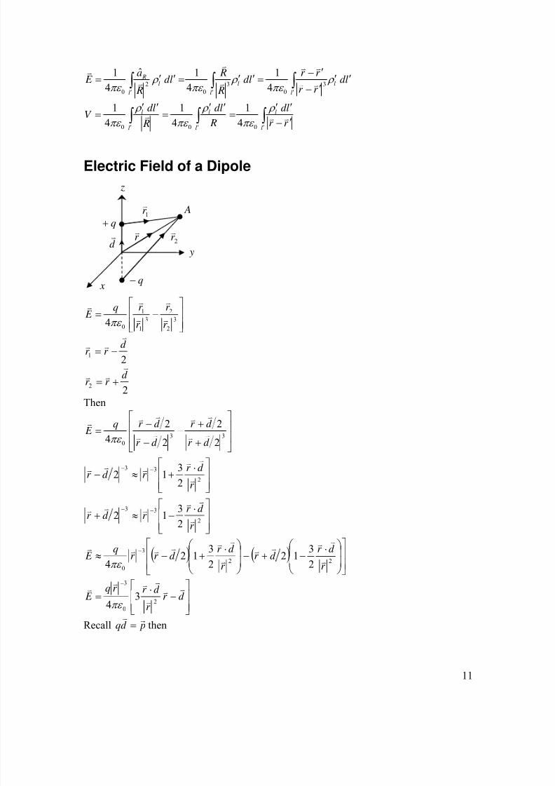
Electric Field of a Dipole

2

2

4

2

1

32

23

1

1

0

d r r

d r r

r

r

r

r qE

v

vv

v

vv

v

v

v

vv

+=

−=

⎥

⎥

⎦

⎤

⎢

⎢

⎣

⎡

−=πε

Then

⎥

⎥

⎦

⎤

⎢

⎢

⎣

⎡ ⋅−≈+

⎥

⎥

⎦

⎤

⎢

⎢

⎣

⎡ ⋅+≈−

⎥

⎥

⎦

⎤

⎢

⎢

⎣

⎡

+

+−−

−=

−−

−−

2

33

2

33

330

23

12

23

12

2

2

2

24

r

d r r d r

r

d r r d r

d r

d r

d r

d r qE

v

vvvvv

v

vvvvv

vv

vv

vv

vv

v

πε

( ) ( ) ⎥⎥

⎦

⎤

⎢⎢

⎣

⎡

⎟⎟

⎠

⎞

⎜⎜

⎝

⎛ ⋅−+−

⎟⎟

⎠

⎞

⎜⎜

⎝

⎛ ⋅+−≈ −

223

0 2312

2312

4 r d r d r

r d r d r r qE

v

vvv

v

v

vvv

vvv

πε

⎥

⎥

⎦

⎤

⎢

⎢

⎣

⎡

−⋅=−

d r r

d r r qE

vv

v

vvvv

20

3

34πε

Recall pd qrv

= then

x

y

z

q+

q−

d v

r v

1r v

2r v

A



12

( )⎥

⎥

⎦

⎤

⎢

⎢

⎣

⎡−⋅= pr

r

pr

r E

rv

v

rv

v

v

230

3

4

1

πε

• For our coordinate system zapp ˆ=r

• r v

is the position vector in spherical coordinate, then let us express E v

in the sphericalcoordinate

( ) ( ) ( )( ) ( ) ( )

θ φ θ

φ θ

φ φ

θ φ θ φ θ

θ φ θ φ θ

φ θ φ θ φ θ

φ

θ

φ φ θ θ

cossinsin

cossin

0cossin

sinsincoscoscos

cossinsincossin

ˆ,,ˆ,,ˆ,,

ˆ,,ˆ,,ˆ,,

r zr y

r x

A

A

A

A

A

A

azyxAazyxAazyxAA

ar Aar Aar AA

z

y

zr

zzyyxx

r r

==

=

⎥

⎥

⎥

⎦

⎤

⎢

⎢

⎢

⎣

⎡

⎥

⎥

⎥

⎦

⎤

⎢

⎢

⎢

⎣

⎡

−−=

⎥

⎥

⎥

⎦

⎤

⎢

⎢

⎢

⎣

⎡

++=

++=v

v

with

( )paaappp

p

p

p

p

r zz

zr

θ

φ

θ θ θ θ

θ ˆsinˆcosˆ

0

sin

cos−==⇒

⎥

⎥

⎥

⎦

⎤

⎢

⎢

⎢

⎣

⎡

−=⎥

⎥

⎥

⎦

⎤

⎢

⎢

⎢

⎣

⎡

r

• Or finally from

( )⎥

⎥

⎦

⎤

⎢

⎢

⎣

⎡−⋅= pr

r

pr

r E

rv

v

rv

v

v

230

3

4

1

πε

we get

( ) ( )⎥

⎥

⎦

⎤

⎢

⎢

⎣

⎡−−−⋅= paaar

r

paaar

r E r r

r r θ

θ θ θ θ θ

πε ˆsinˆcosˆ

ˆsinˆcosˆ314

123

0vv

v

⇒

[ ]θ θ θ πε

aar

pE r ˆsinˆcos2

43

0

+=v

v

, where r r =r

HW: Show that potential at point A for an electric dipole is given by

20

20

4ˆ

4

ˆr

ap

r

apV r r

πε πε

⋅=⋅=r

v

r

r v

q+

q−

A

d



13



14

Electric Polarization Pv

v

pP

vN

k k

v ′Δ= ∑

′Δ

=→′Δ

1

0limt

r

v

pr

[C·m] Electric dipole moment

Pr

[C/m 2] Electric polarization vector N [#/m 3] is the number of dipoles per unit volume • P

r

[C/m 2] is the volume density of electric dipole moment pr

[C·m]

Note Pr

and Dv

have the same units [C/m 2]: PE Dvvv

+= 0ε

• Polarization vector Pr

may come to exist due to (a) induced dipole moment, (b)alignment of the permanent dipole moments, or (c) migration of ionic charges.

• In differential form:vd pd

P ′=

rr

Potential due to Bound (Polarized) Surface & VolumeCharge Densities

A dielectric of volume v′ is polarized. We want to calculate the potential V [Volt] set upby this polarized dielectric.

• Potential due to a single dipole

204ˆR

apV R

πε

⋅=r

x

y

z

r ′v

r v

A

Rv

Differential volumeelement vd ′

v′



15

x

y

z

source ( )zyx ′′′ ,,

( )zyxA ,,

R

• An elemental electric dipole, having a differential electric dipole moment of pd r

[C·m],

will set up a differential potential 204ˆRapd

dV R

πε

⋅=r

But from our definition of polarization we ⇒′= vd Ppd rr

vd R

aPRapd dV RR ′⋅=⋅= 2

02

0 4ˆ

4ˆ

πε πε

rr

Total potential V is found by integrating the above:

vd R

aPV

v

R ′⋅= ∫∫∫ ′

20

ˆ4

1r

πε

Where ( ) ( ) ( )22222 zzyyxxRR ′−+′−+′−==v

Note that 2

ˆ1R

aR

R=⎟⎠

⎞⎜⎝ ⎛

∇′ (see Remarks below) then

∫∫∫ ′ ′⎟⎠

⎞

⎜⎝ ⎛

∇′⋅=v

vd RPV 1

41

0

r

πε

Remarks: Few useful identities

( ) ( )RRf

aRf

RR

R

RaR

R

a

R

R

a

R

R

R

R

R

∂∂=∇

===∇

−=⎟⎠

⎞⎜⎝ ⎛ ∇

=⎟⎠

⎞⎜⎝ ⎛

∇′

ˆ

ˆ

ˆ1

ˆ1

2

2

v

v

v

( )RR

v

v32 4

1πδ =∇− , or ( )r r

r r ′−=

′−∇− vv

vv32 4

1πδ

and furthermore( ) ⇒∇′⋅+⋅∇′=⋅∇′ f AAf Af

vvv ( ) Af Af f Arvv

⋅∇′−⋅∇′=∇′⋅

* Let PArv

= andR

f 1= then

∫∫∫ ∫∫∫ ∫∫∫ ′ ′′′⎟⎠

⎞

⎜⎝ ⎛

⋅∇′−′⎟⎟⎠

⎞

⎜⎜⎝

⎛ ⋅∇′=′⎟⎠

⎞

⎜⎝ ⎛

∇′⋅v vv

vd PRvd RP

vd RPv

rr 11

Use divergence theorem ⇒

vd PR

sd RP

vd R

Pvv s

′⎟⎠

⎞⎜⎝ ⎛

⋅∇′−′⋅=′⎟⎠

⎞⎜⎝ ⎛

∇′⋅ ∫∫∫ ∫∫∫ ∫∫ ′′ ′

vrv

r 11

The potential then can be written as



16

⎥⎦

⎤

⎢⎣

⎡′⋅∇′

−′′⋅= ∫∫ ∫∫∫ ′S

n vd R

Psd

RaP

V

rr

ˆ4

1

0πε ,

Where na ′ˆ is perpendicular to surface S ′ bounding volume v′ .

Compare above to the previously obtained expressions for V due to surface and volumecharge densities, i.e.:

∫∫ ′

′′=

s Rsd

V ρ

πε 041

and ∫∫∫ ′

⇒′′

=v

v

Rvd

V ρ

πε 041

v

sn

P

aP

ρ

ρ

′=⋅∇′−

′=′⋅r

r

ˆ

Or in general, dropping the prim notation since we know that integration is carried withrespect to the prim coordinate, we define• Bound or polarized surface charge density: nsP aP ˆ⋅=

r

ρ [C/m 2]

• Bound or polarized volume charge PvP

r

⋅−∇=ρ [C/m3]

A polarized dielectric can be replaced by a bound (polarized) surface and volume chargedensities ( sPρ & vPρ ). The potential setup by these bound charges then can be calculated.

Generalized Gauss’ Law & Constitutive Relation E Dvv

ε =

• In free space0ε

ρ vE =⋅∇v

.

• When a medium is polarized we must take into account the effects of the bound charge,hence

( ) vv

vvpv

PE PE

PE

ρ ε ρ ε

ε ε ρ

ε

ρ

ε ρ

=+⋅∇⇒=⋅∇+⋅∇

⇒⋅∇−=+=⋅∇

rvrv

r

v

00

0000

Let’s define PE Dvvv

+= 0ε then

vD ρ =⋅∇v

← Generalized Gauss’ Law • Also note that for PE D

rvv

+= 0ε if E P e

vr

χ ε 0= then ( ) E E D r e

vvv

ε ε χ ε 00 1 =+=

Where er χ ε +=1 thenE E D r

vv

ε ε ε ==0 where r ε ε ε 0

=

Magnetization & Permeability



17

• Magnetic materials exhibit magnetic polarization ( M r

, magnetization) when subjectedto an applied magnetic field • This magnetization is the result of alignment of the magnetic dipoles of material withthe applied magnetic field. This is similar to electric polarization which is the result of

alignment of electric dipoles of the material with the applied electric field.

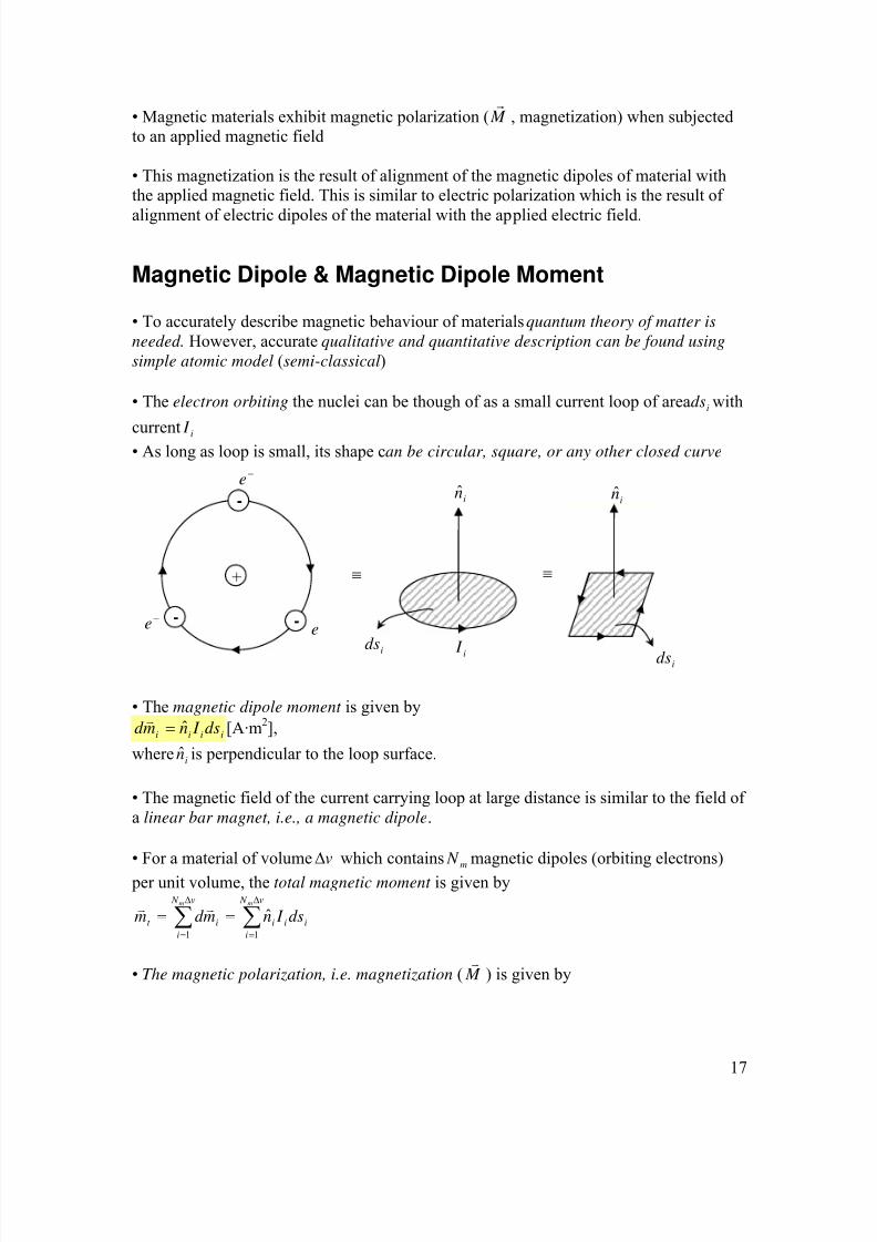
Magnetic Dipole & Magnetic Dipole Moment • To accurately describe magnetic behaviour of materials quantum theory of matter isneeded. However, accurate qualitative and quantitative description can be found usingsimple atomic model (semi-classical ) • The electron orbiting the nuclei can be though of as a small current loop of area ids with

current iI • As long as loop is small, its shape c an be circular, square, or any other closed curve

• The magnetic dipole moment is given by

iiii dsI nmd ˆ=v

[A·m 2],

where in is perpendicular to the loop surface. • The magnetic field of the current carrying loop at large distance is similar to the field of a linear bar magnet, i.e., a magnetic dipole . • For a material of volume vΔ which contains mN magnetic dipoles (orbiting electrons)per unit volume, the total magnetic moment is given by

∑∑Δ

=

Δ

=

==vN

iiii

vN

iit

mm

dsI nmd m11

ˆvv

• The magnetic polarization, i.e. magnetization ( M

v

) is given by

+

-

- - −e

−e

−e

in

iI ids

ids

≡ ≡

in



18

⎥⎦

⎤

⎢⎣

⎡

Δ=⎥⎦

⎤

⎢⎣

⎡

Δ=⎥⎦

⎤

⎢⎣

⎡

Δ= ∑∑

Δ

=→Δ

Δ

=→Δ→Δ

vN

iiii

v

vN

ii

vt

v

mm

dsI nv

md v

mv

M 10100

ˆ1limt

1limt

1limt

vvv

[A/m]

• Note that magnetization ( M

v

) is the volume density of the total magnetic dipole

moment ( t mv

), and also the fact that magnetization ( M

v

) has the same units as themagnetic field intensity , H

v

[A/m]. • In absence of an applied field ( 0=aB

v

) the magnetic dipoles point in random directions.

However, when 0≠aB

v

, the dipoles will experience a torque given by

iaiiaiaiiaiaiai BdsI BnBdsI Bmd Bmd Bmd Ψ=∠=∠=×=Δ sin),ˆsin(),sin(vvvvvvvvv

τ

• Subjected to the above torque, the magnetic dipoles realign themselves such that their moment ( imd

v

) is collinear with aBv

(see figure in the next page)

00 →Δ⇒→Ψ τ v

i Remark: Comparing the similarities between the torque & potential energy for electric &magnetic dipoles

aE

aB

E pd

Bmd vrr

vvr

×=Δ×=Δ

τ

τ

aE

aB

E pd U

Bmd U vr

vv

⋅−=Δ⋅−=Δ

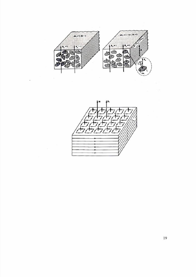
• From next page figure we see that in absence of an applied magnetic field , we can write

aa H Bvv

0 )1( μ = .

But, when a magnetic material is present, a magnetic polarization ( M v

) is also presentand an additional term must be added to (1). In order to take into account the influence of the material, we write

( )M H M H B aa

vvvv

+=+=000 )2( μ μ μ

• However, M

v

is ultimately related to the applied field aH v

. If we assume

am H M vv

χ = )3( ,

Where mχ is a scalar (or tensor) function then we have

[ ] aar am H H H Bvvv

μ μ μ χ μ ==+= 00 1 )4( ,

Where mr χ μ +=1 is the relative permeability and μ is the permeability .



19



20

Bound Magnetization Current Density• Recall that for an electric field applied to a medium we had

nsP aP ˆ⋅=r

ρ

PvP

r

⋅−∇=ρ , where Pr

is the electric polarization, vPρ and sPρ are the volume and

surface bound charges, and na is the normal to the surface. • Similarly, for magnetic field applied to a medium we have

nsm aM J ˆ×=vv

M J vm

vv

×∇=

• Here, smJ v

is the bound magnetization surface current density [A/m], vmJ v

is the bound

magnetization volume current density [A/m 2], and na is the normal to the surface.

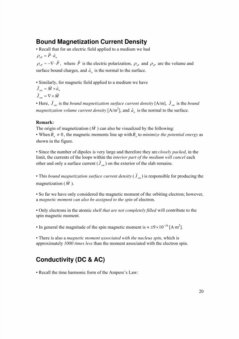
Remark:The origin of magnetization ( M

v

) can also be visualized by the following:• When 0≠

aBv

, the magnetic moments line up with aBv

to minimize the potential energy asshown in the figure. • Since the number of dipoles is very large and therefore they are closely packed , in thelimit, the currents of the loops within the interior part of the medium will cancel eachother and only a surface current ( smJ

v

) on the exterior of the slab remains.

• This bound magnetization surface current density ( smJ

v

) is responsible for producing themagnetization ( M

v

). • So far we have only considered the magnetic moment of the orbiting electron; however,a magnetic moment can also be assigned to the spin of electron. • Only electrons in the atomic shell that are not completely filled will contribute to thespin magnetic moment. • In general the magnitude of the spin magnetic moment is 24109 −×±≈ [A·m 2]. • There is also a magnetic moment associated with the nucleus spin , which isapproximately 1000 times less than the moment associated with the electron spin.

Conductivity (DC & AC) • Recall the time harmonic form of the Ampere’s Law:



21

E jE J J J J H siDC i

vvvvvvv

ωε σ ++=++=×∇ • Where ε in general is complex: ε ε ε ′′−′= j and sσ is the static (DC ) conductivity (thisis due to free carriers; i.e., electrons at 0=ω ). • The Ampere law then can be written as:

( ) ( ) E jE J E jE J E jjE J H eisisi

vvvvvvvvvv

ε ω σ ε ω ε ω σ ε ε ω σ ′++=′+′′++=′′−′++=×∇ where we have defined the followings:

≡′′+= ε ω σ σ se Equivalent (effective ) conductivit y [1/ Ω ·m]≡′′= ε ω σ a Alternating (AC ) conductivity [1/Ω ·m]

⎩⎨⎧

+=

tors)semiconduc(for

)conductors(for

qN qN

qN

hhee

ees μ μ

μ σ = static (DC ) conductivity [1/Ω ·m]

ε ω σ σ σ σ ′′+=+=sase

• Note sσ is due to free charges at 0=ω (a signature of true conductors).

• aσ is due to “resistance” of the dipoles as they attempt to align (rotate) themselves withthe applied field. • The phenomenon of dipole rotation, which contributes to aσ is sometimes calleddielectric hysteresis. • For good dielectrics such as glass or plastic 0 ≈sσ , but these materials when exposed to

alternating fields ( 0≠aσ ) can dissipate large amount of energy. Example of large aσ and

its application are:- microwave cooking- selective heating of human tissue- removing sulfur from mineral coal to produce clean coal (selective heating) • Note d C iei J J J E jE J H

vvvvvvv

++=′++=×∇ ε ω σ ≡

iJ v

Impressed current density

( ) ( )E E E J saseC

vvvv

ε ω σ σ σ σ ′′+=+=≡ : Effective conduction current density

E jJ d

vv

ε ω ′≡ : Effective displacement current density

Loss Tangent • we can rewrite Ampere Law as:

( )E jjJ E jjJ H eie

i

vvvvv

δ ε ω ε ω

σ ε ω tan11 −′+=⎟

⎠

⎞⎜⎝ ⎛

′−′+=×∇ , where



22

≡eδ tan Effective electric loss tangent

as

ssase

δ δ ε ε

ε ω σ

ε ω ε ω

ε ω σ

ε ω σ

ε ω σ

ε ω σ

tantan +=′′′

+′

=′′′

+′

=′

+′

=′

=

with

ε ω σ

δ ′= s

stan : Static (DC ) loss tangent

ε ε

δ ′′′

=atan : Alternating (AC ) loss tangent

• Manufacturer usually provides loss tangent or the conductivity. • Note that in the above discussion we have expressed the conduction (DC ) and dielectriclosses (AC ) in terms of effective conductivity ( eσ ) or effective loss tangent ( eδ tan ). Wecould have also formulated the problem in terms of complex permittivity .

• To see this we write: E jJ E jjJ H cie

i

vvvvv

ωε ε ω

σ ε ω +=⎟

⎠

⎞⎜⎝ ⎛

′−′+=×∇ 1 , where

)()(1 ε ω σ

ε ω

σ σ ε

ε ω σ

ε ε ′′+−′=+−′=⎟⎠

⎞⎜⎝ ⎛

′−′= sase

c jjj

• In the expression for cε the free carrier losses and dielectric losses are clearly evident. • Remark: The presence of static conductivity as a separate mechanism of loss in additionto the dielectric loss ( ε ′′ ) can also be observed in the Kramers-Kronig relations whichconnects the real and imaginary parts of the dielectric constant. When a medium has

static conductivity sσ then Kramers-Kronig relations are given by

( ) ( )

( ) ( )ω

ω ω ε ω ε ω

π ω ε

ω ω ω

ε ω ε π ω

ω σ

ω ε

′−′

′′+=

′−′

−′−=

∫

∫ ∞+

+∞

d P

d Ps

022

0

0220

]Im[21]Re[

1]Re[2]Im[

, where P stands for the principle value

integral.

DC Conductivity• Consider a small cylinder containing N electronsper unit volume, where electrons are moving withvelocity v

v

.

≡N Number of electrons per unit volume [1/m 3]≡v

v

Velocity vector of electrons≡e Electron charge

t vn Δ⋅ v)

SΔ

vv

n



23

≡n Normal to the surface≡ΔV Volume of the cylinder

• The total chare ( QΔ ) contained within the volume ( V Δ ) is given by

V eN Q Δ=Δ , where t vnSV Δ⋅Δ=Δ vˆ

hencet vnSeN Q Δ⋅Δ=Δ v

ˆ . This implies

• We define J veN

vv = , where J v

is the current density vector [A/m 2] and I t Q Δ=ΔΔ ;

then we have SnJ I Δ⋅=Δ ˆv

Remark:• SnJ I Δ⋅=Δ ˆ

v

can be written as dsnJ dI ˆ⋅=v

in differential form , which implies

∫∫ ⋅=⇒ dsnJ I ˆv

← This is our standard equation for calculating current from current

density . • Let us assume a linear relationship between velocity ( v

v

) and electric filed ( E

v

), i.e., E vvv

μ −= , where μ is called mobility

[m2/V·s] (note E v

and vv

are anti-parallel) • Then E eN veN J

vvv

μ −== , for electron 1910602.1 −×−=−= qe [C]

E N qJ vv

μ =⇒

• Compare the above to ⇒= E J s

vv

σ μ σ N qs = . This says that static conductivity is theproduct of electron charge, electron density, and electron mobility. • In our analysis so far we have only considered the electrons, however when positivecharges (ions of holes) are present we must consider the contributions of both carriers tothe conductivity. The static conductivity is then modified according to:

hhees N qN q μ μ σ += ≡

eμ Electron mobility≡

hμ Hole mobility

eN and hN are electron and holes densities [1/m 3]

Boundary Conditions• Maxwell’s equations in differential forms are point equations ; i.e. they are valid whenfields are: single valued, bounded, continuous, and have continuous derivatives .

vnSeN I t Q v

⋅Δ=Δ=ΔΔ

ˆ

E v

vv

-



24

222 ,, σ μ ε

111 ,, σ μ ε 1

2

n

yΔ

xΔ

0C

0S z

x

y

222 ,, σ μ ε

111 ,, σ μ ε 1

2

n

yΔ

xΔ

0C

0S z

x

y • When boundaries are present, fields are discontinuous; hence to find the fields we must rely on their integral form . • Boundary conditions for tangential H

r

: Assume finite conductivity ( )∞≠21 ,σ σ

and no sources on boundary( )0,0 ==

ii J M vv

∫∫ ∫∫ ∫ ⋅∂∂+⋅=⋅

000 SSC

sd Dt

sd E ld H vvvvvv

σ (1)

• Taking the limit of the both sides of Eq. (1), the Left hand side (LHS) can be written as:

[ ]( ) xxx

yC

y

axH H axH axH

ld H ld H ld H

ˆˆˆ

limlim

2121

2211000

Δ⋅−=Δ⋅−Δ⋅=

⋅+⋅=⋅ ∫ ∫ ∫ →Δ→Δ

vvvv

vvvvvv

• The first term on the right hand side (RHS) of Eq. (1) can be written as:

[ ] 0ˆlim

ˆlimlim

0

0000

=⋅ΔΔ=

⋅=⋅

→Δ

→Δ→Δ ∫∫ ∫∫

zy

S

zyS

y

ayxE

adxdyE sd E

v

vvv

σ

σ σ

• The second term on the RHS of Eq. (1) can be written as:

0)ˆ(limˆlimlim000

00

=ΔΔ⋅∂∂=⋅

∂∂=⋅

∂∂

→Δ→Δ→Δ∫∫ ∫∫ zyS

zySy

ayxDt

adxdyDt

sd Dt

vvvv

• Putting it all together :( ) ( )0ˆ0ˆ 1221=−⋅⇒=Δ−⋅ H H axH H a xx

vvvv

. • Note that:

≡⋅2ˆ H a x Tangential component of 2H

v

WRT the interface,≡⋅

1ˆ H a x

v

Tangential component of 1H v

WRT the interface. • Also the fact that we can carry the sameanalysis in the y-z plane which results in

( ) 0ˆ 12=−⋅ H H a z

vv

, with 2ˆ H a z ⋅ and 1ˆ H a z ⋅

designating the tangential components of theH

r

fields. The conclusion is then thefollowing: tangential components of H

r

arecontinuous across the boundary between twodielectrics. This all can be summarized as

( ) 0ˆ 12=−× H H n

vv



25

Boundary Condition on Normal Components (Notcorrected)Medium (1) and (2) are non conductors (dielectrics) ( ∞≠

21 ,σ σ ) and there are nosources at the boundary 0==

mses ρ ρ

∫∫∫ ∫∫ =⋅

vv dvsd D ρ

vv

LHS:

( )yyy

yyyyy

aADaAD

adxdzDadxdzDsd Dsd Dsd D

ˆˆlim

ˆˆlimlimlim

01020

1201200vv

vvvvvvvv

−=

⋅−⋅=⋅+⋅=⋅

→Δ

→Δ→Δ→Δ ∫∫ ∫∫ ∫∫ ∫∫ ∫∫

RHS:[ ] 0limlimlim 000000

==Δ=Δ=→Δ→Δ→Δ ∫∫∫ svyvy

vvy

AyAyAdv ρ ρ ρ ρ

Then( ) ⇔=⋅− 0ˆ12 yaDD

vv ( ) ( )0ˆ0ˆ 112212=−⋅⇔=−⋅ E E nDDn

vvvv

ε ε

222 ,, σ μ ε

111 ,, σ μ ε 1

2

n

z

x

y

0A

0A



26

222 ,, σ μ ε

111 ,, σ μ ε 1

2

nˆ

z

x

y

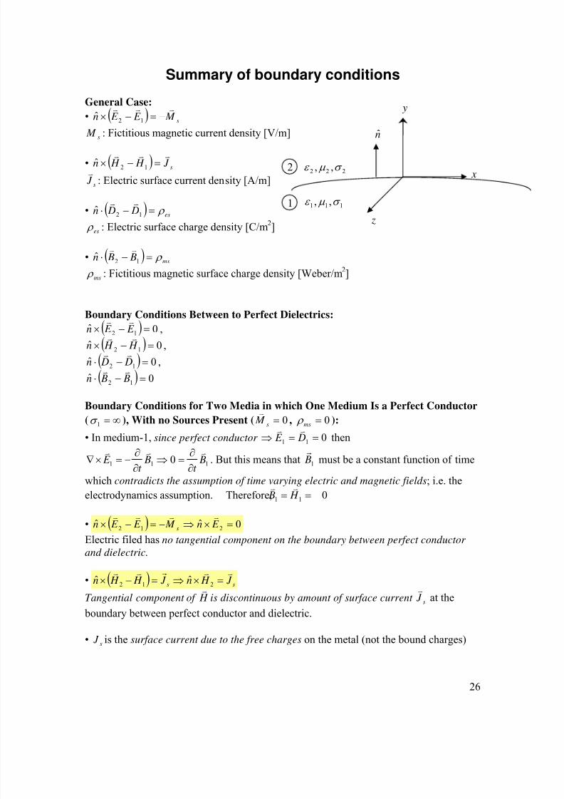
Summary of boundary conditions General Case:• ( ) sM E E n

vvv

−=−×12ˆ

sM : Fictitious magnetic current density [V/m] • ( ) sJ H H n

vvv

=−×12ˆ

sJ v

: Electric surface current density [A/m] • ( ) esDDn ρ =−⋅

12ˆvv

esρ : Electric surface charge density [C/m 2] • ( ) msBBn ρ =−⋅

12ˆvv

msρ : Fictitious magnetic surface charge density [Weber/m 2] Boundary Conditions Between to Perfect Dielectrics:

( ) 0ˆ 12=−× E E n

vv

,

( ) 0ˆ 12 =−× H H nvv

,

( ) 0ˆ 12 =−⋅ DDnvv

,

( ) 0ˆ 12=−⋅ BBn

vv

Boundary Conditions for Two Media in which One Medium Is a Perfect Conductor

( ∞=1σ ), With no Sources Present ( 0=sM v

, 0=msρ ):• In medium-1, since perfect conductor 011 ==⇒ DE

vv

then

111 0 Bt

Bt

E vvv

∂∂=⇒

∂∂−=×∇ . But this means that 1B

r

must be a constant function of time

which contradicts the assumption of time varying electric and magnetic fields ; i.e. theelectrodynamics assumption. Therefore, 011

== H Bvv

• ( ) 0ˆˆ 212

=×⇒−=−× E nM E E n s

vvvv

Electric filed has no tangential component on the boundary between perfect conductor and dielectric. • ( ) ss J H nJ H H n

vvrvv

=×⇒=−× 212 ˆˆ

Tangential component of H v

is discontinuous by amount of surface current sJ v

at theboundary between perfect conductor and dielectric. • sJ is the surface current due to the free charges on the metal (not the bound charges)



• ( ) eses DnDDn ρ ρ =⋅⇒=−⋅

212 ˆˆvvv

Electric field has only normal component on the boundary between perfect conductor anddielectric.

• ( ) 0ˆˆ 212 =⋅⇒=−⋅ BnBBn ms

vvv

ρ Magnetic field has no normal component on the boundary between perfect conductor and dielectric. Boundary Conditions Between TwoMedium one of which Is a PerfectMagnetic Material (the medium hasinfinite magnetic conductivity, i.e.

01

=t

H v

) and no sources are present

( 0=esρ , 0=sJ v

) • Here 00 11

=⇒= BH vv

, 011== DE

vv

• ( ) ss M E nM E E n

vvvvv

−=×⇒−=−×212 ˆˆ

Electric filed is tangential to the boundary • ( ) 0ˆˆ 212 =×⇒=−× H nJ H H n s

vvvv

Magnetic filed has no tangential component on the boundary

• ( ) 0ˆˆ 212

=⋅⇒=−⋅ DnDDn es

vvv

ρ Electric filed has no normal component at the boundary • ( ) msms BnBBn ρ ρ =⋅⇒=−⋅

212 ˆˆvvv

Magnetic field is normal to the boundary

metal

E vE

v

course notes set 1

Documents