12/28/2010 1

Module 22: Simple Harmonic Oscillation and Torque 22.1 Introduction We have already used Newton’s Second Law or Conservation of Energy to analyze systems like the bloc-spring system that oscillate. We shall now use torque and the rotational equation of motion to study oscillating systems like pendulums or torsional springs. 22.2 Simple Pendulum A pendulum consists of an object hanging from the end of a string or rigid rod pivoted about the point S . The object is pulled to one side and allowed to oscillate. If the object has negligible size and the string or rod is massless, then the pendulum is called a simple pendulum. The force diagram for the simple pendulum is shown in Figure 22.1.

Figure 22.1 A simple pendulum.

The string or rod exerts no torque about the pivot point S . The weight of the object has radial r̂ - and !̂ - components given by m

!g = mg(cos! r̂ " sin! !̂) (22.2.1) and the torque about the pivot point S is given by

!!S =

!rS , m " m!g = l r̂ " m g(cos# r̂ $ sin# #̂) = $l m g sin# k̂ (22.2.2) and so the component of the torque in the z -direction (into the page in Figure 22.1 for ! positive, out of the page for ! negative) is (! S )z = "mgl sin# . (22.2.3) The moment of inertia of a point mass about the pivot point S is

12/28/2010 2

2

SI ml= . (22.2.4) From the rotational dynamical equation is

(! S )z = IS" # IS

d 2$

dt2

%mgl sin$ = ml2 d 2$

dt2 . (22.2.5)

Thus we have the equation of motion for the simple pendulum,

2

2 sind gdt l!

!= " . (22.2.6)

When the angle of oscillation is small, then we can use the small angle approximation sin! !" ; (22.2.7) the rotational dynamical equation for the pendulum becomes

2

2

d gdt l!

!" # . (22.2.8)

This equation is similar to the object-spring simple harmonic oscillator differential equation from (add reference),

2

2

d x kx

dt m= ! , (22.2.9)

which describes the oscillation of a mass about the equilibrium point of a spring. Recall that in (add reference), the angular frequency of oscillation was given by

springkm

! = . (22.2.10)

By comparison, the frequency of oscillation for the pendulum is approximately

pendulumgl

! " , (22.2.11)

with period

12/28/2010 3

pendulum

2 2 lTg

!!

"= # . (22.2.12)

A procedure for determining the period for larger angles is given in Appendix 22.A. 22.3 Physical Pendulum A physical pendulum consists of a rigid body that undergoes fixed axis rotation about a fixed point S (Figure 22.2). The gravitational force acts at the center of mass of the physical pendulum. Suppose the center of mass is a distance cml from the pivot point S .

Figure 22.2 Physical pendulum. The analysis is nearly identical to the simple pendulum. The torque about the pivot point is given by

!!S =

!rS , cm " m!g = lcmr̂ " m g(cos# r̂ $ sin# #̂) = $lcmm g sin# k̂ . (22.3.1) Following the same steps that led from Equation (22.2.2) to Equation (22.2.6), the rotational dynamical equation for the physical pendulum is

( )

2

2

2

cm 2sin .

S S Sz

S

dI Idt

dmgl Idt

!" #

!!

= =

$ =

(22.3.2)

Thus we have the equation of motion for the physical pendulum,

12/28/2010 4

2

cm2 sin

S

d mgldt I!

!= " . (22.3.3)

As with the simple pendulum, for small angles sin! !" and Equation (22.3.3) reduces to the simple harmonic oscillator equation with angular frequency

cmpendulum

S

mg lI

! " (22.3.4)

and period

physicalpendulum cm

2 2 SITm g l

!!

"= # . (22.3.5)

It is sometimes convenient to express the moment of inertia about the pivot point in terms of cml and cmI using the parallel axis theorem (add link), with ,cm cmSd l! ,

2cm cmSI I ml= + , with the result

cm cmphysical

cm

2 l ITg m g l

!" + . (22.3.6)

Thus, if the object is “small” in the sense that 2

cm cmI ml! , the expressions for the physical pendulum reduce to those for the simple pendulum. Note that this is not the case shown in Figure 22.11. 22.3.1 Example: Oscillating rod A physical pendulum consists of a uniform rod of length d and mass m pivoted at one end. The pendulum is initially displaced to one side by a small angle !0 and released from rest. You can then approximate sin! " ! (with ! measured in radians). Find the period of the pendulum.

We shall find the period of the pendulum using two different methods.

1. Applying the torque equation about the pivot point.

12/28/2010 5

2. Applying the energy equation. Applying the torque equation about the pivot point. With our choice of rotational coordinate system the angular acceleration is given by

!! =

d 2"

dt2 k̂ . (22.3.7)

The force diagram on the pendulum is shown below. In particular, there is an unknown pivot force, the gravitational force acting at the center of mass of the rod.

The torque about the pivot point is given by

!!P =

!rP,cm " m!g . (22.3.8) The rod is uniform, therefore the center of mass is a distance d / 2 from the pivot point. The gravitational force acts at the center of mass, so the torque about the pivot point is given by

!!P = (d / 2)r̂ " mg(# sin$ $̂ + cos r̂) = #(d / 2)mg sin$ k̂ . (22.3.9)

The rotational dynamical equation (torque equation) is

!!P = IP

!" . (22.3.10)

Therefore

!(d / 2)mg sin" k̂ = IP

d 2"

dt2 k̂ . (22.3.11)

When the angle of oscillation is small, then we can use the small angle approximation

12/28/2010 6

sin! " ! . (22.3.12) Then the torque equation becomes

d 2!

dt2 +(d / 2)mg

IP

! = 0 (22.3.13)

which is the simple harmonic oscillator equation. The angular frequency of oscillation for the pendulum is approximately

!0 "

(d / 2)mgIP

. (22.3.14)

The moment of inertia of a rod about the end point P is IP = (1 / 3)md 2 therefore the angular frequency is

!0 "

(d / 2)mg(1 / 3)md 2 =

(3 / 2)gd

(22.3.15)

with period

T =

2!"0

# 2!23

dg

. (22.3.16)

Applying the energy equation. Take the zero point of gravitational potential energy to be the point where the center of mass of the pendulum is at its lowest point, that is, ! = 0 .

When the pendulum is at an angle ! the potential energy is

12/28/2010 7

( )1 cos2dU m g != " . (22.3.17)

The kinetic energy of rotation about the pivot point is

212rot pK I != . (22.3.18)

The mechanical energy is then

( ) 211 cos

2 2rot pd

E U K m g I! "= + = # + , (22.3.19)

with 2(1/ 3)PI md= . There are no non-conservative forces acting, so the mechanical energy is constant, and therefore its time derivative is zero

0 sinè2 p

dE d d dm g Idt dt dt

! ""= = + . (22.3.20)

Recall that /d dt! "= and 2 2/ /d dt d dt! "= so Eq. (22.3.20) becomes

2

20 sin2 pd dm g I

dt!

!" "= + . (22.3.21)

Therefore two solutions, 0! = , in which the same remains at the bottom of the swing and

2

20 sin2 pd dm g I

dt!

!= + (22.3.22)

Using the small angle approximation, we have the simple harmonic oscillator equation (Eq. (22.3.13))

2

2

( / 2) 0p

d m g ddt I!

!+ = . (22.3.23)

22.3.2 Example: Torsional Oscillator Solution A disk with moment of inertia about the center of mass cmI rotates in a horizontal plane. It is suspended by a thin, massless rod. If the disk is rotated away from its equilibrium position by an angle ! , the rod exerts a restoring torque given by cm! "#= $ . At 0t = ,

12/28/2010 8

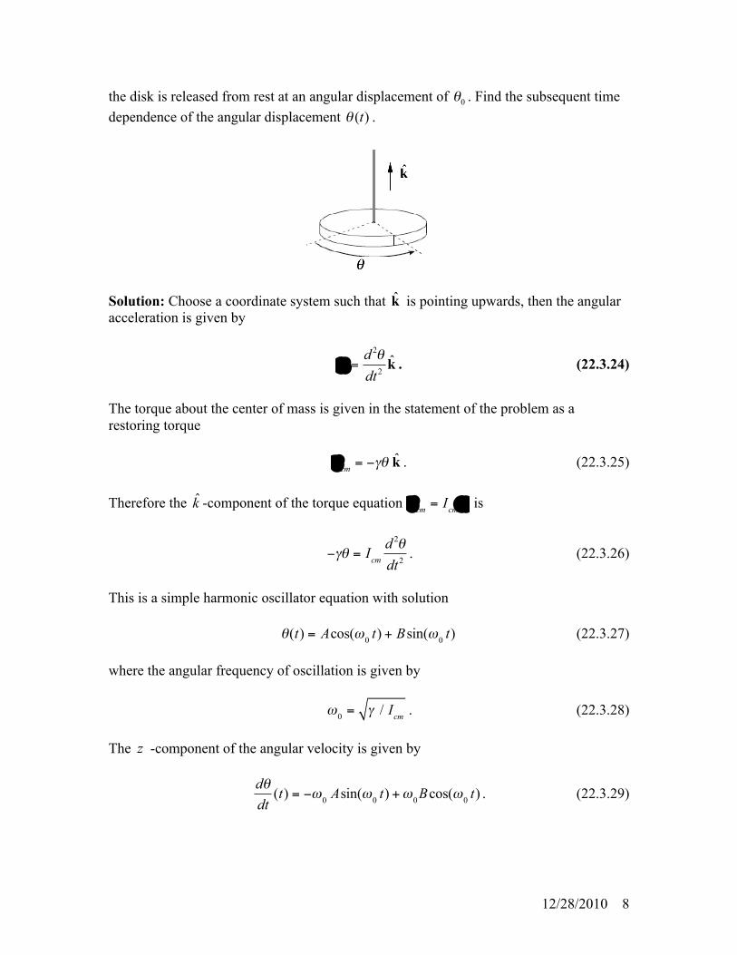
the disk is released from rest at an angular displacement of 0! . Find the subsequent time dependence of the angular displacement ( )t! .

Solution: Choose a coordinate system such that k̂ is pointing upwards, then the angular acceleration is given by

!! =

d 2"

dt2 k̂ . (22.3.24)

The torque about the center of mass is given in the statement of the problem as a restoring torque

!!cm = "#$ k̂ . (22.3.25)

Therefore the k̂ -component of the torque equation

!!cm = Icm

!" is

!"# = Icm

d 2#

dt2 . (22.3.26)

This is a simple harmonic oscillator equation with solution !(t) = Acos("0 t) + Bsin("0 t) (22.3.27) where the angular frequency of oscillation is given by !0 = " / Icm . (22.3.28) The z -component of the angular velocity is given by

d!dt

(t) = "#0 Asin(#0 t) +#0 Bcos(#0 t) . (22.3.29)

12/28/2010 9

The initial conditions at 0t = , are that 0( 0)t A! != = = , and (d! / dt)(t = 0) ="0 B = 0 . Therefore !(t) = !0 cos( " / Icm t) . (22.3.30)

Appendix 22.A: Higher-Order Corrections to the Period for Larger Amplitudes of a Simple Pendulum In Section 22.2 we found that using the small angle approximation the period for a simple pendulum is (22.2.12)

pendulum

2 2 lTg

!!

"= # .

How good is this approximation? If the pendulum is pulled out to an initial angle 0! that is not small (such that our first approximation sin! !" no longer holds) then our expression for the period is no longer valid. We then would like to calculate the first-order (or higher-order) correction to the period of the pendulum. Let’s first consider the mechanical energy, a conserved quantity in this system. Choose an initial state when the pendulum is released from rest at an angle 0! ; this need not be at time 0t = , and in fact later in this derivation we’ll see that it’s inconvenient to choose this position to be at 0t = . Choose for the final state the position and velocity of the bob at an arbitrary time t . Choose the zero point for the potential energy to be at the bottom of the bob’s swing (Figure 22.A.1).

Figure 22.A.1 Energy states for a simple pendulum. The initial mechanical energy is 0 0 0 0(1 cos )E K U mg l != + = " . (22.A.1) The tangential velocity of the bob at an arbitrary time t is given by

12/28/2010 10

tandv ldt!

= , (22.A.2)

and the kinetic energy at the final state is

2

2tan

1 12 2f

dK mv m ldt!" #= = $ %

& '. (22.A.3)

The final mechanical energy is then

21

(1 cos )2f f f

dE K U m l m g ldt!

!" #= + = + $% &' (

. (22.A.4)

Since the tension in the string is always perpendicular to the displacement of the bob, the tension does no work and mechanical energy is conserved, 0fE E= . Thus

12

m l d!dt

"

#$%

&'

2

+ m g l (1( cos!) = m g l (1( cos!0 )

l d!dt

"

#$%

&'

2

= 2gl

(cos! ( cos!0 ).

(22.A.5)

We can solve Equation (22.A.5) for the angular velocity as a function of ! ,

02

cos cosd gdt l!

! != " . (22.A.6)

Note that we have taken the positive square root, implying that / 0d dt! " . This clearly cannot always be the case, and we should change the sign of the square root every time the pendulum’s direction of motion changes. For our purposes, this is not an issue. If we wished to find an explicit form for either !(t) or ( )t ! , we would have to consider the signs in Equation (22.A.6) more carefully. Before proceeding, it’s worth considering the difference between Equation (22.A.6) and the equation for the simple pendulum in the simple harmonic oscillator limit,

2 2022 2

d gdt l! ! != " . (22.A.7)

In both Equations (22.A.6) and (22.A.7) the last term in the square root is proportional to the difference between the initial potential energy and the final potential energy. The

12/28/2010 11

final potential energy for the two cases is plotted in Figures 22.A.2 below for ! " !# < < on the left and / 2 / 2! " !# < < on the right (the vertical scale is in units of mgl ).

Figures 22.A.2 Potential energies as a function of displacement angle.

It would seem to be to our advantage to express the potential energy for an arbitrary displacement of the pendulum as the difference between two squares. This is done by recalling the trigonometric identity 1! cos" = 2sin2(" / 2) (22.A.8) with the result that Equation (22.A.6) may be re-expressed as

d!dt

=2gl

2(sin2(!0 / 2) " sin2(! / 2)) . (22.A.9)

(Note that using Equation (22.A.8) is “undoing” one step of (22.A.5).) Equation (22.A.9) is separable,

( ) ( )2 20

2sin / 2 sin / 2

d g dtl

!

! !=

" (22.A.10)

What comes next may seem like it’s been pulled out of a hat. The motivation is analogous to for the simple harmonic oscillator. That is, rewrite Equation (22.A.10) as

( ) ( )( )

2

0 20

2sin / 2

sin / 2 1sin / 2

d g dtl

!

!!

!

=

"

. (22.A.11)

12/28/2010 12

The ratio sin(! / 2) / sin(!0 / 2) in the square root in the denominator will oscillate (but not with simple harmonic motion) between 1! and 1, and so we will make the identification

sin! =

sin(" / 2)sin("0 / 2)

. (22.A.12)

If ! were proportional to the time t , the motion would be simple harmonic motion. We don’t expect this to be the case, but we might make some simplifications in doing the needed integration, and allow comparison to simple harmonic motion. Let 0sin( / 2)k != , so that

sin!2= k sin"

cos!2= 1# sin2 !

2$

%&'

()

1 2

= (1# k 2 sin2")1 2. (22.A.13)

Please be sure to note that here 0sin( / 2)k != is a dimensionless parameter of the system, not a spring constant. The integral in (22.A.11) can then be rewritten as

2

21 sind g dt

lk!

"=

#$ $ . (22.A.14)

From differentiating the first expression in Equation (22.A.13), we have that

2

2

2

2 2

1cos cos2 2

1 sincos2 2cos( / 2) 1 sin ( / 2)

1 sin2 .

1 sin

d k d

d k d k d

k dk

!! " "

""! " "

! !

""

"

=

#= =

#

#=

#

(22.A.15)

Substituting the last equation in (22.A.15) into the left-hand side of the integral in (22.A.14) yields

12/28/2010 13

2

2 2 2 2 2

1 sin2 21 sin 1 sin 1 sink dd

k k k! !

!! ! !

"=

" " "# # . (22.A.16)

Thus the integral in Equation (22.A.14) becomes

2 21 sind g dt

lk!

!=

"# # . (22.A.17)

This integral is one of a class of integrals known as elliptic integrals. We will encounter a similar integral when we solve the Kepler Problem, where the orbits of an object under the influence of an inverse square gravitational force are determined. We find a power series solution to this integral by expanding the function

(1! k 2 sin2")!1 2 = 1+

12

k 2 sin2" +38

k 4 sin4" + # # # . (22.A.18)

The integral in Equation (22.A.17) then becomes

2 2 4 41 31 sin sin2 8

gk k d dtl

! ! !" #+ + + $ $ $ =% &' () ) . (22.A.19)

Now let’s integrate over one period. Set 0t = when 0! = , the lowest point of the swing, so that sin 0! = and 0! = . One period T has elapsed the second time the bob returns to the lowest point, or when 2! "= . Putting in the limits of the ! -integral, we can integrate term by term, noting that

12

k 2 sin2! d!0

2"

# =12

k 2 12

(1$ cos(2!))0

2"

# d!

=12

k 2 12! $

sin(2!)2

%

&'(

)*0

2"

=12"k 2 =

12" sin2 +0

2.

(22.A.20)

Thus, from Equation (22.A.19) we have that

12/28/2010 14

2 2 2 4 4

0 0

2 0

1 31 sin sin2 8

12 sin2 2

T gk k d dtl

g Tl

!" " "

#! !

$ %+ + + & & & =' () *

+ + & & & =

+ +, (22.A.21)

We can now solve for the period,

2 012 1 sin4 2

lTg

!" # $= + + % % %& '

( ). (22.A.22)

If the initial angle is small compared to 1 (measured in radians), 0 1! << , then

2 20 0sin ( / 2) / 4! !" and the period is approximately

2 20 0 0

1 12 1 116 16

lT Tg

! " "# $ # $% + = +& ' & '( ) ( )

, (22.A.23)

where

0 2 lTg

!= (22.A.24)

is the period of the simple pendulum with the standard small angle approximation. The first order correction to the period of the pendulum is then

21 0 0

116

T T!" = . (22.A.25)

Figure 22.A.3 below shows the three functions given in Equation (22.A.24) (the horizontal, or red plot if seen in color), Equation (22.A.23) (the middle, parabolic or green plot) and the numerically-integrated function obtained by integrating the expression in Equation (22.A.17) (the upper, or blue plot) between 0! = and 2! "= as a function of k = sin(!0 / 2) . The plots demonstrate that Equation (22.A.24) is a valid approximation for small values of 0! , and that Equation (22.A.23) is a very good approximation for all but the largest amplitudes of oscillation. The vertical axis is in units of /l g . Note the displacement of the horizontal axis.

12/28/2010 15

Figure 22.A.3 Pendulum Period Approximations as Functions of Amplitude.

12/28/2010 16

MIT OpenCourseWare http://ocw.mit.edu 8.01SC Physics I: Classical Mechanics For information about citing these materials or our Terms of Use, visit: http://ocw.mit.edu/terms.