covariance analysis for deep-space satellites with radar and

Paper AAS 05-314

COVARIANCE ANALYSIS FOR DEEP-SPACE SATELLITES WITH RADAR AND

OPTICAL TRACKING DATA

James G. Miller

The MITRE Corporation

AAS/AIAA Astrodynamics Specialists Conference

AAS

Lake Tahoe, CA, August 7-11, 2005

Publications Office, P.O. Box 28130, San Diego, CA 92198

SBORG

Text Box

Approved for Public Release; Distribution Unlimited Case #05-0949

AAS 05-314

COVARIANCE ANALYSIS FOR DEEP-SPACE SATELLITES WITH RADAR AND OPTICAL TRACKING DATA

James G. Miller*

Covariance analysis for the special perturbations orbit determination problem for deep-space satellites is considered to determine the relative merit of radar and optical tracking data. Deep-space radars provide very accurate range measurements, but less accurate angle measurements. Optical sensors provide very accurate angle measurements, but make no range measurements since they are passive systems. The relationship of the size of the spatial part of the covariance to the relative track density of radar and optical tracks in the orbit determination fit interval is illustrated for various satellite orbits, including circular semi-synchronous, highly eccentric semi-synchronous, and geosynchronous.

INTRODUCTION The US Strategic Command Space Surveillance Network (SSN) is tasked to track satellites to maintain a special perturbations (SP) satellite catalog at the Space Control Center (SCC) at Cheyenne Mountain Air Force Station and at the Alternate Space Control Center (ASCC) at Dahlgren, VA. There is sufficient track capacity in the SSN to provide many tracks per day on near-earth satellites with period less than 225 minutes. However, there is not enough capacity in the SSN to track every deep-space satellite with period greater than or equal to 225 minutes at least once per day. The SSN has 11 ground-based optical sensors dedicated to tracking deep-space satellites, but such sensors are limited to night time viewing with clear weather. The Space Based Visible (SBV) sensor onboard the Midcourse Space Experiment (MSX) satellite is the only optical sensor that does not have either of these limitations. The recent upgrade of the Ground-based Electro-Optical Deep-Space Surveillance (GEODSS) sites with Charged-Coupled Devices (CCDs) has more than doubled the track capacity of the GEODSS sites. It is now feasible to obtain an optical track on each deep-space satellite every other day. The situation is much worse for obtaining radar tracks on deep-space satellites. There are only three deep-space radars in the SSN, namely ALTAIR at the Regan Test Site on the Kwajalein atoll, the Millstone Hill radar in Massachusetts, and the Globus II radar in Norway. The track capacity of each of these radars is very limited due to the necessity to integrate many pulses over an extended period of time in order to build up the signal-to-noise ratio to obtain a detection. Because a radar is an active system that transmits a radio frequency wave and receives the reflected wave from the satellite, the sensitivity of a radar is inversely proportional to the fourth power of the range to the satellite. These radars make very accurate range and range rate measurements, but less accurate angle measurements. Because an optical sensor is a passive system that receives reflected light from the sun, the sensitivity of an optical sensor is inversely proportional to the square of the range to the satellite. The ability of an optical sensor to detect a satellite also depends on the solar phase angle. Optical sensors provide very accurate angle measurements at fast integration times, but provide no range measurements.

* The MITRE Corporation, 1155 Academy Park Loop, Colorado Springs, CO 80910-3704, USA.

The new SP Sensor Tasking Prototype1 that tasks the SSN to maintain the SP satellite catalog has the ability to manage requirements for radar and optical tracks independently. Covariance analysis for the SP orbit determination problem for deep-space satellites is used to determine the relative merit of radar and optical tracking data. This analysis will be used to provide track requirements for the SP Sensor Tasking Prototype for deep-space satellites. COVARIANCE ANALYSIS The SP differential correction to a state vector is obtained by solving the linear equation 1. AX = B by weighted least squares, where the matrix A is obtained as the product of the partial derivatives of the measurements with respect to the state variables times the state transition matrix, the column vector X is the differential correction (DC) to the state vector, and the column vector B is the difference between the observed sensor measurements and the predicted measurements obtained by propagating the state vector to the time of the observations. The matrix D is the diagonal matrix whose entries are the reciprocals of the standard deviations of the sensor measurement errors. The weighted least squares problem is obtain by multiplying both sides of equation Eq. (1) by D, which yields 2. (DA)X = DB. The optimal least squares solution of Eq. (2) satisfies the normal equations 3. (ATWA)X = ATWB, where W = DTD and the superscript T indicates the transpose of the matrix. The covariance matrix C is the inverse of ATWA and is given by 4. C = (ATWA)-1. Covariance analysis assumes the only errors are sensor measurement errors characterized by their standard deviations, and no model errors. The Air Force Space Command (AFSPC) Astrodynamics Standards Look Angle Module (LAMOD) is used to generate perfect simulated observations in an Orbit Determination Interval (ODI) by propagating an SP state vector. The left-hand side of Eq. (3) does not depend on the actual value of the sensor measurements, but only on the time of the observations and the standard deviation of the measurements. The perfect simulated observations are used in the AFSPC Special Perturbations Differential Correction (SPDC) software to obtain a value for the covariance matrix C. The covariance matrix is then propagated forward from epoch an ODI length of time to see how the errors grow. The least squares covariance matrix tends to be an optimistic estimate of the actual state vector errors, but this analysis is more concerned with the relative merit of radar versus optical tacking data, and not the absolute errors from the SPDC process with real observations. For this analysis, radar tracks consist of six observations and optical tracks consist of eight observations, which is typical of what the deep-space SSN sensors provide. A GEODSS telescope at Socorro and the Millstone radar are used as the sensors for this analysis. The force model used is a 24 by 24 gravitational potential, and solar and lunar perturbations.

ANALYSIS RESULTS Since the amount of reflected sun light is dependent on the solar phase angle, optical sensors tend to collect observations around the minimum phase angle. However, it is better for the orbit determination problem to have the tracks distributed around the orbit rather than at one point of the orbit. Figure 1 shows the extreme case where an optical sensor provides a track each day at the minimum solar phase angle for an ODI of 21 days on a circular, semi-synchronous satellite, and there is no radar data. The components u, v, and w are the radial, in-track, and cross-track errors, respectively, obtained from the square root of the diagonal elements in the spatial part of the of the covariance matrix. The figure shows the propagated covariance over one ODI from epoch, not the covariance over the ODI itself, even though there is no evidence of error growth over time. The in-track errors are very large for this extreme situation, and they have the same period as the period of the satellite, namely 12 hours. Figure 2 shows the same satellite where the tracks from day to day have some variability around the minimum solar phase angle. The in-track error is still the largest error for optical only tracking data, but it is now much smaller. The cross-track error is the smallest error with optical only data. These figures illustrates the point that optical sensors should vary the tracks from day to day about the minimum solar phase angle, and not take all the tracks right at the minimum phase angle.

Circular, Semi-Synchronous Satellite

0

5

10

15

20

25

30

35

40

45

50

0 24 48 72 96 120 144 168 192 216 240 264 288 312 336 360 384 408 432 456 480 504 528

Hours Since Epoch

km

uvw

Figure 1 21-Day ODI, 21 Optical Tracks at Minimum Solar Phase Angle


0

0.5

1

1.5

2

2.5

3

3.5

0 24 48 72 96 120 144 168 192 216 240 264 288 312 336 360 384 408 432 456 480 504 528

Hours Since Epoch

km

uvw

Figure 2 21-Day ODI, 21 Optical Tracks

Figure 3 shows the same satellite with one radar track each day and no optical data. For radar only data, the largest error is the cross-track error, and the smallest is the radial error. Over all, radar

only data provides a more accurate state vector than optical only data.


0

0.1

0.2

0.3

0.4

0.5

0.6

0.7

0.8

0.9

1

0 24 48 72 96 120 144 168 192 216 240 264 288 312 336 360 384 408 432 456 480 504 528

Hours Since Epoch

km

uvw

Figure 3 21-Day ODI, 21 Radar Tracks

The best results are obtained with a combination of optical and radar data. However, it is unrealistic to get very much radar data on deep-space satellites. A realistic goal is to get an optical track every other day and as few as necessary radar tracks to complement the optical data and drive down the

in-track error. Figure 4 shows the same satellite with an optical track every other day and just two radar tracks. This combination of optical and radar tracks has less error than either the optical only data or radar only data.


0

0.1

0.2

0.3

0.4

0.5

0.6

0.7

0.8

0.9

1

0 24 48 72 96 120 144 168 192 216 240 264 288 312 336 360 384 408 432 456 480 504 528

Hours Since Epoch

km

uvw

Figure 4 21-Day ODI, 11 Optical Tracks, 2 Radar Tracks

Figure 5 shows the same satellite with an optical track every other day and just one radar track. A comparison of Figure 2 and Figure 5 shows the importance of getting just one radar track, but two radar tracks within the ODI is preferable.


0

0.1

0.2

0.3

0.4

0.5

0.6

0.7

0.8

0.9

1

0 24 48 72 96 120 144 168 192 216 240 264 288 312 336 360 384 408 432 456 480 504 528

Hours Since Epoch

km

uvw

Figure 5 21-Day ODI, 11 Optical Tracks, 1 Radar Track

Figure 6 shows a highly eccentric, semi-synchronous satellite with an optical track every day and no radar data. The ODI is also 21 days. Again, the in-track error is the largest and the cross-track error is the smallest for optical only tracking data.

Highly Eccentric, Semi-Synchronous Satellite

0

0.2

0.4

0.6

0.8

1

1.2

1.4

1.6

1.8

2

0 24 48 72 96 120 144 168 192 216 240 264 288 312 336 360 384 408 432 456 480 504 528

Hours Since Epoch

km

uvw


Figure 7 shows the same satellite with one radar track each day and no optical data. Now, the in-track error is the largest and the radial error is the smallest for radar only data.


0

0.1

0.2

0.3

0.4

0.5

0.6

0.7

0 24 48 72 96 120 144 168 192 216 240 264 288 312 336 360 384 408 432 456 480 504 528

Hours Since Epoch

km

uvw


Figure 8 shows the same satellite with an optical track every other day and just two radar tracks. This combination of optical and radar tracks has less error than either the optical only data or radar only data.


0

0.02

0.04

0.06

0.08

0.1

0.12

0.14

0.16

0 24 48 72 96 120 144 168 192 216 240 264 288 312 336 360 384 408 432 456 480 504 528

Hours Since Epoch

km

uvw




0

0.05

0.1

0.15

0.2

0.25

0 24 48 72 96 120 144 168 192 216 240 264 288 312 336 360 384 408 432 456 480 504 528

Hours Since Epoch

km

uvw


Figure 10 shows a geosynchronous satellite with an optical track every day and no radar data. The ODI is 28 days. Again, the in-track error is the largest and the cross-track error is the smallest for optical only tracking data.

Geosynchronous Satellite

0

1

2

3

4

5

6

7

8

0 24 48 72 96 120 144 168 192 216 240 264 288 312 336 360 384 408 432 456 480 504 528 552 576 600 624 648 672 696

Hours Since Epoch

km

uvw


Figure 11 shows the same satellite with one radar track each day and no optical data. Like the circular, semi-synchronous satellite, the cross-track error is the largest and the radial error is the smallest for radar only data on a geosynchronous satellite.


0

1

2

3

0 24 48 72 96 120 144 168 192 216 240 264 288 312 336 360 384 408 432 456 480 504 528 552 576 600 624 648 672 696

Hours Since Epoch

km

uvw


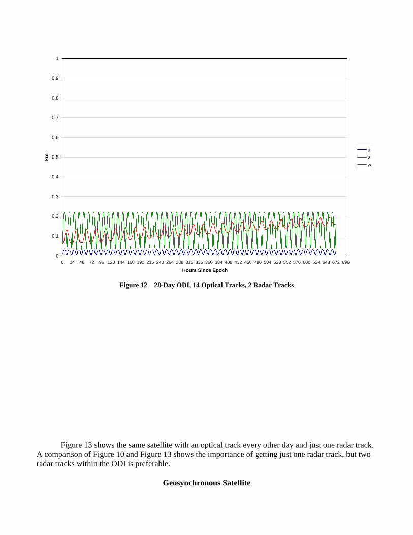
Figure 12 shows the same satellite with an optical track every other day and just two radar tracks. This combination of optical and radar tracks has less error than either the optical only data or radar only data.


0

0.1

0.2

0.3

0.4

0.5

0.6

0.7

0.8

0.9

1

0 24 48 72 96 120 144 168 192 216 240 264 288 312 336 360 384 408 432 456 480 504 528 552 576 600 624 648 672 696

Hours Since Epoch

km

uvw




0

0.1

0.2

0.3

0.4

0.5

0.6

0.7

0.8

0.9

1

1.1

1.2

0 24 48 72 96 120 144 168 192 216 240 264 288 312 336 360 384 408 432 456 480 504 528 552 576 600 624 648 672 696

Hours Since Epoch

km

uvw


CONCLUSIONS In general, radar only data provides a more accurate SP state vector than optical only data for deep-space satellites. However, the best case is a combination of optical and radar data, namely an optical track every other day and two radar tracks within the ODI. This covariance analysis will be used to establish separate optical and radar tracking requirements for deep-space satellites in the new SP Sensor Tasking Prototype, which will optimally allocate the very limited deep-space radar tracks. REFERENCES 1. James G. Miller, “A New Sensor Resource Allocation Algorithm for the Space Surveillance Network in Support of the

Special Perturbations Satellite Catalog,” AAS 03-669, AAS/AIAA Astrodynamics Specialist Conference, Big Sky, Montana, August 2003.

covariance analysis for deep-space satellites with radar and

Documents