covariant quantum mechanics and quantum...

Covariant quantum mechanicsand quantum symmetries

Josef Janyska1, Marco Modugno2, Dirk Saller3

1 Department of Mathematics, Masaryk University

Janackovo nam 2a, 662 95 Brno, Czech Republic

email: [email protected]

2 Department of Applied Mathematics, Florence University

Via S. Marta 3, 50139 Florence, Italy


3 Department of Mathematics, Mannheim University

A 5, Lehrstuhl I, 68131 Mannheim, Germany


Reprint of a paper published in“Recent Developments in General Relativity”,

Eds.: R. Cianci, R. Collina, M. Francaviglia, P. Fre,Genova, 2000. Springer, 2002, 179–201.

Reprinted with minor corrections on 2004.11.08.

Abstract

We sketch the basic ideas and results on the covariant formulation of quantummechanics on a curved spacetime with absolute time equipped with given gravita-tional and electromagnetic fields.

Moreover, we analyse the classical and quantum symmetries and show theirrelations.

Keywords: quantum mechanics, classical mechanics, general relativity, infinitesimal symmetries.

2000 MSC: 81P99, 81Q70, 81S10, 8399, 83E99, 53C05, 53D15, 53D50.

1

2 J. Janyska, M. Modugno, D. Saller

Contents

1 Introduction 2

2 Covariant quantum mechanics 52.1 Classical background . . . . . . . . . . . . . . . . . . . . . . . . . . . . . . 52.2 Covariant quantum mechanics . . . . . . . . . . . . . . . . . . . . . . . . . 12

3 Symmetries 173.1 Classical symmetries . . . . . . . . . . . . . . . . . . . . . . . . . . . . . . 183.2 Quantum symmetries . . . . . . . . . . . . . . . . . . . . . . . . . . . . . . 19

References 21

1 Introduction

Our fundamental picture of the physical world is due to the theory of general relativityand to the quantum field theory, which got great theoretical and experimental success.

The well established historical steps in classical theory have been: non relativistic the-ory, special relativity, general relativity. Analogously, the well established steps in quan-tum theory have been: non relativistic quantum mechanics, special relativistic quantumfield theory.

Unfortunately, these theories deal with different objects, use partially incompatiblemathematical methods and fulfill different requirements of covariance. In particular, thestandard formulation of quantum theories is highly based on concepts and methodsstrictly related to a flat spacetime and inertial observers, which conflict with generalcovariance on a curved spacetime.

So, a consistent formulation of quantum field theories and general relativity is a stillopen problem. The problem has at least two faces:

- general relativistic covariant formulation of quantum theories in a curved spacetime,- quantum theory of gravitational field.

The model of covariant quantum mechanics discussed in this paper is aimed at con-tributing to the first face of the problem, by means of new ideas and methods [23, 24, 25,4, 26, 27, 52, 31, 65, 66, 33, 67, 68, 29, 51, 55]. Namely, we study a general relativisticcovariant formulation of quantum mechanics on a classical background constituted by acurved spacetime fibred over absolute time and equipped with given spacelike Riemannianmetric, and gravitational and electromagnetic fields. Thus, we restrict our investigationjust to fundamental fields of classical and quantum mechanics, because we believe thatthis arena could possibly suggest us good ideas for unifying deeper fundamental theoriesof physics.

The framework of our model is allowed by the possible general relativistic formulationof classical physics in a curved spacetime with absolute time. This theory is well estab-

Genoa-2001-04-09.tex; [output 2011-08-19; 17:05]; p.2

Covariant quantum mechanics and quantum symmetries 3

lished in the literature [60, 61, 7, 8, 9, 10, 11, 12, 13, 19, 37, 38, 39, 40, 41, 42, 44, 45,47, 56, 62, 63], even if it is much less popular than the Einstein theory of relativity. Thistheory is rigorous and self–consistent from a mathematical viewpoint and describes thephenomena of classical physics by an approximation which is intermediate between theclassical theory and the Einstein theory of relativity.

The standard term “relativistic theory” links the special or general covariance withthe Minkowski or Lorentz metric. This usage is clearly motivated by the historical de-velopments of the Einstein theory. However, it would be more appropriate to refer theword “relativistic theory” only to its semantic meaning related to covariance. Indeed, thestandard usage would be highly misleading in our context. In fact, our model is generalrelativistic, in the sense of covariance, but it is not Minkowskian or Lorentzian.

Clearly, the Minkowski or Lorentz metric is physically related to the distinguishedconstant c. Actually, in our model this constant does not occur. The classical limit ofEinstein general relativity for c→∞ [13] is quite delicate, if we wish to understand thelimit of the geometric structures of the model and not only the limit of some measure-ments. In a sense, our model could be regarded as the “true” classical limit of Einsteingeneral relativity.

Our model can be regarded as an intermediate step between the standard non rela-tivistic quantum mechanics and a possible fully general relativistic quantum theory. Thisframework allows us to focus our attention on the general relativistic covariance andthe curved spacetime, detaching them from the difficulties due to the Lorentz metric.Actually, our choice seems to be quite fruitful.

The main new methods and achievements can be summarised as follows.First of all, our basic guide is the covariance (even more, the manifest covariance)

of the theory as heuristic requirement. Nowadays, the concept of “covariance” has beenformulated in a rigorous mathematical way through the geometric concept of “naturality”[35]. According to the covariance of the theory, time is not just a parameter, but a fun-damental object of the theory; moreover, the main objects of the theory are not assumedto be split into time and space components. As classical phase space we take the first jetspace of spacetime and not its tangent space; indeed, this minimal choice allows us to skipanholonomic constraints. Another consequence of our choices is that classical mechanicsis ruled not by a symplectic structure, but by a cosymplectic structure [46]; actually, wedo get a symplectic structure, but this describes only the spacelike aspects of classicaltheory and is insufficient to account for classical dynamics. An achievement of our theoryis the Lie algebra of “special quadratic functions” (different from the Poisson algebra),which allows us to treat energy, momentum and spacetime functions on the same footing.We emphasize the fact that classical mechanics can be formulated in a covariant way bya Lagrangian approach, but not by a Hamiltonian approach, because the Hamiltonianfunction depends essentially on an observer.

As far as quantum mechanics is concerned, all objects are derived, in a covariant way,from three minimal objects. Here, we have some novelties. The quantum bundle lives onspacetime and not on the phase space and the quantum connection is “universal”. Theseassumptions allow us to skip all problems of polarisations [70]. In a sense, we obtain



naturally a covariant polarisation and this is sufficient for our purposes. Indeed, we replacethe problematic search for such inclusions with a method of projectability , which turns outto be our implementation of covariance in the quantum theory. Another new assumptionconcerns the Hermitian metric of the quantum bundle, which takes its values in the spaceof spacelike volume forms. This assumption allows us to skip the problems related to half–densities. The Schroedinger equation is obtained, in a covariant way, through a Lagrangianapproach and not through the standard non covariant Hamiltonian approach. Indeed, weexhibit an explicit expression of the Schroedinger equation for any quantum system.The quantum operators arise automatically, in a covariant way, from the classificationof distinguished first and second order differential operators of the quantum frameworkand not from a quantisation requirement of a classical system [70]. The seat for thecovariant probabilistic interpretation of quantum mechanics is a Hilbert bundle, naturallyyielded by the quantum bundle, and not just a Hilbert space. Our theory provides explicitexpressions of all objects for any accelerated observer and yields, at the same time, aninterpretation in terms of gravitational field, according to the principle of equivalence.

In a few words, we start with really minimal geometric structures representing physicalfields and proceed along a thread naturally imposed by the only requirement of generalcovariance. We take the well established results of classical and quantum mechanics astouchstone of our model. On the other hand, according to the aims of our theory, wedisregard those standard methods for deriving quantum objects, which are incompatiblewith general covariance. Indeed, in the flat case, the results of our model reduce to theresults of the standard classical and quantum mechanics.

In this paper, we deal just with a given gravitational and electromagnetic field; thisis sufficient as classical background for our covariant model of quantum mechanics. Onthe other hand, our classical model can be completed by adding, in a covariant way, theequations linking the gravitational and electromagnetic fields to their mass and chargesources [25]. These equations are a covariant reduced version of the Einstein and Maxwellequations. In fact, due to the spacelike nature of the metric, there is no way to couplefully the gravitational and electromagnetic fields with the energy–momentum tensor andthe charge current, respectively. Just this is the main point which makes the Einsteinmodel physically much more complete than ours. On the other hand, in our quantummodel, the gravitational and electromagnetic fields are “external”, hence the relation ofthese fields with their sources does not play an effective role in this context.

The reader might be puzzled by the fact that we do not mention explicitly the rep-resentations of the (finite dimensional and infinite dimensional) groups involved in ourtheory. In fact, our natural geometric constructions provide these representations auto-matically. This is an outproduct of our manifestly covariant approach.

In our model we never make an essential use of the fact that the dimension of spacetimeis n = 1 + 3. We just need n ≥ 1 + 2. In fact we have applied our machinery to thequantisation of a rigid body, whose configuration space has dimension n = 1 + 3 + 3 [67].

Even more, in our model we never make an essential use of the fact that the spacelikemetric of spacetime is Riemannian; we just need that it is non degenerate on each fibre.So, we could, for instance, apply our machinery to a model of dimension 5, with a fibring



on an extra parameter, whose fibres are four dimensional Lorentzian manifolds. Sucha model would work pretty well mathematically, but we do not know any interestingphysical interpretation.

The scheme developed for covariant quantum mechanics of a scalar particle can beeasily and nicely extended to the case of a spin particle [4].

In spite of the differences of the starting scheme of spacetime, several steps of theabove methodology appeared to be usefully translable to the Einstein case. In particular,so far, we have been able to apply to the Einstein case the methods concerning theclassical phase space, the algebra of quantisable functions and the algebra of pre–quantumoperators [26, 30, 31, 28, 34, 32].

We hope that the new methods arising in our model could yield fruitful hints for apossible generally covariant formulation of quantum field theory in an Einstein framework.

Acknowledgements. This paper has been partially supported by Ministry of Ed-ucation of the Czech Republic under the Project MSM 143100009, Grant of the GA CRNo. 201/99/0296 (Czech Republic), Department of Applied Mathematics of Universityof Florence (Italy), Department of Mathematics of University of Mannheim (Germany),GNFM of INDAM (Italy), Project of cooperation N. 19/35 “Differential equation anddifferential geometry” between Czech Republic and Italy.

Marco Modugno would like to thank the organizers of the meeting for invitation andwarm hospitality.

2 Covariant quantum mechanics

2.1 Classical background

We start by sketching our covariant model of classical curved spacetime fibredover absolute time, and the related formulation of classical mechanics. We recallthe basic elements of the model and present new results, as well.

Classical spacetime. According to [25, 22], we postulate:(C.1) a classical spacetime E, which is an oriented four dimensional manifold;(C.2) the absolute time T , which is an oriented one dimensional affine space, associated

with the vector space T;(C.3) a time fibring t : E → T , which is a surjective map of rank 1;(C.4) a “scaled” spacelike metric g, which is a “scaled” Riemannian metric of the

fibres of spacetime;(C.5) a gravitational field K\, which is a linear connection of spacetime, which pre-

serves the time fibring and the spacelike metric and whose curvature fulfills the typicalsymmetry of Riemannian connections;

(C.6) a “scaled” electromagnetic field f , which is a “scaled” closed 2–form of spacetime.



Here, the word “scaled” used for the spacelike metric and the electromagnetic fieldmeans that these objects are tensorialised by a suitable scale factor which accounts forthe appropriate units of measurement.

A time unit of measurement will be denoted by u0 ∈ T and its dual by u0 ∈ T∗.We refer to charts of spacetime (xλ) = (x0, xi) adapted to the time fibring, to the

affine structure of time and to a time unit of measurement u0 ∈ T.

With reference to a given particle of mass m and charge q, in order to get rid ofany choice of length and mass units of measurement, it is convenient to “normalise” thespacelike metric and the electromagnetic field, by considering the Planck constant ~.

Thus, we consider the “re–scaled” spacelike metric G := m~ g, which takes its values in

T. Its coordinate expression is

G = G0ij u0 ⊗ di ⊗ dj ,

where di is the spacelike differential of the coordinate xi.Analogously, we consider the “re–scaled” electromagnetic field F := q

~ f , which is atrue form.

Accordingly, all objects derived from G and F will be re–scaled and will include themass and the charge of the particle, and the Planck constant as well.

As phase space for the classical particle we take the first order jet space J1E of thespacetime fibring [35]. We recall that J1E can be naturally identified with the affinesubspace of T∗⊗TE, whose elements v are normalised according to the condition v00 = 1(which is independent from the choice of a unit of measurement of time). The chartnaturally induced on the phase space by a spacetime chart is denoted by (x0, xi, xi0).

We have assumed a projection of spacetime over time, but, according to the principleof general relativity, not a distinguished splitting of spacetime into space and time. Inother words, for each spacetime vector X, we obtain, in a covariant way, its projectionon time X0 u0, but not a timelike and a spacelike component.

On the other hand, an observer is defined to be a section o : E → J1E. The coordinateexpression of an observer o is of the type o = u0 ⊗ (∂0 + oi0 ∂i). An observer o yields asplitting of each spacetime vector X into its observed timelike and spacelike componentsv = v0 (∂0 + oi0 ∂i) + (vi− v0 oi0) ∂i. A spacetime chart is said to be adapted to an observerif oi0 = 0. Conversely, each spacetime chart determines the observer, whose coordinateexpression is o = u0 ⊗ ∂0.

According to the principle of general relativity, we do not assume distinguished ob-servers.

The above objects C.1, ... , C.6 yield in a covariant way [25, 22]:- the scaled time form dt : E → T⊗ T ∗E of spacetime;- a spacelike volume form η and a spacetime volume form υ of spacetime;- a 2–form Ω\ : J1E → Λ2T ∗J1E of the phase space;



- a dt–vertical 2–vector Λ\ : J1E → Λ2V J1E of the phase space,- a second order connection γ\ : J1E → T∗ ⊗ TJ1E of spacetime,Here, we have used the symbol \ to label objects derived from the gravitational field.We obtain the following identities

i(γ\) dt = 1 , i(γ\) Ω\ = 0 , dt ∧ Ω\ ∧ Ω\ ∧ Ω\ 6≡ 0 ,

dΩ\ = 0 , L[γ\] Λ\ = 0 , [Λ\, Λ\] = 0 .

Hence, the pair (dt,Ω\) turns out to be a cosymplectic structure of the phase space[46].

Moreover, Λ\ and Ω\ yield inverse linear isomorphisms between the vector spaces ofdt–vertical vectors and γ\–horizontal forms of the phase space.

The Lie derivative of the spacelike metric G and of the spacelike volume form η withrespect to a vector field of E is well defined provided that the vector field is projectableon T .

If X is a vector field of E projectable on T , then we define its spacelike divergence bymeans of the equality divηX = L[X] η. We have the coordinate expression

divηX = X0 ∂0√|g|√|g|

+∂i(X

i√|g|)√

|g|.

It is convenient to add an electromagnetic term to the gravitational field, in a covariantway [25, 22], according to the formula

K = K\ +Ke :=K\ + 12

(dt⊗ F + F ⊗ dt) ,

i.e., in coordinates,

Khik = K\

hik , K0

ik = K\

0ik + 1

2Gij

0 Fjk , K0i0 = K\

0i0 +Gij

0 Fj0 ,

where F :=Gij0 Fjλ d

0 ⊗ ∂i ⊗ dλ.Then, the “total” object K turns out to be a connection of spacetime, which fulfills

the same properties postulated in (C.5). Moreover, all main formulas in classical andquantum mechanics concerning the given particle and involving the gravitational andelectromagnetic fields can be expressed through the “total” K and its derived objects,without the need of splitting it into its gravitational and electromagnetic components.

Proceeding with the total spacetime connection K as before, we obtain the “total”second order connection, 2–form and 2–vector

γ = γ\ + γe , Ω = Ω\ + Ωe , Λ = Λ\ + Λe ,

where the electromagnetic terms γe, Ωe and Λe turn out to be, respectively, the (re–scaled)Lorentz force, 1

2the (re–scaled) electromagnetic field and 1

2the (re–scaled) contravariant

spacelike electromagnetic field, i.e. the (re–scaled) magnetic field.



These total objects fulfill all properties fulfilled by the gravitational objects as above.

The total cosymplectic 2–form Ω encodes the full structure of spacetime (metric, gra-vitational field and electromagnetic field), hence it plays a central role in the theory.

We obtain the following coordinate expressions

γ0i0 = Kh

ik x

h0x

k0 + 2K0

ik x

k0 +K0

i0

Ω = G0ij

(di0 − γ0i0 d0 − (Kh

i0 +Kh

ik x

k0) (dh − xh0 d0)

)∧ (dj − xj0 d0)

Λ = Gij0

(∂i + (Ki

h0 +Ki

hk x

k0) ∂0h

)∧ ∂0j .

Classical mechanics. The classical mechanics can be achieved as follows.The second order connection γ yields, in a covariant way, the generalised Newton law

∇j1s = 0, for a motion s : T → E. Clearly, this equation splits into its gravitational andelectromagnetic components as ∇\j1s = γe j1s.

Moreover, the classical dynamics can be derived from Ω, by a Lagrangian formalism,in the following covariant way [52, 22, 36].

2.1 Proposition. The closed 2–form Ω admits locally horizontal potentials Θ :J1E → T ∗E, which are defined up to closed 1–forms of spacetime.

The horizontal potentials Θ have coordinate expression of the type

Θ = −(12G0ij x

i0 x

j0 − A0) d

0 + (G0ij x

j0 + Aj) d

i , with A ∈ Sec(E, T ∗E) .

A horizontal potential Θ and an observer o yield the classical potential A := o∗Θ :E → T ∗E, which is defined locally up to a closed form and depends on the observer.

2.2 Proposition. Let us consider a given horizontal potential Θ; if o and o = o + vare two observers, then the associated potentials A and A are related, in a chart adaptedto o, by the formula

A = A− 12G0ij v

i0 v

j0 d

0 +G0ij v

j0 d

i .

Therefore, each horizontal potential Θ determines a distinguished observer; in fact,there is a unique observer o, such that the spacelike component of the associated potentialA vanishes.

An observer o yields the observed 2–form Φ := 2 o∗Ω : E → Λ2T ∗E.

2.3 Proposition. We have Φλµ = ∂λAµ − ∂µAλ.We obtain also Φ0k := −G0

kjK0j0 and Φhk :=G0

hjKkj0 −G0

kjKhj0.

2.4 Proposition. A horizontal potential Θ yields, in a covariant way, the classicalLagrangian L : J1E → T ∗T , with coordinate expression

L = (12G0ij x

i0 x

j0 + Ai x

i0 + A0) d

0 ,



where Aλ are the components of the potential A observed by the observer o associatedwith the chart. The Lagrangian is defined locally and up to a gauge, but does not dependon any observer. The Poincare–Cartan form associated with the Lagrangian L turns outto be just Θ.

The Euler–Lagrange equation associated with L turns out to coincide with the gen-eralised Newton law.

2.5 Proposition. A horizontal potential Θ and an observer o yield the classicalHamiltonian H : J1E → T ∗T and the classical momentum P : J1E → T ∗E, defined asthe negative of the o–horizontal component and the o–vertical components of Θ, respec-tively. Thus, we can write

Θ = −H + P .

In an adapted chart, we have the coordinate expressions

H = (12G0ij x

i0 x

j0 − A0) d

0 , P = (G0ij x

j0 + Ai) d

i .

They are defined locally and up to a gauge, and depend on the choice of the observer.

The Newton law can be achieved also through H and P , by means of a Hamiltonianformalism; but this procedure is non covariant, as it depends on the choice of an observer.

Classical Lie algebras. Additionally, our structures yield further results on Liealgebras of functions and lifts of functions.

First of all, we obtain the Poisson Lie bracket f, g := Λ](df ∧ dg) for the functionsof phase space.

A function f of phase space is conserved along the solutions of the Newton law if andonly if γ.f = 0. We denote the space of conserved functions by Con(J1E, IR). This spaceturns out to be a subalgebra of the Poisson algebra.

The time fibring and the spacelike metric yield, in a covariant way, a distinguishedsubset of the set of functions of phase space [25]. Namely, we define a special quadraticfunction to be a function of phase space, whose second fibre derivative (with respect tothe affine fibres of phase space over spacetime) is proportional to the spacelike metric. Inother words, in coordinates, the special quadratic functions are the functions of the type

f = 12f 0G0

ij xi0 x

j0 + f iG0

ij xj0 +

o

f , with f 0, f i,o

f ∈ Map(E, IR) .

The time component of a special quadratic function f as above is defined to be the(coordinate independent) map f ′′ := f 0 u0 : E → T.

2.6 Proposition. The space of special quadratic functions Spec(J1E, IR) turns outto be a Lie algebra through the special Lie bracket

[[ f, g ]] := f, g+ γ(f ′′).g − γ(g′′).f ,



with coordinate expression

[[ f, g ]] 0 = f 0∂0g0 − g0∂0f 0 − fh∂hg0 + gh∂hf

0

[[ f, g ]] i = f 0∂0gi − g0∂0f i − fh∂hgi + gh∂hf

i

o

[[ f, g ]] = f 0∂0og − g0∂0

o

f − fh∂hog + gh∂h

o

f − (f 0 gk − g0 fk) Φ0k + fhgk Φhk .

2.7 Corollary. We have the following distinguished subalgebras of the special Liealgebra:

- the subalgebra Quan(J1E, IR) ⊂ Spec(J1E, IR) of quantisable functions f , whosetime components f ′′ depend only on time;

- the subalgebra Time(J1E, IR) ⊂ Quan(J1E, IR) of time functions f , whose timecomponents f ′′ are constant;

- the subalgebra Aff(J1E, IR) ⊂ Time(J1E, IR) of affine functions f , whose timecomponents f ′′ vanish;

- the subalgebra Map(E, IR) ⊂ Aff(J1E, IR) of spacetime functions .

2.8 Example. We obtain

L0,H0 ∈ Time(J1E, IR) , Pi ∈ Aff(J1E, IR) , xλ ∈ Map(E, IR) .

Clearly, the special bracket and the Poisson bracket coincide on Aff(J1E, IR).

We have distinguished lifts of special quadratic functions to vector fields of spacetimeand of phase space. Let us denote by Pro(E, TE) ⊂ Sec(E, TE) the subalgebra of vectorfields of E which are projectable on T .

2.9 Proposition. The time fibring and the spacelike metric yield, in a covariant way,for each f ∈ Spec(J1E, IR), the tangent lift X[f ] : E → TE, whose coordinate expressionis

X[f ] = f 0 ∂0 − f i ∂i .

The lift Spec(J1E, IR) → Sec(E, TE) : f 7→ X[f ] turns out to be a Lie algebramorphism (with respect to the special bracket and the standard Lie bracket, respectively);its kernel is Map(E, IR).


X[L0] = ∂0 − Ai0 ∂i , X[H0] = ∂0 , X[Pi] = −∂i , X[xλ] = 0 ,

where Ai0 :=Gij0 Aj.

We observe that X[L] :=u0⊗X[L0] turns out to be the unique observer for which thespacelike component of the observed potential A vanishes.

Moreover, X[H] :=u0 ⊗ X[H0] turns out to be just the observer by which we havedefined the Hamiltonian.



2.11 Proposition. For each vector field X of E projectable on T , the spacetimefibring yields, in a covariant way [35], the holonomic prolongation

X↑hol :=X(1) : J1E → TJ1E ,

whose coordinate expression is

X↑hol = Xλ ∂λ + (∂0Xi + ∂jX

i xj0 − ∂0X0 xi0) ∂0i .

This prolongation turns out to be an injective Lie algebra morphism.

2.12 Corollary. For each f ∈ Quan(J1E, IR), the time fibring yields, in a covariantway, the holonomic lift

X↑hol[f ] :=(X[f ]

)(1)

: J1E → TJ1E ,


X↑hol[f ] = f 0 ∂0 − f i ∂i − (∂0fi + ∂jf

i xj0 + ∂0f0 xi0) ∂

0i .

The lift Quan(J1E, IR) → Sec(J1E, TJ1E) : f 7→ X↑hol[f ] turns out to be a Liealgebra morphism (with respect to the special bracket and the standard Lie bracket,respectively); its kernel is Map(E, IR).


X↑hol[L0] = ∂0 − Ai0 ∂i − (∂0Ai0 + ∂jA

i0 x

j0) ∂

0i ,

X↑hol[H0] = ∂0 , X↑hol[Pi] = −∂i , X↑hol[xλ] = 0 .

For each function f of phase space, we obtain, in a covariant way, the dt–verticalHamiltonian lift Λ](df) : J1E → V J1E.

More generally, for each function f of phase space and for each time scale τ : J1E → T,we obtain the τ–Hamiltonian lift γ(τ) + Λ](df) : J1E → TJ1E.

In particular, we obtain the following result.

2.14 Proposition. For each f ∈ Spec(J1E, IR), the cosymplectic structure yields,in a covariant way, the Hamiltonian lift

X↑Ham[f ] := γ(f ′′) + Λ](df) : J1E → TJ1E ,


X↑Ham[f ] = f 0 ∂0 − f i ∂i +X i0 ∂

0i ,



where

X i0 = Gij

0

(12∂jf

0G0hkx

h0x

k0 + (−f 0∂0G

0jh + fk ∂kG

0jh +G0

hk ∂jfk)xh0

+ ∂jo

f + Φhjfh + f 0Φj0

).

The lift Quan(J1E, IR) → Sec(J1E, TJ1E) : f 7→ X↑Ham[f ] turns out to be a Liealgebra morphism (with respect to the special bracket and the standard Lie bracket,respectively); its kernel is Map(T , IR).


X↑Ham[H0] = ∂0 −Gij0 ∂0Pj ∂0i ,

X↑Ham[Pi] = −∂i +Ghj0 ∂iPh ∂0j , X↑Ham[x0] = 0 , X↑Ham[xi] = Gij

0 ∂0j .

The interest of the above Hamiltonian lift is due to the following result concerningthe projectability, which will play an important role in quantum mechanics.

2.16 Proposition. [25] The τ -Hamiltonian lift of a function f of phase space isprojectable on a vector field of spacetime if and only if f ∈ Spec(J1E, IR) and τ = f ′′.

Moreover, if these conditions are fulfilled, then the τ -Hamiltonian lift projects on thetangent lift of f .

2.2 Covariant quantum mechanics

We proceed by sketching our covariant model of quantum mechanics on a curvedspacetime fibred over absolute time. We recall the basic elements of the model andpresent new results, as well.

Quantum structure. According to [25, 22], for quantum mechanics of a chargedspinless particle in the above classical background (including the given gravitational andelectromagnetic external fields), we postulate:

(Q.1) a quantum bundle Q → E, which is a one dimensional complex vector bundleover spacetime;

(Q.2) a Hermitian metric h : E → C⊗(Q∗⊗EQ∗)⊗E Λ3V ∗E of the quantum bundle,with values in the complexified space of spacelike volume forms of spacetime.

Locally, we shall refer to a scaled complex quantum basis (b) normalised by the condi-tion h(b,b) = η. The associated scaled complex chart is denoted by (z). Then, we obtainthe scaled real basis (b1 ,b2) := (b, ib) and the associated scaled real chart (w1, w2).

If Ψ ∈ Sec(E, Q), then we write Ψ = Ψ1 b1 + Ψ2 b2 = ψ b, where Ψ1,Ψ2 and ψ are,respectively, the scaled real and complex components of Ψ.

Moreover, we consider the extended quantum bundle, Q↑ → J1E, obtained by ex-tending the base space of the quantum bundle to the classical phase space, which here



plays the role of space of classical observers.

Each system of connections o

Q of the quantum bundle parametrised by the classicalobservers induces, in a covariant way, a connection Q of the extended quantum bundle,which is said to be universal [17, 22]. The universal connections are characterised incoordinates by the condition Q0

i = 0.

Then, we postulate:(Q.3) a quantum connection Q of the extended quantum bundle, which is Hermitian,

universal and whose curvature is R[Q] = iΩ ⊗ I, where I = (w1 ∂w1 + w2 ∂w2) denotesthe identity vertical vector field of the quantum bundle.

We recall that Ω incorporates the mass m of the particle and the Planck constant ~.

2.17 Proposition. The coordinate expression of the quantum connection, with re-spect to a quantum basis and a spacetime chart, turns out to be locally of the type

Q0 = −iH0 , Qi = iPi , Q0i = 0 .

The above classical Hamiltonian H and momentum P are referred to the observer oassociated with the spacetime chart (xλ) and to a classical horizontal potential Θ of Ω,which is locally determined by the quantum connection Q and the quantum basis b.

Then, the gauge of the classical potential A := o∗Θ is determined by the quantum con-nection and the quantum basis. Moreover, we recall that A includes both the gravitationaland the electromagnetic potential.

These minimal geometric objects Q.1, ... , Q.3 constitute the only source, in a covariantway, of all further objects of quantum mechanics.

Actually, the quantum connection lives on the extended quantum bundle, whose basespace is the phase space; on the other hand, the covariance of the theory requires that thesignificant physical objects be independent from observers. This fact suggests a method ofprojectability, in order to get rid of the observers encoded in the phase space. Actually, wehave already used this method in the classical theory, just in view of these developmentsof quantum mechanics. Indeed, this method turns out to be fruitful.

Quantum dynamics. The quantum dynamics can be obtained in the following way.The method of projectability yields, in a covariant way, a distinguished quantum

Lagrangian (hence, the generalised Schroedinger equation, the quantum momentum andthe probability current) [25, 22].

Even more, the covariance implies the essential uniqueness of the above Lagrangianand of the Schroedinger equation [27, 29].

2.18 Proposition. The coordinate expression of the quantum Lagrangian is

L[Ψ] = 12

(i (ψ ∂0ψ − ψ ∂0ψ) + 2A0 ψ ψ

−Gij0 (∂iψ ∂jψ + AiAj ψ ψ)− iGij

0 Aj (ψ ∂iψ − ψ ∂iψ) + k ρ0 ψ ψ)



√|g| d0 ∧ d1 ∧ d2 ∧ d3 ,

where ρ is the scalar curvature of the fibres of spacetime determined by the spacelikemetric and k ∈ IR is a real constant (which is not determined by the covariance).

2.19 Corollary. The coordinate expression of the generalised Schroedinger equationturns out to be (

∂0 − iA0 + 12

∂0√|g|√|g|− 1

2i (

o

∆0 + k ρ0))ψ = 0 ,

whereo

∆0 :=Ghk0 (∂h − iAh) (∂k − iAk) +

∂h(Ghk0

√|g|)√

|g|(∂k − iAk)

is the spacelike quantum Laplacian.

2.20 Corollary. We obtain the conserved probability current with coordinate expres-sion

Ψ∗j = (ψ ψ) υ00 −Ghk0

(i 12

(ψ ∂hψ − ψ ∂hψ) + Ah ψ ψ)υ0k ,

where υ0λ := i(∂λ)√|g| d0 ∧ d1 ∧ d2 ∧ d3 .

Quantum operators. We obtain distinguished operators acting on the sections ofthe quantum bundle in the following covariant way.

First of all, we have a distinguished family of second order pre–quantum operators .

2.21 Proposition. The Schroedinger operator yields, for each time scale τ : E → T,the second order linear operator S(τ) : J2Q → Q, which acts on the sections Ψ of thequantum bundle, according to the coordinate expression

S(τ)[Ψ] = i τ 0(∂0 − iA0 + 1

2

∂0√|g|√|g|− 1

2i (

o

∆0 + k ρ0))ψ b .

In particular, each f ∈ Spec(J1E, IR) yields, in a covariant way, the second orderpre–quantum operator S[f ] :=S(f ′′).

Then, we obtain a distinguished family of first order operators, by classifying thevector fields of the quantum bundle which preserve the Hermitian metric.

A vector field Y of Q is said to be Hermitian if it is projectable on E and on T , isreal linear over its projection on E, and fulfills L[Y ]h = 0.

We denote the space of Hermitian vector fields of Q by Her(Q, TQ).

2.22 Proposition. A vector field Y of Q is Hermitian if and only if its coordinateexpression is of the type

Y ≡ Y [f ] = f 0 ∂0 − f i ∂i +(i (

o

f + A0 f0 − Ai f i)− 1

2divηX[f ]

)I ,



where f ∈ Quan(J1E, IR). The above expression of Y [f ] turns out to be independent ofthe choice of coordinates.

The space of Hermitian vector fields Her(E, TQ) is closed with respect to the Liebracket. Moreover, the map

Quan(J1E, IR)→ Her(Q, TQ) : f 7→ Y [f ]

is an isomorphism of Lie algebras (with respect to the special bracket and the standardLie bracket, respectively).

Furthermore, the map Her(Q, TQ) → Pro(E, TE) : Y [f ] 7→ X[f ] turns out to be acentral extension of Lie algebras by Map(E, i IR)⊗ I.

For each f ∈ Quan(J1E, IR), the vector field Y [f ] : Q → TQ is said to be thequantum lift of f .


Y [L0] = ∂0 − Ai0 ∂i −(iAiA

i0 + 1

2(∂0√|g|√|g|−∂i(A

i0

√|g|)√

|g|))I ,

Y [H0] = ∂0 − 12

∂0√|g|√|g|

I , Y [Pi] = −∂i + 12

∂i√|g|√|g|

I , Y [xλ] = ixλ I .

2.24 Corollary. Each quantisable function f yields, in a covariant way, the first orderoperator acting on the sections of the quantum bundle

Z[f ] := iL[Y [f ]

],

whose coordinate expression is, for each Ψ ∈ Sec(E, Q),

Z[f ].Ψ = i(f 0 ∂0ψ − f i ∂iψ −

(i (

o

f + A0 f0 − Ai f i)− 1

2divηX[f ]

)ψ)b .

For each quantisable function f , we say Z[f ] to be the associated first order pre–quantum operator . We denote the space of the first order pre–quantum operators byOper1(Q).

2.25 Proposition. The space Oper1(Q) turns out to be a Lie algebra through thebracket [

Z[f ], Z[g]]

:= − i(Z[f ] Z[g]− Z[g] Z[f ]

).

Moreover, the map Quan(J1E, IR) → Oper1(Q) : f 7→ Z[f ] turns out to be anisomorphism of Lie algebras (with respect to the special bracket and the above Lie bracket,respectively).




Z[H0].Ψ = i(∂0ψ + 1

2

∂0√|g|√|g|

ψ)b

Z[Pi].Ψ = −i(∂iψ + 1

2

∂i√|g|√|g|

ψ)b

Z[xλ].Ψ = xλ ψ b .

The above results appear to be a covariant “correspondence principle” yielding pre–quantum operators associated with quantisable functions.

However, we still need to introduce the Hilbert stuff carrying the standard probabilisticinterpretation of quantum mechanics. It can be done in the following covariant way [25,22].

Let us restrict our postulate C.3, by requiring that the fibring of spacetime over timemakes spacetime a bundle. Thus, we postulate that the fibres of spacetime are each otherisomorphic.

Then, we consider the infinite dimensional functional quantum bundle Hc → T , whosefibres are constituted by the compact support smooth sections, at fixed time, of thequantum bundle (“regular sections”). The Hermitian metric h equips this bundle witha pre–Hilbert metric 〈 , 〉. Then, a true Hilbert bundle H → T can be obtained by acompletion procedure. This bundle has no distinguished splittings into time and typeHilbert fibre; such a splitting can be obtained by choosing a classical observer.

Each regular section Ψ of the quantum bundle can be regarded as a section Ψ of thefunctional quantum bundle. Accordingly, each “regular” operator O acting on sectionsof the quantum bundle can be regarded as an operator O acting on the sections of thefunctional quantum bundle.

Our previous results yield, for each quantisable function f , two distinguished operators

acting on the sections of the functional quantum bundle, namely Z[f ] and S[f ]. Actually,in general, both operators do not act on the fibres of the functional bundle (at fixed time),because they involve the partial derivative ∂0.

On the other hand, we have the following results [25, 22, 51].

2.27 Proposition. Let f ∈ Quan(J1E, IR). Then, the combination

f := Z[f ]− S[f ]

acts on the fibres of the functional bundle. We have the following coordinate expression

f(Ψ) =(− 1

2f 0 (

o

∆0 + k ρ0)− i f j (∂j − iAj) +o

f − i 12

∂j(fj√|g|)√

|g|)ψ b .

Moreover, f is symmetric with respect to the Hermitian metric 〈 , 〉.



For the self–adjointness of f further global conditions on f are needed.

For each f ∈ Quan(J1E, IR), we say f to be the quantum operator associated with f .

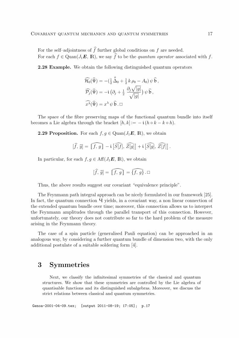
2.28 Example. We obtain the following distinguished quantum operators

H0(Ψ) = −(12

o

∆0 + 12k ρ0 − A0)ψ b ,

Pj(Ψ) = −i(∂j + 1

2

∂j√|g|√|g|

)ψ b ,

xλ(Ψ) = xλ ψ b .

The space of the fibre preserving maps of the functional quantum bundle into itselfbecomes a Lie algebra through the bracket [h, k] := − i (h k − k h).

2.29 Proposition. For each f, g ∈ Quan(J1E, IR), we obtain

[f , g] = [[ f, g ]] − i[S[f ], Z[g]

]+ i[S[g], Z[f ]

].

In particular, for each f, g ∈ Aff(J1E, IR), we obtain

[f , g] = [[ f, g ]] = f, g .

Thus, the above results suggest our covariant “equivalence principle”.

The Feynmann path integral approach can be nicely formulated in our framework [25].In fact, the quantum connection Q yields, in a covariant way, a non linear connection ofthe extended quantum bundle over time; moreover, this connection allows us to interpretthe Feynmann amplitudes through the parallel transport of this connection. However,unfortunately, our theory does not contribute so far to the hard problem of the measurearising in the Feynmann theory.

The case of a spin particle (generalised Pauli equation) can be approached in ananalogous way, by considering a further quantum bundle of dimension two, with the onlyadditional postulate of a suitable soldering form [4].

3 Symmetries

Next, we classify the infinitesimal symmetries of the classical and quantumstructures. We show that these symmetries are controlled by the Lie algebra ofquantisable functions and its distinguished subalgebras. Moreover, we discuss thestrict relations between classical and quantum symmetries.



3.1 Classical symmetries

We start by discussing the main results concerning symmetries of the classicalstructure.

Subalgebras. First we analyse further distinguished subalgebras of the Lie algebraof quantisable functions.

3.1 Proposition. We have the following distinguished subalgebras of the algebra ofquantisable functions:

– the subalgebra Hol(J1E, IR) ⊂ Quan(J1E, IR), which is constituted by the functionsf such that X↑hol[f ] = X↑Ham[f ];

– the subalgebra Unim(J1E, IR) ⊂ Quan(J1E, IR), which is constituted by the func-tions f such that divηX[f ] = 0;

– the subalgebra Self(J1E, IR) ⊂ Quan(J1E, IR), which is constituted by the func-tions f such that i(X↑hol[f ]) Ω = df .

If f ∈ Hol(J1E, IR), then we set

X↑[f ] :=X↑Ham[f ] = X↑hol[f ] .

3.2 Proposition. We have

Time(J1E, IR) ∩ Con(J1E, IR) = Time(J1E, IR) ∩ Self(J1E, IR) .

Then, we set

Clas(J1E, IR) := Time(J1E, IR) ∩ Con(J1E, IR)

= Time(J1E, IR) ∩ Self(J1E, IR)

and denote the space of the tangent lifts of elements of Clas(J1E, IR) by

Clas(E, TE) ⊂ Pro(E, TE) .

3.3 Proposition. We have

Time(J1E, IR) ∩ Con(J1E, IR) ⊂ Hol(J1E, IR)

Time(J1E, IR) ∩ Con(J1E, IR) ⊂ Unim(J1E, IR) .

3.4 Proposition. The special and the Poisson brackets coincide in Clas(J1E, IR).Hence, this space turns out to be a subalgebra of the Poisson and of the special algebras.

Moreover, Clas(E, TE) turns out to be closed with respect to the standard Liebracket.

We call the elements of Clas(J1E, IR) classical generators . This name will be justifiedby Proposition 3.5, Corollary 3.6 and Corollary 3.7.



Symmetries. A vector field X↑ ∈ Sec(J1E, TJ1E) is said to be a symmetry of theclassical structure if it is projectable on E and T and fulfills

L[X↑] dt = 0 , L[X↑] Ω = 0 .

We denote the space of symmetries of the classical structure by Clas(J1E, TJ1E).

3.5 Proposition. [55] A vector field X↑ of J1E projectable on E fulfills L[X↑] dt = 0and L[X↑] Ω = 0 if and only if, locally,

X↑ = X↑[f ] , with f ∈ Clas(J1E, IR) ,

where f is defined up to a constant.

3.6 Corollary. If f ∈ Clas(J1E, IR), then we obtain

L[X[f ]

]G = 0 , L

[X[f ]

]η = 0 , L

[X↑[f ]

]γ = 0 , L

[X↑[f ]

]K = 0 .

3.7 Corollary. If X is a vector field of E projectable on T , such that L[X↑hol]L = 0,then we obtain locally

X = X[f ] , X↑hol = X↑[f ] , with f ∈ Clas(J1E, IR) ,

where f is defined up to a constant.

3.2 Quantum symmetries

Eventually, we classify the vector fields of the extended quantum bundle whichpreserve the full quantum structure: all fibrings (on quantum bundle, on phasespace, on spacetime, on time), the Hermitian metric, the quantum connection. More-over, we compare the symmetries of the quantum structure with the symmetries ofthe quantum Lagrangian.

Symmetries of the quantum structure. A vector field Y ↑ of Q↑ is said to be asymmetry of the quantum structure if it is projectable on Q, J1E, E, T , is real linearover J1E and fulfills

L[Y ↑] dt = 0 , L[Y ↑]h = 0 , L[Y ↑]Q = 0 .

We denote the space of symmetries of the quantum structure by Quan(Q↑, TQ↑).

For each f ∈ Hol(J1E, IR), we define its extended quantum lift to be the vector fieldof the extended quantum bundle

Y ↑[f ] :=Q(X↑[f ]

)+(i f − 1

2divηX[f ]

)I .



3.8 Proposition. A vector field Y ↑ of Q↑ is a symmetry of the quantum structure ifand only if it is of the type

Y ↑ = Y ↑[f ] , with f ∈ Clas(J1E, IR) .

The space Quan(Q↑, TQ↑) is closed with respect to the Lie bracket. Moreover, themap Clas(J1E, IR) → Quan(Q↑, TQ↑) : f 7→ Y ↑[f ] is an isomorphism of Lie algebras(with respect to the special bracket and the standard Lie bracket, respectively).

Furthermore, the map Quan(Q↑, TQ↑)→ Clas(E, TE) : Y ↑[f ] 7→ X[f ] turns out tobe a central extension of Lie algebras by i IR⊗ I.

Symmetries of the quantum dynamics. Next, we compare the symmetries ofthe quantum connection and the symmetries of the quantum Lagrangian.

3.9 Proposition. For each f ∈ Quan(J1E, IR), we obtain, in a covariant way, theholonomic quantum lift of f , defined as the holonomic prolongation [35]

Yhol[f ] :=(Y [f ]

)(1)

: J1Q→ TJ1Q

of the quantum lift Y [f ], whose coordinate expression is

Yhol[f ] = f 0 ∂0 − f i ∂i− 1

2divηX[f ] (w1 ∂1 + w2 ∂2 − w1

λ ∂λ1 − w2

λ ∂λ2 )− 1

2∂λ divηX[f ] (w1 ∂λ1 + w2 ∂λ2 )

+ (f 0A0 − f iAi +o

f) (w1 ∂2 − w2 ∂1 + w1λ ∂

λ2 − w2

λ ∂λ1 )

+ ∂λ(f0A0 − f iAi +

o

f) (w1 ∂λ2 − w2 ∂λ1 )

− ∂0f 0 (w10 ∂

01 + w2

0 ∂02) + ∂λf

i (w1i ∂

λ1 + w2

i ∂λ2 ) .

3.10 Proposition. Let f ∈ Time(J1E, IR). Then, the following conditions are equiv-alent:

1)L[Y ↑hol[f ]

]Q = 0 , 2)L

[Yhol[f ]

]L = 0 ,

3) i(X↑hol[f ]) Ω = df , 4) γ.f = 0 , 5) f ∈ Clas(J1E, IR) .

Eventually, we consider the conserved currents associated with symmetries of the quan-tum Lagrangian, according to the standard Noether theorem. Additionally, our resultsallow us to associate such currents with classical quantisable functions.

For each f ∈ Quan(J1E, IR), we define the associated quantum current to be the3–form

J[f ] := − i(Y [f ]

)Π : J1Q→ Λ3T ∗Q ,

where Π is the Poincare–Cartan form [52] associated with the quantum Lagrangian.



3.11 Corollary. For each f ∈ Clas(J1E, IR), the current J[f ] is conserved along thesolutions Ψ : E → Q of the Schroedinger equation.

3.12 Example. The current associated with the constant function 1 ∈ Clas(J1E, IR)is just the conserved probability current.

Moreover, for each affine function and quantum section, we obtain, in a covariant way,a spacelike 3–form (which can be integrated on the fibres of spacetime), according to thefollowing result.

3.13 Proposition. Let f ∈ Aff(J1E, IR). Then, for each Ψ ∈ Sec(E, Q) we obtain(Ψ∗(J[f ])

)∨= 1

2

(h(Z[f ].Ψ, Ψ)− h(Ψ, Z[f ].Ψ)

)where ∨ denotes the vertical restriction. We have the coordinate expression(

Ψ∗(J[f ]))∨

=(f i (Ψ1 ∂iΨ

2 −Ψ2 ∂iΨ1) +

o

f (Ψ1 Ψ1 + Ψ2 Ψ2))√|g| d1 ∧ d2 ∧ d3 .

References

[1] R. Abraham, J. E. Marsden: Foundations of Mechanics, second edition, Benjamin-Cummings1978.

[2] C. Albert: Le theoreme de reduction de Marsden–Weinstein en geometrie cosymplectique et decontact, J. Geom. Phys., 6, n.4, 1989, 627–649.

[3] A. P. Balachandran, H. Gromm, R. D. Sorkin: Quantum symmetries from Quantum phases.Fermions from Bosons, a Z2 Anomaly and Galileian Invariance, Nucl. Phys. 281 B (1987), p.573 ff.

[4] D. Canarutto, A. Jadczyk, M. Modugno: Quantum mechanics of a spin particle in a curvedspacetime with absolute time, Rep. on Math. Phys., 36, 1 (1995), 95–140.

[5] V. Cattaneo: Invariance Relativiste, Symetries Internes et Extensions d’Algebre de Lie, ThesisUniversite Catholique de Louvain (1970).

[6] M. de Leon, J. C. Marrero, E. Padron: On the geometric quantization of Jacobi manifolds,p. 6185 ff., J. Math. Phys. 38 (12), 1997

[7] H. D. Dombrowski, K. Horneffer: Die Differentialgeometrie des Galileischen Relativitat-sprinzips, Math. Z. 86 (1964), 291–311.

[8] C. Duval: The Dirac & Levy-Leblond equations and geometric quantization, in Diff. geom. meth.in Math. Phys., P.L. Garcıa, A. Perez-Rendon Editors, L.N.M. 1251 (1985), Springer-Verlag,205–221.

[9] C. Duval: On Galilean isometries, Clas. Quant. Grav. 10 (1993), 2217–2221.

[10] C. Duval, G. Burdet, H. P. Kunzle, M. Perrin: Bargmann structures and Newton–Cartantheory , Phys. Rev. D, 31, n. 8 (1985), 1841–1853.



[11] C. Duval, G. Gibbons, P. Horvaty: Celestial mechanics, conformal structures, and gravita-tional waves, Phys. Rev. D 43, 12 (1991), 3907–3921.

[12] C. Duval, H. P. Kunzle: Minimal gravitational coupling in the Newtonian theory and thecovariant Schrodinger equation, G.R.G., 16, n. 4 (1984), 333–347.

[13] J. Ehlers: The Newtonian limit of general relativity, in Fisica Matematica Classica e Relativita,Elba 9-13 giugno 1989, 95–106.

[14] J. R. Fanchi: Review of invariant time formulations of relativistic quantum theories, Found.Phys. 23 (1993), 487–548.

[15] J. R. Fanchi: Evaluating the validity of parametrized relativistic wave equations, Found. Phys.24 (1994), 543–562.

[16] M. Fernandez, R. Ibanez, M. de Leon: Poisson cohomology and canonical cohomology ofPoisson manifolds, Archivium Mathematicum (Brno) 32 (1996), 29–56.

[17] P. L. Garcıa: Connections and 1-jet fibre bundle, Rendic. Sem. Mat. Univ. Padova, 47 (1972),227–242.

[18] M. J. Gotay: Constraints, reduction and quantization, J. Math. Phys. 27 n. 8 (1986), 2051–2066.

[19] P. Havas: Four-dimensional formulation of Newtonian mechanics and their relation to the specialand general theory of relativity, Rev. Modern Phys. 36 (1964), 938–965.

[20] L. P. Horwitz: On the definition and evolution of states in relativistic classical and quantummechanics, Foun. Phys., 22 (1992), 421–448.

[21] L. P. Horwitz, F. C. Rotbart: Non relativistic limit of relativistic quantum mechanics, Phys.Rew. D, 24 (1981), 2127–2131.

[22] A. Jadczyk, J. Janyska, M. Modugno: Galilei general relativistic quantum mechanics revis-ited , “Geometria, Fısica-Matematica e Outros Ensaios”, A. S. Alves, F. J. Craveiro de Carvalhoand J. A. Pereira da Silva Eds., 1998, 253–313.

[23] A. Jadczyk, M. Modugno: An outline of a new geometric approach to Galilei general relativisticquantum mechanics, in C. N. Yang, M. L. Ge and X. W. Zhou editors, Differential geometricmethods in theoretical physics, World Scientific, Singapore, 1992, 543–556.

[24] A. Jadczyk, M. Modugno: A scheme for Galilei general relativistic quantum mechanics, inProceedings of the 10th Italian Conference on General Relativity and Gravitational Physics, WorldScientific, New York, 1993.

[25] A. Jadczyk, M. Modugno: Galilei general relativistic quantum mechanics, Report Dept Appl.Math, Univ. of Florence, 1994, pages 215.

[26] J. Janyska: Remarks on symplectic and contact 2–forms in relativistic theories, Bollettino U.M.I.7, 9–B (1995), 587–616.

[27] J. Janyska: Natural quantum Lagrangians in Galilei general relativistic quantum Lagrangians,Rendiconti di Matematica, S. VII, Vol. 15, Roma (1995), 457–468.

[28] J. Janyska: Natural Lagrangians for quantum structures over 4–dimensional spaces, Rendicontidi Matematica, S. VII, Vol. 18, Roma (1998), 623–648.



[29] J. Janyska: A remark on natural quantum Lagrangians and natural generalized Schrodingeroperators in Galilei quantum mechanics, Proc. of Winter School of Geometry and Physics, Srni2000, to appear.

[30] J. Janyska, M. Modugno: Classical particle phase space in general relativity, Proc. Conf.Diff. Geom. and its Appl., Brno 1995, Masaryk University 1996, 573–602, electronic edition:http://www.emis.de/proceedings/.

[31] J. Janyska, M. Modugno: Relations between linear connections on the tangent bundle andconnections on the jet bundle of a fibred manifold, Arch. Math. (Brno), 32 (1996), 281–288,electronic edition: http://www.emis.de/journals/.

[32] J Janyska, M. Modugno : On quantum vector fields in general relativistic quantum mechanics,General Mathematics 5 (1997), Proc. 3rd Internat. Workshop Diff. Geom. and its Appl., Sibiu(Romania) 1997, 199–217.

[33] J. Janyska, M. Modugno: On the graded Lie algebra of quantisable forms, in Differential Ge-ometry and Applications, I. Kolar, O. Kowalski, D. Krupka J. Slovak Eds., Proc. of the 7th Intern.Conf., Brno, 10-14 August 1998, Masaryk University, 1999, 601–620.

[34] J. Janyska, M. Modugno: Quantisable functions in general relativity, in “Operateurs diffe-rentiels et Physique Mathematique”, J. Vaillant, J. Carvalho e Silva Eds., Textos Mat. Ser. B, 24,2000, 161–181.

[35] I. Kolar, P. Michor, J. Slovak: Natural Operations in Differential Geometry , Springer-Verlag,1993.

[36] D. Krupka: Variational sequences on finite order jet spaces, in Proceedings of the Conf. on Diff.Geom. and its Appl., World Scientific, New York, 1990, 236–254.

[37] K. Kuchar: Gravitation, geometry and nonrelativistic quantum theory , Phys. Rev. D, 22, n. 6(1980), 1285–1299.

[38] H. P. Kunzle: Galilei and Lorentz structures on space-time: comparison of the correspondinggeometry and physics, Ann. Inst. H. Poinc. 17, 4 (1972), 337–362.

[39] H. P. Kunzle: Galilei and Lorentz invariance of classical particle interaction, Symposia Mathe-matica 14 (1974), 53–84.

[40] H. P. Kunzle: Covariant Newtonian limit of Lorentz space-times, G.R.G. 7, 5 (1976), 445–457.

[41] H. P. Kunzle: General covariance and minimal gravitational coupling in Newtonian spacetime,in Geometrodynamics Proceedings (1983), A. Prastaro ed., Tecnoprint, Bologna 1984, 37–48.

[42] H. P. Kunzle, C. Duval: Dirac field on Newtonian space-time, Ann. Inst. H. Poinc., 41, 4(1984), 363–384.

[43] A. Kyprianidis: Scalar time parametrization of relativistic quantum mechanics: the covariantSchrodinger formalism, Phys. Rep 155 (1987), 1–27.

[44] M. Le Bellac, J. M. Levy-Leblond: Galilean electromagnetism, Nuovo Cim. 14 B, 2 (1973),217–233.

[45] J. M. Levy-Leblond: Galilei group and Galilean invariance, in Group theory and its applica-tions, E. M. Loebl Ed., Vol. 2, Academic, New York, 1971, 221–299.



[46] P. Libermann, Ch. M. Marle: Symplectic Geometry and Analytical Mechanics, Reidel Publ.,Dordrecht, 1987.

[47] L. Mangiarotti: Mechanics on a Galilean manifold, Riv. Mat. Univ. Parma (4) 5 (1979), 1–14.

[48] G. Marmo, G. Morandi, A. Simoni: Quasi-invariance and Central Extensions, Phys. Rev D37 (1988), p.2196 ff.

[49] J. E. Marsden, T. Ratiu: Introduction to Mechanics and Symmetry , Texts in Appl. Math. 17,Springer, New York, 1995.

[50] L. Michel: Invariance in Quantum Mechanics and Group extensions, in Group Theor. Conceptsand Methods in Elem. Part. Phys., F. Gursey ed. (New York: Gordon and Breach 1965).

[51] M. Modugno, C. Tejero Prieto, R. Vitolo: Comparison between Geometric Quantisationand Covariant Quantum Mechanics, in Proceed. “Lie Theory and Its Applications in Physics -Lie III”, 11 - 14 July 1999, Clausthal, Germany, H.-D. Doebner, V.K. Dobrev and J. Hilgert Eds.,World Scientific, Singapore, 2000, 155–175.

[52] M. Modugno, R. Vitolo: Quantum connection and Poincare- Cartan form, in “Gravitation,electromagnetism and geometrical structures”, G. Ferrarese Ed., Pitagora Editrice Bologna, 1996,237–279.

[53] A. Peres: Relativistic quantum measurements, in Fundamental problems of quantum theory, Ann.N. Y. Acad. Sci., 755, (1995).

[54] C. Piron, F. Reuse: On classical and quantum relativistic dynamics, Found. Phys., 9 (1979),865-882.

[55] D. Saller, R. Vitolo: Symmetries in covariant classical mechanics, J. Math. Phys., 41, 10,(2000), 6824–6842.

[56] E. Schmutzer, J. Plebanski: Quantum mechanics in non inertial frames of reference,Fortschritte der Physik 25 (1977), 37–82.

[57] D. J. Simms: Lie groups and Quantum mechanics, in Lect. Notes Math. Vol. 52 (Berlin: Springer1968).

[58] D. J. Simms, N. Woodhouse: Lectures on Geometric Quantization, Lect. Notes Phys. 53 (Berlin:Springer 1977).

[59] J. Sniaticki: Geometric quantization and quantum mechanics, Springer–Verlag, New York 1980.

[60] A. Trautman: Sur la theorie Newtonienne de la gravitation, C. R. Acad. Sc. Paris, t. 257 (1963),617–620.

[61] A. Trautman: Comparison of Newtonian and relativistic theories of space-time, In Perspectivesin geometry and relativity, N. 42, Indiana Univ. press, 1966, 413–425.

[62] W. M. Tulczyjew: Classical and Quantum Mechanics of particles in External Gauge Fields,Rend. Sem. Mat. Univ. Torino 39 (1981), p. 111–124.

[63] W. M. Tulczyjew: An intrinsic formulation of nonrelativistic analytical mechanics and wawemechanics, J. Geom. Phys., 2, n. 3 (1985), 93–105.



[64] G. M. Tuynman, W. A. J. J. Wigerinck: Central extensions and physics, J. Geom. Phys., 4,n. 3 (1987), 207–258.

[65] R. Vitolo: Spherical symmetry in classical and quantum Galilei general relativity , Annales del’Institut Henri Poincare, 64, n. 2 (1996), 177–203.

[66] R. Vitolo: Quantum structures in general relativistic theories, Proc. of the XII It. Conf. on G.R.and Grav. Phys., Roma, 1996; World Scientific.

[67] R. Vitolo: Quantising the rigid body , Proc. of the VII Conf. on Diff. Geom and Appl., Brno1998, 653–664.

[68] R. Vitolo: Quantum structures in Galilei general relativity , Ann. Inst. ’H. Poinc. 70, n.3, 1999,239–257.

[69] R. Vitolo: Quantum structures in Galilei general relativity , Ann. Inst. ’H. Poinc. 70, n.3, 1999,239–257.

[70] N. Woodhouse: Geometric quantization, Second Ed., Clarendon Press, Oxford 1992.


covariant quantum mechanics and quantum...

Documents