COVER SHEET

This is the author version of an article published as: Drew, Derek and Skitmore, Martin (1997) The effect of contract type and contract size on competitiveness in construction contract bidding. Construction Management and Economics 15(5):pp. 469-489. Copyright 1997 Taylor & Francis Accessed from http://eprints.qut.edu.au

THE EFFECT OF CONTRACT SIZE AND CONTRACT TYPE ON

COMPETITIVENESS IN CONSTRUCTION CONTRACT BIDDING

Draft Paper

December 1994

Derek Drew Martin Skitmore

Associate Professor Professor and Head

Department of Building and Real Estate School of Construction Management

Hong Kong Polytechnic University Queensland University of Technology

Hung Hom Brisbane Queensland 4001

Kowloon Australia

Hong Kong

THE EFFECT OF CONTRACT TYPE AND CONTRACT SIZE ON

COMPETITIVENESS IN CONSTRUCTION CONTRACT BIDDING

Abstract

Although competitiveness relationships can be considered within a bid or by examining bid

distributions, construction contract bidding is essentially concerned with competitiveness

relationships between contractors and the contracts for which they are bidding. This paper offers

a model which measures the effect of contract type and contract size on competitiveness in

construction contract bidding. Multiple regression is used to construct a prediction equation

relating bidder competitiveness (the dependent variable) to the independent variables of bidder,

contract type and contract size.

The regression model shows that, in terms of competitiveness, contract size is more important

than contract type. The most competitive contractors seem to be those with a preferred contract

size range. Contractors' competitiveness towards a contract type is affected by the degree of

contract type standardisation and sizes of contract contained within a contract type. The greater

the degree of contract type standardisation and the larger the sizes of contract within a contract

type, the greater the likely competitiveness of bidders.

Keywords: Competitiveness, bidding, regression analysis, construction, contract type, contract

size

INTRODUCTION

It is crucial that clients of the construction industry receive value for money. This includes

obtaining competitive bids from contractors. As part of a more informed approach in selecting

contractors to bid for their contracts, it is important for clients (and/or their appointed

consultants) to consider each contractor's likely competitiveness since there is little point in

obtaining bids from contractors who have little or no chance of winning the contract.

The nature of the construction industry is such that contractors entering consistently low bids are

regarded as being more competitive than those entering consistently high bids. Contractors may

also be seen as being inconsistently competitive.

In a previous study by Drew and Skitmore (1990) it was concluded that two very successful

methods in securing contracts are (1) consistently bidding very competitively for specific types

of construction work and, thereby, having a comparatively low bidding variability relative to

2

other bidders and (2) being inconsistently competitive and having a comparatively high bidding

variability relative to other bidders. A later study (Drew and Skitmore 1992) showed significant

correlation between competitiveness and bidding variability in which less competitive bidders

were more variable in bidding. It was suggested that this would seem to be a logical outcome in

obtaining work successfully because a less competitive bidder with low variability would fail to

get any work and bidders who display opposite tendencies would, eventually, become bankrupt.

In addition to mistake, competitiveness variability has been attributed to many factors including

differences in cost estimates (Beeston 1983), mark-up policies (Fine 1975, Stone 1983), serious

and non-serious bids (Skitmore 1989) and the effect of subcontracting (Flanagan and Norman

1985). Since construction contract bidding is `in general, affected by the type of project and by

the value range' (Flanagan and Norman 1982), another possible explanation for differences in

competitiveness variability is that some contractors have preferred contract types and sizes1

within the construction market for which they bid more competitively. In developing this

notion, the aim of this paper is to model the competitive behaviour of contractors by measuring

the effect of contract type and size on their competitiveness in bidding.

The construction industry and the competitive environment

Management theorists have developed a systems approach to model the behaviour of firms

based on an input-conversion-output model. They see firms as organisations which can be

defined as arrangements of people or roles operating within a particular environment with which

they must interact and survive. Essentially, management is concerned with relationships, with

management theory being centered on business strategy, organisation theory and the

management of human resources. It has emerged from a composite of ideas drawn form many

areas including economics and, certainly in its behavioural aspects, psychology. However, the

discipline seems to be deficient in the sense that `there is no body of management theory in the

way that there is an economic theory of the firm, in which all the component parts are

interrelated to a total system' (Cannon and Hillebrandt 1989).

1A contract may comprise several projects for construction of building and/or infrastructure work. Although the

term `project' is often used in a construction context, in this paper the term `contract' is used as it more correctly

denotes the object of the bidding process, ie. to secure a contract. Hence the term `contract type' relates to the

intended function of the project contained in the contract, eg. school or hostel. For consistency the term `contract

size' is used to denote the monetary value of a contract (usually the lowest bid).

3

The competition theory of firms has its roots firmly embedded in economics. The nature of

competition and of market structure are the outcome of interaction between supply and demand.

The study of competition places increasing emphasis upon the strategic choices made by

participating firms and the impact which these have upon both the fortunes of their competitors

and market structure. Kast and Rosenweig (1985) recognise that economics has strongly

influenced managerial thought but also state that it is limited in explaining the behaviour of the

firm as it treats the firm as a single person based on simplified assumptions.

The foregoing tends to suggest that management theory is more comprehensive at modelling

strategic behaviour within (construction) firms, while economic theory seems to be more

developed at modelling competitive performance between construction firms. Since competitive

relationships between (construction) firms are based on management decisions that have taken

place within a (construction) firm, the approach taken in the theoretical development of this

paper is to view the bidding behaviour of (construction) firms as the outcome of strategic

management decisions undertaken in an economic setting.

The construction industry environment within which contractors operate is seen by Newcombe

et al (1990) to consist of general environmental factors (ie. politics and law, economics,

sociology and technology) as well as competitive environmental factors (ie. finance, plant,

labour, management, suppliers, subcontractors, consultants and clients).

Since contracting is demand driven (Newcombe et al 1990, Male 1991b) the competitive

environment can be defined in terms of markets. Markets can be described and defined by the

nature of competition. The nature of competition is influenced by the market structure and

characteristics (Bannock et al 1987). The construction industry is highly fragmented with the

dominant firm being the small contractor. Construction markets have low entry and exit barriers

with low capital requirements, especially for small firms. According to Briscoe (1988) the

character of construction markets is set by the type and nature of the work, the geographical

location and the nature of the client; the exact type of competition experienced by the

construction firm depends on all these factors.

The structure and character of the construction market shape the divisions of work within the

market, thereby creating market sectors. Newcombe (1976) sees a series of different markets

existing within the overall construction market, each requiring a different set of resources, skills

and management expertise and comprising general contracting, civil engineering, speculative

house building, property development, building products and plant hire. Langford and Male

4

(1991) identify that the market is made up of four main areas, namely building, civil

engineering, repairs and maintenance and materials manufacturing and that these may be

subdivided into market sectors. Lansley et al (1979) suggest an alternative view, that is, with the

exception of housing development, contractors do not consider demand in terms of market

sectors but in terms of technologies to execute project types. They found the main features that

managers stated in assessing projects were project size, project complexity and construction

method.

It would seem the broad divisions that occur within the construction market are, in terms of

type, for building and civil engineering work and, with respect to nature of work, for new build

and alteration work.

Hillebrandt (1985) suggests that `markets in the construction industry should ... be defined in

terms of the total demand for a particular service of a certain degree of complexity and size of

contract and in a geographical area which may be covered, without undue increases in costs, by

firms likely to be capable of undertaking work of that type. The total number of firms interested

in work of this type will be referred to as being in a particular market'. Male (1991b) develops

this definition further by introducing the notion of a project-based vertical market defined by

project size and complexity. He considers `construction in terms of a geographically dispersed

project-based vertical market that operates world wide from local to international arena, and as

we go up the vertical market, defined by project size and complexity, there are fewer and fewer

companies able to undertake particular types of project and fragmentation tends to decrease as

the industry is segmented by overlapping project based market structures'.

Common threads in both Hillebrandt and Male's definitions of the construction market appear to

be (1) contract size and complexity, (2) type of contract and (3) location. With the exception of

contract size and complexity these definitions appear to conform with the economists' view of

the market which is seen as existing in two main dimensions: (1) product type and (2)

geographic area (Shepherd 1990). It seems that contract size and complexity is regarded as an

additional important dimension in the construction market because of the wide range of contract

sizes that exists within the construction market and it is this which, according to Hillebrandt

(1985), is the major determinant of the number of firms able to undertake the work. A readily

available measure that reflects to a degree both contract size and complexity is the bid price

submitted by the contractor.

5

In construction contracting the type and nature of construction work is dictated by the make up

of the contract packages which are determined by the client. The type and nature of construction

work in the contract packages influences the complexity of work, distribution and range of

contract sizes. In terms of contract type and contract size, construction contracting can,

therefore, be arranged into a series of contract based vertical market sectors, each made up of

varying combinations of contract types and bounded by contract size and complexity.

The nature and form of the competitive arena for the contractor in construction contracting is

largely determined by the client and/or advisors. The choice of bidding system coupled with

bidder selection practices has a direct bearing on the degree of competition since it affects both

the number and identities of bidders competing for a particular contract. An addition in the

number of bidders above four or five has only a marginal impact on competitiveness (Schweizer

and Ungern-Sternburg 1983). The identities of individual bidders are important since different

bidders achieve different levels of competitiveness. Skitmore (1981) examined the implications

of a random prequalification procedure in which it was shown that identification of the most

competitive bidders was a crucial missing factor.

The construction environment exerts major influences over the structure and operations of

organisations. Construction companies are complex and a number of different organisational

structures have evolved. A construction company may be solely engaged with business within

the construction industry or, with particular respect to larger companies have a diversified range

of interests outside the construction industry. Organisational structure and extent of operations

seem to be very much dependent on the type of ownership and size of the company.

Bidding as a strategic process

Strategic decisions define the boundary between the firm and the external environment.

Contract bidding, like all other forms of pricing, is essentially about contractors making

strategic decisions in respect of which contracts to bid for and the bid levels necessary to secure

them. Strategic decision making in construction contracting is seen by Newcombe et al (1990)

and Male (1991a) to occur at the (1) corporate, (2) business and (3) operational strategy levels

within an organisation.

Most contractors recognise that they cannot undertake work in all sectors of the market and as

part of their corporate strategy define a strategic domain which `sets the parameters within

which senior management chooses to operate ... this may vary from a narrow domain in which

6

bidders specialize in certain contract characteristics such as type and location to a broad domain

which encompasses undertaking both building and civil engineering work' (Male 1991b). In

other words, the strategic domain establishes the market dimensions within which contractors

plan to operate. This includes making decisions on which contract types and sizes to compete

for and the extent of the geographical area within which to undertake the construction work.

A contractor's strategic domain can be defined according to the number of contract types and

may comprise undertaking all or specialising in certain contract types within one or more sectors

of the construction market. This may include only undertaking new build work or alteration

work or both. A contractor's strategic domain can also be defined according to the range of

contract size it wishes to undertake. Strategic domain differences in terms of geographic area are

likely to become less apparent in smaller, more densely populated countries. In Hong Kong, for

example, the influence of geographic area appears to be minimal since most contractors tend to

operate territory wide with the exception of undertaking work on some of Hong Kong's more

remote islands (Davis, Langdon and Seah International 1994). Hong Kong's construction

market, therefore, appears to exist largely according to two main market dimensions, that of

contract size and type.

In the course of running the construction firm, it is at the business strategy level where

contractors are given numerous opportunities to bid for work both within and outside of the

strategic domain. Job desirability is influenced by many factors including favoured contract

types within the bidder's expertise area (Skitmore 1982).

In deciding to bid the contractor has a two-stage decision process to make - whether to bid or

not and the bid level to secure the contract (Skitmore 1989). In deciding whether to bid

contractors are likely to consider both their current workload and future available work in the

construction market. Economic theory of the firm suggests that firms are most efficient when

they operate just under capacity. If the firm attempts to operate beyond this point the firm may

run into assorted bottlenecks making it less competitive. Achieving optimum efficiency

therefore becomes an issue of balancing the resources in hand with the size of the proposed

contract. Management, rather than fixed capital, has been identified by Hillebrandt and Cannon

(1990) as the most important determinant of the capacity as well as the capability of

construction firms. The managerial skills capacity gives the contractor greater flexibility in the

work it undertakes. Contractors do not attach too much importance to availability of resources

since resource constraints can be easily overcome by obtaining extra resources from alternative

7

sources, such as hire, lease and subcontracting, when those at the contractor's direct disposal

cannot cope with the work-in-hand (Odusote and Fellows 1992).

If the contractor opts to submit a bid, the pricing of the bid normally comprises a two stage

formulation process comprising baseline estimate and mark-up. The baseline estimate is

formulated at the operational strategy level and then fed back to the business strategy level

where senior management decides the appropriate bid level at an adjudication meeting. Long-

term differences between bidders' pricing are a reflection of their relative efficiencies - more

efficient bidders tending to enter lower bids, thereby over a series of competitions being more

able to achieve higher levels of competitiveness. Four sources of cost efficiency have been

identified by Johnson and Scholes (1993) as comprising economies of scale, supply costs,

product process design and experience.

The baseline estimate is usually combined with a mark-up to form the bid. Different bidders

apply different mark-up policies which may be variable or fixed which in turn influence mark-

up levels and thus competitiveness. Bidding strategy is concerned with setting the mark up level

to a value that is likely to provide the best pay-off. Male (1991a) points out that standard

bidding models presume that bidders attempt to maximise their expected profit. The bidder,

however, may be attempting to fulfil other objectives including minimising expected losses,

minimising profits of competitors or obtaining a contract, even at a loss, in order to maintain

production.

As part of their bidding strategy, it has been suggested by Drew and Skitmore (1993) that

different bidders will have different degrees of preference towards the individual contract

characteristics, such as size, type and location of proposed contracts and in determining mark up

levels, different bidders have differing degrees of selectivity between contracts. Those who are

more selective concentrate on particular contract characteristics. Those who are less selective

place less emphasis on contract characteristics than on other factors such as workload or

resources available. Bidders who select contracts carefully for which they enter serious bids may

be regarded as `market' or `preference driven'. Those bidders who place most emphasis on

workload may be regarded as `resource' or `constraint driven'. These categories are neither

exhaustive nor mutually exclusive and some bidders may place equally high or low emphasis on

market and resource factors.

Bidding performance is concerned with the competitive relationships between bids submitted by

bidders to the client. Since a bid is an estimate of the (unknown) market price most bidders

8

submitting a genuine bid are attempting to submit a bid which is low enough to win the contract

but high enough to make a profit. At the time of submitting the bid the maximum level of

competitiveness can be taken to be the lowest bid. All other bids, in terms of competitiveness,

are relative to the lowest bid. In the course of technically checking the lowest bid the bid price

will become the optimum bid. The optimum bid has been defined by Merna and Smith (1990)

as `the lowest priced evaluated bid which has undergone a process of assessment to identify and,

where necessary, to price the consequences inherent in the submission'.

Modelling competitiveness in bidding

Over recent years a multitude of techniques for modelling competitive behaviour have been

proposed. Pearce and Robinson (1991) have developed a reference guide describing various

general competitiveness analysis techniques available to managers. More specifically,

competitiveness in bidding can be modelled by analysing (1) entire bid distributions, (2)

competitiveness within bids and (3) competitiveness between bids.

Studies on the distribution of bids by various researchers have produced conflicting results. In a

survey undertaken by Skitmore (1988) it was found that out of 29 studies the distributions

produced were: normal (9), lognormal (7), uniform (4), gamma (3), positively skewed (3) and

other types (3). Beeston (1983) suggests that a typical distribution of competitive tenders for the

same contract is almost symmetrical. `There is a very slight skewness to the right (ie. negatively

skewed) but this is so small that it can for practical purposes be ignored' (Beeston, 1983). He

also acknowledges that the degree to which the distribution is positively skewed will give an

indication of the bidders' competitiveness, with a greater positive skew indicating greater

competitiveness.

With respect to modelling competitiveness within bids, starting with Friedman (1956), much of

the literature is devoted to developing suitable bidding-strategy models which focus on setting

the mark up level to a value that is likely to provide the best pay-off.

Modelling competitiveness between bids is concerned with analyzing the bidding performance

of bidders by considering the relationship between bids submitted by bidders in competition

with each other. Benjamin (1969) found that the identities of contractors vary with the type and

size of project, location and client. When modelling competitiveness longitudinally according to

type McCaffer (1976) found that there are occasions when contractors who in the long term

9

have equal shares of high and low bids have phases of varying length when they display a run of

low or high bids.

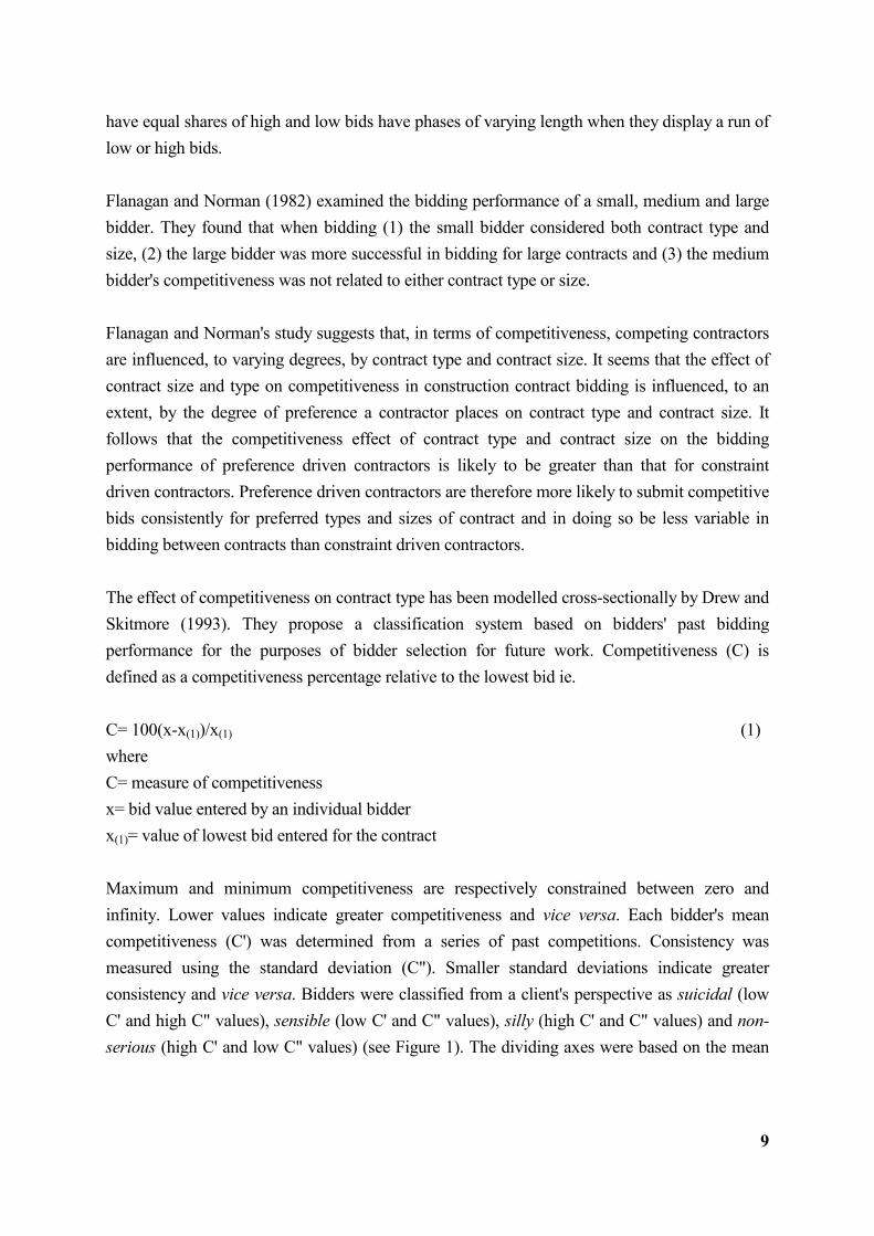
Flanagan and Norman (1982) examined the bidding performance of a small, medium and large

bidder. They found that when bidding (1) the small bidder considered both contract type and

size, (2) the large bidder was more successful in bidding for large contracts and (3) the medium

bidder's competitiveness was not related to either contract type or size.

Flanagan and Norman's study suggests that, in terms of competitiveness, competing contractors

are influenced, to varying degrees, by contract type and contract size. It seems that the effect of

contract size and type on competitiveness in construction contract bidding is influenced, to an

extent, by the degree of preference a contractor places on contract type and contract size. It

follows that the competitiveness effect of contract type and contract size on the bidding

performance of preference driven contractors is likely to be greater than that for constraint

driven contractors. Preference driven contractors are therefore more likely to submit competitive

bids consistently for preferred types and sizes of contract and in doing so be less variable in

bidding between contracts than constraint driven contractors.

The effect of competitiveness on contract type has been modelled cross-sectionally by Drew and

Skitmore (1993). They propose a classification system based on bidders' past bidding

performance for the purposes of bidder selection for future work. Competitiveness (C) is

defined as a competitiveness percentage relative to the lowest bid ie.

C= 100(x-x(1))/x(1) (1)

where

C= measure of competitiveness

x= bid value entered by an individual bidder

x(1)= value of lowest bid entered for the contract

Maximum and minimum competitiveness are respectively constrained between zero and

infinity. Lower values indicate greater competitiveness and vice versa. Each bidder's mean

competitiveness (C') was determined from a series of past competitions. Consistency was

measured using the standard deviation (C"). Smaller standard deviations indicate greater

consistency and vice versa. Bidders were classified from a client's perspective as suicidal (low

C' and high C" values), sensible (low C' and C" values), silly (high C' and C" values) and non-

serious (high C' and low C" values) (see Figure 1). The dividing axes were based on the mean

10

competitiveness (C') and standard deviation (C") of the bidders in the sample. Suicidal bidders

were found to rank the most competitive, followed by sensible and silly with non-serious being

the least competitive. The same classification system has also been applied to a study aimed at

analysing the influence of a contractor's competitors (Drew et al 1993).

A comprehensive approach to modelling competitiveness cross-sectionally between bids has

been introduced in the form of multiple regression analysis by Drew and Skitmore (1990, 1992)

who considered bidders' competitiveness in relation to contract type and contract size. This

paper extends this work through regression model building and offers a prediction equation

which relates bidders' competitiveness (the dependent variable) to the independent variables of

bidder, contract type and contract size.

METHODOLOGY

Since the study by Flanagan and Norman (1982) appears to be the closest study that examines

the variables of interest, this study has been used as the basis on which to develop the

methodology for this study.

Measuring competitiveness in bidding

Flanagan and Norman (1982) measured the competitiveness of each bidder in terms of success

rates and as a percentage relative to the bidder's bid. A measure of bid variability within the bid

distribution was determined by using the coefficient of variation resulting from the aggregate

mean percentage bidding range for each bidder. In developing Flanagan and Norman's study a

preferred alternative competitiveness measure is offered. Competitiveness (C) is measured by

the ratio of lowest bid to bidder's bid ie.

C =x(1)/x (2)

where

C= measure of competitiveness

x= bid value entered by an individual bidder

x(1)= value of lowest bid entered for the contract

Maximum and minimum competitiveness are respectively constrained between one and zero2.

2It should be noted that zero is a theoretical minimum. In reality no bidder would be able to obtain this value as

the bidder's bid would have to be approaching infinity.

11

This competitiveness measure has a number of advantages:

1. it is easy to calculate;

2. the scale is logarithmic (ie. the log of this variable will be the same as log x(1) - log x);

differences between the dependent variable become more pronounced nearer unity, the

end of the scale which is likely to be of greatest interest (ie. maximum competitiveness).

The logarithmic scale will also dampen any possible non-constant variance (non-

constant variance, or heteroscedasticity as it is otherwise known, constitutes a regression

assumption violation);

3. it is very adaptable to transformation; log transformations can be used since there will be

no zero values and arcsin transformations can be used since the scale is between one and

zero.

Development of the models

The model building process and selection of the best model is based on a chunkwise approach3.

Candidate models containing different chunk combinations of predictor variables were built and

the effect on competitiveness determined for each candidate model. The candidate models were

then systematically compared using a forward chunkwise sequential variable selection algorithm

based on the F test (see Appendix A for further details) to find the best model (ie. chunk

combination) that reflects competitiveness.

Candidate models contain both quantitative and qualitative independent variables4. Contract

size (S), a quantitative independent variable, has been expressed in terms of contract value. A

quadratic term for this variable was added to allow the regression line to reflect possible

economies of scale between contract size and bidder size. Relationships between

competitiveness and contract size can be observed by plotting the value of bids entered in past

competitions against the competitiveness measure (ie. Equation 2) with bidder's bid plotted at

the lowest bid value5. Curvilinear regression analysis can be used to determine the line of best

fit (eg. Figure 2).

3Detailed explanations of this approach can be found in most intermediate texts on regression analysis such as

Klienbaum, Kupper and Muller (1988) or Kelting (1979).

4See eg. Mendenhall and Sinich (1993) on regression analysis model building.

5The bid values that make up a bidding distribution, when plotted against competitiveness and contract size, will

follow a straight line relative to the lowest bid. If the bids are plotted according to each bid value, the angle of the

line will not be perpendicular. This is because smaller contracts produce greater ratio differences between values

12

Bidder (B) and contract type (T) are both qualitative variables. A single prediction equation for

each bidder and type can be found through the standard procedure of using dummy variables.

A chunk of predictor variables is required for each independent variable (ie. S, T, B). A chunk

of predictor variables is also required for each of the corresponding two-way interactions (ie.

ST, SB and TB) and three-way interaction (ie. STB). Candidate models comprising up to seven

chunks of predictor variables were, therefore, considered. A total of 22 candidate models has

been developed according to different chunk combinations. As can be seen from Figure 3, the

candidate models vary from the simplest model (model 1) based on the sample mean to a seven

chunk model (model 22) which is taken to be the saturated model.

Data set

Data from tender reports was collected from the Architectural Services Department of the Hong

Kong Government on the basis of Flanagan and Norman's study6 and classified according to the

CI/Sfb classification system (Ray-Jones and Clegg 1976) into five contract types (ie. fire

stations, police stations, primary schools, secondary schools and hostels). The data set

comprised 190 contracts made up of 2395 bidding attempts from 195 bidders for the period

1980-90. Each bidder was assigned a code to preserve anonymity. For comparison all contract

values were updated to a common base date (September 1990) based on the Hong Kong

Government tender price index for building work (Levett and Bailey 1990).

Number of bidders

Ideally as many bidders as possible should be included in the analysis. However, there are data

limitations and for reasonably robust results Skitmore (1991) recommends that the number of

previous bidding attempts is three times the number of variables in the model. To overcome this

(eg. a small contract which has a bid of $2 million and a lowest bid of $1 million will generate competitiveness of

0.5 for a contract size difference of $1 million; a large contract which has a bid of $110 million and the lowest bid of

$100 million will generate a competitiveness of 0.91 for a contract size difference of $10 million). The slopes of the

bidding distributions will, therefore, become progressively oblique as the contract size increases. To eliminate this sloping effect and maintain perpendicularity all bidding attempts need to be and have been plotted at the point of the

lowest bid.

6ie. all projects were (a) for one sector, the public sector, (b) were of similar building type: mainly primary and

secondary schools, fire and police stations and hostels, (c) were in the same geographical region, in this case Hong

Kong.

13

problem a standard procedure for this type of analysis is to select bidders with the most bidding

attempts. Bidders were ranked in descending order of bidding attempts and a cumulative

number of bidding attempts was determined. Against this was compared the corresponding

number of variables generated by the saturated model to find a reasonable minimum ratio cut

off point. For this data set this was judged to be where 15 bidders were included in the analysis

for which there were 776 bidding attempts.

Although the ratio at this point for model 22 (ie. the saturated model) was only 2.70 (ie. 776

bidding attempts / 287 variables), this was considered reasonable since this ratio is only just less

than three. Also, with the exception of two other models (ie. models 19 and 20), all other

candidate models have a ratio greater than three. It is quite likely, therefore, that the best

candidate model would in fact have a ratio greater than three.

ANALYSIS

The 22 candidate models were ranked for testing in ascending order of the number of explained

degrees of freedom and the best model found using the chunkwise approach. Model 12 was

found to be the best model (see Appendix A for further details). The robustness of the best

model was tested extensively. This included varying the combinations of bidders and contract

types, recalculating the F-test results at 1% significant level and examining whether the second

order terms contribute to the prediction of competitiveness.

The residuals of the best model were examined to see if any of the standard least squares

regression assumptions had been violated. Each assumption was examined in turn and, where

necessary, the model was modified to accommodate the assumption to produce a final model

which was not only closest to satisfying these assumptions but also the best predictor of the

dependent variable, competitiveness (see Appendix B for further details).

The best model, transformed to satisfy the regression assumptions, was subsequently retested

against all other candidate models to verify whether it remains in its modified state as the best

model (see Appendix C for further details).

The prediction equations from the best model were estimated and analyzed (see Appendix D for

equation details). This included testing the reliability of the model by constructing 95%

prediction intervals around the equations.

14

FINDINGS

Selection of the predictor variables

The selection of predictor variables was undertaken in two stages. The chunkwise algorithm

was used in the first stage to determine the best candidate model. Of the 22 candidate models,

model 12 was found to be the best model. This algorithm eliminated the two principal bidder-

contract type interaction variables (ie. TB and STB). The deletion of these variables indicates

that the contract type - bidder interactions (ie. TB) are less important than the other chunks

remaining in the model. When testing this model against the regression assumptions, it was

found that the model failed the regression assumptions of multicollinearity and

homoscedasticity and, therefore, required transforming.

Backwards stepwise regression was used in the second stage, as part of the correction process,

to reduce multicollinearity to an acceptable level. This eliminated all the insignificant variables

within each chunk and, thereby, reduced the total number of variables in the model from 56 to

24 significant variables. Consequently all the predictor variables were deleted for fire stations

and bidders coded 18, 109, 122, 127 and 148. Since the regression matrix is inverted on the last

set of dummy variables entered into the equation (in this instance, hostels and bidder coded 9),

the results indicate that bidders' competitiveness toward fire stations is not significantly different

from hostels and bidders 9, 18, 109, 122, 127 and 148 competitiveness is not significantly

different from each other.

By iterating the regression analysis on the last dummy variables of each and every contract type

and bidder, the backwards stepwise regression was also used to identify the other contract types

and bidders are not significantly different from each other. Since a fundamental goal of model

building is to find the best prediction model containing the least number of variables, those

contract types and bidders that were found not to be significantly different were combined in

subsequent iterations.

Of the five contract types, bidders' competitiveness towards three of the contract types was

found to be significantly different. The analysis also shows that the competitiveness of eight of

the 15 bidders to be significantly different from each other.

15

Model utility statistics

After completing the selection of predictor variables the model's utility was examined. The

global F test statistics were found to be significant (F.05 = 13.05, p = .0000, df= 21, 754). This

means that at least one of the model coefficients is non-zero and, therefore, the model is useful

at predicting competitiveness. The model achieves an adjusted R square statistic of 0.25369

which indicates that approximately 25% of competitiveness variation is explained by the model.

With the aid of a standard spreadsheet software package the competitiveness prediction

equations were estimated for each bidder according to each contract type (see Appendix D for

equation details).

Contract type and size

The five original contract types were pooled into the three significantly different

competitiveness groupings of (1) fire stations and hostels, (2) police stations and secondary

schools and (3) primary schools. It seems the formation of these groupings primarily is

influenced by the different means and distribution of contract sizes for each contract type which

appear to fall into three contract size bands. Primary schools had the smallest mean bid value

and standard deviation and in ascending rank order this was followed by fire stations and

hostels, police stations and secondary schools (see Table 1).

Figure 4 a - c show the competitiveness predictions for each of the bidders according to the

three contract type groupings. Bold lines indicate the fit within the recorded data values and

dashed lines show the curve extrapolated outside the data values. In respect of the shape of the

curves for (1) fire stations and hostels and (2) police stations and secondary schools it can be

seen that four lines the are the expected convex shape (which indicates the bidders have a

preferred contract size), two are concave and one line is straight and horizontal. The straight and

horizontal line represents the competitiveness of the six bidders whose competitiveness is not

significantly different from each other. The reason for the straight and horizontal line is that all

the coefficients except the constant have been deleted from the equation. The horizontal line

suggests that the competitiveness of these bidders is unaffected by contract size.

Although the level of competitiveness, slope and degree of curvature of the regression lines for

the three groups of types are significantly different the overall shape of the regression lines for

(1) fire stations and hostels and (2) police stations and secondary schools are somewhat similar

16

in shape. The likely reason for this similarity is that in using the chunkwise algorithm the major

contract type - bidder interaction chunks (ie. TB and STB) are deleted from the equation and

that both of these type groupings contain both smaller and larger contracts. Of these two types

bidders appear to be more competitive toward police stations and secondary schools. The

apparent difference may be explained by the fact that there are a greater number of larger police

station and secondary school contracts than fire station and hostel contracts. Thus it is apparent

that bidders are more competitive on larger contracts than smaller contracts.

For primary schools all 15 bidders displayed the expected convex shape. A major difference

between primary schools and the other four contract types is the range and distribution of

contract sizes. The data sets for the other four contract types are made up of a wider, more

evenly distributed range of contract sizes whereas the majority of primary school contracts fall

into a very narrow, concentrated band. The probable reason why all 15 curves are concave in

shape is due to the make up of this particular sample in which nearly all of the primary schools

are of a standard size. It appears that because the contract is a standard size, bidders from past

experience can be more confident in predicting what the market price is likely to be and bid

accordingly, thereby making the bids between bidders less variable and more competitive. An

important contributory factor to this is that the sample for this type also contained a few smaller

alteration contracts and a few larger primary school contracts in which the bids are more

variable and overall less competitive. It seems that the combination of the wider dispersion of

bids for the smaller alteration work and larger primary school contracts combined with the

narrower dispersion of bids for the standard new work primary school contracts has produced

convex curves for every bidder.

Individual bidder performance

The same competitiveness predictions for the three pooled contract types were regrouped

according to the eight pooled bidders (see Figure 5 a - h).

The 15 bidders appear to fall into five distinct competitiveness groupings:

1. bidders who, in terms of competitiveness, have a preferred contract size range for

smaller contracts (ie. bidders 52 and 96);

2. bidders who, in terms of competitiveness, have a preferred contract size range for larger

contracts (ie. bidders 20, 24, 69, 119);

3. bidders who are more competitive on the larger contracts (ie. bidders 71 and 142);

17

4. bidders whose competitiveness is, largely, unaffected by contract size (ie. bidders 9, 18,

109, 122, 127 and 148);

5. bidders who are less competitive on larger contracts (ie. bidder 45).

The distinction between (3) and (4) is in the shape of the competitiveness curves which are

convex and concave respectively.

In considering the bidding performances of bidders who fall into the same competitiveness

grouping but whose competitiveness performance is significantly different it can be seen that of

the two contractors who have a preferred contract size range for smaller contracts bidder 96 is

shown to be significantly more competitive than 52. Likewise of the contractors who have a

preferred contract range for larger contracts, bidders 20, 69 and 119 are shown to be

significantly more competitive than 24. In respect of the two bidders who are more competitive

on the larger contracts the essential difference seems to be that bidder 71 is more competitive

than bidder 142 at the smaller end of the contract size continuum whereas bidder 142 is more

competitive at the larger end of the contract size continuum.

The results provide evidence that three pooled contract types are part of the same market sector

since it is the same bidders who have preferred contract sizes for the smaller contracts in all

groupings. It seems those bidders who have a preferred contract size range for larger contracts

or are more competitive towards larger contracts are not competitive toward primary schools

simply because there are no large contract sizes pertaining to this type.

The bidding performances of five other bidders were examined also to see if other

competitiveness groupings could be found. No new groupings were identified.

Reliability

The reliability of the model was examined by comparing the predicted values with the 95%

upper and lower prediction intervals according to contract type and bidder.

A representative sample from the five competitiveness groupings comprising bidders 96, 69, 71,

45 and the six pooled bidders (ie. bidders 9, 18, 109, 122, 127 and 148) for (1) primary and (2)

secondary schools is shown in Figure 6. This figure shows a scatterplot of the predicted values

(denoted by squares), 95% upper and lower prediction intervals (respectively denoted by

diamonds and triangles) and actual bidding attempts (denoted by crosses). Due to the

18

logarithmic nature of the scale, the upper and lower confidence intervals are not equidistant

from the predicted values. As expected, the distances between the predictions and confidence

intervals form a relatively wide band which signifies that the competitiveness predictions are

not very reliable.

Despite the competitiveness predictions not being very reliable, Figure 6 does show which

bidders are likely to have the potential for submitting the lowest bid; this can be observed by

comparing the 95% upper interval predictions with the competitiveness value of unity (ie.

equivalent to the lowest bid). If the upper interval prediction falls directly on a competitiveness

value of unity (ie. equivalent to the lowest bid) then it is predicted that the bidder has a 1 in 20

chance of submitting the lowest bid. If this interval prediction is greater than unity then this

probability increases and vice versa.

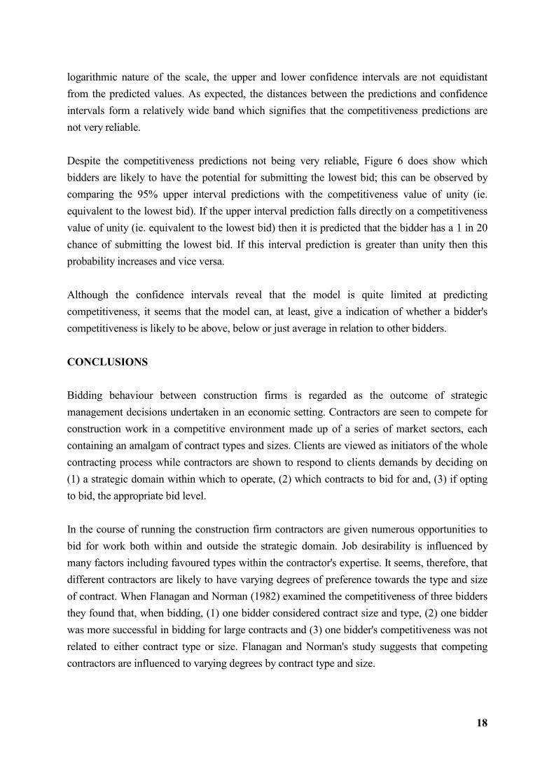
Although the confidence intervals reveal that the model is quite limited at predicting

competitiveness, it seems that the model can, at least, give a indication of whether a bidder's

competitiveness is likely to be above, below or just average in relation to other bidders.

CONCLUSIONS

Bidding behaviour between construction firms is regarded as the outcome of strategic

management decisions undertaken in an economic setting. Contractors are seen to compete for

construction work in a competitive environment made up of a series of market sectors, each

containing an amalgam of contract types and sizes. Clients are viewed as initiators of the whole

contracting process while contractors are shown to respond to clients demands by deciding on

(1) a strategic domain within which to operate, (2) which contracts to bid for and, (3) if opting

to bid, the appropriate bid level.

In the course of running the construction firm contractors are given numerous opportunities to

bid for work both within and outside the strategic domain. Job desirability is influenced by

many factors including favoured types within the contractor's expertise. It seems, therefore, that

different contractors are likely to have varying degrees of preference towards the type and size

of contract. When Flanagan and Norman (1982) examined the competitiveness of three bidders

they found that, when bidding, (1) one bidder considered contract size and type, (2) one bidder

was more successful in bidding for large contracts and (3) one bidder's competitiveness was not

related to either contract type or size. Flanagan and Norman's study suggests that competing

contractors are influenced to varying degrees by contract type and size.

19

To measure the effect of contract type and contract size on competitiveness in bidding, 15

bidders were selected for analysis on the basis of most bidding attempts and a suitable

regression methodology developed. 22 candidate models were proposed and the best model

found using a forward chunkwise sequential variable algorithm based on the F-test. Model 12

was found to be the best model and the robustness of this model was tested extensively before

transforming the model to satisfy the regression assumptions. The best model, transformed to

satisfy the regression assumptions, was retested against other transformed candidate models and

was found still to be the best model. The prediction equations were then estimated and the

reliability of the model tested by checking the coefficients and constructing 95% prediction

intervals around the prediction equations.

Although Flanagan and Norman's findings neatly link together the variables of contract type and

contract size, there is no indication of the relative effect of these relationships. The regression

model in this analysis not only shows this effect but also provides a powerful technique for

predicting competitiveness and testing the reliability of the competitiveness predictions. The

best model is found to be statistically useful as indicated by the global F test statistics (F.05 =

13.55, p = .0000, df= 21, 754) and adjusted R square statistic of 0.25369.

The analysis in this paper demonstrates that, in terms of competitiveness, contract size is more

important than contract type. Evidence of this can be seen by reviewing the findings, first, in the

predictor selection process and second, in the competitiveness predictions themselves.

The selection of predictor variables was undertaken in two stages. The chunkwise approach

eliminated the two principal bidder-contract type interaction variables (ie. TB and STB). The

deletion of these variables indicates that the contract type -bidder interactions are less important

than the contract size interactions (ie. ST and SB).

Backwards stepwise regression eliminated the insignificant variables remaining in the equation.

In using backwards stepwise regression and iterating the regression model on the last dummy

variable of each contract type, it was found that bidders' competitiveness did not differ

significantly between fire stations and hostels nor between police stations and secondary

schools. The original five contract types were, therefore, grouped into the three significantly

different competitiveness groupings of (1) fire stations and hostels, (2) police stations and

secondary schools and (3) primary schools. It seems the formation of these groupings is

influenced by the different means and distribution of contract sizes for each contract type which

20

fall into three contract size bands. Primary schools had the smallest mean bid value and standard

deviation and, in ascending rank order, were followed by fire stations and hostels, police

stations and secondary schools.

Of the five contract types, competitiveness towards primary schools appeared to differ the most.

A major factor is that the sample of primary schools does not contain any large contracts and,

judging by the narrow distribution of bid values, is highly standardised in terms of contract size.

This standardisation has lead to an increase in bidders' competitiveness towards this type when

compared with other types. The results provide evidence that bidders are more competitive

toward police stations and secondary schools than fire station and hostel contracts. The

difference can be explained by the fact that there are a greater number of larger police station

and secondary school contracts than fire station and hostel contracts. This signifies that bidders

are more competitive on larger contracts than on smaller contracts.

These findings indicate that bidders' competitiveness towards a contract type is affected by (1)

the degree of contract type standardisation and (2) the sizes of contract contained within a

contract type. The greater the degree of contract type standardisation and the larger the sizes of

contract within a contract type, the greater the likely competitiveness of bidders towards the

contract type and vice versa.

The three contract type groupings would seem to be part of the same market sector since it is the

same bidders who have preferred contract sizes for the smaller contracts in all groupings. It

seems those bidders who have a preferred contract size range for larger contracts, or are more

competitive towards larger contracts, are not competitive toward primary schools simply

because there are no large contract sizes pertaining to this type. Perhaps it is not surprising to

find that contract size is more important than contract type in this analysis, since a Flanagan and

Norman criterion (Flanagan and Norman 1982) was that the data was made up of similar

contract types.

Of the 15 bidders, eight were found to be significantly different in terms of competitiveness.

The notion that bidders have preferred size ranges at which they are more competitive appears

to hold as the shape of regression lines are, mostly, the expected convex shape. The exceptions

tend to be with bidders who are less competitive. The effect of contract size on bidder's

competitiveness varies considerably between some bidders. The analysis shows that the 15

bidders can be classified into five distinct competitiveness groupings:

21

1. bidders who, in terms of competitiveness, have a preferred contract size range for

smaller contracts (ie. bidders 52 and 96);

2. bidders who, in terms of competitiveness, have a preferred contract size range for larger

contracts (ie. bidders 20, 24, 69, 119);

3. bidders who are more competitive on the larger contracts (ie. bidders 71 and 142);

4. bidders who are less competitive on larger contracts (ie. bidder 45);

5. bidders whose competitiveness is largely unaffected by contract size (ie. bidders 9, 18,

109, 122, 127 and 148);

The distinction between (3) and (4) is in the shape of the competitiveness curves which are

convex and concave respectively. A simplified representation of these five competitiveness

groupings is shown in Figure 7. With the exception of bidder groupings (4) and (5), the shapes

of the competitiveness lines are shown as convex. This conforms to the notion that bidders have

a preferred contract size at which they are more competitive.

In addition to the 15 bidders, the bidding performances of five other bidders were examined to

see if other competitiveness groupings could be found. No new groupings could be identified.

Flanagan and Norman (1982) found that one bidder was more competitive on larger contracts

while another bidder's competitiveness was, largely, unaffected by contract size. Bidders

displaying the same characteristics are found in this analysis ie. in groups (3) and (5). In

addition, it can be seen that three new competitiveness groupings are identified ie. (1), (2) and

(4). The most competitive bidders appear to be those who have preferred contract sizes, either

for smaller or larger contracts ie. those bidders who appear in groups (1) and (2).

Flanagan and Norman (1982) also concluded that one of the bidders they analysed was

influenced by both contract size and type. However, the relative influence of contract size and

type was not reported. The analysis in this paper indicates that contract size is more influential

than contract type. A suggested reason why contract type differences do not influence

competitiveness greatly is that all the five contract types are from the same market sector.

The results indicate that contractors, in terms of competitiveness, are influenced to varying

degrees by contract size and contract type. Although the 95% prediction intervals reveal that the

model is somewhat limited at predicting competitiveness, the best model does, at least, give an

indication of whether a bidder's competitiveness is likely to be above, below or average in

relation to other bidders.

22

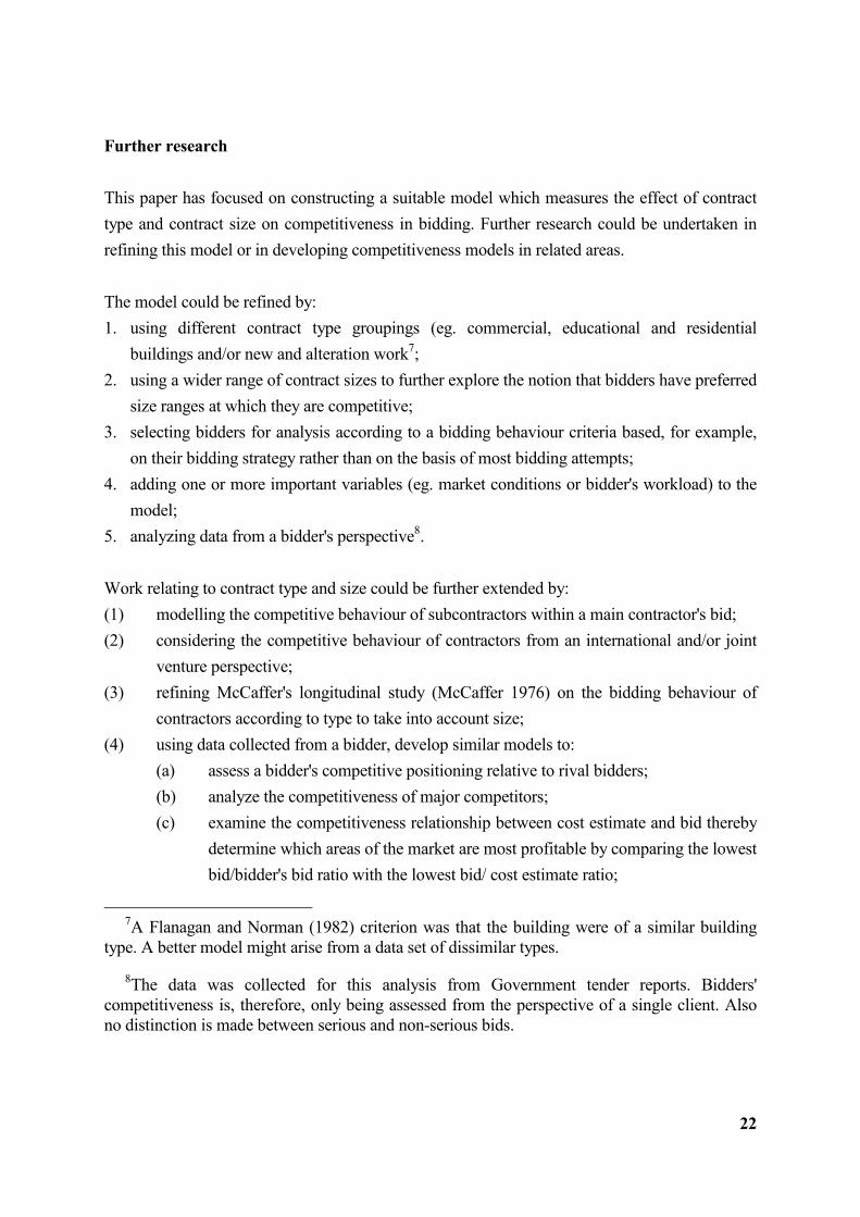
Further research

This paper has focused on constructing a suitable model which measures the effect of contract

type and contract size on competitiveness in bidding. Further research could be undertaken in

refining this model or in developing competitiveness models in related areas.

The model could be refined by:

1. using different contract type groupings (eg. commercial, educational and residential

buildings and/or new and alteration work7;

2. using a wider range of contract sizes to further explore the notion that bidders have preferred

size ranges at which they are competitive;

3. selecting bidders for analysis according to a bidding behaviour criteria based, for example,

on their bidding strategy rather than on the basis of most bidding attempts;

4. adding one or more important variables (eg. market conditions or bidder's workload) to the

model;

5. analyzing data from a bidder's perspective8.

Work relating to contract type and size could be further extended by:

(1) modelling the competitive behaviour of subcontractors within a main contractor's bid;

(2) considering the competitive behaviour of contractors from an international and/or joint

venture perspective;

(3) refining McCaffer's longitudinal study (McCaffer 1976) on the bidding behaviour of

contractors according to type to take into account size;

(4) using data collected from a bidder, develop similar models to:

(a) assess a bidder's competitive positioning relative to rival bidders;

(b) analyze the competitiveness of major competitors;

(c) examine the competitiveness relationship between cost estimate and bid thereby

determine which areas of the market are most profitable by comparing the lowest

bid/bidder's bid ratio with the lowest bid/ cost estimate ratio;

7A Flanagan and Norman (1982) criterion was that the building were of a similar building type. A better model might arise from a data set of dissimilar types.

8The data was collected for this analysis from Government tender reports. Bidders' competitiveness is, therefore, only being assessed from the perspective of a single client. Also no distinction is made between serious and non-serious bids.

23

(d) extend (4)(c) to determine mark-up levels for future projects.

The notion that bidders have a range of preferred contract sizes could be explored further by

comparing:

(1) the individual and grouped competitive behaviour of bidders in terms of bidder size (eg.

small, medium or large);

(2) the different measures of bidder size (eg. turnover, no. of employees and market share)

24

REFERENCES

Bannock G., Baxter R.E. and Davis, E. (1987) Dictionary of economics, 4th edition, Penguin

Books, London.

Beeston, D.T. (1983) Statistical methods for building price data, E & FN Spon, London.

Benjamin, N.B.H. (1969) Competitive bidding for building construction contracts, PhD

dissertation, Stanford University.

Briscoe, G. (1988) The economics of the construction industry, Mitchell, London.

Cannon, J. and Hillebrandt, P.M. (1989) Theories of the firm, In The Management of

Construction Firms: Aspects of Theory (edited by Hillebrandt P.M. and Cannon J.) Macmillan,

London, 1-7.

Cook, A.E. (1991) Construction Tendering, B.T. Batsford Ltd., London.

Cryer, J.D. and Miller, R.B. (1991) Statistics of business: data analysis and modelling, PWS-

Kent Publishing Company, Boston.

Davis, Langdon and Seah International (1994) Asia Pacific construction costs handbook, E &

FN Spon, London.

Dielman, T.E. (1991) Applied regression analysis for business and economics, PWS-Kent

Publishing Company, Boston.

Drew, D.S. and Skitmore, R.M. (1990) Analysing bidding performance; measuring the

influence of contract size and type, Building Economics and Construction Management;

Management of the building firm, International Council of Construction Research Studies and

Documentation, CIB W-65 Sydney, Australia, 129-39.

Drew, D.S. and Skitmore, R.M. (1992) Competitiveness in bidding: a consultant's perspective,

Construction Management and Economics, 10, 227-47.

25

Drew, D.S. and Skitmore, R.M. (1993) Prequalification and C-competitiveness, OMEGA

International Journal of Management Science, 21, 363-75.

Drew, D.S., Skitmore, R.M. and Lo, H.P. (1993) Competitiveness in bidding: analysing the

influence of competitors, Organisation and management of construction - the way forward,

International Council of Construction Research Studies and Documentation, CIB W-65 Port of

Spain, Trinidad, 417-26.

Fine, B. (1975) Tendering Strategy, Aspects of the economics of construction, In Turin D.A.

(ed), Godwin, 203-221.

Flanagan, R. and Norman, G. (1982) An examination of the tendering pattern of individual

building contractors, Building Technology and Management 28 (April), 25-28.

Flanagan, R. and Norman, G. (1985) Sealed bid auctions: an application to the building

industry, Construction Management and Economics, 3, 145-61.

Friedman, L. (1956) A competitive bidding strategy, Operations Research, 1 (4), 104-12.

Griffith, A. (1992) Small building works management, Macmillan, Basingstoke.

Hillebrandt, P.M. (1985) Economic theory and the construction industry, 2nd edition,

Macmillan, Basingstoke.

Hillebrandt, P.M. and Cannon, J. (1990) The modern construction firm, Macmillan, London.

Johnson, G.J. and Scholes, K. (1993) Exploring corporate strategy, Third Edition, Prentice-Hall

International, Hemel Hempstead.

Kast, F.E. and Rosenzweig, J.E. (1985) Organisation and management: a systems and

contingency approach, Fourth Edition, McGraw-Hill, New York.

Kelting, H. (1979) An investigation of factors affecting the sale of condominium units, In A

second course in business statistics by Mendenhall W. and Sinich T., Third edition, 1989.

Dellen Publishing Company, San Francisco 655-79

26

Kenkel, J.L. (1989) Introductory statistics for management and economics, Third edition, PWS-

Kent Publishing Company, Boston.

Klienbaum, D.G., Kupper, L.L. and Muller, K.E. (1988) Applied regression analysis and other

multivariate methods, PWS-Kent Publishing Company, Boston.

Langford, D.A. and Male, S. (1991) Strategic management in construction, Gower, Aldershot.

Lansley, P. Quince, T. and Lea, E. (1979) Flexibility and efficiency in construction

management, The final Report on a research project with financial support of the DoE. Building

Industry Group, Ashbridge Management Research Unit (unpublished)

Levett and Bailey (1990) Tender price indices, 1990, Levett and Bailey, Hong Kong.

Male, S. (1991a) Strategic management for competitive strategy and advantage, In Male S. and

Stocks R. (eds.), Competitive advantage in construction, Butterworth - Heinemann Ltd.,

Oxford, 1-4.

Male, S. (1991b) Strategic management in construction: conceptual foundations, In Male S. and

Stocks R. (eds.), Competitive advantage in construction, Butterworth - Heinemann Ltd.,

Oxford, 5-44.

McCaffer, R. (1976) Contractors' bidding behaviour and tender price prediction, PhD thesis,

Loughborough University of Technology.

Mendenhall, W. and Sinich, T. (1993) A second course in business statistics: regresssion

analysis, Fourth Edition, Macmillan Publishing Company, New York.

Merna, A. and Smith, N.J. (1990) Bid evaluation for UK public sector construction contracts, In

Proceedings, Institution of Civil Engineers, Part 1, 88 (Feb.), 91-105

Neter, J., Wasserman, W. and Kutner, M.H. (1983) Applied linear regression models, Irwin,

Homewood, Illinois.

Newcombe, R. (1976) The evolution and structure of the construction firm, MSc Thesis,

University College, London.

27

Newcombe, R., Langford, D. and Fellows R. (1990) Construction Management 1 :

Organisation Systems, Mitchell, London.

Odusote, O.O. and Fellows, R.F. (1992) An examination of the importance of resource

considerations when contractors make project selection decisions, Construction Management

and Economics, 10, 137-51.

Pearce, J.A. and Robinson, R.B. (1991) Strategic management practice, Irwin, Boston.

Ray-Jones, A. and Clegg, D. (1976) CI/SfB Construction Indexing Manual, 3rd Revised edition,

RIBA Publications Ltd, London.

Schweizer, U. and Ungern-Sternberg, T.V. (1983) Sealed bid auction and the search for better

information, Econometrica 50, 79-86.

Shepherd, W.G. (1990) The economics of industrial organization, Prentice-Hall International,

Englewood Cliffs, New Jersey.

Skitmore, R.M. (1981) Why do tenders vary?, Chartered Quantity Surveyor, 4, 128-9.

Skitmore, R.M. (1982) A bidding model, Building cost techniques: new directions, In Brandon

P.S. (ed.), E & FN Spon, London, 278-289.

Skitmore, R.M. (1988) Fundamental research in bidding for estimating, Paper presented to the

International Council for Construction Research Studies and Documentation CIB W-55, Haifa,

Israel.

Skitmore, R.M. (1989) Contract Bidding in Construction, Longman, Harlow.

Skitmore, R.M. (1991) Contract price forecasting and bidding strategies, In Brandon, P S (ed.)

Quantity surveying techniques; new directions, BSP Professional Books, Oxford.

Stone, P.A. (1983) Building Economy, Pergamon Press, Oxford.

28

APPENDIX A: SELECTING THE BEST MODEL

The approach used in determining the best model was by using a forward chunkwise sequential

variable selection algorithm based on comparing the calculated F statistic expressed in terms of

the sums of squares error as:

F(DA,DB,) =[SSEA - SSEB]/(da - db)/MSQB

where

SSEA = Sum of Square Error for model A

SSEB = Sum of Square Error for model B

da = Explained degrees of freedom for model A

db = Explained degrees of freedom for model B

MSQ = Mean square residual error for model B

with the corresponding tabulated F distribution at the 5% significance level

where

n1 = da - db degrees of freedom

n2 = residual degrees of freedom

When comparing models the null hypothesis is that the model with the explained degrees of

freedom is the best model. If the resulting calculated value for the F statistic exceeds the

tabulated F distribution at the 5% significance level then null hypothesis is rejected and the best

model then becomes the model represented in the alternative hypothesis. In the case where the

compared models contain an identical number of coefficients then the model with the smallest

SSE (sum of squared error) is automatically chosen as the best model. This algorithm is

repeated until all the models have been compared.

Model 12 was found to be the best model using the forward chunkwise sequential variable

selection algorithm. To use this algorithm the explained and residual df, SSE and MS Error

needed to be calculated for each of the candidate models. The candidate models were then

ranked in order of explained df. A summary of these statistics for each of the 22 candidate

models according to the 5 contract types and 15 bidders is given in Table 2. Table 3 shows the

resulting tabulated and calculated F values after applying the chunkwise algorithm to the Table

2 statistics.

29

APPENDIX B: SATISFYING THE REGRESSION ASSUMPTIONS

The variance inflation factors (VIFs) for the individual B parameters were used to detect

multicollinearity9. With regard to autocorrelation, in bidding studies where bidders who have

bid for the same contract are being analyzed the potential problem of `artificial' autocorrelation

is likely to occur if the data set is arranged chronologically. The chronological order for

contracts containing more than one bidding attempt will produce clusters similar value bids. The

clustering effect produces artificial dependency between succeeding bid values for the same

contract within the data set. This is likely to result in a significant autocorrelation. To minimise

this undesirable effect the ordering of the bid values within the data set is, therefore, randomised

at the commencement of the analysis. By randomising the data it can be regarded as being cross-

sectional. As autocorrelation in cross-sectional studies is `typically not an assumption of

concern' (Dielman 1991), the testing of this assumption was not reported.

The normality aspect is formally tested using the Kolmogorov-Smirnov test (see eg. Kenkel

1989) and verified using a normal probability plot. The assumption of homoscedasticity is also

formally tested. Each continuous and categorical variable in the model is respectively tested

using Szroeter's test (see eg. Dielman 1991) and Bartlett Box F test. This was verified by

observing a scatterplot of the studentised residuals against the predicted values.

The regression assumptions of multicollinearity, normality and homoscedasticity were tested for

possible violations. Using a combination of centring the x-variable, deleting insignificant

variables using backwards stepwise regression and transforming the x-variable based on the

exponential 2/3, model 12 is able to satisfy all of the regression assumptions except that of

homoscedasticity. It was found that 12 out of 26 variables were significantly heteroscedastic.

When applying the various Box-Cox transformations (see eg. Cryer and Miller, 1991) on a `trial

and error' basis to the selected model it was determined that the transformation that best

satisfied the homoscedasticity assumption was where lambda is set at -4.2. Three out of the 24

remaining independent variables were found to be significant. Ideally with 24 variables

remaining in the equation, at a 5% level of significance, it is expected that on average one or

two should be heteroscedastic. However, it is still admissible to have three significantly

heteroscedastic variables out of a total of 24 variables since the combined probabilities of the

three heteroscedastic variables out of 24 exceeds 5% level of significance. The probability of

obtaining three out of 24 variables being significantly heteroscedastic is:

9Severe multicollinearity is assumed to exist if the largest VIF is greater than 10 (Neter et al, 1983)

30

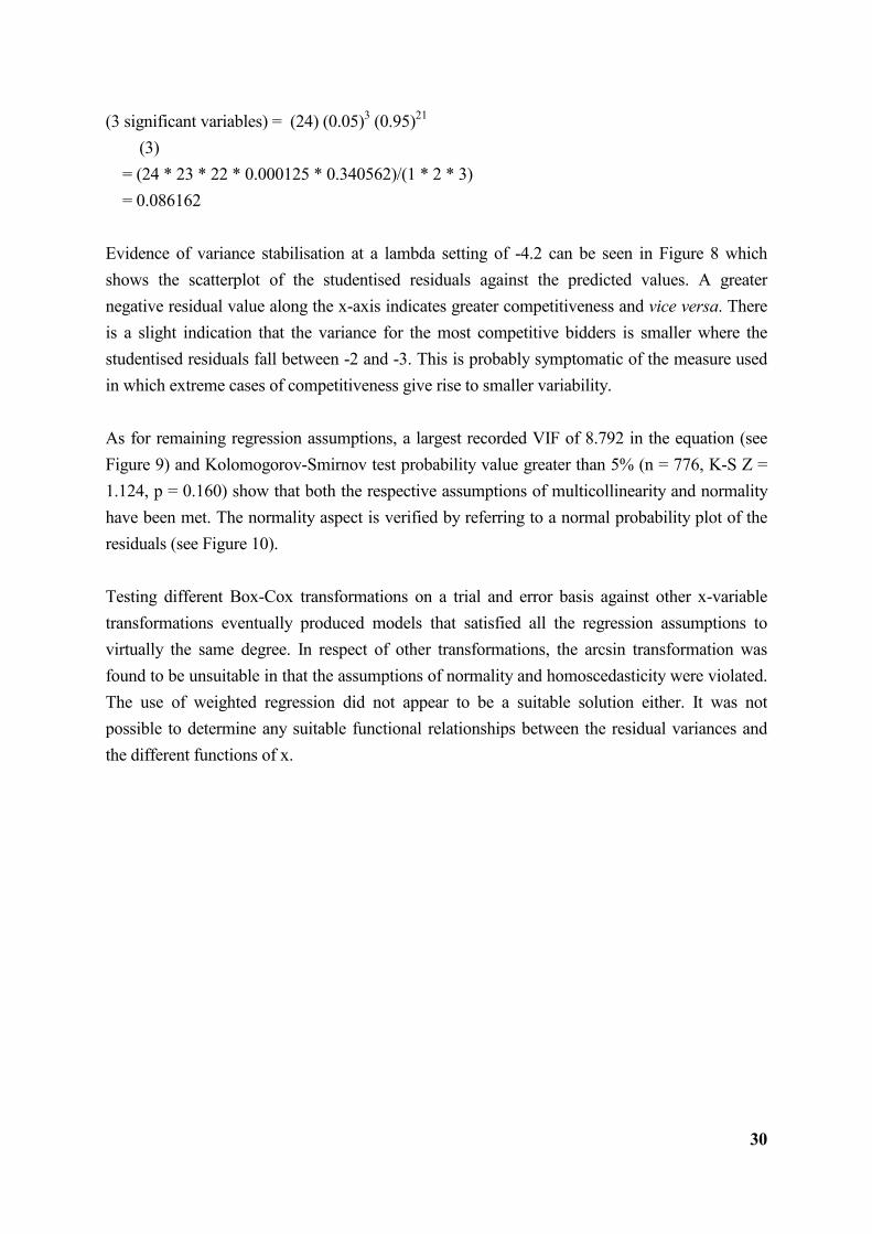
(3 significant variables) = (24) (0.05)3 (0.95)21

(3)

= (24 * 23 * 22 * 0.000125 * 0.340562)/(1 * 2 * 3)

= 0.086162

Evidence of variance stabilisation at a lambda setting of -4.2 can be seen in Figure 8 which

shows the scatterplot of the studentised residuals against the predicted values. A greater

negative residual value along the x-axis indicates greater competitiveness and vice versa. There

is a slight indication that the variance for the most competitive bidders is smaller where the

studentised residuals fall between -2 and -3. This is probably symptomatic of the measure used

in which extreme cases of competitiveness give rise to smaller variability.

As for remaining regression assumptions, a largest recorded VIF of 8.792 in the equation (see

Figure 9) and Kolomogorov-Smirnov test probability value greater than 5% (n = 776, K-S Z =

1.124, p = 0.160) show that both the respective assumptions of multicollinearity and normality

have been met. The normality aspect is verified by referring to a normal probability plot of the

residuals (see Figure 10).

Testing different Box-Cox transformations on a trial and error basis against other x-variable

transformations eventually produced models that satisfied all the regression assumptions to

virtually the same degree. In respect of other transformations, the arcsin transformation was

found to be unsuitable in that the assumptions of normality and homoscedasticity were violated.

The use of weighted regression did not appear to be a suitable solution either. It was not

possible to determine any suitable functional relationships between the residual variances and

the different functions of x.

31

APPENDIX C: VERIFYING THE BEST MODEL

To verify that model 12 in its transformed state remains as the best model, ideally each and

every candidate model needs to first be transformed in such a way that it satisfies all the

regression assumptions. However, the `trial and error' approach taken to satisfy the assumptions

is very time-consuming and time constraints make it impractical to attempt to transform every

model. Attempts were made, therefore, to transform the closest challengers to model 12 (ie.

models 18 and 21). However, suitable transformations to reduce multicollinearity to an

acceptable level for either model could not be found. Hence, the approach taken in the

verification process has been to analyze all other candidate models using the same

transformation that was used for model 12.

In testing the transformed model 12 against all other candidate models to verify whether model

12 in its transformed state remains as the best model, all variables, rather than just the

significant variables, were retained within the transformed candidate models. This approach is

taken due to the rationale underlying the chunkwise model building process ie. candidate

models have been built and analyzed on the basis of collective groups (or chunks) of variables

in preference to using individual significant variables.

32

APPENDIX D: MODEL PREDICTION

The prediction equation, transformed to suit the regression assumptions, is as follows:

_ = [(-4.2) [ a + b1 (x2/3-7.68) + b2 (x

2/3-7.68)2

+ b3T1 + b4T2 + ... bnTn + b5B1 + b6B1 + ... bnTn

+ b7T1 (x2/3-7.68) + b8T1 (x

2/3-7.68)2 ... + bnTn (x2/3-7.68) + bnTn (x

2/3-7.68)2

+ b9B1 (x2/3-7.68) + b10B1 (x

2/3-7.68)2 ... + bnBn (x2/3-7.68) + bnBn (x

2/3-7.68)2] +1]-1/4.2

where

_ = predicted competitiveness

x = contract size

T = contract type

B = bidder

Figure 9 illustrates the computer generated output relating to the transformed model. The

coefficients of these variables are given in the in the B column under the section of `Variables in

the Equation'.

33

Figure 1:Classification of bidders according to competitiveness and consistency in bidding

34

Figure 2:Competitiveness and contract size

35

Model

No.

No. of Chunks in

Model

Chunk Combination

1

2

3

4

5

6

7

8

9

10

11

12

13

14

15

16

17

18

19

20

21

22

0

1

2

2

3

3

3

4

4

4

4

5

5

5

5

5

5

6

6

6

6

7

y

S

S + T

S + B

S + T + ST

S + B + SB

S + T + B

S + T + B + ST

S + T + B + SB

S + T + B + TB

S + T + B + STB

S + T + B + ST + SB

S + T + B + SB + TB

S + T + B + TB + ST

S + T + B + STB + ST

S + T + B + STB + SB

S + T + B + STB + TB

S + T + B + SB + ST + STB

S + T + B + SB + BT + STB

S + T + B + BT + ST + STB

S + T + B + BT + SB + ST

S + T + B + BT + SB + ST + STB

where :

y = sample meanT = contract type

S = contract sizeB = bidder

The regression coefficients contained within these chunks are as follows:

1.S:b1x + b2x2

2.T:b3T1 + b4T2 ... bnTn

3.B:b5B1 + b6B2 ... bnBn

4.ST:b7T1x + b8T1x2 + b9T2x + b10T2x

2 ... bnTnx + bnTnx2

36

5.SB:b11B1x + b12B1x2 + b13B2x + b14B2x

2 ... bnBnx + bnBnx2

6.TB:b15B1T1 + b16B2T1 + b17B1T2 + b18B2T2 ... bnBnTn

7.STB:b19B1T1x + b20B1T1x2 + b21B2T1x + b22B2T1x

2 + b23B1T2x

b24B1T2x2 + b25B2T2x + b26B2T2x

2 + ... bnBnTnx + bnBnTnx2

where :

x = contract sizeT1 = contract type 1B1 = bidder 1

T2 = contract type 2B2 = bidder 2

Tn = contract type nBn = bidder n

Figure 3: Proposed candidate models

37

38

Figure 4:Competitiveness prediction models according to contract type

39

40

Figure 5:Competitiveness prediction models according to bidder

41

42

Figure 6:Scatterplot of the 95% upper and lower prediction intervals, predicted values and

actual bidding attempts according to bidder

43

Figure 7:Simplified representation of competitiveness groupings

44

Figure 8:Scatterplot of studentised residuals against the predicted values

45

* * * * M U L T I P L E R E G R E S S I O N * * * *

Equation Number 1 Dependent Variable .. DEP

Variable(s) Removed on Step Number

37.. B1BID2

Multiple R .52337

R Square .27392

Adjusted R Square .25369

Standard Error .05091

Analysis of Variance

DF Sum of Squares Mean Square

Regression 21 .73727 .03511

Residual 754 1.95432 .00259

F = 13.54519 Signif F = .0000

------------------------------------------------ Variables in the Equation -----------------------------------------

Variable B SE B Beta Tolerance VIF

J2BID2 .003906 9.0375E-04 .305869 .192297 5.200

B6BID .006639 .003482 .087418 .458021 2.183

B4BID .008388 .003465 .123593 .369494 2.706

B2 .054024 .010120 .209863 .623056 1.605

B5BID2 .001369 6.6094E-04 .090630 .502894 1.988

B3 .045184 .008532 .209540 .615057 1.626

B7 .043526 .011626 .179754 .417727 2.394

B1BID - .004733 .001009 -.154231 .891480 1.122

J1 - .011910 .004314 -.099153 .746465 1.340

B7BID .005666 .002028 .104357 .689836 1.450

B2BID - .008636 .002279 -.149086 .622063 1.608

B6 - .048907 .010811 -.201977 .483113 2.070

J2 - .024061 .009034 -.150185 .302876 3.302

J1BID - .003782 9.1729E-04 -.201389 .403524 2.478

B5 - .028459 .010364 -.120823 .497360 2.011

B7BID2 - .001120 3.9312E-04 -.128780 .471308 2.122

B6BID2 .002351 8.5783E-04 .136848 .386143 2.590

B3BID2 -7.91501E-04 4.0932E-04 -.076160 .620797 1.611

B4 .076707 .011999 .325666 .371063 2.695

J1BID2 1.78966E-04 6.7822E-05 .118438 .478003 2.092

J2BID .011411 .005408 .194122 .113744 8.792

(Constant) .103502 .003314

Figure 9:Regression model summary

46

Figure 10: Normality probability plot of the residuals

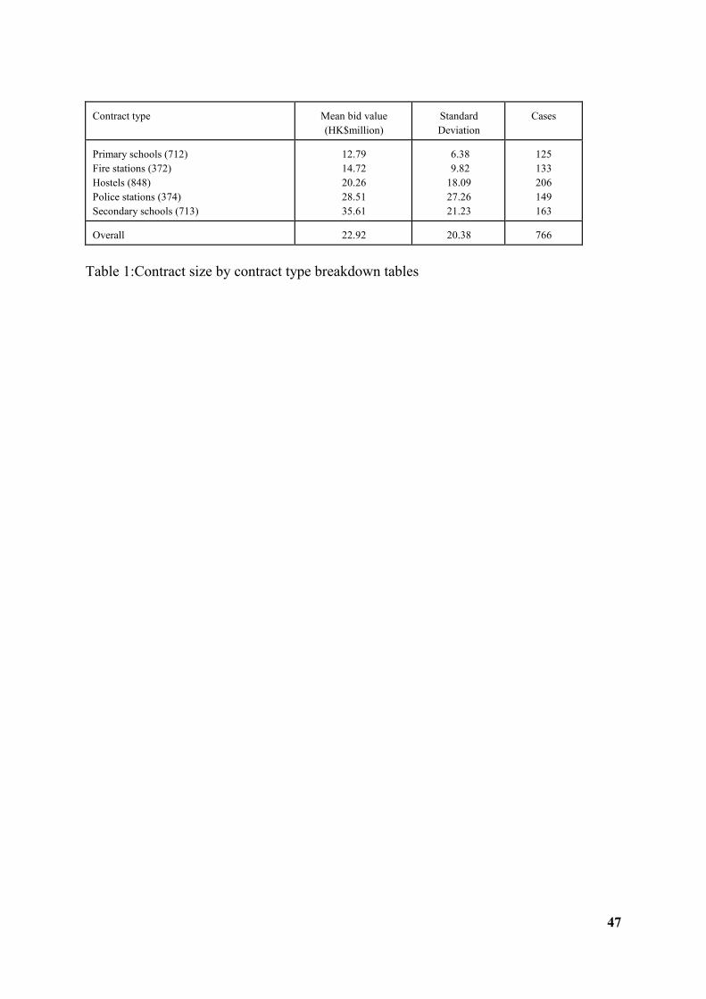
47

Contract type Mean bid value

(HK$million)

Standard

Deviation

Cases

Primary schools (712)

Fire stations (372)

Hostels (848)

Police stations (374)

Secondary schools (713)

12.79

14.72

20.26

28.51

35.61

6.38

9.82

18.09

27.26

21.23

125

133

206

149

163

Overall 22.92 20.38 766

Table 1:Contract size by contract type breakdown tables

48

15 BIDDERS 5 TYPES

Model No.

Explained df

Residual df

SSE M S Error

F Value

Adjusted R2

1 2 3 5 4 7 8 6 9 12 10 13 14 21 11 15 16 18 17 20 19 22

0 3 7 15 17 21 29 45 49 57 77 85 105 113 133 141 161 169 189 197 217 225

776 773 769 761 759 755 747 731 727 719 699 691 671 663 643 635 615 607 587 579 559 551

8.38 8.01 7.79 7.53 6.80 6.64 6.39 6.20 6.06 5.80 6.03 5.83 5.50 5.29 5.67 5.30 5.13 4.78 4.73 4.63 4.52 4.43

0.010799 0.010362 0.010130 0.009895 0.008959 0.008795 0.008554 0.008482 0.008336 0.008067 0.008627 0.008437 0.008197 0.007979 0.008818 0.008346 0.008341 0.007875 0.008058 0.007997 0.008086 0.008040

0.00 17.85 9.71 6.14 11.02 9.89 8.31 5.84 5.80 5.71 3.58 3.60 3.38 3.46 2.33 2.64 2.44 2.72 2.41 2.39 2.21 2.19

0.00 0.04 0.06 0.08 0.17 0.19 0.21 0.21 0.23 0.25 0.20 0.22 0.24 0.26 0.18 0.23 0.23 0.27 0.25 0.26 0.25 0.26

Table 2:Summary of candidate model statistics

49

15 BIDDERS 5 TYPES

Compared Models

Calculated Value

Tabulated Value

Accepted Model No.

1 / 2 2 / 3 3 / 5 5 / 4 4 / 7 7 / 8 8 / 6 8 / 9 9 / 12 12 / 10 12 / 13 12 / 14 12 / 21 12 / 11 12 / 15 12 / 16 12 / 18 12 / 17 12 / 20 12 / 19 12 / 22

11.90 5.43 3.28 40.74 4.55 3.65 1.40 1.98 4.03 - - 0.76 1.14 0.19 0.71 0.77 1.16 1.01 1.05 0.99 1.01

2.61 2.38 1.95 3.01 2.38 1.96 1.48 1.59 1.96 1.59 1.48 1.37 1.35 1.31 1.29 1.27 1.26 1.25 1.24 1.23 1.23

2 3 5 4 7 8 8 9 12 12 12 12 12 12 12 12 12 12 12 12 12

Table 3:Summary of candidate model calculated and tabulated F values