cpet-it user's manual v.1 - geologismikigeologismiki.gr/documents/cpet-it/cpet-it...
TRANSCRIPT
© 2014 GeoLogismiki
CPeT-IT User's Manual v.1.4

All rights reserved. No parts of this work may be reproduced in any form or by any means - graphic, electronic, ormechanical, including photocopying, recording, taping, or information storage and retrieval systems - without thewritten permission of the publisher.
Products that are referred to in this document may be either trademarks and/or registered trademarks of therespective owners. The publisher and the author make no claim to these trademarks.
While every precaution has been taken in the preparation of this document, the publisher and the author assume noresponsibility for errors or omissions, or for damages resulting from the use of information contained in thisdocument or from the use of programs and source code that may accompany it. In no event shall the publisher andthe author be liable for any loss of profit or any other commercial damage caused or alleged to have been causeddirectly or indirectly by this document.
Printed: Σεπτέµβριος 2014
CPeT-IT User's Manual v.1.4
© 2014 GeoLogismiki
3Contents
© 2014 GeoLogismiki
Table of Contents
Foreword 0
Part I License Agreement 5
Part II Introduction 6
Part III Overview 7
................................................................................................................................... 91 Starting a new project
................................................................................................................................... 102 Importing CPTU data
......................................................................................................................................................... 14Importing .cor files
......................................................................................................................................................... 15Importing .xls files
......................................................................................................................................................... 16Importing .gef files
................................................................................................................................... 193 Defining CPT parameters
......................................................................................................................................................... 23Transition layer detection
................................................................................................................................... 244 Editing CPT data
......................................................................................................................................................... 28Direct edit raw CPT data
................................................................................................................................... 285 Loading a project
................................................................................................................................... 296 Saving a project
................................................................................................................................... 307 Printing results
Part IV Advanced features 33
................................................................................................................................... 331 Importing data from other applications
................................................................................................................................... 352 Adding sample data
................................................................................................................................... 373 Adding custom estimations data
................................................................................................................................... 384 Customizing Reports
......................................................................................................................................................... 40Custom Report Page
......................................................................................................................................................... 42Terms & Conditions
................................................................................................................................... 435 Creating overlay report
................................................................................................................................... 466 Working with plots
......................................................................................................................................................... 46Customizing plots
......................................................................................................................................................... 50Exporting plots
......................................................................................................................................................... 53Navigation helper tool
................................................................................................................................... 537 Filtering CPT Data
......................................................................................................................................................... 54Cross Correlate
......................................................................................................................................................... 55Spike Filter
......................................................................................................................................................... 57Shift Raw Data
......................................................................................................................................................... 58Depth Correction
......................................................................................................................................................... 59Negative Values Filter
......................................................................................................................................................... 59Pore Pressure Converter
................................................................................................................................... 608 Single pile bearing capacity
................................................................................................................................... 659 Dissipation test interpretation
......................................................................................................................................................... 68Importing dissipation test data
CPeT-IT User's Manual v.1.44
© 2014 GeoLogismiki
................................................................................................................................... 7010 Settlements calculation
................................................................................................................................... 7411 Geotechnical section creation
......................................................................................................................................................... 80Semi auto soil layer boundaries detection
......................................................................................................................................................... 82Geotechnical section layers statistics
................................................................................................................................... 8512 Exporting data
......................................................................................................................................................... 85Exporting results to XLS file
......................................................................................................................................................... 86Exporting data for LiqIT
Part V Note 86
Part VI LCPC method 89
Part VII References 92
Index 0
5License Agreement
© 2014 GeoLogismiki
1 License AgreementCPeT-IT EULA
END-USER LICENSE AGREEMENT FOR CPeT-IT IMPORTANT PLEASE READ THE TERMSAND CONDITIONS OF THIS LICENSE AGREEMENT CAREFULLY BEFORE CONTINUINGWITH THIS PROGRAM INSTALL: GeoLogismiki End-User License Agreement ("EULA") is alegal agreement between you (either an individual or a single entity) and GeoLogismiki.for the GeoLogismiki software identified above which may include associated softwarecomponents, media, printed materials, and "online" or electronic documentation("CPeT-IT"). By installing, copying, or otherwise using the CPeT-IT, you agree to bebound by the terms of this EULA. This license agreement represents the entireagreement concerning the program between you and GeoLogismiki, (referred to as"licenser"), and it supersedes any prior proposal, representation, or understandingbetween the parties. If you do not agree to the terms of this EULA, do not install oruse CPeT-IT. CPeT-IT is protected by copyright laws and international copyright treaties, as well asother intellectual property laws and treaties. CPeT-IT is licensed, not sold.
GRANT OF LICENSE.
CPeT-IT is licensed as follows:(a) Installation and Use.GeoLogismiki grants you the right to install and use copies of CPeT-IT on yourcomputer running a validly licensed copy of the operating system for which CPeT-ITwas designed [Windows 2000, Windows XP].(b) Backup Copies.You may also make copies of CPeT-IT as may be necessary for backup and archivalpurposes.
DESCRIPTION OF OTHER RIGHTS AND LIMITATIONS.
(a) Maintenance of Copyright Notices.You must not remove or alter any copyright notices on any and all copies of CPeT-IT.(b) Distribution.You may not distribute registered copies of CPeT-IT to third parties. Evaluationversions available for download from GeoLogismiki’s websites may be freely distributed.(c) Prohibition on Reverse Engineering, Decompilation, and Disassembly.You may not reverse engineer, decompile, or disassemble CPeT-IT, except and only tothe extent that such activity is expressly permitted by applicable law notwithstandingthis limitation. (d) Rental.You may not rent, lease, or lend CPeT-IT.(e) Support Services.GeoLogismiki may provide you with support services related to CPeT-IT ("SupportServices"). Any supplemental software code provided to you as part of the SupportServices shall be considered part of the CPeT-IT and subject to the terms andconditions of this EULA.(f) Compliance with Applicable Laws.You must comply with all applicable laws regarding use of CPeT-IT.
TERMINATION
Without prejudice to any other rights, GeoLogismiki may terminate this EULA if you failto comply with the terms and conditions of this EULA. In such event, you must destroy
6 CPeT-IT User's Manual v.1.4
© 2014 GeoLogismiki
all copies of CPeT-IT in your possession.
COPYRIGHT
All title, including but not limited to copyrights, in and to CPeT-IT and any copiesthereof are owned by GeoLogismiki. All title and intellectual property rights in and tothe content which may be accessed through use of CPeT-IT is the property of therespective content owner and may be protected by applicable copyright or otherintellectual property laws and treaties. This EULA grants you no rights to use suchcontent. All rights not expressly granted are reserved by GeoLogismiki.
NO WARRANTIES
GeoLogismiki expressly disclaims any warranty for CPeT-IT. CPeT-IT is provided “As Is”without any express or implied warranty of any kind, including but not limited to anywarranties of merchantability, noninfringement, or fitness of a particular purpose.GeoLogismiki does not warrant or assume responsibility for the accuracy orcompleteness of any information, calculation, text, graphics, links or other itemscontained within CPeT-IT. GeoLogismiki makes no warranties respecting any harm thatmay be caused by the transmission of a computer virus, worm, time bomb, logic bomb,or other such computer program. GeoLogismiki further expressly disclaims any warrantyor representation to Authorized Users or to any third party.
LIMITATION OF LIABILITY
In no event shall GeoLogismiki be liable for any damages (including, without limitation,lost profits, business interruption, or lost information) rising out of Authorized Users'use of or inability to use CPeT-IT, even if GeoLogismiki has been advised of thepossibility of such damages. In no event will GeoLogismiki be liable for loss of data orfor indirect, special, incidental, consequential (including lost profit), or other damagesbased in contract, tort or otherwise. GeoLogismiki shall have no liability with respect tothe content of the CPeT-IT or any part thereof, including but not limited to errors oromissions contained therein, libel, infringements of rights of publicity, privacy,trademark rights, business interruption, personal injury, loss of privacy, moral rights orthe disclosure of confidential information.
OTHER RIGHTS AND RESTRICTIONS
All other rights and restrictions not specifically granted in this license are reserved byus. If you have any questions regarding this agreement, please write [email protected]
YOU ACKNOWLEDGE THAT YOU HAVE READ THIS AGREEMENT, UNDERSTAND IT ANDAGREE TO BE BOUND BY ITS TERMS AND CONDITIONS.
2 Introduction
CPeT-IT is software for interpretation of CPTU data. CPeT-IT was developed incollaboration with Gregg Drilling & Testing Inc., a leading company in site investigationand CPT, and Professor Peter Robertson, co-author of the comprehensive text book onthe CPT.
CPeT-IT takes CPT data and performs basic interpretation in terms of Soil BehaviourType (SBT) and various geotechnical soil and design parameters using current
7Introduction
© 2014 GeoLogismiki
published correlations based on the comprehensive review by Lunne, Robertson andPowell (1997), as well as recent updates by Professor Robertson. The interpretationsare presented only as a guide for geotechnical use and should be carefully reviewed.Either GeoLogismiki or Gregg Drilling Inc., does not warranty the correctness or theapplicability of any of the geotechnical soil and design parameters interpreted by thesoftware and does not assume any liability for any use of the results in any design orreview. The user should be fully aware of the techniques and limitations of any methodused in the software.
3 Overview
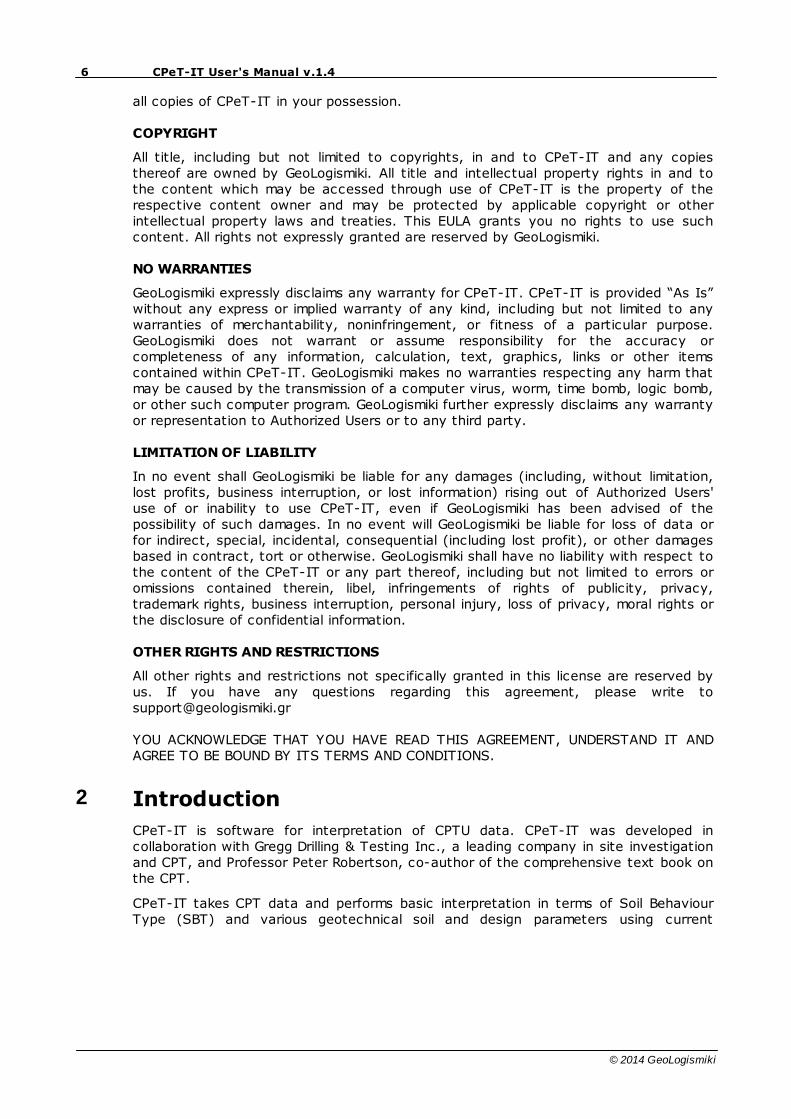
The software's main window is divided into two areas. In the left area, under the titleCPT file manager, it displays a list with the available CPTU data and in the large rightarea CPeT-IT will display input and output results in both tabular and graphic format.This way you can always have an instant preview of your data and estimations forquick reference.
CPeT-IT application window
The right hand side of the main window shows tabular output in the top half and plotsin the lower half. The top half has two tabs, one for Basic Results and the other forEstimated Parameters. The relative size of the top and lower windows can be adjustedby clicking and dragging the horizontal dividing bar.
8 CPeT-IT User's Manual v.1.4
© 2014 GeoLogismiki
When the Basic Results tab is activated, the table shows the measured CPT input dataand basic output data as a function of depth. The lower half shows the various BasicResults - Data Plots.
Data plots
At the base of the main window, the Raw data plots are displayed along with tabs toshow, Basic plots, Normalized plots and SBT plots.
Raw data plots: This window displays plots of measured, cone tip resistance, qc,
sleeve friction, fs, and penetration pore pressure, u, and cross correlation between q
c
and fs. A hydrostatic pore pressure line is also shown on the CPT pore pressure plot to
act as reference and is determined based on the user input of ground water level(GWL). The cross correlation plot is a comparison between the q
c and f
s profiles. Since
the center of the friction sleeve is physically several centimeters behind the cone tip(actual distance will depend on cone size, e.g. 10 cm² or 15 cm²), most contractorsoffset the data so that both the tip, friction and pore pressure are shown at the samedepth, rather than the same time. The cross correlation plot provides a check toevaluate if the offset has been fully effective or to determine if the data set has notbeen corrected for the physical offset. If the data has been fully offset, the crosscorrelation should show a maximum values at zero offset. In highly interbedded profiles,the cross correlation may not always show a clear maximum value.
Basic Plots: This window displays plots of corrected, qt, friction ratio, R
f, penetration
pore pressure, u (with reference hydrostatic profile based on user input GWL),normalized SBT
n I
c, and non-normalized SBT.
Normalized Plots: This window displays plots of normalized CPT parameters,normalized tip resistance, Q
tn, normalized friction ratio, F
r, normalized pore pressure
parameter, Bq, normalized SBT
n I
c and normalized SBT
n.
SBT plots: This window displays the CPT results on both the non-normalized andnormalized CPT Soil Behaviour Type (SBT and SBT
n) charts suggested by Robertson et
al., 1986, and Robertson, 1990. When the cursor (with "SHIFT" key pressed) is movedover the CPT data, the depth of the data point is displayed and the associated line ofdata are highlighted in the table above.
Bq plots: This window displays the CPTu results on both the non-normalized andnormalized CPT Soil Behavior Type charts based on normalized pore pressureparameter, Bq.
Schneider Plots: This window displays soil classification plots suggested by JamesSchneider et al. based on normalized excess pore pressure.
When the Estimated Parameters tab is activated, the table shows the calculatedgeotechnical parameters based on the user input constants. The lower half showsplots of estimated parameters versus depth under three tabs, Estimated Plots 1,Estimated Plots 2 and Estimated Plots 3.
As with all plots the scales can be adjusted (see Customizing plots).
9Overview
© 2014 GeoLogismiki
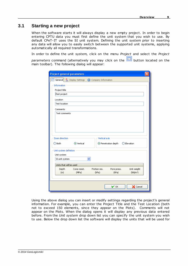
3.1 Starting a new project
When the software starts it will always display a new empty project. In order to beginentering CPTU data you must first define the unit system that you wish to use. Bydefault CPeT-IT uses the SI unit system. Defining the unit system prior to insertingany data will allow you to easily switch between the supported unit systems, applyingautomatically all required transformations.
In order to define the unit system, click on the menu Project and select the Project
parameters command (alternatively you may click on the button located on themain toolbar). The following dialog will appear:
Using the above dialog you can insert or modify settings regarding the project's generalinformation. For example, you can enter the Project Title and the Test Location (bothnot to exceed 150 elements, since they appear on the Plots). Comments will notappear on the Plots. When the dialog opens it will display any previous data enteredbefore. From the Unit system drop down list you can specify the unit system you wishto use. Below the drop down list the software will display the units that will be used for
10 CPeT-IT User's Manual v.1.4
© 2014 GeoLogismiki
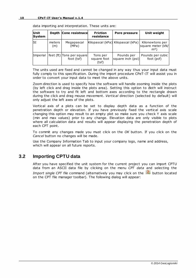
data importing and interpretation. These units are:
UnitSystem
Depth Cone resistnace Frictionresistance
Pore pressure Unit weight
SI meters(m)
Megapascal(MPa)
Kilopascal (kPa) Kilopascal (kPa) Kilonewtons persquare meter (kN/
m³)
Imperial feet (ft) Tons per squarefoot (tsf)
Tons persquare foot
(tsf)
Pounds persquare inch (psi)
Pounds per cubicfoot (pcf)
The units used are fixed and cannot be changed in any way thus your input data mustfully comply to this specification. During the import procedure CPeT-IT will assist you inorder to convert your input data to meet the above units.
Zoom direction is used to specify how the software will handle zooming inside the plots(by left click and drag inside the plots area). Setting this option to Both will instructthe software to try and fit left and bottom axes according to the rectangle drawnduring the click and drag mouse movement. Vertical direction (selected by default) willonly adjust the left axes of the plots.
Vertical axis of a plots can be set to display depth data as a function of thepenetration depth or elevation. If you have previously fixed the vertical axis scalechanging this option may result to an empty plot so make sure you check Y axis scale(min and max values) prior to any change. Elevation data are only visible to plotswhere all calculation data and results will appear displaying the penetration depth ofeach CPT point.
To commit any changes made you must click on the OK button. If you click on theCancel button no changes will be made.
Use the Company Information Tab to input your company logo, name and address,which will appear on all future reports.
3.2 Importing CPTU data
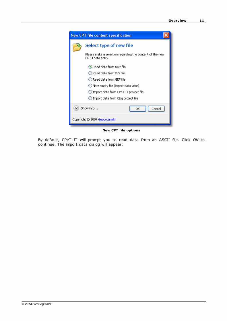
After you have specified the unit system for the current project you can import CPTUdata from an ASCII data file by clicking on the menu CPT data and selecting the
Import single CPT file command (alternatively you may click on the button locatedon the CPT file manager toolbar). The following dialog will appear:
11Overview
© 2014 GeoLogismiki
New CPT file options
By default, CPeT-IT will prompt you to read data from an ASCII file. Click OK tocontinue. The import data dialog will appear:
12 CPeT-IT User's Manual v.1.4
© 2014 GeoLogismiki
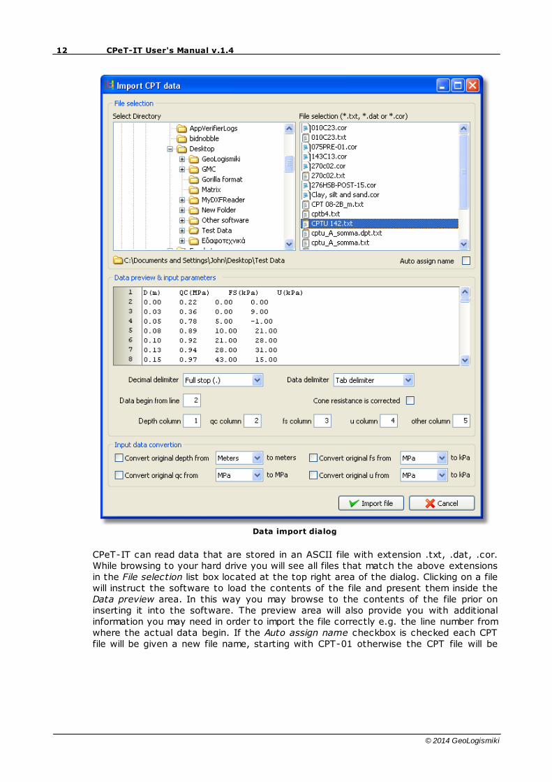
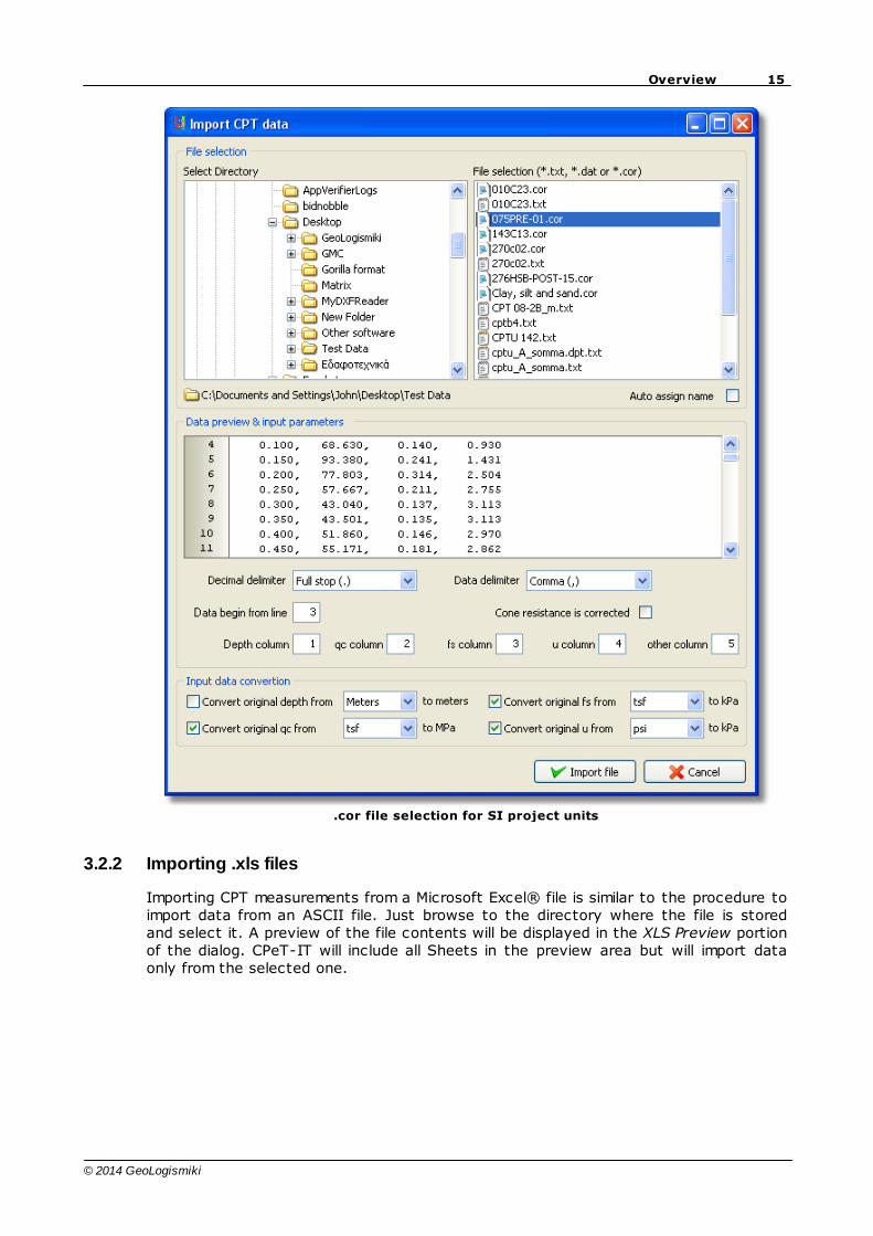
Data import dialog
CPeT-IT can read data that are stored in an ASCII file with extension .txt, .dat, .cor.While browsing to your hard drive you will see all files that match the above extensionsin the File selection list box located at the top right area of the dialog. Clicking on a filewill instruct the software to load the contents of the file and present them inside theData preview area. In this way you may browse to the contents of the file prior oninserting it into the software. The preview area will also provide you with additionalinformation you may need in order to import the file correctly e.g. the line number fromwhere the actual data begin. If the Auto assign name checkbox is checked each CPTfile will be given a new file name, starting with CPT-01 otherwise the CPT file will be
13Overview
© 2014 GeoLogismiki
named after the associated file name without the file extension (e.g. .cor). The filename can be changed to match the actual file name by using the CPT data – RenameCPT feature when a file is highlighted. You may also select multiple files by holdingdown the Ctrl key on the keyboard while clicking on the file names.
As a general rule, the data file must contain at least 4 columns of data in the followingorder, depth - cone resistance - friction resistance - pore pressure (where porepressure is the penetration pore pressure u measured behind the cone e.g. u2).Additionally the program will look for a fifth column which may contain any other datasuch as electrical resistivity or UVIF. If other columns exist in the data file thesoftware will ignore them.
Based on the data preview, you must provide the software with additional informationregarding the data structure inside the file. CPeT-IT needs to know what character isused as a decimal delimiter, what character is used as a data delimiter (separationcharacter between column data), from which line the actual data start (after anyheader information) and if the data file contains the raw cone resistancemeasurements (there are cases where your CPT contractor may give you a filecontaining the corrected cone penetration resistance q
t instead of the raw field value
qc). Making the right selections inside the Data input parameters is very crucial for a
successive completion of the import procedure.
Finally, in case that the data in your file do not meet the units specification you canselect the corresponding check box for the value you wish to convert e.g. if your datafile contains depth measurements in feet and your project's unit system is set to SIthen you should check the Convert original depth from checkbox and from the dropdown list select feet.
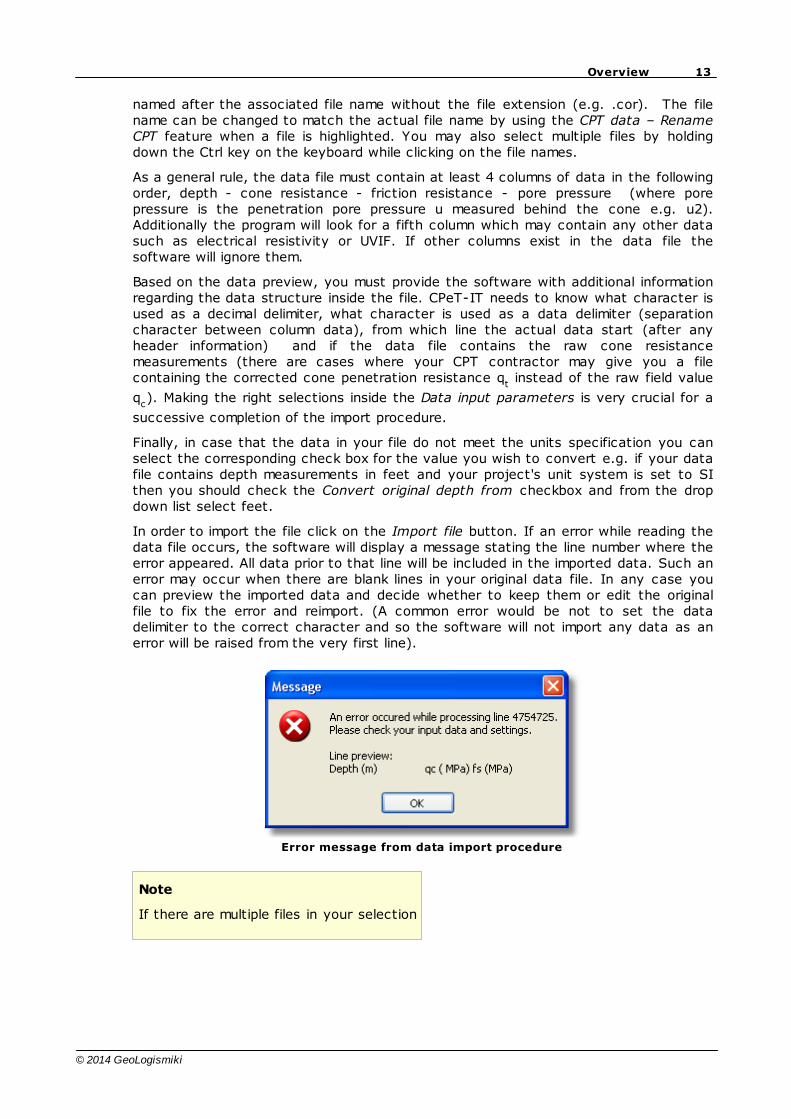
In order to import the file click on the Import file button. If an error while reading thedata file occurs, the software will display a message stating the line number where theerror appeared. All data prior to that line will be included in the imported data. Such anerror may occur when there are blank lines in your original data file. In any case youcan preview the imported data and decide whether to keep them or edit the originalfile to fix the error and reimport. (A common error would be not to set the datadelimiter to the correct character and so the software will not import any data as anerror will be raised from the very first line).
Error message from data import procedure
Note
If there are multiple files in your selection

14 CPeT-IT User's Manual v.1.4
© 2014 GeoLogismiki
you must make sure that the filestructure is common to all selected filesotherwise the import procedure will fail toread all files
3.2.1 Importing .cor files
Gregg Drilling Inc., provides its customers with an ASCII text file containing the rawCPTU field measurements. This file has an extension .cor and when selected thesoftware will make the appropriate adjustments for the various data input parametersand convertions automatically. After selecting such a file just click on the Importbutton to let the software read and import the data to your new CPT entry.
15Overview
© 2014 GeoLogismiki
.cor file selection for SI project units
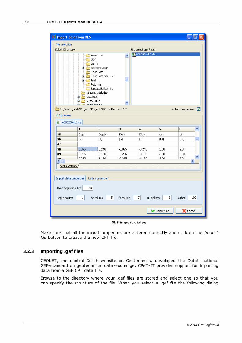
3.2.2 Importing .xls files
Importing CPT measurements from a Microsoft Excel® file is similar to the procedure toimport data from an ASCII file. Just browse to the directory where the file is storedand select it. A preview of the file contents will be displayed in the XLS Preview portionof the dialog. CPeT-IT will include all Sheets in the preview area but will import dataonly from the selected one.
16 CPeT-IT User's Manual v.1.4
© 2014 GeoLogismiki
XLS import dialog
Make sure that all the import properties are entered correctly and click on the Importfile button to create the new CPT file.
3.2.3 Importing .gef files
GEONET, the central Dutch website on Geotechnics, developed the Dutch nationalGEF-standard on geotechnical data-exchange. CPeT-IT provides support for importingdata from a GEF CPT data file.
Browse to the directory where your .gef files are stored and select one so that youcan specify the structure of the file. When you select a .gef file the following dialog
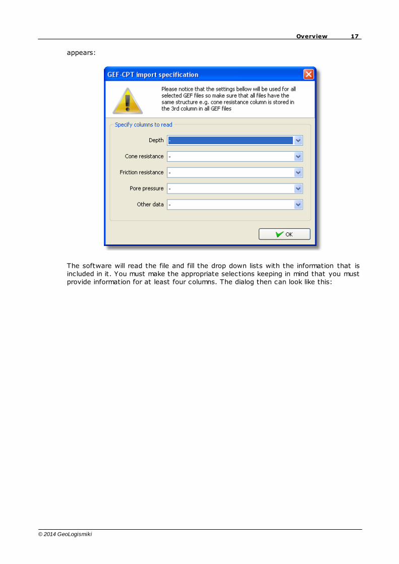
17Overview
© 2014 GeoLogismiki
appears:
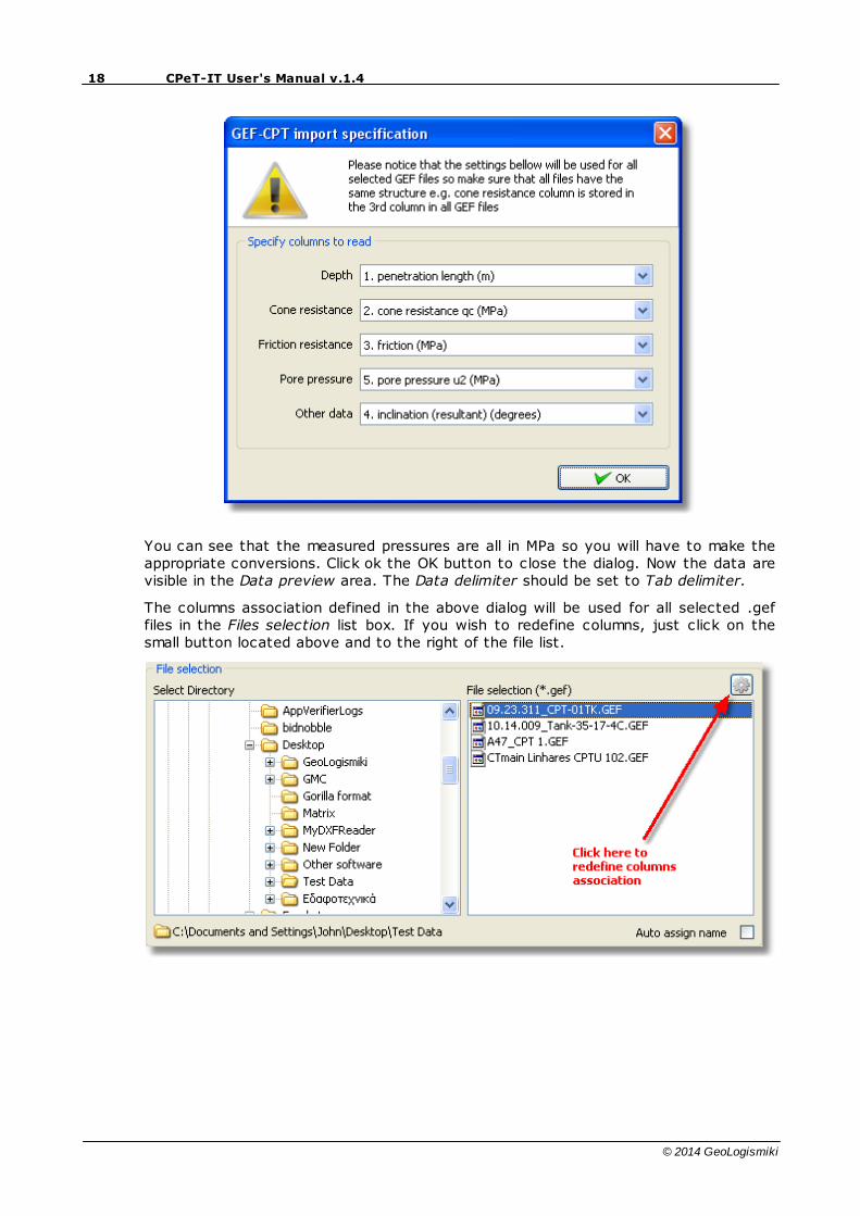
The software will read the file and fill the drop down lists with the information that isincluded in it. You must make the appropriate selections keeping in mind that you mustprovide information for at least four columns. The dialog then can look like this:
18 CPeT-IT User's Manual v.1.4
© 2014 GeoLogismiki
You can see that the measured pressures are all in MPa so you will have to make theappropriate conversions. Click ok the OK button to close the dialog. Now the data arevisible in the Data preview area. The Data delimiter should be set to Tab delimiter.
The columns association defined in the above dialog will be used for all selected .geffiles in the Files selection list box. If you wish to redefine columns, just click on thesmall button located above and to the right of the file list.
19Overview
© 2014 GeoLogismiki
3.3 Defining CPT parameters
CPeT-IT uses established empirical correlations to estimate geotechnical parameters.Many of them have constants that have a range of values depending on soil type,geologic origin and other factors. The software uses default values that have beenselected to provide, in general, conservatively low estimates of the variousgeotechnical parameters. These default values are assigned to every new CPTU datayou import automatically.
The following empirical correlations have been used to calculate parameters:
Input:
Units for display (Imperial or metric) (atm. pressure, pa = 0.96 tsf or 0.1MPa)
Elevation of ground surface (ft or m)
Depth to water table, zw (ft or m) – input required for each CPT sounding.
Equilibrium water pressures are assumed hydrostatic relative to the inputGWL
Net area ratio for cone, a (default to 0.80)
Relative Density constant, CDr (default to 350)
Undrained shear strength cone factor for clays, Nkt (default to 14)
Over Consolidation ratio number, kocr (default to 0.33)
Unit weight of water, (default to gw = 62.4 lb/ft³ or 9.81 kN/m³)
Probe radius (default to 0.0183 m)
Output:
Total cone resistance, qt (tsf or MPa) qt = qc + u x (1-a)
Friction Ratio, Rf (%) Rf = (fs/qt) x 100%
Soil Behavior Type (non-normalized), SBT see note
Unit weight, g (pcf or kN/m³) based on SBT, see note
Total overburden stress, sv (tsf) svo = g x z
Insitu pore pressure, uo (tsf) uo = gw x (z - zw)
Effective overburden stress, s'vo (tsf ) s'vo = svo - uo
Normalized cone resistance, Qt1 Qt1 = (qt - svo) / s'vo
Normalized friction ratio, Fr (%) Fr = fs / (qt - svo) x 100%
Normalized Pore Pressure ratio, Bq Bq = u – uo / (qt - svo)
Soil Behavior Type (normalized), SBTn see note
20 CPeT-IT User's Manual v.1.4
© 2014 GeoLogismiki
SBTn Index, Ic see note
Normalized Cone resistance, Qtn (n varies with Ic) see note
Estimated permeability, kSBT (cm/sec or ft/sec) see note
Equivalent SPT N60, (blows/ft or blows/30cm) see note
Estimated Constrained Modulus, M see note
Estimated Relative Density, Dr, (%) see note
Estimated Friction Angle, f', (degrees) see note
Estimated Young’s modulus, Es (tsf or MPa) see note
Estimated small strain Shear modulus, Go (tsf or MPa) see note
Estimated Undrained shear strength, su (tsf or kPa) see note
Estimated Undrained strength ratio su/sv'
Estimated Over Consolidation ratio, OCR see note
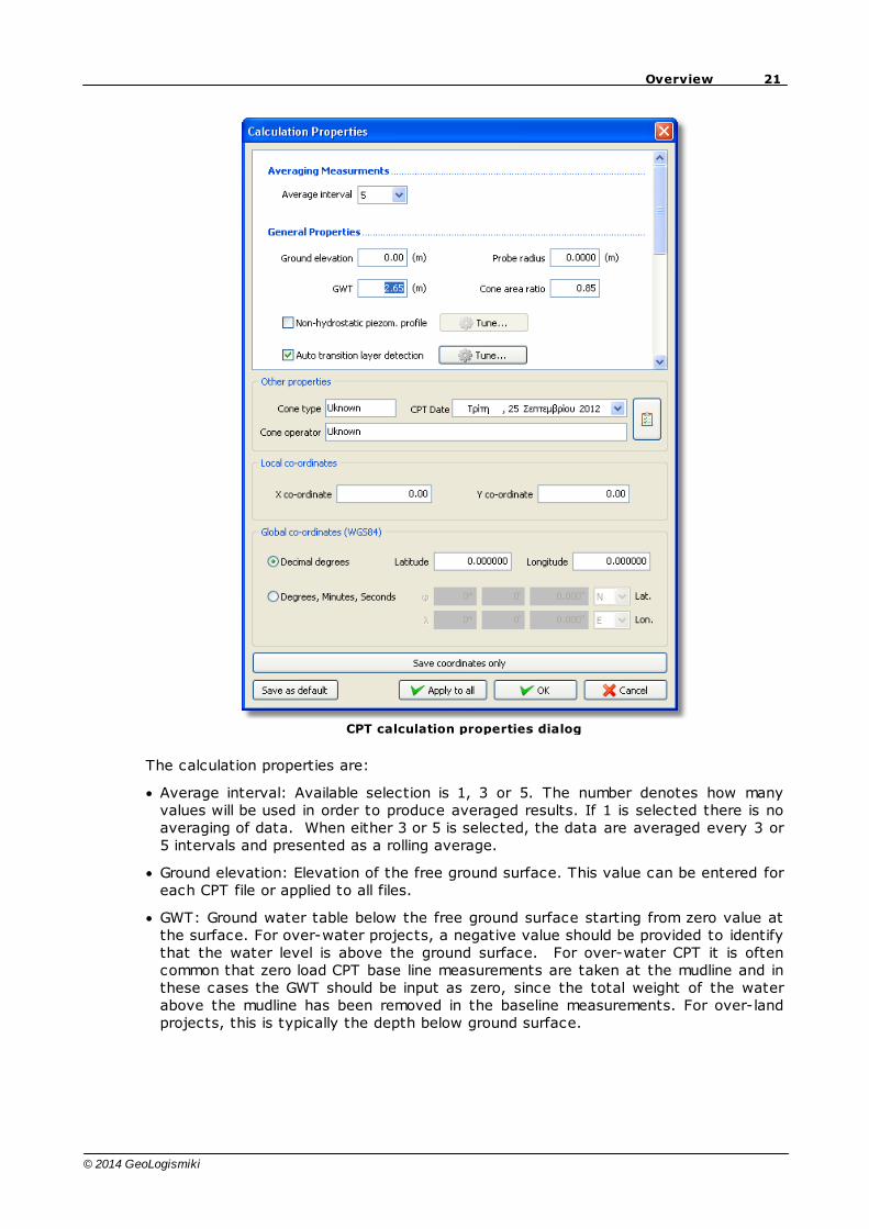
In order to view or edit these constants select a CPTU sounding and from the menu
CPT data click on the CPT Properties command (alternatively you may click on the button located on the CPT File Manger toolbar). The following dialog will appear:
21Overview
© 2014 GeoLogismiki
CPT calculation properties dialog
The calculation properties are:
Average interval: Available selection is 1, 3 or 5. The number denotes how manyvalues will be used in order to produce averaged results. If 1 is selected there is noaveraging of data. When either 3 or 5 is selected, the data are averaged every 3 or5 intervals and presented as a rolling average.
Ground elevation: Elevation of the free ground surface. This value can be entered foreach CPT file or applied to all files.
GWT: Ground water table below the free ground surface starting from zero value atthe surface. For over-water projects, a negative value should be provided to identifythat the water level is above the ground surface. For over-water CPT it is oftencommon that zero load CPT base line measurements are taken at the mudline and inthese cases the GWT should be input as zero, since the total weight of the waterabove the mudline has been removed in the baseline measurements. For over-landprojects, this is typically the depth below ground surface.
22 CPeT-IT User's Manual v.1.4
© 2014 GeoLogismiki
Probe radius: Radius of the cone used for the calculation of ch in the dissipation
module.
Cone area ratio: The net area ratio for the cone (default value to 0.85).
Non-hydrostatic piezom. profile: When checked a custom profile of pore pressurevalues may be defined and used.
Cone resistance is corrected: When checked the software will assume that importedraw cone resistance q
c is already corrected and equal to q
t
Unit weight of water: Unit weight of water (default value to 9.81 kN/m³ or 62.40 lb/ft³).
Auto unit weight: When checked the software will use a built-in function to estimateunit weight based on q
t and R
f. If unchecked then a list of custom values can be
used or apply the constant value entered in the edit box.
Auto OCR number: When checked the software will try to estimate over consolidationratio number, k
ocr for every CPT point. If unchecked then a custom constant value is
used (default value to 0.33).
Auto Nkt
: If checked then undrained shear strength cone factor for clays, Nkt
will be
estimated by the software at every CPT point otherwise a constant value will beapplied (default value to 14).
Dr constant: Relative density constant, C
Dr (default value to 350).
Cn
cutoff: At very low penetration depths (close to the free ground surface)
normalization factor n may take large values resulting to large Qtn
values. Enabling
this option will set a maximum to the calculate Cn (default value is 2.00)
Ns: This is a constant used for the calculation of soil sensitivity (ranges between 5.0
to 10.0 with an average value of 7.10)
Calculate SPT: Selection to choose between the estimation of corrected N60
SPT
values or normalized corrected SPT values N1(60)
Auto transition layer detection: When checked the software will try to detect datathat are in transition from either clay to sand or vise-versa. Data belonging totransition zones will not be plotted in the estimations plots and will not contribute toaverage values used in the Geotechnical Section module. Click on the Tune buttonto fine tune the detection algorithm.
In order to apply any changes made to the selected CPTU just click on the OK button.If you wish the changes made to be the default values for every CPTU that you willcreate click on the Save as default button. If you click on the Apply to all button, allvalues entered in this dialog will be applied to every CPTU sounding in the currentproject. Save coordinates only button will cause the dialog to close applying thechanges made to coordinates only.
Closing the above dialog will not cause any recalculation of the estimated properties.To do so you will either need to recalculate all CPTU soundings or just the selectedone. Click on the Calculation menu and select the appropriate command. Alternatively
23Overview
© 2014 GeoLogismiki
you may click on the button in order to recalculate all CPTU soundings.
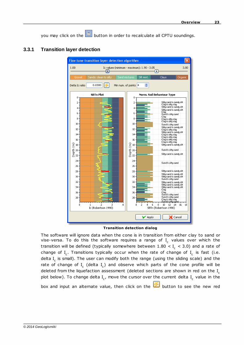
3.3.1 Transition layer detection
Transition detection dialog
The software will ignore data when the cone is in transition from either clay to sand orvise-versa. To do this the software requires a range of I
c values over which the
transition will be defined (typically somewhere between 1.80 < Ic < 3.0) and a rate of
change of Ic. Transitions typically occur when the rate of change of I
c is fast (i.e.
delta Ic is small). The user can modify both the range (using the sliding scale) and the
rate of change of Ic (delta I
c) and observe which parts of the cone profile will be
deleted from the liquefaction assessment (deleted sections are shown in red on the Ic
plot below). To change delta Ic, move the cursor over the current delta I
c value in the
box and input an alternate value, then click on the button to see the new red
24 CPeT-IT User's Manual v.1.4
© 2014 GeoLogismiki
sections that will be deleted. The user can also move the sliding scales above tomodify the range of I
c to define the transition. User judgment is required to optimize
the amount of data that will be deleted. Finally, using the Min num. of points edit boxyou may instruct the software to keep detected transition layers with a minimumnumber of CPT points according to the number entered. Using the up and down arrowsCPeT-IT will recalculate the layers automatically.
Click on the Apply button to accept changes made.
3.4 Editing CPT data
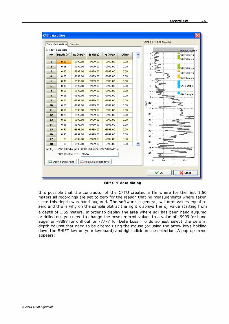
It is a common practice to hand auger the first centimeters before inserting the coneto the ground. Also, during the test, the cone can meet refusal on a soil layer thatcannot penetrate and special treatment should be made, allowing the cone to continueafter the hard layer has been drilled out. To include such information in your CPTU dataand be able to present it in the raw input plots, select a CPTU element and from themenu CPT data click on the Edit CPT data command. The following dialog will appear:
25Overview
© 2014 GeoLogismiki
Edit CPT data dialog
It is possible that the contractor of the CPTU created a file where for the first 1.50meters all recordings are set to zero for the reason that no measurements where takensince this depth was hand augured. The software in general, will omit values equal tozero and this is why on the sample plot at the right displays the q
c value starting from
a depth of 1.55 meters. In order to display the area where soil has been hand auguredor drilled out you need to change the measurement values to a value of -9999 for handauger or -8888 for drill out or -7777 for Data Loss. To do so just select the cells indepth column that need to be altered using the mouse (or using the arrow keys holdingdown the SHIFT key on your keyboard) and right click on the selection. A pop up menuappears:
26 CPeT-IT User's Manual v.1.4
© 2014 GeoLogismiki
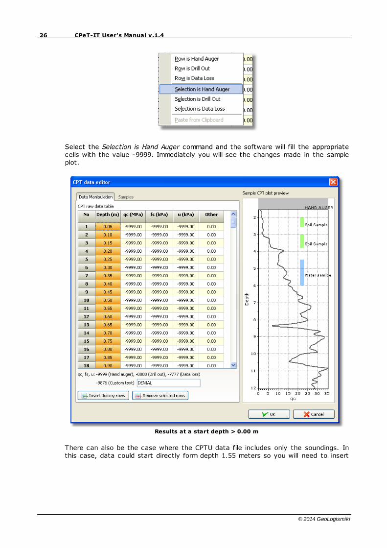
Select the Selection is Hand Auger command and the software will fill the appropriatecells with the value -9999. Immediately you will see the changes made in the sampleplot.
Results at a start depth > 0.00 m
There can also be the case where the CPTU data file includes only the soundings. Inthis case, data could start directly form depth 1.55 meters so you will need to insert
27Overview
© 2014 GeoLogismiki
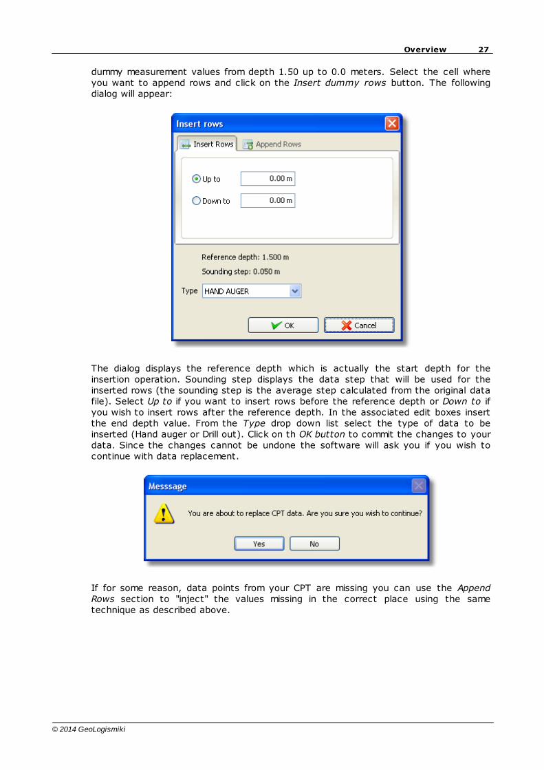
dummy measurement values from depth 1.50 up to 0.0 meters. Select the cell whereyou want to append rows and click on the Insert dummy rows button. The followingdialog will appear:
The dialog displays the reference depth which is actually the start depth for theinsertion operation. Sounding step displays the data step that will be used for theinserted rows (the sounding step is the average step calculated from the original datafile). Select Up to if you want to insert rows before the reference depth or Down to ifyou wish to insert rows after the reference depth. In the associated edit boxes insertthe end depth value. From the Type drop down list select the type of data to beinserted (Hand auger or Drill out). Click on th OK button to commit the changes to yourdata. Since the changes cannot be undone the software will ask you if you wish tocontinue with data replacement.
If for some reason, data points from your CPT are missing you can use the AppendRows section to "inject" the values missing in the correct place using the sametechnique as described above.
28 CPeT-IT User's Manual v.1.4
© 2014 GeoLogismiki
3.4.1 Direct edit raw CPT data
Sometimes it may be useful to edit a few raw measurements in order for example to fixpeaks in qc profile due to rod change. The software provides a quick and easy way tolocate and fix these values without the use of the CPT data editor. The procedure isdescribed below:
1. Enable the direct edit mode by clicking on the button on the main toolbar orfrom the CPT Data menu select the Enable Direct Edit Raw Data command. The icon on
the toolbar will remain pressed (highlighted) to visually inform that the feature isenabled.
2. By holding the SHIFT key on your keyboard locate the value you wish to fix.
3. Click on the corresponding cell and edit the value. Press Enter on your keyboard tocommit the change or just click anywhere outside the cell. The plot will be updatedautomatically but no calculations are performed during this step.
4. Disable the feature by clicking on the highlighted icon (in order to avoid anyaccidental changes in raw data) and recalculate your CPT.
Note
Direct edit mode allowschanges to depth, q
c, f
s and
u2 values only.
3.5 Loading a project
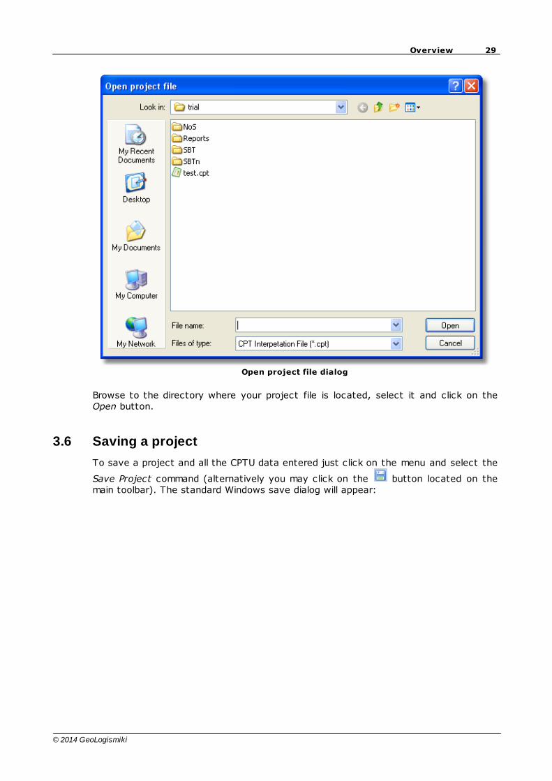
To load a previously saved project file, click on the File menu and select the Open
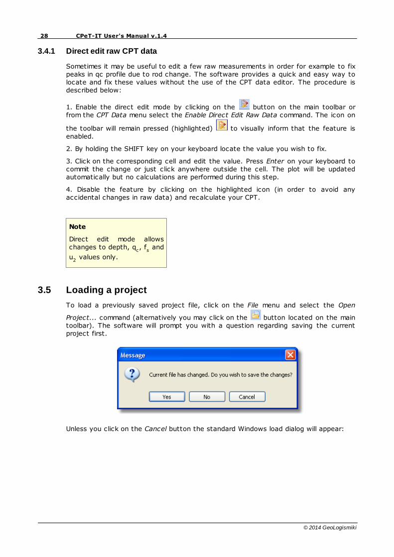
Project... command (alternatively you may click on the button located on the maintoolbar). The software will prompt you with a question regarding saving the currentproject first.
Unless you click on the Cancel button the standard Windows load dialog will appear:
29Overview
© 2014 GeoLogismiki
Open project file dialog
Browse to the directory where your project file is located, select it and click on theOpen button.
3.6 Saving a project
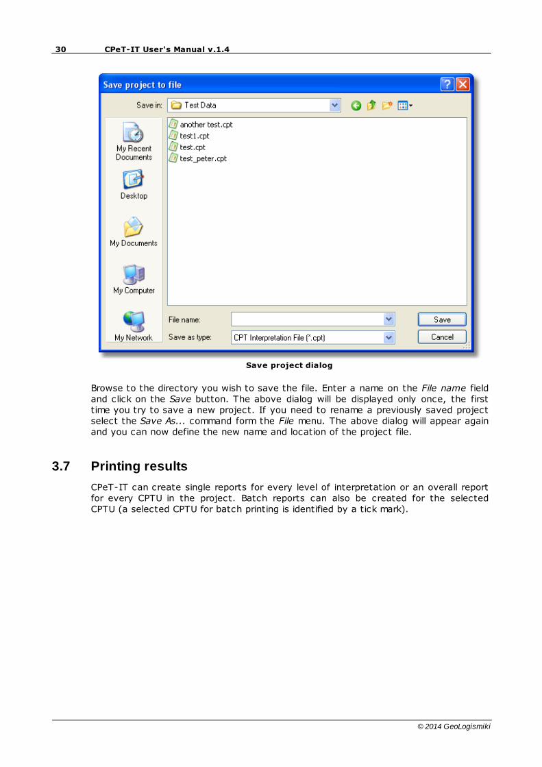
To save a project and all the CPTU data entered just click on the menu and select the
Save Project command (alternatively you may click on the button located on themain toolbar). The standard Windows save dialog will appear:
30 CPeT-IT User's Manual v.1.4
© 2014 GeoLogismiki
Save project dialog
Browse to the directory you wish to save the file. Enter a name on the File name fieldand click on the Save button. The above dialog will be displayed only once, the firsttime you try to save a new project. If you need to rename a previously saved projectselect the Save As... command form the File menu. The above dialog will appear againand you can now define the new name and location of the project file.
3.7 Printing results
CPeT-IT can create single reports for every level of interpretation or an overall reportfor every CPTU in the project. Batch reports can also be created for the selectedCPTU (a selected CPTU for batch printing is identified by a tick mark).
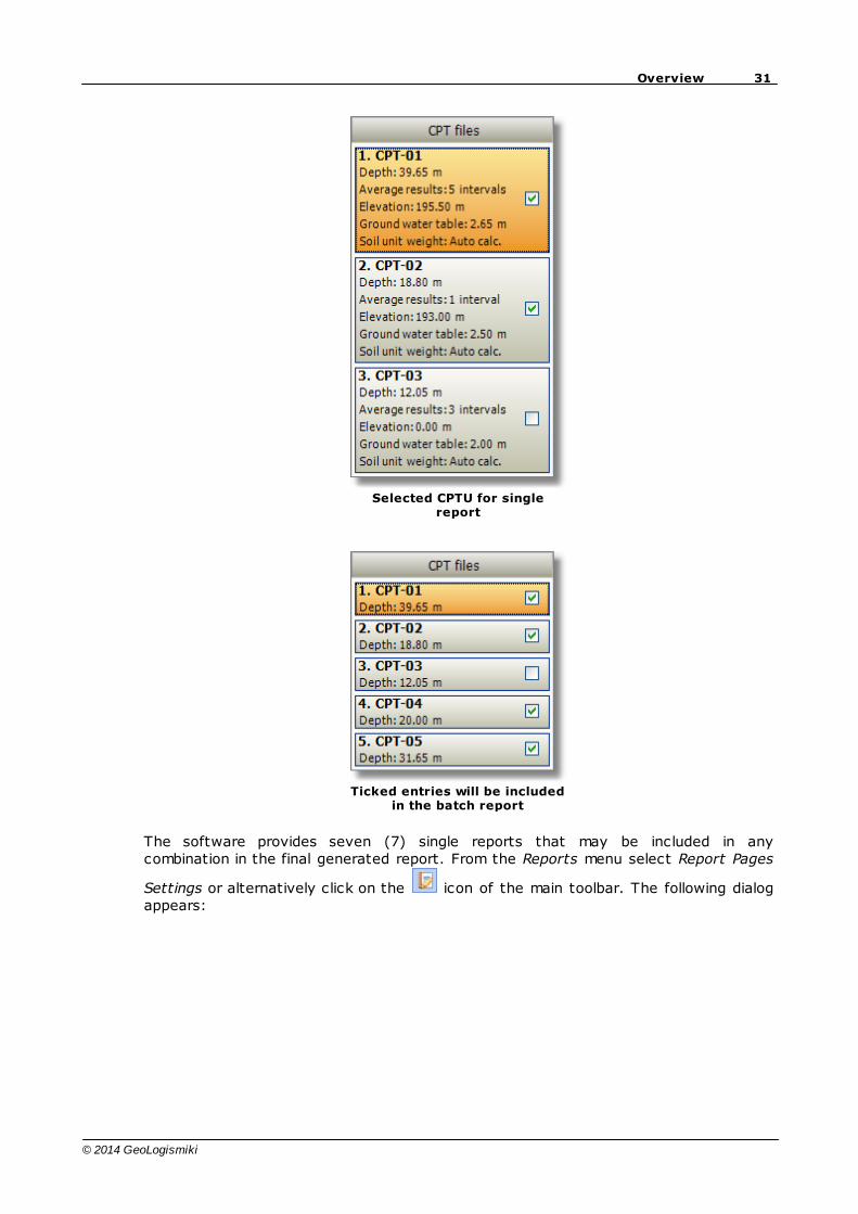
31Overview
© 2014 GeoLogismiki
Selected CPTU for singlereport
Ticked entries will be includedin the batch report
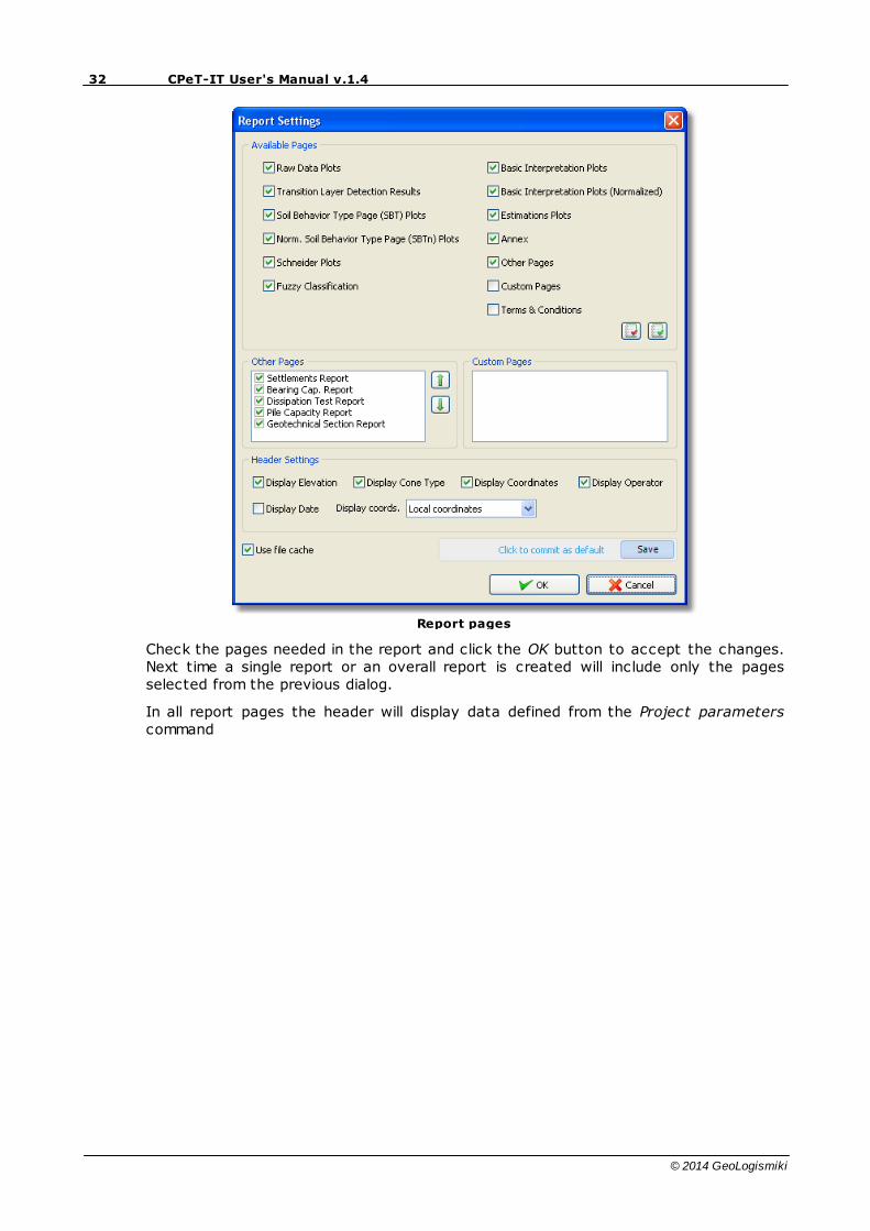
The software provides seven (7) single reports that may be included in anycombination in the final generated report. From the Reports menu select Report Pages
Settings or alternatively click on the icon of the main toolbar. The following dialogappears:
32 CPeT-IT User's Manual v.1.4
© 2014 GeoLogismiki
Report pages
Check the pages needed in the report and click the OK button to accept the changes.Next time a single report or an overall report is created will include only the pagesselected from the previous dialog.
In all report pages the header will display data defined from the Project parameterscommand
33Overview
© 2014 GeoLogismiki
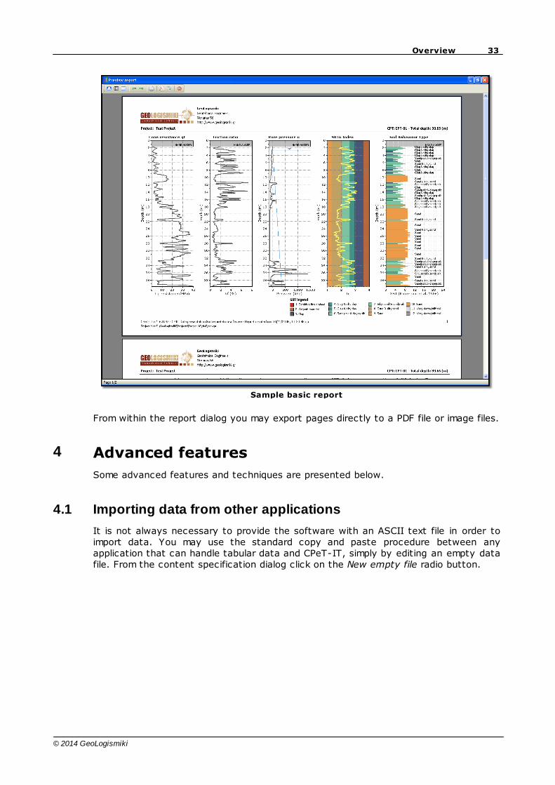
Sample basic report
From within the report dialog you may export pages directly to a PDF file or image files.
4 Advanced features
Some advanced features and techniques are presented below.
4.1 Importing data from other applications
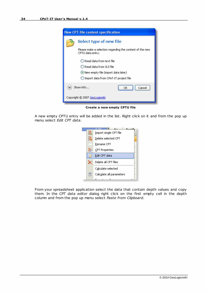
It is not always necessary to provide the software with an ASCII text file in order toimport data. You may use the standard copy and paste procedure between anyapplication that can handle tabular data and CPeT-IT, simply by editing an empty datafile. From the content specification dialog click on the New empty file radio button.
34 CPeT-IT User's Manual v.1.4
© 2014 GeoLogismiki
Create a new empty CPTU file
A new empty CPTU entry will be added in the list. Right click on it and from the pop upmenu select Edit CPT data.
From your spreadsheet application select the data that contain depth values and copythem. In the CPT data editor dialog right click on the first empty cell in the depthcolumn and from the pop up menu select Paste from Clipboard.
35Advanced features
© 2014 GeoLogismiki
The software will create as many rows as needed to fit all the data from memory.Repeat the same procedure for other values (cone resistance, sleeve friction an porepressure). You must always have in mind to paste data that comply with the projectunit system.
4.2 Adding sample data
Since it is possible to collect small diameter, disturbed soil samples with the same CPTpushing equipment immediately after the CPT, you may need to display this informationinside the raw cone resistance plot. Select a CPTU data and open the Edit CPT datacommand and click on the Samples tab located at the top of the dialog.
36 CPeT-IT User's Manual v.1.4
© 2014 GeoLogismiki
Samples tab in the CPT data editor
To insert a soil sample just click on the Add sample button and a new sample entry willappear at the end of the samples list. In the From edit box enter the depth fromwhere the sampling procedure began. In the To edit box enter the depth where thesampling procedure stopped. In the Start From edit box you may enter a value whichdenotes the relative distance to the plot width from where the sample will appear.Click on the color box to define a custom color for the sample.
To delete all samples from the current CPTU click on the Clear all button. To deleteonly the selected one click on the Delete selected button. Clicking on the UpdateSamples Only button will close the dialog and save only the samples information.
37Advanced features
© 2014 GeoLogismiki
4.3 Adding custom estimations data
It is possible to plot soil parameter data measured by other means like laboratory
tests, over the estimations plots from CPTu. Click on the icon located at the farright of the top toolbar and the following dialog will appear:
Custom estimations input dialog
Using the above displayed table enter depth and soil parameter values. When finishedcheck the Display Data in Plots checkbox and click the OK button. Custom estimationsdata will now be plotted over the CPTu estimations plot in red dotted line.
38 CPeT-IT User's Manual v.1.4
© 2014 GeoLogismiki
Custom estimations data
Estimations plots with custom data
4.4 Customizing Reports
To customize the interpretation report generated, click on the Report Pages Settings
command under the Reports menu or alternatively click on the button on the maintoolbar. The following dialog will appear:
39Advanced features
© 2014 GeoLogismiki
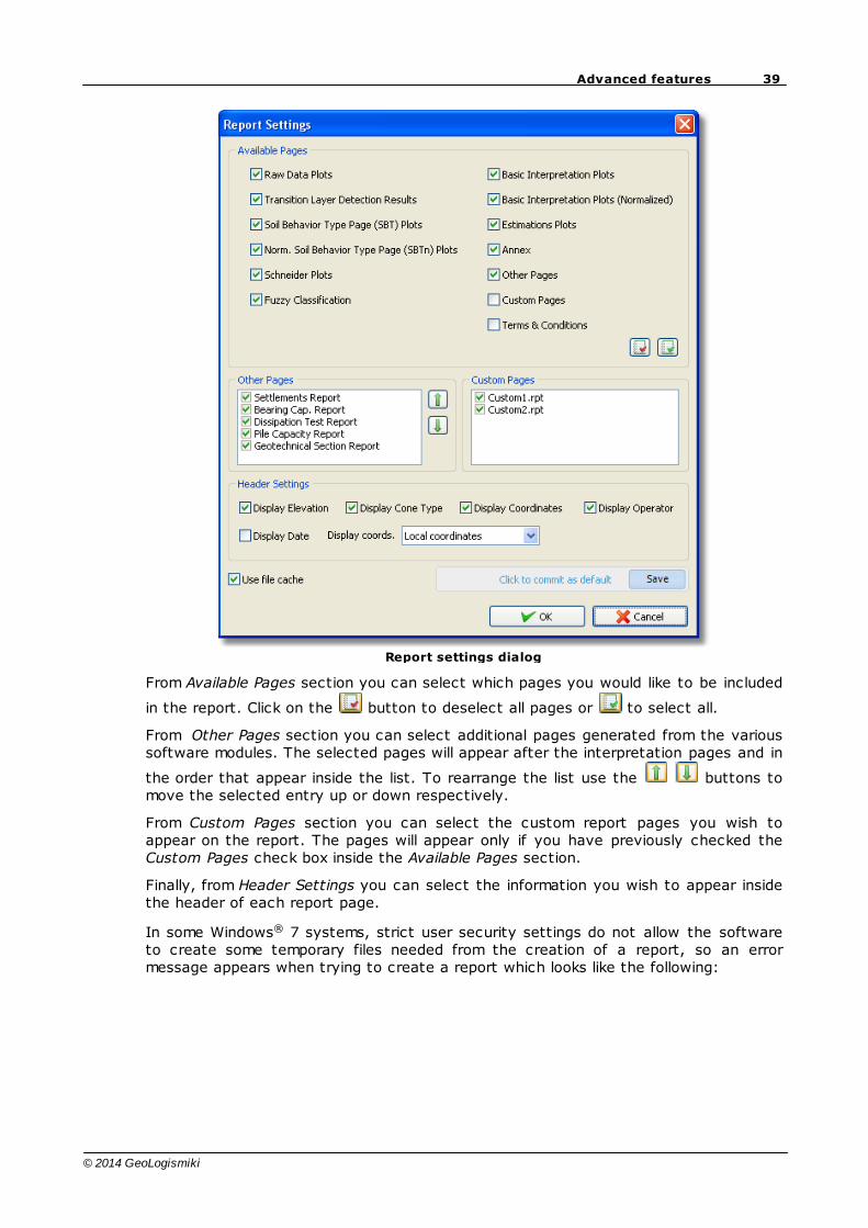
Report settings dialog
From Available Pages section you can select which pages you would like to be included
in the report. Click on the button to deselect all pages or to select all.
From Other Pages section you can select additional pages generated from the varioussoftware modules. The selected pages will appear after the interpretation pages and in
the order that appear inside the list. To rearrange the list use the buttons tomove the selected entry up or down respectively.
From Custom Pages section you can select the custom report pages you wish toappear on the report. The pages will appear only if you have previously checked theCustom Pages check box inside the Available Pages section.
Finally, from Header Settings you can select the information you wish to appear insidethe header of each report page.
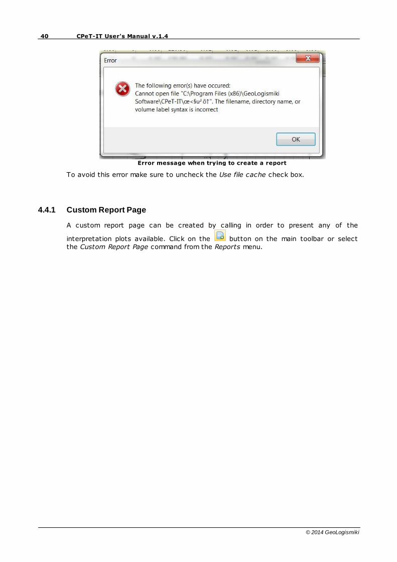
In some Windows® 7 systems, strict user security settings do not allow the softwareto create some temporary files needed from the creation of a report, so an errormessage appears when trying to create a report which looks like the following:
40 CPeT-IT User's Manual v.1.4
© 2014 GeoLogismiki
Error message when trying to create a report
To avoid this error make sure to uncheck the Use file cache check box.
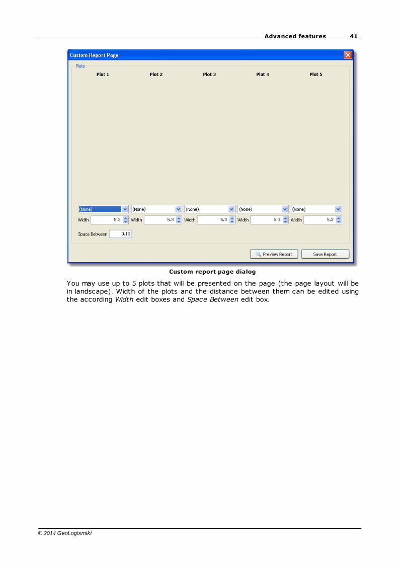
4.4.1 Custom Report Page
A custom report page can be created by calling in order to present any of the
interpretation plots available. Click on the button on the main toolbar or selectthe Custom Report Page command from the Reports menu.
41Advanced features
© 2014 GeoLogismiki
Custom report page dialog
You may use up to 5 plots that will be presented on the page (the page layout will bein landscape). Width of the plots and the distance between them can be edited usingthe according Width edit boxes and Space Between edit box.
42 CPeT-IT User's Manual v.1.4
© 2014 GeoLogismiki
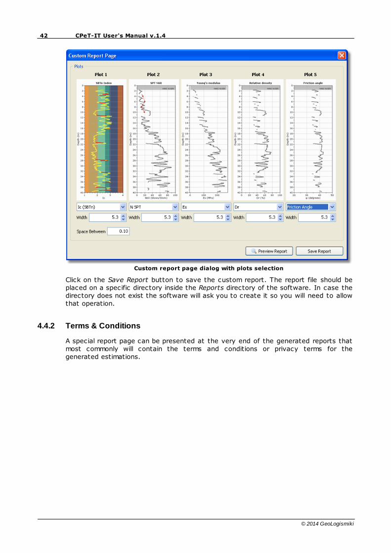
Custom report page dialog with plots selection
Click on the Save Report button to save the custom report. The report file should beplaced on a specific directory inside the Reports directory of the software. In case thedirectory does not exist the software will ask you to create it so you will need to allowthat operation.
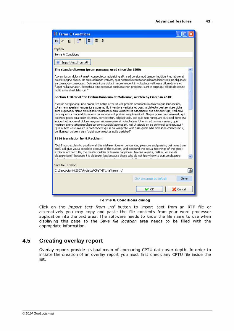
4.4.2 Terms & Conditions
A special report page can be presented at the very end of the generated reports thatmost commonly will contain the terms and conditions or privacy terms for thegenerated estimations.
43Advanced features
© 2014 GeoLogismiki
Terms & Conditions dialog
Click on the Import text from .rtf button to import text from an RTF file oralternatively you may copy and paste the file contents from your word processorapplication into the text area. The software needs to know the file name to use whendisplaying this page so the Save file location area needs to be filled with theappropriate information.
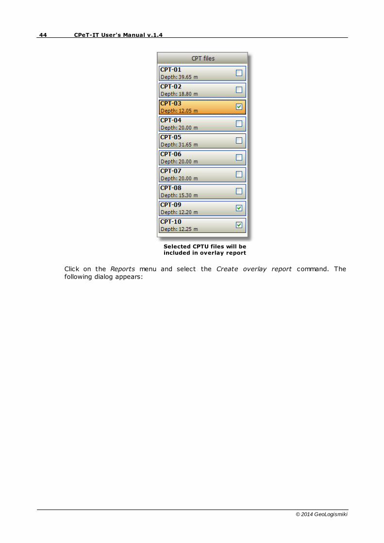
4.5 Creating overlay report
Overlay reports provide a visual mean of comparing CPTU data over depth. In order toinitiate the creation of an overlay report you must first check any CPTU file inside thelist.
44 CPeT-IT User's Manual v.1.4
© 2014 GeoLogismiki
Selected CPTU files will beincluded in overlay report
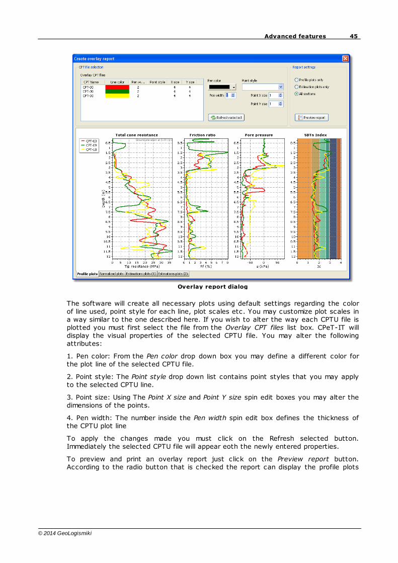
Click on the Reports menu and select the Create overlay report command. Thefollowing dialog appears:
45Advanced features
© 2014 GeoLogismiki
Overlay report dialog
The software will create all necessary plots using default settings regarding the colorof line used, point style for each line, plot scales etc. You may customize plot scales ina way similar to the one described here. If you wish to alter the way each CPTU file isplotted you must first select the file from the Overlay CPT files list box. CPeT-IT willdisplay the visual properties of the selected CPTU file. You may alter the followingattributes:
1. Pen color: From the Pen color drop down box you may define a different color forthe plot line of the selected CPTU file.
2. Point style: The Point style drop down list contains point styles that you may applyto the selected CPTU line.
3. Point size: Using The Point X size and Point Y size spin edit boxes you may alter thedimensions of the points.
4. Pen width: The number inside the Pen width spin edit box defines the thickness ofthe CPTU plot line
To apply the changes made you must click on the Refresh selected button.Immediately the selected CPTU file will appear eoth the newly entered properties.
To preview and print an overlay report just click on the Preview report button.According to the radio button that is checked the report can display the profile plots
46 CPeT-IT User's Manual v.1.4
© 2014 GeoLogismiki
only, the estimation plots only or profile and estimation plots.
4.6 Working with plots
4.6.1 Customizing plots
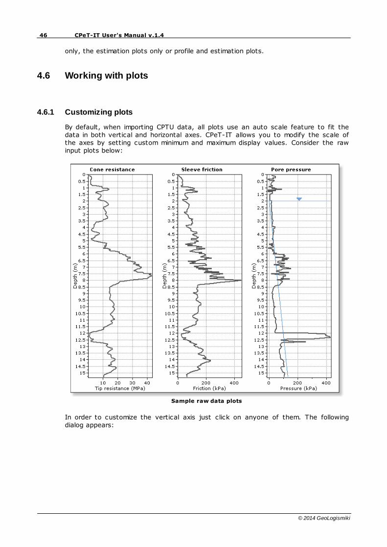
By default, when importing CPTU data, all plots use an auto scale feature to fit thedata in both vertical and horizontal axes. CPeT-IT allows you to modify the scale ofthe axes by setting custom minimum and maximum display values. Consider the rawinput plots below:
Sample raw data plots
In order to customize the vertical axis just click on anyone of them. The followingdialog appears:
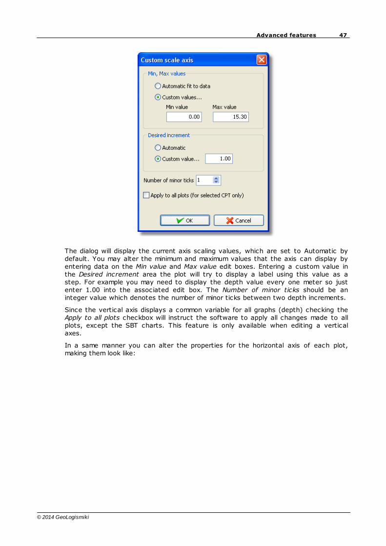
47Advanced features
© 2014 GeoLogismiki
The dialog will display the current axis scaling values, which are set to Automatic bydefault. You may alter the minimum and maximum values that the axis can display byentering data on the Min value and Max value edit boxes. Entering a custom value inthe Desired increment area the plot will try to display a label using this value as astep. For example you may need to display the depth value every one meter so justenter 1.00 into the associated edit box. The Number of minor ticks should be aninteger value which denotes the number of minor ticks between two depth increments.
Since the vertical axis displays a common variable for all graphs (depth) checking theApply to all plots checkbox will instruct the software to apply all changes made to allplots, except the SBT charts. This feature is only available when editing a verticalaxes.
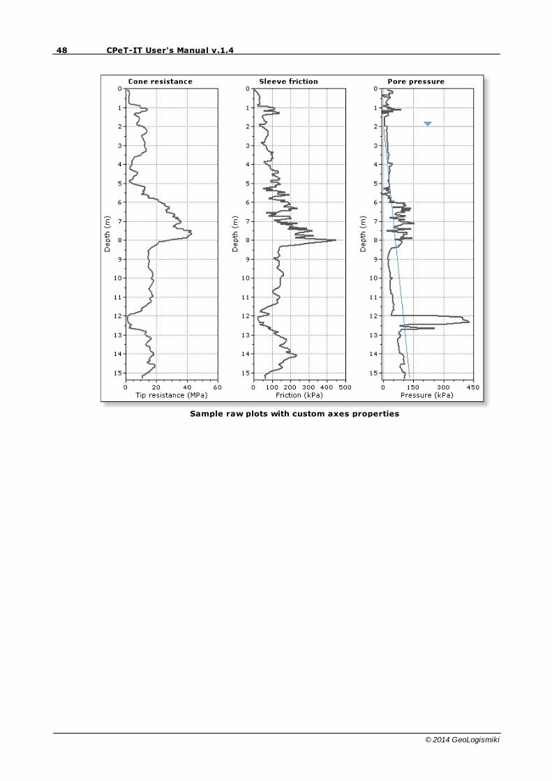
In a same manner you can alter the properties for the horizontal axis of each plot,making them look like:
48 CPeT-IT User's Manual v.1.4
© 2014 GeoLogismiki
Sample raw plots with custom axes properties
49Advanced features
© 2014 GeoLogismiki
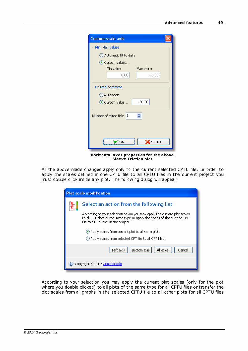
Horizontal axes properties for the aboveSleeve Friction plot
All the above made changes apply only to the current selected CPTU file. In order toapply the scales defined in one CPTU file to all CPTU files in the current project youmust double click inside any plot. The following dialog will appear:
According to your selection you may apply the current plot scales (only for the plotwhere you double clicked) to all plots of the same type for all CPTU files or transfer theplot scales from all graphs in the selected CPTU file to all other plots for all CPTU files
50 CPeT-IT User's Manual v.1.4
© 2014 GeoLogismiki
in the current project. You may also apply changes only for the left axes or bottomaxes or all axes.
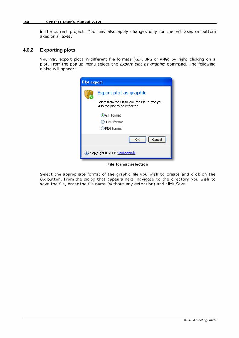
4.6.2 Exporting plots
You may export plots in different file formats (GIF, JPG or PNG) by right clicking on aplot. From the pop up menu select the Export plot as graphic command. The followingdialog will appear:
File format selection
Select the appropriate format of the graphic file you wish to create and click on theOK button. From the dialog that appears next, navigate to the directory you wish tosave the file, enter the file name (without any extension) and click Save.
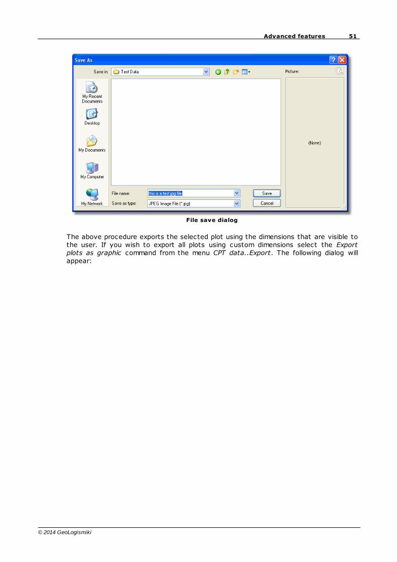
51Advanced features
© 2014 GeoLogismiki
File save dialog
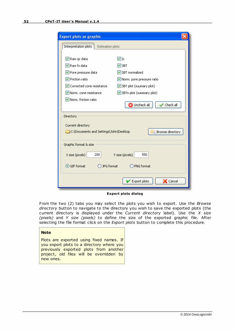
The above procedure exports the selected plot using the dimensions that are visible tothe user. If you wish to export all plots using custom dimensions select the Exportplots as graphic command from the menu CPT data..Export. The following dialog willappear:
52 CPeT-IT User's Manual v.1.4
© 2014 GeoLogismiki
Export plots dialog
From the two (2) tabs you may select the plots you wish to export. Use the Browsedirectory button to navigate to the directory you wish to save the exported plots (thecurrent directory is displayed under the Current directory label). Use the X size(pixels) and Y size (pixels) to define the size of the exported graphic file. Afterselecting the file format click on the Export plots button to complete this procedure.
Note
Plots are exported using fixed names. Ifyou export plots to a directory where youpreviously exported plots from anotherproject, old files will be overridden bynew ones.
53Advanced features
© 2014 GeoLogismiki
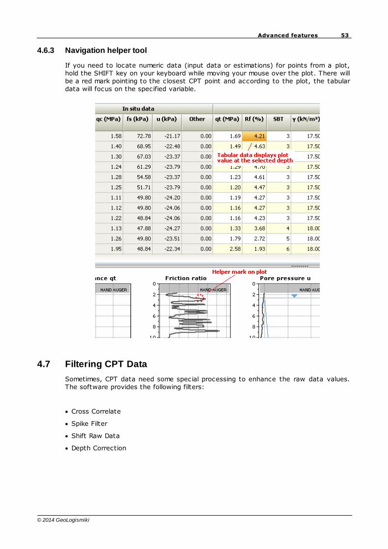
4.6.3 Navigation helper tool
If you need to locate numeric data (input data or estimations) for points from a plot,hold the SHIFT key on your keyboard while moving your mouse over the plot. There willbe a red mark pointing to the closest CPT point and according to the plot, the tabulardata will focus on the specified variable.
4.7 Filtering CPT Data
Sometimes, CPT data need some special processing to enhance the raw data values.The software provides the following filters:
Cross Correlate
Spike Filter
Shift Raw Data
Depth Correction
54 CPeT-IT User's Manual v.1.4
© 2014 GeoLogismiki
Negative Value
Convert u1 to u2
4.7.1 Cross Correlate
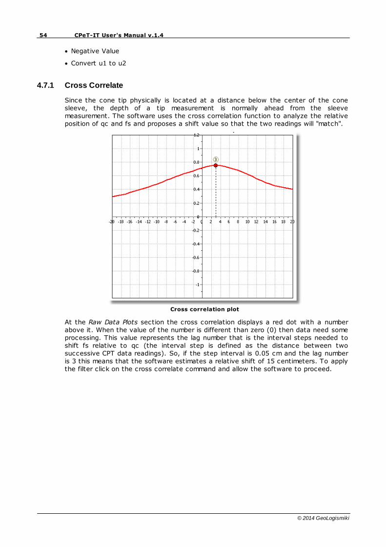
Since the cone tip physically is located at a distance below the center of the conesleeve, the depth of a tip measurement is normally ahead from the sleevemeasurement. The software uses the cross correlation function to analyze the relativeposition of qc and fs and proposes a shift value so that the two readings will "match".
Cross correlation plot
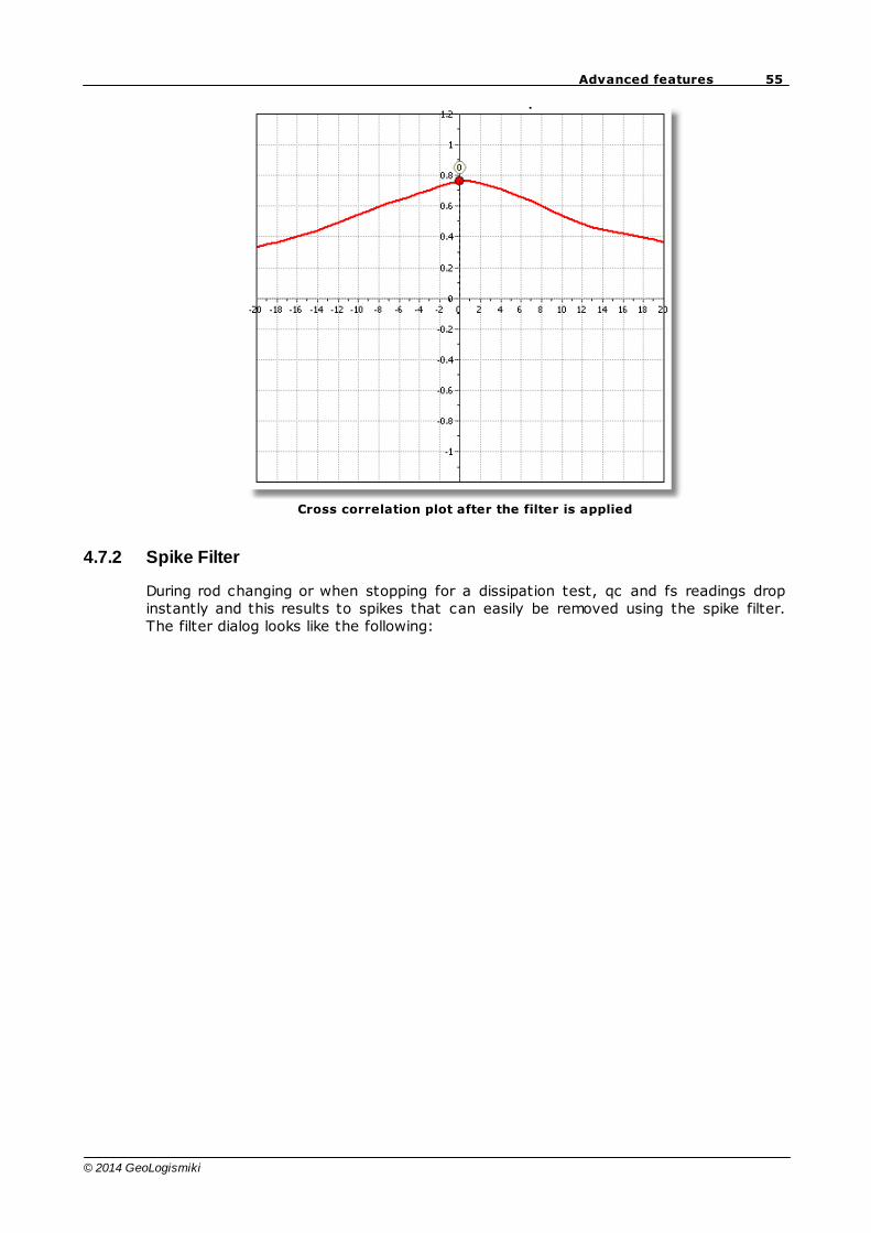
At the Raw Data Plots section the cross correlation displays a red dot with a numberabove it. When the value of the number is different than zero (0) then data need someprocessing. This value represents the lag number that is the interval steps needed toshift fs relative to qc (the interval step is defined as the distance between twosuccessive CPT data readings). So, if the step interval is 0.05 cm and the lag numberis 3 this means that the software estimates a relative shift of 15 centimeters. To applythe filter click on the cross correlate command and allow the software to proceed.
55Advanced features
© 2014 GeoLogismiki
Cross correlation plot after the filter is applied
4.7.2 Spike Filter
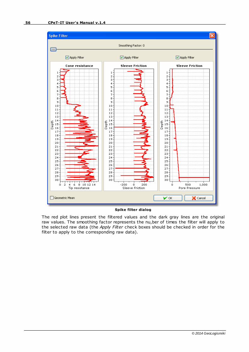
During rod changing or when stopping for a dissipation test, qc and fs readings dropinstantly and this results to spikes that can easily be removed using the spike filter.The filter dialog looks like the following:
56 CPeT-IT User's Manual v.1.4
© 2014 GeoLogismiki
Spike filter dialog
The red plot lines present the filtered values and the dark gray lines are the originalraw values. The smoothing factor represents the nu,ber of times the filter will apply tothe selected raw data (the Apply Filter check boxes should be checked in order for thefilter to apply to the corresponding raw data).
57Advanced features
© 2014 GeoLogismiki
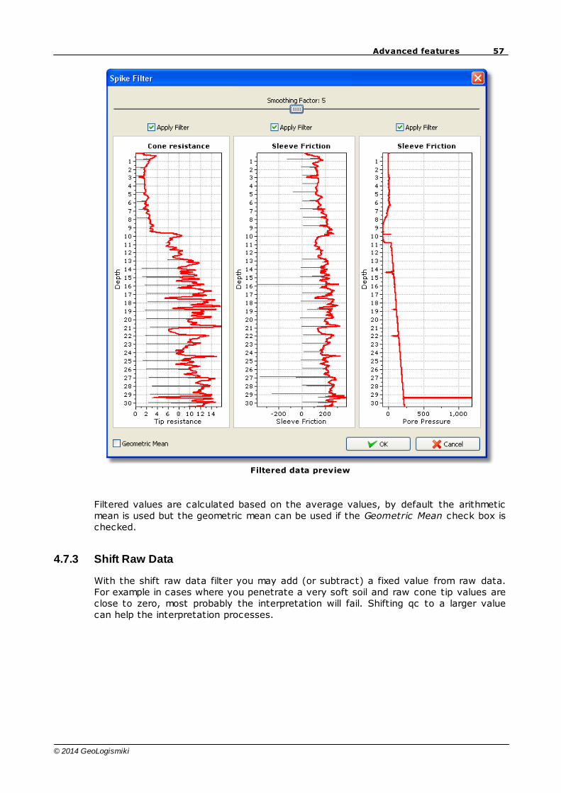
Filtered data preview
Filtered values are calculated based on the average values, by default the arithmeticmean is used but the geometric mean can be used if the Geometric Mean check box ischecked.
4.7.3 Shift Raw Data
With the shift raw data filter you may add (or subtract) a fixed value from raw data.For example in cases where you penetrate a very soft soil and raw cone tip values areclose to zero, most probably the interpretation will fail. Shifting qc to a larger valuecan help the interpretation processes.
58 CPeT-IT User's Manual v.1.4
© 2014 GeoLogismiki
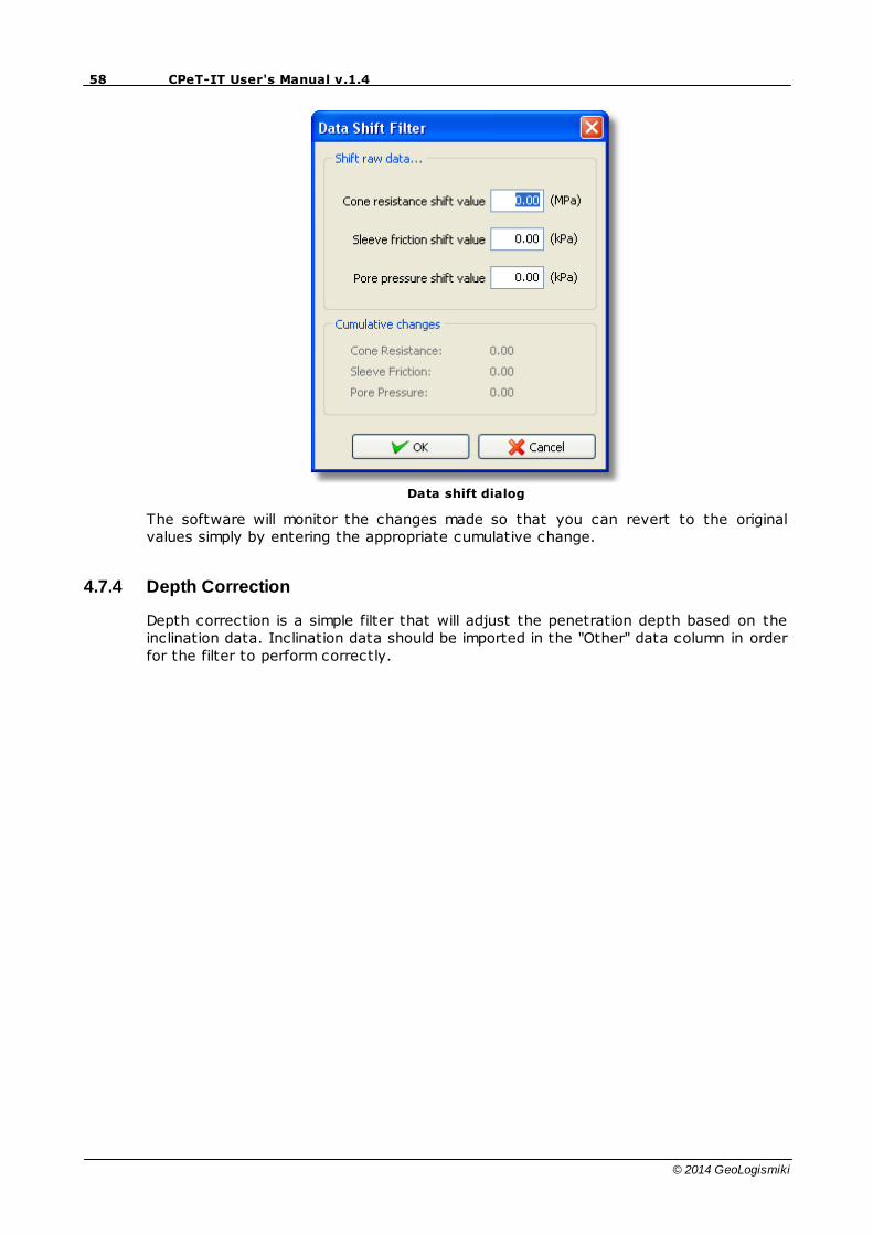
Data shift dialog
The software will monitor the changes made so that you can revert to the originalvalues simply by entering the appropriate cumulative change.
4.7.4 Depth Correction
Depth correction is a simple filter that will adjust the penetration depth based on theinclination data. Inclination data should be imported in the "Other" data column in orderfor the filter to perform correctly.
59Advanced features
© 2014 GeoLogismiki
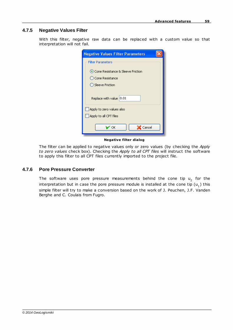
4.7.5 Negative Values Filter
With this filter, negative raw data can be replaced with a custom value so thatinterpretation will not fail.
Negative filter dialog
The filter can be applied to negative values only or zero values (by checking the Applyto zero values check box). Checking the Apply to all CPT files will instruct the softwareto apply this filter to all CPT files currently imported to the project file.
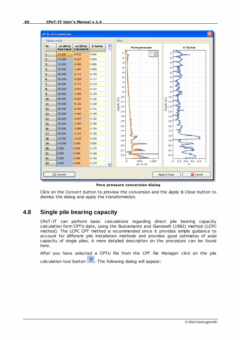
4.7.6 Pore Pressure Converter
The software uses pore pressure measurements behind the cone tip u2
for the
interpretation but in case the pore pressure module is installed at the cone tip (u1) this
simple filter will try to make a conversion based on the work of J. Peuchen, J.F. VandenBerghe and C. Coulais from Fugro.
60 CPeT-IT User's Manual v.1.4
© 2014 GeoLogismiki
Pore pressure conversion dialog
Click on the Convert button to preview the conversion and the Apply & Close button todismiss the dialog and apply the transformation.
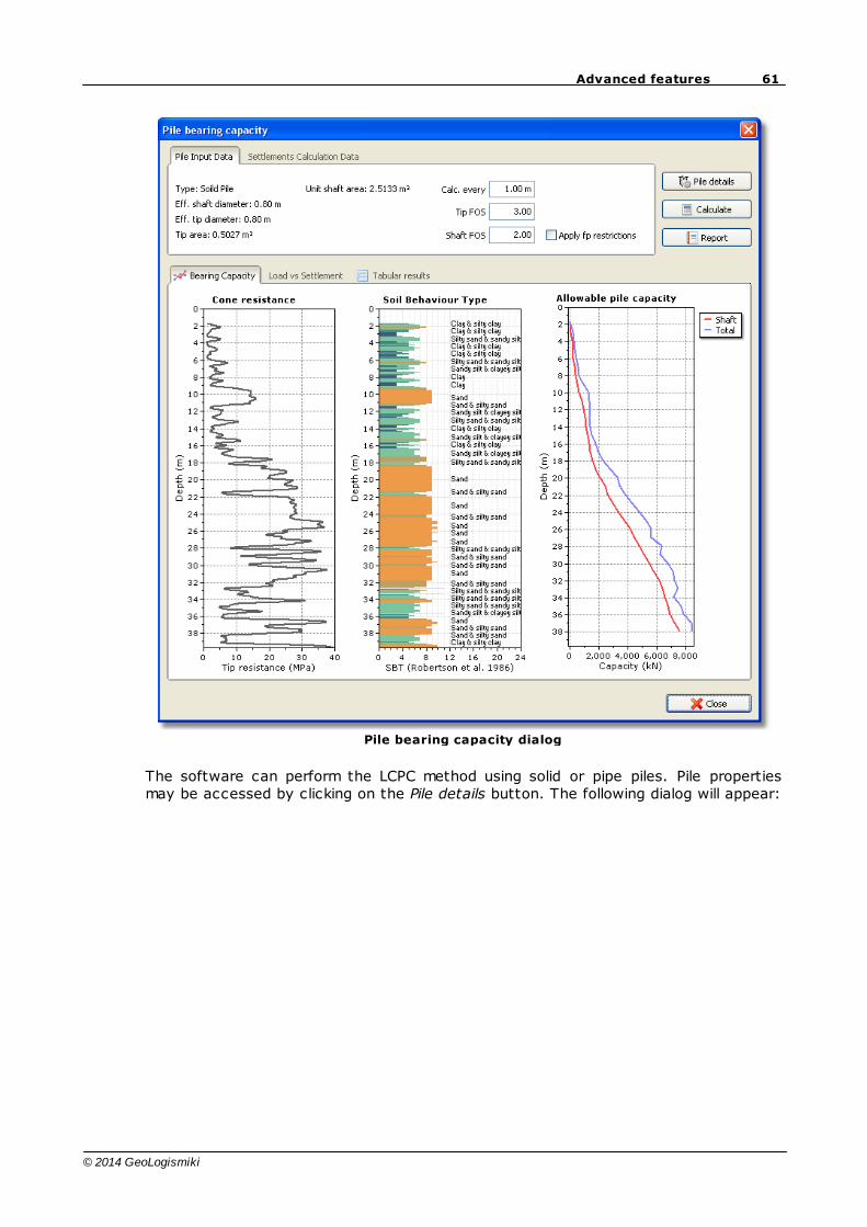
4.8 Single pile bearing capacity
CPeT-IT can perform basic calculations regarding direct pile bearing capacitycalculation form CPTU data, using the Bustamante and Gianaselli (1982) method (LCPCmethod). The LCPC CPT method is recommended since it provides simple guidance toaccount for different pile installation methods and provides good estimates of axialcapacity of single piles. A more detailed description on the procedure can be foundhere.
After you have selected a CPTU file from the CPT file Manager click on the pile
calculation tool button . The following dialog will appear:
61Advanced features
© 2014 GeoLogismiki
Pile bearing capacity dialog
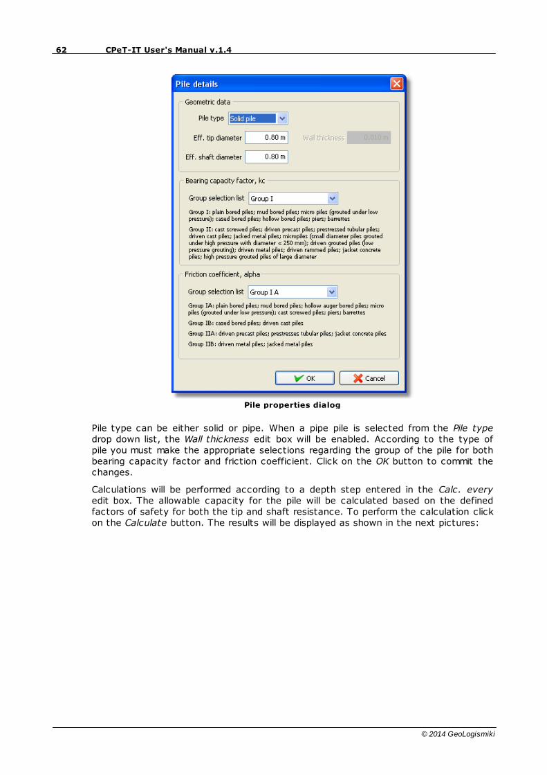
The software can perform the LCPC method using solid or pipe piles. Pile propertiesmay be accessed by clicking on the Pile details button. The following dialog will appear:
62 CPeT-IT User's Manual v.1.4
© 2014 GeoLogismiki
Pile properties dialog
Pile type can be either solid or pipe. When a pipe pile is selected from the Pile typedrop down list, the Wall thickness edit box will be enabled. According to the type ofpile you must make the appropriate selections regarding the group of the pile for bothbearing capacity factor and friction coefficient. Click on the OK button to commit thechanges.
Calculations will be performed according to a depth step entered in the Calc. everyedit box. The allowable capacity for the pile will be calculated based on the definedfactors of safety for both the tip and shaft resistance. To perform the calculation clickon the Calculate button. The results will be displayed as shown in the next pictures:
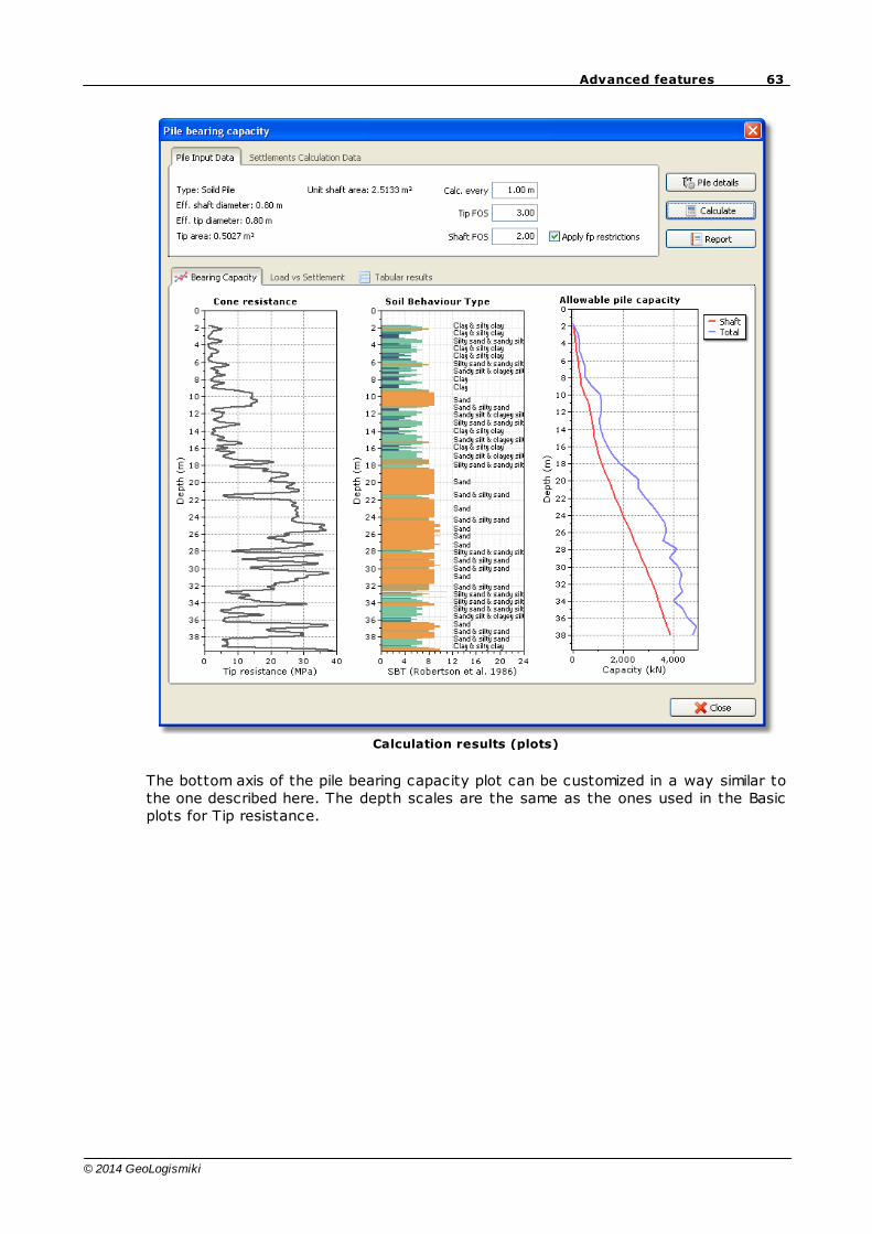
63Advanced features
© 2014 GeoLogismiki
Calculation results (plots)
The bottom axis of the pile bearing capacity plot can be customized in a way similar tothe one described here. The depth scales are the same as the ones used in the Basicplots for Tip resistance.
64 CPeT-IT User's Manual v.1.4
© 2014 GeoLogismiki
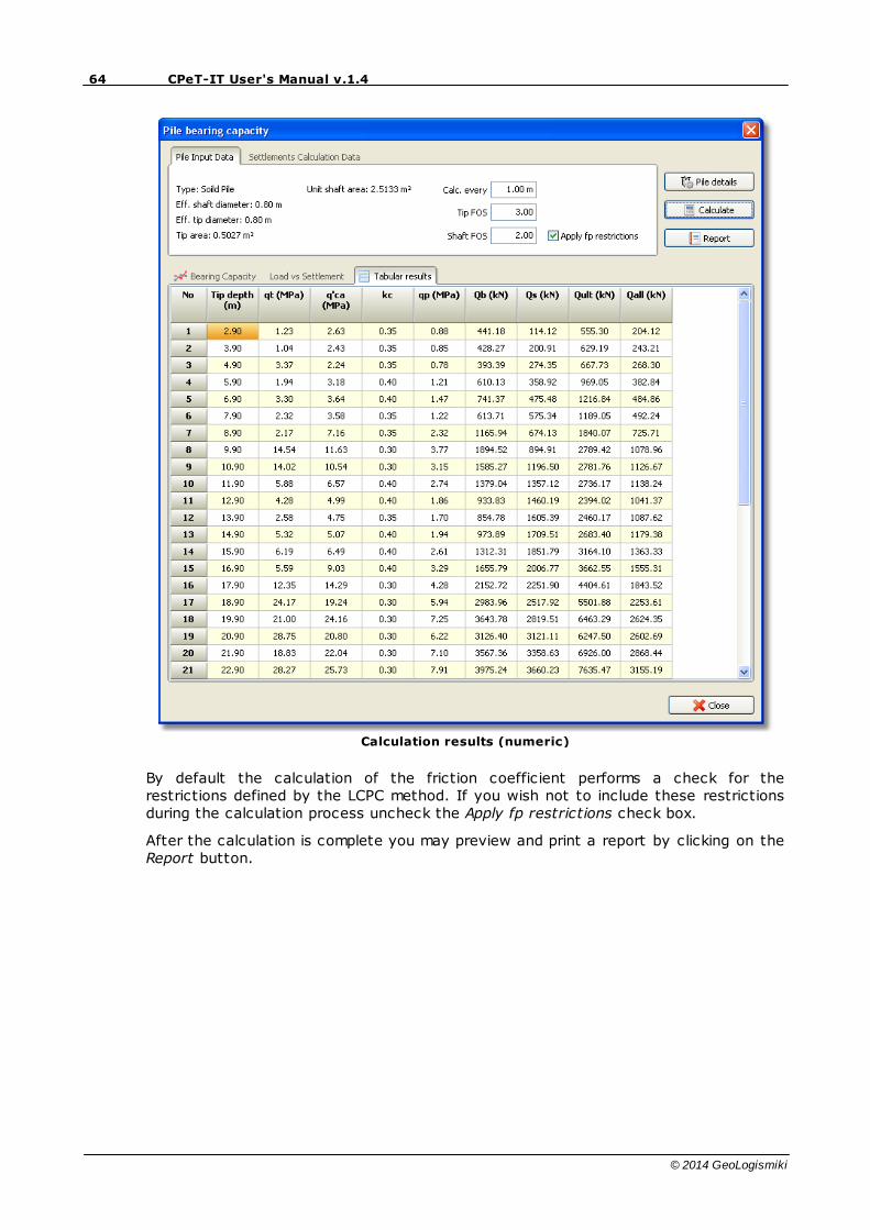
Calculation results (numeric)
By default the calculation of the friction coefficient performs a check for therestrictions defined by the LCPC method. If you wish not to include these restrictionsduring the calculation process uncheck the Apply fp restrictions check box.
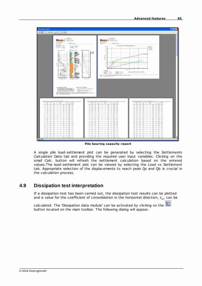
After the calculation is complete you may preview and print a report by clicking on theReport button.
65Advanced features
© 2014 GeoLogismiki
Pile bearing capacity report
A single pile load-settlement plot can be generated by selecting the SettlementsCalculation Data tab and providing the required user input variables. Clicking on thesmall Calc. button will refresh the settlement calculation based on the enteredvalues.The load-settlement plot can be viewed by selecting the Load vs Settlementtab. Appropriate selection of the displacements to reach peak Qs and Qb is crucial inthe calculation process.
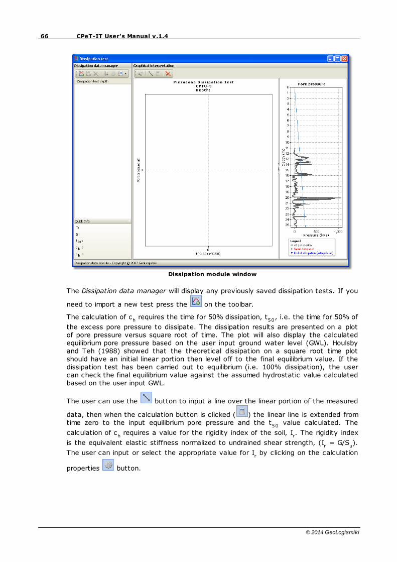
4.9 Dissipation test interpretation
If a dissipation test has been carried out, the dissipation test results can be plottedand a value for the coefficient of consolidation in the horizontal direction, c
h, can be
calculated. The 'Dissipation data module' can be activated by clicking on the button located on the main toolbar. The following dialog will appear.
66 CPeT-IT User's Manual v.1.4
© 2014 GeoLogismiki
Dissipation module window
The Dissipation data manager will display any previously saved dissipation tests. If you
need to import a new test press the on the toolbar.
The calculation of ch requires the time for 50% dissipation, t
50, i.e. the time for 50% of
the excess pore pressure to dissipate. The dissipation results are presented on a plotof pore pressure versus square root of time. The plot will also display the calculatedequilibrium pore pressure based on the user input ground water level (GWL). Houlsbyand Teh (1988) showed that the theoretical dissipation on a square root time plotshould have an initial linear portion then level off to the final equilibrium value. If thedissipation test has been carried out to equilibrium (i.e. 100% dissipation), the usercan check the final equilibrium value against the assumed hydrostatic value calculatedbased on the user input GWL.
The user can use the button to input a line over the linear portion of the measured
data, then when the calculation button is clicked ( ) the linear line is extended fromtime zero to the input equilibrium pore pressure and the t
50 value calculated. The
calculation of ch requires a value for the rigidity index of the soil, I
r. The rigidity index
is the equivalent elastic stiffness normalized to undrained shear strength, (Ir = G/S
u).
The user can input or select the appropriate value for Ir by clicking on the calculation
properties button.
67Advanced features
© 2014 GeoLogismiki
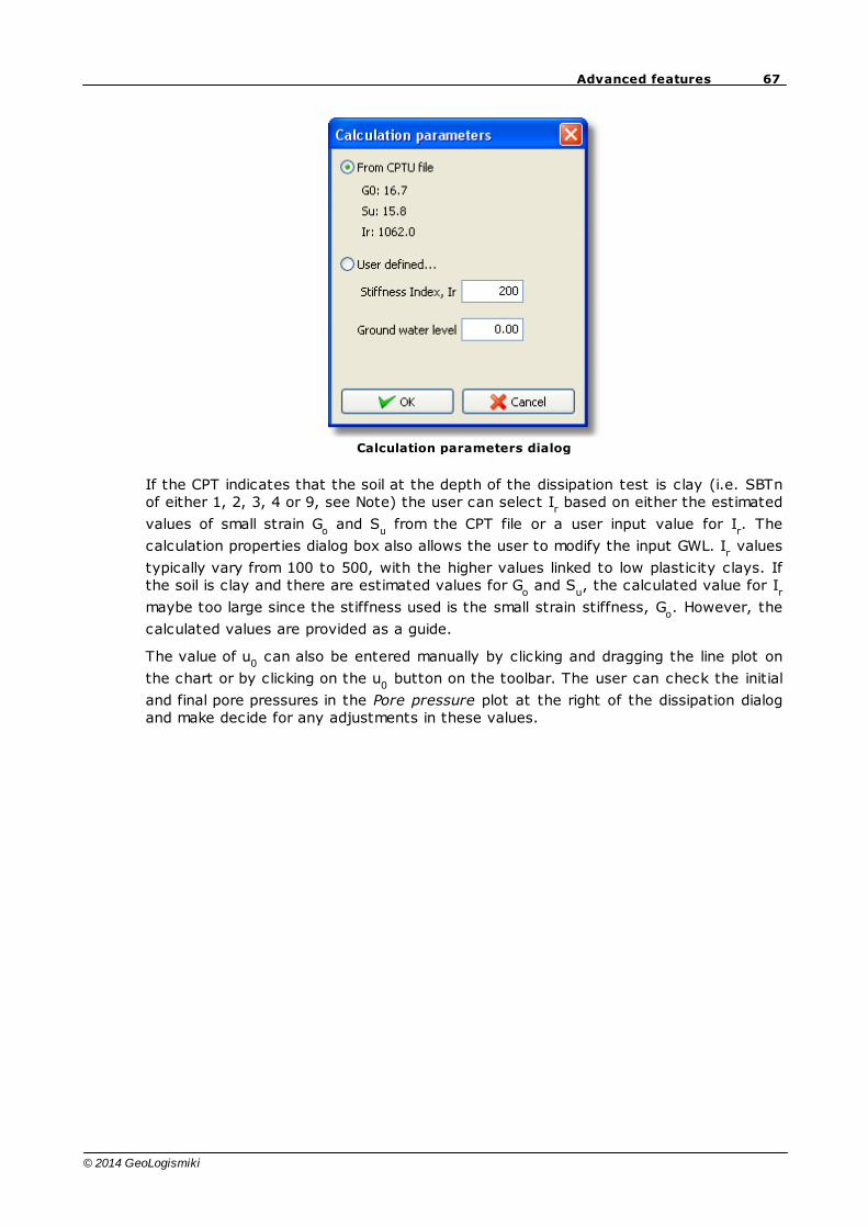
Calculation parameters dialog
If the CPT indicates that the soil at the depth of the dissipation test is clay (i.e. SBTnof either 1, 2, 3, 4 or 9, see Note) the user can select I
r based on either the estimated
values of small strain Go and S
u from the CPT file or a user input value for I
r. The
calculation properties dialog box also allows the user to modify the input GWL. Ir values
typically vary from 100 to 500, with the higher values linked to low plasticity clays. Ifthe soil is clay and there are estimated values for G
o and S
u, the calculated value for I
r
maybe too large since the stiffness used is the small strain stiffness, Go. However, the
calculated values are provided as a guide.
The value of u0 can also be entered manually by clicking and dragging the line plot on
the chart or by clicking on the u0 button on the toolbar. The user can check the initial
and final pore pressures in the Pore pressure plot at the right of the dissipation dialogand make decide for any adjustments in these values.
68 CPeT-IT User's Manual v.1.4
© 2014 GeoLogismiki
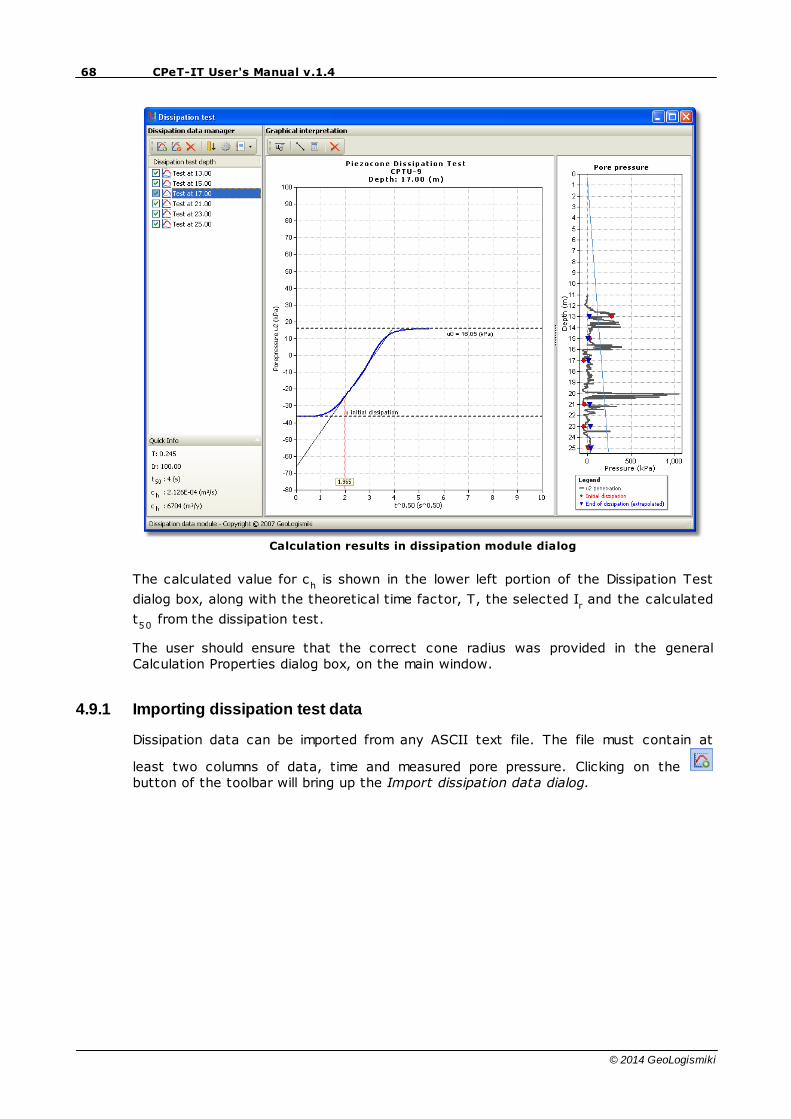
Calculation results in dissipation module dialog
The calculated value for ch is shown in the lower left portion of the Dissipation Test
dialog box, along with the theoretical time factor, T, the selected Ir and the calculated
t50
from the dissipation test.
The user should ensure that the correct cone radius was provided in the generalCalculation Properties dialog box, on the main window.
4.9.1 Importing dissipation test data
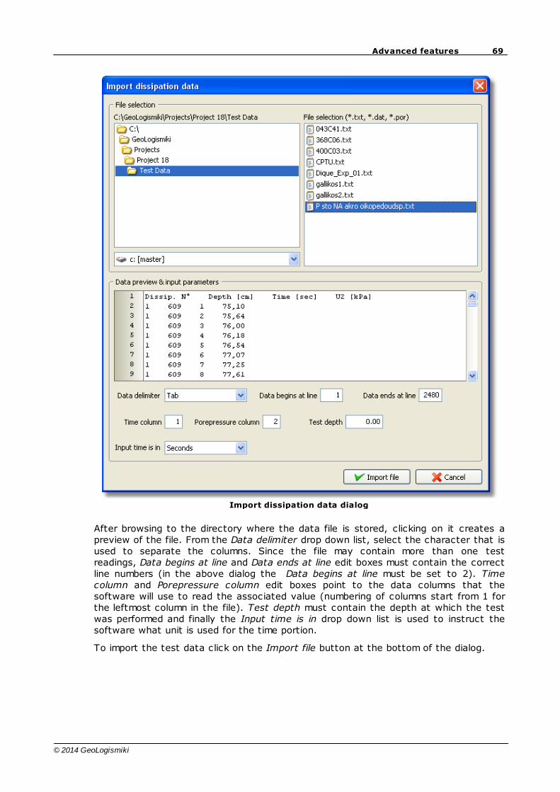
Dissipation data can be imported from any ASCII text file. The file must contain at
least two columns of data, time and measured pore pressure. Clicking on the button of the toolbar will bring up the Import dissipation data dialog.
69Advanced features
© 2014 GeoLogismiki
Import dissipation data dialog
After browsing to the directory where the data file is stored, clicking on it creates apreview of the file. From the Data delimiter drop down list, select the character that isused to separate the columns. Since the file may contain more than one testreadings, Data begins at line and Data ends at line edit boxes must contain the correctline numbers (in the above dialog the Data begins at line must be set to 2). Timecolumn and Porepressure column edit boxes point to the data columns that thesoftware will use to read the associated value (numbering of columns start from 1 forthe leftmost column in the file). Test depth must contain the depth at which the testwas performed and finally the Input time is in drop down list is used to instruct thesoftware what unit is used for the time portion.
To import the test data click on the Import file button at the bottom of the dialog.
70 CPeT-IT User's Manual v.1.4
© 2014 GeoLogismiki
4.10 Settlements calculation
CPTu data can be used to directly estimate induced settlements due to an externalload. CpeT-IT uses the following simple formula (based on 1-D consolidation) toestimate vertical settlements:
CPT
z
M
Ihqs
where:
q: applied footing pressure
h: calculation layer thickness
Iz: stress reduction factor according to Boussinesq
MC PT
: Constrained modulus of soil layer
After you have selected a CPTU file from the CPT file Manager click on then
settlements calculation tool button . The following dialog will appear:
71Advanced features
© 2014 GeoLogismiki
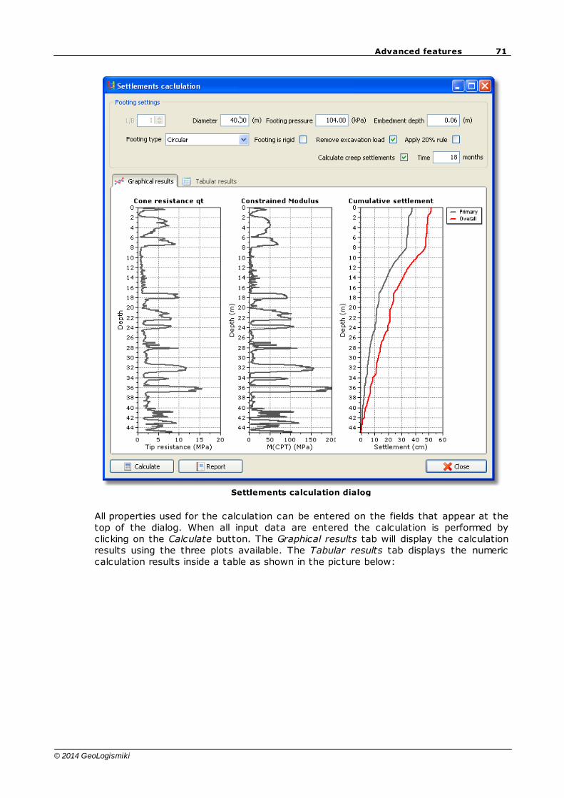
Settlements calculation dialog
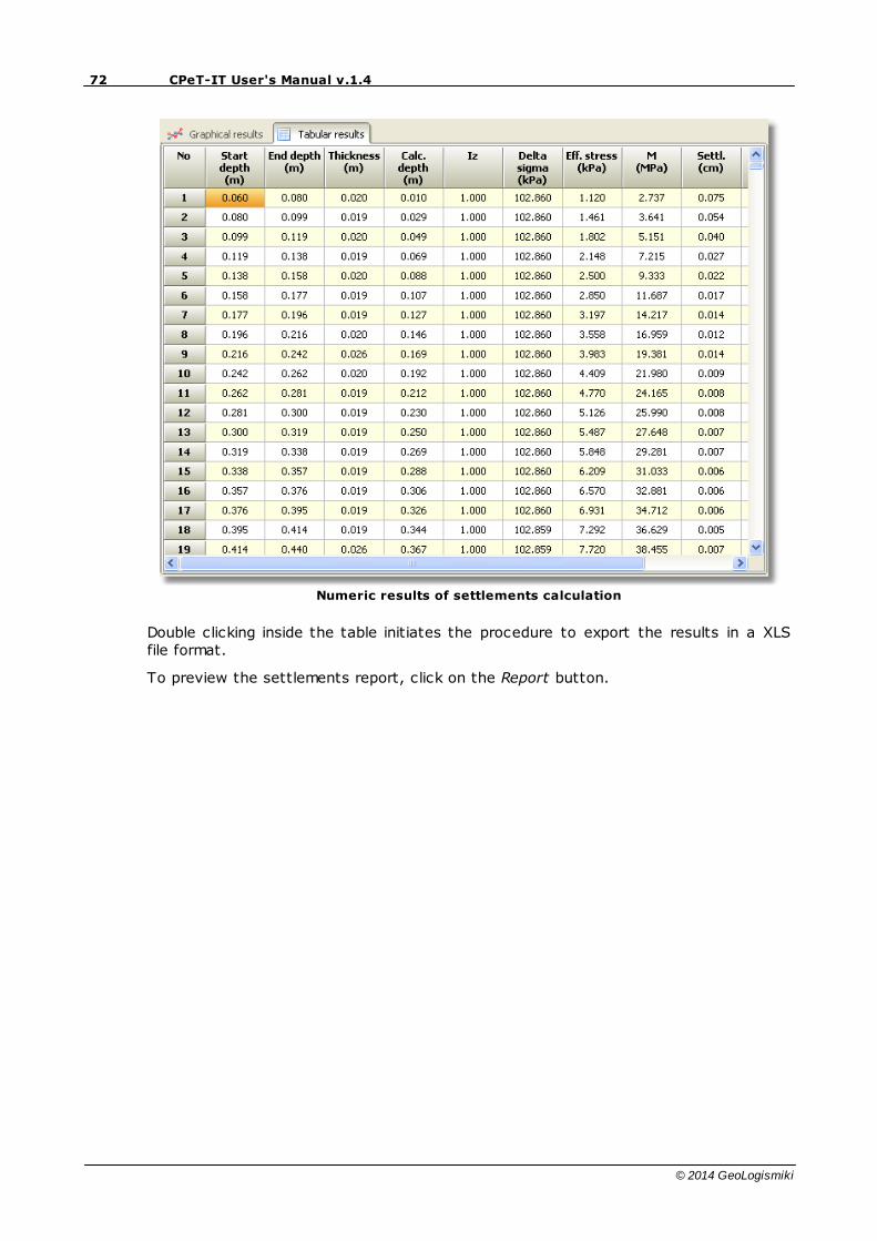
All properties used for the calculation can be entered on the fields that appear at thetop of the dialog. When all input data are entered the calculation is performed byclicking on the Calculate button. The Graphical results tab will display the calculationresults using the three plots available. The Tabular results tab displays the numericcalculation results inside a table as shown in the picture below:
72 CPeT-IT User's Manual v.1.4
© 2014 GeoLogismiki
Numeric results of settlements calculation
Double clicking inside the table initiates the procedure to export the results in a XLSfile format.
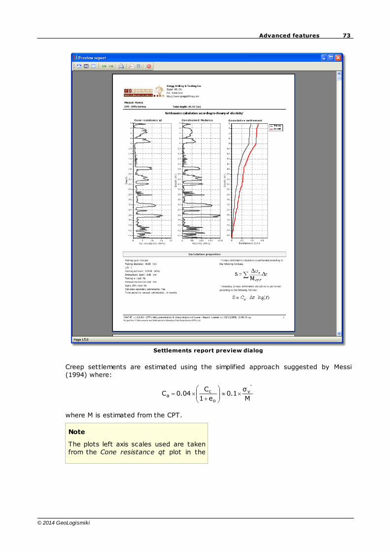
To preview the settlements report, click on the Report button.
73Advanced features
© 2014 GeoLogismiki
Settlements report preview dialog
Creep settlements are estimated using the simplified approach suggested by Messi(1994) where:
M
σ0.1
e1
C0.04C
'v
o
ca
where M is estimated from the CPT.
Note
The plots left axis scales used are takenfrom the Cone resistance qt plot in the
74 CPeT-IT User's Manual v.1.4
© 2014 GeoLogismiki
Basic plots tab of the main applicationwindow.
4.11 Geotechnical section creation
CPeT-IT offers a 2 modules for the creation of a typical geotechnical section, derivedfrom the CPT data. A semi auto boundaries detection and a manual layers definition areavailable for the user. The description below refers to the manual layer definitionmodule where using the mouse and/or keyboard the user can identify soil layers andcalculate the average estimated parameters (a description for semi auto module canbe found here). After you have selected a CPTU file from the CPT file Manager click on
then settlements calculation tool button . The following dialog will appear:
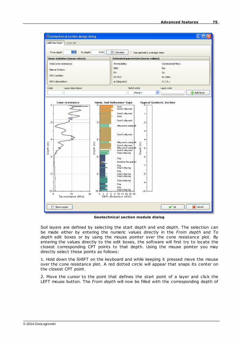
75Advanced features
© 2014 GeoLogismiki
Geotechnical section module dialog
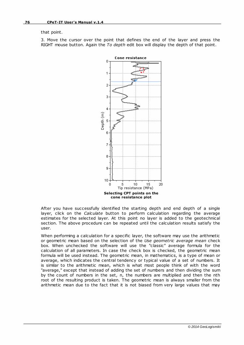
Soil layers are defined by selecting the start depth and end depth. The selection canbe made either by entering the numeric values directly in the From depth and Todepth edit boxes or by using the mouse pointer over the cone resistance plot. Byentering the values directly to the edit boxes, the software will first try to locate theclosest corresponding CPT points to that depth. Using the mouse pointer you maydirectly select these points as follows:
1. Hold down the SHIFT on the keyboard and while keeping it pressed move the mouseover the cone resistance plot. A red dotted circle will appear that snaps its center onthe closest CPT point.
2. Move the cursor to the point that defines the start point of a layer and click theLEFT mouse button. The From depth will now be filled with the corresponding depth of
76 CPeT-IT User's Manual v.1.4
© 2014 GeoLogismiki
that point.
3. Move the cursor over the point that defines the end of the layer and press theRIGHT mouse button. Again the To depth edit box will display the depth of that point.
Selecting CPT points on thecone resistance plot
After you have successfully identified the starting depth and end depth of a singlelayer, click on the Calculate button to perform calculation regarding the averageestimates for the selected layer. At this point no layer is added to the geotechnicalsection. The above procedure can be repeated until the calculation results satisfy theuser.
When performing a calculation for a specific layer, the software may use the arithmeticor geometric mean based on the selection of the Use geometric average mean checkbox. When unchecked the software will use the "classic" average formula for thecalculation of all parameters. In case the check box is checked, the geometric meanformula will be used instead. The geometric mean, in mathematics, is a type of mean oraverage, which indicates the central tendency or typical value of a set of numbers. Itis similar to the arithmetic mean, which is what most people think of with the word"average," except that instead of adding the set of numbers and then dividing the sumby the count of numbers in the set, n, the numbers are multiplied and then the nthroot of the resulting product is taken. The geometric mean is always smaller from thearithmetic mean due to the fact that it is not biased from very large values that may
77Advanced features
© 2014 GeoLogismiki
exist in a set. In order to produce a value greater than zero all of the numbers in theset should be greater than zero.
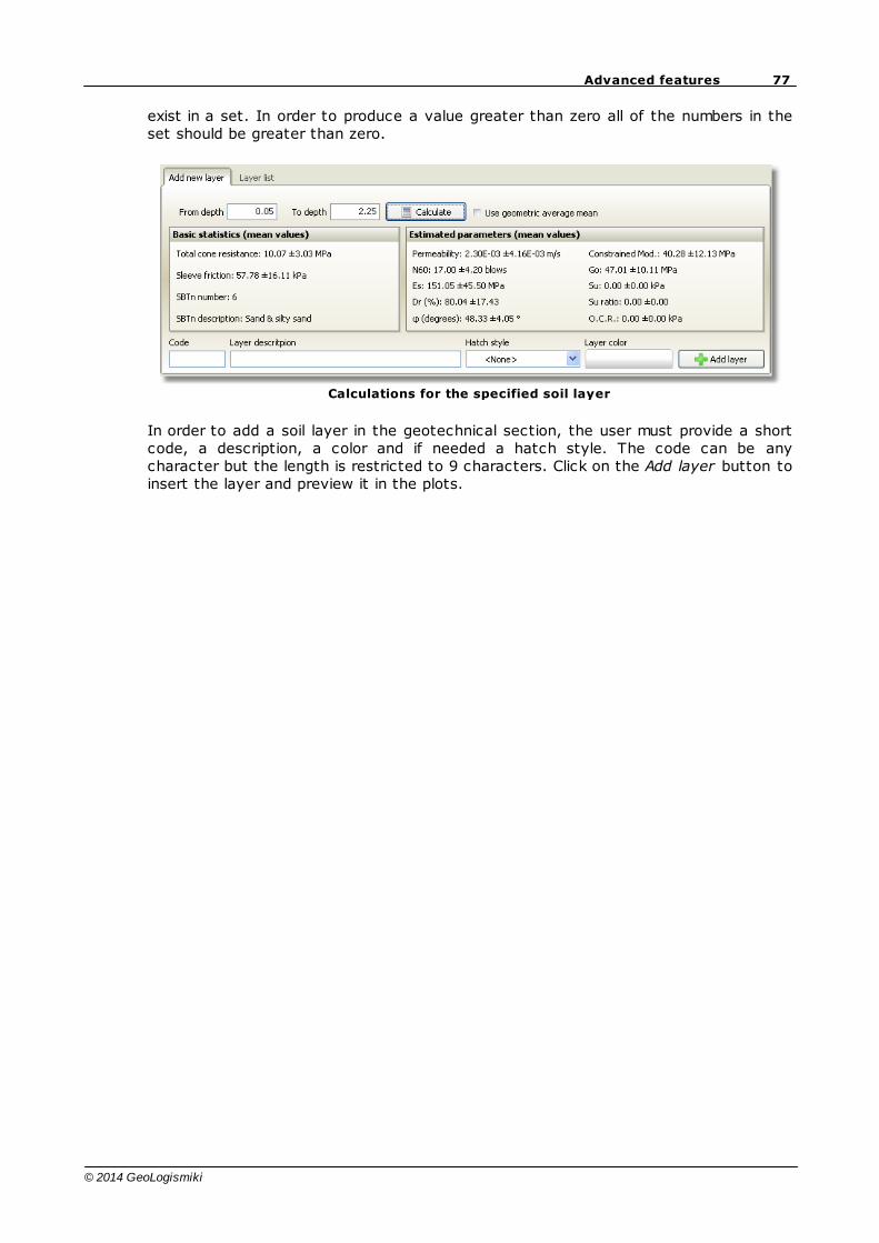
Calculations for the specified soil layer
In order to add a soil layer in the geotechnical section, the user must provide a shortcode, a description, a color and if needed a hatch style. The code can be anycharacter but the length is restricted to 9 characters. Click on the Add layer button toinsert the layer and preview it in the plots.
78 CPeT-IT User's Manual v.1.4
© 2014 GeoLogismiki
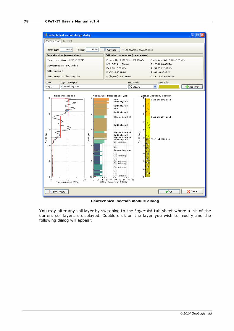
Geotechnical section module dialog
You may alter any soil layer by switching to the Layer list tab sheet where a list of thecurrent soil layers is displayed. Double click on the layer you wish to modify and thefollowing dialog will appear:
79Advanced features
© 2014 GeoLogismiki
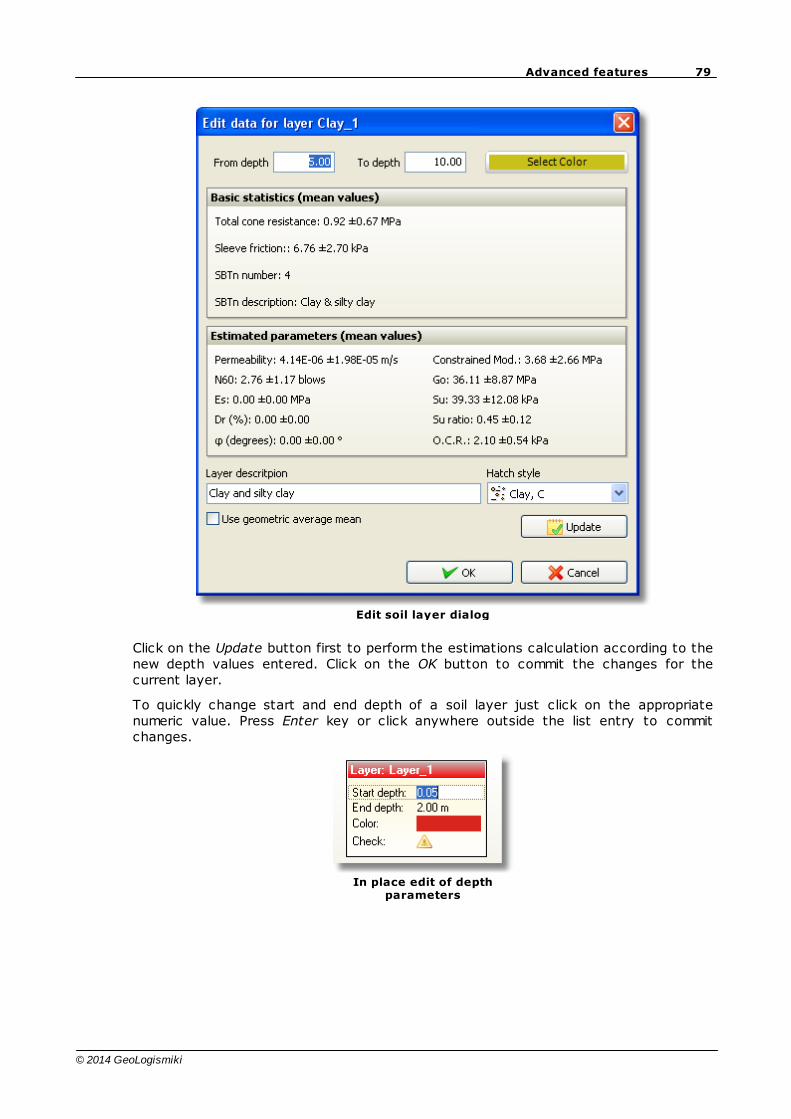
Edit soil layer dialog
Click on the Update button first to perform the estimations calculation according to thenew depth values entered. Click on the OK button to commit the changes for thecurrent layer.
To quickly change start and end depth of a soil layer just click on the appropriatenumeric value. Press Enter key or click anywhere outside the list entry to commitchanges.
In place edit of depthparameters
80 CPeT-IT User's Manual v.1.4
© 2014 GeoLogismiki
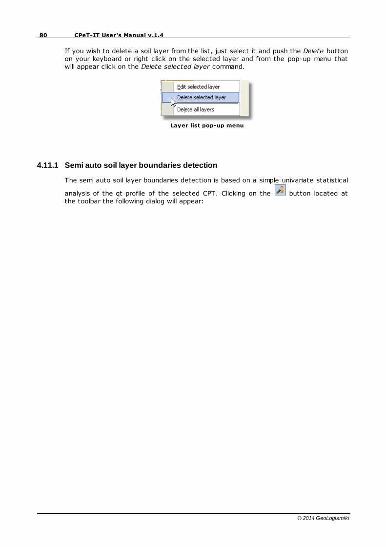
If you wish to delete a soil layer from the list, just select it and push the Delete buttonon your keyboard or right click on the selected layer and from the pop-up menu thatwill appear click on the Delete selected layer command.
Layer list pop-up menu
4.11.1 Semi auto soil layer boundaries detection
The semi auto soil layer boundaries detection is based on a simple univariate statistical
analysis of the qt profile of the selected CPT. Clicking on the button located atthe toolbar the following dialog will appear:
81Advanced features
© 2014 GeoLogismiki
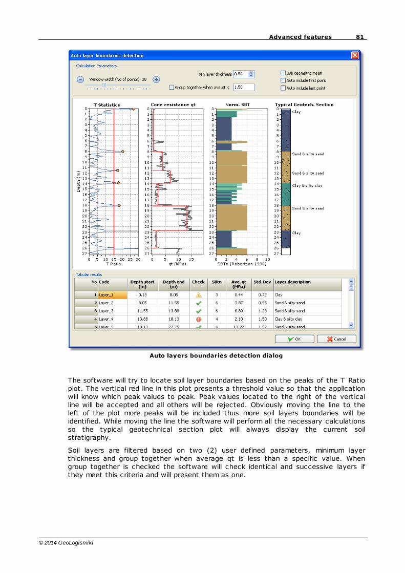
Auto layers boundaries detection dialog
The software will try to locate soil layer boundaries based on the peaks of the T Ratioplot. The vertical red line in this plot presents a threshold value so that the applicationwill know which peak values to peak. Peak values located to the right of the verticalline will be accepted and all others will be rejected. Obviously moving the line to theleft of the plot more peaks will be included thus more soil layers boundaries will beidentified. While moving the line the software will perform all the necessary calculationsso the typical geotechnical section plot will always display the current soilstratigraphy.
Soil layers are filtered based on two (2) user defined parameters, minimum layerthickness and group together when average qt is less than a specific value. Whengroup together is checked the software will check identical and successive layers ifthey meet this criteria and will present them as one.
82 CPeT-IT User's Manual v.1.4
© 2014 GeoLogismiki
The tabular results provide numeric results of the calculations along with a quick checkthat is based on the following rules:
When less than 5% of the CPT points that form a layer have a SBTn number outsidethe overall SBTn of the layer, then this layer is considered to be ok (a green tickmark appears on the Check column)
When 5% to 25% of the CPT points that form a layer have a SBTn number outsidethe overall SBTn of the layer, then this layer is considered to be less consistent (ayellow triangle mark appears on the Check column)
When more than 25% of the CPT points that form a layer have a SBTn numberoutside the overall SBTn of the layer, then this layer is not considered to be ok (ared circle mark appears on the Check column)
The Code column in the table is editable so the user can change the Code name ifneeded.
The statistical analysis is based on a window with a fixed width that moves from thetop of the CPT profile to the bottom. The width is calculated based on the number ofpoints (a default value of 30 is used) that can be changed using the track bar. Largenumber of points mean a smoother T Ratio plot, so less peaks will be displayed whereless points result to a large number of peaks.
Clicking the OK button the software will ask if it should replace any previousgeotechnical section with the current one. The user may review and make anychanges using the manual geotechnical section design module at any time.
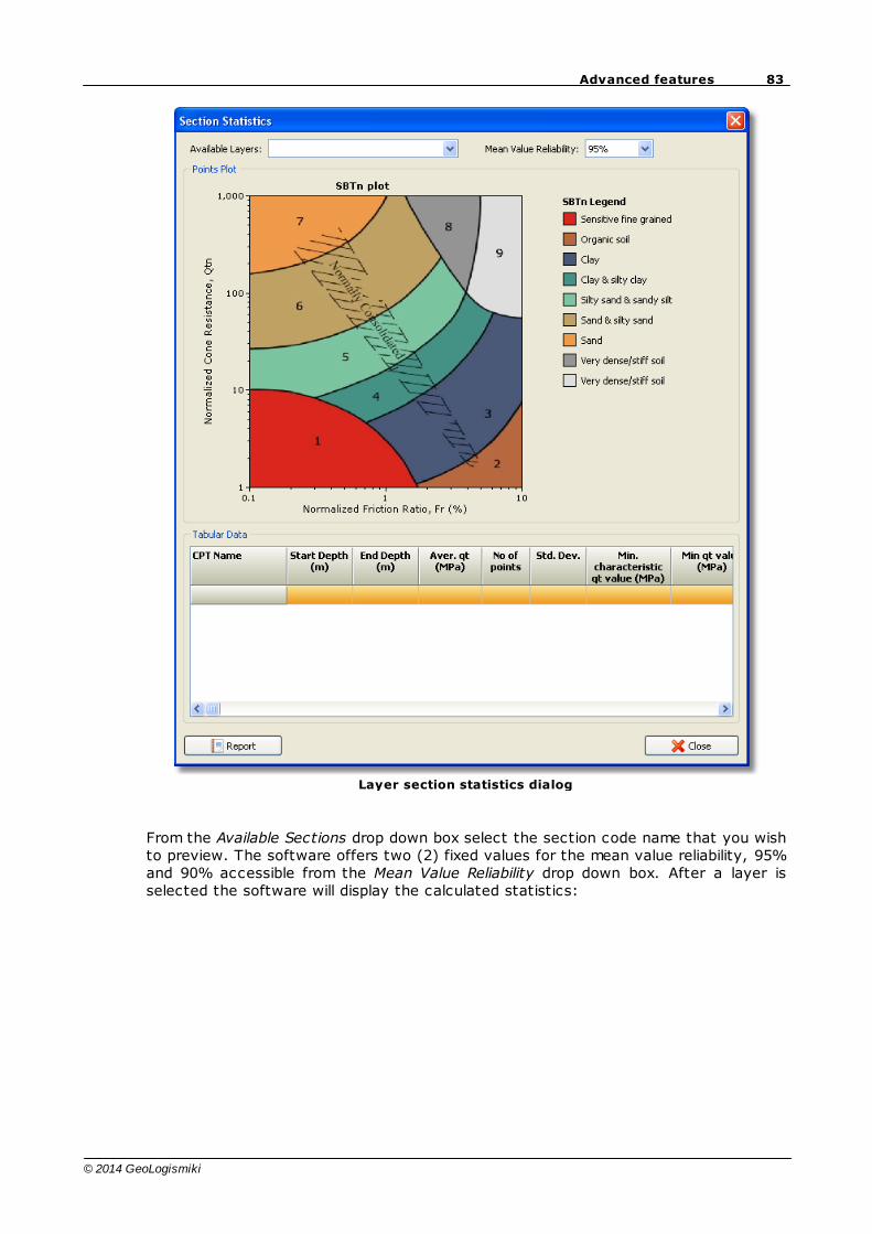
4.11.2 Geotechnical section layers statistics
Layers defined using the geotechnical section module may appear in several CPT filesin a single project file. The user may review the statistical properties of each layer interms of minimum characteristic values by clicking on the section statistics tool
button . The following dialog appears:
83Advanced features
© 2014 GeoLogismiki
Layer section statistics dialog
From the Available Sections drop down box select the section code name that you wishto preview. The software offers two (2) fixed values for the mean value reliability, 95%and 90% accessible from the Mean Value Reliability drop down box. After a layer isselected the software will display the calculated statistics:
84 CPeT-IT User's Manual v.1.4
© 2014 GeoLogismiki
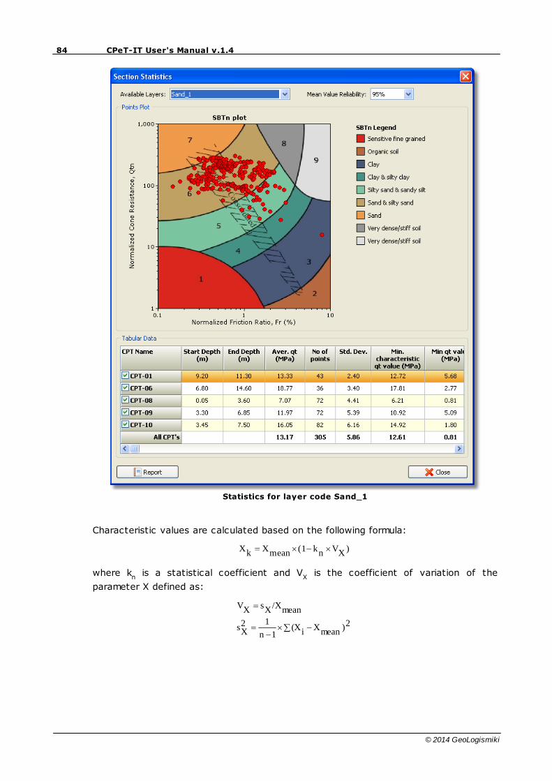
Statistics for layer code Sand_1
Characteristic values are calculated based on the following formula:
)XVnk(1meanXkX
where kn
is a statistical coefficient and VX
is the coefficient of variation of the
parameter X defined as:
2)meanXi(X1n
12Xs
mean/XXsXV
85Advanced features
© 2014 GeoLogismiki
where sX is the standard deviation of the n sample test.
4.12 Exporting data
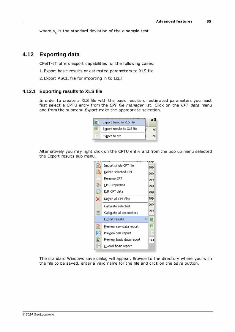
CPeIT-IT offers export capabilities for the following cases:
1. Export basic results or estimated parameters to XLS file
2. Export ASCII file for importing in to LiqIT
4.12.1 Exporting results to XLS file
In order to create a XLS file with the basic results or estimated parameters you mustfirst select a CPTU entry from the CPT file manager list. Click on the CPT data menuand from the submenu Export make the appropriate selection.
Alternatively you may right click on the CPTU entry and from the pop up menu selectedthe Export results sub menu.
The standard Windows save dialog will appear. Browse to the directory where you wishthe file to be saved, enter a valid name for the file and click on the Save button.
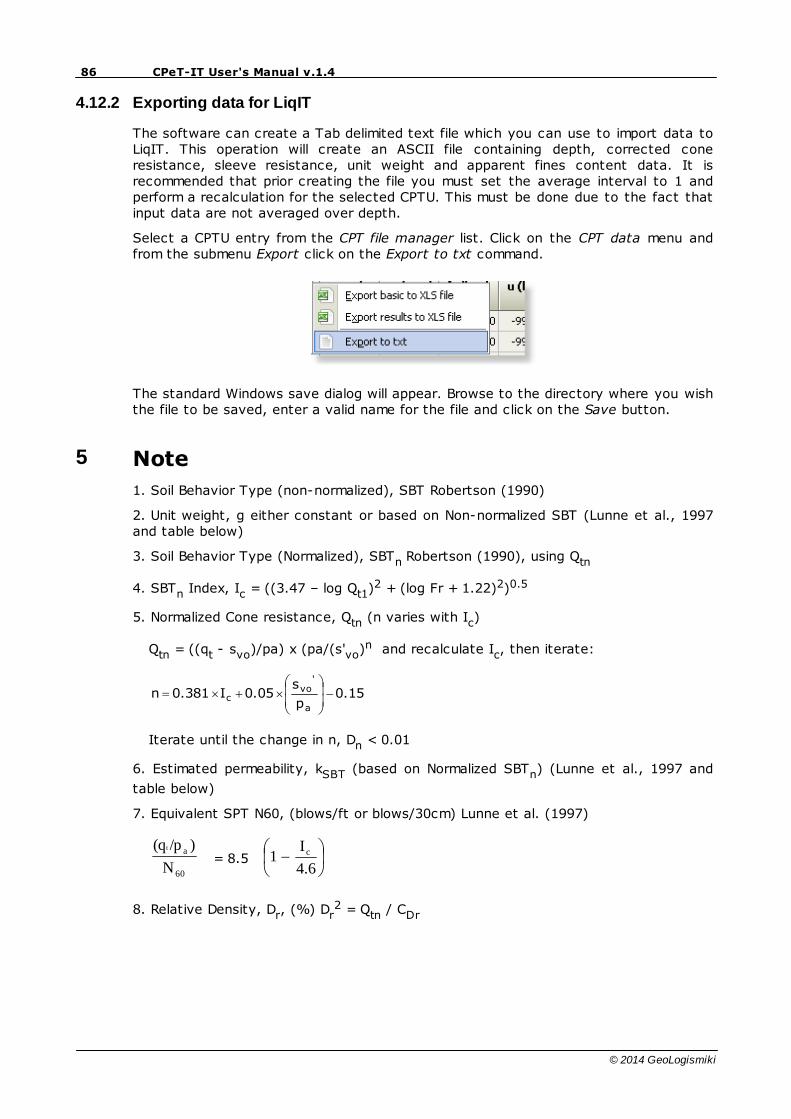
86 CPeT-IT User's Manual v.1.4
© 2014 GeoLogismiki
4.12.2 Exporting data for LiqIT
The software can create a Tab delimited text file which you can use to import data toLiqIT. This operation will create an ASCII file containing depth, corrected coneresistance, sleeve resistance, unit weight and apparent fines content data. It isrecommended that prior creating the file you must set the average interval to 1 andperform a recalculation for the selected CPTU. This must be done due to the fact thatinput data are not averaged over depth.
Select a CPTU entry from the CPT file manager list. Click on the CPT data menu andfrom the submenu Export click on the Export to txt command.
The standard Windows save dialog will appear. Browse to the directory where you wishthe file to be saved, enter a valid name for the file and click on the Save button.
5 Note
1. Soil Behavior Type (non-normalized), SBT Robertson (1990)
2. Unit weight, g either constant or based on Non-normalized SBT (Lunne et al., 1997and table below)
3. Soil Behavior Type (Normalized), SBTn Robertson (1990), using Qtn
4. SBTn Index, Ic = ((3.47 – log Qt1)2 + (log Fr + 1.22)2)0.5
5. Normalized Cone resistance, Qtn (n varies with Ic)
Qtn = ((qt - svo)/pa) x (pa/(s'vo)n and recalculate Ic, then iterate:
0.15p
s0.05I0.381n
a
'vo
c
Iterate until the change in n, Dn < 0.01
6. Estimated permeability, kSBT (based on Normalized SBTn) (Lunne et al., 1997 and
table below)
7. Equivalent SPT N60, (blows/ft or blows/30cm) Lunne et al. (1997)
60
a
N
)/p(qt
= 8.5 4.6
I1 c
8. Relative Density, Dr, (%) Dr2 = Qtn / CDr
87Note
© 2014 GeoLogismiki
Only SBTn 5, 6, 7 & 8 ‘0’ in zones 1, 2, 3, 4 & 9
9. Friction Angle, f', (degrees)
tQlog11 17.60 φ
Only SBTn 5, 6, 7 & 8 ’0’ in zones 1, 2, 3, 4 & 9
10. Young’s modulus, Es
1.68I0.55E
votEs
c100.015
sqE
Only when Ic < 2.60
11. Constrained Modulus, M
1.68I0.55M
c
tM
ttM
c
votM
c100.0188α
:use 2.20I When
14Q when 14α
14Q when Qα
:use 2.20I When
sqαM
12. Undrained shear strength, su = (qt - svo) / Nkt
Only SBTn 1, 2, 3, 4 & 9 ‘0’ in zones 5, 6, 7 & 8
13. Over Consolidation ratio, OCR = kocr Qt1
Only SBTn 1, 2, 3, 4 & 9 ‘0’ in zones 5, 6, 7 & 8
14. Small strain shear modulus, Go
1.68I0.55M
votM
c100.0188
sqG0
The following updated and simplified SBT descriptions have been used in the software:
SBT Zones SBTn Zones
1 sensitive fine grained 1 sensitive fine grained
2 organic soil 2 organic soil
3 clay 3 clay
4 clay & silty clay 4 clay & silty clay
5 clay & silty clay
6 sandy silt & clayey silt
7 silty sand & sandy silt 5 silty sand & sandy silt
88 CPeT-IT User's Manual v.1.4
© 2014 GeoLogismiki
8 sand & silty sand 6 sand & silty sand
9 sand
10 sand 7 sand
11 very dense/stiff soil* 8 very dense/stiff soil*
12 very dense/stiff soil* 9 very dense/stiff soil*
* heavily overconsolidated and/or cemented
Estimated Permeability (see Lunne et al., 1997)
SBTn Permeability (ft/sec) (m/sec)
1 3 x 10⁻⁸ 1 x 10⁻⁸
2 3 x 10⁻⁷ 1 x 10⁻⁷
3 1 x 10⁻⁹ 3 x 10⁻¹⁰
4 3 x 10⁻⁸ 1 x 10⁻⁸
5 3 x 10⁻⁶ 1 x 10⁻⁶
6 3 x 10⁻⁴ 1 x 10⁻⁴
7 3 x 10⁻² 1 x 10⁻²
8 3 x 10⁻⁶ 1 x 10⁻⁶
9 1 x 10⁻⁸ 3 x 10⁻⁹
Estimated Unit Weight (see Lunne et al., 1997)
SBT Approximate Unit Weight(lb/ft³)
(kN/m³)
1 111.4 17.5
2 79.6 12.5
3 111.4 17.5
4 114.6 18.0
5 114.6 18.0
6 114.6 18.0
7 117.8 18.5
8 120.9 19.0
9 124.1 19.5
10 127.3 20.0
89Note
© 2014 GeoLogismiki
11 130.5 20.5
12 120.9 19.0
6 LCPC method
The following text was taken from "Guide to cone penetration testing" by P. K.Robertson and K. L. Robertson. You may obtain a copy of the guide if you visit Dr.Robertson's personal web site at www.cpt-robertson.com or you may contact usdirectly and we will send you a copy.
Research has shown (Robertson et al., 1988; Briaud and Tucker, 1988; Tand andFunegard, 1989; Sharp et al., 1988) that CPT methods generally give superiorpredictions of axial pile capacity compared to most conventional methods. The mainreason for this is that the CPT provides a continuous profile of soil response. Almost allCPT methods use reduction factors to measured CPT values. The need for suchreduction factors is due to a combination of the following influences: scale effect, rateof loading effects, difference of insertion technique, position of the CPT friction sleeveand differences in horizontal soil displacements. The early work by DeBeer (1963)identified the importance of scale effects. Despite these differences, the CPT is stillthe test that gives the closest simulation to a pile. Superiority of CPT methods overnon CPT methods has been confirmed in other studies (e.g. O'Neill, 1986). The mainCPT method by Bustamante and Gianeselli (1982 - LCPC Method) is outlined below. TheLCPC CPT method is recommended since it provides simple guidance to account fordifferent pile installation methods and provides good estimates of axial capacity ofsingle piles.
The method by Bustamante and Gianeselli was based on the analysis of 197 pile load(and extraction) tests with a wide range of foundation and soil types, which maypartly explain the good results obtained with the method. The method, also known asthe LCPC method, is summarized in the following figures.
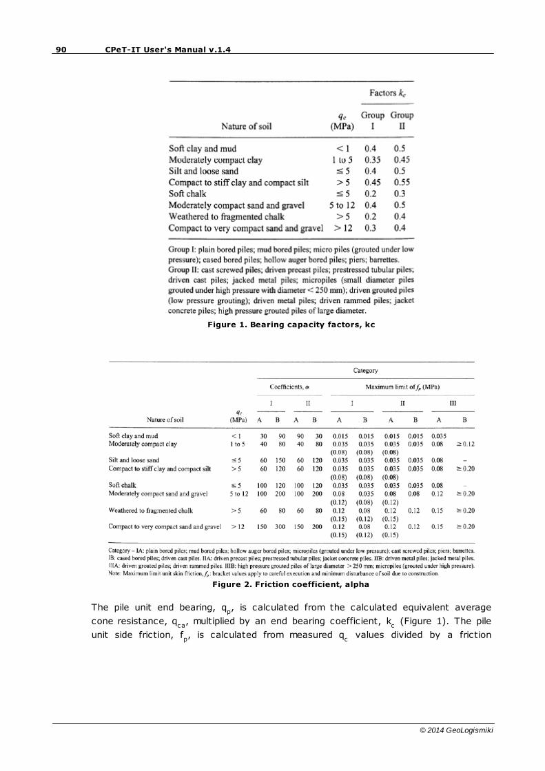
90 CPeT-IT User's Manual v.1.4
© 2014 GeoLogismiki
Figure 1. Bearing capacity factors, kc
Figure 2. Friction coefficient, alpha
The pile unit end bearing, qp, is calculated from the calculated equivalent average
cone resistance, qca
, multiplied by an end bearing coefficient, kc (Figure 1). The pile
unit side friction, fp, is calculated from measured q
c values divided by a friction
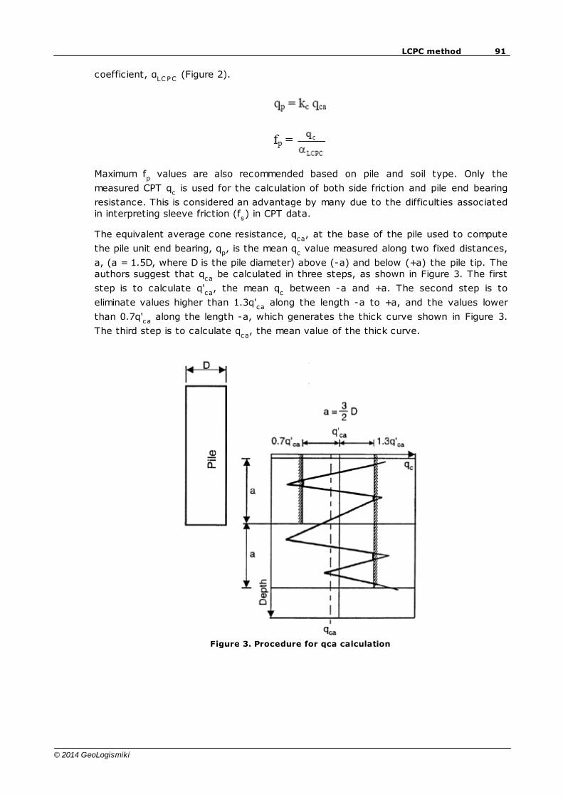
91LCPC method
© 2014 GeoLogismiki
coefficient, αLC PC
(Figure 2).
Maximum fp
values are also recommended based on pile and soil type. Only the
measured CPT qc is used for the calculation of both side friction and pile end bearing
resistance. This is considered an advantage by many due to the difficulties associatedin interpreting sleeve friction (f
s) in CPT data.
The equivalent average cone resistance, qca
, at the base of the pile used to compute
the pile unit end bearing, qp, is the mean q
c value measured along two fixed distances,
a, (a = 1.5D, where D is the pile diameter) above (-a) and below (+a) the pile tip. Theauthors suggest that q
ca be calculated in three steps, as shown in Figure 3. The first
step is to calculate q'ca
, the mean qc between -a and +a. The second step is to
eliminate values higher than 1.3q'ca
along the length -a to +a, and the values lower
than 0.7q'ca
along the length -a, which generates the thick curve shown in Figure 3.
The third step is to calculate qca
, the mean value of the thick curve.
Figure 3. Procedure for qca calculation

92 CPeT-IT User's Manual v.1.4
© 2014 GeoLogismiki
7 References
T. Lunne, P.K. Robertson and J.J.M. Powell, Cone Penetration testing in GeotechnicalPractice, 1997
Robertson, P.K., 2008, Guide to Cone Penetration Testing for GeotechnicalEngineering
Robertson, P.K., 2009, Interpretation of Cone Penetration Tests - a unifiedapproach., Canadian Geotechnical Journal (in press)
Designers' Guide to EN 1997-1, Eurocode 7: Geotechnical design - General rules, RFrank, C Bauduin, R Driscoll, M Kavvadas, N Krebs Ovesen, T Orr and B Schuppener

Back Cover