1

Abstract— Companies operating large data centers are focusing on how to reduce the electrical energy costs of operating data centers 24-7. A common way of reducing this cost is to perform dynamic voltage and frequency scaling (DVFS), thereby matching the CPU’s performance and power level to the incoming workload. Another power saving technique is CPU consolidation, which uses the minimum number of CPUs necessary to meet the service request demands and turns off the remaining idle CPUs. A key question that must be answered is which of these two techniques is more effective and under what conditions. This is the question that is addressed in this report. After analyzing the power consumption in a modern server system and developing appropriate power and performance models for the same, this report provides an extensive set of hardware-based experimental results and makes suggestions about how to maximize energy savings through CPU consolidation and/or DVFS. In addition, the report also presents new online CPU consolidation algorithms. The proposed algorithms reduce the energy delay product more than the Linux default DVFS algorithm (up to 13 %).

Index Terms—Algorithm, consolidation, energy efficiency, and

virtualization

I. INTRODUCTION ATA centers consist of a very large number of server machines that can be leased to provide cloud services to a

whole slew of clients running many different applications. The number of servers employed in data centers has been rapidly increasing, confirmed by the continuous increase in the BLADE server shipments in US and worldwide. Although the energy efficiency of server machines has been improving, this efficiency advances have not kept pace with the increase in cloud computing services and the concomitant increase in the number and size of data centers. As a result, an ever increasing amount of electrical energy is being consumed in today’s data centers, giving rise to concerns about the carbon emission footprint of data centers and the costs of operating them. The latter is especially important concern from the viewpoint of datacenter owners and operators (as well as their customers/clients who must eventually pay the bill).

Two widely accepted and employed techniques for increasing the power efficiency in data centers are server

This research is sponsored in part by a grant from the Semiconductor Research Corporation (No. 2012-HJ-2292).

I. Hwang and M. Pedram are with the Department of Electrical Engineering, University of Southern California, Los Angeles, CA 90036 USA (e-mail: inkwonhw@usc.edu; pedram@usc.edu).

consolidation and DVFS. The former aims at minimizing the number of active servers in a datacenter by consolidating all the incoming jobs into as few server machines as possible whereas the latter attempts to match the performance of each active server to the assigned workload to it so that energy can be saved at the level of each server. Server consolidation is needed and complements DVFS technique because of the energy no-proportional behavior of modern servers [1], and an unfortunate effect by which a server machine operating at a low performance level tends to consume power close to the power it consumes at its peak performance level. This is somewhat natural and expected because an electronic circuit (with server being a special case) consumes static power (leakage in CMOS digital circuits) regardless of whether it provides any computational services. The issue is, however, worse than simple leakage and has to do with the fact that many components within a modern server system (e.g., “uncore” logic within the processor chip, DRAM modules on the board, many of the I/O controllers, and even the network interface) cannot be scaled/modulated to exhibit a linear relationship between their power consumption and delivered performance levels.

A data center is typically under-utilized—by design, it has been designed to provide the required performance and satisfy its service level agreements (SLAs) with clients even during peak workload hours, and hence, at other times its resources are vastly under-utilized). For example, the minimum and the maximum utilization of the statically provisioned capacity of Facebook’s data center are 40% and 90%, respectively [2]. Hence, in light of the energy non-proportionality of today’s server base, a greater amount of energy costs can be reduced by consolidating jobs into as few server machines as possible and turning off the unused machines. The server consolidation has been studied very well, and many studies have suggested the use of virtual machine migration (VMM) as a means of doing server consolidation [3-7].

Although server consolidations can greatly lower a data center’s total energy consumption, there is still room for further energy savings due to the limitations and overheads associated with the server consolidation. For one, it is difficult to conduct server consolidation very frequently because the migration of tasks or virtual machines causes high overheads; e.g., heavy network traffic, high network latency and large system boot time, plus large energy consumption to move virtual machines and their local contexts around. Because of these overheads,

CPU Consolidation versus Dynamic Voltage and Frequency Scaling in a Virtualized Multi-Core

Server: Which is More Effective and When Inkwon Hwang, Student Member and Massoud Pedram, Fellow, IEEE

D

2

there is a relatively long period between server consolidation decision times. To avoid the SLA violations during each timing period when virtual machine to server assignments are fixed, virtual machines (or tasks) are not too tightly consolidated into active server set in order to provide a safe margin of operation (too aggressive a consolidation strategy will result in violation of client SLAs and the characteristic need to compensate the clients for missing their agree upon performance targets). The longer the period is, the larger the margin becomes (i.e., more server machines are utilized). Hence, the server machines are still under-utilized, which implies that there is the potential of the further energy savings through additional resource management techniques.

There are a number of resources in a computer system (computing, storage, I/ bandwidth). This study focuses on the computing resource, i.e., the CPU, which is a major energy consumer. A well-known and common energy-aware CPU management technique is a Dynamic Voltage and Frequency Scaling (DVFS) [3, 8, 9]. The DVFS was introduced decades ago, and it has been one of the most effective power saving techniques for CPUs. The amount of the energy savings by DVFS, however, is decreasing due to the following reasons. First, the supply voltages have already become quite low (sub-one volt) and hence the remaining headroom for further supply voltage reductions is small and shrinking. Second, many modern servers have two or more processor chips, each chip containing multiple CPUs (cores1) but a single on-chip power distribution network shared by all the CPUs. Because of this sharing, the CPUs on the same chip must operate at the same supply voltage level and hence the same clock frequencies2. In other words, we cannot set different frequencies for individual CPUs, which means that, unless we do ‘perfect’ load balancing among CPUs sharing the same power bus, the voltage level that is set for the most highly loaded CPU will result in a number of under-utilized CPUs where the available performance level is higher than what is actually needed, hence energy is wasted. Third, in a virtualized server system, it is difficult to gather sufficient information about the running applications, which is necessary to choose the optimal clock frequency and voltage level for the CPUs. This is because the virtual machine manager (hypervisor), which conducts DVFS, resides in a privileged domain whereas the applications are running in a different domain (virtual machine domain) [4].

Another well-known CPU energy management technique is Dynamic Power State Switching. Many modern processors support multiple power states (known as C-States). Each C-state specifies the processor modules which are turned ON or OFF. Based on the recent workload intensity of the CPU, the operating system (OS) decides the power state of each CPU. Note that the power state of each CPU may be different from that of another CPU (even when the two CPUs are on the same processor). This is because each CPU is placed in its own power domain on the processor, and the power to each such domain can be independently gated. The OS can suggest a

1 The terms ‘CPU’ and ‘core’ are used interchangeably in this paper. 2 Some processors are capable of independent DVFS among cores while

Intel processors are not. This study targets Intel processors.

power state of a CPU, but the final decision is made by a Power Control Unit (PCU) which resides in the processor chip. This is because the suggestion from the OS may not be a good one. For example, it may result in too frequent power state changes or too quick a transition to a sleep state.

The PCU also decides about the power states of some of the other modules on the processor chip by using its fine-tuned algorithms. We believe that the PCU can save more energy if there is software-level assistance for it. In this study, we present a CPU consolidation technique, which helps the PCU achieve more energy savings. This technique explicitly defines sets of active and inactive (sleep) CPUs, and ensures lower performance degradation and energy waste by avoiding unnecessary power state switches.

There have been many research studies that investigate the effectiveness of the CPU consolidation. In [10] the authors show that consolidation across CPUs in a single processor and two processor systems offers a very small amount of energy savings. They used their own benchmark which is not the standard and may not create realistic workloads. In [11] Jacob et al. compare core-level power gating (CPG) with DVFS and show that CPG saves more energy by 30% than DVFS. This result implies the energy savings by the CPU consolidation may be larger if the processor supports the CPG. However, the reported results are calculated from a combination of real measurements and estimated leakage power values (the adopted leakage power model is somewhat simple). In [2] the authors present a technique called core count management (CCM), which is a variant of the CPU consolidation technique, and report 35% energy savings. However, all results are obtained using a simulator, and the power and performance models used in the simulator are again fairly simplistic.

This report is differentiated from the prior work because of the following reasons. First, all results are obtained from the actual hardware measurements and not simulations. Second, realistic workloads based on SPEC benchmark suite have been used. Third, this report investigates the relative effectiveness of CPU consolidation vs. DVFS as means of power savings in multi-core/processor server systems.

A preliminary version of this work has been published in [12]. This technical report is a substantially extended version, which includes a completely new power model, vastly more detailed experimental results and discussions, and a more efficient online CPU consolidation algorithm.

The remainder of the report is organized as follows. Several mechanisms of CPU power management are reviewed in Section II. In Section III we present the power and latency models, which enable us to show how the CPU consolidation affects the power and latency of a system. A detailed description of the experimental system setup is provided in Section IV. Section V presents our detailed experimental results and discussions. Finally, we summarize the results and provide some useful conclusions and insights in Section VI.

3

II. BACKGROUND – POWER MANAGEMENT TECHNOLOGIES Most of modern operating systems (OS) reduce the power

consumption of a processor by dynamically changing a power state of the processor. In order to change this state, an OS requires appropriate interfaces to communicate with the processor. For this purpose the Advanced Configuration and Power Interface (ACPI) specification was developed as an open standard for OS-directed power management. This specification is a processor-independent standard; hence an OS is capable of controlling power state of any processors. In this section, the processor power and performance states as well as OS-directed power management mechanism are briefly reviewed.

A. Processor power states (C-States) The ACPI specification defines C-States, which are also

known as ‘sleep states’. When a processor is in a higher-numbered C-State, which is also called a ‘deeper’ sleep state, a larger number of internal modules of the processor are turned off. The processor, therefore, consumes lower power in a deeper state. However, it also takes longer time for the processor to go back to a fully active state (i.e., C0 state) starting from a deeper sleep state. The number of supported C-States is processor-dependent; e.g., the Intel® Core™ i7 processor (code-named Nehalem) supports C0, C1/C1E, C3, and C6 states.

There are two types of C-States: core and processor. These core C-state (𝐶𝐶𝑛) and processor C-state (𝑃𝐶𝑛) are hardware C-states. The CC-state of a core may be different from that of others. The PC-state is related to the CC-States. In particular, when all cores are in the same CC-State, the processor transitions into the corresponding PC-state. This is reasonable because of all the processor resources that are shared by the cores. For example, the Intel i7 processor’s L2 cache is shared by four cores, so the processor cannot make a transition to a deep PC-State when any of the cores are still active. Otherwise, the shared L2 cache may become inactive, which would prohibit the active cores from proper functioning.

In addition to these hardware C-states, there is the notion of logical C-States (𝐶𝑛). An OS ‘requests’ a change in C-State of logical cores 3, but the request may be denied (called auto demotion). The decision of demotion is made based on each core’s immediate residency history; if the transition rate of C-States is too high, the request for a transition can be ignored. In general, the entry/exit costs (latency and energy overheads) increase when the processor/core escapes from a deeper state; hence, the auto demotion prevents unnecessary excursions into deeper power states, and thereby, reduces both latency and energy overheads.

B. Processor performance state (P-States) Each power state (P-State) specifies the clock frequency and

voltage of the cores (i.e., the voltage/frequency setting). At the higher clock frequency, the performance of a core is higher. Similar to the C-States, the number of supported P-States is

3 A logical core is identical to a physical core unless Intel hyper-threading is enabled. In this study hyper-threading was disabled.

processor-dependent. A clock frequency of a core is higher at lower numbered P-States; e.g., P0 is the highest performance state.

An OS decides which P-State is more appropriate for a core and changes the state. This decision is made based on the historical workload information. The OS may not choose the same state for all cores, but all cores in the Intel processors will run at the same clock frequency because the clock generator module is shared by all these cores. Therefore, even if the OS sets different P-States for the cores, only one state is selected and applied to all the cores. In general, the highest performance state of any core is selected and used as the P-state for all cores, but another decision policy may be used. Because of this hardware constraint of the current Intel processors, it is recommended to distribute the workload evenly among all active cores. Otherwise, the selected P-State will be appropriate only for some cores, but not for the others.

C. Core-level power gating Recent state-of-the-art Intel processors are capable of

core-level power gating, that is, processors can completely shut down some of the cores (the OFF cores consume nearly zero power). Processors with the power gating feature thus have an additional C-State (C7) corresponding to near zero power dissipation, but with the largest entry/exit costs. Note that the processor used in this study supports core-level power gating.

III. POWER AND LATENCY MODELS In this section we present power and latency models for the

target server system. Based on these models, we will investigate how the CPU consolidation affects the power dissipation and latency of the server. From now on, the CPU consolidation is simply called ‘consolidation’. From the analysis we will derive insights about how the consolidation affects the power dissipation and latency. The analysis about the power/latency tradeoffs will be verified by empirical results in a later section. Note that thermal issues (e.g., leakage power variation as a function of chip temperature) are not considered. This is because we can do consolidation only when the system is under-utilized, which also implies that the temperature of processor chips is not so high.

A. Power model This section presents a full platform-level power dissipation

model, accounting for the power consumed by all components within a modern multi-processor server system. This power model estimates the system power dissipation by using statistical data reported by the system itself; i.e., the percentage of time spent in specific core/processor C-state.

The processor power dissipation consists of core and uncore power dissipations. The core includes all circuits used to perform arithmetic/logic operations and L1 cache memories whereas the term uncore refers to all other components in a processor. Next we provide some notation and their definitions.

• 𝑃𝑎𝑐𝑡𝑖𝑣𝑒𝑐𝑜𝑟𝑒 – Power dissipation by a core when the core is active (i.e., executing tasks)

4

• 𝑃𝐶𝐶𝑛𝑐𝑜𝑟𝑒 – Power dissipation by a core when it is in the core

C-state n (𝐶𝐶𝑛), i.e., the core is in some sleep state. Note that 𝑃𝐶𝐶0𝑐𝑜𝑟𝑒 is different from 𝑃𝑎𝑐𝑡𝑖𝑣𝑒𝑐𝑜𝑟𝑒 .

• 𝑃𝑃𝐶𝑛𝑢𝑛𝑐𝑜𝑟𝑒 – Power dissipation by uncore when the processor is

in processor C-state n (𝑃𝐶𝑛). • 𝑇𝑎𝑐𝑡𝑖𝑣𝑒

𝑐𝑜𝑟𝑒𝑖 – Percentage of time when a core is active and executing tasks, which is also called (core) utilization (Utili).

• 𝑇𝐶𝐶𝑛𝑐𝑜𝑟𝑒𝑖 – Percentage of time when a core is in the 𝐶𝐶𝑛 state.

• 𝑇𝑃𝐶𝑛𝑢𝑛𝑐𝑜𝑟𝑒 – Percentage of time spent by the processor in the

𝑃𝐶𝑛 state.

Total (server platform) power dissipation is the sum of the processor power dissipation and the power consumed by other components, e.g., I/O, memory, and hard disc drive (HDD):

icoretotal uncore otheriP P P P= + +∑ (1)

The core power dissipation can be estimated using 𝑃𝑎𝑐𝑡𝑖𝑣𝑒𝑐𝑜𝑟𝑒 , 𝑃𝐶𝐶𝑛𝑐𝑜𝑟𝑒, 𝑇𝑎𝑐𝑡𝑖𝑣𝑒

𝑐𝑜𝑟𝑒𝑖 , and 𝑇𝐶𝐶𝑛𝑐𝑜𝑟𝑒𝑖 as shown below. CC0 is a special state;

a core is in the CC0 state when the core is normal operating state (i.e., executing tasks). Note, however, that the CPU stays in that state for a certain time (i.e., a timeout period) even when the core becomes idle.

( )

( )

0 0

0

1

0

i i ii

in n

i in n

core core corecore core coreactive active CC activeCC

corecoreCC CCn

core corecore core coreactive CC active CC CCn

P P T P T T

P T

P P T P T

≥

≥

= ⋅ + ⋅ −

+ ⋅

= − ⋅ + ⋅

∑∑

(2)

Similar to the core power dissipation, the uncore power dissipation is:

n n

uncore uncore uncorePC PCnP P T= ⋅∑ (3)

Let us say we want to reduce the active CPU count (i.e., perform CPU consolidation). The workload level does not change, so the power dissipations by other parts of the server (𝑃𝑜𝑡ℎ𝑒𝑟) are not affected. In addition, the percentage of time spent in the 𝑃𝐶𝑛 state (𝑇𝑃𝐶𝑛

𝑢𝑛𝑐𝑜𝑟𝑒 ) is only a function of the workload level of the processor. In other words, changing the active CPU count does not affect 𝑃𝑢𝑛𝑐𝑜𝑟𝑒 when the workload level does not change. Therefore, the amount of change in power dissipation as a result of CPU consolidation is:

( ) ( )0 0

i

i i

n n

coretotali

core corecore core coreactive CC active CC CCi n i

P P

P P T P T≥

∆ = ∆

= − ∆ + ∆

∑∑ ∑ ∑

(4)

In the above equation, the sum of 𝑇𝑎𝑐𝑡𝑖𝑣𝑒𝑐𝑜𝑟𝑒𝑖 is not affected by the

consolidation because the workload load level does not change; that is, 0icore

activeiT∆ =∑ . Therefore,

( )0i

n n

coretotal coreCC CCn i

P P T≥

∆ = ∆∑ ∑ (5)

As shown in the above equation, the power savings of consolidation is a function of changes in 𝑇𝐶𝐶𝑛

𝑐𝑜𝑟𝑒𝑖 . CPU consolidation makes inactive CPUs go to the deepest CC state, which can reduce power dissipation. However, at the same time, it also forces the active CPUs to stay in deeper CC states for less amount of time because the utilization level of these active CPUs increases. This may increase overall power dissipation.

The percentage of time spent in the 𝐶𝐶𝑛 state (𝑇𝐶𝐶𝑛𝑐𝑜𝑟𝑒𝑖) is

influenced by many factors, and some of these factors are unknown, e.g., details of the algorithm responsible for changing the core C-states. Therefore, we will quantify the power savings of CPU consolidation based on experimental results.

B. Latency (delay) model The proposed latency model is a function of its utilization

level, which is denoted by 𝑇𝑎𝑐𝑡𝑖𝑣𝑒𝑐𝑜𝑟𝑒𝑖 . In general, the latency

rapidly increases when a CPU approaches full utilization [5]:

1 i

i coreactive

eL fT

= +−

(6)

where 𝐿𝑖 is the latency of the 𝑖th CPU. The proposed latency model must have another term that causes the latency to reduce at higher utilization levels. This is because at higher utilization there will be less frequent C-State transitions. Recall that although switching to a deeper sleep state saves power, it takes additional time to escape from a deeper sleep state. Therefore, we have:

1

i

i

corei activecore

active

eL f gTT

= + − −

(7)

The latency is affected by CPU consolidation because 𝑇𝑎𝑐𝑡𝑖𝑣𝑒𝑐𝑜𝑟𝑒𝑖 is a function of the active CPU count. When 𝐾 tasks are

assigned to the system every second, the tasks are evenly distributed to the 𝑚 active CPUs by a scheduler. Each CPU thus serves 𝐾/𝑚 tasks every second. It is reasonable to suppose 𝑇𝑎𝑐𝑡𝑖𝑣𝑒𝑐𝑜𝑟𝑒𝑖 is linearly proportional to the workload (𝐾/𝑚): ( )icore

activeT d K m= (8) However, this statement may not be valid when the workload is very high. As an example, consider a scenario whereby 𝐻 = 𝐾/𝑚 memory-bound tasks are sent to the target CPU every second. If more tasks (say 2 × 𝐻) are sent to the target CPU per second, the cache miss rate on that CPU will also increase (more precisely, the working sets of the 2 × 𝐻 tasks will not fit on the cache, and therefore, every task will experience a higher cache miss rate on average). This means that the execution time of the tasks increases, and therefore, the CPU utilization will increase super-linearly. Thus, the utilization equation may be written as follows:

2( ) ( )icoreactiveT c K m d K m= + (9)

Now we can write the latency as a function of the active CPU count (m) and the total number of tasks (K):

( ) ( )

( ) ( )221eL f gc K m gd K m

c K m d K m= + − −

− −(10)

The relationship between the coefficient ‘c’ and latency is shown in Fig. 1(a); the larger ‘c’ is, the larger the latency is. This makes sense because bigger overhead causes the latency to increase. Therefore, the consolidation may incur potentially high latency penalty if ‘c’ is large. The effect of another coefficient ‘g’ is shown in Fig. 1(b); the latency may decrease as fewer CPUs are used when ‘g’ is positive. However, as shown in Fig. 1(b), the latency increases rapidly at last when the

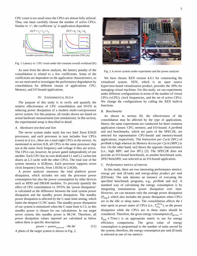
5

CPU count is too small since the CPUs are almost fully utilized. Thus, one must carefully choose the number of active CPUs. Similar to ‘c’, the coefficient ‘g’ is application-dependent.

Fig. 1 Latency vs. CPU count under the constant overall workload (K)

As seen from the above analysis, the latency penalty of the consolidation is related to a few coefficients. Some of the coefficients are dependent on the application characteristics, so we are motivated to investigate the performance degradation by consolidation for different classes of applications: CPU, Memory, and I/O bound applications.

IV. EXPERIMENTAL SETUP The purpose of this study is to verify and quantify the

relative effectiveness of CPU consolidation and DVFS in reducing power dissipation of a modern multi-core/processor server system. For this purpose, all results shown are based on actual hardware measurement (not simulations). In this section, the experimental setup is described in detail.

A. Hardware test-bed and Xen The server system under study has two Intel Xeon E5620

processors, and each processor in turn includes four CPUs (cores) in it (i.e., there are a total eight CPUs in the server). As mentioned in section II.B, all CPUs in the same processor chip run at the same clock frequency and voltage if they are active. The CPUs can, however, be power gated independently of one another. Each CPU has its own dedicated L1 and L2 caches but shares an L3 cache with the other CPUs. The total size of the system memory is 6GBytes. Each processor supports seven clock frequency levels, from 1.6GHz to 2.4GHz.

A power analyzer measures the total platform power dissipation, which includes not only the processor power consumption but also the power consumption by other devices such as HDD and DRAM modules. To precisely quantify the effect of CPU consolidation vs. DVFS, the ‘power dissipation’ is calculated as the difference between the total system power dissipation and the standby power dissipation. The standby power dissipation is affected by the C-state limit setting, which limits the deepest CC/PC states. The standby power dissipation of our system is minimized when the C-state limit is C3, so this standby power is chosen for our calculations. In our target server system, this standby power is 98.1W. Therefore, all power dissipation values reported are calculated as below unless there is specific description:

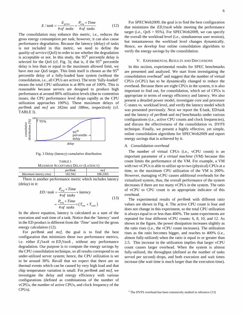
98.1measuredpower power W= − (11) A photo of the target system is shown in Fig. 2.

Fig. 2 A server system under experiment and the power analyzer

We have chosen XEN version 4.0.1 for constructing the virtualized system. XEN, which is an open source hypervisor-based virtualization product, provides the APIs for managing virtual machines. For this study, we ran experiments under different configurations in terms of the number of virtual CPUs (vCPU), clock frequencies, and the set of active CPUs. We change the configurations by calling the XEN built-in functions.

B. Benchmarks As shown in section III, the effectiveness of the

consolidation may be affected by the type of applications. Hence, the same experiments are conducted for three common application classes: CPU, memory, and I/O-bound. A perlbmk and mcf benchmarks, which are parts of the SPEC2K, are selected for representative CPU-bound and memory-bound applications, respectively. The Instruction per Cycle (IPC) of perlbmk is high whereas its Memory Access per Cycle (MPC) is low. On the other hand, mcf shows the opposite characteristics (i.e., high MPC and low IPC) [3]. The SPEC2K does not provide an I/O-bound benchmark, so another benchmark suite, SPECWeb2009, was selected as an I/O-bound application.

C. Performance metrics of interest In this study, there are two interesting performance metrics:

energy per task (E/task) and energy-delay product per task (ED/task). The task denotes an instance of executing the specified benchmark programs, e.g., perlbmk and mcf. A standard way of calculating the energy consumption is by integrating instantaneous power dissipation over time. However, we can measure only the average power dissipation (𝑃𝑎𝑣𝑔), which also includes the power dissipation when CPUs are in the idle or sleep states. The consolidation affects the f time spent in power states of CPUs (i.e., 𝑇𝐶𝐶𝑛

𝑐𝑜𝑟𝑒𝑖), so the power dissipation while the CPUs are in these states should be considered. Therefore, the gross energy consumption (𝐸𝑔𝑟𝑜𝑠𝑠 =𝑃𝑎𝑣𝑔 × 𝑇𝑖𝑚𝑒 ) is an appropriate metric to use for energy efficiency comparisons. The gross value of energy consumption is proportional to the number of tasks served by the system; therefore, the energy consumption per task (E/task) is selected as one of our metrics:

number of active CPUs (m)

late

ncy

(a) 0 < c1 < c2 < c3

number of active CPUs (m)

late

ncy

(b) 0 < g1 < g2 < g3

c1

c2

c3

g1

g2

g3

6

/# #

gross avgE P TimeE task

of tasks of tasks×

= = (12)

The consolidation may enhance this metric, i.e., reduces the gross energy consumption per task; however, it can also cause performance degradation. Because the latency (delay) of tasks is not included in this metric, we need to define the quality-of-service (QoS) in order to see whether the degradation is acceptable or not. In this study, the 95th percentile delay is selected for the QoS (cf. Fig. 3); that is, if the 95th percentile delay is less than or equal to the maximum allowed limit, we have met our QoS target. This limit itself is chosen as the 95th percentile delay of a fully-loaded base system (without the consolidation, i.e., all CPUs are active). The term ‘fully-loaded’ means the total CPU utilization is at 80% out of 100%. This is reasonable because servers are designed to produce high performance at around 80% utilization levels (due to contention issues, the CPU performance level drops rapidly as the CPU utilization approaches 100%). These maximum delays of perlbmk and mcf are 182ms and 188ms, respectively (cf. TABLE I).

Fig. 3 Delay (latency) cumulative distribution

TABLE I MAXIMUM ACCEPTABLE DELAY (LATENCY)

perlbmk mcf Maximum latency (ms) 182.942 188.2305 There is another performance metric which includes latency

(delay) in it:

( )

/#

#

avg

avgexe wait

P TimeED task latency

of tasksP Time

T Tof tasks

×= ×

×= × +

(13)

In the above equation, latency is calculated as a sum of the execution and wait time of a task. Notice that the ‘latency’ used in the ED product is different from the ‘Time’ used for the gross energy calculation (12).

For perlbmk and mcf, the goal is to find the best configuration that minimizes these two performance metrics, i.e. either 𝐸/𝑡𝑎𝑠𝑘 or 𝐸𝐷/𝑡𝑎𝑠𝑘 , without any performance degradation. Our purpose is to compute the energy savings by the CPU consolidation technique, so all results correspond to an under-utilized server system; hence, the CPU utilization is set to be around 30%. Recall that we expect that there are no thermal events which can be caused by very high load and that chip temperature variation is small. For perlbmk and mcf, we investigate the delay and energy efficiency with various configurations (defined as combinations of the number of vCPUs, the number of active CPUs, and clock frequency of the CPUs).

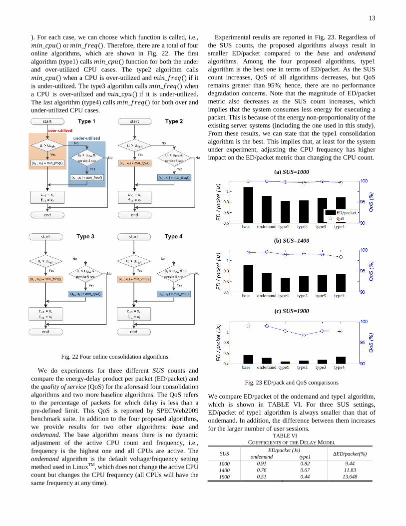
For SPECWeb2009, the goal is to find the best configuration that minimizes the 𝐸𝐷/𝑡𝑎𝑠𝑘 while meeting the performance target (i.e., QoS > 95%). For SPECWeb2009, we can specify the overall the workload level (i.e., simultaneous user session), but instantaneous the workload level changes dynamically. Hence, we develop four online consolidation algorithms to verify the energy savings by the consolidation.

V. EXPERIMENTAL RESULTS AND DISCUSSIONS In this section, experimental results for SPEC benchmarks

are presented and analyzed. We start from investigating the consolidation overhead4 and suggest that the number of virtual CPUs (vCPU) has to be dynamically changed to reduce the overhead. Because there are eight CPUs in the system, it is also important to find out, for consolidation, which set of CPUs is appropriate in terms of energy efficiency and latency. We also present a detailed power model, investigate core and processor C-states vs. workload level, and verify the latency model which was presented previously. Next we report the E/task, ED/task and the latency of perlbmk and mcf benchmarks under various configurations (i.e., active CPU counts and clock frequencies), and discuss the effectiveness of the consolidation vs. DVFS technique. Finally, we present a highly effective, yet simple, online consolidation algorithms for SPECWeb2009 and report energy savings that is achieved by it.

A. Consolidation overhead The number of virtual CPUs (i.e., vCPU count) is an

important parameter of a virtual machine (VM) because this count limits the performance of the VM. For example, a VM with two vCPUs is able to utilize up to two (physical) CPUs at a time, so the maximum CPU utilization of the VM is 200%. However, managing vCPU causes additional overheads for the virtualized system, thus, the overall performance of the system decreases if there are too many vCPUs in the system. The ratio of vCPU to CPU count is an appropriate indicator of this overhead.

The experimental results of perlbmk with different ratio values are shown in Fig. 4. The active CPU count is four and does not change in this experiment, so the total CPU utilization is always equal to or less than 400%. The same experiments are repeated for four different vCPU counts: 6, 8, 10, and 12. As shown in the figure, the power dissipation increases slightly as the ratio rises (i.e., the vCPU count increases). The utilization rises as the ratio becomes bigger, and reaches to 400% (i.e., almost fully-utilized) when the ratio is equal to or greater than 2.5. This increase in the utilization implies that larger vCPU count causes larger overhead. When the system is almost fully-utilized, the throughput (defined as the number of tasks served per second) drops, and both execution and wait times increase (the wait time is much larger than the execution time).

4 The DVFS overhead has been extensively studied in reference [13]

0

100

delay

cum

ulat

ive

dist

ribu

tion

(%)

↑ 95%

95thpercentile →delay

7

Fig. 4 Consolidation overhead – perlbmk

The results of mcf are reported in Fig. 5. The utilization increases slightly as the ratio becomes higher whereas the power and throughput are almost independent of the ratio. The wait time increases rapidly when the ratio is greater than four; that is, for mcf, the overheads of managing vCPUs are less than perlbmk. However, this does not mean that this overhead is negligible for mcf; the ratio has to be smaller than four to avoid significant performance degradation.

Fig. 5 Consolidation overhead – mcf

From the results reported above, it is important to adjust the vCPU count for both perlbmk and mcf. We keep the vCPU to CPU count ratio at around two for all test cases presented from now on.

B. Selecting CPUs for consolidation The basic idea of the consolidation is to utilize the minimum

number of CPUs; hence we can turn off as many CPUs as possible. In addition to the active CPU count, CPU selection scheme may be important for multi core/processor systems.

A naming convention for CPUs in the target server system is shown in Fig. 6. An ID starts from 0 and the biggest ID is 3. The ID of the second processor starts from 4. When two CPUs are selected from the eight CPUs, there are total 28 possible cases. However, by considering redundancy, only three meaningful cases are: ‘0, 1’, ‘0, 2’, and ‘0, 4’ cases. The first one (i.e., ‘0, 1’ case) selects the first two CPUs which are close to each other. The second case (‘0, 2’ case) chooses two CPUs from the same processor package, but there is another CPU between them. The last one (‘0, 4’ case) selects a CPU from each package. The comparisons among these three cases are shown in Fig. 7.

Fig. 6 CPU/core ID naming

The power and latency comparisons of perlbmk/mcf for three distinct sets of active CPUs are shown in Fig. 7. As shown in the figure, there is no noticeable difference among the three active CPU sets. It is because, as shown in Fig. 6, the architecture of the processor is symmetric; hence there is no difference between case ‘0, 1’ and ‘0, 2’. In addition, we can use only two active CPUs when the utilization is relatively low (up to 200% out of 800%); therefore, the difference in power dissipation and latency between two active CPU sets, even if it exists, may not significant. Therefore, if we need only two active CPUs (i.e., when the workload level is quite low), any set of CPUs can be selected.

Fig. 7 Power and delay vs. CPU IDs – 2 active CPUs

Now we do similar experiments for the other case that four CPUs are active. The three representative active CPU sets are selected for the experiments: ‘0, 1, 2, 3’, ‘0, 2, 4, 6’, and ‘0, 1, 4, 5’ cases. For the first case, all four CPUs are selected from one processor. The second case utilizes two CPUs from each processor. The third case looks similar to the second one except that two CPUs in the same processor reside next to each other.

The power and latency comparisons of perlbmk/mcf are shown in Fig. 8. Both power dissipation and utilization is smallest for the first case ‘0, 1, 2, 3’, which selects all CPUs from the same processor. However, the amount of difference is quite small. Notice that throughputs (i.e., tasks/s) of three sets of active CPUs are almost identical to one another. More noticeable difference is observed for latency; latency of the first case is smallest. It is because the overhead of context switch within a processor is less than that of context switch from a processor to another one. On the other hand, for mcf, all kinds of metrics are almost independent of active CPU sets.

8

Therefore, when we need four active CPUs, we can select all CPUs from the same processor regardless of characteristics of applications, i.e. either CPU or memory bound. It is because the selection method reduces both latency and power dissipation of CPU bound applications.

Fig. 8 Power and delay vs. CPU IDs – 4 active CPUs

Based on the experimental results shown above, we use a simple active CPU selection method, which is shown in TABLE II. This method may not be appropriate for the other processors, but a similar method as above can be used to derive similar tables for other processor systems.

TABLE II ACTIVE CPU SELECTION

CPU count CPU IDs CPU count CPU IDs 2 0, 1 5 0, 1, 2, 3, 4 3 0, 1, 2 6 0, 1, 2, 3, 4, 5 4 0, 1, 2, 3 7 0, 1, 2, 3, 4, 5, 6

C. Power model derivation and verification This section presents a full platform-level power dissipation

model, accounting for the power consumed by the core and uncore components within the target server system. As will be seen, this model is more detailed than the generic one that was described in section III.A

Our system allows limiting the deepest C-state, and we can set the limit to C1, C2, or C3. The hardware-reported information for each C-state limit is shown in TABLE III. As shown in this table, not all information is available; percentage of times spent in CC0, CC1, PC0, and PC1 are not reported, hence these unreported times will be estimated. Our goal is to estimate the power dissipation when all C-states are available, i.e., the C-state limit is C3, but this is a difficult undertaking. Therefore, we start from the simplest case when the C-state limit is C1. Subsequently, we go over the second case when the C-state limit is C2. Finally, we will derive the power equation when the C-state limit is C3. All results shown in this section are obtained using perlbmk. The results for mcf are omitted to save space. Note that we can derive the power equation for mcf by using an identical method.

Power dissipation is dependent on the C-state limit as shown in Fig. 9. For the higher C-state limit, the power dissipation is lower. The power difference among different C-state limits is greater when the utilization is lower.

TABLE III C-STATE LIMIT AND HARDWARE-REPORTED INFORMATION

C-state limit

Core C-state Processor C-state TCC0 TCC1 TCC3 TCC6 TPC0 TPC1 TPC3 TPC6

C1 available but not

reported

n/a n/a available but not

reported

n/a n/a C2 OK n/a OK n/a C3 OK OK OK OK

Fig. 9 power dissipation vs. utilization for three C-state limits

We provide details about how we derive the power dissipation equations for the three C-state limits in the Appendix. The key idea behind the derivation is to start with equation (2) and (3), and then use a combination of analytical expansion of terms, lookups from hardware-reported information (TABLE III), and regression analysis to derive the appropriate power macro-models as shown in TABLE IV. Note that time spent in power states of a core is almost identical to one another because a CPU scheduler evenly distributes tasks. Hence, these times in TABLE IV are core-independent terms.

TABLE IV POWER MACRO-MODELS

C-state limit Power equation

C1 𝑃𝑒𝑠𝑡.𝑡𝑜𝑡𝑎𝑙 = 21.88𝑇𝑎𝑐𝑡𝑖𝑣𝑒 + 141.12

C2 𝑃𝑒𝑠𝑡.𝑡𝑜𝑡𝑎𝑙 = 22.48𝑇𝑎𝑐𝑡𝑖𝑣𝑒 − 5.76𝑇𝐶𝐶3 − 31.16𝑇𝑃𝐶3 + 140.7

C3 𝑃𝑒𝑠𝑡.𝑡𝑜𝑡𝑎𝑙 = 22.48𝑇𝑎𝑐𝑡𝑖𝑣𝑒 − 5.76𝑇𝐶𝐶3 − 8.56𝑇𝐶𝐶6 −

31.16𝑇𝑃𝐶3 − 42.55𝑇𝑃𝐶6 + 140.7 The power models presented in the above table are highly

accurate. For example, Fig. 10 shows a comparison between actual measurements and model predictions for the case that C-state limit is set to C3 (the most complex case). As you can see the difference between the actual and predicted values is extremely small.

Fig. 10 Power estimation vs. measurements when the C-state li it is C3

0,1,2,3 0,2,4,6 0,1,4,50

20

40

60

CPU ID

pow

er (W

)

0

100

200

300

util

(%)

powerutil

0,1,2,3 0,2,4,6 0,1,4,50

20

40

60

80

CPU IDsla

tenc

y (m

s)

(a) perlbmk

0

10

20

task

s / s

exewaitthroughput

0,1,2,3 0,2,4,6 0,1,4,50

20

40

60

CPU ID

pow

er (W

)

0

100

200

util

(%)

powerutil

0,1,2,3 0,2,4,6 0,1,4,50

50

100

CPU IDs

late

ncy

(ms)

(b) mcf

0

5

10

15

task

s / s

exewaitthroughput 0 20 40 60 80 100

100

110

120

130

140

150

160

utilization (%)

syst

em p

ower

(W)

C-state limit: C1C-state limit: C2C-state limit: C3

0 20 40 60 80 100100

120

140

160

utilization (%)

syst

em p

ower

(W)

Powermeasured

Powerestimated

9

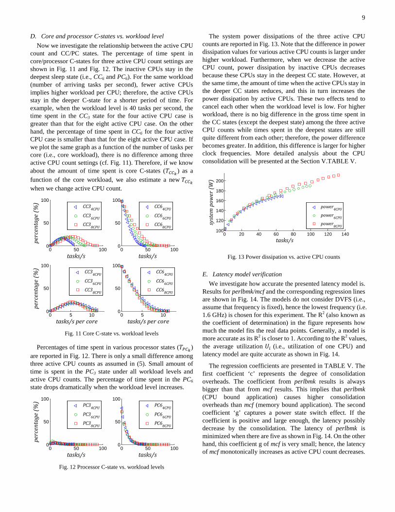
D. Core and processor C-states vs. workload level Now we investigate the relationship between the active CPU

count and CC/PC states. The percentage of time spent in core/processor C-states for three active CPU count settings are shown in Fig. 11 and Fig. 12. The inactive CPUs stay in the deepest sleep state (i.e., CC6 and PC6). For the same workload (number of arriving tasks per second), fewer active CPUs implies higher workload per CPU; therefore, the active CPUs stay in the deeper C-state for a shorter period of time. For example, when the workload level is 40 tasks per second, the time spent in the CC3 state for the four active CPU case is greater than that for the eight active CPU case. On the other hand, the percentage of time spent in CC6 for the four active CPU case is smaller than that for the eight active CPU case. If we plot the same graph as a function of the number of tasks per core (i.e., core workload), there is no difference among three active CPU count settings (cf. Fig. 11). Therefore, if we know about the amount of time spent is core C-states (𝑇𝐶𝐶𝑘) as a function of the core workload, we also estimate a new 𝑇𝐶𝐶𝑘 when we change active CPU count.

Fig. 11 Core C-state vs. workload levels

Percentages of time spent in various processor states (𝑇𝑃𝐶𝑘) are reported in Fig. 12. There is only a small difference among three active CPU counts as assumed in (5). Small amount of time is spent in the PC3 state under all workload levels and active CPU counts. The percentage of time spent in the PC6 state drops dramatically when the workload level increases.

Fig. 12 Processor C-state vs. workload levels

The system power dissipations of the three active CPU counts are reported in Fig. 13. Note that the difference in power dissipation values for various active CPU counts is larger under higher workload. Furthermore, when we decrease the active CPU count, power dissipation by inactive CPUs decreases because these CPUs stay in the deepest CC state. However, at the same time, the amount of time when the active CPUs stay in the deeper CC states reduces, and this in turn increases the power dissipation by active CPUs. These two effects tend to cancel each other when the workload level is low. For higher workload, there is no big difference in the gross time spent in the CC states (except the deepest state) among the three active CPU counts while times spent in the deepest states are still quite different from each other; therefore, the power difference becomes greater. In addition, this difference is larger for higher clock frequencies. More detailed analysis about the CPU consolidation will be presented at the Section V.TABLE V.

Fig. 13 Power dissipation vs. active CPU counts

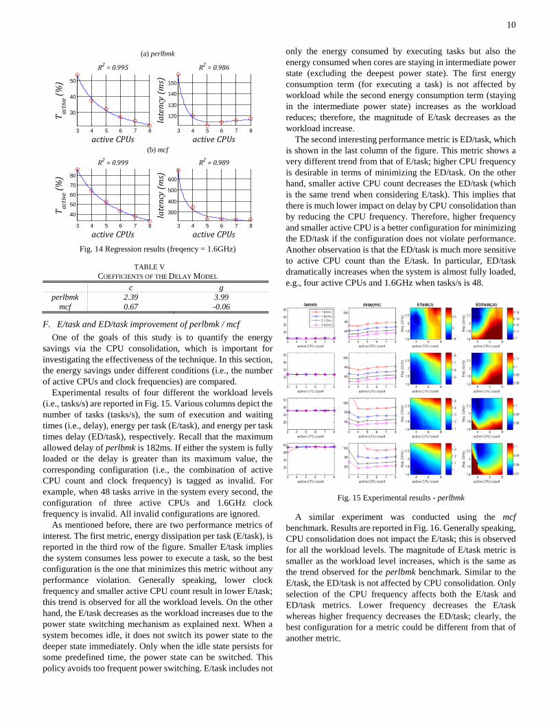
E. Latency model verification We investigate how accurate the presented latency model is.

Results for perlbmk/mcf and the corresponding regression lines are shown in Fig. 14. The models do not consider DVFS (i.e., assume that frequency is fixed), hence the lowest frequency (i.e. 1.6 GHz) is chosen for this experiment. The R2 (also known as the coefficient of determination) in the figure represents how much the model fits the real data points. Generally, a model is more accurate as its R2 is closer to 1. According to the R2 values, the average utilization 𝑈𝑖 (i.e., utilization of one CPU) and latency model are quite accurate as shown in Fig. 14.

The regression coefficients are presented in TABLE V. The first coefficient ‘c’ represents the degree of consolidation overheads. The coefficient from perlbmk results is always bigger than that from mcf results. This implies that perlbmk (CPU bound application) causes higher consolidation overheads than mcf (memory bound application). The second coefficient ‘g’ captures a power state switch effect. If the coefficient is positive and large enough, the latency possibly decrease by the consolidation. The latency of perlbmk is minimized when there are five as shown in Fig. 14. On the other hand, this coefficient g of mcf is very small; hence, the latency of mcf monotonically increases as active CPU count decreases.

0 50 1000

50

100

tasks/s

perc

enta

ge (%

)

CC34CPU

CC36CPU

CC38CPU

0 50 1000

50

100

tasks/s

CC64CPU

CC66CPU

CC68CPU

0 5 100

50

100

tasks/s per core

perc

enta

ge (%

)

CC34CPU

CC36CPU

CC38CPU

0 5 100

50

100

tasks/s per core

CC64CPU

CC66CPU

CC68CPU

0 50 1000

50

100

tasks/s

perc

enta

ge (%

)

PC34CPU

PC36CPU

PC38CPU

0 50 1000

50

100

tasks/s

PC64CPU

PC66CPU

PC68CPU

0 20 40 60 80 100 120 140100

120

140

160

180

200

tasks/s

syst

em p

ower

(W)

power4CPU

power6CPU

power8CPU

10

(a) perlbmk

(b) mcf

Fig. 14 Regression results (freqency = 1.6GHz)

TABLE V COEFFICIENTS OF THE DELAY MODEL

c g perlbmk 2.39 3.99

mcf 0.67 -0.06

F. E/task and ED/task improvement of perlbmk / mcf One of the goals of this study is to quantify the energy

savings via the CPU consolidation, which is important for investigating the effectiveness of the technique. In this section, the energy savings under different conditions (i.e., the number of active CPUs and clock frequencies) are compared.

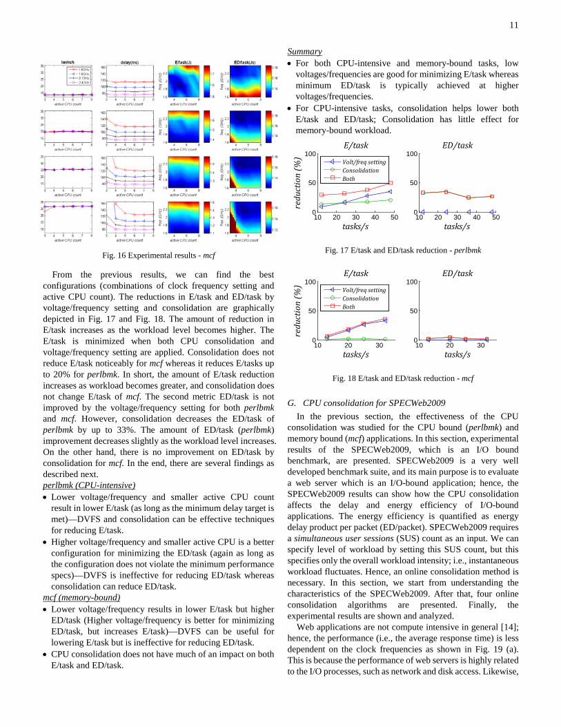
Experimental results of four different the workload levels (i.e., tasks/s) are reported in Fig. 15. Various columns depict the number of tasks (tasks/s), the sum of execution and waiting times (i.e., delay), energy per task (E/task), and energy per task times delay (ED/task), respectively. Recall that the maximum allowed delay of perlbmk is 182ms. If either the system is fully loaded or the delay is greater than its maximum value, the corresponding configuration (i.e., the combination of active CPU count and clock frequency) is tagged as invalid. For example, when 48 tasks arrive in the system every second, the configuration of three active CPUs and 1.6GHz clock frequency is invalid. All invalid configurations are ignored.

As mentioned before, there are two performance metrics of interest. The first metric, energy dissipation per task (E/task), is reported in the third row of the figure. Smaller E/task implies the system consumes less power to execute a task, so the best configuration is the one that minimizes this metric without any performance violation. Generally speaking, lower clock frequency and smaller active CPU count result in lower E/task; this trend is observed for all the workload levels. On the other hand, the E/task decreases as the workload increases due to the power state switching mechanism as explained next. When a system becomes idle, it does not switch its power state to the deeper state immediately. Only when the idle state persists for some predefined time, the power state can be switched. This policy avoids too frequent power switching. E/task includes not

only the energy consumed by executing tasks but also the energy consumed when cores are staying in intermediate power state (excluding the deepest power state). The first energy consumption term (for executing a task) is not affected by workload while the second energy consumption term (staying in the intermediate power state) increases as the workload reduces; therefore, the magnitude of E/task decreases as the workload increase.

The second interesting performance metric is ED/task, which is shown in the last column of the figure. This metric shows a very different trend from that of E/task; higher CPU frequency is desirable in terms of minimizing the ED/task. On the other hand, smaller active CPU count decreases the ED/task (which is the same trend when considering E/task). This implies that there is much lower impact on delay by CPU consolidation than by reducing the CPU frequency. Therefore, higher frequency and smaller active CPU is a better configuration for minimizing the ED/task if the configuration does not violate performance. Another observation is that the ED/task is much more sensitive to active CPU count than the E/task. In particular, ED/task dramatically increases when the system is almost fully loaded, e.g., four active CPUs and 1.6GHz when tasks/s is 48.

Fig. 15 Experimental results - perlbmk

A similar experiment was conducted using the mcf benchmark. Results are reported in Fig. 16. Generally speaking, CPU consolidation does not impact the E/task; this is observed for all the workload levels. The magnitude of E/task metric is smaller as the workload level increases, which is the same as the trend observed for the perlbmk benchmark. Similar to the E/task, the ED/task is not affected by CPU consolidation. Only selection of the CPU frequency affects both the E/task and ED/task metrics. Lower frequency decreases the E/task whereas higher frequency decreases the ED/task; clearly, the best configuration for a metric could be different from that of another metric.

3 4 5 6 7 8

30

40

50

R2 = 0.995T ac

tive (%

)

active CPUs3 4 5 6 7 8

120

130

140

150

active CPUs

R2 = 0.986

late

ncy

(ms)

3 4 5 6 7 8

40

50

60

70

80

R2 = 0.999

T activ

e (%)

active CPUs3 4 5 6 7 8

300

400

500

600

active CPUs

R2 = 0.989la

tenc

y (m

s)

11

Fig. 16 Experimental results - mcf

From the previous results, we can find the best configurations (combinations of clock frequency setting and active CPU count). The reductions in E/task and ED/task by voltage/frequency setting and consolidation are graphically depicted in Fig. 17 and Fig. 18. The amount of reduction in E/task increases as the workload level becomes higher. The E/task is minimized when both CPU consolidation and voltage/frequency setting are applied. Consolidation does not reduce E/task noticeably for mcf whereas it reduces E/tasks up to 20% for perlbmk. In short, the amount of E/task reduction increases as workload becomes greater, and consolidation does not change E/task of mcf. The second metric ED/task is not improved by the voltage/frequency setting for both perlbmk and mcf. However, consolidation decreases the ED/task of perlbmk by up to 33%. The amount of ED/task (perlbmk) improvement decreases slightly as the workload level increases. On the other hand, there is no improvement on ED/task by consolidation for mcf. In the end, there are several findings as described next. perlbmk (CPU-intensive) • Lower voltage/frequency and smaller active CPU count

result in lower E/task (as long as the minimum delay target is met)—DVFS and consolidation can be effective techniques for reducing E/task.

• Higher voltage/frequency and smaller active CPU is a better configuration for minimizing the ED/task (again as long as the configuration does not violate the minimum performance specs)—DVFS is ineffective for reducing ED/task whereas consolidation can reduce ED/task.

mcf (memory-bound) • Lower voltage/frequency results in lower E/task but higher

ED/task (Higher voltage/frequency is better for minimizing ED/task, but increases E/task)—DVFS can be useful for lowering E/task but is ineffective for reducing ED/task.

• CPU consolidation does not have much of an impact on both E/task and ED/task.

Summary • For both CPU-intensive and memory-bound tasks, low

voltages/frequencies are good for minimizing E/task whereas minimum ED/task is typically achieved at higher voltages/frequencies.

• For CPU-intensive tasks, consolidation helps lower both E/task and ED/task; Consolidation has little effect for memory-bound workload.

Fig. 17 E/task and ED/task reduction - perlbmk

Fig. 18 E/task and ED/task reduction - mcf

G. CPU consolidation for SPECWeb2009 In the previous section, the effectiveness of the CPU

consolidation was studied for the CPU bound (perlbmk) and memory bound (mcf) applications. In this section, experimental results of the SPECWeb2009, which is an I/O bound benchmark, are presented. SPECWeb2009 is a very well developed benchmark suite, and its main purpose is to evaluate a web server which is an I/O-bound application; hence, the SPECWeb2009 results can show how the CPU consolidation affects the delay and energy efficiency of I/O-bound applications. The energy efficiency is quantified as energy delay product per packet (ED/packet). SPECWeb2009 requires a simultaneous user sessions (SUS) count as an input. We can specify level of workload by setting this SUS count, but this specifies only the overall workload intensity; i.e., instantaneous workload fluctuates. Hence, an online consolidation method is necessary. In this section, we start from understanding the characteristics of the SPECWeb2009. After that, four online consolidation algorithms are presented. Finally, the experimental results are shown and analyzed.

Web applications are not compute intensive in general [14]; hence, the performance (i.e., the average response time) is less dependent on the clock frequencies as shown in Fig. 19 (a). This is because the performance of web servers is highly related to the I/O processes, such as network and disk access. Likewise,

10 20 30 40 500

50

100E/task

tasks/s

redu

ctio

n (%

)

Volt/freq settingConsolidationBoth

10 20 30 40 500

50

100ED/task

tasks/s

10 20 300

50

100E/task

tasks/s

redu

ctio

n (%

)

Volt/freq settingConsolidationBoth

10 20 300

50

100ED/task

tasks/s

12

the performance is almost independent of the active CPU count if a sufficient number of CPUs is active. The relationship between the power dissipation and frequencies/active CPU count is shown in Fig. 19 (b). The amount of power dissipation declines as the frequency becomes lower and/or the active CPU count is reduced. This result implies that both DVFS and the CPU consolidation improve the energy efficiency without significant performance degradation. In addition, we expect the further improvement when both techniques are applied at the same time.

Fig. 19 Response time and power dissipation

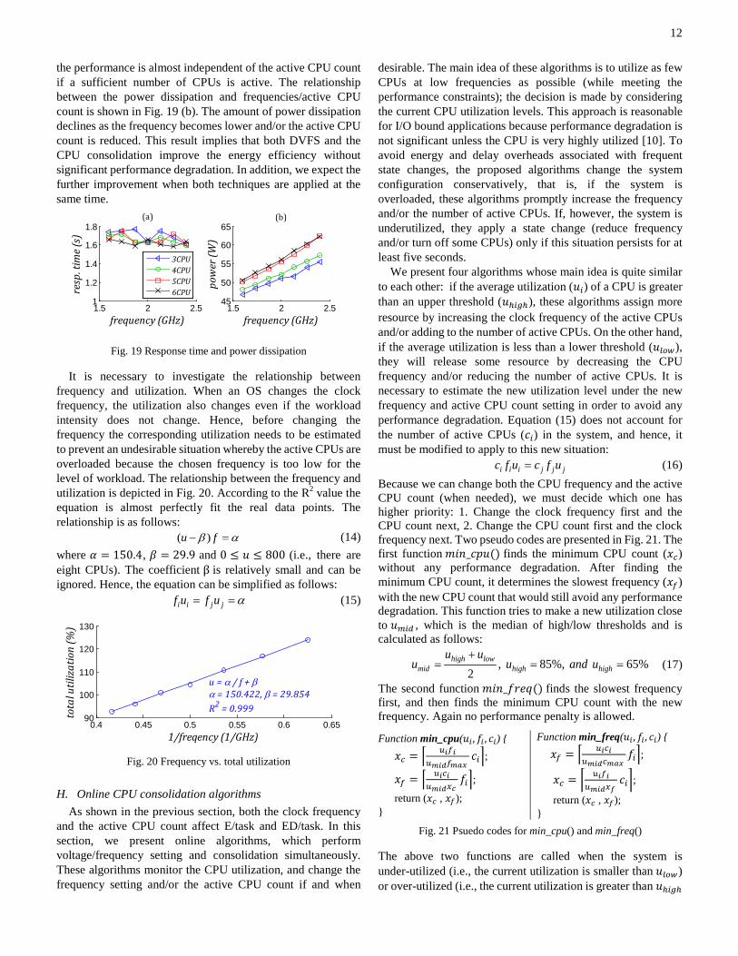
It is necessary to investigate the relationship between frequency and utilization. When an OS changes the clock frequency, the utilization also changes even if the workload intensity does not change. Hence, before changing the frequency the corresponding utilization needs to be estimated to prevent an undesirable situation whereby the active CPUs are overloaded because the chosen frequency is too low for the level of workload. The relationship between the frequency and utilization is depicted in Fig. 20. According to the R2 value the equation is almost perfectly fit the real data points. The relationship is as follows:

( )u fβ α− = (14) where 𝛼 = 150.4, 𝛽 = 29.9 and 0 ≤ 𝑢 ≤ 800 (i.e., there are eight CPUs). The coefficient β is relatively small and can be ignored. Hence, the equation can be simplified as follows:

i i j jf u f u α= = (15)

Fig. 20 Frequency vs. total utilization

H. Online CPU consolidation algorithms As shown in the previous section, both the clock frequency

and the active CPU count affect E/task and ED/task. In this section, we present online algorithms, which perform voltage/frequency setting and consolidation simultaneously. These algorithms monitor the CPU utilization, and change the frequency setting and/or the active CPU count if and when

desirable. The main idea of these algorithms is to utilize as few CPUs at low frequencies as possible (while meeting the performance constraints); the decision is made by considering the current CPU utilization levels. This approach is reasonable for I/O bound applications because performance degradation is not significant unless the CPU is very highly utilized [10]. To avoid energy and delay overheads associated with frequent state changes, the proposed algorithms change the system configuration conservatively, that is, if the system is overloaded, these algorithms promptly increase the frequency and/or the number of active CPUs. If, however, the system is underutilized, they apply a state change (reduce frequency and/or turn off some CPUs) only if this situation persists for at least five seconds.

We present four algorithms whose main idea is quite similar to each other: if the average utilization (𝑢𝑖) of a CPU is greater than an upper threshold (𝑢ℎ𝑖𝑔ℎ), these algorithms assign more resource by increasing the clock frequency of the active CPUs and/or adding to the number of active CPUs. On the other hand, if the average utilization is less than a lower threshold (𝑢𝑙𝑜𝑤), they will release some resource by decreasing the CPU frequency and/or reducing the number of active CPUs. It is necessary to estimate the new utilization level under the new frequency and active CPU count setting in order to avoid any performance degradation. Equation (15) does not account for the number of active CPUs (𝑐𝑖) in the system, and hence, it must be modified to apply to this new situation:

i i i j j jc f u c f u= (16) Because we can change both the CPU frequency and the active CPU count (when needed), we must decide which one has higher priority: 1. Change the clock frequency first and the CPU count next, 2. Change the CPU count first and the clock frequency next. Two pseudo codes are presented in Fig. 21. The first function 𝑚𝑖𝑛_𝑐𝑝𝑢() finds the minimum CPU count (𝑥𝑐) without any performance degradation. After finding the minimum CPU count, it determines the slowest frequency (𝑥𝑓) with the new CPU count that would still avoid any performance degradation. This function tries to make a new utilization close to 𝑢𝑚𝑖𝑑 , which is the median of high/low thresholds and is calculated as follows:

, 85%, 65%2

high lowmid high high

u uu u and u

+= = = (17)

The second function 𝑚𝑖𝑛_𝑓𝑟𝑒𝑞() finds the slowest frequency first, and then finds the minimum CPU count with the new frequency. Again no performance penalty is allowed.

Function min_cpu(𝑢𝑖 , 𝑓𝑖 , 𝑐𝑖) { 𝑥𝑐 = � 𝑢𝑖𝑓𝑖

𝑢𝑚𝑖𝑑𝑓𝑚𝑎𝑥 𝑐𝑖�;

𝑥𝑓 = � 𝑢𝑖𝑐𝑖𝑢𝑚𝑖𝑑𝑥𝑐

𝑓𝑖�; return (𝑥𝑐 , 𝑥𝑓); }

Function min_freq(𝑢𝑖 , 𝑓𝑖 , 𝑐𝑖) { 𝑥𝑓 = � 𝑢𝑖𝑐𝑖

𝑢𝑚𝑖𝑑𝑐𝑚𝑎𝑥 𝑓𝑖�;

𝑥𝑐 = � 𝑢𝑖𝑓𝑖𝑢𝑚𝑖𝑑𝑥𝑓

𝑐𝑖�; return (𝑥𝑐 , 𝑥𝑓); }

Fig. 21 Psuedo codes for min_cpu() and min_freq()

The above two functions are called when the system is under-utilized (i.e., the current utilization is smaller than 𝑢𝑙𝑜𝑤) or over-utilized (i.e., the current utilization is greater than 𝑢ℎ𝑖𝑔ℎ

1.5 2 2.51

1.2

1.4

1.6

1.8(a)

frequency (GHz)

resp

. tim

e (s)

3CPU4CPU5CPU6CPU

1.5 2 2.545

50

55

60

65(b)

frequency (GHz)

pow

er (W

)

0.4 0.45 0.5 0.55 0.6 0.6590

100

110

120

130

1/freqency (1/GHz)

tota

l util

izat

ion

(%)

u = α / f + βα = 150.422, β = 29.854R2 = 0.999

13

). For each case, we can choose which function is called, i.e., 𝑚𝑖𝑛_𝑐𝑝𝑢() or 𝑚𝑖𝑛_𝑓𝑟𝑒𝑞(). Therefore, there are a total of four online algorithms, which are shown in Fig. 22. The first algorithm (type1) calls 𝑚𝑖𝑛_𝑐𝑝𝑢() function for both the under and over-utilized CPU cases. The type2 algorithm calls 𝑚𝑖𝑛_𝑐𝑝𝑢() when a CPU is over-utilized and 𝑚𝑖𝑛_𝑓𝑟𝑒𝑞() if it is under-utilized. The type3 algorithm calls 𝑚𝑖𝑛_𝑓𝑟𝑒𝑞() when a CPU is over-utilized and 𝑚𝑖𝑛_𝑐𝑝𝑢() if it is under-utilized. The last algorithm (type4) calls 𝑚𝑖𝑛_𝑓𝑟𝑒𝑞() for both over and under-utilized CPU cases.

Fig. 22 Four online consolidation algorithms

We do experiments for three different SUS counts and compare the energy-delay product per packet (ED/packet) and the quality of service (QoS) for the aforesaid four consolidation algorithms and two more baseline algorithms. The QoS refers to the percentage of packets for which delay is less than a pre-defined limit. This QoS is reported by SPECWeb2009 benchmark suite. In addition to the four proposed algorithms, we provide results for two other algorithms: base and ondemand. The base algorithm means there is no dynamic adjustment of the active CPU count and frequency, i.e., frequency is the highest one and all CPUs are active. The ondemand algorithm is the default voltage/frequency setting method used in LinuxTM, which does not change the active CPU count but changes the CPU frequency (all CPUs will have the same frequency at any time).

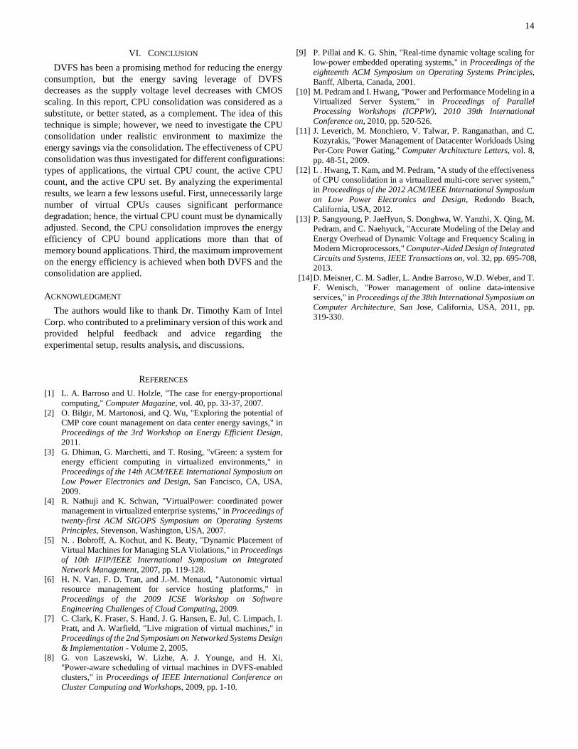
Experimental results are reported in Fig. 23. Regardless of the SUS counts, the proposed algorithms always result in smaller ED/packet compared to the base and ondemand algorithms. Among the four proposed algorithms, type1 algorithm is the best one in terms of ED/packet. As the SUS count increases, QoS of all algorithms decreases, but QoS remains greater than 95%; hence, there are no performance degradation concerns. Note that the magnitude of ED/packet metric also decreases as the SUS count increases, which implies that the system consumes less energy for executing a packet. This is because of the energy non-proportionality of the existing server systems (including the one used in this study). From these results, we can state that the type1 consolidation algorithm is the best. This implies that, at least for the system under experiment, adjusting the CPU frequency has higher impact on the ED/packet metric than changing the CPU count.

(a) SUS=1000

(b) SUS=1400

(c) SUS=1900

Fig. 23 ED/pack and QoS comparisons

We compare ED/packet of the ondemand and type1 algorithm, which is shown in TABLE VI. For three SUS settings, ED/packet of type1 algorithm is always smaller than that of ondemand. In addition, the difference between them increases for the larger number of user sessions.

TABLE VI COEFFICIENTS OF THE DELAY MODEL

SUS ED/packet (Js) ∆ED/packet(%) ondemand type1

1000 0.91 0.82 9.44 1400 0.76 0.67 11.83 1900 0.51 0.44 13.648

14

VI. CONCLUSION DVFS has been a promising method for reducing the energy

consumption, but the energy saving leverage of DVFS decreases as the supply voltage level decreases with CMOS scaling. In this report, CPU consolidation was considered as a substitute, or better stated, as a complement. The idea of this technique is simple; however, we need to investigate the CPU consolidation under realistic environment to maximize the energy savings via the consolidation. The effectiveness of CPU consolidation was thus investigated for different configurations: types of applications, the virtual CPU count, the active CPU count, and the active CPU set. By analyzing the experimental results, we learn a few lessons useful. First, unnecessarily large number of virtual CPUs causes significant performance degradation; hence, the virtual CPU count must be dynamically adjusted. Second, the CPU consolidation improves the energy efficiency of CPU bound applications more than that of memory bound applications. Third, the maximum improvement on the energy efficiency is achieved when both DVFS and the consolidation are applied.

ACKNOWLEDGMENT The authors would like to thank Dr. Timothy Kam of Intel

Corp. who contributed to a preliminary version of this work and provided helpful feedback and advice regarding the experimental setup, results analysis, and discussions.

REFERENCES [1] L. A. Barroso and U. Holzle, "The case for energy-proportional

computing," Computer Magazine, vol. 40, pp. 33-37, 2007. [2] O. Bilgir, M. Martonosi, and Q. Wu, "Exploring the potential of

CMP core count management on data center energy savings," in Proceedings of the 3rd Workshop on Energy Efficient Design, 2011.

[3] G. Dhiman, G. Marchetti, and T. Rosing, "vGreen: a system for energy efficient computing in virtualized environments," in Proceedings of the 14th ACM/IEEE International Symposium on Low Power Electronics and Design, San Fancisco, CA, USA, 2009.

[4] R. Nathuji and K. Schwan, "VirtualPower: coordinated power management in virtualized enterprise systems," in Proceedings of twenty-first ACM SIGOPS Symposium on Operating Systems Principles, Stevenson, Washington, USA, 2007.

[5] N. . Bobroff, A. Kochut, and K. Beaty, "Dynamic Placement of Virtual Machines for Managing SLA Violations," in Proceedings of 10th IFIP/IEEE International Symposium on Integrated Network Management, 2007, pp. 119-128.

[6] H. N. Van, F. D. Tran, and J.-M. Menaud, "Autonomic virtual resource management for service hosting platforms," in Proceedings of the 2009 ICSE Workshop on Software Engineering Challenges of Cloud Computing, 2009.

[7] C. Clark, K. Fraser, S. Hand, J. G. Hansen, E. Jul, C. Limpach, I. Pratt, and A. Warfield, "Live migration of virtual machines," in Proceedings of the 2nd Symposium on Networked Systems Design & Implementation - Volume 2, 2005.

[8] G. von Laszewski, W. Lizhe, A. J. Younge, and H. Xi, "Power-aware scheduling of virtual machines in DVFS-enabled clusters," in Proceedings of IEEE International Conference on Cluster Computing and Workshops, 2009, pp. 1-10.

[9] P. Pillai and K. G. Shin, "Real-time dynamic voltage scaling for low-power embedded operating systems," in Proceedings of the eighteenth ACM Symposium on Operating Systems Principles, Banff, Alberta, Canada, 2001.

[10] M. Pedram and I. Hwang, "Power and Performance Modeling in a Virtualized Server System," in Proceedings of Parallel Processing Workshops (ICPPW), 2010 39th International Conference on, 2010, pp. 520-526.

[11] J. Leverich, M. Monchiero, V. Talwar, P. Ranganathan, and C. Kozyrakis, "Power Management of Datacenter Workloads Using Per-Core Power Gating," Computer Architecture Letters, vol. 8, pp. 48-51, 2009.

[12] I. . Hwang, T. Kam, and M. Pedram, "A study of the effectiveness of CPU consolidation in a virtualized multi-core server system," in Proceedings of the 2012 ACM/IEEE International Symposium on Low Power Electronics and Design, Redondo Beach, California, USA, 2012.

[13] P. Sangyoung, P. JaeHyun, S. Donghwa, W. Yanzhi, X. Qing, M. Pedram, and C. Naehyuck, "Accurate Modeling of the Delay and Energy Overhead of Dynamic Voltage and Frequency Scaling in Modern Microprocessors," Computer-Aided Design of Integrated Circuits and Systems, IEEE Transactions on, vol. 32, pp. 695-708, 2013.

[14] D. Meisner, C. M. Sadler, L. Andre Barroso, W.D. Weber, and T. F. Wenisch, "Power management of online data-intensive services," in Proceedings of the 38th International Symposium on Computer Architecture, San Jose, California, USA, 2011, pp. 319-330.

15

APPENDIX We start by estimating the power dissipation when the

C-state limit is C1. In this case, there are two CC states and two PC states: CC0, CC1, PC0, and PC1. If more than one sleep state is available, the power dissipation is supposed to decrease super-linearly as the utilization decreases. This is because the amount of time spent in deeper sleep states is greater when the utilization is lower. The measured power dissipation, however, is linearly proportional to CPU utilization, as reported in Fig. 9. This linearity can be explained once we realize that the C-state of core/processor is promptly switched to the deepest sleep state, i.e., CC1 and PC1, that is, in our target system the amount of time spent in CC0 and PC0 is very small. The power dissipation is a linear function of utilization, so we can easily estimate the power dissipation using the utilization level (𝑈𝑡𝑖𝑙):

. 21.88 141.12totalest activeP T= + (18)

If we set the deepest C-state to C2, there is no longer a linear relationship between the utilization and the power dissipation as reported in Fig. 9To explain this behavior, recall that total (platform) power dissipation is the sum of the processor power dissipation and the power consumed by other components:

icoretotal uncore otheriP P P P= + +∑ (19)

General purpose CPU schedulers evenly distribute tasks to active CPUs. Because we have eight CPUs, the total power dissipation is:

8total core uncore otherP P P P= + + (20) Calculating the difference between power dissipations for two cases, i.e., case 1 where the C-state limit is C1 (up to CC1/PC1 are available) and case 2 where the C-state limit is C2 (up to CC3/PC3 are available), we write:

( ) ( )1 2 1 2

8

8

total core uncore

core core uncore uncoreC C C C

P P P

P P P P

∆ = ∆ + ∆

= − + − (21)

Notice that the power difference equation does not include the difference of 𝑃𝑜𝑡ℎ𝑒𝑟 terms because the C-state limit does not change power consumptions of other components.

The core power dissipation can be formulated by using the utilization level and the time spent in each core C-state (i.e., CC0, CC1, and CC3). The core power dissipations when the C-state limit is C1 and C2 are:

1 0 0 1 1

2 0 0 1 1 3 3

core core core coreC active active CC CC CC CC

core core core core coreC active active CC CC CC CC CC CC

P P T P x P x

P P T P y P y P T

= + +

= + + + (22)

where 𝑥𝐶𝐶0 + 𝑥𝐶𝐶1 = 1 − 𝑇𝑎𝑐𝑡𝑖𝑣𝑒 and 𝑦𝐶𝐶0 + 𝑦𝐶𝐶1 = 1 −𝑇𝑎𝑐𝑡𝑖𝑣𝑒 − 𝑇𝐶𝐶3 . In above equations 𝑥𝐶𝐶𝑛 and 𝑦𝐶𝐶𝑛 are the percentages of time spent in the 𝐶𝐶𝑛 state when the C-state limit is C1 and C2, respectively (these parameters are not reported by the system hardware as shown in TABLE III). The power difference is:

( ) ( )

1 2

0 0 0 1 1 1 3 3

core core coreC C

core core coreCC CC CC CC CC CC CC CC

P P P

P x y P x y P T

∆ = −

= − + − −(23)

For simplicity, we state that 𝑥𝐶𝐶0 = 𝑦𝐶𝐶0 . This implies a core stays in the CC0 power state for the same amount of time under

the same utilization levels regardless of the C-state limit. Thus, we have:

( )1 1 1 3 3core core core

CC CC CC CC CCP P x y P T∆ = − − (24)

If we make the assumption that 𝑥𝐶𝐶0 = 𝑦𝐶𝐶0 = 0 (this is because power dissipation is ONLY linearly dependent on the utilization level when the C-state limit is C1; note that the non-linear power dissipation vs. utilization graph for the case that the C-state limit is C2 cannot be used to confirm or reject this assumption), the power difference can be re-written as below:

( ) ( )( )

( )1 3

3 3 1 3 3

1 1

core coreCC active active CC

core core coreCC CC CC CC CC

P P T T T

P T P P T

∆ = − − − −

− = − (25)

Similarly, the uncore power dissipations when the C-state limit is C1 and C2 are:

1 0 0 0 1 1

2 30 0 0 1 1 3

uncore uncore uncore uncoreC PC active PC PC PC PC

uncore uncore uncore uncore uncoreC PC active PC PC PC PC PC PC

P P T P k P k

P P T P h P h P T

= + +

= + + +(26)

where 𝑘𝑃𝐶0 + 𝑘𝑃𝐶1 = 1 − 𝑈𝑡𝑖𝑙 and ℎ𝑃𝐶0 + ℎ𝑃𝐶1 = 1 − 𝑈𝑡𝑖𝑙 −𝑃𝐶3. With a similar assumption that 𝑘𝑃𝐶0 = ℎ𝑃𝐶0 = 0, we have:

( ) ( )( )

( )1 3

3 3 1 3 3

1 1

uncore uncorePC active active PC

uncore uncore uncorePC PC PC PC PC

P P T T T

P T P P T

∆ = − − − −

− = − (27)

Finally, the difference in the total power dissipation is:

( ) ( )1 3 3 1 3 3

8

8

total core uncore

core core uncore uncoreCC CC CC PC PC PC

P P P

P P T P P T

∆ = ∆ + ∆

= − + − (28)

In the above equation, �𝑃𝐶𝐶1𝑐𝑜𝑟𝑒 − 𝑃𝐶𝐶3_

𝑐𝑜𝑟𝑒� and �𝑃𝑃𝐶1𝑢𝑛𝑐𝑜𝑟𝑒 −

𝑃𝑃𝐶3_𝑢𝑛𝑐𝑜𝑟𝑒� are unknown parameters to be determined. The total

power dissipation, the percentage of time in the core C-states (𝐶𝐶3 and 𝐶𝐶6), and the percentage of time in the processor C-states (𝑃𝐶3 and 𝑃𝐶6 ) are reported in TABLE VII. The difference in the total power dissipation when all cores are idle is:

( ) ( )1 3 1 308 1.0 0.79

140.7 -110.3 30.4

total core core uncore uncoreCC CC PC PCutil

P P P P P

W=

∆ = − × + − ×

= =(29)

Therefore, we can calculate �𝑃𝑃𝐶1𝑢𝑛𝑐𝑜𝑟𝑒 − 𝑃𝑃𝐶3_

𝑢𝑛𝑐𝑜𝑟𝑒� as a function of �𝑃𝐶𝐶1

𝑐𝑜𝑟𝑒 − 𝑃𝐶𝐶3_𝑐𝑜𝑟𝑒�:

( )1 3 1 338.48 8 1.27uncore uncore core core

PC PC CC CCP P P P− = − − × (30) TABLE VII

POWER DISSIPATION AND C-STATES WHEN EVERY CORE IS IDLE

C-state limit

Utilization (%)

Core C-state

Processor C-state Power

(W) CC3 CC6 PC3 PC6 C1 0 n/a n/a n/a n/a 140.7 C2 0 99.0 n/a 79.1 n/a 110.3 C3 0 0.0 99.9 0.0 79.9 98.1

Next, we obtain value of �𝑃𝐶𝐶1𝑐𝑜𝑟𝑒 − 𝑃𝐶𝐶3

𝑐𝑜𝑟𝑒� by changing the active CPU count. Note that in experimental results reported above, we always had eight active CPUs whereas in the results to be reported next, the active CPU count is changed. If 𝑚 CPUs are active and fully utilized, (8 −𝑚) CPUs are inactive

16

and in the deepest power state (𝐶𝐶𝑘). Therefore, the total power dissipation in this case is:

( )

( ) 8

coretotal uncore otherii

core core uncore otheractive CCk

P m P P P

mP m P P P

= + +

= + − + +

∑ (31)

If another CPU becomes active, i.e. there will be (𝑚 + 1) active CPUs, and the total power dissipation will be:

( ) ( ) ( ) '1 1 7total core core uncore otheractive CCk

P m m P m P P P+ = + + − + + (32)

The power dissipation of other parts (𝑃𝑜𝑡ℎ𝑒𝑟 ) can be affected by the active CPU count because the number of tasks served by the system increases as the active CPU count increases. Note that all active CPUs are fully utilized, i.e., 100% utilization, hence, more active CPU count means higher throughput (i.e., the number of tasks served per second). However, we assume power dissipation by other parts of 𝑚 active CPUs is not very different from that of (𝑚 + 1) active CPUs: 𝑃𝑜𝑡ℎ𝑒𝑟 ≅ 𝑃𝑜𝑡ℎ𝑒𝑟′. Consequently, we have:

( ) ( ) ( )1total total core coreactive CCk

P m P m P P+ − ≅ − (33)

The left term of the above equation can be obtained by experiments, so we can find (𝑃𝐶𝐶1 − 𝑃𝐶𝐶3) as follows:

( ) ( )1 3 3 1

( ,3) ( ,1)

core core core core core coreCC CC active CC active CCP P P P P P

g m g m

− = − − −

= − (34)

where ( ) ( )

( , ) 1total total

deepest CC state CCkg m k P m P m

= = + − .

The right term in the above equation is a function of active CPU count (𝑛), but it does not make sense because �𝑃𝐶𝐶1

𝑐𝑜𝑟𝑒 − 𝑃𝐶𝐶3_𝑐𝑜𝑟𝑒�

is supposed to be constant and not a function of 𝑛 . The experimental results imply that �𝑃𝐶𝐶1

𝑐𝑜𝑟𝑒 − 𝑃𝐶𝐶3_𝑐𝑜𝑟𝑒� is not a

function of 𝑛 as shown in Fig. 24. This figure shows the power dissipation when all active cores are fully utilized with three different C-state limits. The slope of a plot in this figure is 𝑔(𝑚, 𝑘) , and is independent of the active CPU count 𝑛 (i.e., 𝑔(𝑚, 𝑘) = 𝑔(𝑘)) because the slope is constant (linear plot). Therefore, we can find �𝑃𝐶𝐶1

𝑐𝑜𝑟𝑒 − 𝑃𝐶𝐶3_𝑐𝑜𝑟𝑒� and �𝑃𝐶𝐶1

𝑐𝑜𝑟𝑒 −𝑃𝐶𝐶6_𝑐𝑜𝑟𝑒� as follows:

1 3

1 6

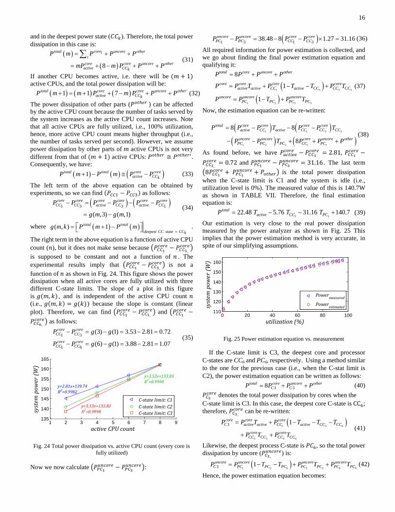
(3) (1) 3.53 2.81 0.72

(6) (1) 3.88 2.81 1.07

core coreCC CC

core coreCC CC

P P g g

P P g g

− = − = − =

− = − = − = (35)

Fig. 24 Total power dissipation vs. active CPU count (every core is fully utilized)

Now we now calculate �𝑃𝑃𝐶1𝑢𝑛𝑐𝑜𝑟𝑒 − 𝑃𝑃𝐶3

𝑢𝑛𝑐𝑜𝑟𝑒�:

( )1 3 1 338.48 8 1.27 31.16uncore uncore core core

PC PC CC CCP P P P− = − − × = (36)

All required information for power estimation is collected, and we go about finding the final power estimation equation and qualifying it:

( )( )

1 3 3 3

1 3 3 3

8

1

1

total core uncore other

core core core coreactive active CC active CC CC CC

uncore uncore uncorePC PC PC PC

P P P P

P P T P T T P T

P P T P T

= + +

= + − − +

= − +

(37)

Now, the estimation equation can be re-written:

( ) ( )

( ) ( )1 1 3 3

1 3 3 1 1

8 8

8

total core core core coreactive CC active CC CC CC

uncore uncore core uncore otherPC PC PC CC PC

P P P T P P T

P P T P P P

= − − −

− − + + +(38)

As found before, we have 𝑃𝑎𝑐𝑡𝑖𝑣𝑒𝑐𝑜𝑟𝑒 − 𝑃𝐶𝐶1𝑐𝑜𝑟𝑒 = 2.81, 𝑃𝐶𝐶1

𝑐𝑜𝑟𝑒 −𝑃𝐶𝐶3_𝑐𝑜𝑟𝑒 = 0.72 and 𝑃𝑃𝐶1

𝑢𝑛𝑐𝑜𝑟𝑒 − 𝑃𝑃𝐶3𝑢𝑛𝑐𝑜𝑟𝑒 = 31.16 . The last term

�8𝑃𝐶𝐶1𝑐𝑜𝑟𝑒 + 𝑃𝑃𝐶1

𝑢𝑛𝑐𝑜𝑟𝑒 + 𝑃𝑜𝑡ℎ𝑒𝑟� is the total power dissipation when the C-state limit is C1 and the system is idle (i.e., utilization level is 0%). The measured value of this is 140.7W as shown in TABLE VII. Therefore, the final estimation equation is:

3 3

22.48 5.76 31.16 140.7totalactive CC PCP T T T= − − + (39)

Our estimation is very close to the real power dissipation measured by the power analyzer as shown in Fig. 25 This implies that the power estimation method is very accurate, in spite of our simplifying assumptions.

Fig. 25 Power estimation equation vs. measurement

If the C-state limit is C3, the deepest core and processor C-states are CC6 and PC6, respectively. Using a method similar to the one for the previous case (i.e., when the C-stat limit is C2), the power estimation equation can be written as follows:

(40) 𝑃𝐶3𝑐𝑜𝑟𝑒 denotes the total power dissipation by cores when the

C-state limit is C3. In this case, the deepest core C-state is CC6; therefore, 𝑃𝐶3_

𝑐𝑜𝑟𝑒 can be re-written:

( )1 3 6

3 3 6 6

3 1

core core coreC active active CC active CC CC

core coreCC CC CC CC

P P T P T T T

P T P T

= + − − −

+ + (41)

Likewise, the deepest process C-state is 𝑃𝐶6, so the total power dissipation by uncore (𝑃𝐶3_

𝑢𝑛𝑐𝑜𝑟𝑒) is:

( )1 3 6 3 3 6 63 1uncore uncore uncore uncoreC PC PC PC PC PC PC PCP P T T P T P T= − − + + (42)

Hence, the power estimation equation becomes:

1 2 3 4 5 6 7 8 9135

140

145

150

155

160

165

active CPU count

syst

em p

ower

(W)

y=2.81x+139.74R2=0.9982

y=3.53x+133.83R2=0.9998

y=3.53x+133.83R2=0.9998

C-state limit: C1C-state limit: C2C-state limit: C3

0 20 40 60 80 100110

120

130

140

150

160

utilization (%)

syst

em p

ower

(W)

Powermeasured

Powerestimated

3 38total core uncore otherC CP P P P= + +

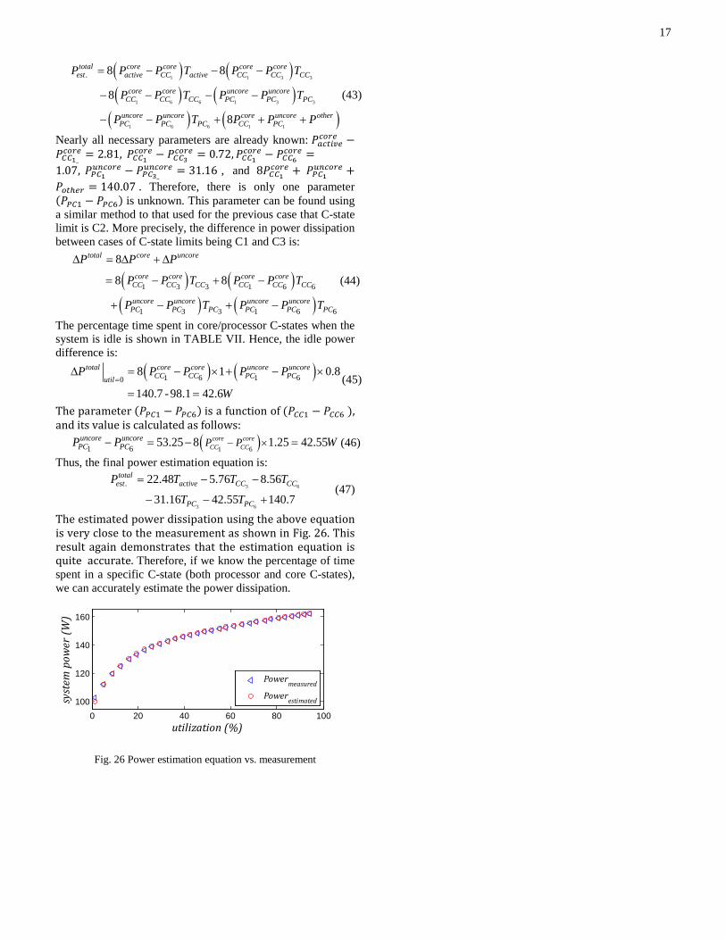
17

( ) ( )( ) ( )

( ) ( )

1 1 3 3

1 6 6 1 3 3

1 6 6 1 1

. 8 8

8

8

total core core core coreest active CC active CC CC CC

core core uncore uncoreCC CC CC PC PC PC

uncore uncore core uncore otherPC PC PC CC PC

P P P T P P T

P P T P P T

P P T P P P

= − − −

− − − −

− − + + +

(43)

Nearly all necessary parameters are already known: 𝑃𝑎𝑐𝑡𝑖𝑣𝑒𝑐𝑜𝑟𝑒 −𝑃𝐶𝐶1_𝑐𝑜𝑟𝑒 = 2.81, 𝑃𝐶𝐶1

𝑐𝑜𝑟𝑒 − 𝑃𝐶𝐶3𝑐𝑜𝑟𝑒 = 0.72,𝑃𝐶𝐶1

𝑐𝑜𝑟𝑒 − 𝑃𝐶𝐶6𝑐𝑜𝑟𝑒 =

1.07, 𝑃𝑃𝐶1𝑢𝑛𝑐𝑜𝑟𝑒 − 𝑃𝑃𝐶3_

𝑢𝑛𝑐𝑜𝑟𝑒 = 31.16 , and 8𝑃𝐶𝐶1𝑐𝑜𝑟𝑒 + 𝑃𝑃𝐶1

𝑢𝑛𝑐𝑜𝑟𝑒 +𝑃𝑜𝑡ℎ𝑒𝑟 = 140.07 . Therefore, there is only one parameter (𝑃𝑃𝐶1 − 𝑃𝑃𝐶6) is unknown. This parameter can be found using a similar method to that used for the previous case that C-state limit is C2. More precisely, the difference in power dissipation between cases of C-state limits being C1 and C3 is:

( ) ( )( ) ( )

1 3 3 1 6 6

1 3 3 1 6 6

8

8 8

total core uncore

core core core coreCC CC CC CC CC CC

uncore uncore uncore uncorePC PC PC PC PC PC

P P P

P P T P P T

P P T P P T

∆ = ∆ + ∆

= − + −

+ − + −

(44)

The percentage time spent in core/processor C-states when the system is idle is shown in TABLE VII. Hence, the idle power difference is:

( ) ( )1 6 1 608 1 0.8

140.7 - 98.1 42.6

total core core uncore uncoreCC CC PC PCutil

P P P P P

W=

∆ = − × + − ×

= =(45)

The parameter (𝑃𝑃𝐶1 − 𝑃𝑃𝐶6) is a function of (𝑃𝐶𝐶1 − 𝑃𝐶𝐶6 ), and its value is calculated as follows:

( )1 61 653.25 8 1.25 42.55core core

CC CCuncore uncore

PC PC P PP P W− ×− = − = (46)

Thus, the final power estimation equation is:

3 6

3 6

. 22.48 5.76 8.56

31.16 42.55 140.7

totalest active CC CC

PC PC

P T T T

T T

= − −

− − + (47)

The estimated power dissipation using the above equation is very close to the measurement as shown in Fig. 26. This result again demonstrates that the estimation equation is quite accurate. Therefore, if we know the percentage of time spent in a specific C-state (both processor and core C-states), we can accurately estimate the power dissipation.

Fig. 26 Power estimation equation vs. measurement

0 20 40 60 80 100100

120

140

160

utilization (%)

syst

em p

ower

(W)

Powermeasured

Powerestimated