cpu scheduling - iit madras cse dept.chester/courses/16o_os/slides/7_scheduling.pdf · fcfs...
TRANSCRIPT

CPU Scheduling
Chester Rebeiro IIT Madras
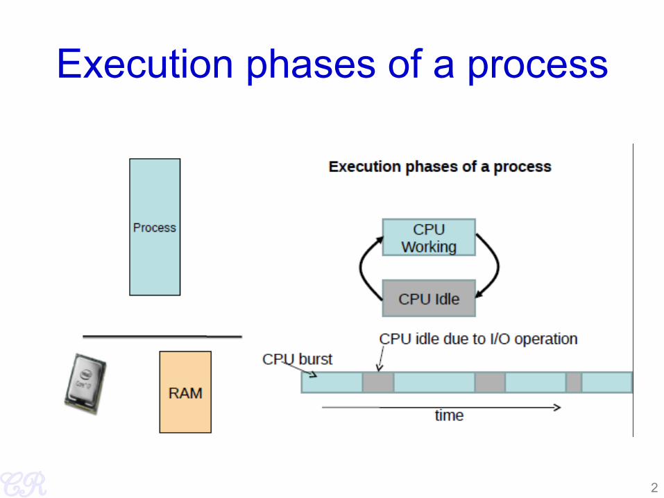
Execution phases of a process
2
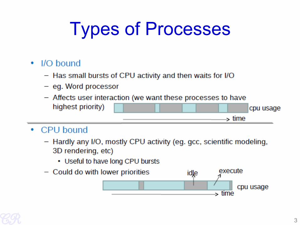
Types of Processes
3

CPU Scheduler
Scheduler triggered to run when timer interrupt occurs or when running process is blocked on I/O Scheduler picks another process from the ready queue Performs a context switch
Running Process
CPU Scheduler
Queue of Ready Processes
interrupt every 100ms
4
Schedulers
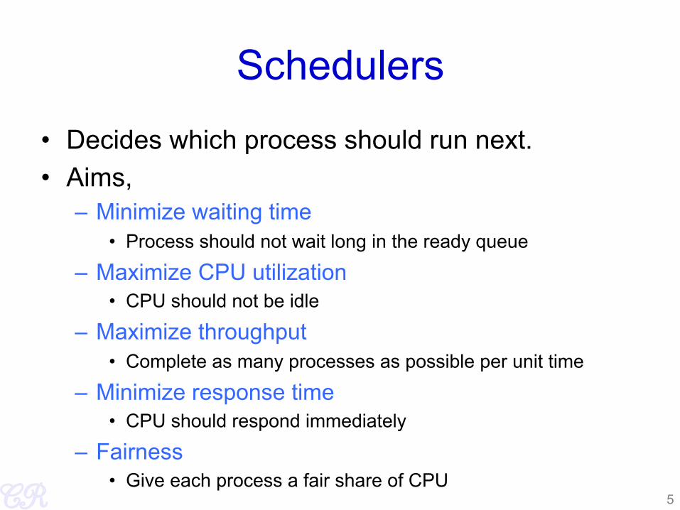
• Decides which process should run next. • Aims,
– Minimize waiting time • Process should not wait long in the ready queue
– Maximize CPU utilization • CPU should not be idle
– Maximize throughput • Complete as many processes as possible per unit time
– Minimize response time • CPU should respond immediately
– Fairness • Give each process a fair share of CPU
5
FCFS Scheduling (First Come First Serve)
• First job that requests the CPU gets the CPU • Non preemptive
– Process continues till the burst cycle ends
• Example
6
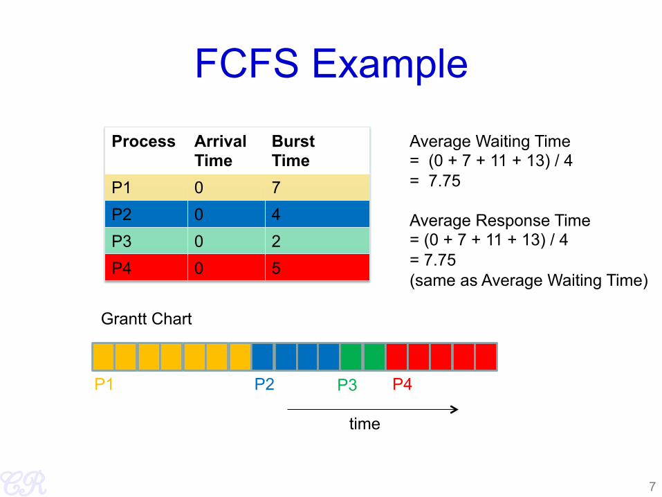
FCFS Example
Process Arrival Time
Burst Time
P1 0 7 P2 0 4 P3 0 2 P4 0 5
Grantt Chart
time
Average Waiting Time = (0 + 7 + 11 + 13) / 4 = 7.75 Average Response Time = (0 + 7 + 11 + 13) / 4 = 7.75 (same as Average Waiting Time)
P1 P2 P3 P4
7
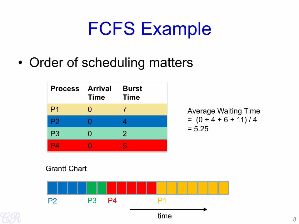
FCFS Example
• Order of scheduling matters
Process Arrival Time
Burst Time
P1 0 7 P2 0 4 P3 0 2 P4 0 5
Grantt Chart
time
Average Waiting Time = (0 + 4 + 6 + 11) / 4 = 5.25
P1 P2 P3 P4
8
FCFS Pros and Cons
• Advantages – Simple – Fair (as long as no process hogs the CPU, every
process will eventually run)
• Disadvantages – Waiting time depends on arrival order – short processes stuck waiting for long process to
complete
9
Shortest Job First (SJF) no preemption
• Schedule process with the shortest burst time – FCFS if same
• Advantages – Minimizes average wait time and average response
time • Disadvantages
– Not practical : difficult to predict burst time • Learning to predict future
– May starve long jobs
10
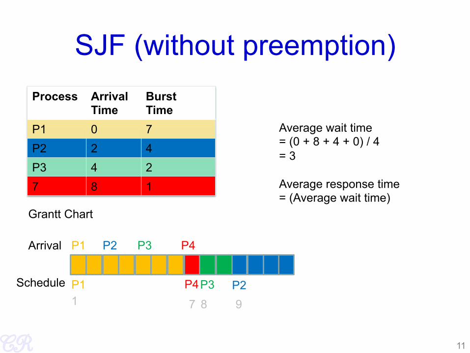
SJF (without preemption) Process Arrival
Time Burst Time
P1 0 7 P2 2 4 P3 4 2 7 8 1
Grantt Chart
P1 P2 P3 P4
P1 P2 P3 P4
Arrival
Schedule
Average wait time = (0 + 8 + 4 + 0) / 4 = 3 Average response time = (Average wait time)
11
1 7 8 9
Shortest Remaining Time First -- SRTF (SJF with preemption)
• If a new process arrives with a shorter burst time than remaining of current process then schedule new process
• Further reduces average waiting time and average response time
• Not practical
12
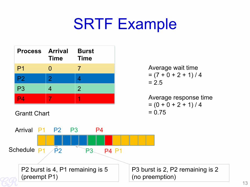
SRTF Example Process Arrival
Time Burst Time
P1 0 7 P2 2 4 P3 4 2 P4 7 1
Grantt Chart
P1 P2 P3 P4
P1 P2 P3
Arrival
Schedule
Average wait time = (7 + 0 + 2 + 1) / 4 = 2.5 Average response time = (0 + 0 + 2 + 1) / 4 = 0.75
P2 burst is 4, P1 remaining is 5 (preempt P1)
P3 burst is 2, P2 remaining is 2 (no preemption)
13
P4 P1

Round Robin Scheduling
• Run process for a time slice then move to FIFO
14
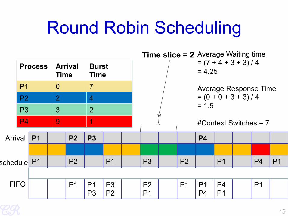
Round Robin Scheduling
Process Arrival Time
Burst Time
P1 0 7 P2 2 4 P3 3 2 P4 9 1
P1 P2 P3 P4
P1 P2 P1 P3 P2 P1 P4 P1
P1 P1 P3
P3 P2
P2 P1
P1 P1 P4
P4 P1
P1
Arrival
schedule
FIFO
Average Waiting time = (7 + 4 + 3 + 3) / 4 = 4.25 Average Response Time = (0 + 0 + 3 + 3) / 4 = 1.5 #Context Switches = 7
Time slice = 2
15
16
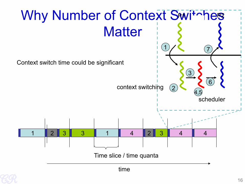
Why Number of Context Switches Matter
1 2 3 4 1 2 3 4 4
Time slice / time quanta
time
context switching
P1 P2
scheduler
1
2
3
4,5
6
7
3
Context switch time could be significant

Recall Context Switching Overheads
• Direct Factors affecting context switching time – Timer Interrupt latency – Saving/restoring contexts – Finding the next process to execute
• Indirect factors – TLB needs to be reloaded – Loss of cache locality (therefore more cache misses) – Processor pipeline flush
17
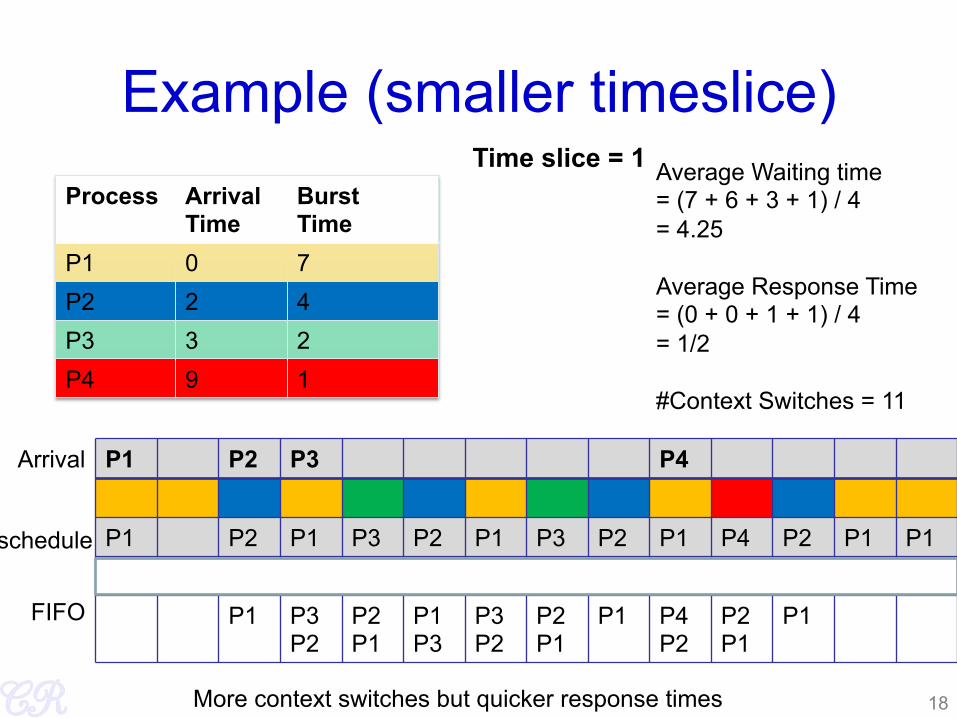
Example (smaller timeslice) Process Arrival
Time Burst Time
P1 0 7 P2 2 4 P3 3 2 P4 9 1
P1 P2 P3 P4
P1 P2 P1 P3 P2 P1 P3 P2 P1 P4 P2 P1 P1
P1 P3 P2
P2 P1
P1 P3
P3 P2
P2 P1
P1 P4 P2
P2 P1
P1
Arrival
schedule
FIFO
Average Waiting time = (7 + 6 + 3 + 1) / 4 = 4.25 Average Response Time = (0 + 0 + 1 + 1) / 4 = 1/2 #Context Switches = 11
Time slice = 1
18 More context switches but quicker response times
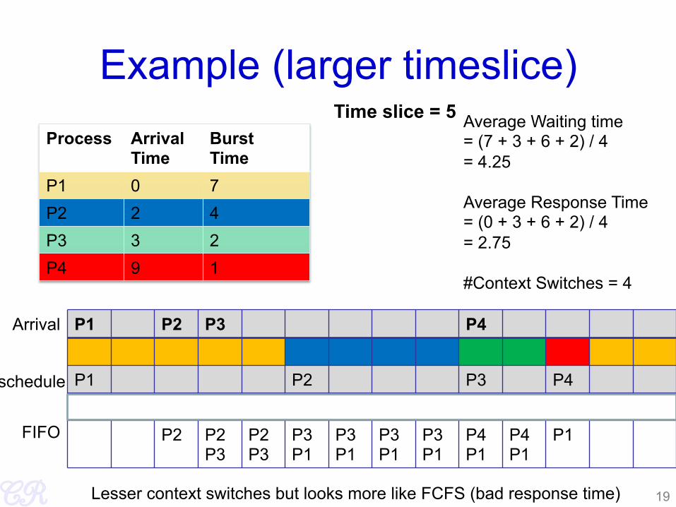
Example (larger timeslice) Process Arrival
Time Burst Time
P1 0 7 P2 2 4 P3 3 2 P4 9 1
P1 P2 P3 P4
P1 P2 P3 P4
P2 P2 P3
P2 P3
P3 P1
P3 P1
P3 P1
P3 P1
P4 P1
P4 P1
P1
Arrival
schedule
FIFO
Average Waiting time = (7 + 3 + 6 + 2) / 4 = 4.25 Average Response Time = (0 + 3 + 6 + 2) / 4 = 2.75 #Context Switches = 4
Time slice = 5
19 Lesser context switches but looks more like FCFS (bad response time)
Round Robin Scheduling
• Advantages – Fair (Each process gets a fair chance to run on the
CPU) – Low average wait time, when burst times vary – Faster response time
• Disadvantages – Increased context switching
• Context switches are overheads!!!
– High average wait time, when burst times have equal lengths
20

xv6 Scheduler Policy Decided by the Scheduling Policy
21
The xv6 schedule Policy --- Strawman Scheduler • organize processes in a list • pick the first one that
is runnable • put suspended task the
end of the list Far from ideal!! • only round robin scheduling policy • does not support priorities

Priority Based Scheduling Algorithms
22
Chester Rebeiro IIT Madras
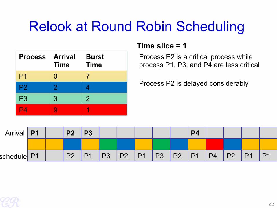
Relook at Round Robin Scheduling
Process Arrival Time
Burst Time
P1 0 7 P2 2 4 P3 3 2 P4 9 1
P1 P2 P3 P4
P1 P2 P1 P3 P2 P1 P3 P2 P1 P4 P2 P1 P1
Arrival
schedule
Time slice = 1
23
Process P2 is a critical process while process P1, P3, and P4 are less critical
Process P2 is delayed considerably
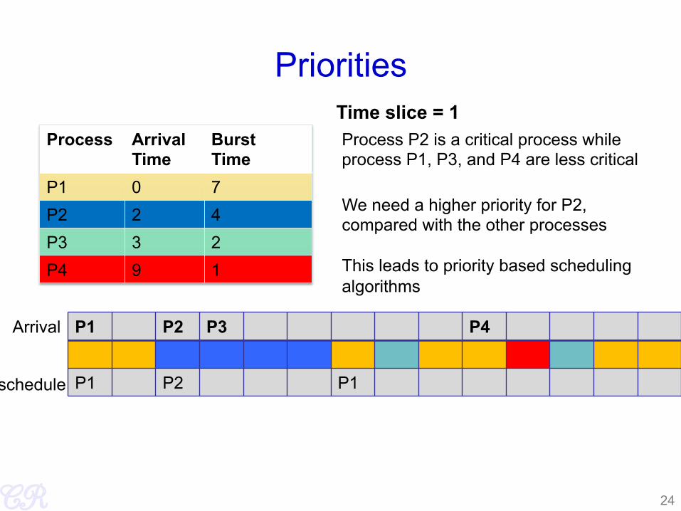
Priorities
Process Arrival Time
Burst Time
P1 0 7 P2 2 4 P3 3 2 P4 9 1
P1 P2 P3 P4
P1 P2 P1
Arrival
schedule
Time slice = 1
24
Process P2 is a critical process while process P1, P3, and P4 are less critical
We need a higher priority for P2, compared with the other processes This leads to priority based scheduling algorithms
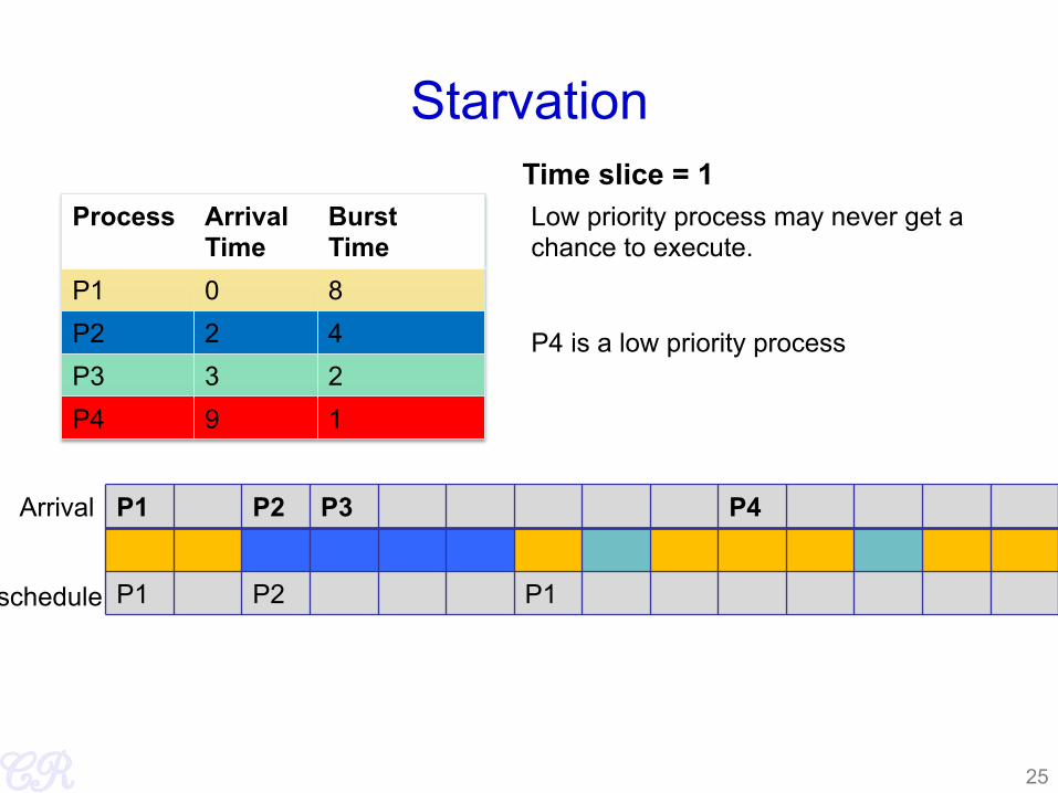
Starvation
Process Arrival Time
Burst Time
P1 0 8 P2 2 4 P3 3 2 P4 9 1
P1 P2 P3 P4
P1 P2 P1
Arrival
schedule
Time slice = 1
25
Low priority process may never get a chance to execute. P4 is a low priority process
Priority based Scheduling • Priority based Scheduling
– Each process is assigned a priority • A priority is a number in a range (for instance between 0 and 255) • A small number would mean high priority while a large number would mean
low priority
– Scheduling policy : pick the process in the ready queue having the highest priority
– Advantage : mechanism to provide relative importance to processes
– Disadvantage : could lead to starvation of low priority processes
26

Dealing with Starvation • Scheduler adjusts priority of processes to ensure that
they all eventually execute • Several techniques possible. For example,
– Every process is given a base priority – After every time slot increment the priority of all other process
• This ensures that even a low priority process will eventually execute
– After a process executes, its priority is reset
27
Priorities are of two types • Static priority : typically set at start of execution
– If not set by user, there is a default value (base priority)
• Dynamic priority : scheduler can change the process priority during execution in order to achieve scheduling goals – eg1. decrease priority of a process to give another process a
chance to execute – eg.2. increase priority for I/O bound processes
28
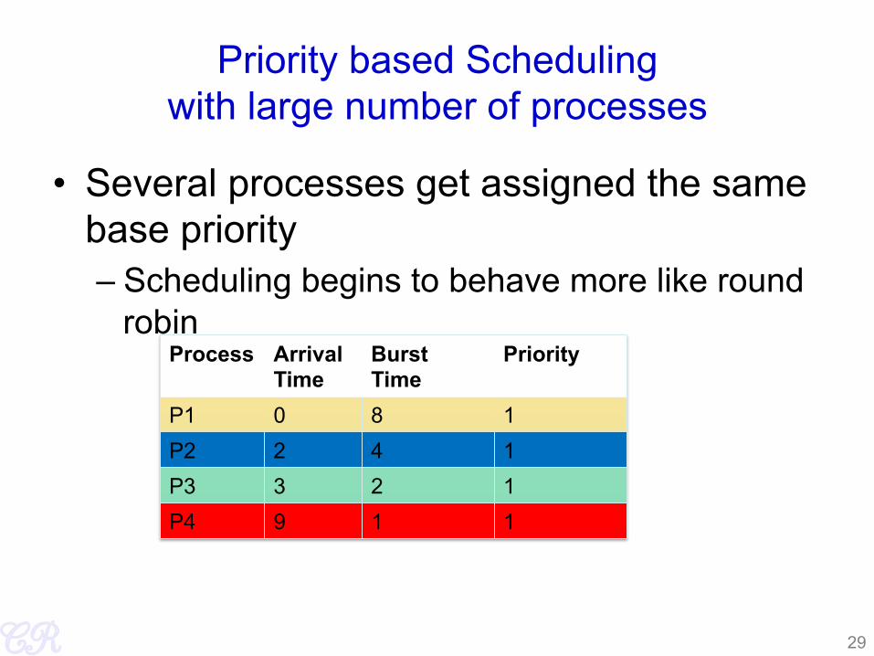
Priority based Scheduling with large number of processes
• Several processes get assigned the same base priority – Scheduling begins to behave more like round
robin
29
Process Arrival Time
Burst Time
Priority
P1 0 8 1 P2 2 4 1 P3 3 2 1 P4 9 1 1
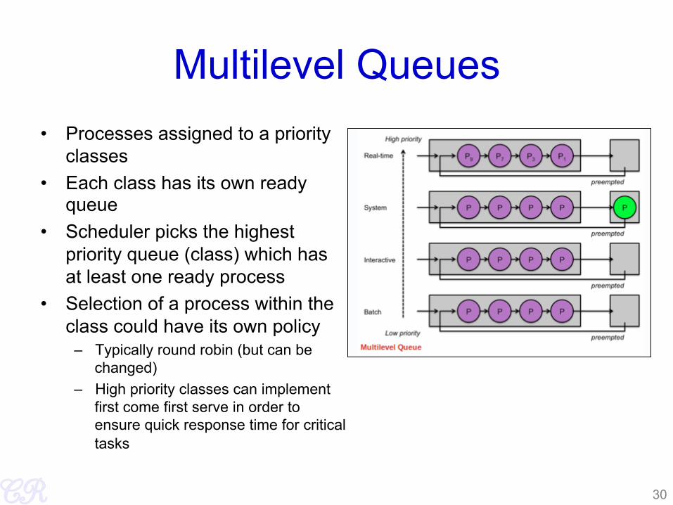
Multilevel Queues • Processes assigned to a priority
classes • Each class has its own ready
queue • Scheduler picks the highest
priority queue (class) which has at least one ready process
• Selection of a process within the class could have its own policy
– Typically round robin (but can be changed)
– High priority classes can implement first come first serve in order to ensure quick response time for critical tasks
30
More on Multilevel Queues
• Scheduler can adjust time slice based on the queue class picked – I/O bound process can be assigned to higher priority
classes with longer time slice – CPU bound processes can be assigned to lower
priority classes with shorter time slices • Disadvantage :
– Class of a process must be assigned apriori (not the most efficient way to do things!)
31
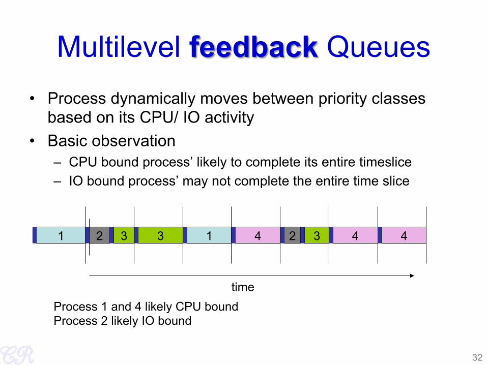
Multilevel feedback Queues • Process dynamically moves between priority classes
based on its CPU/ IO activity • Basic observation
– CPU bound process’ likely to complete its entire timeslice – IO bound process’ may not complete the entire time slice
32
1 2 3 4 1 2 3 4 4
time
3
Process 1 and 4 likely CPU bound Process 2 likely IO bound
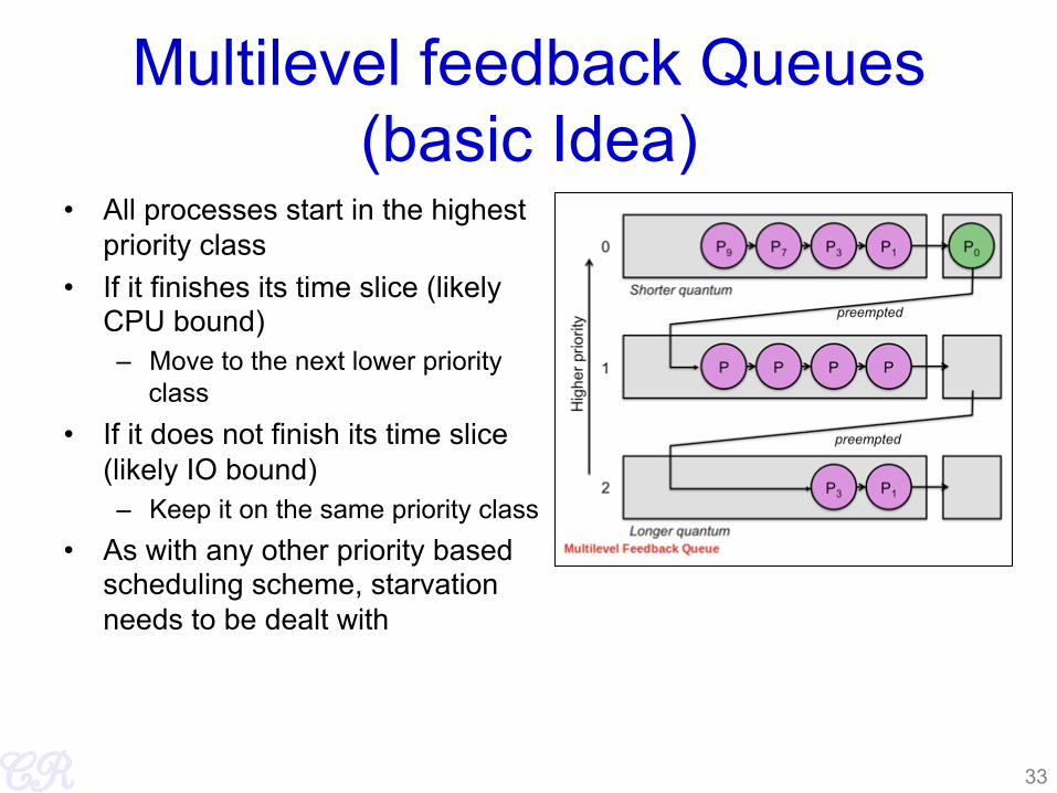
Multilevel feedback Queues (basic Idea)
• All processes start in the highest priority class
• If it finishes its time slice (likely CPU bound) – Move to the next lower priority
class • If it does not finish its time slice
(likely IO bound) – Keep it on the same priority class
• As with any other priority based scheduling scheme, starvation needs to be dealt with
33

Gaming the System
• A compute intensive process can trick the scheduler and remain in the high priority queue (class)
34
while(1){ do some work for most of the time slice sleep(till the end of the time slice) }
1 2 3 4 1 2 3 4 4
time
3
Process 4 is gaming the system
Sleep will force a context switch
35
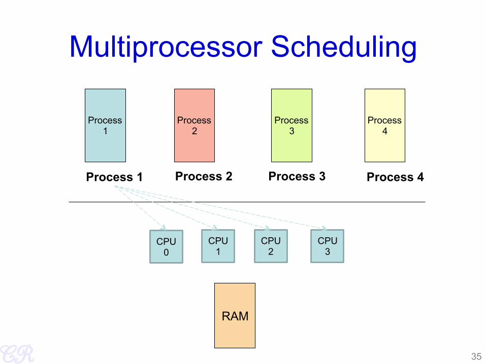
Multiprocessor Scheduling
RAM
Process 1 Process 2 Process 3 Process 4
Process 1
Process 2
Process 3
Process 4
CPU 0
CPU 1
CPU 2
CPU 3
Process Migration
• As a result of symmetrical multiprocessing – A process may execute in a processor in one
timeslice and another processor in the next time slice – This leads to process migration
• Migration is expensive, it requires all memories to be repopulated • Processor affinity
– Process has a bitmask that tells what processors it can run on
• Two types of processor affinity – Hard affinity – strict affinity to specific processors – Soft affinity
36
37
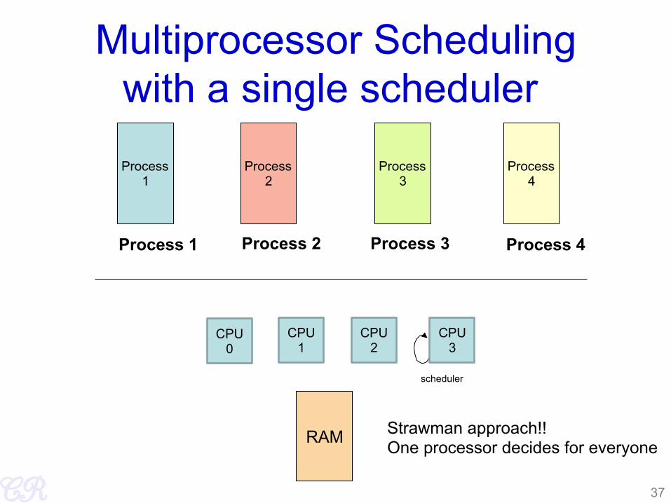
Multiprocessor Scheduling with a single scheduler
RAM
Process 1 Process 2 Process 3 Process 4
Process 1
Process 2
Process 3
Process 4
Strawman approach!! One processor decides for everyone
scheduler
CPU 0
CPU 1
CPU 2
CPU 3

38
Multiprocessor Scheduling (Symmetical Scheduling)
RAM
Process 1 Process 2 Process 3 Process 4
Process 1
Process 2
Process 3
Process 4
Each processor runs a scheduler independently to select the process to execute Requires locking to access the queues
scheduler scheduler scheduler scheduler
CPU 0
CPU 1
CPU 2
CPU 3
Two variants, • Global queues • Per CPU queues

Symmetrical Scheduling (with global queues)
39
Global queues of runnable processes
Advantages Good CPU Utilization Fair to all processes Disadvantages Not scalable (contention for the global queue) Processor affinity not easily achieved Locking needed in scheduler (not a good idea. Schedulers need to be highly efficient)
CPU 0
CPU 1
CPU 2
CPU 3
Used in Linux 2.4, xv6
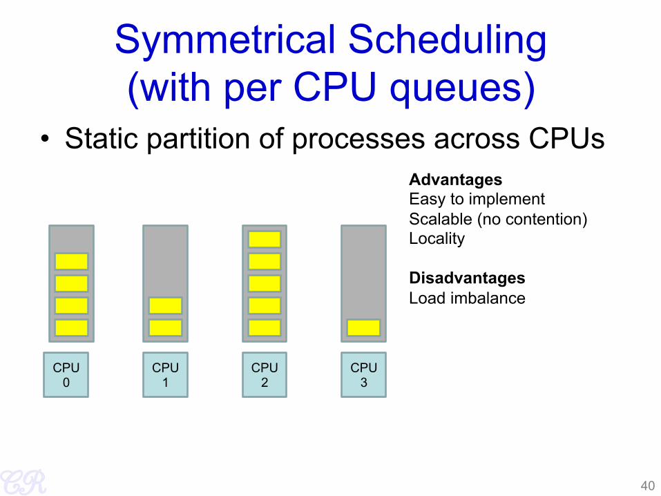
Symmetrical Scheduling (with per CPU queues)
• Static partition of processes across CPUs
40
CPU 0
CPU 1
CPU 2
CPU 3
Advantages Easy to implement Scalable (no contention) Locality Disadvantages Load imbalance
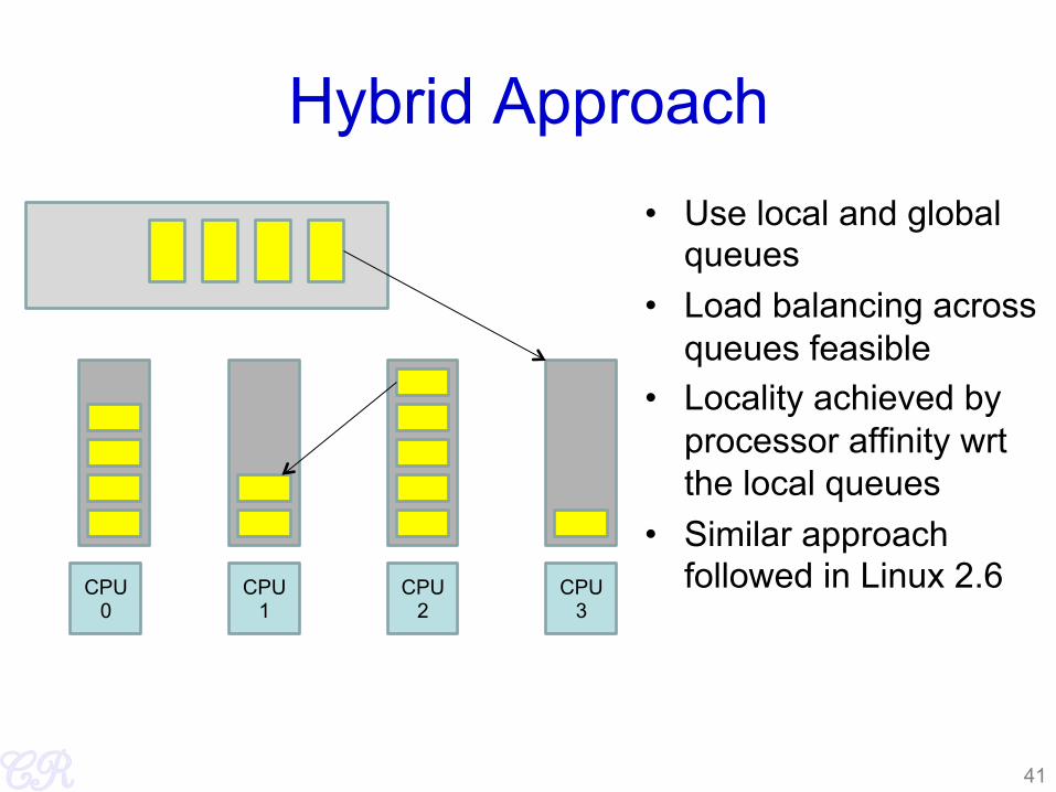
Hybrid Approach • Use local and global
queues • Load balancing across
queues feasible • Locality achieved by
processor affinity wrt the local queues
• Similar approach followed in Linux 2.6
41
CPU 0
CPU 1
CPU 2
CPU 3
Load Balancing
• On SMP systems, one processor may be overworked, while another underworked
• Load balancing attempts to keep the workload evenly distributed across all processors
• Two techniques – Push Migration : A special task periodically monitors
load of all processors, and redistributes work when it finds an imbalance
– Pull Migration : Idle processors pull a waiting task from a busy processor
42
Scheduling in Linux
Chester Rebeiro IIT Madras
Daniel P. Bovet and Marco Cesati, Understanding the Linux Kernel, 3rd Edition
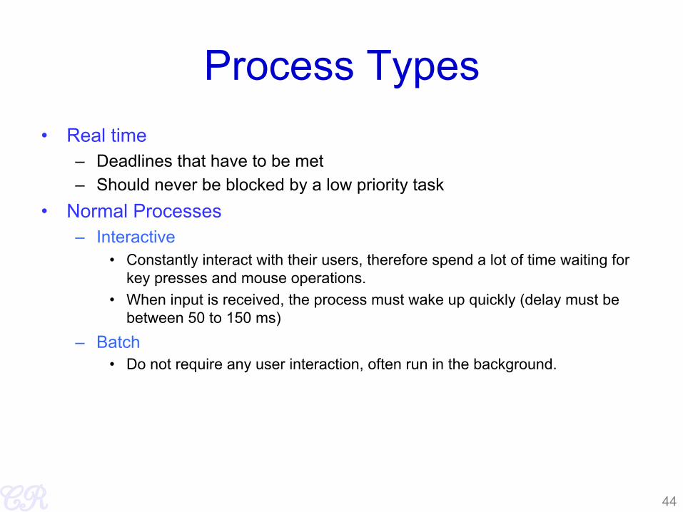
Process Types • Real time
– Deadlines that have to be met – Should never be blocked by a low priority task
• Normal Processes – Interactive
• Constantly interact with their users, therefore spend a lot of time waiting for key presses and mouse operations.
• When input is received, the process must wake up quickly (delay must be between 50 to 150 ms)
– Batch • Do not require any user interaction, often run in the background.
44
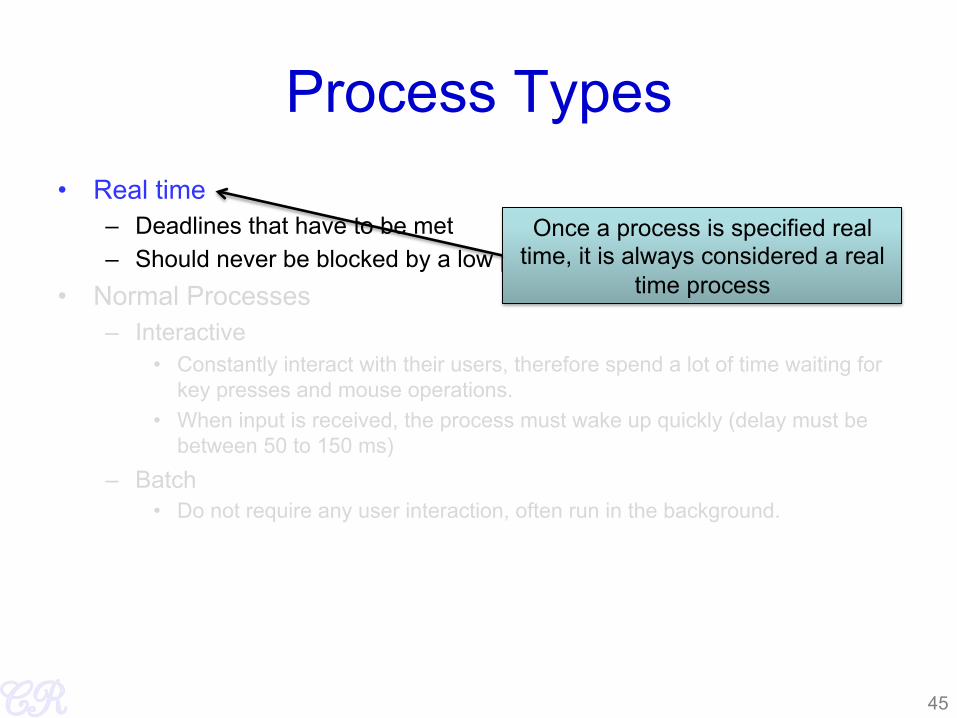
Process Types • Real time
– Deadlines that have to be met – Should never be blocked by a low priority task
• Normal Processes – Interactive
• Constantly interact with their users, therefore spend a lot of time waiting for key presses and mouse operations.
• When input is received, the process must wake up quickly (delay must be between 50 to 150 ms)
– Batch • Do not require any user interaction, often run in the background.
45
Once a process is specified real time, it is always considered a real
time process
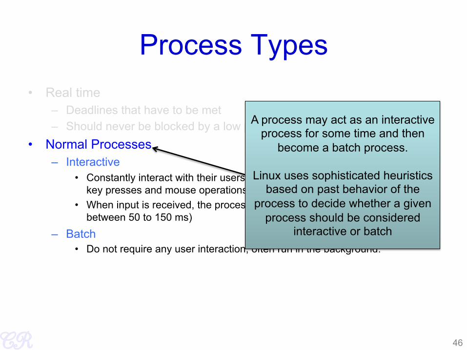
Process Types • Real time
– Deadlines that have to be met – Should never be blocked by a low priority task
• Normal Processes – Interactive
• Constantly interact with their users, therefore spend a lot of time waiting for key presses and mouse operations.
• When input is received, the process must wake up quickly (delay must be between 50 to 150 ms)
– Batch • Do not require any user interaction, often run in the background.
46
A process may act as an interactive process for some time and then
become a batch process.
Linux uses sophisticated heuristics based on past behavior of the
process to decide whether a given process should be considered
interactive or batch
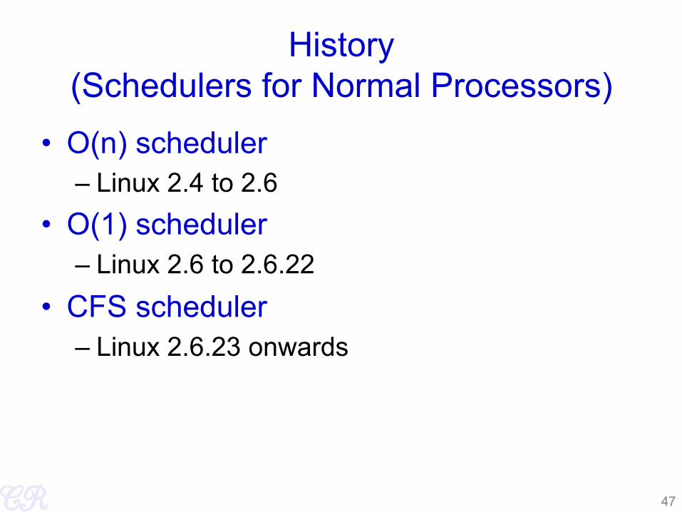
History (Schedulers for Normal Processors)
• O(n) scheduler – Linux 2.4 to 2.6
• O(1) scheduler – Linux 2.6 to 2.6.22
• CFS scheduler – Linux 2.6.23 onwards
47
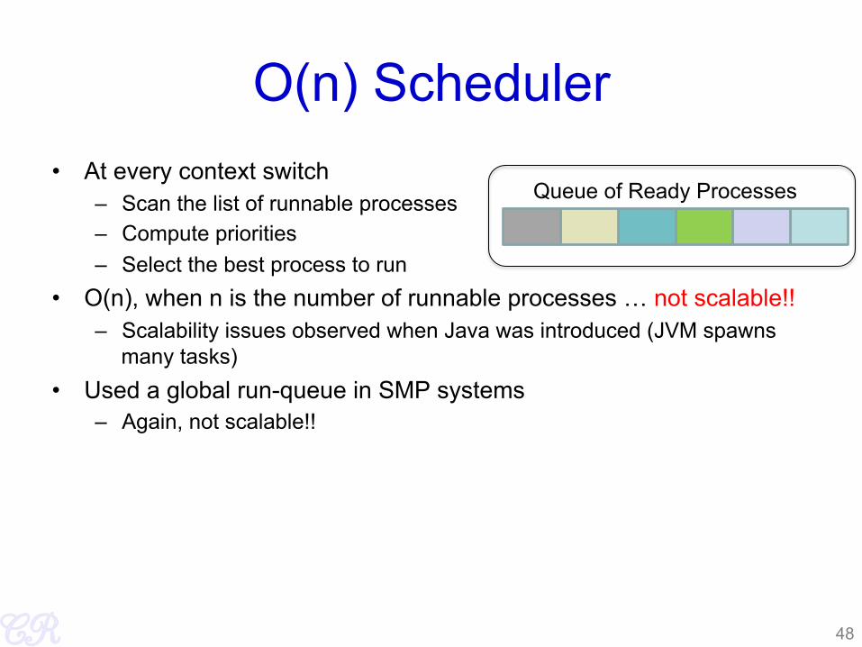
O(n) Scheduler • At every context switch
– Scan the list of runnable processes – Compute priorities – Select the best process to run
• O(n), when n is the number of runnable processes … not scalable!! – Scalability issues observed when Java was introduced (JVM spawns
many tasks) • Used a global run-queue in SMP systems
– Again, not scalable!!
48
Queue of Ready Processes
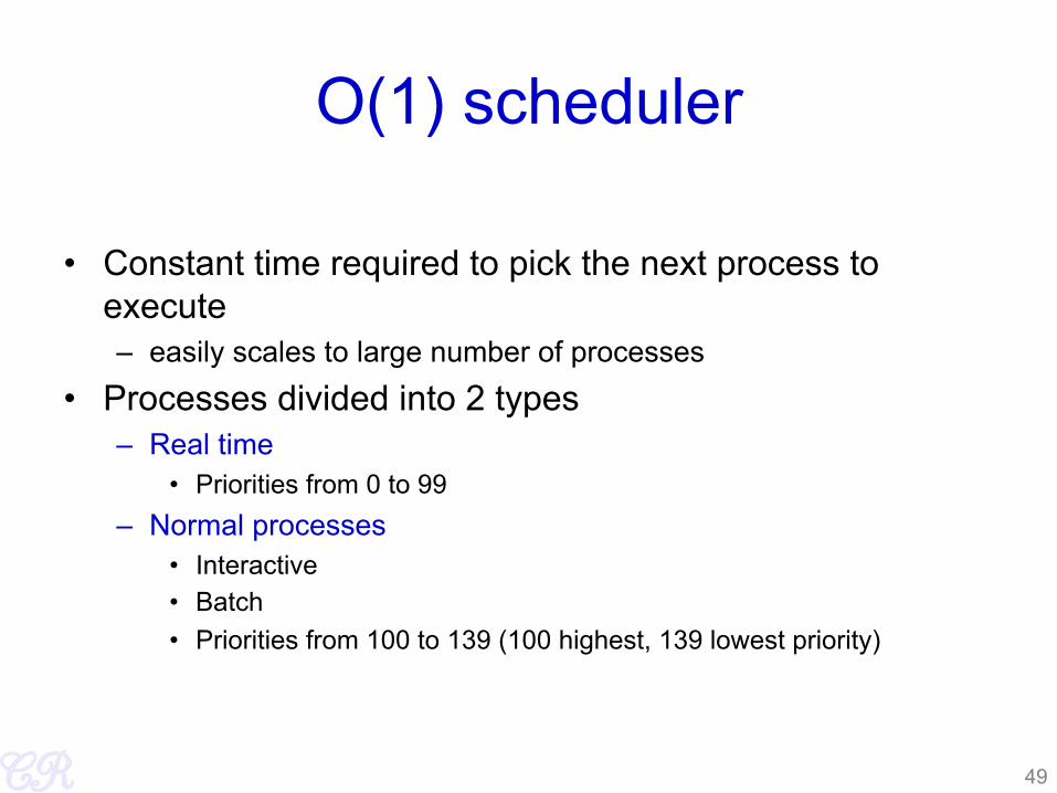
O(1) scheduler • Constant time required to pick the next process to
execute – easily scales to large number of processes
• Processes divided into 2 types – Real time
• Priorities from 0 to 99 – Normal processes
• Interactive • Batch • Priorities from 100 to 139 (100 highest, 139 lowest priority)
49
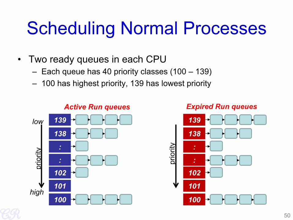
Scheduling Normal Processes • Two ready queues in each CPU
– Each queue has 40 priority classes (100 – 139) – 100 has highest priority, 139 has lowest priority
50
100
101
102 :
:
138
139
prio
rity
Active Run queues
100
101
102 :
:
138
139
Expired Run queues
prio
rity
low
high
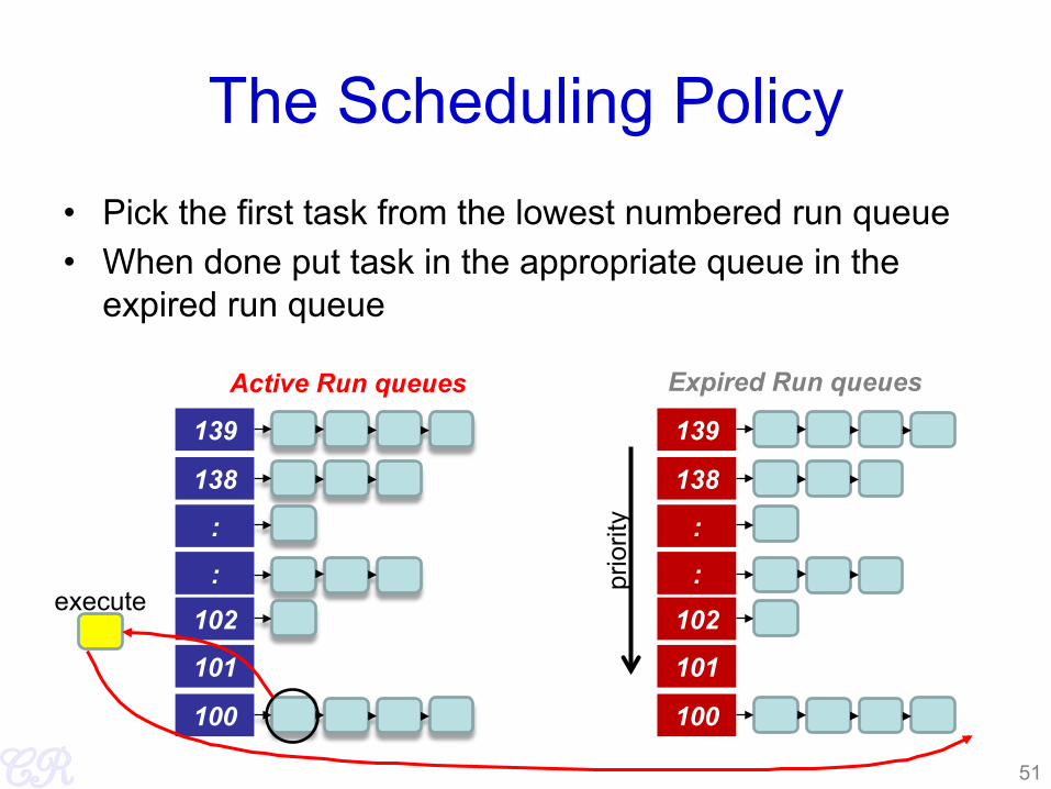
The Scheduling Policy • Pick the first task from the lowest numbered run queue • When done put task in the appropriate queue in the
expired run queue
51
100
101
102 :
:
138
139
Active Run queues
100
101
102 :
:
138
139
Expired Run queues
prio
rity
execute
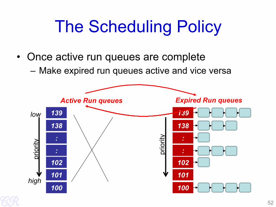
The Scheduling Policy
• Once active run queues are complete – Make expired run queues active and vice versa
52
100
101
102 :
:
138
139
prio
rity
Active Run queues
100
101
102 :
:
138
139
Expired Run queues
prio
rity
low
high
contant time? • There are 2 steps in the scheduling
1. Find the lowest numbered queue with at least 1 task 2. Choose the first task from that queue
• step 2 is obviously constant time • Is step 1 contant time?
• Store bitmap of run queues with non-zero entries • Use special instruction ‘find-first-bit-set’
– bsfl on intel
53
More on Priorities • 0 to 99 meant for real time processes • 100 is the highest priority for a normal process • 139 is the lowest priority • Static Priorities
– 120 is the base priority (default) – nice : command line to change default priority of a process $nice –n N ./a.out – N is a value from +19 to -20;
• most selfish ‘-20’; (I want to go first) • most generous ‘+19’; ( I will go last)
54
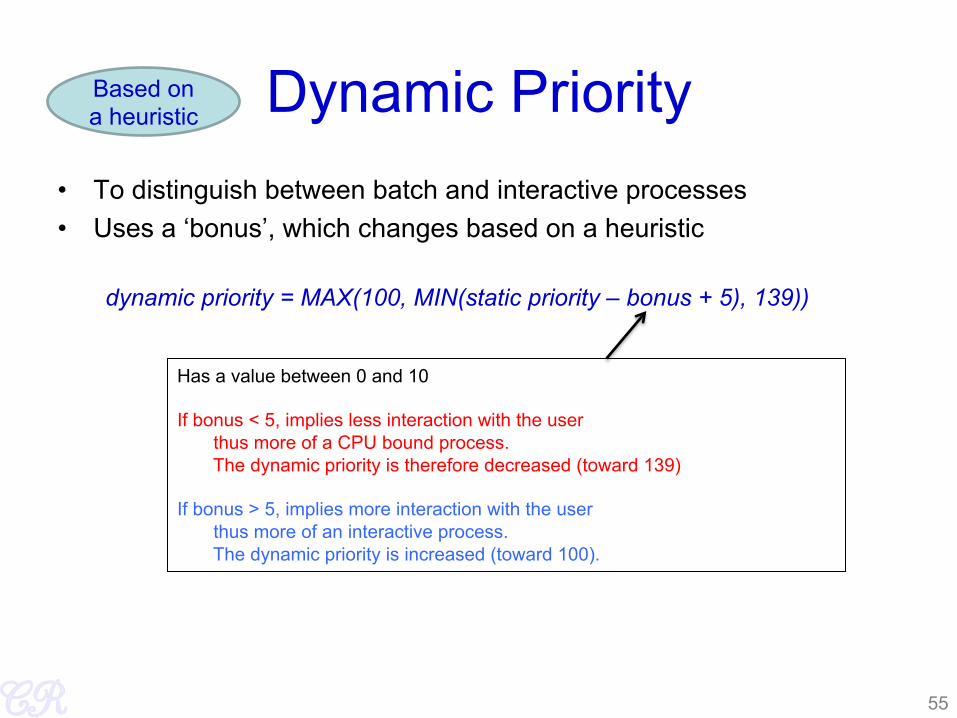
Dynamic Priority • To distinguish between batch and interactive processes • Uses a ‘bonus’, which changes based on a heuristic
dynamic priority = MAX(100, MIN(static priority – bonus + 5), 139))
55
Based on a heuristic
Has a value between 0 and 10 If bonus < 5, implies less interaction with the user thus more of a CPU bound process. The dynamic priority is therefore decreased (toward 139) If bonus > 5, implies more interaction with the user thus more of an interactive process. The dynamic priority is increased (toward 100).

Dynamic Priority (setting the bonus)
• To distinguish between batch and interactive processes • Based on average sleep time
– An I/O bound process will sleep more therefore should get a higher priority
– A CPU bound process will sleep less, therefore should get lower priority dynamic priority = MAX(100, MIN(static priority – bonus + 5), 139))
56

Dynamic Priority and Run Queues
• Dynamic priority used to determine which run queue to put the task
• No matter how ‘nice’ you are, you still need to wait on run queues --- prevents starvation
57
100
101
102 :
:
138
139
Active Run queues
100
101
102 :
:
138
139
Expired Run queues
execute
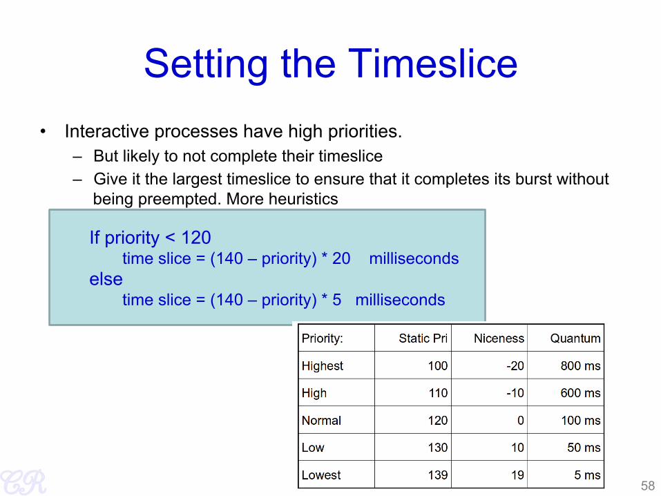
• Interactive processes have high priorities. – But likely to not complete their timeslice – Give it the largest timeslice to ensure that it completes its burst without
being preempted. More heuristics
If priority < 120 time slice = (140 – priority) * 20 milliseconds
else time slice = (140 – priority) * 5 milliseconds
Setting the Timeslice
58
Summarizing the O(1) Scheduler
• Multi level feed back queues with 40 priority classes
• Base priority set to 120 by default; modifiable by users using nice.
• Dynamic priority set by heuristics based on process’ sleep time
• Time slice interval for each process is set based on the dynamic priority
59
Limitations of O(1) Scheduler • Too complex heuristics to distinguish between interactive and non-
interactive processes • Dependence between timeslice and priority • Priority and timeslice values not uniform
60

Completely Fair Scheduling (CFS)
• The Linux scheduler since 2.6.23 • By Ingo Molnar
– based on the Rotating Staircase Deadline Scheduler (RSDL) by Con Kolivas.
– Incorporated in the Linux kernel since 2007 • No heuristics. • Elegant handling of I/O and CPU bound processes.
61
Completely Fair Scheduling (CFS)
62
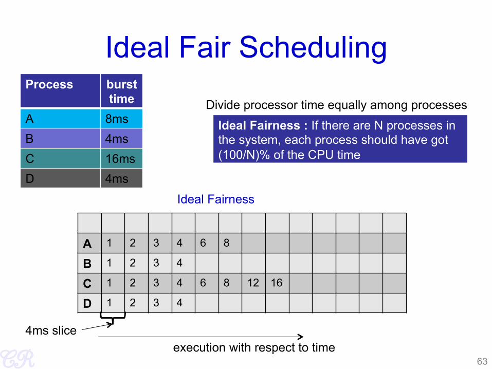
Ideal Fair Scheduling Process burst
time A 8ms B 4ms C 16ms D 4ms
63
Ideal Fairness : If there are N processes in the system, each process should have got (100/N)% of the CPU time
Ideal Fairness
A 1 2 3 4 6 8
B 1 2 3 4
C 1 2 3 4 6 8 12 16
D 1 2 3 4
4ms slice execution with respect to time
Divide processor time equally among processes

Ideal Fair Scheduling Process burst
time A 8ms B 4ms C 16ms D 4ms
64
Ideal Fairness : If there are N processes in the system, each process should have got (100/N)% of the CPU time
Ideal Fairness
A 1 2 3 4 6 8
B 1 2 3 4
C 1 2 3 4 6 8 12 16
D 1 2 3 4
4ms slice execution with respect to time
Divide processor time equally among processes
Each process gets 4/4 = 1ms of the processor time
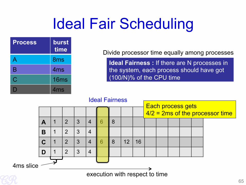
Ideal Fair Scheduling Process burst
time A 8ms B 4ms C 16ms D 4ms
65
Ideal Fairness : If there are N processes in the system, each process should have got (100/N)% of the CPU time
Ideal Fairness
A 1 2 3 4 6 8
B 1 2 3 4
C 1 2 3 4 6 8 12 16
D 1 2 3 4
4ms slice execution with respect to time
Divide processor time equally among processes
Each process gets 4/2 = 2ms of the processor time

Ideal Fair Scheduling Process burst
time A 8ms B 4ms C 16ms D 4ms
66
Ideal Fairness : If there are N processes in the system, each process should have got (100/N)% of the CPU time
Ideal Fairness
A 1 2 3 4 6 8
B 1 2 3 4
C 1 2 3 4 6 8 12 16
D 1 2 3 4
4ms slice execution with respect to time
Divide processor time equally among processes
The single process gets the entire 4ms of the processor time
Virtual Runtimes
• With each runnable process is included a virtual runtime (vruntime) – At every scheduling point, if process has run
for t ms, then (vruntime += t) – vruntime for a process therefore
monotonically increases
67
The CFS Idea
• When timer interrupt occurs – Choose the task with the lowest vruntime
(min_vruntime) – Compute its dynamic timeslice – Program the high resolution timer with this timeslice
• The process begins to execute in the CPU • When interrupt occurs again
– Context switch if there is another task with a smaller runtime
68
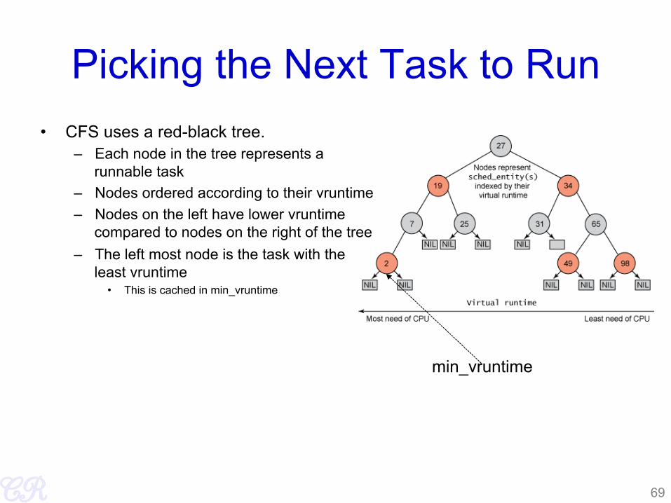
Picking the Next Task to Run • CFS uses a red-black tree.
– Each node in the tree represents a runnable task
– Nodes ordered according to their vruntime – Nodes on the left have lower vruntime
compared to nodes on the right of the tree – The left most node is the task with the
least vruntime • This is cached in min_vruntime
69
min_vruntime

Picking the Next Task to Run • At a context switch,
– Pick the left most node of the tree • This has the lowest runtime. • It is cached in min_vruntime. Therefore
accessed in O(1) – If the previous process is runnable, it is
inserted into the tree depending on its new vruntime. Done in O(log(n))
• Tasks move from left to right of tree after its execution completes… starvation avoided
70
min_vruntime
Why Red Black Tree?
• Self Balancing – No path in the tree will be twice as long as any other path
• All operations are O(log n) – Thus inserting / deleting tasks from the tree is quick and efficient
71
Priorities and CFS • Priority (due to nice values) used to weigh the vruntime
• if process has run for t ms, then vruntime += t * (weight based on nice of process)
• A lower priority implies time moves at a faster rate compared to that of a high priority task
72
I/O and CPU bound processes
• What we need, – I/O bound should get higher priority and get a longer
time to execute compared to CPU bound – CFS achieves this efficiently
• I/O bound processes have small CPU bursts therefore will have a low vruntime. They would appear towards the left of the tree…. Thus are given higher priorities
• I/O bound processes will typically have larger time slices, because they have smaller vruntime
73
New Process
• Gets added to the RB-tree • Starts with an initial value of
min_vruntime.. • This ensures that it gets to execute quickly
74

Thank You
75