IOSCO Report: Leverage

Consultation Paper

The Board OF THE

INTERNATIONAL ORGANIZATION OF SECURITIES COMMISSIONS CR08/2018 NOVEMBER 2018

This paper is for public consultation purposes only. It has not been approved for any

other purpose by the IOSCO Board or any of its members.

ii

Copies of publications are available from: The International Organization of Securities Commissions website www.iosco.org

© International Organization of Securities Commissions 2018. All rights reserved. Brief excerpts may be reproduced or translated provided the source is stated.

iii

Foreword The Board of the International Organization of Securities Commissions (IOSCO) has published this Consultation Report to request feedback on a proposed framework to help assess leverage used by investment funds. The proposed framework comprises a two-step process aimed at achieving a meaningful and consistent assessment of global leverage, as part of an effort to address risks that may arise from certain asset management activities. How to Submit Comments Comments may be submitted by one of the three following methods on or before 1 February 2019. To help us process and review your comments more efficiently, please use only one method. Important: All comments will be made available publicly, unless anonymity is specifically requested. Comments will be converted to PDF format and posted on the IOSCO website. Personal identifying information will not be edited from submissions. 1. Email

• Send comments to consultation-08-2018@iosco.org. • The subject line of your message must indicate ‘IOSCO Report: Leverage.’ • If you attach a document, indicate the software used (e.g., WordPerfect, Microsoft

WORD, ASCII text, etc) to create the attachment. • Do not submit attachments as HTML, PDF, GIFG, TIFF, PIF, ZIP or EXE files.

2. Facsimile Transmission Send by facsimile transmission using the following fax number: + 34 (91) 555 93 68. 3. Paper Send 3 copies of your paper comment letter to: Dr Shane Worner International Organization of Securities Commissions (IOSCO) Calle Oquendo 12 28006 Madrid Spain Your comment letter should indicate prominently that it is a ‘Public Comment on IOSCO Report: Leverage.

iv

Contents

Chapter Page 1 Introduction 1 2 Step 1: Analysis of potential metrics 5 3 Articulation of one or more step 1 metrics with supplementary

data points 17

4 Step 2: Risk Analyses of Funds 19

5 Appendix A - Step 1 techniques: Calculation and reporting -

Gross Notional Measures framework analysis 21

6 Appendix B - Metrics not consulted on in this paper 27 7 Appendix C – Step 2 29

1

Chapter 1 – Introduction On January 12, 2017, the Financial Stability Board (FSB) issued a report, ‘Policy Recommendations to Address Structural Vulnerabilities from Asset Management Activities’1. The report provides policy recommendations to address risks to global financial stability associated with certain potential structural vulnerabilities which may result from asset management activities. The report includes recommendations related to the use of leverage in investment funds addressed to IOSCO.

The use of leverage by investment funds brings with it potential risks to both investors and financial markets: while leverage may amplify investment fund returns, it can also amplify losses. The use of leverage may also, in certain circumstances, impair the proper functioning of markets via different contagion channels (as referred to in the above-mentioned FSB report). Securities regulators, in accordance with their respective mandates, therefore have an interest in monitoring the use of leverage by funds.

In Recommendation 10 of its report, the FSB asked IOSCO to “identify and or develop consistent measures of leverage in funds to facilitate more meaningful monitoring of leverage for financial stability purposes, and help enable direct comparisons across funds and at a global level. IOSCO should also consider identifying and/or developing more risk-based measure(s) to complement the initial measures with a view to enhance authorities’ understanding and monitoring of risks that leverage in funds may create. In both cases, IOSCO should consider appropriate netting and hedging assumptions and where relevant build on existing measures.” In addition, two other recommendations complete the FSB’s recommendations on leverage, as detailed in the FSB report2. This paper focuses on recommendation 10 only. This consultation paper, drafted in consultation with FSB members and following initial discussions with market participants3, responds to Recommendation 10 by outlining a proposed framework that could facilitate regulators calculating and analysing leverage in funds over time in a sufficiently consistent manner across jurisdictions. This would be carried out in two steps. The first step would use the measures of leverage identified and/or developed, with a view to identify and analyse funds that may pose a risk to financial stability. Step 2 would involve further analysis of this sub-set of funds, as described below.

Ø The goal of step 1 is to provide regulators with a means of efficiently excluding from consideration funds that are unlikely to pose risks to the financial system and so do not warrant further analysis. The first step of this process, described in chapter 2 below,

1 Policy Recommendations to Address Structural Vulnerabilities from Asset Management Activities, FSB.

12 January 2017, available at: http://www.fsb.org/wp-content/uploads/FSB-Policy-Recommendations-on-Asset-Management-Structural-Vulnerabilities.pdf

2 FSB Recommendation 11 is directed to national authorities and read as follows: ‘Authorities should collect data on leverage in funds, monitor the use of leverage by funds not subject to leverage limits or which may pose significant leverage-related risks to the financial system, and take action when appropriate.’

FSB Recommendation 12 is contingent on the completion of the current work on Recommendation 10. Recommendation 12 reads as follows: ‘IOSCO should collect national/regional aggregated data on leverage across its member jurisdictions based on the consistent measures it develops.’

3 IOSCO organised two industry workshops in Paris and Washington DC with a range of asset managers and investment banks which provide leverage to investment funds.

2

discusses how regulators could identify which funds may pose leverage-related financial stability risks. Step 1 provides an approach to how regulators could use exposure metrics in various contexts and situations complemented by additional information, to filter and select a subset of investment funds for further analysis.

Ø The second step then focuses on risk-based analysis on the subset of funds identified in step 1. Given that some risk-based or other measures or analyses are appropriate for some funds and not for others, depending on their characteristics and investment strategies, it is up to each jurisdiction to determine the most appropriate risk assessment to undertake. IOSCO does not prescribe a particular set of metrics or other analytical tools. Some illustrative specific cases and applicable measures are detailed under Appendix C, as examples of analysis that jurisdictions could, to the extent relevant, consider.

In consulting in this way, it is acknowledged that there is an underlying tension between achieving precise leverage measures and arriving at sufficiently simple, robust metrics that can be applied in a consistent manner to the wide range of funds offered in different jurisdictions. While the two-step framework seeks an appropriate balance, consistent with the FSB report, it also (i) addresses synthetic leverage, by including exposure created by derivatives; (ii) considers different approaches to analysing netting and hedging and the directionality of positions; and (iii) includes approaches that limit model risk.

The present consultation focuses mainly on the first step. It also invites feedback on the second step as well as the articulation of the two-step approach. This is an iterative process within which the longer-term goal of achieving a meaningful consistent assessment of global leverage can be met while taking into account the different stages of development and sophistication of markets around the world. A number of jurisdictions have well developed systems for calculating, collecting and analysing information related to fund leverage, which generally is provided to them by asset managers including alternative asset managers. However, this is by no means the case for all jurisdictions. In the absence of an existing framework, IOSCO encourages regulators to look to this work to inform any initiatives related to establishing their own measurement processes.

What is leverage?

Leverage is a financial technique generally used to increase investment exposure. Leverage allows a fund to increase its potential gains, as well as losses, by using financial instruments and/or borrowed money to increase the fund’s market exposure beyond its net asset value. Leverage can come in a variety of different forms, for example, debt or some types of derivatives when used for this purpose.

Leverage in investment funds is typically expressed as a ratio of the fund’s market exposure (however defined) over its net asset value.

Leverage = market exposure

net asset value

Measures of market exposure can capture investment exposure taken both through derivatives and borrowed money. Although derivatives can be used to amplify the risk and potential returns in a fund’s portfolio, they are also routinely used for other purposes, including:

3

- hedging risks; - enhancing liquidity in situation where derivatives are more liquid than their

underlying reference assets; - improving transactional efficiency; - gaining exposure to less accessible markets; - cash management, and - adjusting the characteristics of the fund’s portfolio, such as the portfolio’s duration, or

sensitivity to changes in credit spreads and/or interest rates term structure.

A fund’s use of derivatives alone – which can increase certain measures of market exposure - should not, therefore, be seen as solely synonymous with the amplification of risk and returns.

Challenges in measuring leverage

Rules relating to leverage in funds and its measurement and monitoring vary across jurisdictions around the world. Where metrics are in place they may not be easily comparable as different jurisdictions have developed differing metrics. There are also challenges regarding how leverage, both on and off-balance sheet, is captured by different metrics4. Comparability is also hampered by the wide variety of funds and fund strategies offered around the world: measures of fund leverage that are appropriate for one type of fund or fund strategy may be less appropriate, or informative, if applied to other types of funds or strategies.

The availability of the data required to measure leverage also presents challenges. While some jurisdictions, notably the United States and European Union member states, require detailed reporting on leverage metrics5, (including data points sufficient to calculate leverage metrics), others do not. This leads to potential data gaps in relation to the extent of leverage in funds or the lack of it. Identifying which funds and which group of funds do not make substantial use of leverage will better focus regulatory resources on those funds that do.

As noted above, the details of regulatory disclosures and reporting requirements vary. This reflects differences in regulatory frameworks which may be tailored to local markets. While this may be appropriate for those markets, it does create challenges for the comparability of leverage data.

These considerations highlight the inherent tension between the ability of a given metric to provide accurate and precise information and the need for measurement to be as clear and comparable as possible. The interpretation of data is further complicated given that derivatives, which can increase measures of a fund’s market exposure, may reflect the use of hedging or cost-efficiency techniques, and not just the amplification of potential risk and returns.

However, while we note the challenges described above, collection, aggregation and analysis of available data does already take place to a certain extent under the IOSCO Hedge Fund Survey. While we acknowledge the more limited scope and data limitations of the survey, it 4 Jurisdictions that collect significant leverage-related data also may not collect data, or the same data,

from all funds in the relevant jurisdiction. There is thus variability in the data available both across jurisdictions and within jurisdictions across different types of funds.

5 See, e.g., Form PF, a reporting form applicable to certain investment advisers registered with the U.S. Securities and Exchange Commission or in the EU, the AIFMD reporting requirements applicable to alternative investment managers and which include information on managers and the alternative investment funds they manage.

4

provides a reference point over time for the extent of leverage used by certain investment funds in participating jurisdictions6. We also highlight that the jurisdictions overseeing the largest fund markets currently require regular reporting of leverage metrics. Although the details of these metrics are not identical, there is substantial overlap in the types of information covered. The two-step approach could therefore build on existing measures while facilitating collaboration among regulators across these jurisdictions.

6 IOSCO Survey of Hedge Funds 2017 used data provided by the AMF (France), BaFin (Germany),

Central Bank of Ireland, CSSF (Luxembourg), FCA (UK), MAS (Singapore), SEC (United States) and SFC (Hong Kong), and input from the Cayman Islands Monetary Authority.

5

Chapter 2 – Step 1: Analysis of potential metrics

There is a range of metrics available to measure leverage within investment funds. In this chapter, we consult on three metrics to assess whether they may be effective, including in combination with each other and other information, as part of first step of the proposed two-step approach.

In selecting the metrics to consult on in this paper, we have borne the following factors in mind. The metrics should as far as possible:

• be able to be applied across all strategies and methods of leverage used by funds across jurisdictions;

• avoid model risk; • facilitate the identification of funds which may pose a risk to financial stability.

Taking these criteria into consideration—and the advantages of metrics that are relatively easy to calculate using simple data points—the metrics that follow are based on notional exposure. We recognise that, used in isolation, the methodologies discussed below do not necessarily provide all of the information necessary to allow one securities regulator, depending on the sophistication of its market and information already made available to it, to filter funds and identify those with potential leverage-related risks as part of step 1. They may prove more meaningful information when used in combination with each other. IOSCO also assessed other methodologies which do not appear to be appropriate for the purposes of the work undertaken by IOSCO. The methodologies not selected are described in Appendix B together with their respective strengths and weaknesses.

1. Gross Notional Exposure (GNE) without adjustment

This metric represents the gross market exposure of a fund which is calculated by summing the absolutes values of the notional amounts of a fund’s derivatives and the value of the fund’s other investments7. No adjustments are made to any of the values.

This metric has some advantages as part of the two-step process: it is relatively easy to calculate and apply on a reasonably consistent basis across different types of funds using simple data points, and it avoids model risk. This metric provides information about a fund’s market footprint. A high measure indicates that a fund may be taking on high levels of leverage. However, such a figure may also show that a fund is using derivatives extensively, without being able to identify whether derivatives have been used for purposes other than obtaining leverage, such as those noted above. Fund managers that would otherwise use derivatives for

7 The term “notional amount” is used differently by different people in different contexts. In this

consultation paper the term generally refers to the market value of an equivalent position in the derivative’s underlying reference asset, or the principal amount on which payment obligations under the derivative are based. We believe this is consistent with market practice. Many funds today report notional amounts in regulatory filings. See, e.g., Form PF, General Instruction 15; Section 2b, Item B, Question 30 (requiring advisers to report the “value” of the exposures of each qualifying hedge fund; defining “value” for purposes of derivatives as gross notional value); CESR, Consultation Paper, Guidelines on Risk Measurement and the Calculation of Global Exposure and Counterparty Risk for UCITS (Apr. 19, 2010), at Section 2.1 (setting out proposed guidelines on the conversion of financial derivatives into the equivalent position in the underlying assets of those derivatives).

6

purposes other than obtaining leverage could be incentivised to use other, potentially more costly and less efficient methods if there were a concern about having a high GNE. The limitations of this metric include:

• it does not reflect the fact that a fund could be using derivatives for hedging or other purposes8;

• its unadjusted nature may overstate a fund’s exposure, particularly when the fund uses short-term interest rate derivatives and options9;

• it does not differentiate between exposures to different asset classes. For example, two given funds with the same gross exposure are treated the same even if one fund’s exposure is to more volatile assets, such as equities or commodities, and the other’s exposure is to less volatile assets, such as short-term interest rate contracts;

• if multiple funds’ gross exposures were aggregated together, there is a risk that the aggregate figure also may present an incomplete, and potentially misleading, picture of the funds’ overall market exposure.

GNE is therefore a basic method of assessing leverage as it only provides a baseline measure of a fund’s market exposure and does not quantify the risks associated with different types of derivatives or the purpose for which they are being used. As a result, this metric tends to overstate a fund’s economic exposure and should be viewed as a very conservative measure of leverage.

Table [1]: Pros and Cons of Gross Notional Exposure Without Adjustments

PROS CONS Relatively easy to calculate and apply on a reasonably consistent basis across different types of funds

Can overstate exposure, particularly short-dated interest rate derivatives and options

Uses simple data points Does not account for netting or hedging relationships and may then overstate the extent to which a fund’s net asset value will change in response to market changes if the fund is using derivatives to hedge or otherwise reduce market exposure

Avoids model risk

Does not account for netting or hedging relationships and so exclude any risk of impairing comparability of metrics or undermining leverage

Does not differentiate between exposures to low-risk and high-risk assets

Tends to overstate leverage Source: IOSCO

8 Please see appendix A page 20 for further details. 9 The notional amount of an option, without a delta adjustment, may overstate the exposure the option

creates to the underlying reference asset. A measure that does not adjust interest rate derivatives may overstate a CIS’ exposure to interest rate changes.

7

2. Adjusted Gross Notional Exposure

A fund’s adjusted GNE is calculated in the same manner as described above but reflects adjustments for interest rate derivatives and options.

Interest rate derivatives can be adjusted in different ways:

• present interest rate derivatives’ notional amounts in terms of ten-year bond equivalents. We understand that many market participants analyse interest rate derivatives in terms of ten-year bond equivalents for risk management and other purposes. This adjustment can be done on the basis of the duration (or modified duration) of the interest rate derivative relative to the duration of a ten-year bond; or

• adjust the fund’s interest rate derivatives relative to the fund’s target duration, for funds that have target durations.

Presenting interest rate derivatives as ten-year bond equivalents allows the comparison of different interest rate derivatives that provide similar exposure to changes in interest rates but that have different unadjusted notional amounts. Expressing interest rate derivatives as ten-year bond equivalents similarly addresses the concern that short-term interest rate derivatives in particular can produce large unadjusted notional amounts that may not correspond to large exposures to interest rate changes.

Delta adjusting options similarly is designed to provide for a more tailored notional amount that better reflects the exposure that an option creates to the underlying reference asset10. Market participants similarly consider options’ deltas for risk management, hedging, and other purposes.

Adjusted GNE generally shares the same advantages and disadvantages of GNE as discussed above. However, Adjusted GNE attempts to limit the overstatement of a fund’s exposure to interest rate derivatives and options.

Table [2]: Pros and Cons of Adjusted Gross Notional Exposure

PROS CONS Attempts to risk adjust interest rate derivatives and options exposures

Can still overstate exposure to interest rate derivatives and options although to a lesser extent than GNE

Relatively easy to calculate and apply on a reasonably consistent basis across different types of funds

Does not account for netting or hedging relationships and may then overstate the extent to which a fund’s net asset value will change in response to market changes if the fund is using derivatives to hedge or otherwise reduce market exposure

Uses simple data points

Avoids model risk Does not differentiate between exposures to low-risk and high-risk assets

10 Take, for example, a fund that sells an at-the-money call option on a particular security with a notional

amount of $100. If the delta of this option is -0.5, then the delta-adjusted notional would be $50, producing a figure designed to better reflect the exposure the option creates to the underlying security.

8

Does not account for netting or hedging relationships and so excludes any risk of impairing comparability of metrics or undermining leverage.

May still overstate/not accurately measure leverage

Source: IOSCO

3. Net Notional Exposure (NNE)

This section explores approaches to a potential step 1 metric that considers the extent to which the fund’s investments may be netted, i.e., where some positions eliminate all or part of the risks linked to other positions. This section also explores hedging.

Netting

A step 1 metric that considers a fund’s net exposure, in conjunction with metrics based on gross market exposure, may provide additional information about a fund’s potential leverage and so may help correct some of the limitations of GNE and Adjusted GNE. For example, if GNE indicates a growing use of derivatives by an investment fund, NNE can help to identify whether there is effective leverage created by such derivative positions or if such positions are being used to offset economic exposures in the portfolio. The outcome of NNE differs if applied to GNE or Adjusted GNE. This consultation discusses NNE as most being useful in an analysis of leverage in combination with GNE or Adjusted GNE.

This paper explores two approaches to evaluating netting relationships. One approach is to define the circumstances under which positions will be permitted to net, providing a measure of net exposure reflecting these adjustments. Regulations applicable to UCITS and AIFs in Europe, for example, provide for the calculation and reporting of some fund exposures on a net basis. Under these regulations, netting is defined to mean a combination of trades on derivative instruments and/or securities positions referring to the same underlying assets. This then eliminates all or part of the risks linked to such portfolio positions which are netted off in proportion to the trades’ combinations regardless of the transacting counterparties.

This NNE metric does bring some challenges. As trading strategies and financial instruments evolve, defining the circumstances under which types of transactions should be regarded as netted will pose issues, which could undermine the comparability of the net figures. Under this approach, care is required when using netting to ensure that it does not understate the level of potential risk in a fund by netting out positions that ought to be captured in a description of a particular fund’s level of leverage.

Therefore, IOSCO is consulting on a limited set of assumptions under which netting would apply, so as to balance the utility of NNE to the step 1 filtering process with the risk of impairing comparability across funds. As such, netting arrangements could be limited to transactions on instruments referencing the exact same underlying assets in proportion to the positions’ values. In the case where transactions have different maturities, netting could be partially considered, depending on the magnitude of the difference in maturity of the positions. The maturity difference can be accounted for in different ways. As such, IOSCO considers different models in further detail in Appendix A.

A second approach to considering possible netting arrangements would be to consider information that indicates possible netting (or hedging) relationships among a fund’s positions without seeking to define mechanistic rules to identify specific trades that may be netted. For

9

example, if a regulator collects information about the allocation of a fund’s exposure to long and short positions, the regulator could view those proportions as a proxy for potential offsetting relationships amongst the fund’s positions, particularly if the regulator collects this information by asset class or sub-asset class11. Similarly, a regulator could focus on the effects (and magnitude) of such arrangements on a fund’s portfolio, rather than identifying particular netting transactions. For example, if a regulator collects information regarding how the fund estimates that its portfolio will change in response to changes in market factors, this information also can be a proxy for potential offsetting relationships12. This would reflect the fund manager’s judgment and is thus subjective, but it would be additional information for the regulator who could also have information regarding all of the fund’s exposures. These types of proxies may provide sufficient information for a regulator to identify potential offsetting relationships amongst the fund’s positions while avoiding the challenges associated with seeking to define a detailed approach for calculating a net exposure metric.

Hedging

Additional challenges would be posed in deciding which groups of positions should be regarded as hedges. Hedging arrangements could be defined as those combinations of trades on derivatives or securities positions which do not necessarily refer to the same underlying assets but nonetheless are concluded with the aim of reducing the risks of the trade in other derivatives or securities positions. Analysing whether positions that reference different underlying assets can be expected to have inverse price relationships can involve the analysis of historical correlations and views regarding future price movements of related instruments or underlying reference assets, among other things. It would be challenging to define how these relationships should be considered, and these relationships can break down in times of market stress.

It may, however, be practical to define particular hedges that may be of importance to a particular jurisdiction. For example, a regulator might find it appropriate to require funds in its jurisdiction to report figures that exclude some currency hedges, which may be more readily identified using objective data points than hedging relationships that require analysis of historical correlations. One approach on which IOSCO seeks feedback would be currency hedging arrangements where some or all of the following conditions are met:

• The currency hedging policy is pre-disclosed to investors/regulators

• Total notional amounts (in the fund's base currency) do not exceed the portfolio’s NAV (i.e. Currency exposure exceeding the portfolio’s NAV would be included in the calculation)

• Maturity is equal or shorter than the maturity of the fund or the hedged assets, whichever is shorter; and

11 See, e.g., Form PF, Section 2b, Item B, Question 30 (requiring reporting for each qualifying hedge fund

allocating the fund’s exposure by sub-asset class and, for each sub-asset class, allocating exposure to long and short positions).

12 See, e.g., Form PF, Section 2b, Item B, Question 42 (requiring reporting for each qualifying hedge fund of the effect of specified changes in market factors identified in the form, where the fund’s adviser considers the market factor in connection with the fund’s risk management).

10

• One leg of the currency pair is the base currency of the fund or the hedged share class or classes.

Table [3]: Pros and Cons of Net Notional Exposure

PROS CONS Accounts for some netting and currency hedging relationships

Can overstate exposure, although to a lesser extent than GNE and Adjusted GNE May introduce model risk or similar risks to the extent that netting and currency hedging relationships are determined based on approaches that require subjective evaluations, which also can limit the meaningfulness or appropriateness of aggregated figures of exposure Does not differentiate between exposures to low-risk and high-risk assets

Can understate leverage risk if the positions

that have been netted and hedged retain some residual exposure

Not easy to aggregate values to the extent netting and currency hedging assumptions are determined based on approaches that require subjective evaluations

Source: IOSCO

4. Analysis of Metrics by Asset Class

The step 1 metrics discussed above, in isolation, may not provide regulators with a means to exclude from consideration funds that are unlikely to pose risks to the financial system and so do not warrant further analysis. These metrics in isolation do not, for example, differentiate between exposures to different types of asset classes, as detailed above.

An approach that seeks to address these limitations is to express step 1 metrics by asset class, rather than only in a single, aggregate figure. A fund’s GNE, Adjusted GNE or NNE could, for example, be allocated to major asset classes such as equities, commodities, credit, interest rates, or currencies and broken out by long and short positions. This may allow regulators to see a fund’s basic asset allocation and to distinguish between funds with exposure to higher risk assets and those with exposure to lower risk assets.

One benefit of this approach is that it would allow regulators to compare exposures across funds more meaningfully —including those that may not be significantly leveraged—in times of market stress. Information about funds’ exposure allocated by asset class may more effectively allow regulators to identify funds of interest and their exposure than single figures of gross (or net) market exposure that add together exposure from all asset classes. As a result, this approach thus may be more effective in analysing exposures across funds. This approach also recognises that there may be instances in which a group of funds has exposures that may warrant further regulatory attention when considered in aggregate, but where none of the funds alone would have appeared to warrant further review when looking only at each of their gross market exposures.

11

The value of asset allocation breakdown, however, will depend on the granularity of the asset classes and whether any chosen asset classes remain meaningful over time. More granular asset allocations may allow regulators to focus on a particular asset or sub-asset class. But additional granularity increases complexity and different jurisdictions may have varying abilities to implement analyses depending on the granularity of information collected.

Below, we present an example of how a regulator, in lieu of or in combination with an aggregated figure, might organise information that it collects on a fund's market exposure when allocated across asset classes:

Market Exposure

Investment Type Position (base currency) % NAV

Long Short Long Short

Equity securities

Equity derivatives

Fixed income securities

Credit derivatives

Non-base currency holdings

Foreign exchange derivatives

High-quality sovereign bonds

Interest rate derivatives

Commodities

Commodity derivatives

Cash and cash equivalents

Other

TOTALS

We consult on GNE, Adjusted GNE and NNE broken down by asset classes rather than solely presented as one aggregated number. Any further references to GNE, Adjusted GNE or NNE in this consultation paper should be understood as broken down by asset classes. Such presentation of GNE, Adjusted GNE or NNE information mitigates some of the shortcomings of these metrics. It allows for differentiating between low and high-risk exposures and allows

12

one to compare exposures within the same asset class(es). Finally, it strengthens the effectiveness of the filtering process while retaining proportionality towards various markets and jurisdictions.

5. Supplementary data points

The metrics discussed above can be used by regulators to identify funds which warrant further analysis. As part of this screening process regulators could also evaluate supplementary data points that are generally objective and are already collected in many jurisdictions. Such supplementary data points may help to inform regulators further about funds’ use of leverage and leverage-related risks. Examples include:

Fund portfolio composition • The percentage of a portfolio that is long and short • Allocation of positions by asset class or sub-asset class • Concentration of holdings

Availability of assets to meet calls for margin or collateral

• Percentage of cleared and uncleared transactions • Posted collateral or margin as percentage of NAV • Amount re-hypothecated or allowed to be re-hypothecated • Holding of cash or cash equivalents

Data points to estimate the effects of changes in market factors

• DV0113 and CS01/SDV0114 for interest rate and credit-sensitive instruments • Estimates of the change in the value of the fund in response to prescribed changes in

market factors • Betas, or the measurement of an investment’s volatility relative to the market, with

respect to instruments referencing equities, FX and commodities • VaR (value at risk) measures, for example, absolute VaR or the relative VaR showing

how the fund’s VaR compares with a benchmark

Other general information about the fund • Strategy or strategies including allocation of risk and assets across different

strategies • Size • Amount of cash borrowing including external/prime broker financing as a

percentage of NAV • Counterparty exposures • Sum of liabilities

13 DV01 is the estimated change in the value of the portfolio resulting from a 1 basis point change in interest

rates. 14 CS01/SDV01is the estimated change in the value of the portfolio resulting from a 1 basis point change

in credit spreads.

13

Questions on GNE

Question 1

Do respondents agree with the discussion above concerning the information that can be provided by this metric as well as its limitations?

Question 2

Do respondents see merit in scoping out of step 1 assessments certain funds, such as for example, smaller funds? Please elaborate.

Question 3

Is this an appropriate metric to use as part of this two-step framework? Does it provide any information that is not provided by the other potential step 1 metrics discussed below?

Questions on Adjusted GNE

Question 4

Do respondents agree with the discussion above concerning the information that can be provided by this metric as well as its limitations?

Question 5

Do respondents agree with the proposed adjustments of the gross notional exposure? To what extent would these adjustments provide improvements to the listed metrics and address the concern that metrics based on gross market exposure could overstate a fund’s market exposure? Would respondents favour further adjustments and if so which one(s)? For example, should a measure of adjusted gross notional exposure consider adjusting a derivative’s notional amount based on the volatility of the underlying reference asset? If so, what would be an appropriate measure of volatility? What other adjustments would be appropriate and why?

Question 6

With respect to the duration adjustment, do respondents agree that it would be appropriate to express interest rate derivatives as ten-year bond equivalents? Would respondents favour adjusting the fund’s interest rate derivatives relative to its target duration rather than a ten-year bond equivalent? If the “10-year-bond equivalent” approach were preferred, which reference bond(s) should be used depending on market? If the “fund’s target duration” were preferred, what should be done with the funds that have no target duration? Are there alternative approaches that should be considered? Which ones and why?

Question 7

Are there any funds that could be missed as a result of an analysis using adjusted gross notional exposure metrics but may warrant further regulatory attention? For example, a fund that invests significantly in investments with embedded leverage (e.g., an inverse floating rate note) may have a low gross notional exposure while nonetheless having highly

14

volatile returns. As another example, if options are delta adjusted, would this raise the concern that a deeply out-of-the money option (with a corresponding low delta) could be given a very low adjusted gross notional exposure value but could represent a significant risk? If respondents agree with this risk, how could it be mitigated?

Questions on NNE

Question 8

Do respondents agree that information about a fund’s net exposure, when used in conjunction with metrics based on gross market exposure, may provide additional information about a fund’s potential leverage? Please elaborate.

Question 9

To what extent should netting assumptions be considered to ensure that netting conventions applied may not impair consistent calculation of one fund’s net exposure to another and from one jurisdiction to the other? We invite respondents to comment on the approach set forth in Appendix A.

Question 10

Do respondents agree with the proposed conditions of currency hedging arrangements?

Question 11

Are there any funds that may warrant further regulatory attention but that could be missed as a result of an analysis using NNE based on the approach proposed in Appendix A?

Question 12

Would information that serves as a proxy for potential offsetting relationships be informative when evaluating a fund’s potential leverage? How comparable would these proxies be across jurisdictions? Do respondents believe the examples discussed above would be informative? Are there other proxies that would be informative?

Questions on GNE, Adjusted GNE or NNE

Question 13

GNE represents the gross market exposure of a fund which is calculated by summing the absolutes values of the notional amounts of a fund’s derivatives by asset class plus the value of the fund’s other investments by asset class, as noted above. Should cash and cash equivalents be included in the calculation of exposure, or not? Please explain.

Question 14

Should the greater of the cash borrowed and the current value of the assets purchased with the borrowings be retained when calculating the metrics or should it consider, once cash is reinvested that the value of the corresponding investment should be used? In some

15

jurisdictions, regulatory calculations include the greater of the amount of cash borrowed or the value of the investments purchased with the borrowing. For example, if a fund borrows $100 and invests all of it in securities that later decline in value to $50, under this approach the calculation would include the greater amount of the cash borrowing, rather than the value of the security. Please elaborate.

Question 15

GNE and adjusted GNE discussed above, are both presented on a gross basis, that is, the metrics represent the sum of the absolute values of long and short positions and by asset class, without any netting or hedging. Where positions are closed out with the same counterparty and result in no credit or market exposure to the fund, should they be excluded from these metrics? This would be consistent with data reporting on the SEC’s Form PF, for which advisers do not include these closed-out trades when reporting the aggregate value of all derivatives positions. For example, if a fund enters into a future contract to sell a given commodity, and then enters into a contract to buy the same commodity for the same delivery month on the same futures exchange in order to eliminate the fund’s exposure under both contracts, should the metrics exclude those contracts’ notional amounts from any exposure figure?

Presentation of GNE, Adjusted GNE or NNE by asset class

Question 16

Would notional exposure metrics allocated across asset classes allow for more effective step 1 screening for leverage and leverage-related risks than aggregating a fund’s exposure into a single figure? That is to say, would this approach more effectively achieve the goal of step 1—efficiently excluding from consideration funds that are unlikely to pose significant leverage-related risks and which thus do not warrant further analysis? Do respondents further believe that the additional inclusion of a “total” aggregated number could be of interest under the proposed approach? Please elaborate.

Question 17

How granular should the split of asset classes be? Would the more granular presentations in Form PF and AIFMD requirements, for example, be most informative? Should the answer depend on the type of fund or regulations that apply to the fund’s use of leverage (i.e., more granularity where the regulatory scheme permits greater leverage)? Would allocating exposure across major asset classes such as equities, commodities, credit, interest rates, or currencies, provide sufficient information?

Question 18

Would it be helpful to examine other details that could supplement the allocation of a fund’s exposure by asset class - for example, identifying the types of derivatives instruments in which a fund invests? Different derivatives instruments can have different risks associated with them, such as different counterparty risk, or a linear risk profile (e.g. futures) versus a non-linear risk profile (e.g., options). A fund’s allocation of exposure across asset classes also could include the relevant counterparty, or those counterparties to which the fund has significant exposure. Would this information be useful in evaluating potential impacts of a dealer or central counterparty coming under market stress? Do respondents think that such

16

additional data points would provide useful information, taking into account allocation of exposure across asset classes? What other data points might be helpful in this regard?

Questions on supplementary data points

Question 19

Would these data points supplement step 1 metrics in a relevant manner? Do respondents believe that certain of these supplementary data points should be given more or less weight than others? Which ones and why?

Question 20

Are there other useful data points that would supplement step 1 metrics? Do respondents consider these or other data points as part of their leverage risk management? If so, which ones and how do respondents use them?

Questions on step 1

Question 21

a) Should we consider other metrics than the one consulted on? If so, which one(s) and why?

b) What’s your view of the metrics detailed in appendix B?

17

Chapter 3 – Articulation of one or more step 1 metrics with supplementary data points

As described above, there is no single measure that can capture the leverage exposure of all types of funds. IOSCO has therefore considered different ways of achieving the goals of (i) developing / identifying consistent measures of leverage in funds that can be applied across a broad range of funds and (ii) setting out a framework enabling regulators to analyse meaningful information. The two-step framework on which IOSCO is consulting offers a consistent approach across jurisdictions, in that it assumes that each regulator will conduct an analysis and identify a subset of funds, if any, that warrant further scrutiny given their leverage exposure for financial stability or supervisory or regulatory purposes. In performing this analysis, regulators may find it helpful to collect some or all of the metrics discussed above.

The metrics discussed above all have advantages and disadvantages and none of them in isolation can give a complete picture of the level of leverage in a given fund. Presenting GNE or GNE Adjusted on an asset class basis with further relevant supplementary data points may be needed to give an effective baseline for any step 1 analysis. The extra information and data points regulators take account of in their analysis is likely to depend on the size and complexity of their market and the availability of reported data. Regulators in larger or more sophisticated jurisdictions may have access to further data points not discussed here that are nonetheless relevant.

Further, NNE may complement GNE or Adjusted GNE. It is not considered appropriate to run a step 1 analysis as a standalone metric.

Given the goal of reducing the risk that leverage in funds could in some circumstances present a threat to the financial systems, this framework assumes that each regulator will determine the most appropriate combination of one or more step 1 metric(s) and supplementary information. We expect that each regulator, in step 2, may decide to make a determination of the risk leverage presents by looking more closely at the subset of funds for which further analysis may be justified.

We acknowledge that situations vary across jurisdictions and that there may be a need for proportionality, while seeking to preserve overall consistency.

Question 22

Do respondents agree that none of the metrics analysed can alone provide an accurate measure of leverage of a given fund or a group of funds? Would a combination of the suggested metrics or one of such metrics with supplementary data point suffice to meaningfully monitor leverage and identify funds that may need further risk assessment regardless of the market conditions? Please elaborate.

Question 23

What are the challenges associated with the collection of data for each metric and/or of the supplementary data points suggested? Is the information readily available?

18

Question 24

Are there other approaches, rather than the two-step framework and alternatives identified above, that respondents believe we should consider? If so, what are these approaches and what are their advantages and limitations?

Question 25

Is there one or more step 1 metrics, or specific supplementary data points, or both, that may be effective in facilitating a cross-border regulatory dialogue if collected across jurisdictions? If so, which metrics and/or data points and why?

19

Chapter 4 - Analysing Funds in Step 2

The aim of step 2 is to assess funds or group of funds already identified as potentially posing a risk to financial stability. This second step is designed to mitigate the inherent limitations in step 1 metrics by recognising that, to better understand leverage-related risks potentially posed by funds identified in step 1, regulators may need to perform risk-based analyses. For example, step 1 metrics do not reflect any margin or collateral posted by a fund in connection with its derivative transactions, whereas margin or collateral reduces the risk a fund may pose to its counterparty.

Regulators will exercise their judgment when determining which funds to analyse in step 2, and which analyses to perform.

In making these determinations, a regulator might consider, among other factors:

- the size and scope of the fund industry;

- the nature of each regulator’s focus and mission; and

- the extent to which other domestic regulations may seek to address leverage-related risks in other parts of the financial system.

Furthermore, certain types of risk-based measures may only be necessary and/or appropriate for certain types of investment funds.

IOSCO members have identified some leverage-related risks that are common across jurisdictions, such as market risk and counterparty risk. Appendix C provides examples of measures or analyses regulators could consider in analysing these risks. For example, in considering counterparty risk, a regulator could consider information on the fund’s postings of initial and variation margins and the fund’s unencumbered cash. Regulators might, for example, examine investment funds that appear to have large exposures to counterparties that are under stress. Regulators could also conduct tailored or bespoke analysis of one or more funds considering risk-based analysis designed to evaluate the fund’s market risk, which may be increased by a fund’s use of leverage. Such analysis could include, for example, VaR, Stressed VaR, Stress tests or market factor sensitivity analyses.

Regulators could combine the results of these types of analyses with other types of fund information for use in their analysis. For example, they could choose to further examine funds that have particular portfolio exposures or other characteristics identified as potentially suggesting that an investment fund could pose more leverage-related risks. For example, a regulator could be interested in better understanding risks posed by funds that appear to have potentially large, leveraged exposures to issuers or asset classes or market sectors that are experiencing market stress.

Having identified outliers, regulators may then opt for analysing one or more funds’ exposure to particular counterparties, issuers, or market sectors. They may ultimately find it useful or necessary to engage actively with an identified fund and / or its responsible entity.

20

Question 26

Do respondents believe that step 2 effectively reflects the inherent limitations in step 1 measures by recognising that, in step 2, regulators seeking to identify leverage-related risks may need to perform risk-based analyses that move beyond step 1 metrics? Why or why not?

Question 27

What types of more tailored or bespoke analyses do respondents believe would be most effective in step 2? Are there analyses that respondents perform, or data points that respondents consider, as part of their leverage risk management that they believe regulators should consider as potential step 2 approaches? Which ones and why?

21

Appendix A – Step 1 techniques: Calculation and reporting - Gross Notional Measures framework analysis

Gross Notional Exposure (GNE)

Calculation

As discussed above, the term notional amount is used differently by different people in different contexts. The SEC’s Form PF and ESMA’s AIFMD, for example, both provide instructions for reporting derivatives exposure15. Some regulators provide guidelines on the conversion of financial derivatives into the equivalent position in the underlying assets of those derivatives. For illustrative purposes, and recognising that there may be differences in the way market participants compute notional amounts for regulatory reporting and other purposes, this appendix sets forth a non-exhaustive table of examples of the way that a fund might determine the notional amount for certain simple derivatives:

Futures

Bond future: Number of contracts * notional contract size * market price of the cheapest-to-deliver reference bond

Interest rate future: Number of contracts * notional contract size

Currency future: Number of contracts * notional contract size

Equity future: Number of contracts * notional contract size * market price of underlying equity share

Index futures: Number of contracts * notional contract size * index level

Forwards

FX forward: notional value of currency leg(s)

Forward rate agreement: notional value

Options

Bond option: Notional contract value * market value of underlying reference bond

Equity/Index option: Number of contracts * notional contract size* market value of underlying equity share (or Index Level)

Interest rate option: Notional contract value

Currency option: Notional contract value of currency leg(s)

Option on futures: Number of contracts * notional contract size * market value of underlying asset

15 See, e.g., Form PF, General Instruction 15; Section 2b, Item B, Question 30. For example, Form PF

requires advisers to report delta adjusted notional amounts for options; to report the notional amounts of interest rate derivatives in terms of 10-year bond equivalents; and to count only one currency side of any foreign exchange derivative.

22

Warrants (or Rights): Number of shares/bonds * market value of underlying referenced instrument

Swaps

Swaps referencing fixed/floating rate Interest rate and inflation: notional contract value

Currency swaps: Notional principal amount

Cross currency Interest rate swaps: Notional principal amount

Standard total return swap: Notional principal amount or market value of underlying reference asset

Credit default swap: Notional principal amount or market value of underlying reference asset Contract for differences: Number of shares/bonds * market value of underlying referenced instrument

Adjusted Gross Notional Exposure

Adjustments are carried out for option contracts, independently of the underlying asset, and for interest rate derivatives. Taking into account the example from the table above, an equity option is adjusted as follow:

Equity Option: Number of contracts * notional contract size* market value of underlying equity share*Option delta

Box 1: Numerical examples of Option Adjustment

Options can be delta -adjusted by multiplying the option’s notional amount by the option’s delta. Delta-adjusting options provides a more tailored notional amount that better reflects the exposure that an option creates to the underlying reference asset. Take, for example, a fund that sells an at-the-money call option on a particular security with a notional amount of $100. If the delta of this option is -0.5, then the delta-adjusted notional would be $50, producing a figure designed to better reflect the exposure the option creates to the underlying security. Market participants similarly consider options’ deltas for risk management, hedging, and other purposes.

Adjusting Interest Rate Derivatives

For interest rate derivatives, regulators may adjust the notional value and so report the value in terms of an equivalent of an asset replicating the pay-out of the derivative. One common market practice is to use a 10-year bond equivalent. The adjustment is therefore made by correcting the duration of the interest rate derivatives (IRD) for that of a 10-year bond equivalent:

𝐷𝐷𝐷𝐷𝐷𝐷𝐷𝐷𝐷𝐷𝐷𝐷𝐷𝐷𝐷𝐷 𝐼𝐼𝐼𝐼𝐷𝐷𝐷𝐷𝐷𝐷𝐷𝐷𝐷𝐷𝐷𝐷𝐷𝐷𝐷𝐷𝐷𝐷 10𝑦𝑦 𝐵𝐵𝐷𝐷𝐷𝐷𝐵𝐵

23

Box 2: Numerical examples of IRD adjustment

Interest rates adjustment examples:

Interest rate derivatives can be adjusted to make different interest rate derivatives’ notional amounts more comparable with each other. For example, a 3-month Eurodollar futures contract with an unadjusted notional amount of $80 million represents the same risk, measured by duration, as a 10-year Treasury bond future with a notional amount of only about $2.27 million. These notional amounts are very different despite the contracts representing a similar exposure to changes in interest rates. Adjusting these derivatives’ notional amounts to express them as ten-year bond equivalents provides for the same adjusted notional amount of approximately $2.27 million for both contracts.

Adjustments to interest rate derivatives also can reduce the chance that interest rate derivatives’ notional amounts overstate a fund’s exposure to changes in interest rates. For example, if a fund sought to decrease its duration by one year using 3-month Eurodollar futures, the fund would be required to enter into Eurodollar futures with an unadjusted notional amount of 400% of the fund’s net assets. This notional amount of 400% of net assets reflects the short duration of Eurodollar futures more than the extent of the fund’s exposure to changes in interest rates. Expressing these Eurodollar futures in ten-year bond equivalents, in contrast, would produce an adjusted notional amount of approximately 12% of net asset value.

Net Notional Exposure (NNE)

As discussed above, certain complementary measures to the GNE and Adjusted GNE can be taken into account as part of Step 1, including netting. There are different approaches to consider the extent to which the fund’s investments may be netted, one of which is to define the circumstances under which positions will be permitted to net.

In this appendix we summarise for consultation purposes two approaches to defining circumstances under which certain transactions could be netted for purposes of calculating a measure of net market exposure. This approach would allow certain transactions to be netted regardless of whether they are entered into with the same counterparty.

Under this approach, netting is defined as a combination of trades on derivative instruments and/or security positions referring to the same underlying assets with the result that it:

• eliminates all or part of the risks linked to such portfolio positions netted-off, in proportion of the trades’ combinations.

• offsets the economic exposure of the portfolio with regards to the same underlying asset and regardless of the transacting counterparties.

Netting is therefore allowed under this approach between positions referencing the same underlying asset and between such a position and its corresponding underlying asset. Netting may only be partial, depending on the maturity of the position.

24

Netting based on maturity buckets

In this model, mainly derived from EU Regulations in force for UCITS and AIFs, a fund invested in interest rate derivatives can make use of specific maturity ranges in order to take into account the correlation between the maturity segments of the interest rate curve. Its governing principle is that of netting of positions with similar duration and a progressive disallowance of such adjustment.

The fund interest rate derivatives are therefore associated with specified maturity ranges depending on their maturity. We use the UCITS interest rate financial derivative instrument buckets to provide an example of requirements:

Bucket Maturities range 1 0-2 years 2 2-7 years 3 7-15 years 4 >15 years

This model requires taking into consideration the long and short positions on the same underlying asset within each bucket. These amounts are then summed and the netted position is taken into consideration for that bucket. If the fund is invested in the same underlying asset with netted positions across buckets, the NNE would take into consideration their correlation as follow:

• 0% of the netted position for each bucket;

• 40% of the netted positions between two adjoining buckets;

• 75% of the netted positions between two buckets separated by another one.

The remaining is considered for 100% of the exposure.

Whilst a maturity buckets standard is simple to implement, it inaccurately adjusts the economic exposure. This approach tends to overstate the adjustments within buckets and to underestimate that between buckets. Given the approach taken for interest rates derivatives’ duration adjustments, a consistent method could be to net the trades using the equivalents of an asset replicating the same pay-out for both legs. This consideration is the basis for the second method discussed below.

25

Box 1: Numerical examples of NNE by maturity buckets

Netting based on duration equivalency

In this model the duration is taken into account in lieu of the maturity of the position. Similar to the sensitivity adjustments applied to interest rates notional in the Adjusted GNE, the netting applies on adjusted duration. The remaining exposure, if any, is the residual portion of the position not netted-off.

Given the approach described, one method would be to net the trades using the equivalents of an asset replicating the same pay-out for both legs. If a regulator computed Adjusted GNE and expressed interest rate derivative as ten-year bond equivalents, a 10-year bond equivalent in this example would be consistent.

This approach does not take into account the convexity of the yield curve, which implies different variations for different duration points. One way to solve this issue could be to multiply the netted values for a coefficient that reflects the explanatory power of a parallel shift. The coefficient could be predetermined by the regulator and consistent for all market participants. For example, a ratio of 0.85 may be indicated for this scope.

The methodology to calculate the NNE using the duration equivalency is:

• Calculate the 10-year bond equivalent for each interest rate derivative instrument; • Net the long and short equivalents for the same underlying asset positions. The

resulting netted amount is the netted position to consider for NNE computation purposes;

• Multiply the sum of all IRD netted positions for a convexity coefficient (85%) • Duration ranges: duration is taken into account in lieu of the maturity of the position.

Similar to the adjustment applied to interest rates notional, netting applies on adjusted duration. The remaining exposure, if any, is the residual portion of the position not netted-off.

Instrument Maturity Notional Bond Y 18M 200,000.00 Bond Y 3Y 400,000.00- Bond Y 6Y 300,000.00

Same Adjoining Remote UnnettedBUCKET Maturities Range Instrument Maturity Notional Netted 40% 75% 100%

1 0-2 years Bond Y 18M 200,000.00 200,000.00 Bond Y 3Y 400,000.00- 100,000.00- Bond Y 6Y 300,000.00

3 7-15 years4 >15 years

NNE 160,000

Buckets relationship

2 2-7 years

160,000

26

Box 2: Numerical examples of NNE by duration equivalency

This example makes some assumptions:

• The convexity is taken into account with a fixed coefficient of 0.85; • The effect of the coefficient is applied to the short leg of the position.

The latter point could have been computed as long leg-to-short leg or based on the greater duration so that the longer maturity is netted to the shorter one. In principle, an NCA may want to suggest that a Fund should take the greatest absolute number resulting from either computation, as for the example.

Instrument Maturity Notional DurationAdjusted sensitivity

by 10-Year bondAdjusted notional

Net positions (non-parallel shift factor: 0.85)

NNE

Eurodollar Future 3M 1,000,000$ 0.25 0.03 28,409$ 28,409$ Bond X 3Y (400,000)$ 2.81 0.32 (127,727)$ Bond X 6Y 300,000$ 5.70 0.65 194,318$

10-year-Bond Duration 8.8

85,750$ 114,159$

27

Appendix B – Metrics not consulted on in this paper

Stress-based Leverage/Worst Loss Measure

The Stress Based Leverage or Worst Loss Measure metric focusses on the ‘Maximum Stress Exposure’ taken from the fund portfolio divided by the fund’s NAV. The Maximum Stress Exposure corresponds to the absolute value of the maximum economic loss the fund could suffer from the most adverse market move. For example, for a long only portfolio of stocks, this equals the market value of the stock portfolio, i.e. corresponding to a 100% market crash scenario; or for a short call spread on the same underlying, the maximum loss is the spread itself.

It is worked out at fund level as the sum of the Maximum Stress Exposures across all underlyings, stressing each of them independently with no diversification benefit.

In order to capture dislocation scenarios, where each individual position on an underlying move adversely for the fund, up or down, a numerical floor16 is applied at position / deal level. If the sum of these floored exposures across all positions on a given underlying is greater than the result of the worst stress exposure on this underlying (taking into account netting / hedging benefits), then the sum of the floored exposures is used as the underlying contribution to the portfolio’s total worst stress exposure.

For positions / combinations of positions where the worst loss is theoretically uncapped, e.g. short stock positions, the Maximum Stress Exposure is calculated as the one resulting from market movement opposite and of the same magnitude as the one that would trigger the worst loss on the equivalent long position (e.g. a short at the money call with a mark-to-market of -10m result in 90m in stress exposure, corresponding to a scenario where the underlying value goes up 100%).

PROS CONS No Model risk Depending on calibration, may retain

numerous false positives or understate economic effects and risks

Systematic and consistent across all strategies and asset classes

Analyses fund products and their characteristics and so prevents standardisation at NCA level, therefore costly to implement

Allows for aggregation/comparability Implies reporting by firms/collecting by NCAs of all portfolio positions

Embeds directionality, adjustments and netting

Requires the setting up and regular updating of haircut floors

Takes into account limited netting assumptions

16 Numerical floors could be calibrated using those proposed by FSB for example, as follows

http://www.fsb.org/wp-content/uploads/r_141013a.pdf

28

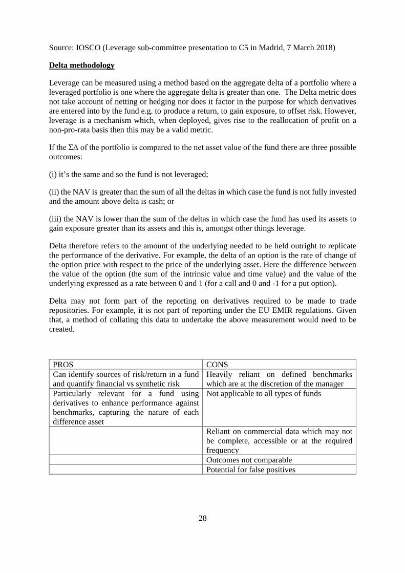
Source: IOSCO (Leverage sub-committee presentation to C5 in Madrid, 7 March 2018)

Delta methodology

Leverage can be measured using a method based on the aggregate delta of a portfolio where a leveraged portfolio is one where the aggregate delta is greater than one. The Delta metric does not take account of netting or hedging nor does it factor in the purpose for which derivatives are entered into by the fund e.g. to produce a return, to gain exposure, to offset risk. However, leverage is a mechanism which, when deployed, gives rise to the reallocation of profit on a non-pro-rata basis then this may be a valid metric.

If the ΣΔ of the portfolio is compared to the net asset value of the fund there are three possible outcomes:

(i) it’s the same and so the fund is not leveraged;

(ii) the NAV is greater than the sum of all the deltas in which case the fund is not fully invested and the amount above delta is cash; or

(iii) the NAV is lower than the sum of the deltas in which case the fund has used its assets to gain exposure greater than its assets and this is, amongst other things leverage.

Delta therefore refers to the amount of the underlying needed to be held outright to replicate the performance of the derivative. For example, the delta of an option is the rate of change of the option price with respect to the price of the underlying asset. Here the difference between the value of the option (the sum of the intrinsic value and time value) and the value of the underlying expressed as a rate between 0 and 1 (for a call and 0 and -1 for a put option).

Delta may not form part of the reporting on derivatives required to be made to trade repositories. For example, it is not part of reporting under the EU EMIR regulations. Given that, a method of collating this data to undertake the above measurement would need to be created.

PROS CONS Can identify sources of risk/return in a fund and quantify financial vs synthetic risk

Heavily reliant on defined benchmarks which are at the discretion of the manager

Particularly relevant for a fund using derivatives to enhance performance against benchmarks, capturing the nature of each difference asset

Not applicable to all types of funds

Reliant on commercial data which may not be complete, accessible or at the required frequency

Outcomes not comparable Potential for false positives

29

Appendix C – Step 2 Step 2 Applications: Example for Market risk

This section lists possible measures of market risk that authorities may find useful for their Step 2 programme. This list of indicators should not be considered to be exhaustive and some indicators might not be relevant for funds selected for further analysis. Therefore, Authorities might need to tailor their Step 2 analysis to the type of funds and to their strategy. Portfolio’s sensitivity

Information on the sensitivity of funds’ portfolio to market changes are one tool to evaluate a fund’s market risk. The below list of indicators is the most common set of portfolio sensitivities currently in use: Net DV01: the Net DV01 measures the sensitivity of a portfolio to a 1bp increase in interest rate. This information could be considered in buckets defined by maturity of the security, e.g., <5yrs, 5-15yrs and >15yrs. CS01: the CS measures the sensitivity of a portfolio due to a 1bp increase in credit spread. This information could be considered in buckets defined by maturity of the security, e.g., <5yrs, 5-15yrs and >15yrs. Net Equity Delta: the Net Equity Delta measures the sensitivity of a portfolio to movements in equity prices. Vega exposure: the Vega exposure measures the sensitivity of a portfolio to a 1bp increase in implied volatilities. Net FX Delta: the Net FX Delta measures the sensitivity of a portfolio to an increase in currency rates relative to the base currency of the fund. Net Commodity Delta: the Net Commodity Delta measures the sensitivity of a portfolio to movements in commodity prices.

Value at Risk (VaR)

The VaR is a measure of the maximum potential loss due to market risk rather than leverage. More particularly, the VaR approach measures the maximum potential loss at a given confidence level (probability) over a specific period of time under normal market conditions. For example if the VaR (1 day, 99%) of a fund equals $4 million, this means that, under normal market conditions, the funds can be 99% confident that a change in the value of its portfolio would not result in a decrease of more than $4 million in 1 day. Because VaR is a measure of potential losses, when two or more funds with similar GNE are compared, it is one data point that can help to identify which ones are more likely to pose financial systemic risk, reducing their liquidity faster or employ certain risk-taking strategies. Furthermore, VaR may be used to distinguish between funds, with similar economic exposures, employing derivatives for either adding risk or for reducing market risk.

30

Similar analysis can be carried out using other type of statistical measures such as Relative VaR for benchmarking market risk and Conditional VaR to improve tail risk analysis. These analyses are more informative if stress tested values are also taken into consideration and constantly back-tested. However, VaR needs to be carefully utilised as it is dependent strictly on trading conditions and volatility patterns of the underlying investment. A variety of models exists for estimating VaR17 and in certain jurisdictions funds have to comply with specific VaR limits with prescribed methodologies (i.e. model of VaR to be used, precise reporting period, interval of confidence, holding period etc.). However, IOSCO believes that it would not be appropriate to recommend specific parameters for the computation

17 Each model has its own set of assumptions, advantages and drawbacks. Common models include the

parametric (Variance Covariance) model, the Historical Simulation model and the Monte Carlo Simulation model. For instance, for funds investing largely in financial derivatives presenting non-linear risk features, the parametric VaR model would not appropriate and Historical Simulation model or a Monte-Carlo model might best suited.

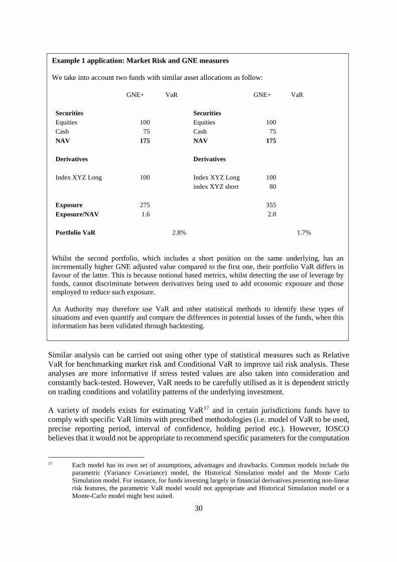
Example 1 application: Market Risk and GNE measures We take into account two funds with similar asset allocations as follow:

GNE+ VaR GNE+ VaR Securities Securities Equities 100 Equities 100 Cash 75 Cash 75 NAV 175 NAV 175 Derivatives Derivatives Index XYZ Long 100 Index XYZ Long 100 index XYZ short 80 Exposure 275 355 Exposure/NAV 1.6 2.0 Portfolio VaR 2.8% 1.7%

Whilst the second portfolio, which includes a short position on the same underlying, has an incrementally higher GNE adjusted value compared to the first one, their portfolio VaR differs in favour of the latter. This is because notional based metrics, whilst detecting the use of leverage by funds, cannot discriminate between derivatives being used to add economic exposure and those employed to reduce such exposure. An Authority may therefore use VaR and other statistical methods to identify these types of situations and even quantify and compare the differences in potential losses of the funds, when this information has been validated through backtesting.

31

of the VaR at a global level and encourages those Authorities that use or consider VaR in their step 2 analyses to consider developing local framework tailored to their market. Step 2 Applications: Example for Counterparty risk

Risk type description

A risk that is always present with leveraged funds is counterparty risk. For this reason, Authorities may be interested in estimating the losses the Fund may represent as part of their Step 2 programme. Counterparty Risk refers to the threat to each party of a contract that the other party will not live up to its contractual obligations. In the fund management context, the fund may pose counterparty risks to the other party of the contract, and, likewise, the other party may pose counterparty risk to the fund. In some cases, counterparty risk is present in only one of the parties, while in other cases the risk is present in both parties. In any scenario, the estimation by the Authority is useful for both its financial system analysis and investor protection programmes. It is often the case that counterparty risk is mitigated by the posting of collateral by one or both of the parties to a financial contract, with the amount of collateral related to the level of potential loss from the default of the counterparty. In the case of derivatives, it is more complex to measure the extent of the counterparty risk created by the derivative. If a fund wants to gain exposure to $100 of an underlying asset, it could borrow $100 and purchase the asset (resulting in counterparty risk of $100 for the lender), or it could purchase a future contract that gives exposure to $100 of that asset. The counterparty risk that is embedded in the derivatives contract is not necessarily $100: assuming the fund has taken a long position, it will only owe its counterparty an amount equal to any decline in value of the underlying reference asset, which is unlikely to be the full $100. Measuring the potential loss to a counterparty is therefore crucial in mitigating the potential consequences of a default by a counterparty.

Example 1: potential losses estimation – asset classes based

One way of approximating the results of the calculations required to compute counterparty risk is to group assets with relatively similar distributions together and assign a specific value to all assets in that group. These groups could be more or less granular and examples are provided below of current approaches used in other contexts. An Authority could, for example, differentiate between fund exposures by maturity or duration for the relevant asset classes and distinguish between investable and non-investable credit grades. The below table is an enhanced version of the example previously discussed in the Consultation paper18.

18 See table under GNE Section.

32

Cash and cash equivalents Long Short Long Short Long Short Long ShortEquity securitiesHigh-quality sovereign bondsOther fixed income securities(with maturity buckets)Non-base currency holdingsOther securitiesPhysical commoditiesEquity derivativesInterest rate derivativesCredit derivatives (Investment Grade)Credit derivatives (Non-Investment Grade)Foreign exchange derivativesCommodity derivativesOther derivativesTOTALS

* The buckets' ranges and use of maturity vs duration depend on the estimates of counterparty risks embedded in different maturity buckets adopted by the National Competent Authority

1-5 years 5> years

Exposure by Maturity or Duration*

Market Exposure

Position

Gro

ss n

otio

nal v

alue

(h

owev

er d

efin

ed)

0-1 years

Mar

ket v

alue

Investment Type

Tables of values that try to capture the counterparty risks embedded in different derivatives type and maturity buckets have been produced for use in the banking sector (BASEL III) and in margining of OTC derivatives contracts (BIS/IOSCO). The National Competent Authority may use these example tables, reproduced below, for these types of computations: BASEL III

Credit CreditInvest. Grade

non-Invest. Grade

0-1 years 0.0% 1.0% 5.0% 10.0% 6.0% 7.0% 10.0%

1-5 years 0.5% 5.0% 5.0% 10.0% 8.0% 7.0% 12.0%

> 5 years 1.5% 7.5% 5.0% 10.0% 10.0% 8.0% 15.0%

MaturityInterest Rates FX & Gold Equity

Precious Metals Others

BIS/IOSCO

0-2 years 1.0% 6.0% 2.0% 15.0% 15.0% 15.0%2-5 years 2.0% 6.0% 5.0% 15.0% 15.0% 15.0%> 5 years 4.0% 6.0% 10.0% 15.0% 15.0% 15.0%

CommoditiesInterest Rates

FX & GoldDuration Credit Equity Other

The coefficients on the tables above are multiplied by the notional amount of the derivatives contract to arrive at a counterparty risk measure. For example, let us take a 3-year interest rate future. Using the

33

coefficients in the BASEL III table, the counterparty risk of a $1m interest rate futures contract would be $5,000, while using the BIS table it would be $20,000. Unlike in the case of borrowing $1m, where the whole $1m is at risk if not repaid, in the case of a $1m position in interest rate futures, the whole $1m is not at risk. In an unfavourable environment, where the counterparty defaults and the underlying asset experiences a severely negative price change, the potential loss is going to be closer to $20,000 than $1m. The tables above could be constructed or modified by an Authority with the most conservative figures of each of the two tables above or other values as determined by the Authority, and could also be extended by introducing additional categories (single equities, equity indices, government bonds, corporate bonds, developed versus emerging markets) or maturity/duration buckets, depending on the nature and scale of the market. Although using tables such as the ones above is not as precise as modelling each individual asset would be, it has advantages as it is simple and quick to implement and it has low model risk. Furthermore, Authorities can automatically apply the calculations without requiring further information from any funds under consideration. By dividing that measure of counterparty loss by the NAV of the fund, we have a measure of how much any potential losses incurred by derivative positions can be covered by the assets in the fund. Some of those assets might be posted as either initial margins or collateral with respect to the derivatives positions; the rest are other assets that the fund owns that are unencumbered. Unencumbered assets could be cash (unencumbered cash) or other assets, with potentially various degrees of liquidity.

34

Example 2: Potential losses estimation – whole netted portfolio approach

In the case of derivatives with non-linear payoffs, such as options, the counterparty risk of one party is not the same as that of the other party, so one has to choose which side it is interested in. In the case of funds, one can calculate the counterparty risk that the fund poses to all of its counterparties, and the counterparty risk that a fund’s counterparty pose to it. In this context, an Authority may want to have a more precise estimate of the fund’s counterparty risk looking at the details of the whole portfolio. For this approach it is necessary to add all the counterparty

Example 2 application: Counterparty Risk and GNE measures Below is an example of the combination of counterparty risk (CR) analysis by asset class with GNE measure for a fund. The example ignores the correlation adjustments for simplicity.

Notional GNE GNE+ CR Asset Classes (Basel)

CR Asset Classes

(BIS/IOSCO) Securities Equities 100 100 100 100 100 Bonds 50 50 50 50 50 Cash 75 75 75 75 75 NAV 225 225 225 225

Derivatives

Equities > 5y 100 100 100 10 15 Interest Rates (3Y) 1000 1000 120 5 20 FX (<1Y) 300 300 300 3 18 IG Credit (1.5Y) 200 200 200 10 4

Exposure 1825 945 Exposure/NAV 8.1 4.2

CP Exposure 28 57 CP Exposure/NAV 12% 25%

The portfolio above has a leverage measure of 8.1 times NAV, using GNE without adjustments, and a leverage of 4.2 times NAV using Adjusted GNE. However, GNE and Adjusted GNE do not say anything about the counterparty risk of the fund. Using a CR metric with BASEL III coefficients, the counterparty risk of the fund is 12% of the NAV, while using the BIS/IOSCO coefficients the counterparty risk of the fund is 25%. Using a CR metric with BIS/IOSCO calculation, this tells us that in an extremely unfavourable scenario, the fund is likely to lose one quarter of its Net Asset Value. Presumably, in that scenario also the securities held by the fund will suffer, so a useful measure to look at is the Unencumbered Cash over NAV (see the Examples of Supplementary Data of this Appendix).

35

risk measures from all derivatives in the portfolio, with the caveat of ignoring the possibility that the derivatives positions in a portfolio might be uncorrelated, or even negatively correlated, in which case they will not all experience a 99th percentile event at the same time. In such scenario, netting and hedging of positions could be allowed in a similar way as with the NNE metric discussed for Step 1. On top of that, a correlation matrix could be used to allow for the diversification benefit of positions that are not perfectly correlated. Authorities implementing such scheme may need to estimate correlation parameters for the same asset classes used while collecting funds’ information. An example of similar computations has been produced by ISDA in the context of its Standard Initial Margin Model for non-cleared OTC derivatives. We reproduce the latest sample of correlation between risk classes within products classes below19:

A risk-based measure of leverage could be constructed relatively simply using the methodology described above, with some netting and hedging within asset classes, and correlations between asset classes, in order to arrive at a measure of potential counterparty loss for a fund. This would be a measure of the potential loss that a fund could cause to its counterparties, and also the potential loss that a fund’s counterparties pose to it (in the case of derivatives with a linear payoff). Step 2 Applications: Example Supplementary Data

Authorities can opt to use a variety of supplementary data points to improve their analysis of a fund’s leverage. The information gathered for a Step 2 programme should be additional to those adopted for Step 1 measures. Their aim is to shed light on further risk-aspects emanating from leveraged positions, which the regulator might find very valuable in its wider analysis of leverage within investment funds. The combination of these different data points with the exposure metrics data provides for valuable input for a well-rounded analysis of risks within these funds. The following list of supplementary information is a selection of various data points which IOSCO C5 members believe to be relevant and could be used to achieve a more encompassing view on leverage-related risks within investment funds. This is neither exhaustive nor prescriptive, and it requires Authorities to implement their own version.

19 See ISDA SIMM Methodology, Version 2.1 (https://www.isda.org/a/zSpEE/ISDA-SIMM-v2.1-PUBLIC.pdf)

36

Initial margin posted (absolute amounts)

Definition: Initial margin means the collateral collected by a counterparty to cover its current and potential future exposure in the interval between the last collection of margin and the liquidation of positions or hedging of market risk following a default of the other counterparty and can refer to cash and or securities posted by an investment fund to its transacting counterparty. It is intended to protect the non-defaulting counterparty of the transaction against the loss that occurs if the cost of replacing /closing out the netting set of trades exceeds the amount of variation margin held. This can happen if the mark-to-market value of the netting set to the non-defaulting counterparty has increased since the last variation margin payment was made. Purpose/ Benefit: The absolute amount of initial margin posted provides an indication of the significance of margin trading conducted by the fund. Margin trading is usually leverage driven and can thus be used to get a better understanding of the extent to which funds are potentially leveraged. Value of cash/ unencumbered cash (absolute amounts)

Definition: Unencumbered cash refers to the amount of cash and cash equivalents available for immediate use without restriction. Purpose/ Benefit: Unencumbered cash can be considered as a key metric for funds which make significant use of derivatives and possibly need to make margin payments to fund counterparties. It can be generally expected that highly leveraged funds keep sufficient unencumbered cash at least equivalent to a multiple of the initial margin posted. The analysis of the proportions of unencumbered cash to the amount of initial margin posted by the fund can provide an indication of the robustness of the fund in terms of leverage risk that is, its likely ability to meet any additional margin calls in response to changes in the value or volatility of the underlying reference asset(s).

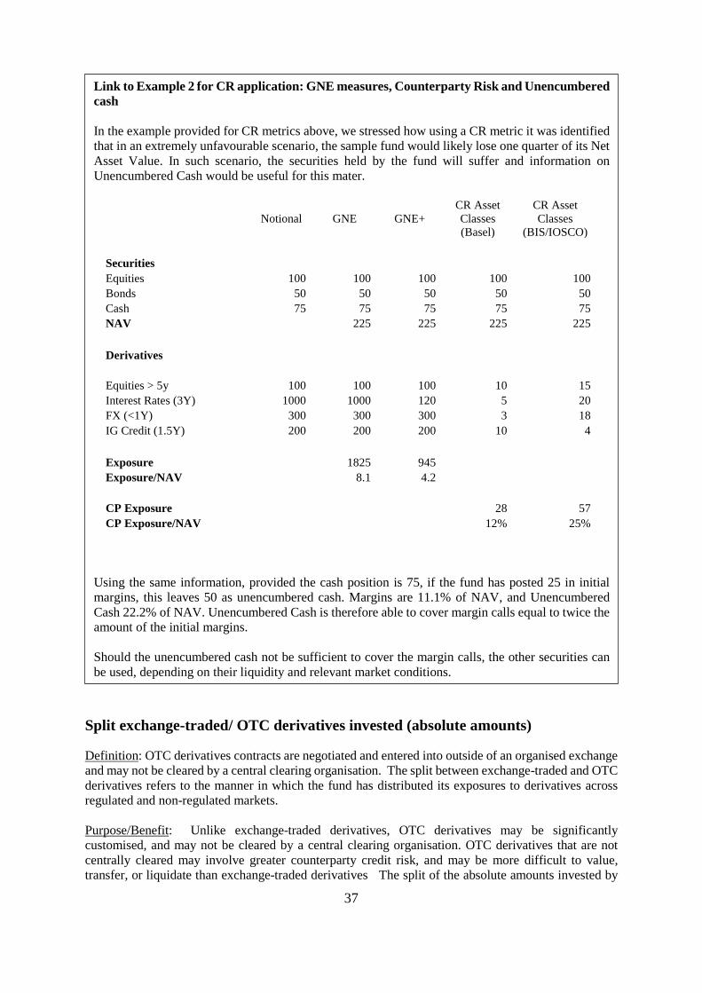
37

Split exchange-traded/ OTC derivatives invested (absolute amounts)

Definition: OTC derivatives contracts are negotiated and entered into outside of an organised exchange and may not be cleared by a central clearing organisation. The split between exchange-traded and OTC derivatives refers to the manner in which the fund has distributed its exposures to derivatives across regulated and non-regulated markets.

Purpose/Benefit: Unlike exchange-traded derivatives, OTC derivatives may be significantly customised, and may not be cleared by a central clearing organisation. OTC derivatives that are not centrally cleared may involve greater counterparty credit risk, and may be more difficult to value, transfer, or liquidate than exchange-traded derivatives The split of the absolute amounts invested by

Link to Example 2 for CR application: GNE measures, Counterparty Risk and Unencumbered cash In the example provided for CR metrics above, we stressed how using a CR metric it was identified that in an extremely unfavourable scenario, the sample fund would likely lose one quarter of its Net Asset Value. In such scenario, the securities held by the fund will suffer and information on Unencumbered Cash would be useful for this mater.

Notional GNE GNE+ CR Asset Classes (Basel)

CR Asset Classes

(BIS/IOSCO) Securities Equities 100 100 100 100 100 Bonds 50 50 50 50 50 Cash 75 75 75 75 75 NAV 225 225 225 225

Derivatives

Equities > 5y 100 100 100 10 15 Interest Rates (3Y) 1000 1000 120 5 20 FX (<1Y) 300 300 300 3 18 IG Credit (1.5Y) 200 200 200 10 4

Exposure 1825 945 Exposure/NAV 8.1 4.2

CP Exposure 28 57 CP Exposure/NAV 12% 25%

Using the same information, provided the cash position is 75, if the fund has posted 25 in initial margins, this leaves 50 as unencumbered cash. Margins are 11.1% of NAV, and Unencumbered Cash 22.2% of NAV. Unencumbered Cash is therefore able to cover margin calls equal to twice the amount of the initial margins. Should the unencumbered cash not be sufficient to cover the margin calls, the other securities can be used, depending on their liquidity and relevant market conditions.

38

the fund in the two different types of products can provide an indication of the type of market (regulated v/s unregulated) on which leverage is incurred and information about whether contracts are centrally cleared can provide information about counterparty risks. It provides further detail on the degree of riskiness and complexity of the investment strategy of the fund. Amount of cash borrowing (unsecured and secured (collateralised)) (absolute amounts)

Definition: A fund can increase its market exposure beyond its net asset value by entering into derivatives, as discussed above, or by making investments with borrowed money. Purpose/ Benefit: The ratio of borrowed cash to the gross assets or net assets, especially if reported across time (possibly also with Min./Max./Average), can provide an indication of the extent to which the fund is usually leveraged. Considering the universe of funds with a comparable gross / net assets, the higher the ratio, the more leveraged is the fund. In case of stressed markets conditions/market breakdown, the funds exhibiting higher ratios may be exposed to losses of a higher magnitude. Amount of synthetic Borrowing via derivatives (absolute amounts)

Definition: Derivatives are mainly used by funds for hedging and investment purposes. Derivatives (such as Futures, Forwards and Options) and securities can also be combined in such a way that the resulting cash flows have similarities to a cash borrowing transaction. In this case, the fund is having recourse to synthetic borrowing via derivatives.

Purpose/ Benefit: The ratio of synthetic borrowing to the Assets under management (AuM) or total net assets (TNA) especially if reported across time (possibly also with Min./Max./Average), can provide a further indication of the extent to which the fund is leveraged.

Value of aggregate amount of borrowing and cash financing available to the fund (drawn / undrawn, committed / uncommitted credit lines, term financing) (absolute amounts)

Definition: In addition to effective cash borrowing by investment funds above, a fund might also have signed agreements with banks or other financing-providers to receive financing (borrowing by the fund), e.g. in case of market stress (for liquidity management purposes). Combined with borrowed cash this provides for the maximum cash financing available to a fund. Purpose/ Benefit: This provides for the maximum borrowing available to the investment fund and thus can be used to calculate the maximum extent to which a fund could leverage its portfolio through cash borrowings.

Value of collateral posted/ received (absolute amounts)

1) Cash and cash equivalent collateral 2) Security collateral (other than cash) 3) Other collateral (letters of credit or other) 4) % of posted collateral rehypothecated by counterparties/ allowed for rehypothecation

39

Definition: Collateral is usually used to reduce counterparty risk in various financial derivative transactions. The type of collateral a fund posts or receives; the diversification of its counterparties; and whether collateral is held by a third-party custodian all may be relevant considerations in analysing counterparty risk. Purpose/ Benefit: Reported collateral amounts can be used from different perspectives: (i) The amount of collateral posted by the fund can provide an indication of the extent to which

the fund is leveraged: the higher the collateral posted, the higher is the expected engagement of the fund in collateralised financial derivative transactions. The split by collateral category provides for additional information on the inherent risks of the collateral received (possibly necessity to apply haircuts).

(ii) The rehypothecation / reuse of collateral by the investment fund is usually being perceived as amplifying leverage in a fund. The practice by banks and brokers of using, for their own purposes, assets that have been posted as collateral by their clients, e.g. investment funds, increases the risk for the investment fund in case of a bank/ broker default. The use of the same asset as underlying collateral for different transactions increases the sum of exposures in the financial system and as a result creates leverage in the intermediation chain. The analysis of this variable can thus provide useful insights in the leverage build up not only in the fund but also across several financial intermediaries. It also provides valuable information on further risks with counterparties of the investment fund. The re-hypothecation rate could be expressed as follows:

a. the ratio between the total mark-to-market value of all collateral re-hypothecated by the

counterparty and the mark-to-market value of all the collateral posted by the fund; and

b. the ratio between the total mark-to-market value of all collateral re-hypothecated by the fund and the mark-to-market value of all collateral received by the fund.